Approximately optimal domain adaptation
with Fisher’s Linear Discriminant

Abstract

We propose a class of models based on Fisher’s Linear Discriminant (FLD) for domain adaptation. The class entails a convex combination of two hypotheses: i) an average hypothesis representing previously encountered source tasks and ii) a hypothesis trained on a new target task. For a particular generative setting, we derive the expected risk of this combined hypothesis with respect to the target distribution and propose a computable approximation. This is then leveraged to estimate an optimal convex coefficient that exploits the bias-variance trade-off between source and target information to arrive at an optimal classifier for the target task. We study the effect of various generative parameter settings on the relative risks between the optimal hypothesis, hypothesis i), and hypothesis ii). Furthermore, we demonstrate the effectiveness of the proposed optimal classifier in several EEG- and ECG-based classification problems and argue that the optimal classifier can be computed without access to direct information from any of the individual source tasks, leading to the preservation of privacy. We conclude by discussing further applications, limitations, and potential future directions.

1 Introduction

In problems with limited context-specific labeled data, machine learning models often fail to generalize well. Modern machine learning approaches such as transfer learning (Pan & Yang, 2010; Weiss et al., 2016), domain adaptation (Sun et al., 2015), meta-learning (Vilalta & Drissi, 2002; Vanschoren, 2019; Finn et al., 2019; Hospedales et al., 2021), and continual learning (Van de Ven & Tolias, 2019; Hadsell et al., 2020; De Lange et al., 2021; Vogelstein et al., 2022) can mitigate this “small data effect” but still require a sufficient amount of context-specific data to train a model that can then be updated to the context of interest. These approaches are either ineffective or unavailable for problems where the input signals are highly variable across contexts or where a single model does not have access to a sufficient amount of data due to privacy or resource constraints (Mühlhoff, 2021). Note that the terms “context” and “task” can be used interchangeably here. In this paper we deal with the physiological predictive problem – a problem with both high variability across contexts (e.g., different recording sessions or different people) and privacy constraints (e.g., biometric data is often considered sensitive and identifiable and should not be shared freely across devices).

We define the physiological predictive problem as any setting that uses biometric or physiological data (e.g., EEG, ECG, breathing rate, etc.) or any derivative thereof to make predictions related to the state of a person. The predicted state could be as high level as the person’s cognitive load or affect (Friedman et al., 2019) or as low level as which hand they are trying to move (Korik et al., 2018). The machine learning models for these problems often use expert-crafted features and a relatively simple model such as a polynomial classifier or regressor (Zhang et al., 2020a).

The standard cognitive load classification baseline using EEG data, for example, is a linear model trained using the band powers of neuroscientifically relevant frequencies (e.g., the theta band from 4-7 Hz, the alpha band from 8-12 Hz, etc. (Kandel et al., 2021)) as features (Akrami et al., 2006; Akbulut et al., 2019; Guerrero et al., 2021). Recent systems for mental state classification have explored more complicated feature sets (Chen et al., 2022) to the tune of some success. Similarly, popular ECG-based predictive systems use simple statistics related to the inter-peak intervals as features for a linear classifier to predict cognitive state (McDuff et al., 2014; Lee et al., 2022). Outperforming these simple systems is more challenging for physiological prediction compared to domains such as computer vision and natural language processing because of the high variability and privacy limitations of the input data.

To be more specific, a common approach used in modern machine learning methods is to leverage data from multiple tasks to learn a representation of the data that is effective for every task (Baxter, 2000; Zhang & Yang, 2018). Once the representation is learned from the set of tasks it can then be applied to a new task and it is assumed that the representation is similarly effective for it. If the variability across the different tasks is high then data from a large set of tasks is necessary to learn a generalizable representation (Baxter, 2000). For physiological predictive systems, there is context variability caused by changes in sensor location or quality, changes in user, and changes in environmental conditions. Hence, the variability across physiological predictive contexts is high and data from a large set of contexts is necessary to learn a transferable representation. Unfortunately, collecting data from a large set of relevant physiological contexts can be prohibitively expensive.

In this paper we propose a class of models based on Fisher’s Linear Discriminant (“FLD”) (Izenman, 2013; Devroye et al., 2013) that interpolates between i) a model that is a combination of linear models trained on previous source contexts and ii) a linear model trained only on data from a new target context. We study the class of models in a particular generative setting and derive an analytical form of the risk under the 0-1 loss with respect to the target distribution. Using this analytical risk expression, we show that we can obtain an optimal combination of model i) and model ii), that improves generalization on the target context. We compare the performance of the optimal combination to the performance of model i) and model ii) across various generative parameter settings. Finally, we empirically demonstrate that by using the analytical form of the target risk we can improve upon the performance of model i) and model ii) in real-world physiological predictive settings.

2 Problem setting

The physiological classification problem is an instance of a more general statistical pattern recognition problem (Devroye et al., 2013, Chapter 1): Given training data $\{(X_{i},Y_{i})\}_{i=1}^{n}\in\left(\mathcal{X}\times\{1,\ldots,K\}\right)^{n}$ assumed to be $i.i.d.$ samples from a classification distribution $\mathcal{P}$, construct a function $h_{n}$ that takes as input an element of $\mathcal{X}$ and outputs an element of $\{1,\ldots,K\}$ such that the expected loss of $h_{n}$ with respect to $\mathcal{P}$ is small. With a sufficient amount of data, there exist classifiers $h_{n}$ that have a statistically minimal expected loss for all $\mathcal{P}$. In the physiological prediction problem, however, there is often not enough data to adequately train classifiers and we assume, instead, that there is auxillary data (or derivatives thereof) from different contexts available that can be used to improve the expected loss.

In particular, given $\{(X_{i}^{(j)},Y_{i}^{(j)})\}_{i=1}^{n}$ assumed to be $i.i.d.$ samples from the classification distribution $\mathcal{P}^{(j)}$ for $j\in\{0,\ldots,J\}$, we want to construct a function $h^{(0)}$ that minimizes the expected loss with respect to the target distribution $\mathcal{P}^{(0)}$. We refer to the other classification distributions, $\mathcal{P}^{(1)},\ldots,\mathcal{P}^{(J)}$, as source distributions. Variations of this set up are oftentimes called the transfer learning problem or domain adaptation problem and is, again, not unique to physiological prediction. Generally, for the classifier $h^{(0)}$ to improve upon the single-task classifier $h_{n}$, the source distributions need to be related to the target distribution such that the information learned when constructing the mappings from the input space to the label space in the context of the source distributions $\mathcal{P}^{(1)},\ldots,\mathcal{P}^{(J)}$ can be “transferred” or “adapted” to the context of the target distribution $\mathcal{P}^{(0)}$ (Baxter, 2000).

The physiological prediction problem imposes one additional constraint compared to the standard setup: the data from one individual must remain private to the individual (Mühlhoff, 2021). The method we propose in Section 3 addresses this constraint by leveraging the parametric model that relates the source and target classifiers.

3 A Generative Model

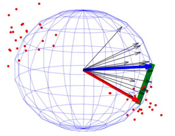
Figure 1: A geometric illustration of the generative assumptions, information constraints, and the model class under study. The red dots represent the data from the target distribution, the red arrow represents an estimate of the projection vector for the target distribution, the grey arrows represent source projection vectors, the blue arrow represents the average-source projection vector, and the green line interpolating between the blue and red arrows represents the possible end points of a convex combination of the red and blue arrows.

Our goal is to develop a private (in some sense, see Section3.5) and optimal classifier that can leverage information from data drawn from the target and source distributions. For this purpose, we first put relatively strict generative assumptions on the data and then make the relationship between the target distribution and the source distributions explicit.

In particular, we assume that $\mathcal{P}^{(j)}$ is a binary classification distribution that can be described as follows:

$$\mathcal{P}^{(j)}=\pi^{(j)}\;\mathcal{N}\left(\nu^{(j)},\Sigma^{(j)}\right)+(1-\pi^{(j)})\;\mathcal{N}\left((-1)\nu^{(j)},\Sigma^{(j)}\right);\quad\text{for }j\in\{0,\ldots,J\}.$$ (1)

That is, $\mathcal{P}^{(j)}$ is a mixture of two Gaussians such that the midpoint of the class conditional means is the origin and that the class conditional covariance structures are equivalent. Note that $\mathcal{P}^{(j)}$ is uniquely parameterized by $\nu^{(j)},\Sigma^{(j)},$ and $\pi^{(j)}$. It is known that Fisher’s Linear Discriminant function is optimal under 0-1 loss for distributions of the form described in Eq. (1) (Devroye et al., 2013, Chapter 4). Recall that Fisher’s Linear Discriminant function is the classifier defined as

$$h_{FLD}(x)=\mathbb{1}\left\{\omega^{\top}x>c\right\},$$ (2)

where $\mathbb{1}\{s\}$ is 1 if $s$ is true and $0$ otherwise and where

$$\omega=(\Sigma_{0}+\Sigma_{1})^{-1}(\nu_{1}-\nu_{0})\quad\quad\text{and}\quad\quad c=\omega^{\top}\left(\nu_{0}+\nu_{1}\right)+\log\frac{\pi_{0}}{\pi_{1}}.$$

Here $\nu_{i},\Sigma_{i}$ and $\pi_{i}$ are the mean, covariance matrix, and prior probability pertaining to class $i\in\{0,1\}$. For a distribution $\mathcal{P}$ of the form described in Eq. 1, and assuming $\pi=0.5$ for simplicity, the above expressions reduce to $\omega=\frac{1}{2}\Sigma^{-1}(\nu_{1}-\nu_{0})$ and $c=0$. From the form of Eq. (2) it is clear that the projection vector $\omega$ is a sufficient statistic for classification under 0-1 loss with respect to the distribution $\mathcal{P}$. To this end, we will assume that for the source distributions we only have access projection vectors $\omega^{(1)},\ldots,\omega^{(J)}$.

We next make a generative assumption about the source projection vectors $\omega^{(1)},\ldots,\omega^{(J)}$ to make the relationship between the distributions explicit. Recall that the von Mises-Fisher (vMF) distribution (Fisher et al., 1993), denoted by $\mathcal{V}(\mu,\kappa)$, has realizations on the $d$-sphere and is completely characterized by a mean direction vector $\mu\in\mathbb{R}^{d}$ and a concentration parameter $\kappa\in\mathbb{R}_{\geq 0}$. When the concentration parameter is close to $0$ the vMF distribution is close to a uniform distribution on the $d$-sphere. When the concentration parameter is large, the vMF distribution resembles a normal distribution with mean $\mu$ and a scaled isotropic variance proportional to the inverse of $\kappa$.

For our analysis we assume that the source vectors $\omega^{(1)},\ldots,\omega^{(J)}\stackrel{{\scriptstyle iid}}{{\sim}}\mathcal{V}(\mu,\kappa)$ for unspecified $\mu$ and $\kappa$. This assumption forces additional constraints on the relationship between $\nu^{(j)}$ and $\Sigma^{(j)}$ in the context of Eq. (1) – namely that $||(\Sigma^{(j)})^{-1}\nu^{(j)}||_{2}=\sqrt{2}$. In our simulated settings below, the generative models adhere to this constraint. In practical applications, we can use the (little) training data that we have access to force our estimates of $\nu$ and $\Sigma$ to be conformant.

3.1 A Simple Class of Classifiers

With the generative assumptions described above, we propose a class of classifiers $\mathcal{H}$ that can effectively leverage the information available with just access to the projection vectors:

$$\mathcal{H}:=\left\{h_{\alpha}(x)=\mathbb{1}\left\{\left(\underbrace{\alpha\omega^{(0)}+(1-\alpha)\sum_{j=1}^{J}\omega^{(j)}}_{\omega_{\alpha}}\right)^{\top}x>0\right\}:\alpha\in[0,1]\right\}.$$

The set $\mathcal{H}$ is exactly the classifiers parameterized by the convex combinations of the target projection vector and the sum of the source projection vectors. We refer to this convex combination as $\omega_{\alpha}$. Letting $\bar{\omega}:=\frac{1}{J}\sum_{j=1}^{J}\omega^{(j)}$, we note that $\omega_{\alpha}$ can be reparametrized in the context of the vMF distribution with the observation that

$$(1-\alpha)\sum_{j=1}^{J}\omega^{(j)} =\frac{J(1-\alpha)||\bar{\omega}||}{||\bar{\omega}||}\bar{\omega}$$

$$=J(1-\alpha)||\bar{\omega}||\;\hat{\mu},$$

where $\hat{\mu}=\bar{\omega}/||\bar{\omega}||$ is the maximum likelihood estimate for the mean direction vector of the vMF distribution. By letting $\alpha\leftarrow\frac{\alpha}{\alpha+J(1-\alpha)||\bar{\omega}||}$ we maintain the same set $\mathcal{H}$ but make the individual classifiers more amenable to analysis. Figure 1 illustrates the geometry of $\mathcal{H}$ for $d=3$.

We view different decision rules in $\mathcal{H}$ as elements along a classical bias-variance trade off curve parameterized by $\alpha$ (Belkin et al., 2019). In particular, when the amount of data available from the target distribution is small, the projection induced by an $\alpha$ value closer to 1 can be interpreted as a high variance, low bias estimate of the target projection vector. Conversely, an $\alpha$ value of 0 can be interpreted as a low variance, high bias estimate. In situations where the concentration parameter $\kappa$ is relatively large, for example, we expect to prefer combinations that favor the average-source vector. We discuss this in more detail and in the context of different parameter settings for our generative model in Section 3.4.

3.2 Approximating optimality

We define the optimal classifier $h_{\alpha^{*}}$ in the set $\mathcal{H}$ as the classifier that minimizes the expected risk with respect to the target distribution $\mathcal{P}^{(0)}$. Given the projection vectors $\{\omega^{(j)}\}_{j=1}^{J}$ and the target class conditional mean and covariance, $\nu^{(0)}$ and $\Sigma^{(0)}$, the risk (under the 0-1 loss) of a classifier $h_{\alpha}\in\mathcal{H}$ is

$$R\left(h_{\alpha}\mid\{\omega^{(j)}\}_{j=1}^{J},\nu^{(0)},\Sigma^{(0)}\right)=\Phi\left(\frac{-\omega_{\alpha}^{\top}\nu^{(0)}}{\sqrt{\omega_{\alpha}^{\top}\Sigma^{(0)}\omega_{\alpha}}}\right)$$

for $\mathcal{P}^{(0)}$ of the form described in Eq. (1) and where $\Phi$ is the cumulative distribution function of the standard normal. The derivation is given in the appendix A. In practice, the source projection vectors, source thresholds, target class conditional mean and covariance structure are all estimated. Based on the above risk, we can define the expected risk of $h_{\alpha}$ as,

$$\mathcal{E}(h_{\alpha})=\mathbb{E}_{\omega_{\alpha}}\left[R\left(h_{\alpha}\mid\{\omega^{(j)},\}_{j=1}^{J},\nu^{(0)},\Sigma^{(0)}\right)\right].$$ (3)

Unfortunately, despite the strong distributional assumptions we have in place, the expected risk is too complicated to analyze entirely. Instead, we approximate $\mathcal{E}(h_{\alpha})$ with $\hat{\mathcal{E}}(h_{\alpha})$, which we can evaluate via Monte Carlo integration by sampling from the distribution of $\omega_{\alpha}$ (derived in Section 3.3) and using the plug-in estimates for $\nu^{(0)}$ and $\Sigma^{(0)}$.

Using this risk function, we can search for optimal $\alpha^{\ast}$ that minimizes the expected risk over $\alpha\in[0,1]$. The procedure for calculating $\alpha^{\ast}$ is outlined in Algorithm 1. For the remainder of this section, we use $\hat{t}$ to denote an estimate of the parameter $t$.

Algorithm 1 Calculating the optimal convex coefficient

1:target task class conditional mean $\hat{\nu}_{0}^{(0)}$ and $\hat{\nu}_{1}^{(0)}$, target task class conditional covariance $\hat{\Sigma}^{(0)}$, normalized source proj. vectors $\{\hat{\omega}^{(j)}\}_{j=1}^{J}$, the number of bootstrap samples $B$.

2:$\hat{\omega}^{(0)}\leftarrow\textsc{Normalize}\left(\frac{1}{2}(\hat{\Sigma}^{(0)})^{-1}(\hat{\nu}_{1}^{(0)}-\hat{\nu}_{0}^{(0)})\right)$ $\triangleright$ Estimate the target proj. vector

3:$\hat{\mu}\leftarrow$ Normalize$\left(\frac{1}{J}\sum_{j=1}^{J}\hat{\omega}^{(j)}\right)$ $\triangleright$ Estimate vMF mean direction vector

4:$\hat{\Psi}\leftarrow$ Variance$\left(\hat{\mu}\right)$ $\triangleright$ Variance of vMF mean direction vector

5:$\hat{\Sigma}_{\omega}\leftarrow$ Variance$\left(\hat{\omega}^{(0)}\right)$ $\triangleright$ Variance of the target proj. vector (see section 3.3)

6:for each $\alpha\in[0,1]$ do

7:     $\hat{\omega}_{\alpha}\leftarrow\left(\alpha\;\hat{\omega}^{(0)}+(1-\alpha)\;\hat{\mu}\right)$ $\triangleright$ Average convex combination

8:     $\hat{\Sigma}_{\alpha}\leftarrow\alpha^{2}\hat{\Sigma}_{\omega}+(1-\alpha)^{2}\hat{\Psi}$ $\triangleright$ Variance of average convex combination

9:     for each $b$ in $\{1,..,B\}$ do

10:         $\omega_{b}\leftarrow\mathcal{N}\left(\hat{\omega}_{\alpha},\hat{\Sigma}_{\alpha}\right)$ $\triangleright$ Sample from appropriate normal distribution

11:         $r_{b}\leftarrow\Phi\left(-\frac{\omega_{b}^{\top}\hat{\nu}^{(0)}}{\sqrt{\omega_{b}^{\top}\hat{\Sigma}^{(0)}\;\omega_{b}}}\right)$ $\triangleright$ Calculate error for sample

12:     end for

13:     $\hat{\mathcal{E}}\left({\alpha}\right)\leftarrow\frac{1}{B}\sum_{b=1}^{B}r_{b}$ $\triangleright$ Calculate risk

14:end for

15:$\alpha^{\ast}\leftarrow\operatornamewithlimits{argmin}_{\alpha}\hat{\mathcal{E}}(\alpha)$ $\triangleright$ Select optimal alpha

3.3 Deriving the asymptotic distribution of $\hat{\omega}_{\alpha}$

We are interested in deriving a data-driven method for finding the element of $\mathcal{H}$ that performs best on the target task. For this, we rely on the asymptotic distribution of $\hat{\omega}_{\alpha}=\alpha\hat{\omega}^{(0)}+(1-\alpha)\hat{\mu}$. First, we consider the estimated target projection vector $\hat{\omega}^{(0)}=\frac{1}{2}(\hat{\Sigma}^{(0)})^{-1}(\hat{\nu}_{1}^{(0)}-\hat{\nu}_{0}^{(0)})$ as a product of the independent random variables, $A:=n(\hat{\Sigma}^{(0)})^{-1}$ and $\tau:=\frac{1}{2}(\hat{\nu}_{1}^{(0)}-\hat{\nu}_{0}^{(0)})$ and note that $A\sim W_{d}(n,\Sigma^{(0)})$ is distributed according to a Wishart distribution with $n$ degrees of freedom and scatter matrix $\Sigma^{(0)}$ and that $\tau\sim\mathcal{N}_{d}(\nu^{(0)},\Sigma^{(0)}/n)$ is normally distributed. For large $n$, the random vector $nA^{-1}\tau$ has the asymptotic distribution given by,

$$\sqrt{n}\left(nA^{-1}\tau-(\Sigma^{(0)})^{-1}\nu\right)\stackrel{{\scriptstyle d}}{{\longrightarrow}}\mathcal{N}_{d}(0,\tilde{\Sigma}),$$

where $\tilde{\Sigma}=(1+(\nu^{(0)})^{\top}(\Sigma^{(0)})^{-1}\nu^{(0)})(\Sigma^{(0)})^{-1}-(\Sigma^{(0)})^{-1}\nu^{(0)}(\nu^{(0)})^{\top}(\Sigma^{(0)})^{-1}$ (Kotsiuba & Mazur, 2016). It follows that $\hat{\omega}^{(0)}$ is aymptotically distributed according to a normal distribution with mean $\omega^{(0)}=(\Sigma^{(0)})^{-1}\nu^{(0)}$ and covariance matrix $\Sigma_{\omega}:=\tilde{\Sigma}/n$.

Next, we observe that $\hat{\mu}$ is the sample mean direction computed from $J$ i.i.d samples drawn from a $\mathcal{V}(\mu,\kappa)$. For large $J$ we have $\hat{\mu}$ asymptotically distributed as a normal distribution with mean $\mu$ and covariance $\Psi$ given by

$$\Psi=\left(\frac{1-\frac{1}{J}\sum_{j=1}^{J}(\mu^{\top}\omega^{(j)})^{2}}{J\|\bar{\omega}\|}\right)^{1/2}I_{d},$$

where $I_{d}$ is the $d\times d$ identity matrix (Fisher et al., 1993).

Finally, since $\hat{\omega}$ and $\hat{\mu}$ are independent and asymptotically normally distributed, for large $n$ and $J$, we have that

$$\hat{\omega}_{\alpha}\sim\mathcal{N}\left(\underbrace{\alpha\omega^{(0)}+(1-\alpha)\mu}_{\omega_{\alpha}},\underbrace{\alpha^{2}\Sigma_{\omega}+(1-\alpha)^{2}\Psi}_{\Sigma_{\alpha}}\right).$$ (4)

We use samples from this asymptotic distribution when evaluating the risk function described in Eq. (3).

3.4 Simulations

In this section we study the difference between the true-but-analytically-intractable risk and our proposed approximation under a fixed set of generative model parameters as well as the effect of different generative model parameters on the relative risks of the target classifier, the average-source classifier, and the optimal classifier derived in Section 3.2. For each simulation setting we report the expected accuracy (i.e., 1 minus the expected risk) and the optimal convex coefficient $\alpha^{*}$.

Let $d$ be the dimensionality of the data. Without loss of generality, we consider a von Mises-Fisher distribution with mean direction $\mu=[1,0_{d-1}]^{\top}$ and concentration parameter $\kappa$. In all of our experiments, we fix the mixing coefficient $\pi^{(j)}=0.5$ and the class-conditional covariance $\Sigma^{(j)}=I_{d}$ for all task distributions. We sample $\nu^{(0)}$ and $\{\omega^{(j)}\}_{j=1}^{J}$ from the described vMF distribution and let $n$ be the number of samples from the target distribution. Finally, for each simulation setting we report the mean metric over 1,000 iterations and, hence, the standard error of each estimate is effectively zero.

3.4.1 Analytical versus empirical risks

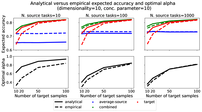
Figure 2: Comparing the analytical and empirical accuracies and optimal convex coefficient $\alpha^{\ast}$ for different amounts of target training data and number of source tasks.

Under the assumptions above, Figure 2 compares the analytical risk derived in Section 3.2 to the oracle empirical risk in the described generative setting. In particular, we simulate the generative setting by sampling 1,000 different $(\nu^{(0)},\{\omega^{(j)}\}_{j=1}^{J})$ pairs with $d=10,\kappa=10$ and varying amounts of source tasks $J$. We assume that the target class covariance and class 1 mean are known. For a given pair we sample $n\in\{10,20,50,100\}$ data from the target distribution and calculate the risk according to Eq. (3) for $\alpha\in\{0,0.1,0.2,\ldots,1.0\}$ using 100 samples from $\mathcal{N}\left(\mu_{\omega_{\alpha}},\Sigma_{\omega_{\alpha}}\right)$. The top row of Figure 2 shows these risks for $\alpha=0$ (average-source), $\alpha=1$ (target), and $\alpha=\alpha^{*}$ (optimal). The top row also includes the empirical risk where we sample 10,000 $(X,Y)$ pairs from the target distribution and evaluate the three decision functions directly. Here, the optimal vector is the convex combination of the average-source and target vectors that performs best on the test set.

Focusing on a single figure in the top row of Figure 2 we see that the gap between the analytical and empirical risks associated with the target classifier decreases as the number of samples from the target distribution increases. In the early parts of the regime the asymptotic approximation of the variance associated with the target data is not as well suited to estimate the risk as it is in the later parts of the regime. In any case, the optimal classifier is able to outperform the target classifier throughout and the analytical and empirical risks are indistinguishable for large $n$.

Now looking from the left to the right of Figure 2, we see that the gap between the analytical and empirical risks associated with the average-source and optimal classifiers decreases as we increase the number of source tasks. This is because modeling the distribution of the average-source vector as a normal distribution becoming more appropriate as the number of the source tasks increases. When simulating this setting for $J=1,000$, for example, the difference between the empirical and analytical risks associated with the average-source task is negligible.

The validity of our approximation as $n$ gets large and $J$ gets large is apparent when evaluating the differences between the optimal convex coefficients – for $J=10$ the coefficients are separated for the entire regime, for $J=100$ there is meaningful separating for small $n$ that goes away for larger $n$, and for $J=1,000$ the separation quickly becomes small. We take this as evidence that our analytical approximation is appropriate.

3.4.2 The effect of plug-in estimates, concentration, and dimensionality

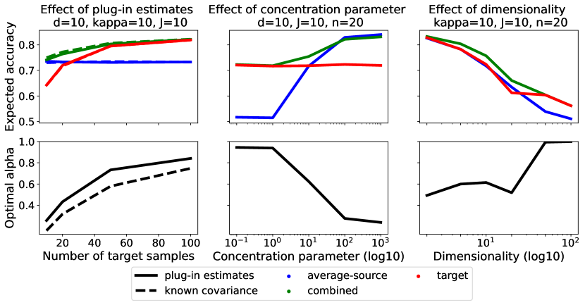
Figure 3: Studying the effect of using plug-in estimates (left) and the effect of varying different generative model parameters (center, right) on the expected accuracy of the average-source, target, and optimal classifiers and on the optimal convex coefficient.

Figure 3 shows the effect of estimating the covariance structure (left column), the effect of different vMF concentration parameters (middle column), and the effect of dimensionality (right column) on the relative accuracies of the average-source, target, and optimal classifiers and the calculated optimal convex coefficients. We fix the dimensionality to be $10$, the number of source tasks to be $100$, the vMF concentration parameter to be $10$ and the number of target samples available to be $20$ when appropriate. The classifiers are evaluated using 10,000 samples from the target distribution.

The left column of Figure 3 illustrates the effect of estimating the target task’s class conditional covariance structure $\Sigma^{(0)}$ and class 1 conditional mean $\nu^{(0)}$ and using these estimates as plug-ins for their population values when approximating the risk described in Eq. 3. In particular, we compare the expected accuracy and optimal coefficient when using the plug-in estimates (solid lines) $\hat{\Sigma}^{(0)}$ and $\hat{\nu}^{(0)}$ to using the population covariance $\Sigma^{(0)}$ and ${\nu}^{(0)}$ (dashed lines). We note that the difference between the performance of the optimal classifiers in the two paradigms is smaller than the difference between the performance of optimal classifier and the target classifier for small $n$. This behavior is expected, as the optimal classifier has access to more information through the average-source projection vector. Finally, we note that the difference between the two optimal coefficients is smaller for the poles of the regime and larger in the middle. We think that this is due to higher entropy states between wanting to use the “high bias, low variance” average-source classifier and the “low bias, high variance” target classifier.

For both the middle and right columns of Figure 3 we study only the plug-in classifiers. The middle column of Figure 3 investigates the effect of the vMF concentration parameter $\kappa$. Recall that as $\kappa$ gets larger the expected cosine distance between samples from the vMF distribution gets smaller. This means that the expected cosine distance between the average-source projection vector and the true-but-unknown target projection gets smaller. Indeed, through the expected accuracies of the average-source and target classifiers we see that the average-source classifier dominates the target classifier in the latter part of the studied regime due to the average-source vector providing good bias. Notably, the combined classifier is always as effective and sometimes better than the target classifier but is slightly less effective than the average-source classifier when $\kappa$ is large. This, again, is due to the appropriateness of modeling the average-source vector as Gaussian. The optimal convex coefficient is close to 1 when the vMF distribution is close to the uniform distribution on the unit sphere ($\kappa$ small) and closer to 0 when vMF distribution is closer to a point mass ($\kappa$ large).

The right column of Figure 3 shows the effect of the dimensionality of the classification problem on the expected accuracies and optimal coefficient. The top figure demonstrates that the optimal classifier is always as good as and sometimes better than both the average-source and target classifiers, with the margin being small when the dimensionality is both small and large. The reason the margin between the accuracies starts small, gets larger, and then becomes small again is likely due to the interplay between the estimation error associated with covariance structure and the relative concentration of the source vectors. We do not investigate this complicated interplay further. The optimal coefficient gets progressively larger as the dimensionality increases with the exception of a dip at $d=20$. We think this dip is due to a regime change in the interplay mentioned previously.

3.5 Privacy considerations

As presented in Algorithm 1 the process for calculating the optimal convex coefficient $\alpha^{*}$ requires access to the normalized source projection vectors $\{\omega^{(j)}\}_{j=1}^{J}$. This requirement can be prohibitive in applications where the data (or derivatives thereof) from a source task are required to stay local to a single device or are otherwise unable to be shared. For example, it is common for researchers to collect data in a lab setting, deploy a similar data collection protocol in a more realistic setting, and to use the in-lab data as a source task and the real-world data as a target task. Depending on the privacy agreements between the researchers and the subjects, it may be impossible to use the source data directly.

The requirements for Algorithm 1 can be changed to address these privacy concerns by calculating the average source vector $\hat{\mu}$ and its corresponding standard error $\Psi$ in the lab setting and only sharing these two parameters. Indeed, given $\hat{\mu}$ and $\Psi$ the algorithm is independent of the normalized source vectors and can be the only thing stored and shared with devices and systems collecting data from the target task.

4 Applications to physiological prediction problems

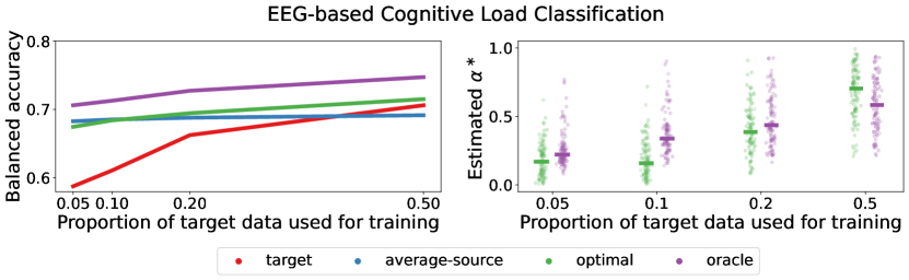
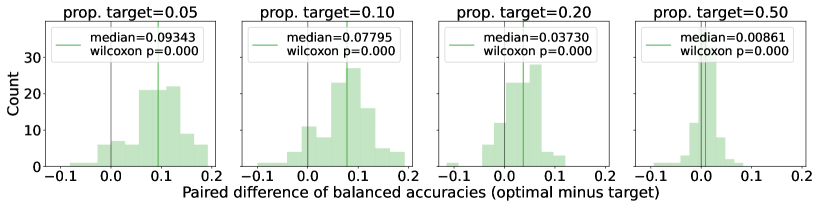
Figure 4: Balanced accuracy and relevant convex coefficients (top) and relative performance of the optimal and target classifiers (bottom) for the MATB-II cognitive load classification task.

We next study the proposed class of classifiers in the context of three physiological prediction problems: EEG-based cognitive load classification, EEG-based stress classification, and ECG-based social stress classification. In each setting we have access to data from a target study participant and the projection vectors from other participants. The data for each subject is processed such that the assumptions of Eq. (1) are matched as closely as possible. For example, we use the available training data from the target participant to force the class conditional class means to be on the unit sphere and for their midpoint to cross through the origin. Further, we normalize the learned projection vectors so that the assumption that the vectors come from a von-Mises Fisher distribution is sensible.

The descriptions of the cognitive load and stress datasets are altered versions of the descriptions found in Chen et al. (Chen et al., 2022). Unless otherwise stated, the balanced accuracy and the convex coefficient corresponding to each method are calculated using 100 different train-test splits for each participant. Conditioned on the class-type, the windowed data used for training are consecutive windows. A grid search in $\{0,0.1,0.2,\ldots,1.0\}$ was used when calculating convex coefficients.

4.1 Cognitive load (EEG)

The first dataset we consider was collected under NASA’s Multi-Attribute Task Battery II (MATB-II) protocol. MATB-II is used to understand a pilot’s ability to perform under various cognitive load requirements (Santiago-Espada et al., 2011) by attempting to induce four different levels of cognitive load – no (passive), low, medium, and high —that are a function of how many tasks the participant must actively tend to.

The data includes 50 healthy subjects with normal or corrected-to-normal vision. There were 29 female and 21 male participants and each participant was between the ages of 18 and 39 (mean 25.9, std 5.4 years). Each participant was familiarized with MATB-II and then participated in two sessions containing three segments. The three segments were further divided into blocks with the four different levels of cognitive requirements. The sessions lasted around 50 minutes and were separated by a 10 minute break. We focus our analysis on a per-subject basis, meaning there will be two sessions per subject for a total of 100 different sessions.

The EEG data was recorded using a 24-channel Smarting MOBI device and was processed using high pass (0.5 Hz) and low pass (30 Hz) filters and segmented in ten second, non-overlapping windows. Once the EEG-data was windowed we calculated the mass in the frequency domain for the theta (4-8 Hz), alpha (8-12 Hz), and lower beta (12-20 Hz) bands. We then normalized the mass of each band on a per channel basis. In our analysis we consider only the frontal channels {Fp1, Fp2, F3 F4, F7, F8, Fz, aFz}. Our choice in channels and bands is an attempt to mitigate the number of features while maintaining the presence of known cognitive load indicators (Owen et al., 2005). The results reported in Figure 4 are for this $(3\times 8)=24$-dimensional two class problem {no & low cognitive load, medium & high cognitive load}.

For a fixed session we randomly sample a continuous proportion of the participant’s windowed data $p\in\{0.05,0.1,0.2,0.5\}$ and also have access to the projection vectors corresponding to all sessions except for the target participant’s other session (i.e., we have 100 - 1 - 1 = 98 source projection vectors). As mentioned above, we use the training data to learn a translation and scaling to best match the model assumptions of Section 3.

The top left figure of Figure 4 shows the mean balanced accuracy on the non-sampled windows of four different classifiers: the average-source classifier, the target classifier, the optimal classifier, and the oracle classifier. The average-source, target, and optimal classifiers are as described in Section 3.4. The oracle classifier is the convex combination of the average-source and target projection vectors that performs the best on the held out test set. The median balanced accuracy of each classifier is the median (across sessions) calculated from the mean balanced accuracy of 100 different train-test samplings for each session.

The relative behaviors of the average-source, target and optimal classifiers in this experiment are similar to what we observe when varying the amount of target data in the simulations for large $\kappa$ – the average-source classifier outperforms the target classifier in small data regimes, the target classifier outperforms the average-source classifier in large data regimes, and the optimal classifier is able to outperform or match the performance of both classifiers throughout the regime. Indeed, in this experiment the empirical value of $\kappa$ when estimating the projection vectors using all of each session’s data is approximately 17.2.

The top right figure of Figure 4 shows scatter plots of the convex coefficients for the optimal and oracle methods. Each dot represents the average of 100 coefficients for a particular session for a given proportion of training data from the target task (i.e., one dot per session). The median coefficient is represented by a short line segment. The median coefficient for both the oracle and the optimal classifiers get closer to 1 as more target data is available. This behavior is intuitive, as we’d expect the optimal algorithm to favor the in-distribution data when the estimated variance of the target classifier is “small”.

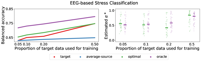
Figure 5: Balanced accuracy and relevant convex coefficients (top) and relative performance of the optimal and target classifiers on a per-participant basis (bottom) for the Mental Math EEG-based stress classification task.

The bottom row of Figure 4 is the set of histograms of the difference between the optimal classifier’s balanced accuracy and the target classifier’s balanced accuracy where each count represents a single session. These histograms give us a better sense of the relative performance of the two classifiers – a distribution centered around 0 would mean that we have no reason to prefer the optimal classifier over the target classifier and where a distribution shifted to the right of 0 would mean that we would prefer the optimal classifier to the target classifier.

For $p=0.05$ the optimal classifier outperforms the target classifier for 92 of the 100 sessions with differences as large as 19.2% and a median absolute accuracy improvement of about 9.3%. The story is similarly dramatic for $p=0.10$ with the optimal classifier outperforming the target classifier for 92 of the 100 sessions, a maximum difference of about 19.2%, and a median difference of 7.8%. For $p=0.2$ the distribution of the differences is still shifted to the right of $0$ with a non-trivial median absolute improvement of about 3.7%, a maixmum improvement of 12%, and an improvement for 81 of the sessions.. For $p=0.5$ the optimal classifier outperforms the target classifier for 76 of the 100 sessions, though the distribution is only slightly shifted to the right of $0$. The p-values, up to 3 decimal places, from the one-sided Wilcoxon’s rank-sum test for the hypothesis that the distribution of the paired differences is symmetric and centered around 0 are $0.000,0.000,0.000$, and, $0.000$ for available proportions of target data $0.05,0.1,0.2$ and $0.5$, respectively.

4.2 Stress from mental math (EEG)

In the next study we consider there are two recordings for each session – one corresponding to a resting state and one corresponding to a stressed state. For the resting state, participants counted mentally (i.e., without speaking or moving their fingers) with their eyes closed for three minutes. For the stressful state, participants were given a four digit number (e.g., 1253) and a two digit number (e.g., 43) and asked to recursively subtract the two digit number from the four digit number for 4 minutes. This type of mental arithmetic is known to induce stress (Noto et al., 2005).

There were initially 66 participants (47 women and 19 men) of matched age in the study. 30 of the participants were excluded from the released data due to poor EEG quality. Thus we consider the provided set of 36 participants first analyzed by the study’s authors (Zyma et al., 2019). The released EEG data was preprocessed via a high-pass filter and a power line notch filter (50 Hz). Artifacts such as eye movements and muscle tension were removed via ICA. We windowed the data into two and a half second chunks with no overlap and consider the two-class classification task {stressed, not stressed} with access only to the channels along the centerline {Fz, Cz, Pz} and the theta, alpha and lower beta bands described above. The results of this experiment are displayed in Figure 5 and are structured in the same way as the cognitive load results.

For this study we see relative parity between the target and average-source classifiers when $p=0.05$. In this case, the optimal classifier is able to leverage the discriminative information in both sets of information and improve the balanced accuracy. This win is maintained until the target classifier performance matches the optimal classifier performance for $p=0.5$. The poor performance of the average-source classifier is likely due to the empirical value for $\kappa$ being less than 3.

Interestingly, we do not see as clear of a trend for the median convex coefficients in the top right figure. They are relatively stagnant between $p=0.05,0.1$ and $0.2$ before jumping considerably closer to $1$ for $p=0.5$.

When comparing the optimal classifier to the target classifier on a per-participant basis directly (bottom row) it is clear that the optimal classifier is favorable: for $p=0.05,0.10$ and $p=0.2$ the optimal classifier outperforms the target classifier for 25, 24, and 24 of the 36 participants, respectively, and the median absolute difference of these wins is in the 1.8% - 2.6% range for all three settings with maximum improvements of 19.2 for $p=0.05$ , 19.2 for $p=0.1$, 12.1 for $p=0.2$. As with the cognitive load task, this narrative shifts for $p=0.5$ as the distribution of the differences is approximately centered around 0. The p-values from the one-sided rank-sum test reflect these observations: 0.001, 0.01, 0.007, and 0.896 for $p=0.05,0.1,0.2$, and $0.5$, respectively.

4.3 Stress in social settings (ECG)

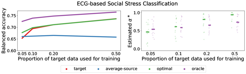
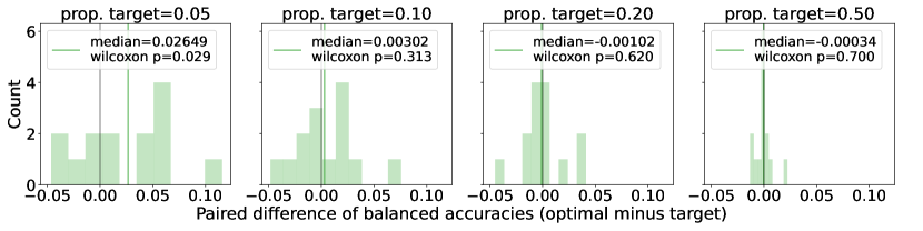
Figure 6: Balanced accuracy and relevant convex coefficients (top) and relative performance of the optimal and target classifiers on a per-participant basis (bottom) for the Social Stress, ECG-based classification task.

The last dataset we consider is the WEarable Stress and Affect Detection (WESAD) dataset. For WESAD, the researchers collected multi-modal data while participants underwent a neutral baseline condition, an amusement condition and a stress condition. The participants meditated between conditions. For our purposes, we will only consider the baseline condition where participants passively read a neutral magazine for approximately 20 minutes and the stress condition where participants went through a combination of the Trier Social Stress Test and a mental arithmetic task for a total of 10 minutes.

For our analysis, we consider 14 of the 15 participants and only work with their corresponding ECG data recorded at 700 Hz. Before featurizing the data, we first downsampled to 100 Hz and split the time series into 15 second, non-overlapping windows. We used Hamilton’s peak detection algorithm (Hamilton & Tompkins, 1986) to find the time between heartbeats for a given window. We then calculated the proportion of intervals larger than 20 milliseconds, the normalized standard deviation of the interval length, and the ratio of the high (between 15 and 40 hz) and low (between 4 and 15 hz) frequencies of the interval waveform after applying a Lomb-Scargle correction for waves with uneven sampling. These three features are known to have discriminative power in the context of stress prediction (Kim et al., 2018), though typically for larger time windows.

We report the same metrics for this dataset in Figure 6 as we do for the two EEG studies above: the mean balanced accuracies are given in the top left figure, the convex coefficients for the optimal and oracle classifiers are given in the top right and the paired difference histograms between the optimal classifier’s balanced accuracy and the target classifier’s balanced accuracy are given in the bottom row.

The relative behaviors of the classifiers in this study is similar to the behaviors in EEG-based stress study above. The optimal classifier is able to outperform the other two classifiers for $p=0.05$ and is matched by the target classifier for the rest of the regime. The average-source classifier is never preferred and the empirical value of $\kappa$ is approximately 1.5. The distributions of the optimal coefficients get closer to 1 as $p$ increases but are considerably higher compared to the MATB study for each value of $p$ – likely due to the large difference between the empirical values of $\kappa$ across the two problems.

Lastly, the paired difference histograms for $p=0.05$ favors the optimal classifier. The histograms for $p=0.1,0.2,$ and $0.5$ are inconclusive. The p-values for Wilcoxon’s rank-sum test are $0.029,0.313,0.620$ and $0.700$ for $p=0.05,0.1,0.2$ and $0.5$, respectively.

4.4 Visualizing the projection vectors

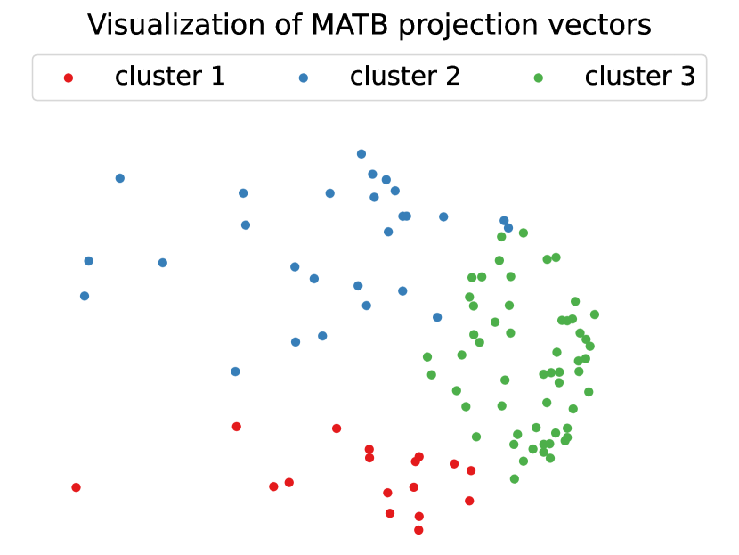
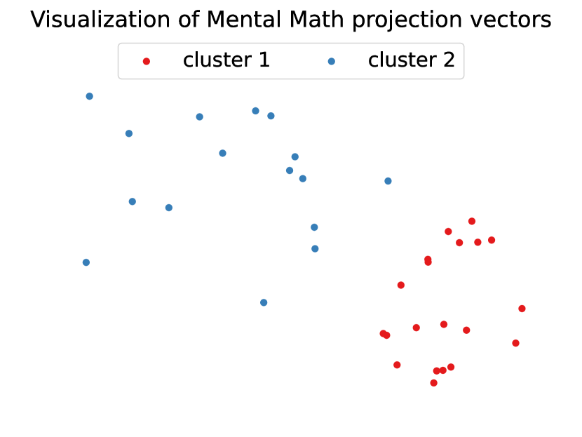
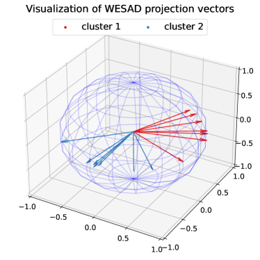
Figure 7: Visualizations of the projection vectors for each of the three datasets under study where each dot or arrow corresponds to a session. The projection vectors were estimated using the entire data from each session. For the MATB (top left) and Mental Math (top right) visualizations we show the first two principal components scaled by their corresponding eigenvalues of the $J\times J$ cosine similarity matrix. The WESAD visualization (bottom) shows the three dimensional projection vectors. Colors denote the component of a Gaussian mixture model fitted to the projection vectors.

The classification results above provide evidence that our proposed approximation to the optimal combination of the average-source and target projection vectors is useful from the perspective of improving the balanced accuracy. There is, however, a consistent gap that remains between the performance of the optimal classifier and the performance of the oracle classifier. To begin to diagnose potential issues with our model, we visualize the projection vectors from each of the tasks.

The three subfigures of Figure 7 show representations of the projection vectors for each task. The dots in the top row correspond to projection vectors from sessions from the MATB dataset (left) and the Mental Math dataset (right). The arrows with endpoints on the sphere in the bottom row correspond to projection vectors from sessions from WESAD. For these visualizations the entire dataset was used to estimate the projection vectors. The two-dimensional representations for MATB and Mental Math are first two components of the spectral embedding (Sussman et al., 2012) of the affinity matrix $A$ with entries $a_{ij}=(\omega^{(i)\top}\omega^{(j)}+1)/2$ and $a_{ii}=0$. The projection vectors for the WESAD task are three dimensional and are thus amenable to visualization.

For each task we clustered the representations of the projection vectors using a Gaussian mixture model where the number of components was automatically selected via minimization of the Bayesian Information Criterion (BIC). The colors of the dots and arrows reflect this cluster membership. The BIC objective function prefers a model with at least two components to a model with a single component for all of the classification problems – meaning that modeling the distribution of the source vectors as a unimodal von-Mises Fisher distribution is likely wrong and that a multi-modal von-Mises Fisher distribution may be more appropriate. We do not pursue this idea further but do think that it is could be a fruitful future research direction if trying to mitigate the gap between the performances of the optimal and oracle classifiers.

4.5 The effect of the number of samples used to calculate $\alpha^{*}$

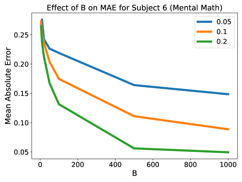
Figure 8: The effect of the number samples sampled from the distribution of $\omega_{\alpha}$ on the absolute error between the optimal $\alpha$ calculated using $B$ samples and the optimal $\alpha$ calculated using $B^{*}=10,000$ samples for subject 6 of the Mental Math dataset.

In the simulation experiments described in Section 3.4 and the applications to different physiological prediction problems in Sections 4.1, 4.2, and 4.3 we used 100 samples from the distribution of $\omega_{\alpha}$ to estimate the risk for a given $\alpha$. There is no way to know a priori how many samples is sufficient for estimating the optimal coefficient. We can, however, study how different amounts of samples effect the absolute error of the optimal coefficient compared to an coefficient calculated using an unrealistic amount of samples. For this analysis we focus on a single session from the Mental Math dataset described in 4.2. The dataset choice was a bit arbitrary. The session was chosen because it is the session where the optimal classifier performs closest to the median balanced accuracy for $p=0.1$.

Figure 8 shows the effect of $B$, the number of samples from the distribution of $\omega_{\alpha}$ used to calculate the risk for a given $\alpha$, on the mean absolute error when compared to a convex coefficient calculated using $B^{*}=10,000$ samples. The mean absolute errors shown are calculated for $p\in\{0.05,0.1,0.2\}$ by first sampling a proportion of data $p$ from the target task, training the target classifier using the sampled data, and then estimating the optimal coefficient using $B^{*}=10,000$ samples from the distribution of $\omega_{\alpha}$. We then compare this optimal coefficient to coefficient found using $B\in\{5,10,20,50,100,200,500,1000\}$ samples from the distribution of $\omega_{\alpha}$ 30 different times, calculate the absolute difference, and record the mean. The lines shown in Figure 8 is the average of 100 different training sets. In this experiment the coefficients $\alpha\in\{0,0.1,\ldots,1.0\}$ were evaluated.

There are a few things of note. First, when there is more target data available the fewer samples from the distribution of $\omega_{\alpha}$ are needed to obtain a specific value of mean absolute error. Second, the mean absolute error curves appear to be a negative exponential function of $B$ and, for this subject, it seems that the benefit of more samples decays quite quickly after $B=500$. Lastly, though the closer the convex coefficients are to the coefficient calculated using $B^{*}$ samples the more closely the classifier will perform to the analytically derived optimal classifier, the gap between the performance of the oracle classifier and the optimal classifier in the real data sections above indicates that there may be some benefit from a non-zero mean absolute error.

5 Discussion

The approximation to the optimal convex combination of the target and average-source projection vector proposed in Section 3 is effective in improving the classification performance in simulation and, more importantly, across different physiological prediction settings. The improvement is both operationally significant and statistically significant in settings where very little training data from the target distribution is available. In most Human-Computer Interface (HCI) systems an improvement in this part of the regime is the most critical as manufacturers want to mitigate the amount of configuration time (i.e., the time spent collecting labeled data) the users endure and, more generally, make the systems easier to use. We think that our proposed method, along with its privacy-preserving properties inherent to parameter estimation, is helpful towards that goal.

With that said, there are limitations in our work. For example, the derivation of the optimal convex coefficient and, subsequently, our proposed approximation is only valid for the two class problem. We do not think that an extension to the multi-class problem is trivial, though treating a multi-class problem as multiple instances of the two class problem is a potential way forward (Wu et al., 2004; Li et al., 2006).

Similarly, our choice to use a single coefficient on the average-source projection vector, as opposed to one coefficient per source task, may be limiting in situations where the source vectors are not well concentrated. In the WESAD analysis where $\kappa\approx 1.5$, for example, it may be possible to maintain an advantage over the target classifier for a larger section of the regime with a more flexible class of hypotheses. The flexibility, however, comes at the cost of privacy and computational resources. A potential middle ground between maximal flexibility and the combination of privacy preservation and computational costs modeling the distribution of the source projection vectors as a multi-modal vMF where the algorithm would only need access to the mean direction vector and standard errors associated with each constituent distribution. The visualizations in Section 4.4 provide evidence that this model may be more appropriate than the one studied here.

6 Related Works

Connection to domain adaptation theory

The problem we address in this work can be framed as a domain adaptation problem with multiple sources. While a rich body of literature (Ben-David et al., 2010; Mansour et al., 2008; Duan et al., 2012; 2009; Sun et al., 2015; Guo et al., 2018; Zhang et al., 2015; Zhao et al., 2018) have studied and discussed this setting, our work shares the most resemblance with the theoretical analysis proposed by (Mansour et al., 2008). There, the approach is to optimally combine the source hypotheses to derive a hypothesis that achieves a small error with respect to the target task which is assumed to have a distribution equal to a mixture of the source distributions. On the contrary, our work proposes a way in which we can optimally combine the average source hypothesis with the target hypothesis to achieve a minimal generalization error on the target task. Owing to the simple nature of the linear hypothesis class and task distributions under consideration, we are able to employ an analytically derived expected risk expression to find the optimal combination. This is in contrast with the studies on more general classes of hypotheses and distributions, led by the aforementioned body of literature. Moreover, De Silva et al. (2022) reveals that the target generalization error can be a non-monotonic function of the number of source samples and points out that an optimally weighted empirical risk minimization between target and source samples can yield a better generalization error. While a weighted ERM exploits the bias-variance trade-off by optimally weighting target and source samples during training, our work achieves it by combining only the trained hypotheses. This removes the need to store and retrieve source samples, thus allowing for a more private means of achieving domain adaptation.

Domain adaptation for physiological prediction problems

Domain adaptation and transfer learning are ubiquitous in the physiological prediction literature due to large context variability and small in-context sample sizes. See, for example, a review for EEG-inspired methods (Zhang et al., 2020b) and a review for ECG-inspired methods (Bazi et al., 2013). Most similar to our work are methods that combine general-context data and personalized data (Nkurikiyeyezu et al., 2019) or weigh individual classifiers or samples from the source task based on similarities to the target distribution (Zadrozny, 2004; Azab et al., 2019). Our work differs from (Nkurikiyeyezu et al., 2019), for example, by explicitly modeling the relationship between the source and target tasks. This modeling allows us to derive an optimal combination of the models as opposed to relying strictly on empirical measures.

Measures of task similarity

The similarity between two tasks can be measured in various ways and is typically used to determine how fit a pre-trained model is for a particular target task (Bao et al., 2018; Tran et al., 2019; Nguyen et al., 2020) or to define a taxonomy of tasks (Zamir et al., 2018). The convex coefficient $\alpha$ parameterizing our proposed class of models can be thought of as a measure of model-based task dissimilarity between the target task and the average-source task – the farther the distribution of the target projection vector is from the distribution of the source projection vector the larger the convex coefficient. Popular task similarity measures utilize information theoretic quantities to evaluate the effectiveness of a pre-trained source model for a particular target task such as H-score (Bao et al., 2018), NCE (Tran et al., 2019), LEEP (Nguyen et al., 2020). This collection of work is mainly empirical and does not place explicit generative relationships on the source and target tasks. Other statistically inspired task similarity measures, like ours, rely on the representations induced by the source and target classifiers such as partitions (Helm et al., 2020) and others (Baxter, 2000; Ben-David & Schuller, 2003; Xue et al., 2007).

Appendix A Derivation of the analytical expression for classification error w.r.t target distribution

Suppose the target distribution is given by $\mathcal{P}=\pi_{0}\mathcal{P}_{0}+\pi_{1}\mathcal{P}_{1}$ where $\pi_{i}$ is the prior probability and $\mathcal{P}_{i}$ is the class conditional density of the $i$-th class. The generative model in the main text specifies that $\mathcal{P}_{i}=\mathcal{N}_{d}\left((-1)^{i+1}\nu,\Sigma\right)$. For simplicity, we only consider the case where $\pi_{0}=\pi_{1}=\frac{1}{2}$, but we note that the analysis can be easily extended to unequal priors. Under the 0-1 loss, the risk of an FLD hypothesis $\hat{h}(x)=\mathbb{1}\{\hat{\omega}^{\top}x>0\}$ w.r.t to the target distribution $\mathcal{P}$ is given by,

$$R(\hat{h}\mid\hat{\omega}) =\mathbb{P}_{X\sim\mathcal{P}}\left[h(X)\neq Y\mid\hat{\omega}\right]$$

$$=\frac{1}{2}\mathbb{P}_{X\sim\mathcal{P}_{0}}\left[\hat{\omega}^{\top}X>0\right]+\frac{1}{2}\mathbb{P}_{X\sim\mathcal{P}_{1}}\left[\hat{\omega}^{\top}X<0\right]$$

$$=\frac{1}{2}-\frac{1}{2}\mathbb{P}_{X\sim\mathcal{P}_{0}}\left[\hat{\omega}^{\top}X<0\right]+\frac{1}{2}\mathbb{P}_{X\sim\mathcal{P}_{1}}\left[\hat{\omega}^{\top}X<0\right]$$

Since $\hat{\omega}^{\top}X\sim\mathcal{N}_{1}\left(\hat{\omega}^{\top}\mathbb{E}[X],\hat{\omega}^{\top}\Sigma\;\hat{\omega}\right)$, we have

$$R(\hat{h}\mid\hat{\omega}) =\frac{1}{2}-\frac{1}{2}\mathbb{P}\left[Z<\frac{\hat{\omega}^{\top}\nu}{\sqrt{\hat{\omega}^{\top}\Sigma\;\hat{\omega}}}\right]+\frac{1}{2}\mathbb{P}\left[Z<\frac{-\hat{\omega}^{\top}\nu}{\sqrt{\hat{\omega}^{\top}\Sigma\;\hat{\omega}}}\right],$$

where $Z$ is a standard normal random variable. Therefore,

$$R(\hat{h}\mid\hat{\omega}) =\frac{1}{2}-\frac{1}{2}\Phi\left(\frac{\hat{\omega}^{\top}\nu}{\sqrt{\hat{\omega}^{\top}\Sigma\;\hat{\omega}}}\right)+\frac{1}{2}\Phi\left(\frac{-\hat{\omega}^{\top}\nu}{\sqrt{\hat{\omega}^{\top}\Sigma\;\hat{\omega}}}\right)$$

Using the fact that $\Phi(-x)=1-\Phi(x)$, we arrive at the desired expression:

$$R(\hat{h}\mid\hat{\omega})=\Phi\left(\frac{-\hat{\omega}^{\top}\nu}{\sqrt{\hat{\omega}^{\top}\Sigma\;\hat{\omega}}}\right).$$

References

- Akbulut et al. (2019) Hüseyin Akbulut, Selen Güney, Hasan Birol Çotuk, and Adil Deniz Duru. Classification of eeg signals using alpha and beta frequency power during voluntary hand movement. In 2019 Scientific Meeting on Electrical-Electronics & Biomedical Engineering and Computer Science (EBBT), pp. 1–4, 2019. doi: 10.1109/EBBT.2019.8741944.
- Akrami et al. (2006) Athena Akrami, Soroosh Solhjoo, Ali Motie-Nasrabadi, and M-R Hashemi-Golpayegani. Eeg-based mental task classification: linear and nonlinear classification of movement imagery. In 2005 IEEE Engineering in Medicine and Biology 27th Annual Conference, pp. 4626–4629. IEEE, 2006.
- Azab et al. (2019) Ahmed M Azab, Lyudmila Mihaylova, Kai Keng Ang, and Mahnaz Arvaneh. Weighted transfer learning for improving motor imagery-based brain–computer interface. IEEE Transactions on Neural Systems and Rehabilitation Engineering, 27(7):1352–1359, 2019.
- Bao et al. (2018) Yajie Bao, Yang Li, Shao-Lun Huang, Lin Zhang, Amir R Zamir, and Leonidas J Guibas. An information-theoretic metric of transferability for task transfer learning. 2018.
- Baxter (2000) Jonathan Baxter. A model of inductive bias learning. Journal of artificial intelligence research, 12:149–198, 2000.
- Bazi et al. (2013) Yakoub Bazi, Naif Alajlan, Haikel AlHichri, and Salim Malek. Domain adaptation methods for ecg classification. In 2013 International Conference on Computer Medical Applications (ICCMA), pp. 1–4, 2013. doi: 10.1109/ICCMA.2013.6506156.
- Belkin et al. (2019) Mikhail Belkin, Daniel Hsu, Siyuan Ma, and Soumik Mandal. Reconciling modern machine-learning practice and the classical bias–variance trade-off. Proceedings of the National Academy of Sciences, 116(32):15849–15854, 2019.
- Ben-David & Schuller (2003) Shai Ben-David and Reba Schuller. Exploiting task relatedness for multiple task learning. In Learning Theory and Kernel Machines, pp. 567–580. Springer, 2003.
- Ben-David et al. (2010) Shai Ben-David, John Blitzer, Koby Crammer, Alex Kulesza, Fernando Pereira, and Jennifer Wortman Vaughan. A theory of learning from different domains. Machine learning, 79(1):151–175, 2010.
- Chen et al. (2022) Guodong Chen, Hayden S. Helm, Kate Lytvynets, Weiwei Yang, and Carey E. Priebe. Mental state classification using multi-graph features. Frontiers in Human Neuroscience, 16, 2022. ISSN 1662-5161. doi: 10.3389/fnhum.2022.930291. URL https://www.frontiersin.org/articles/10.3389/fnhum.2022.930291.
- De Lange et al. (2021) Matthias De Lange, Rahaf Aljundi, Marc Masana, Sarah Parisot, Xu Jia, Aleš Leonardis, Gregory Slabaugh, and Tinne Tuytelaars. A continual learning survey: Defying forgetting in classification tasks. IEEE transactions on pattern analysis and machine intelligence, 44(7):3366–3385, 2021.
- De Silva et al. (2022) Ashwin De Silva, Rahul Ramesh, Carey E Priebe, Pratik Chaudhari, and Joshua T Vogelstein. The value of out-of-distribution data. arXiv preprint arXiv:2208.10967, 2022.
- Devroye et al. (2013) Luc Devroye, László Györfi, and Gábor Lugosi. A probabilistic theory of pattern recognition, volume 31. Springer Science & Business Media, 2013.
- Duan et al. (2009) Lixin Duan, Ivor W Tsang, Dong Xu, and Tat-Seng Chua. Domain adaptation from multiple sources via auxiliary classifiers. In Proceedings of the 26th annual international conference on machine learning, pp. 289–296, 2009.
- Duan et al. (2012) Lixin Duan, Dong Xu, and Ivor Wai-Hung Tsang. Domain adaptation from multiple sources: A domain-dependent regularization approach. IEEE Transactions on neural networks and learning systems, 23(3):504–518, 2012.
- Finn et al. (2019) Chelsea Finn, Aravind Rajeswaran, Sham Kakade, and Sergey Levine. Online meta-learning. In International Conference on Machine Learning, pp. 1920–1930. PMLR, 2019.
- Fisher et al. (1993) Nicholas I Fisher, Toby Lewis, and Brian JJ Embleton. Statistical analysis of spherical data. Cambridge university press, 1993.
- Friedman et al. (2019) Nir Friedman, Tomer Fekete, Kobi Gal, and Oren Shriki. Eeg-based prediction of cognitive load in intelligence tests. Frontiers in Human Neuroscience, 13, 2019. ISSN 1662-5161. doi: 10.3389/fnhum.2019.00191. URL https://www.frontiersin.org/articles/10.3389/fnhum.2019.00191.
- Guerrero et al. (2021) Maria Camila Guerrero, Juan Sebastián Parada, and Helbert Eduardo Espitia. Eeg signal analysis using classification techniques: Logistic regression, artificial neural networks, support vector machines, and convolutional neural networks. Heliyon, 7(6):e07258, 2021. ISSN 2405-8440. doi: https://doi.org/10.1016/j.heliyon.2021.e07258. URL https://www.sciencedirect.com/science/article/pii/S240584402101361X.
- Guo et al. (2018) Jiang Guo, Darsh J Shah, and Regina Barzilay. Multi-source domain adaptation with mixture of experts. arXiv preprint arXiv:1809.02256, 2018.
- Hadsell et al. (2020) Raia Hadsell, Dushyant Rao, Andrei A Rusu, and Razvan Pascanu. Embracing change: Continual learning in deep neural networks. Trends in cognitive sciences, 24(12):1028–1040, 2020.
- Hamilton & Tompkins (1986) Patrick S. Hamilton and Willis J. Tompkins. Quantitative investigation of qrs detection rules using the mit/bih arrhythmia database. IEEE Transactions on Biomedical Engineering, BME-33(12):1157–1165, 1986. doi: 10.1109/TBME.1986.325695.
- Helm et al. (2020) Hayden S. Helm, Ronak D. Mehta, Brandon Duderstadt, Weiwei Yang, Christoper M. White, Ali Geisa, Joshua T. Vogelstein, and Carey E. Priebe. A partition-based similarity for classification distributions, 2020. URL https://arxiv.org/abs/2011.06557.
- Hospedales et al. (2021) Timothy Hospedales, Antreas Antoniou, Paul Micaelli, and Amos Storkey. Meta-learning in neural networks: A survey. IEEE transactions on pattern analysis and machine intelligence, 44(9):5149–5169, 2021.
- Izenman (2013) Alan Julian Izenman. Linear discriminant analysis. In Modern multivariate statistical techniques, pp. 237–280. Springer, 2013.
- Kandel et al. (2021) E.R. Kandel, J.D. Koester, S.H. Mack, and S.A. Siegelbaum. Principles of Neural Science, Sixth Edition. McGraw Hill LLC, 2021. ISBN 9781259642241.
- Kim et al. (2018) Hye-Geum Kim, Eun-Jin Cheon, Daiseg Bai, Young Lee, and Bon Hoon Koo. Stress and heart rate variability: A meta-analysis and review of the literature. Psychiatry investigation, 15, 02 2018. doi: 10.30773/pi.2017.08.17.
- Korik et al. (2018) Attila Korik, Ronen Sosnik, Nazmul Siddique, and Damien Coyle. Decoding imagined 3d hand movement trajectories from eeg: Evidence to support the use of mu, beta, and low gamma oscillations. Frontiers in Neuroscience, 12, 2018. ISSN 1662-453X. doi: 10.3389/fnins.2018.00130. URL https://www.frontiersin.org/articles/10.3389/fnins.2018.00130.
- Kotsiuba & Mazur (2016) Igor Kotsiuba and Stepan Mazur. On the asymptotic and approximate distributions of the product of an inverse wishart matrix and a gaussian vector. Theory of Probability and Mathematical Statistics, 93:103–112, 2016.
- Lee et al. (2022) Seungjae Lee, Ho Bin Hwang, Seongryul Park, Sanghag Kim, Jung Hee Ha, Yoojin Jang, Sejin Hwang, Hoon-Ki Park, Jongshill Lee, and In Young Kim. Mental stress assessment using ultra short term hrv analysis based on non-linear method. Biosensors, 12(7):465, 2022.
- Li et al. (2006) Tao Li, Shenghuo Zhu, and Mitsunori Ogihara. Using discriminant analysis for multi-class classification: an experimental investigation. Knowledge and information systems, 10:453–472, 2006.
- Mansour et al. (2008) Yishay Mansour, Mehryar Mohri, and Afshin Rostamizadeh. Domain adaptation with multiple sources. Advances in neural information processing systems, 21, 2008.
- McDuff et al. (2014) Daniel McDuff, Sarah Gontarek, and Rosalind Picard. Remote measurement of cognitive stress via heart rate variability. In 2014 36th annual international conference of the IEEE engineering in medicine and biology society, pp. 2957–2960. IEEE, 2014.
- Mühlhoff (2021) Rainer Mühlhoff. Predictive privacy: towards an applied ethics of data analytics. Ethics and Information Technology, 23(4):675–690, 2021.
- Nguyen et al. (2020) Cuong V Nguyen, Tal Hassner, Cedric Archambeau, and Matthias Seeger. Leep: A new measure to evaluate transferability of learned representations. arXiv preprint arXiv:2002.12462, 2020.
- Nkurikiyeyezu et al. (2019) Kizito Nkurikiyeyezu, Anna Yokokubo, and Guillaume Lopez. The effect of person-specific biometrics in improving generic stress predictive models. arXiv preprint arXiv:1910.01770, 2019.
- Noto et al. (2005) Yuka Noto, Tetsumi Sato, Mihoko Kudo, Kiyoshi Kurata, and Kazuyoshi Hirota. The relationship between salivary biomarkers and state-trait anxiety inventory score under mental arithmetic stress: a pilot study. Anesthesia & Analgesia, 101(6):1873–1876, 2005.
- Owen et al. (2005) Adrian Owen, Kathryn McMillan, Angela Laird, and Edward Bullmore. N-back working memory paradigm: A meta-analysis of normative functional neuroimaging studies. Human brain mapping, 25:46–59, 05 2005. doi: 10.1002/hbm.20131.
- Pan & Yang (2010) Sinno Jialin Pan and Qiang Yang. A survey on transfer learning. IEEE Transactions on knowledge and data engineering, 22(10):1345–1359, 2010.
- Santiago-Espada et al. (2011) Yamira Santiago-Espada, Robert R Myer, Kara A Latorella, and James R Comstock Jr. The multi-attribute task battery ii (matb-ii) software for human performance and workload research: A user’s guide. 2011.
- Sun et al. (2015) Shiliang Sun, Honglei Shi, and Yuanbin Wu. A survey of multi-source domain adaptation. Information Fusion, 24:84–92, 2015.
- Sussman et al. (2012) Daniel L. Sussman, Minh Tang, Donniell E. Fishkind, and Carey E. Priebe. A consistent adjacency spectral embedding for stochastic blockmodel graphs. Journal of the American Statistical Association, 107(499):1119–1128, 2012. ISSN 01621459. URL http://www.jstor.org/stable/23427418.
- Tran et al. (2019) Anh T Tran, Cuong V Nguyen, and Tal Hassner. Transferability and hardness of supervised classification tasks. In Proceedings of the IEEE International Conference on Computer Vision, pp. 1395–1405, 2019.
- Van de Ven & Tolias (2019) Gido M Van de Ven and Andreas S Tolias. Three scenarios for continual learning. arXiv preprint arXiv:1904.07734, 2019.
- Vanschoren (2019) Joaquin Vanschoren. Meta-learning. In Automated machine learning, pp. 35–61. Springer, Cham, 2019.
- Vilalta & Drissi (2002) Ricardo Vilalta and Youssef Drissi. A perspective view and survey of meta-learning. Artificial intelligence review, 18(2):77–95, 2002.
- Vogelstein et al. (2022) Joshua T. Vogelstein, Jayanta Dey, Hayden S. Helm, Will LeVine, Ronak D. Mehta, Ali Geisa, Haoyin Xu, Gido M. van de Ven, Emily Chang, Chenyu Gao, Weiwei Yang, Bryan Tower, Jonathan Larson, Christopher M. White, and Carey E. Priebe. Representation ensembling for synergistic lifelong learning with quasilinear complexity, 2022.
- Weiss et al. (2016) Karl Weiss, Taghi M Khoshgoftaar, and DingDing Wang. A survey of transfer learning. Journal of Big data, 3(1):1–40, 2016.
- Wu et al. (2004) Ting-Fan Wu, Chih-Jen Lin, and Ruby C. Weng. Probability estimates for multi-class classification by pairwise coupling. J. Mach. Learn. Res., 5:975–1005, dec 2004. ISSN 1532-4435.
- Xue et al. (2007) Ya Xue, Xuejun Liao, Lawrence Carin, and Balaji Krishnapuram. Multi-task learning for classification with dirichlet process priors. Journal of Machine Learning Research, 8(Jan):35–63, 2007.
- Zadrozny (2004) B Zadrozny. Proceedings of the twenty-first international conference on machine learning, icml’04. 2004.
- Zamir et al. (2018) Amir R Zamir, Alexander Sax, William Shen, Leonidas J Guibas, Jitendra Malik, and Silvio Savarese. Taskonomy: Disentangling task transfer learning. In Proceedings of the IEEE conference on computer vision and pattern recognition, pp. 3712–3722, 2018.
- Zhang et al. (2020a) Kai Zhang, Guanghua Xu, Xiaowei Zheng, Huanzhong Li, Sicong Zhang, Yunhui Yu, and Renghao Liang. Application of transfer learning in eeg decoding based on brain-computer interfaces: a review. Sensors, 20(21):6321, 2020a.
- Zhang et al. (2020b) Kai Zhang, Guanghua Xu, Xiaowei Zheng, Huanzhong Li, Sicong Zhang, Yunhui Yu, and Renghao Liang. Application of transfer learning in eeg decoding based on brain-computer interfaces: a review. Sensors, 20(21):6321, 2020b.
- Zhang et al. (2015) Kun Zhang, Mingming Gong, and Bernhard Schölkopf. Multi-source domain adaptation: A causal view. In Proceedings of the AAAI Conference on Artificial Intelligence, volume 29, 2015.
- Zhang & Yang (2018) Yu Zhang and Qiang Yang. An overview of multi-task learning. National Science Review, 5(1):30–43, 2018.
- Zhao et al. (2018) Han Zhao, Shanghang Zhang, Guanhang Wu, José MF Moura, Joao P Costeira, and Geoffrey J Gordon. Adversarial multiple source domain adaptation. Advances in neural information processing systems, 31, 2018.
- Zyma et al. (2019) Igor Zyma, Sergii Tukaev, Ivan Seleznov, Ken Kiyono, Anton Popov, Mariia Chernykh, and Oleksii Shpenkov. Electroencephalograms during mental arithmetic task performance. Data, 4(1):14, 2019.