Bayesian calibration of viscous anisotropic hydrodynamic simulations of heavy-ion collisions

Abstract

Due to large pressure gradients at early times, standard hydrodynamic model simulations of relativistic heavy-ion collisions do not become reliable until $O(1)$ fm/$c$ after the collision. To address this one often introduces a pre-hydrodynamic stage that models the early evolution microscopically, typically as a conformal, weakly interacting gas. In such an approach the transition from the pre-hydrodynamic to the hydrodynamic stage is discontinuous, introducing considerable theoretical model ambiguity. Alternatively, fluids with large anisotropic pressure gradients can be handled macroscopically using the recently developed Viscous Anisotropic Hydrodynamics (VAH). In high-energy heavy-ion collisions VAH is applicable already at very early times, and at later times transitions smoothly into conventional second-order viscous hydrodynamics (VH). We present a Bayesian calibration of the VAH model with experimental data for Pb–Pb collisions at the LHC at $\sqrt{s_{\textrm{NN}}}{}=2.76$ TeV. We find that the VAH model has the unique capability of constraining the specific viscosities of the QGP at higher temperatures than other previously used models.

I Introduction

Atomic nuclei are made of fundamental particles called quarks and gluons (a.k.a. partons). Due to the property of color confinement, partons cannot be studied in isolation. Confinement can be broken, however, in many-parton systems of very high densities Linde (1979); Collins and Perry (1975). Quark-Gluon Plasma (QGP) is one of several such emergent phases in chunks of strongly interacting matter. It is a hot and dense soup of quarks and gluons with liquid properties that can be created in nucleus–nucleus collisions at very high energies Gyulassy and McLerran (2005) and has strong similarity with the matter that filled the universe right after the Big Bang before it cooled down to produce the hadronic matter that we observe today Yagi et al. (2005).

The largest experimental heavy-ion facility in the world, the Large Hadron Collider (LHC) at CERN, collides nuclei at center-of-mass energies of several TeV per nucleon pair. At these high energies all of the baryon number carriers from the incoming nuclei pass through each other without being stopped, while a fraction of the total energy is deposited in the mid-rapidity region of the collision, creating new matter with approximately zero net baryon density Muller et al. (2012). Strong interactions among its constituents quickly turn this matter into a baryon-neutral QGP that rapidly cools via collective expansion, converting into color-neutral hadrons when the temperature drops below the hadronization temperature. These hadrons continue to interact until their density becomes too low, after which unstable hadronic resonances decay and the stable decay products fly out toward the detectors.

The QGP phase has an extremely short lifetime (${\sim\,}10^{-23}$ s) and size (${\sim\,}10^{-14}$ m). It can only be studied by recording the distributions of, and correlations among, the energies and momenta of the thousands of finally emitted hadrons. A quantitative theoretical analysis of these distributions requires their simulation using sophisticated dynamical evolution models and advanced statistical techniques Busza et al. (2018).

Many large-scale heavy-ion simulation studies using Bayesian statistical techniques have been carried out in recent years to infer from the experimental measurements the properties of the QGP Petersen et al. (2011); Novak et al. (2014); Sangaline and Pratt (2016); Bernhard et al. (2015, 2016); Moreland et al. (2020); Bernhard et al. (2019); Everett et al. (2021a); Nijs et al. (2021a, b); Everett et al. (2021b); Heffernan et al. (2023). One of the major limitations of the current simulations is the breakdown of the hydrodynamic approach that describes the evolution of the QGP phase at early times when the QGP is being formed. This breakdown is caused by extremely large pressure gradients in the incipient stage of the newly created matter. To circumvent this issue, almost all previous Bayesian model calibrations invoked a weakly-coupled, gaseous pre-hydrodynamic stage. In this stage the fireball medium evolves initially as a conformal, weakly interacting gas. After a “switching time” of order 1 fm/$c$ the density and pressure gradients have decreased to a level where second-order viscous hydrodynamics, the framework used to evolve the QGP fluid, becomes applicable. Strong interactions in the QGP break its conformal symmetry; the matching between a conformally symmetric pre-hydrodynamic stage to a non-conformal QGP fluid stage, with a realistic equation of state (EoS) $p(e)$ taken from lattice QCD simulations, introduces considerable theoretical ambiguity. The discontinuity of the EoS gives rise to a number of unphysical effects, including a large positive bulk viscous pressure at the start of the hydrodynamic stage Liu et al. (2015); Nunes da Silva et al. (2021). The second-order viscous hydrodynamic equations must then rapidly evolve the bulk pressure toward its first-order Navier-Stokes value, which is of more moderate magnitude but has the opposite sign McNelis et al. (2021a).

In this work we perform the first Bayesian model calibration of a novel dynamical evolution model based on viscous anisotropic hydrodynamics (VAH) as described in Refs. McNelis et al. (2018, 2021a) instead of standard second-order viscous hydrodynamics. We use the JETSCAPE simulation and model calibration framework Everett et al. (2021b) for relativistic heavy-ion collisions but modify it by eliminating the free-streaming pre-equilibrium module and replacing the second-order viscous hydrodynamic (VH) stage with the VAH module described in McNelis et al. (2021a). VAH can handle the large anisotropy between the longitudinal and transverse pressure gradients that characterizes the early expansion stage in heavy-ion collisions much better than VH; this allows us to start the hydrodynamic stage at such an early time that neglecting the pre-hydrodynamic evolution completely becomes a good approximation. VAH transitions automatically into standard second-order viscous hydrodynamics (although with an algorithm based on a different decomposition of the fluid’s energy-momentum tensor) at later times McNelis et al. (2021a). All the simulation data and code for the Bayesian parameter inference in this work can be found at git .

The rest of this paper is organized as follows. An overview of the VAH hybrid evolution model for ultra-relativistic heavy-ion collisions, including a description of its model parameters, is presented in Sec. II. In Sec. III we briefly describe the Bayesian model calibration workflow, including several innovations introduced and tested in the present study. Section IV describes the construction and training of fast emulators for the VAH model. Closure test results for these emulators are reported in Sec. V. The actual model calibration process is described in Sec. VI, and the posterior probability distributions for the inferred parameters are described and discussed. A model sensitivity analysis for the observables used in the calibration procedure is presented in Sec. VII. The performance of the calibrated model in describing the calibration and other experimental data is discussed in Sec. VIII. Our conclusions are presented in Sec. IX. Appendices A–D provide technical details related to procedures described in the main body of the text.

II Overview of the hybrid model for relativistic heavy-ion collisions

The dynamical evolution of relativistic heavy-ion collisions involves physics ranging from small to large length scales and demands a multistage modeling approach, with different modules simulating different stages of the evolution. In this section, we briefly discuss each evolution stage and its simulation.

II.1 Initial conditions

Our simulation of a relativistic heavy-ion collision starts right after the two incoming nuclei collide. In the lab frame both nuclei move initially close to the speed of light in opposite directions and, for an observer on the beam axis, appear as strongly Lorentz-contracted pancakes. As the nuclei hit each other, their valence quarks (which carry their baryon number) pass through each other without being fully stopped in the center-of-momentum frame. Due to interactions between their gluon clouds they lose, however, a large fraction of their energy, some of which is deposited in the form of newly created matter near mid-rapidity (i.e., with low longitudinal momenta in the lab frame) Busza et al. (2018). The spatial distribution of this matter is described phenomenologically with the stochastic model T_RENTo Moreland et al. (2015); tre .

T_RENTo models the incoming nuclei as a conglomerate of nucleons whose positions in the plane perpendicular to the beam are held fixed during the extremely short nuclear interpenetration time. The transverse density distribution of a nucleon is parameterized by a three-dimensional Gaussian with width parameter $w$, integrated over the beam direction $z$:

$$\rho(\mathbf{x}_{\perp})=\int_{-\infty}^{\infty}\frac{dz}{(2\pi w^{2})^{3/2}}\exp\left(-\frac{\mathbf{x}_{\perp}^{2}+z^{2}}{2w^{2}}\right).$$ (1)

The positions of the nucleons inside each incoming nucleus are sampled with a minimum pairwise separation $d_{\mathrm{min}}$ to simulate their repulsive hard core, but otherwise independently, from Woods-Saxon distributions whose radius $R$ and surface diffusion parameter $\alpha$ are adjusted such that, after folding with the above nucleon density, the measured nuclear charge density distributions are reproduced. Next, assuming the experiment measures collisions with minimum bias, an impact parameter vector $\mathbf{b}$ in the transverse plane is sampled from a uniform distribution, and each nucleon in nucleus $A$ ($B$) is shifted by $+\mathbf{b}/2$  ($-\mathbf{b}/2$). For each pair of colliding nucleons their collision probability is then sampled by taking into account the proton-proton collision cross section at the specified center-of-mass energy ($\sqrt{s_{\textrm{NN}}}{}=2.76$ TeV for this work). Nucleons that do not undergo any collisions and thus do not contribute to mid-rapidity energy deposition are then thrown away. The remaining nucleons in each nucleus are labeled as participants, and their density distributions, integrated along the $z$-direction, are added to get the areal densities in the transverse plane of the participants in each of the two nuclei (their so-called nuclear thickness functions):

$$T_{A,B}(\mathbf{x}_{\perp})=\sum_{i=1}^{N^{A,B}_{\mathrm{part}}}\gamma_{i}\int_{-\infty}^{\infty}dz\,\rho(\mathbf{x}-\mathbf{x}_{i}).$$ (2)

Here $\mathbf{x}_{i}$ are the nucleon positions, and the $\gamma_{i}$ are independent random weights, sampled from a Gamma distribution with unit mean and standard deviation $\sigma_{k}$. These parameterize the measured large multiplicity fluctuations observed in minimum-bias proton–proton collisions. Note that the nuclear thickness functions fluctuate from event to event, due to the fluctuating nucleon positions $\mathbf{x}_{i}$ and their fluctuating “interaction strengths” $\gamma_{i}$. They describe how much longitudinally integrated matter each nucleus contributes to the collision at each transverse position $\mathbf{x}_{\perp}$.

The implementation chosen here then sets the initially deposited energy density at transverse position $\mathbf{x}_{\perp}$ to

$$\epsilon(\mathbf{x}_{\perp})=\frac{1}{\tau_{0}}\frac{dE}{d\eta\,d^{2}\mathbf{x}_{\perp}}=\frac{1}{\tau_{0}}N\,T_{R}(\mathbf{x}_{\perp};p),$$ (3)

where the “reduced thickness function” $T_{R}$ is defined in terms of the two nuclear thickness functions by their “generalized mean” Moreland et al. (2015)

$$T_{R}(\mathbf{x}_{\perp};p)=\left(\frac{T_{A}^{p}(\mathbf{x}_{\perp})+T_{B}^{p}(\mathbf{x}_{\perp})}{2}\right)^{1/p}\,.$$ (4)

Here the longitudinal proper time $\tau_{0}$ marks the end of the energy deposition process and is taken as small as technically possible (see below). The normalization $N$ depends on $\sqrt{s_{\textrm{NN}}}$ and allows one to describe the growth of the energy deposited at mid-rapidity with increasing collision energy.

In this work, we assume longitudinal boost invariance for the collision system (i.e., $\eta$-independence of all spatial distributions where $\eta=\frac{1}{2}\ln\bigl{[}(t{+}z)/(t{-}z)\bigr{]}$ is the space-time rapidity, and $y$-independence of all momentum distributions where $y=\frac{1}{2}\ln\bigl{[}(E{+}p_{z})/(E{-}p_{z})\bigr{]}$ is the momentum rapidity) and use only observables measured at mid-rapidity as also done in previous Bayesian calibrations of relativistic heavy-ion collision models Everett et al. (2021b); Nijs et al. (2021a); Heffernan et al. (2023). We start the viscous anisotropic hydrodynamic evolution at $\tau_{0}=0.05$ fm/$c$. We use the above T_RENTo initial condition model to simulate Pb–Pb collisions at $\sqrt{s_{\textrm{NN}}}{}=2.76$ TeV. The Woods-Saxon parameters used for Pb are $R=6.62$ fm and $\alpha=0.546$ fm. The nucleon width $w$, their minimum distance $d_{\mathrm{min}}$, the normalization $N$, the harmonic mean parameter $p$, and the standard deviation of the Gamma distribution $\sigma_{k}$ are model parameters of interest that we infer from the experimental data using Bayesian parameter estimation.

II.2 Viscous Anisotropic Hydrodynamics (VAH)

Hydrodynamics is an effective theory that can accurately model the space-time evolution of macroscopic properties of many dynamical systems found in nature, ranging from large-scale galaxy formation to small-scale systems such as cold atomic gases Busza et al. (2018); Romatschke and Romatschke (2019). At even smaller scales, hydrodynamic modeling has also been extensively used for decades in describing relativistic heavy-ion collisions Kolb and Heinz (2004); Heinz (2010); Heinz and Snellings (2013); Gale et al. (2013); Jeon and Heinz (2015). Within the framework of Bayesian parameter estimation it is the workhorse for modeling the QGP stage of the collision fireball Nijs et al. (2021a); Bernhard et al. (2015); Everett et al. (2021b); Heffernan et al. (2023).

Taking the macroscopic degrees of freedom to be the energy density $\epsilon$ and the fluid four velocity $u_{\mu}$ (i.e., the four-velocity of the local rest frame (LRF) relative to the global frame), the energy momentum tensor for an ideal fluid (i.e., at zeroth-order in gradients of the macroscopic degrees of freedom) can be decomposed as

$$T^{\mu\nu}=\epsilon u^{\mu}u^{\nu}-p\Delta^{\mu\nu}.$$ (5)

Here, $\Delta^{\mu\nu}=g^{\mu\nu}-u^{\mu}u^{\nu}$ projects on the space-like part in the LRF. The signature of the metric $g^{\mu\nu}$ is taken to be “mostly minus” $(+,-,-,-)$. $p(\epsilon)$ is the isotropic equilibrium pressure in the LRF, given by the EoS which is a property of the medium that reflects it microscopic degrees of freedom and their interactions.

Ideal fluid dynamics embodies the unrealistic assumption of instantaneous local equilibration of the medium, i.e., zero mean free path for the microscopic constituents. For finite microscopic relaxation times (i.e., non-zero mean free path) an expanding fluid is always somewhat out of local equilibrium. These non-equilibrium effects can be written as first- and higher-order gradient corrections to the energy momentum tensor,

$$T^{\mu\nu}=\epsilon u^{\mu}u^{\nu}-(p+\Pi)\Delta^{\mu\nu}+\pi^{\mu\nu},$$ (6)

whose evolution is then described by viscous hydrodynamic equations of motion. In second-order viscous hydrodynamics one considers dissipative corrections $\Pi,\pi^{\mu\nu}$ given by a sum of terms containing up to two derivatives of the macroscopic degrees of freedom $\epsilon$ and $u^{\mu}$, multiplied by so-called transport coefficients that reflect the microscopic transport properties of the fluid medium. To ensure causality, these so-called constituent relations can, however, not be imposed instantaneously (as done in Navier-Stokes theory), but must be implemented via additional equations of motion describing their dynamical evolution toward their Navier-Stokes limits, on time scales related to the microscopic relaxation time. The resulting “Müller-Israel-Stewart (MIS) type” theories Müller (1967); Israel (1976); Israel and Stewart (1979) introduce additional non-hydrodynamic modes of higher frequencies and shorter wavelengths Romatschke and Romatschke (2019) which dominate the macroscopic dynamics when the medium develops large spatial gradients, leading to a breakdown of the gradient expansion and eventually rendering the hydrodynamic approach invalid. In particular, second-order viscous hydrodynamics is not applicable for situations with very large pressure anisotropies such as those encountered in the earliest stage of ultra-relativistic heavy-ion collisions directly after nuclear impact.

State-of-the-art simulation models for relativistic heavy-ion collisions circumvent this issue by introducing a pre-hydrodynamic stage that evolves the out-of-equilibrium quark-gluon system microscopically until the gradients have decayed sufficiently that the medium can be fed into the hydrodynamic evolution module. One of these pre-hydrodynamic models is based on the simplifying assumption of free-streaming massless partons for which the microscopic kinetic theory can be solved exactly (see, for example, Refs. Baym (1984); Broniowski et al. (2009); Liu et al. (2015); Romatschke (2015); Liu (2015)). In this work we avoid this overly simplified picture by using a different formulation of hydrodynamics, viscous anisotropic hydrodynamics (VAH) Martinez and Strickland (2010); Florkowski and Ryblewski (2011); Alqahtani et al. (2017a, b); Almaalol et al. (2019); Alqahtani and Strickland (2021); Bazow et al. (2014); McNelis et al. (2018, 2021a), that significantly extends the range of validity of hydrodynamics in the presence of large pressure anisotropies like those encountered in the early stage of heavy-ion collisions McNelis et al. (2021a), and can even describe the far-off-equilibrium free-streaming limit in that situation, for both massless Bazow et al. (2014) and massive partons Chattopadhyay et al. (2022); Jaiswal et al. (2022).

The development of viscous anisotropic hydrodynamics was motivated by the fact that the momentum distribution of the QGP is highly anisotropic right after the relativistic heavy-ion collision Anishetty et al. (1980). Initially, the medium has a large expansion rate along the longitudinal beam direction and can be approximated by a boost-invariant longitudinal velocity profile (Bjorken flow Bjorken (1983)). The transverse expansion rate of the medium is initially small, building up only gradually in response to the transverse pressure gradients. The initially highly anisotropic expansion rate engenders a large shear pressure, resulting in a high degree of anisotropy between the pressures in the transverse and longitudinal (beam) directions.

To formulate viscous anisotropic hydrodynamic one starts by decomposing the spatial projector $\Delta^{\mu\nu}$ further, splitting it into projectors along the beam direction ($z^{\mu}$) and a transverse projector $\Xi^{\mu\nu}$) as $\Delta^{\mu\nu}=\Xi^{\mu\nu}-z^{\mu}z^{\nu}$. Multiplying these projectors by different longitudinal and transverse pressures, the energy-momentum tensor is now decomposed as Molnar et al. (2016)

$$T^{\mu\nu}=\epsilon u^{\mu}u^{\nu}+P_{L}z^{\mu}z^{\nu}-P_{\perp}\Xi^{\mu\nu}+2W_{\perp z}^{(\mu}z^{\nu)}+\pi_{\perp}^{\mu\nu}.$$ (7)

The decompositions (6) and (7) are mathematically equivalent Molnar et al. (2016), but the VAH equations evolve the longitudinal and transverse pressures $P_{L}$ and $P_{\perp}$ separately, treating them on par with the thermal pressure in standard viscous hydrodynamics and not by assuming that their differences from the thermal pressure and from each other are small viscous corrections.

The evolution equations for the energy density and the flow velocity are obtained from the conservation laws for energy and momentum:

$$\partial_{\mu}T^{\mu\nu}=0.$$ (8)

The equilibrium pressure $p(\epsilon)$ is taken from lattice QCD calculations by the HotQCD collaboration Bazavov et al. (2018). The dynamical evolution equations for the non-equilibrium flows $P_{L},P_{\perp},W_{\perp z}^{(\mu}z^{\nu)},\pi_{\perp}^{\mu\nu}$ are derived assuming that the fluid’s microscopic physics can be described by the relativistic Boltzmann equation with a medium-dependent mass Alqahtani et al. (2017c); Tinti et al. (2017); McNelis et al. (2018). The relaxation times for $P_{L}$ and $P_{\perp}$ are written in terms of those for the bulk and shear viscous pressures McNelis et al. (2018), which are parameterized as

$$\tau_{\pi}=\frac{\eta}{s\beta_{\pi}}, \tau_{\Pi}=\frac{\zeta}{s\beta_{\Pi}}.$$ (9)

$\beta_{\pi}$, $\beta_{\Pi}$, as well as all of the anisotropic transport coefficients, are computed within the quasiparticle kinetic theory model discussed in Ref. McNelis et al. (2018).

For the temperature-dependent specific shear and bulk viscosities, $\bigl{(}\eta/s\bigr{)}(T)$ and $\bigl{(}\zeta/s\bigr{)}(T)$, we use the same parameterizations as the JETSCAPE Collaboration Everett et al. (2021b):

$$\Bigl{(}\frac{\eta}{s}\Bigr{)}(T) = \max\left[\left.\frac{\eta}{s}\right|_{\rm lin}\!\!\!\!(T),\;0\right],$$ (10)

$$\text{with}\quad\left.\frac{\eta}{s}\right|_{\rm lin}\!\!\!(T) = a_{\rm low}\,(T{-}T_{\eta})\,\Theta(T_{\eta}{-}T)+(\eta/s)_{\rm kink}$$ (11)

$$+ a_{\rm high}\,(T{-}T_{\eta})\,\Theta(T{-}T_{\eta}),$$

and

$$\Bigl{(}\frac{\zeta}{s}\Bigr{)}(T) = \frac{(\zeta/s)_{\max}\Lambda^{2}}{\Lambda^{2}+\left(T-T_{\zeta}\right)^{2}},$$ (12)

$$\text{with}\qquad\Lambda = w_{\zeta}\Bigl{(}1+\lambda_{\zeta}\operatorname{sign}\left(T{-}T_{\zeta}\right)\Bigr{)}.$$

A figure illustrating these parameterizations can be found in Everett et al. (2021b).

Apart from the eight parameters related to the viscosities, there is one additional parameter that we will infer from the experimental data: the initial ratio $R=(P_{L}/P_{\perp})_{0}$ at the time $\tau_{0}$ when VAH is initialized:

$$P_{\perp 0}=\frac{3}{2{+}R}\,p_{0}\,,\qquad P_{L0}=\frac{3R}{2+R}\,p_{0}\,.$$ (13)

Here $p_{0}{\,\equiv\,}p(\epsilon_{0})$ is the equilibrium pressure at time $\tau_{0}$. The allowed range for $R$ is restricted to $R\in(0.3,1)$ for technical reasons: For $R<0.3$ the inversion of the relations expressing the macroscopic densities in terms of the microscopic parameters of the distribution function (needed for the calculation of the transport coefficients) fails to converge. By using this parameterization we also assume that the initial bulk viscous pressure is $\Pi=(2P_{\perp}{+}P_{L})/3-p=0$. The initial flow profile is assumed to be static in Milne coordinates, $u^{\mu}=(1,0,0,0)$, and the residual shear stresses $W_{\perp z}^{\mu}$ and $\pi_{\perp}^{\mu\nu}$ are initially set to zero.

II.3 Particlization

As the QGP expands and cools, it eventually reaches the critical temperature for hadronization. Below that temperature, the fireball medium can be described as a hadron resonance gas. Its constituents are color neutral and thus interact much less strongly with each other than do the quarks and gluons in the QGP just before hadronization. Correspondingly, the mean free path increases rapidly below this transition, and fluid dynamics quickly becomes inadequate Song et al. (2011a). This breakdown forces a transition back to a microscopic description, for which we use the Boltzmann transport code SMASH sma briefly described in the following subsection.

This so-called particlization transition is not a physical phase transition but simply a change of language, from fluid dynamical degrees of freedom in VAH to particle degrees of freedom in SMASH. Following earlier calibration efforts Bernhard et al. (2016); Moreland et al. (2020); Bernhard et al. (2019); Everett et al. (2021b, a); Nijs et al. (2021a, b); Heffernan et al. (2023), we keep the particlization temperature as a model parameter to be inferred from the experimental data and denote it by the switching temperature $T_{\mathrm{sw}}$. Fluid cells that reach the switching temperature and their surface normal vector $s^{3}\sigma_{\mu}$ are identified using the code CORNELIUS Huovinen and Petersen (2012). The particlization hypersurface is passed to the iS3D hadron sampler McNelis et al. (2021b); is (3). There, the Cooper-Frye prescription is used to convert all energy and momentum of the fluid into different hadron types and momenta emitted from the switching hypersurface.

According to the Cooper-Frye formula Cooper and Frye (1974), the Lorentz-invariant particle momentum distribution is given by

$$p^{0}\frac{dN_{i}}{d^{3}p}=\frac{g_{i}}{(2\pi)^{3}}\int_{\Sigma}d^{3}\sigma_{\mu}(x)p^{\mu}f_{i}(x;p).$$ (14)

Here $p$ is particle four-momentum, $x$ is the position four-vector of the fluid cell, $f_{i}(x,p)$ is the phase-space distribution function for the particle species $i$, and $\Sigma$ is the switching hypersurface, with volume element $d^{3}\sigma_{\mu}(x)$ at point $x\in\Sigma$.

For a locally equilibrated hadron resonance gas the distribution function takes the form

$$f_{\mathrm{eq},i}(x,p)=\frac{g_{i}}{\exp\bigl{[}p{\cdot}u(x)/T(x)-\alpha_{i}(x)\bigr{]}+\Theta_{i}}.$$ (15)

Here $g_{i}{\,=\,}2s_{i}{+}1$ is the spin degeneracy for species $i$, $u(x)$ is the 4-velocity of the fluid, $T(x)$ is the temperature, $\alpha_{i}(x)=b_{i}\mu_{B}(x)/T(x)$ is the baryon chemical potential-to-temperature ratio for a hadron with baryon number $b_{i}$, and $\Theta_{i}\in[-1,1]$ accounts for the quantum statistics of fermions and bosons, respectively. In the present work $\mu_{B}{\,=\,}0$ since at midrapidity the fireball is taken to have zero net baryon number.

On the switching hypersurface $\Sigma$ the QGP liquid is still characterized by large dissipative flows and thus cannot be modeled as a locally equilibrated hadron resonance gas. The distribution functions must be modified such that the momentum moment $\sum_{i}\langle p^{\mu}p^{\nu}\rangle_{i}=T^{\mu\nu}$ matches the energy-momentum tensor (7) on the particlization surface, including the dissipative flows. There are many types of modifications that fulfill this constraint – here we choose the Pratt-Torrieri-McNelis-Anisotropic (PTMA) prescription McNelis and Heinz (2021):

$$f_{a,i}^{\mathrm{PTMA}}(x,p)=\frac{\mathcal{Z}(x)\,g_{i}}{\exp\Bigl{[}\frac{\sqrt{{p^{\prime}}^{2}(x)+m_{i}^{2}}}{\Lambda(x)}\Bigr{]}+\Theta_{i}}\,.$$ (16)

The normalization $\mathcal{Z}$, effective temperature $\Lambda(x)$, and the transformation relating $p^{\prime}(x)$ with $p$ depend on the dissipative terms in the VAH-decomposition (7) of the energy-momentum tensor at point $x$; the interested reader is referred to Ref. McNelis and Heinz (2021) for details. Compared to some other prescriptions (see discussion in McNelis and Heinz (2021); McNelis et al. (2021b)) the PTMA distribution (16) has the advantage of being positive definite by construction.

II.4 Hadronic afterburner

For the final decoupling stage of the fireball evolution, the hadrons sampled from the particlization surface are fed into the hadronic Boltzmann transport code SMASH sma , which allows the hadrons to rescatter and the unstable resonances to decay and to be recreated in hadronic interactions, until the system becomes so dilute and collisions so rare that first the chemical composition and then the momentum distributions fall out of equilibrium and eventually freeze out Nonaka and Bass (2007); Hirano et al. (2008); Petersen et al. (2008); Song et al. (2011b); Heinz et al. (2012); Song et al. (2014); Zhu et al. (2015); Ryu et al. (2018). To obtain sufficient particle statistics at limited computational cost, we limit the full hydrodynamic runs to a representative sample of the initial-state quantum fluctuations between 200 and 1600 hydro events, distributed over all collision centralities, per design point in parameter space (see App. A), but oversample the switching hypersurface for each hydro event many times until a sufficient number of emitted hadrons has been generated for good statistical precision of all observables of interest Petersen et al. (2011); Novak et al. (2014); Sangaline and Pratt (2016); Bernhard et al. (2015, 2016); Moreland et al. (2020); Bernhard et al. (2019); Everett et al. (2021a); Nijs et al. (2021a, b); Everett et al. (2021b); Heffernan et al. (2023). In practice we oversample each hypersurface until a total of $10^{5}$ hadrons has been generated per hydrodynamic event, but not more than 1000 times. Finally, the experimental observables measured by the ALICE detector Aamodt et al. (2011a); Adam et al. (2016); Abelev et al. (2013); Aamodt et al. (2011b) are calculated from the final ensemble of hadrons generated by the SMASH output, following the experimental procedures.

III Bayesian calibration

This section provides a brief conceptual summary of Bayesian model calibration; details will be fleshed out in later sections. Let us represent a generic simulation model by a mathematical function $\mathbf{y}_{\mathrm{sim}}(\cdot)$ that takes values of parameters $\mathbf{x}{\,=\,}(x_{1},\ldots,x_{q}){\,\in\,}\mathcal{X}$ and returns output with mean $\mathbf{y}_{\mathrm{sim}}(\mathbf{x}){\,\in\,}\mathbb{R}^{d}$. A Bayesian parameter estimation process uses experimental observations, denoted by a vector $\mathbf{y_{\rm exp}}{\,=\,}(y_{{\rm exp},1},\ldots,y_{{\rm exp},d})$, to infer the simulation parameters $\mathbf{x}$ Sivia and Skilling (2006). In this paper we carry out a Bayesian calibration of the VAH simulation for relativistic heavy-ion collisions, to align the simulation outputs $\mathbf{y}_{\mathrm{sim}}(\mathbf{x})$ with the experimental data $\mathbf{y_{\rm exp}}$. To do so we write down a statistical model of the form

$$\mathbf{y_{\rm exp}}=\mathbf{y}_{\mathrm{sim}}(\mathbf{x})+\boldsymbol{\epsilon},$$ (17)

where the residual error, $\boldsymbol{\epsilon}$, follows a multivariate normal (MVN) distribution with mean $\mathbf{0}$ and covariance matrix $\mathbf{\Sigma}$. In this work, we consider $d=98$ experimental observables for Pb–Pb collisions at a center-of-mass energy of $\sqrt{s_{\textrm{NN}}}{}=2.76$ TeV (see Sec VI.1 for details). The experimental measurements have experimental uncertainties due to finite measurement statistics and other instrumental effects. Our simulations are also stochastic, and thus the simulation outputs also have uncertainties (included in the error $\boldsymbol{\epsilon}$ in (17)). Hence, finding the model parameter values that would fit the experimental data (i.e., solving “the inverse problem” of determining the model parameters by analyzing the model output), taking into account all of the uncertainties, requires an advanced probabilistic framework.

In a Bayesian viewpoint, probability is defined as the degree of belief about an hypothesis considering all available information Sivia and Skilling (2006). Parameter inference for physical model simulations is based on Bayes rule:

$$\mathcal{P}(\mathbf{x}|\mathbf{y}_{\rm exp})=\frac{\mathcal{P}(\mathbf{y_{\rm exp}|x})\mathcal{P}(\mathbf{x})}{\mathcal{P}(\mathbf{y_{\rm exp}})}.$$ (18)

The term $\mathcal{P}(\mathbf{x}|\mathbf{y}_{\rm exp})$ on the left-hand side of Eq. (18) is called the posterior (short for “the posterior probability density"), which is the probability of the model parameter $\mathbf{x}$ to take a particular value given the experimental data $\mathbf{y_{\rm exp}}$. It is the primary focus of Bayesian parameter inference. On the right-hand side of Eq. (18), $\mathcal{P}(\mathbf{x})$ represents the prior probability density for the parameters to take values $\mathbf{x}$, given information from previous experiments and/or independent theoretical input. $\mathcal{P}(\mathbf{y_{\rm exp}|x})$ is the likelihood function, describing the probability density that the model output for a given set of model parameters $\mathbf{x}$ agrees with the experimental data $\mathbf{y_{\rm exp}}$. Given the distribution of $\boldsymbol{\epsilon}$, the likelihood $\mathcal{P}(\mathbf{y_{\rm exp}|x})$ is

$$\frac{1}{\sqrt{|2\pi\mathbf{\Sigma}|}}\exp\Bigl{[}-\frac{1}{2}(\mathbf{y}_{\mathrm{sim}}(\mathbf{x})-\mathbf{y}_{\mathrm{exp}})^{\top}\mathbf{\Sigma}^{-1}(\mathbf{y}_{\mathrm{sim}}(\mathbf{x})-\mathbf{y}_{\mathrm{exp}})\Bigr{]},$$ (19)

where the $d\times d$ matrix $\mathbf{\Sigma}$ represents the total uncertainty, obtained by adding the experimental and simulation uncertainties.

The posterior generally does not have a closed-form expression, in particular not for heavy-ion collisions. To find the posterior for the parameters $\mathbf{x}$ and to quantify their uncertainty therefore in practice requires numerical techniques that directly produce samples from the posterior. This is typically achieved by using Markov Chain Monte Carlo (MCMC) techniques Gelman et al. (2004); Trotta (2008a). These techniques require only relative probabilities, so the normalization $\mathcal{P}(\mathbf{y_{\rm exp}})$ in the denominator on the right of Eq. (18) (which is independent of the parameters to be inferred) does not need to be calculated.

To produce each sample, MCMC techniques have to evaluate the right-hand side of Eq. (18) many times for different values of $\mathbf{x}$. When the simulation model is computationally intensive, evaluating the likelihood $\mathcal{P}(\mathbf{y_{\rm exp}|x})$ becomes computationally expensive. Typically, MCMC methods require very many evaluations of the likelihood; this can make Bayesian parameter estimation computationally prohibitive for expensive simulation models such as the one described in the preceding section.

A popular solution is to build a computationally cheaper emulator to be used in place of the simulation model (Kennedy and O’Hagan, 2001; Higdon et al., 2004). Gaussian Process (GP) emulators can serve as computationally cheap surrogates to replace an expensive simulation Gramacy (2020); Rasmussen (2004). GP emulators have to be trained on simulation data before they can be used to predict the simulation outputs at any other parameter set $\mathbf{x}$. Once the emulator is built, it returns the prediction mean $\boldsymbol{{\mu}}(\mathbf{x})$ and the covariance ${\mathbf{C}}(\mathbf{x})$ to represent the simulation output $\mathbf{y}_{\mathrm{sim}}(\mathbf{x})$. In this case, the likelihood in Eq. (19) is approximated as Kennedy and O’Hagan (2001)

$$\frac{1}{\sqrt{|2\pi\mathbf{V}(\mathbf{x})|}}\exp\Bigl{[}-\frac{1}{2}(\boldsymbol{{\mu}}(\mathbf{x})-\mathbf{y}_{\mathrm{exp}})^{\top}\mathbf{V}(\mathbf{x})^{-1}(\boldsymbol{{\mu}}(\mathbf{x})-\mathbf{y}_{\mathrm{exp}})\Bigr{]},$$ (20)

where $\mathbf{V}(\mathbf{x})={\mathbf{C}}(\mathbf{x})+\mathbf{\Sigma}$. MCMC techniques can then use Eq. (20) to draw samples from the posterior in order to avoid a sampling process that depends on extensive evaluation of the expensive computer simulation.

IV Emulators for the VAH model

Relativistic heavy-ion collision simulations are computationally expensive. Due to irreducible quantum fluctuations in the initial state, for each set of model parameters the simulation has to run multiple times, with stochastically fluctuating initial conditions, in order to produce output that can be meaningfully compared with the experimental measurements. For example, in the JETSCAPE framework for a single set of model parameters, the full-model simulations for 2000 fluctuating initial conditions take approximately $1000$ core hours Everett et al. (2021b). A majority ($\approx$80%) of the core hours is spent on the hadron transport stage after particlization; the remaining fraction of core hours is mostly utilized by the hydrodynamic QGP evolution code. The MCMC techniques employed in Bayesian parameter estimation require many evaluations of the simulation that, without the use of efficient emulators, renders the inference for heavy-ion collision models computationally infeasible.

Getting the training data necessary for the GP emulators from the full heavy-ion model is the most computationally demanding step in Bayesian parameter estimation. In this work, we employ several novel methods to significantly reduce this computational cost: a) we use a novel Minimum Energy Design (MED) Joseph et al. (2019) for selecting the model parameter values at which we run the full simulation, replacing the Min-Max Latin Hypercube Design Iman et al. (1980) used in most previous works Petersen et al. (2011); Novak et al. (2014); Sangaline and Pratt (2016); Bernhard et al. (2015, 2016); Moreland et al. (2020); Bernhard et al. (2019); Everett et al. (2021a); Nijs et al. (2021a, b); Everett et al. (2021b); (b) instead of getting all the simulation data at once, we follow a sequential process to obtain batches of simulation data with increasing accuracy in the most probable parameter region; (c) we test several GP emulation methods for relativistic heavy-ion collisions and use a thorough validation to select the best one. All of these features are explained in detail below.

IV.1 Generating the simulation data for emulator training

The popular Latin Hypercube Design (LHD) fills the multidimensional model parameter input space in a way that ensures that each parameter is broadly distributed within its full range Iman et al. (1980). The emulators that are built using LHD effectively treat all regions of the parameter space as important.

Building emulators for Bayesian parameter estimation is a unique application of emulators. In theory the emulators built for this purpose need to accurately predict the simulation output only in the high posterior regions of the model parameter space. Following this idea naturally leads to a sampling method where some regions of the input parameter space have a higher density of design/training points than others, deviating strongly from a LHD. This targeted sampling approach saves computational cost by requiring a smaller overall number of high-precision simulations, by sacrificing emulation accuracy in uninteresting (low posterior probability) regions of the model parameter space for higher precision simulations in regions of interest (high posterior probability). This idea of building emulators by sequentially sampling with a bias towards the interesting regions while still exploring, albeit with less model precision, the full parameter space domain specified by the prior $\mathcal{P}(\mathbf{x})$ is known as active learning in the machine learning and statistics literature (see Chapter 6 in Gramacy (2020) for a detailed review).

In this work, we adopt an active learning approach to generate the VAH simulation data for training our emulators. Our simulation is inherently stochastic due to the random initial energy depositions and the probabilistic conversion of QGP fluid to hadrons at particlization. Our final aggregated observables are calculated from the stochastic simulation by evaluating it multiple times with random initial conditions at any given model parameter set. We refer to each of these evaluations as an event. As the number $N_{\mathrm{events}}$ of events simulated for a given design point increases, the statistical accuracy of the final simulation output observables increases roughly proportional to $\sqrt{N_{\mathrm{events}}}$ while the computational expense increases linearly. In the following we describe the sequential design approach to simulate design points with varying precision (from 200 events per design to 1600 events per design, which we refer to as low-precision and high-precision simulations, respectively) to build emulators for Bayesian parameter estimation.

First, we use low-precision simulations on a very sparse set of initial design points to estimate an intermediate posterior for potential additional intermediate design point. Informed by the initial design, we decide on which regions in the parameter space we should put more weight when sampling the next batch of design points, and use maximum energy design (MED) to do intelligent sequential sampling. MED selects the points that minimize the total “potential energy” as defined in Joseph et al. (2015), and fast procedures for generating MED samples are provided in Joseph et al. (2019). Suppose that we start with $j$ samples of the $q$-dimensional parameter space and their corresponding simulation outputs. According to the MED selection criterion, the $(j{+}1)$th point is selected at

$$\mathbf{x}_{j+1}=\operatorname*{arg\,max}_{\mathbf{x}\in\mathcal{L}}\min_{i=1:j}\mathcal{P}^{1/2q}(\mathbf{y_{\rm exp}|x})\mathcal{P}^{1/2q}(\mathbf{y_{\rm exp}}|\mathbf{x}_{i})d(\mathbf{x},\mathbf{x}_{i})$$ (21)

where $\mathcal{L}$ represents a candidate list of design parameters that we generate from a LHD and $d(\mathbf{x},\mathbf{x}_{i})$ represents the Euclidean distance between $\mathbf{x}$ and $\mathbf{x}_{i}$. Since model simulations have not yet been performed for any of the points $\mathbf{x}{\,\in\,}\mathcal{L}$, the likelihood $\mathcal{P}(\mathbf{y_{\rm exp}|x})$ at such an “unseen” point $\mathbf{x}$ must be estimated using Eq. (20) with the emulator built using the simulation data retrieved at design points $\{\mathbf{x}_{i}|i=1,\dots,j\}$. After generating a batch of design points in regions of large estimated values for the posterior via Eq. (21), high-precision full-model simulations with increased event statistics per design are performed for this batch, and their output is added to the previously simulated events and used to build new emulators with improved precision. The process is iterated until the desired emulator precision has been reached. Full details are given in App. A.

IV.2 Gaussian process emulation

In this study, we leverage a GP-based emulator using the basis vector approach Higdon et al. (2008) since the simulation returns a length $d{\,=\,}98$ vector. Principal component analysis (PCA) Ramsay and Silverman (1997) is used to project the high-dimensional outputs into a low-dimensional space where the projection is a collection of latent outputs. Then, each latent output is modeled using an independent GP model. We have tested different emulation strategies, and we provide the results for stochastic kriging Ankenman et al. (2009) since it returns the best prediction accuracy on the test data. Relativistic heavy-ion collision simulations are stochastic, meaning that each time the simulation model is evaluated with the same parameter setting the simulation output is different. The stochastic kriging approach incorporates both the intrinsic uncertainty inherent in a stochastic simulation and the extrinsic uncertainty about the unknown simulation output. Additional information on other emulators we explored are presented in App. B.

For the rest of this section, let $\{\mathbf{x}_{1}^{\rm tr},\ldots,\mathbf{x}_{n}^{\rm tr}\}$ denote the ${n}$ unique parameter samples used to train each of the emulators. Let $\bar{\mathbf{y}}_{\mathrm{sim}}(\mathbf{x}^{\rm tr}_{i})$ be a $d$-dimensional aggregated output vector of observables from the simulation model evaluated at the model parameter value $\mathbf{x}^{\rm tr}_{i}$ across a number of random initial conditions. The standardized outputs are stored in a $d\times n$ matrix $\Xi$ where the $i$th column is $(\bar{\mathbf{y}}_{\mathrm{sim}}(\mathbf{x}^{\rm tr}_{i})-\mathbf{h})/\mathbf{c}$ (computed element-wise); and $\mathbf{h}$ and $\mathbf{c}$ are the centering and scaling vectors. Principal component analysis finds a $d{\,\times\,}p$ linear transformation matrix $\mathbf{A}=[\mathbf{a}_{1},\ldots,\mathbf{a}_{p}]$, which projects $d$-dimensional simulation outputs $\Xi$ to a collection of latent outputs $\mathbf{Z}=[\bm{z}_{1},\ldots,\bm{z}_{p}]=\mathbf{A}^{\!\top}\Xi$ in a $p$-dimensional space. In this work, we find that keeping twelve principal components ($p{\,=\,}12$) explains 98% of the variance in the original simulation data set. After transformation, we build an independent GP for each latent output $z_{t}(\cdot)=\mathbf{a}_{t}^{\top}\mathbf{G}^{-1}(\bar{\mathbf{y}}_{\mathrm{sim}}(\cdot)-\mathbf{h})$ where $\mathbf{G}={\rm diag}(\mathbf{c})$. The GP model results in a prediction with mean $m_{t}(\mathbf{x})$ and variance $s^{2}_{t}(\mathbf{x})$ such that

$$z_{t}(\mathbf{x})|\bm{z}_{t}\sim{\rm N}(m_{t}(\mathbf{x}),s^{2}_{t}(\mathbf{x})),\quad\text{for}\quad t=1,\ldots,p.$$ (22)

Following the properties of GPs Santner et al. (2003), the mean $m_{t}(\mathbf{x})$ and variance $s^{2}_{t}(\mathbf{x})$ are given by

$$\begin{split}m_{t}(\mathbf{x})&=\mathbf{k}_{t}^{\top}\mathbf{K}_{t}^{-1}\bm{z}_{t}\\ s^{2}_{t}(\mathbf{x})&=k_{t}(\mathbf{x},\mathbf{x})-\mathbf{k}_{t}^{\top}\mathbf{K}_{t}^{-1}\mathbf{k}_{t},\end{split}$$ (23)

where $k_{t}(\cdot,\cdot)$ is the covariance function, $\mathbf{k}_{t}=\bigl{[}k_{t}(\mathbf{x},\mathbf{x}^{\rm tr}_{i})\bigr{]}_{i=1}^{n}$ is the covariance vector between $n$ parameters $\{\mathbf{x}_{1}^{\rm tr},\ldots,\mathbf{x}_{n}^{\rm tr}\}$ and any parameter $\mathbf{x}$, and $\mathbf{K}_{t}=\bigl{[}k_{t}(\mathbf{x}_{i}^{\rm tr},\mathbf{x}^{\rm tr}_{j})+\delta_{ij}\frac{r_{t,i}}{a_{i}}\bigr{]}_{i,j=1}^{n}$ is the covariance matrix between $n$ parameters used to train the GP (see App. C for additional details). Here, $r_{t,i}$ represents the intrinsic uncertainty due to the stochastic nature of the simulation output across different events (i.e., different random initializations), $a_{i}$ is the number of events, and $\delta_{ij}$ is the Kronecker-$\delta$. For the covariance function, there are several popular choices including Gaussian, Matérn, and cubic covariances Rasmussen (2004).

Once the GP is fitted, the goal is to predict the simulation output at an unseen point $\mathbf{x}$ as follows. Equations (22)–(23) provide the basis for emulator modeling: the posterior mean $m_{t}(\mathbf{x})$ serves as the emulator model prediction at a new point $\mathbf{x}$, and the posterior variance $s_{t}^{2}(\mathbf{x})$ quantifies the emulator model uncertainty. A key appeal of GP emulators is that both their prediction and uncertainty can be efficiently computed via such closed-form expressions. For a prediction of the model output at any test point $\mathbf{x}$, we first obtain the mean $m_{t}(\mathbf{x})$ and variance $s^{2}_{t}(\mathbf{x})$ in Eq. (23) for each of the corresponding latent outputs $t=1,\ldots,p$. These are then transformed back to the original $d$-dimensional space through the inverse PCA transformation as follows: Define the $p$-dimensional vector $\mathbf{m}(\mathbf{x})=(m_{1}(\mathbf{x}),\ldots,m_{p}(\mathbf{x}))$ and a $p\times p$ diagonal matrix $\mathbf{S}(\mathbf{x})$ with diagonal elements $s^{2}_{t}(\mathbf{x})$ ($t=1,\ldots,p$). Then the inverse PCA transformation yields

$$\mathbf{y}_{\mathrm{sim}}(\mathbf{x})\sim\text{MVN}(\boldsymbol{{\mu}}(\mathbf{x}),{\mathbf{C}}(\mathbf{x})),$$ (24)

where $\boldsymbol{{\mu}}(\mathbf{x})=\mathbf{h}+\mathbf{G}\mathbf{A}\mathbf{m}(\mathbf{x})$ is the emulator predictive mean and ${\mathbf{C}}(\mathbf{x})=\mathbf{G}\mathbf{A}\mathbf{S}(\mathbf{x})\mathbf{A}^{\top}\mathbf{G}$ is the covariance matrix. By plugging $\boldsymbol{{\mu}}(\mathbf{x})$ and ${\mathbf{C}}(\mathbf{x})$ into Eq. (20) we obtain the approximate likelihood at parameter point $\mathbf{x}$. We then use Eq. (18) to compute the posterior $\mathcal{P}(\mathbf{x|y_{\rm exp}})$.

In this way, by employing the MCMC method on the sequentially updated emulators, we extract posterior distributions for the parameters of the VAH simulations of heavy-ion collisions without running the computationally expensive simulation model when doing the MCMC sampling.

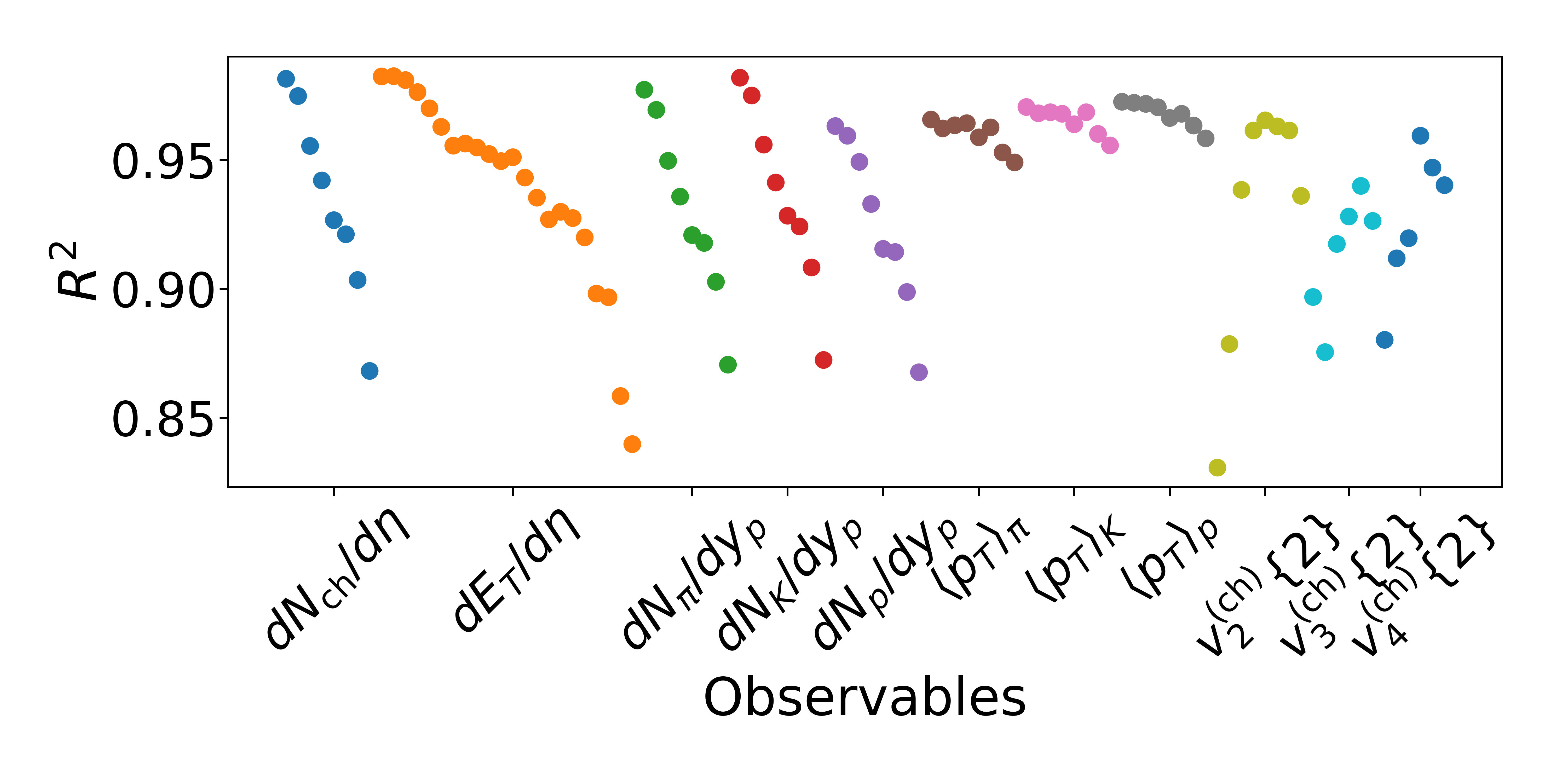
Figure 1: $\mathrm{R}^{2}$ scores calculated using the test simulations and emulator predictions for principal component stochastic kriging (PCSK) for eleven observable types. Each observable type is represented by a unique color, and each dot corresponds to measurements of that observable type at increasing centrality when going from left to right.

Once the emulators are fitted with training data, and before using them for Bayesian parameter inference, we test the accuracy of the emulators. To do that, we use the model simulation output from a batch of $m$ design points that was put aside and not used for emulator training (specifically batch (b) described in App. A). The emulator accuracy is measured using the coefficient of determination ($R^{2}$ score) for the $l^{\mathrm{th}}$ observable ($l=1,\ldots,d$) defined by

$$R^{2}_{l}=1-\frac{\sum_{i=1}^{m}(\bar{\mathbf{y}}_{{\rm sim},l}(\mathbf{x}_{i}^{\rm test})-\boldsymbol{{\mu}}_{l}(\mathbf{x}_{i}^{\rm test}))^{2}}{\sum_{i=1}^{m}(\bar{\mathbf{y}}_{{\rm sim},l}(\mathbf{x}_{i}^{\rm test})-\bar{\bar{\mathbf{y}}}_{{\rm sim},l}(\mathbf{x}_{i}^{\rm test}))^{2}}\,,$$ (25)

$${\rm where}\quad\bar{\bar{\mathbf{y}}}_{{\rm sim},l}(\mathbf{x}_{i}^{\rm test})=\frac{\sum_{i=1}^{m}\bar{\mathbf{y}}_{{\rm sim},l}(\mathbf{x}_{i}^{\rm test})}{m}.$$

The maximum possible value for $R_{l}^{2}$ is $R_{l}^{2}{\,=\,}1$, which occurs only when the emulation predictions for observable $l$ are identical to the simulation output for all $m$ test designs (i.e., the emulator is perfect on the test designs). The $R^{2}$ score can assume negative values when the emulator predictions deviate strongly from the simulation outputs for the test designs.

The $R^{2}$ scores we obtain for the VAH emulators trained by using the principal component stochastic kriging (PCSK) method

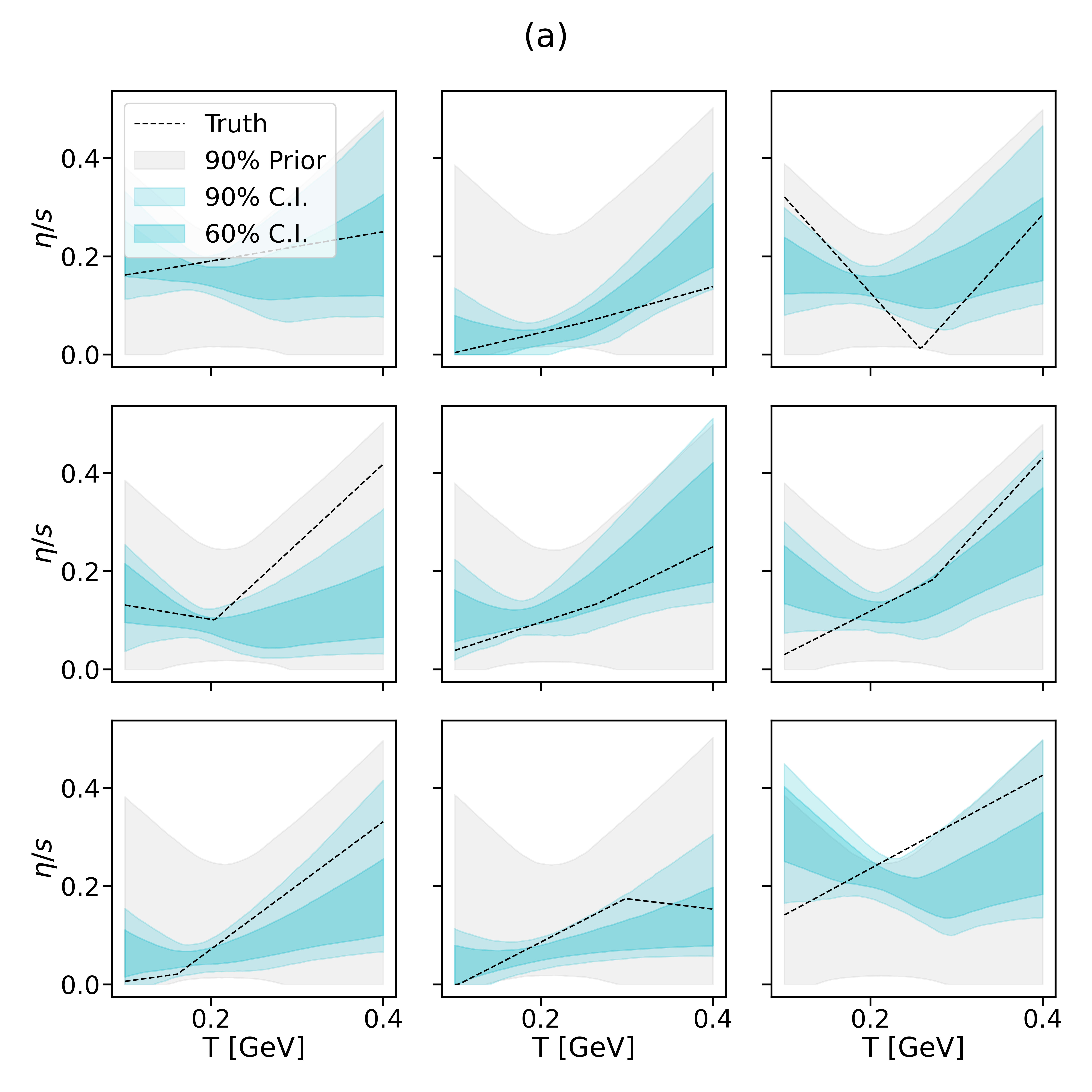
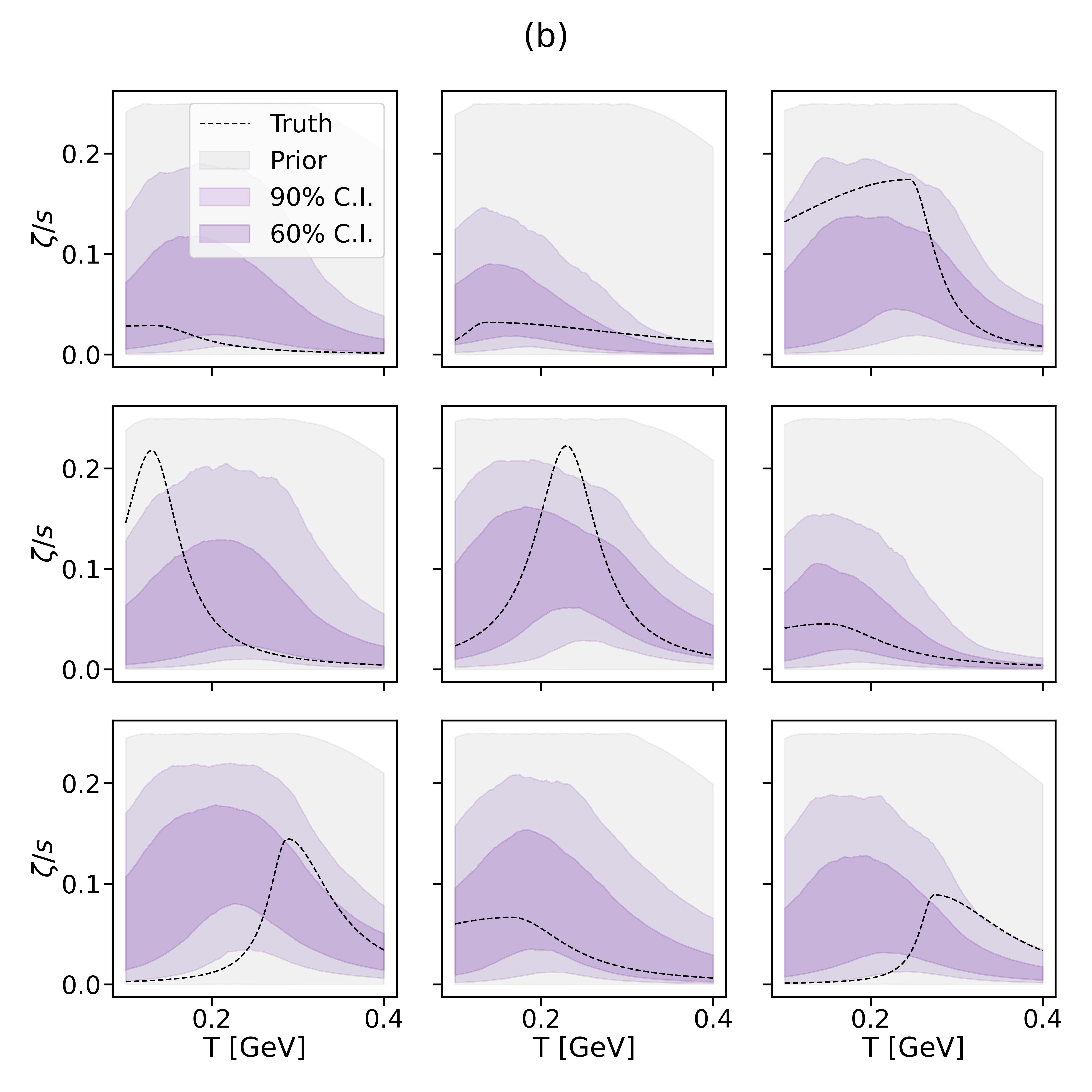
Figure 2: Closure tests for the temperature-dependent specific (a) shear and (b) bulk viscosities. The colored bands show different confidence intervals (C.I.).

are shown in Fig. 1. Each color corresponds to a different type of observable, and each dot corresponds to a different collision centrality, ordered from left to right by increasing centrality. In total there are 98 dots, corresponding to the 98 observables considered in this work.

V Closure tests

Following Ref. Everett et al. (2021b), we perform closure tests before proceeding to the model calibration stage. By using Bayesian inference to reconstruct the model parameters from simulated (“mock”) data generated by model runs for a known point in model parameter space, closure tests are an important check of the ability of the inference framework to correctly infer model parameters from real experimental measurements, and they also provide a deeper understanding of the behavior of the uncertainties associated with the inference process.

We randomly pick nine design points from our most accurate simulation data set (batch (e) in App. A), which has 1600 events per design. We train our emulators without including these nine design points in our training data. Then, the simulation outputs of these nine design points are taken as pseudo-experimental data and we perform the Bayesian parameter inference to find the most probable values of the model parameters that can reproduce the pseudo-experimental data. Finally, we compare the inferred model parameter values with the known truth values that generated these pseudo-experimental data and validate our Bayesian parameter estimation framework.

Figure 2 shows the closure test results for the temperature-dependent specific bulk and shear viscosities. One sees that in most of the nine cases the true model parameter values (giving rise to the dotted lines) are well captured by the 90% inferred posteriors for these model parameters (indicated by lighter and darker colored regions for the 90% ad 60% confidence intervals (C.I.), respectively). We expect the true value (black dashed line) to lie inside the 90% confidence interval 90% of the time. We also observe that for some pseudo-experimental data values (e.g., left column, middle row in both panels (a) and (b)) the closure can be poor. There are several possible reasons for this to happen: a) emulators are not well trained to capture the simulation behavior around some of the parameter values used to generate pseudo-experimental data; b) in some regions of the parameter space the temperature-dependent viscosities are not sensitive enough to be accurately inferred using the currently used experimental observables; a similar issue was reported in Section V.B of Ref. Heffernan et al. (2023). The observation of such instances of poor closure highlights the importance of further validation tests after completing the model calibration. For this purpose we perform posterior predictive tests for the experimental data as discussed in Sec. VIII. For the closure tests shown here, in addition to the viscosities we also checked the consistency of the posteriors for the remaining model parameters with their true values; we found all of them to be inferred accurately.

VI Bayesian calibration of VAH with LHC data

VI.1 Calibration procedure

With our Bayesian tool set in place we perform Bayesian parameter inference using experimental data for Pb–Pb collisions at center-of-mass energy $\sqrt{s_{\textrm{NN}}}{}=2.76$ TeV collected at the LHC. For ease of comparison, we use (almost) the same set of measurements as the recent JETSCAPE analysis Everett et al. (2021b) (98 measurements in total):

• the charged particle multiplicity $dN_{\text{ch}}/d\eta$ Aamodt et al. (2011a) for centrality bins covering $0{-}70$% centrality;

• the transverse energy $dE_{T}/d\eta$ Adam et al. (2016) for centrality bins covering $0{-}70$% centrality;

• the multiplicity $dN/dy$ and mean transverse momenta $\langle p_{T}\rangle$ of pions, kaons, and protons Abelev et al. (2013) for centrality bins covering $0{-}70$% centrality;

• the two-particle cumulant harmonic flows $v_{n}\{2\}$ $(n{\,=\,}2,3,4)$ for centrality bins covering $0{-}70$% centrality for $n{\,=\,}2$ and $0{-}50$% centrality for $n{\,=\,}3,\,4$ Aamodt et al. (2011b).

The 15 model parameters that we infer and their priors are listed in Table 1. Since VAH has no free-streaming stage, the associated JETSCAPE parameters are missing from the table. The additional parameter $R{\,\in\,}[0.3,\,1]$, defined in Eq. (13), controls the initial pressure anisotropy $(\mathcal{P}_{L}/\mathcal{P}_{L})_{0}$ and is unique to VAH.

parameter	prior range
$N$	$[10,30]$
$p$	$[-0.7,0.7]$
$w$ [fm]	$[0.5,1.5]$
$d_{\mathrm{min}}$ [fm]	$[0.0,1.7]$
$\sigma_{k}$	$[0.3,2.0]$
$T_{\mathrm{sw}}$ [GeV]	$[0.135,0.165]$
$R$	$[0.3,1]$
$T_{\eta/s,\mathrm{kink}}$ [GeV]	$[0.13,0.3]$
$(\eta/s)_{\rm kink}$	$[0.01,0.2]$
$a_{\mathrm{high}}$ [GeV-1]	$[-1,2]$
$a_{\mathrm{low}}$ [GeV-1]	$[-2,1]$
$(\zeta/s)_{\mathrm{max}}$	$[0.01,0.25]$
$T_{\zeta}$ [GeV]	$[0.12,0.3]$
$w_{\zeta}$ [GeV]	$[0.025,0.15]$
$\lambda_{\zeta}$	$[-0.8,0.8]$

Table 1: List of VAH model parameters. We use uniform priors throughout, with prior ranges (specified in the right column) that agree with the ones used in Ref. Everett et al. (2021b).

For the likelihood function we use the multivariate normal distribution (19). The variances characterizing the experimental and simulation uncertainties are added together to obtain the total uncertainty appearing in the likelihood.

The posterior is found by combining the (multivariate Gaussian) likelihood with the (multivariate uniform) prior according to Bayes’ rule (18). The resulting 15-dimensional posterior probability distribution is analyzed by sampling it using MCMC Peters (2008); Trotta (2008b). Specifically, we use the Parallel Tempering MCMC technique Vousden et al. (2015); Foreman-Mackey et al. (2013); pte , on account of its robustness in sampling multi-modal posterior distributions. For the temperature ladder we choose 500 values for the tempering temperature, evenly distributed between 0 and 1000. For each temperature in the ladder we run 100 randomly initialized chains (see pte for technical details of the parallel tempering algorithm). In each chain we discard the first 1000 steps as burn-in. The final posterior samples are obtained from the next 5000 steps, after thinning the chains by a factor 10, by saving only every 10th sample.

VI.2 Posterior for the model parameters

The joint marginal posterior distributions (obtained by projecting the posterior on two dimensions in all possible ways) for all the model parameters are shown in Fig. 3; the diagonal shows the marginal posterior distributions for each model parameter. These marginal distributions are obtained by integrating the posterior over all other model parameters, except the chosen one or two. The model parameter values that maximize the high-dimensional posterior (the “mode” of the distribution) are called Maximum a Posteriori (MAP) parameters — they are indicated by blue dotted vertical lines in the diagonal panels.

In each panel the lilac color shades the uniform prior distribution density; shades of red color indicate the projected density of the posterior distribution. In cases where the available experimental data have insufficient constraining power on a parameter one expects the prior (blue) and posterior (red) marginal distributions to largely agree. In these cases the posterior essentially returns the information already contained in the prior. Figure 3 shows that two of our model parameters related to the very early stage of the fireball, the initial pressure ratio $R$ and the minimum distance $d_{\mathrm{min}}$ between nucleons, are not well constrained by the experimental data.

Figure 3: Joint marginal distributions of the posterior for all model parameters, for VAH with PTMA viscous corrections at particlization and using experimental data from Pb–Pb collisions at $\sqrt{s_{\textrm{NN}}}{}=2.76$ TeV. Posterior distributions are represented by shades of red while the (uniform) prior distributions are shown in lilac. Cyan numbers and vertical dotted lines in the diagonal panels indicate the MAP values for each parameter. (See Table 1 for the units of the model parameters.)

The shape of the probability density contours in the off-diagonal panels conveys information about correlations among the inferred model parameters. When considering parameters unrelated to the viscosities one observes slight positive correlations between the nucleon width parameter $w$, as well as the multiplicity fluctuation parameter $\sigma_{k}$, and the T_RENTo normalization $N$, and between $\sigma_{k}$ and the minimum nucleon distance $d_{\mathrm{min}}$; the power $p$ in the T_RENTo parameterization (4) of the reduced thickness function $T_{R}$ is slightly anti-correlated with $N$ and $R$. More striking is the bimodal structure of the T_RENTo normalization parameter $N$. In all previous Bayesian parameter inferences for heavy-ion collision simulations for Pb–Pb at $\sqrt{s_{\textrm{NN}}}{}=2.76$ TeV energy, the marginal distribution of $N$ was well constrained to a Gaussian-like distribution Petersen et al. (2011); Novak et al. (2014); Sangaline and Pratt (2016); Bernhard et al. (2015, 2016); Moreland et al. (2020); Bernhard et al. (2019); Everett et al. (2021a); Nijs et al. (2021a, b); Everett et al. (2021b). Since $N$ determines the initial energy deposited after the collision, it is also closely related to the initial entropy. This causes the final particle yields to directly scale with $N$. Using primarily the final measured particle yields and transverse energy, all previous Bayesian studies were able to tightly constrain $N$. The deviation from this in the VAH model warrants further investigation into the sub-dominant peak that appears at higher $N$ values closer to the prior bound.

As a first step towards understanding the bimodal structure, we look at all the correlations seen in the joint marginal distributions between $N$ and the other model parameters, shown in the leftmost column of Figure 3. Five parameters are seen to correlate most strongly with the two peaks in the marginal posterior for $N$: $p$, $w$, $\sigma_{k}$, $a_{\mathrm{high}}$, and $R$ all prefer different values for the two peaks of $N$. This suggests that one of these parameters, or some combination of them, acts to compensate the effect that a large $N$ value has on the final observables.

To narrow things down further requires going beyond the pairwise joint marginal posterior distributions. We therefore jump ahead to the model sensitivity shown in Fig. 5 which will be discussed in greater detail in Sec. VII below. Figure 5 shows that the charged particle yields for central collisions show significant sensitivities only to $N$ and the specific shear viscosity $\eta/s$. Further checking along these lines points to the possibility that the two-peak structure in $N$ might be related specifically to the high-temperature slope of the specific shear viscosity, $a_{\mathrm{high}}$.

Closer inspection of the joint marginal distribution between $a_{\mathrm{high}}$ and $N$ in Figure 3 shows that these two parameters are anti-correlated. The peak at large $N$-values correlates with negative slope $a_{\mathrm{high}}<0$ (i.e. a specific shear viscosity that decreases with temperature) whereas $a_{\mathrm{high}}>0$ (i.e. $\eta/s$ increases with temperature) for smaller values of $N$.

The VAH model starts the hydrodynamic evolution at the very early time of $\tau_{0}=0.05$ fm/$c$, thus probing much higher temperatures than any other hydrodynamic model for heavy-ion collisions used so far. Smaller (but still positive) high-temperature values of $\eta/s$ result in reduced viscous heating during the earliest evolution stage and, therefore, in lower final particle yields as well as smaller mean transverse momenta and flow anisotropies. To hold these observables constant as $N$ increases, the Bayesian fit compensates by reducing the specific shear viscosity in particular at early times (i.e. at high temperature) when the rate of viscous entropy production is largest. This is accomplished by selecting a negative slope parameter $a_{\mathrm{high}}$. This unique characteristic of the VAH model explains the bimodal structure of the marginal posterior for $N$ which has not been observed in any other model for heavy-ion collisions. We note that a similar bimodal structure is also seen in the joint marginal distributions of several other parameter pairs but hidden in their individual marginal distributions.

For the VAH model the MAP value for the harmonic mean parameter $p$ in T_RENTo (see Eq. (4)) is 0.038, close to the preferred value of zero found in all previous Bayesian parameter inferences using a free-streaming pre-hydrodynamic stage Petersen et al. (2011); Novak et al. (2014); Sangaline and Pratt (2016); Bernhard et al. (2015, 2016); Moreland et al. (2020); Bernhard et al. (2019); Everett et al. (2021a); Nijs et al. (2021a, b); Everett et al. (2021b). However, its marginal posterior distribution is shifted toward slightly negative values. Its correlation with $N$ suggests that this shift is associated with the large posterior density around negative values of $a_{\mathrm{high}}$, which we argued above corresponds to small specific shear viscosity values at early times. The small specific shear viscosity causes the fluid to behave more ideal, quickly erasing all initial momentum anisotropies and thereby reducing all finally measured flow harmonics. To compensate for this effect the harmonic mean parameter $p$ tends negative, which, as observed in Moreland et al. (2015) and confirmed with the VAH widget in Liyanage , increases all flow harmonics. Decreasing the specific shear viscosity also correlates with a growth of the multiplicity fluctuation parameter $\sigma_{k}$, compensating for the faster decay of initial momentum anisotropies with larger initial density fluctuations to keep the final anisotropic flow response strong.

We note that the marginal posterior peak at the larger $N$ values correlates not only with a reduced specific shear viscosity at high temperatures, but also with a large value $R\approx 1$ of the initial pressure ratio $P_{L}/P_{\perp}$ (i.e. a small value for the initial shear stress). We point out that the degeneracy in probability between the two peaks seen in the marginal posterior for $R$ can be broken, at the level of the prior distribution for $R$, by invoking additional “prior theoretical” input: In the widely considered Color Glass Condensate (CGC) model Gelis et al. (2010), which is expected to apply to heavy-ion collisions at LHC energies, the longitudinal pressure $P_{L}$ is predicted to be initially negative, rising very quickly (on a time scale ${\sim\,}1/Q_{s}$ where $Q_{s}{\,\sim\,}1{\,-\,}3$ GeV is the saturation momentum of the CGC) to positive values and approaching the transverse pressure $P_{\perp}$ from below at late times as the system moves closer to thermal equilibrium Epelbaum and Gelis (2013). This picture would definitely tilt the prior for $R$ in the lower right panel of Fig. 3 strongly toward the left, assigning very low prior (and therefore also posterior) probability to initial pressure ratios near $R{\,=\,}1$.

Similar to earlier Bayesian model calibrations Moreland et al. (2020); Bernhard et al. (2019); Nijs et al. (2021a); Everett et al. (2021b); Nijs and van der Schee (2022a) we find the nucleon width parameter $w$ constrained to a value around 1 fm. Since this value is larger than the nucleon width needed to match the recently measured total hadronic cross sections for $p$–Pb Khachatryan et al. (2016) and Pb–Pb ALICE-Collaboration (2022) collisions at $\sqrt{s_{\textrm{NN}}}{\,=\,}5.02$ GeV at the LHC Nijs and van der Schee (2022b), this suggests that a successful description of the experimental data used in our model calibration requires an initial density profile (3) for the energy density deposited near mid-rapidity that fluctuates on a larger length scale than the strong interaction radius of the proton. The VAH widget Liyanage (see footnote 14) shows that bumpier initial conditions whose density fluctuates on shorter length scales increase the radial and anisotropic flows (reflected in the average momenta $\langle p_{T}\rangle$ and harmonic flow coefficients $v_{n}$ of the emitted hadrons) which must be compensated by larger values for the shear and bulk viscosities. Thus, the choice of $w$ has direct consequences for the viscosity coefficients inferred from the experimental data.

The fluctuation length scale of the initially deposited matter should be larger than that of the nuclear thickness functions of the colliding nuclei makes immediate sense once one realizes that the matter created by a collision of two colored partons at transverse position $\mathbf{x}_{\perp}$, which is characterized by a typical transverse momentum scale $p_{\perp}{\,\lesssim\,}1$ GeV, cannot be deposited at precisely the same point $\mathbf{x}_{\perp}$: the uncertainty relation requires it to be distributed around $\mathbf{x}_{\perp}$ in a cloud of transverse radius $\Delta r_{\perp}{\,\sim\,}\mathcal{O}(1/p_{\perp})$. Unfortunately, the T_RENTo ansatz (3,4) does not

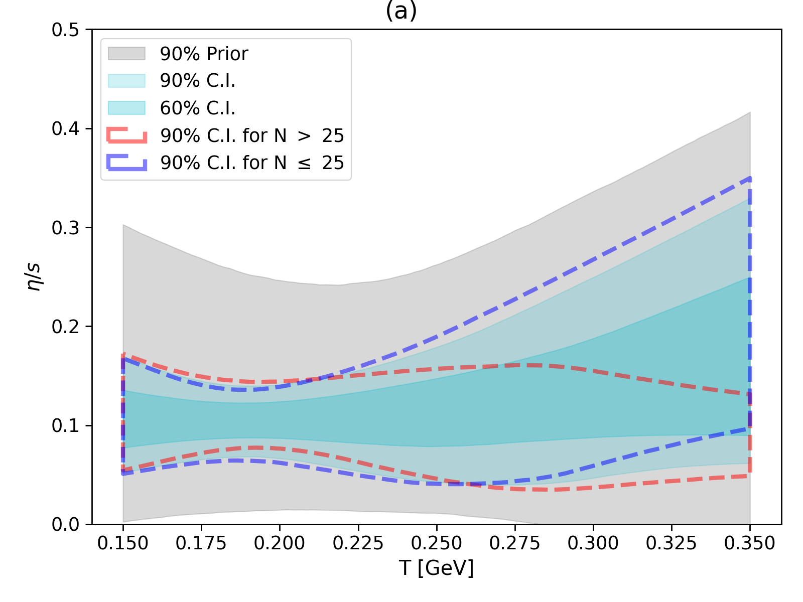
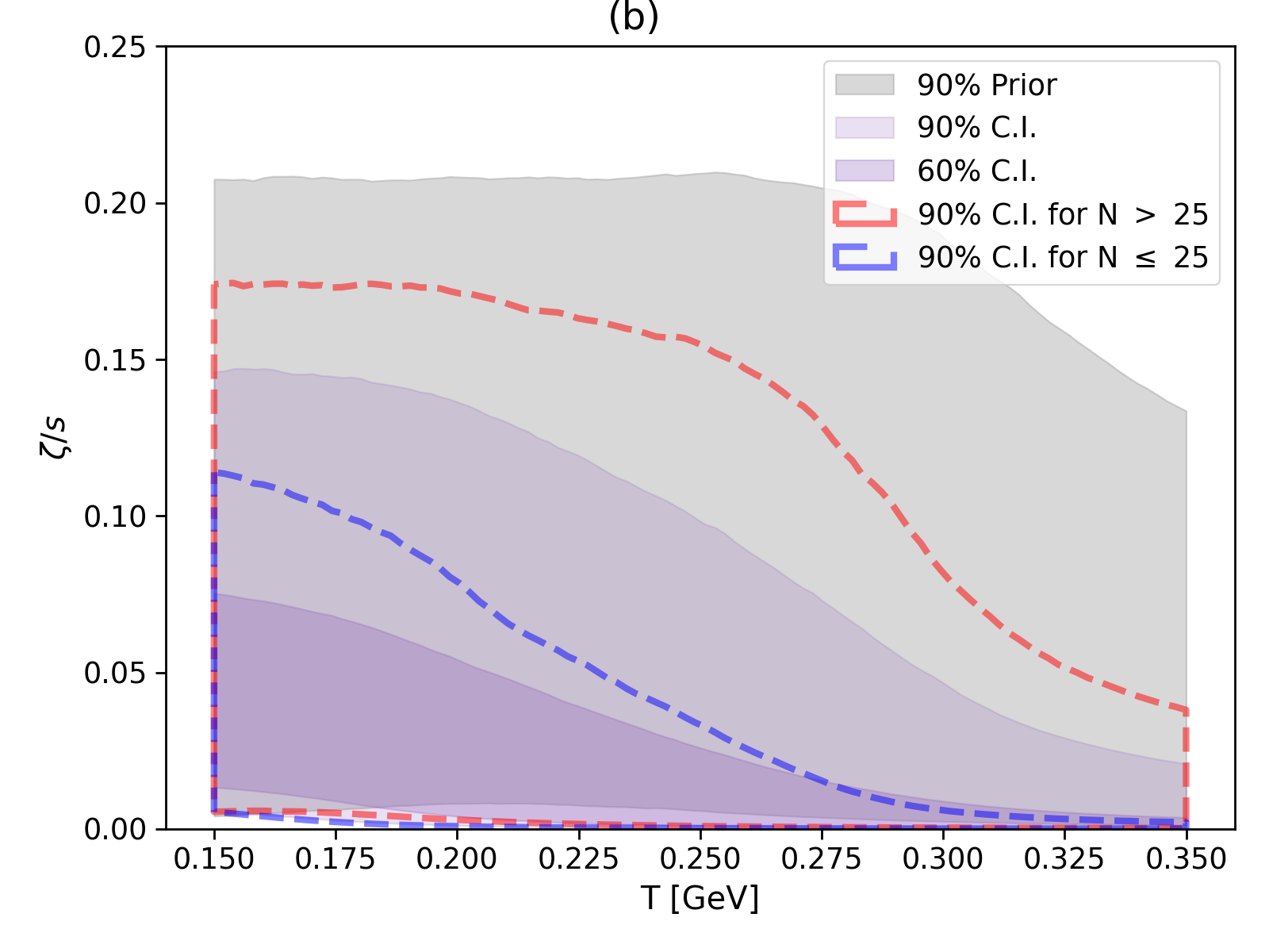
Figure 4: Posteriors for the temperature-dependent specific (a) shear and (b) bulk viscosities in the VAH model with PTMA viscous corrections at particlization, using experimental data from Pb–Pb collisions at $\sqrt{s_{\textrm{NN}}}{}=2.76$ TeV for model calibration. Grey bands show the 90% prior interval. The colored regions corresponds to 90% (light) and 60% (dark) posterior credible intervals. Dashed lines indicate the 90% posterior credible intervals within the parameter subspaces corresponding to T_RENTo normalization $N>25$ (red) and $N\leq 25$ (blue), respectively. See text for discussion.

allow to change the width parameter $w$ independently in the nuclear thickness functions $T_{A,B}$ (which control, among other observables, the total inelastic $p$–Pb and Pb–Pb cross sections Khachatryan et al. (2016); ALICE-Collaboration (2022); Nijs and van der Schee (2022b)) and in the reduced thickness function $T_{R}$ (4) which controls the fluctuation length scale of the initially deposited transverse density profile. We suggest that future implementations of the T_RENTo model should allow for an additional Gaussian smearing in Eq. (3),

$$\epsilon(\mathbf{x}_{\perp})=\frac{N}{\tau_{0}}\int d^{2}r_{\perp}T_{R}(\mathbf{r}_{\perp};p,w)\,\frac{e^{-\frac{1}{2}\bigl{(}\frac{\mathbf{x}_{\perp}{-}\mathbf{r}_{\perp}}{\Delta r_{\perp}}\bigr{)}^{2}}}{2\pi(\Delta r_{\perp})^{2}},$$ (26)

where $T_{R}$ is characterized by a nucleon width $w$ matched to reproduce the total inelastic $p$–Pb and Pb–Pb cross sections Nijs and van der Schee (2022b) while the additional smearing scale $\Delta r_{\perp}$, setting the length scale of the initial energy density fluctuations, is taken as a model parameter to be inferred from the heavy-ion collision data by Bayesian inference.

Our Bayesian model calibration leaves the minimum distance $d_{\mathrm{min}}$ between nucleons unconstrained. This has also been observed in other Bayesian parameter estimation studies done with the T_RENTo model Everett et al. (2021b). The switching temperature $T_{\mathrm{sw}}$ where the QGP is converted into hadrons is constrained to a somewhat lower temperature than in previous studies Everett et al. (2021b); Nijs et al. (2021a). While its MAP value $T_{\mathrm{sw}}^{\mathrm{MAP}}=146$ MeV is compatible with earlier analyses, its marginal posterior is tilted toward lower temperatures and abuts the lower edge of its prior interval. This shift toward lower particlization temperatures suggests that the very tight constraints for $T_{\mathrm{sw}}$ observed in earlier Bayesian analyses using different evolution models are affected by significant model uncertainties, and that in future Bayesian parameter studies with the VAH model the prior for this parameter should be extended toward lower temperature values.

VI.3 Posteriors for the temperature-dependent specific shear and bulk viscosities

The posterior probability distributions for the temperature-dependent specific shear and bulk viscosities of the QGP, inferred from experimental data for Pb–Pb collisions at $\sqrt{s_{\textrm{NN}}}{}=2.76$ TeV, are shown in Fig. 4.

Comparing with two other recent Bayesian parameter studies Everett et al. (2021b); Nijs et al. (2021a) we observe improved posterior constraints especially in the upper temperature range. The specific bulk viscosity is constrained to very low values ($\zeta/s{\,<\,}0.01$ with 60% confidence) at temperatures above 350 MeV; at temperatures below 220 MeV the constraints are similar to those in Ref. Everett et al. (2021b). For the specific shear viscosity $\eta/s$ we find posterior constraints that again are consistent with previous Bayesian parameter inference studies at temperatures below 250 MeV, but are much tighter and weighted toward lower $\eta/s$ values at higher temperatures when using VAH than found with the earlier models that assumed a free-streaming pre-hydrodynamic stage.

The better constraints at higher temperatures make sense when noting that in our VAH model the specific bulk and shear viscosities enter as model parameters into the description of the dynamical evolution at much earlier times, when the energy density (which controls the associated equilibrium temperature by Landau matching) is much higher. In the JETSCAPE Everett et al. (2021b) and Trajectum Nijs et al. (2021a) models $\eta/s$ and $\zeta/s$ do not enter until the beginning of the viscous hydrodynamic stage after about 1 fm/$c$ or later, when the energy density has already dropped by a factor 20 or more, corresponding to a decrease by more than factor 2 in temperature. The initial free-streaming stage assumed in Refs. Everett et al. (2021b); Nijs et al. (2021a) can in fact be thought of as a fluid with infinite shear and bulk viscosities. The present work shows that by replacing the unphysical free-streaming stage by viscous anisotropic hydrodynamics we can achieve a description of the experimental measurements that is at least as good as achieved in the previous model calibrations (see further discussion below) and which allows us to probe the temperature dependence of the QGP viscosities to much higher temperatures than possible before. An additional benefit of the VAH approach is that it eliminates the unphysical switching time from free-streaming to hydrodynamics as a model parameter, and also avoids the large and positive (i.e., wrong-signed) artificial starting values of the bulk viscous pressure that arise from matching the conformal free-streaming stage to a hydrodynamic fluid with a realistic, non-conformal EoS.

In Section VI.2 we found that the entropy generated by viscous heating drives the unique bimodal structure seen in the posterior shown in Fig. 3. The dashed lines in Fig. 4 provide additional support for our analysis: In order to identify the contribution from each of the two modes to the final posteriors for the temperature dependent viscosities, we divide the 15-dimensional parameter space into subspaces with T_RENTo normalization parameter $N>25$ and $N\leq 25$. The red and blue dashed lines in Fig. 4 delineate the corresponding 90% posterior credible intervals for the specific viscosities when the range of $N$ is restricted in this way to capture one or the other of these two modes.

For large initial entropy ($N{\,>\,}25$) the specific shear viscosity $\eta/s$ is seen to most likely remain small (close to $1/4\pi$) as the temperature increases, thereby suppressing additional shear viscous entropy production during the earliest and hottest expansion stage. For small initial entropy deposition ($N{\,\leq\,}25$), $\eta/s$ rises with increasing temperature, entailing significant shear viscous heating during the hottest earliest stage. Panel (b) shows that complex constraints provided by the experimental data correlate an increase of the shear viscosity $\eta/s$ at high $T$ with a concomitant decrease of the bulk viscosity $\zeta/s$, and vice versa. The model sensitivity analysis in the next section reveals an overall rather weak sensitivity of the observables used for model calibration to the bulk viscosity $\zeta/s$: only the proton yield and the pion and proton $\langle p_{T}\rangle$ respond significantly to changes in $\zeta/s$, but at the same time they respond much more strongly to several other model parameters. The anti-correlation between $\eta/s$ and $\zeta/s$ at high temperature seen in Fig. 4 when comparing the regions encircled by the dashed red and blue lines is therefore likely caused by a combination of several small effects that requires retuning multiple parameters simultaneously in the VAH widget Liyanage .

VII Model sensitivity

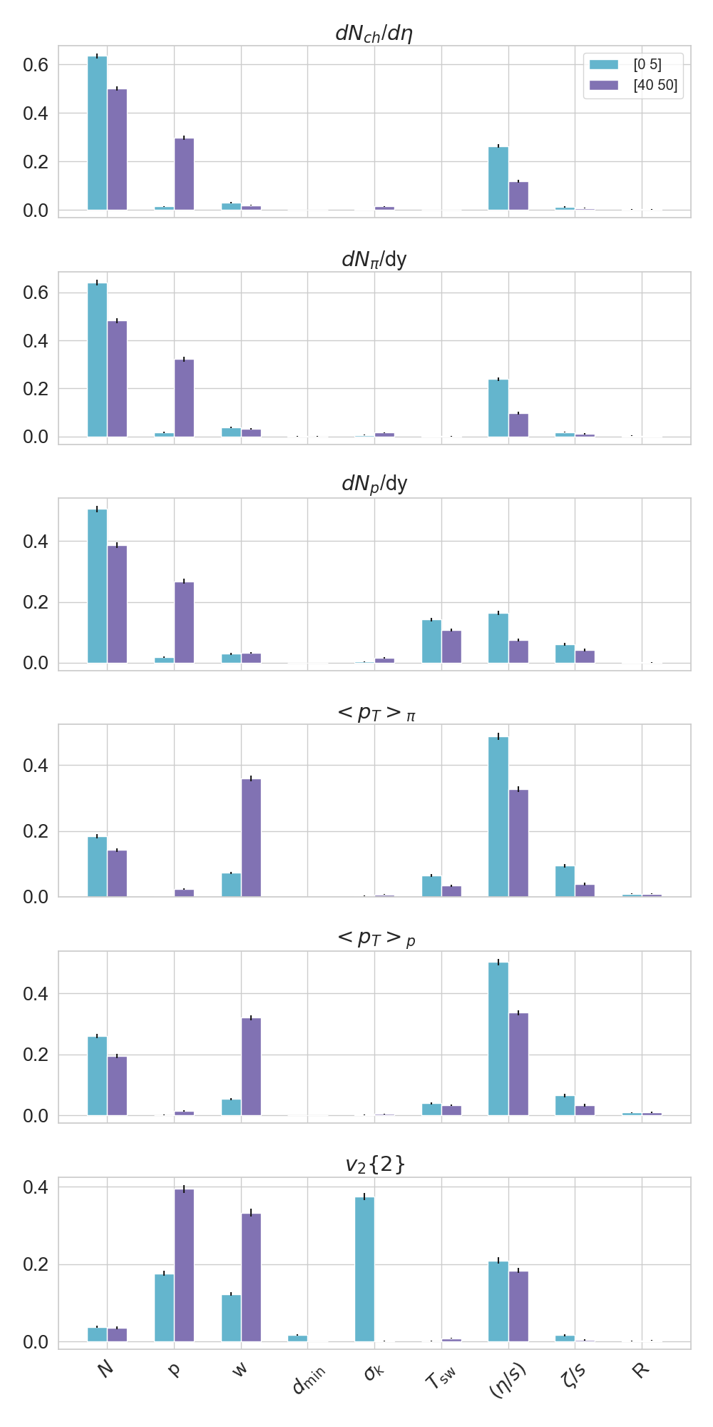
Figure 5: First-order Sobol’ sensitivities (App. D) for the VAH model.

In this section, we perform a sensitivity analysis on our model emulators to understand how the VAH model observables respond to changes in the model parameters. The first-order Sobol’ sensitivity analysis performed here measures the global sensitivity of the model to its parameters Sobol’ (1990); Liyanage et al. (2022). Here we have grouped the parameters related to shear and bulk viscosity into two separate groups and measure the overall sensitivity of the model to these grouped sets for the ease of presentation Jacques et al. (2006); see App. D for details.

Figure 5 shows the first-order Sobol’ sensitivity indices calculated for 6 types of observables for the VAH model. The blue color is for observables measured in the most central collisions (0-5% centrality) while the purple color represents observables in the mid-centrality range (40-50% centrality).

We observe that charged and identified particle yields for pions and protons are mostly sensitive to the T_RENTo normalization, $N$. The normalization directly scales the magnitude of the initial energy deposition profile from T_RENTo and thus controls the number of particles produced at freeze out. Interestingly, we find that the charged particle and pion yields display their second strongest sensitivity to the grouped specific shear viscosity $\eta/s$. Further exploration reveals that this sensitivity is caused by viscous heating effects during the fireball evolution, especially at very early times. We invite the interested reader to further verify this by using the VAH widget link in footnote 14. In the widget, reducing the high temperature slope of the specific shear viscosity, keeping everything else fixed, results in a dramatic decrease of the charged particle and pion yields, showing the effect of viscous heating. This strong sensitivity is a specific feature of VAH which starts the (anisotropic) hydrodynamic evolution very early (from 0.05 fm/$c$) when the temperature is high, providing a strong lever arm for the slope parameter $a_{\mathrm{high}}$.

The same observables measured in peripheral collisions, but not in central collisions, are sensitive to the T_RENTo harmonic mean parameter $p$, which controls how the nucleon thickness functions for each of the nucleus are combined to produce the initial energy profile.

The mean transverse momenta of both pions and protons are most sensitive to the grouped specific shear viscosity parameters, with somewhat weaker sensitivity to the normalization parameter $N$. The same observables also have high sensitivity to the nucleon width $w$ measured in peripheral collisions but not in central collisions.

The elliptic flow observables measured in the most central collisions exhibit the strongest sensitivity to the multiplicity fluctuation parameter $\sigma_{k}$. The average shape of the nuclear overlap region being perfectly azimuthally symmetric in the most central collisions, flow anisotropies arise only from event-by-event fluctuations in these collisions, explaining their sensitivity to $\sigma_{k}$. The elliptic flow also shows unsurprisingly significant sensitivities to the grouped specific shear viscosity parameters and the T_RENTo parameters $p$ and $w$, in both central and peripheral collisions. The latter again reflects the roles of these parameters in the event-by-event fluctuation spectrum characterizing the initial conditions.

None of the selected observables exhibit any appreciable sensitivity to the initial pressure anisotropy parameter $R$ or the minimum distance $d_{\mathrm{min}}$ between nucleons when sampling their positions from the Woods-Saxon distribution. This observation is consistent with the very broad marginal posteriors for these two parameters shown in Fig. 3. These suggest that additional novel observables (to sharpen their marginal posteriors) and/or trustworthy additional theoretical arguments (to better constrain their priors) are needed to better constrain these model parameters.

In Ref. McNelis (2021) the author tried to keep all except two parameters in the VAH model fixed at the MAP values of the recently calibrated JETSCAPE SIMS model Everett et al. (2021b), seeking VAH values only for the normalization $N$ and nucleon width $w$. The resulting fit McNelis (2021) agreed surprisingly well with the experimental data. The above sensitivity can explain this unexpected success: Fig. 5 shows that $N$ and $w$ are the two parameters to which most of the selected observables exhibit significant sensitivity, so adjusting them captures most of the variation of the observables under model parameter change. For this reason we have also included the VAH parameter set proposed in McNelis (2021) as their “best guess" as one of our design points when training emulators.

Our trained emulators for the VAH model can be accessed by following the link in footnote 14 and Ref. Liyanage . The “VAH widget” produces the centrality dependent observables in real time for any model parameter values within their prior bounds. As long as only model predictions for the set of experimental data used in the VAH calibration are desired, the widget can serve as a fast and quantitatively precise emulator of the full VAH model. We found it very useful for developing intuition for the response of the observables to changes in single or combinations of model parameters. While no substitute for the full solution of the “inverse problem” (i.e., the inference of the model parameters from the observables), it can help to develop an in-depth understanding of such a solution.

VIII Predictions from the maximum a posteriori probability

The final result of the Bayesian parameter estimation work presented here are computationally cheap samples of the experimental observables from the most probable region in the multidimensional posterior distribution for the model parameters. To visualize and understand the full posterior distribution we have used plots of the 1- and 2-dimensional (single or joint) marginal distribution in Figs. 3 and 4. In this section we will show how to find a point estimate from the posterior, i.e., the set of model parameters that can best fit the experimental data. The comparison between the simulation predictions for this set of model parameter values (the MAP values) and the experimental measurement will be a final test for the validity of the Bayesian parameter inference framework that we have used in this work. We note, however, that model predictions that quantitatively include the full uncertainty range arising from the uncertainties of the inferred model parameters require a posterior-weighted sample from the entire high-probability region in the multidimensional parameter space.

parameter	MAP values
$N$	$20.013$
$p$	$0.038$
$w$ [fm]	$0.985$
$d_{\mathrm{min}}$ [fm]	$0.878$
$\sigma_{k}$	$1.184$
$T_{\mathrm{sw}}$ [GeV]	$0.146$
$R$	$0.653$
$T_{\eta/s,\mathrm{kink}}$ [GeV]	$0.219$
$(\eta/s)_{\mathrm{kink}}$	$0.094$
$a_{\mathrm{high}}$ [GeV-1]	$0.493$
$a_{\mathrm{low}}$ [GeV-1]	$-0.383$
$(\zeta/s)_{\mathrm{max}}$	$0.044$
$T_{\zeta}$ [GeV]	$0.235$
$w_{\zeta}$ [GeV]	$0.032$
$\lambda_{\zeta}$	$0.037$

Table 2: Model parameters corresponding to the mode of the posterior distribution (MAP) for the VAH model. These model parameters provide simulation outputs that agree best with the experimental measurements.

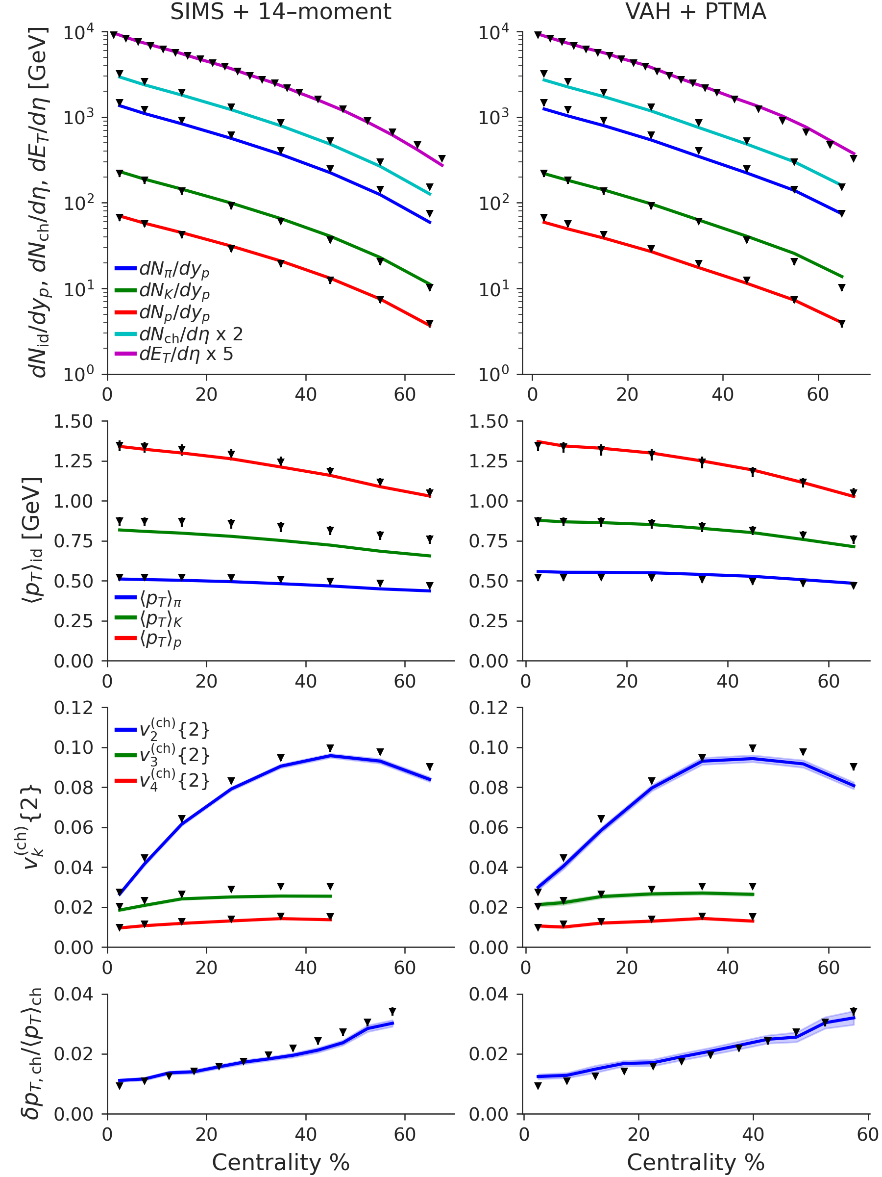
Figure 6: MAP predictions for the JETSCAPE SIMS model with Grad 14-moment viscous corrections at particlization from Ref. Everett et al. (2021b) (left column) compared with those for the VAH model with PTMA viscous corrections at particlization (right column).

The model parameters that correspond to the mode of the posterior distribution are called maximum a posterior probability (MAP) values. The MAP values are found using numerical optimization algorithms that find the model parameter values that minimize the negative log posterior distribution Storn and Price (1997); Virtanen et al. (2020). The MAP values for the posterior obtained in this work are listed in Table 2.

In Fig. 6 we compare how the MAP prediction from the VAH model compares with another recent Bayesian parameter estimation study published in Ref. Everett et al. (2021b). The left column of Fig. 6 is obtained by using the JETSCAPE SIMS model Everett et al. (2021b) with its MAP parameter values and running 3000 events with fluctuating initial conditions. The right column is obtained by the same procedure using the VAH model with its MAP parameter set. In both columns the black triangles show the experimental measurements taken with Pb–Pb collisions at the LHC at $\sqrt{s_{\textrm{NN}}}{}=2.76$ TeV. While both fits look good, closer inspection reveals several detailed features in the data that are better described by VAH and none that are significantly better described by JETSCAPE SIMS. It is likely, however, that the two sets of model predictions are statistically consistent with each other once a full sample of the posterior probability distribution is generated. We leave this for a future study aimed at a quantitative comparison between the two models and improved observable predictions obtained by combining the models (and variations of them) with Bayesian model mixing techniques Phillips et al. (2021).

It is important to note that the Bayesian parameter estimation carried out here did not use the experimental data for the transverse momentum fluctuations of charged particles, $\delta p_{T}^{\mathrm{ch}}/\langle p_{T}^{\mathrm{ch}}\rangle$, in the model calibration, nor any model predictions for this observable when training the model emulators. The fact that the MAP values for the VAH model successfully reproduce this observable (bottom right panel in Fig. 6) can be interpreted as a successful prediction of the calibrated VAH model.

IX Conclusions

In this work we performed a Bayesian calibration of a novel relativistic heavy-ion collision model, VAH, which treats the early far-from-equilibrium stage of the collision with viscous anisotropic hydrodynamics that is optimized for the particular symmetries that characterize this stage. The experimental input in this study were data taken with Pb–Pb collisions at $\sqrt{s_{\textrm{NN}}}{}=2.76$ TeV at the LHC. The VAH model can be used from very early times onward (here we use $\tau_{0}{\,=\,}0.05$ fm/$c$), which largely obviates the need for any pre-hydrodynamic evolution at all. This eliminates model parameters and other conceptual uncertainties associated with the free-streaming modeling of the pre-hydrodynamic stage employed in similar analyses that employed standard viscous hydrodynamics to model the QGP.

An important advantage of being able to start the hydrodynamic modeling so much earlier is that transport coefficients enter as parameters of the dynamical description at a stage of much higher energy density and temperature. By using the VAH approach we can therefore constrain the specific shear and bulk viscosities at higher temperatures than accessible in other approaches that invoke an extended pre-hydrodynamic stage modeled microscopically in a way that cannot be meaningfully parameterized by hydrodynamic transport coefficients. We find that within the VAH approach the specific bulk viscosity is well constrained by the LHC data to very low values, $\zeta/s{\,<\,}0.03$ at 90% confidence level and ${\,<\,}0.01$ at 60% confidence level, for temperatures above 350 MeV. Also the specific shear viscosity is more tightly constrained at temperatures above 250 MeV than in previous analyses, with the 60% and 90% confidence intervals both pushed toward lower $\eta/s$ values than before. At lower temperatures below 220 MeV the VAH constraints agree with those obtained from previous Bayesian parameter estimation studies.

The joint marginal posterior distributions for pairs of model parameters exposed a bimodal posterior which, in the case of the T_RENTo normalization $N$, is even visible at the level of the individual marginal posterior. We were able to trace this back to a nontrivial interplay between the initial entropy deposition controlled by $N$ and the additional entropy generated by viscous heating during the subsequent evolution. The Bayesian calibration found two different solutions with similar posterior probabilities, corresponding to different trade-offs between these two mechanisms. The use of VAH exposed the possibility of such a trade-off for the first time since previous hybrid evolution models were not able to explore reliably the large viscous heating effects occurring during the very early evolution stage when the longitudinal expansion rate is huge and the fluid is very far from local thermal equilibrium. VAH is optimized to handle this extreme situation within an adapted hydrodynamic approach. We argued that there may be additional theoretical arguments that, in future Bayesian calibration campaigns, can be implemented by appropriate modification of the prior probability distributions for some of the model parameters, in order to resolve the ambiguity between the two modes exposed in this work.

We demonstrated that the primary mode of the full 15-dimensional posterior parameter probability distribution (i.e., its MAP parameter set) leads to a very good description of the data used in the model calibration, with no significant tensions between the calibrated model and the experimental data. The calibrated VAH model was shown to improve on several features where earlier Bayesian model fits exhibited weaknesses. In particular, the MAP parameters of our calibrated VAH model led to a quite successful prediction of the mean-$p_{T}$ fluctuations, a set of data that was not used in the model calibration on account of its high demand on event statistics but was still correctly predicted by the model after calibration with other, statistically less demanding experimental observables.

The comparison of our results here with those obtained earlier with different variants of the heavy-ion collision evolution model shines a light on model uncertainties and their effects on the uncertainty ranges for the fireball parameters inferred with these models from the experimental data. While state-of-the-art Bayesian analyses provide principled uncertainty quantification given the known experimental uncertainties, there is nothing principled about the way the heavy-ion community presently tries to assess theoretical and modeling uncertainties. The availability of several Bayesian calibrated heavy-ion evolution models now opens the window to, and underlines the urgency for developing new statistical tools that enable principled uncertainty quantification in Bayesian model parameter inference that accounts for experimental and theoretical uncertainties on an equal footing.

Appendix A Details of training data collection procedure

The following are, in chronological order, the five batches of design points for which we ran full model simulations.

1. We start with a Latin Hypercube Design (LHD) with 300 design points, simulating 200 events per design point. We use this relatively low statistics of simulated events as our starting point to build an initial set of emulators and compute a preliminary posterior.

2. We then generate another, coarser LHD with 90 design points and run 800 full-model events per design. These simulations are used as test data to check emulation accuracy.

3. We use the Minimum Energy Design (MED) algorithm to generate a first batch of 90 MED design points at which we run another 800 events per design.

4. Based on revised emulators trained on all the simulation data above, the second batch of 90 MED design points is identified at which another 800 events per design are simulated.

5. Based on revised emulators trained on all the simulation data above, we identify a first batch of 70 MED design points for which we simulate a larger number of 1600 events per design, to increase statistical precision of the training data in the parameter region which the emulators suggest to have a high posterior probability.

6. The last step is repeated to identify a last batch of 30 MED design points in the high-posterior region for which we again simulate 1600 events per design. A final set of high-precision emulators is trained using all of the simulation data accumulated.

When training and testing emulators we first discard design parameter sets for which more than 5% of the simulations fail to complete. This ensures that the emulators are not contaminated by large errors in parameter regions where the model starts to break down (i.e., it becomes inapplicable).

Appendix B Additional emulation strategies

B.1 The Principal Component Gaussian Process Regression (PCGPR) emulation method

PCGPR has been the standard emulation method used in all previous Bayesian parameter studies for relativistic heavy-ion collisions Petersen et al. (2011); Novak et al. (2014); Sangaline and Pratt (2016); Bernhard et al. (2015, 2016); Moreland et al. (2020); Bernhard et al. (2019); Everett et al. (2021a); Nijs et al. (2021a, b); Everett et al. (2021b); Heffernan et al. (2023). The PCGPR method emulates each of the principal components using independent Gaussian processes. In our study we employed the anisotropic Gaussian covariance function, widely used for computer experiment emulators Santner et al. (2003). The PCGPR method differs from the PCSK method used in this study mainly due to the fact that PCSK takes into account the intrinsic uncertainty associated with stochastic simulation models. As discussed in the following we find the PCSK method is better suited over PCGPR to build emulators with simulation data of varying accuracies.

B.2 Principal Component Gaussian Process Regression with Grouping (PCGPRG) emulation method

PCGPRG is an extension of the PCGPR emulation method, obtained by modifying it as follows: we first separate the observables into two groups, knowing that some of the observables are more prone to noise and might behave very differently when emulated compared to the others. In this study we separate the anisotropic flow observables $\bigl{(}v^{(\mathrm{ch})}_{2}\{2\},\ v^{(\mathrm{ch})}_{3}\{2\},\ v^{(\mathrm{ch})}_{4}\{2\}\bigr{)}$ from the rest, on account of the fact that they require many more events for a precise measurement and thus tend to be more noisy when computed from the simulated events. Then, we perform PCGPR emulation for each subgroup separately, i.e., the emulators for each of the groups of observables are trained only with full-model output for the observables in the group. We do so while keeping the total number of principal components at 12, for fair comparison with other methods. The PCGPR emulators for the flow observables produce 8 principal components which cumulatively explain a fraction of 0.965 of their total variance. The PCGPR emulators for the collection of all other observables produce 4 principal components which cumulatively explain a fraction of 0.98 of their total variance. The difference in the number of principal components needed confirms the assumption that the flow observables are more complex and more difficult to model accurately than the rest of the observables.

Fig. 7 shows the $R^{2}$ scores for the PCGPR and PCGPRG emulators for the VAH model. They are generically smaller than those for the PCSK emulators. In particular one sees that in our situation grouping of the observables does not improve the performance of the emulators – the disadvantages of using only a fraction of the simulated data for emulator training in each group obviously outweigh the advantages of exploiting the reduced noisiness of the non-flow data when training their emulators.

Figure 7: $\mathrm{R}^{2}$ scores calculated using the test simulations and emulator predictions for two different emulation methods: (a) PCGPR, (b) PCGPRG.

Appendix C Gaussian process fitting procedure

There exist several choices for the covariance function; here we parameterize it using a Matérn kernel with hyper-parameters $\bm{\theta}$ Rasmussen (2004). There are many ways to infer the hyper-parameters of the covariance function $k_{t}(\cdot)$ for latent output $t$. One common way is to maximize the likelihood due to $\bm{z}_{t}\sim\text{MVN}(\mathbf{0},\mathbf{K}_{t})$. In this study, since the maximum likelihood estimation is computationally efficient, the hyper-parameters are estimated by maximizing the log likelihood

$$\begin{split}-\frac{1}{2}(\bm{z}_{t}^{\top}\mathbf{K}_{t}^{-1}\bm{z}_{t})-\frac{1}{2}\log(|\mathbf{K}_{t}|)-\frac{n}{2}\log(2\pi)\end{split}$$ (27)

and then plugged into the predictive Eqs. (23) for emulation (see Santner et al. (2003) for further details on plug-in predictors).

Appendix D First-order Sobol’ sensitivity indices

Here we briefly summarize how to calculate the first-order Sobol’ index for a single model output $Y$ of a model that can have multiple outputs (observables). A more detailed description of this approach, as it applies to relativistic heavy-ion collision models, can be found in Ref. Liyanage et al. (2022). The first-order Sobol’ index for the sensitivity of observable $Y$ to model parameter $x_{j}$ is defined as

$$\frac{\text{Var}_{X_{j}}(\mathbb{E}_{\bm{X}_{-j}}(Y(\bm{X})|X_{j}))}{\text{Var}_{\bm{X}}(Y(\bm{X}))},\qquad j=1,\dots,q.$$ (28)

Here, $X_{j}$ is an independent uniform random variable for parameter $x_{j}$ over its parameter range, and $\bm{X}=({X}_{1},\cdots,{X}_{q})$ is its corresponding random vector for all parameters. The term $\mathbb{E}_{\bm{X}_{-j}}(Y(\bm{X})|x_{j})$ is called the main effect of parameter $x_{j}$: given fixed $j$-th parameter $X_{j}=x_{j}$, it averages the model output $Y$ uniformly over the remaining parameters $\bm{X}_{-j}=\bm{X}\setminus X_{j}$. It is formally defined as

$$\mathbb{E}_{\bm{X}_{-j}}(Y(\bm{X})|X_{j})=$$ (29)

$$\quad\int_{\mathcal{X}_{-j}}\delta(x_{1},\dots,x_{q})\;dU(x_{1},\dots,x_{j-1},x_{j+1},\dots,x_{q}),$$

where $U(x_{1},\dots,x_{j-1},x_{j+1},\dots,x_{q})$ is the uniform probability measure over $\mathcal{X}_{-j}$, the parameter space $\mathcal{X}$ omitting the $j$-th parameter. The first-order Sobol’ index (28) thus quantifies the importance of parameter $x_{j}$, by taking the ratio of $\text{Var}_{X_{j}}(\mathbb{E}_{\bm{X}_{-j}}(Y(\bm{X})|X_{j}))$, the variance accounted for by the main effects $\mathbb{E}_{\bm{X}_{-j}}(Y(\bm{X})|X_{j})$, over $\text{Var}_{\bm{X}}(Y)$, the total variance of model output $Y$ over all parameters.

One can further modify the Sobol’ indices in (28) by grouping together similar model input parameters. The grouped Sobol’ indices in Jacques et al. (2006) accomplish this. The $q$ input parameters $\mathbf{X}=(X_{1},\dots,X_{q})$ (assumed again to be uniformly distributed) are first divided into $J$ groups $(\mathbb{X}_{1},\dots,\mathbb{X}_{J})$, given by

$$(X_{1},\dots,X_{q})=(\underbrace{X_{1},\dots,X_{k_{1}}}_{\mathbb{X}_{1}},\dots,\underbrace{X_{k_{J-1}+1},\dots,X_{q}}_{\mathbb{X}_{J}}).$$

The first-order grouped Sobol’ indices can then be defined as:

$$\begin{split}S_{j}=\frac{\text{Var}_{\mathbb{X}_{j}}(\mathbb{E}_{\mathbb{X}_{-j}}(Y|\mathbb{X}_{j}))}{\text{Var}_{\mathbf{X}}(Y(X))},\quad j=1,\dots,J,\end{split}$$ (30)

where $\mathbb{X}_{-j}=\mathbf{X}\setminus\mathbb{X}_{j}$ consists of all parameters except for those in group $j$.

References

- Linde (1979) A. D. Linde, Reports on Progress in Physics 42, 389 (1979).
- Collins and Perry (1975) J. C. Collins and M. J. Perry, Phys. Rev. Lett. 34, 1353 (1975).
- Gyulassy and McLerran (2005) M. Gyulassy and L. McLerran, Nucl. Phys. A 750, 30 (2005), arXiv:nucl-th/0405013 .
- Yagi et al. (2005) K. Yagi, T. Hatsuda, and Y. Miake, Cambridge Monogr. Part. Phys. Nucl. Phys. Cosmol. 23, 1 (2005).
- Muller et al. (2012) B. Muller, J. Schukraft, and B. Wyslouch, Ann. Rev. Nucl. Part. Sci. 62, 361 (2012), arXiv:1202.3233 [hep-ex] .
- Busza et al. (2018) W. Busza, K. Rajagopal, and W. van der Schee, Annual Review of Nuclear and Particle Science 68, 339 (2018), https://doi.org/10.1146/annurev-nucl-101917-020852 .
- Petersen et al. (2011) H. Petersen, C. Coleman-Smith, S. A. Bass, and R. Wolpert, J. Phys. G 38, 045102 (2011), arXiv:1012.4629 [nucl-th] .
- Novak et al. (2014) J. Novak, K. Novak, S. Pratt, J. Vredevoogd, C. E. Coleman-Smith, and R. L. Wolpert, Phys. Rev. C89, 034917 (2014), arXiv:1303.5769 [nucl-th] .
- Sangaline and Pratt (2016) E. Sangaline and S. Pratt, Phys. Rev. C93, 024908 (2016), arXiv:1508.07017 [nucl-th] .
- Bernhard et al. (2015) J. E. Bernhard, P. W. Marcy, C. E. Coleman-Smith, S. Huzurbazar, R. L. Wolpert, and S. A. Bass, Phys. Rev. C 91, 054910 (2015), arXiv:1502.00339 [nucl-th] .
- Bernhard et al. (2016) J. E. Bernhard, J. S. Moreland, S. A. Bass, J. Liu, and U. Heinz, Phys. Rev. C94, 024907 (2016), arXiv:1605.03954 [nucl-th] .
- Moreland et al. (2020) J. S. Moreland, J. E. Bernhard, and S. A. Bass, Phys. Rev. C 101, 024911 (2020), arXiv:1808.02106 [nucl-th] .
- Bernhard et al. (2019) J. E. Bernhard, J. S. Moreland, and S. A. Bass, Nature Phys. 15, 1113 (2019).
- Everett et al. (2021a) D. Everett et al. (JETSCAPE), Phys. Rev. Lett. 126, 242301 (2021a), arXiv:2010.03928 [hep-ph] .
- Nijs et al. (2021a) G. Nijs, W. van der Schee, U. Gürsoy, and R. Snellings, Phys. Rev. Lett. 126, 202301 (2021a), arXiv:2010.15130 [nucl-th] .
- Nijs et al. (2021b) G. Nijs, W. van der Schee, U. Gürsoy, and R. Snellings, Phys. Rev. C 103, 054909 (2021b), arXiv:2010.15134 [nucl-th] .
- Everett et al. (2021b) D. Everett et al. (JETSCAPE), Phys. Rev. C 103, 054904 (2021b), arXiv:2011.01430 [hep-ph] .
- Heffernan et al. (2023) M. R. Heffernan, C. Gale, S. Jeon, and J.-F. Paquet, “Bayesian quantification of strongly-interacting matter with color glass condensate initial conditions,” (2023).
- Liu et al. (2015) J. Liu, C. Shen, and U. Heinz, Phys. Rev. C 91, 064906 (2015), [Erratum: Phys.Rev.C 92, 049904(E)], arXiv:1504.02160 [nucl-th] .
- Nunes da Silva et al. (2021) T. Nunes da Silva, D. Chinellato, M. Hippert, W. Serenone, J. Takahashi, G. S. Denicol, M. Luzum, and J. Noronha, Phys. Rev. C 103, 054906 (2021), arXiv:2006.02324 [nucl-th] .
- McNelis et al. (2021a) M. McNelis, D. Bazow, and U. Heinz, Comput. Phys. Comm. 267, 108077 (2021a).
- McNelis et al. (2018) M. McNelis, D. Bazow, and U. Heinz, Phys. Rev. C 97, 054912 (2018).
- Martinez and Strickland (2010) M. Martinez and M. Strickland, Nucl. Phys. A848, 183 (2010), arXiv:1007.0889 [nucl-th] .
- Florkowski and Ryblewski (2011) W. Florkowski and R. Ryblewski, Phys. Rev. C 83, 034907 (2011).
- Alqahtani et al. (2017a) M. Alqahtani, M. Nopoush, R. Ryblewski, and M. Strickland, Phys. Rev. Lett. 119, 042301 (2017a).
- Alqahtani et al. (2017b) M. Alqahtani, M. Nopoush, R. Ryblewski, and M. Strickland, Phys. Rev. C 96, 044910 (2017b).
- Almaalol et al. (2019) D. Almaalol, M. Alqahtani, and M. Strickland, Phys. Rev. C 99, 044902 (2019).
- Alqahtani and Strickland (2021) M. Alqahtani and M. Strickland, The European Physical Journal C 81, 1022 (2021).
- Bazow et al. (2014) D. Bazow, U. Heinz, and M. Strickland, Phys. Rev. C 90, 054910 (2014).
- (30) https://github.com/danOSU/Bayesian_parameter_inferece_for_VAH.
- Moreland et al. (2015) J. S. Moreland, J. E. Bernhard, and S. A. Bass, Phys. Rev. C 92, 011901(R) (2015).
- (32) https://github.com/Duke-QCD/trento.git.
- Romatschke and Romatschke (2019) P. Romatschke and U. Romatschke, Relativistic fluid dynamics in and out of equilibrium, Cambridge Monographs on Mathematical Physics (Cambridge University Press, 2019) arXiv:1712.05815 [nucl-th] .
- Kolb and Heinz (2004) P. F. Kolb and U. Heinz, in Quark-Gluon Plasma 3, edited by R. C. Hwa and X.-N. Wang (World Scientific, Singapore, 2004) pp. 634–714, arXiv:nucl-th/0305084 .
- Heinz (2010) U. Heinz, Landolt-Bornstein 23, 240 (2010), arXiv:0901.4355 [nucl-th] .
- Heinz and Snellings (2013) U. Heinz and R. Snellings, Ann. Rev. Nucl. Part. Sci. 63, 123 (2013), arXiv:1301.2826 [nucl-th] .
- Gale et al. (2013) C. Gale, S. Jeon, and B. Schenke, Int. J. Mod. Phys. A 28, 1340011 (2013), https://doi.org/10.1142/S0217751X13400113 .
- Jeon and Heinz (2015) S. Jeon and U. Heinz, Int. J. Mod. Phys. E 24, 1530010 (2015), arXiv:1503.03931 [hep-ph] .
- Müller (1967) I. Müller, Phys. Z 198, 329–344 (1967).
- Israel (1976) W. Israel, Annals Phys. 100, 310 (1976).
- Israel and Stewart (1979) W. Israel and J. M. Stewart, Annals Phys. 118, 341 (1979).
- Baym (1984) G. Baym, Phys. Lett. B 138, 18 (1984).
- Broniowski et al. (2009) W. Broniowski, W. Florkowski, M. Chojnacki, and A. Kisiel, Phys. Rev. C80, 034902 (2009), arXiv:0812.3393 [nucl-th] .
- Romatschke (2015) P. Romatschke, Eur. Phys. J. C 75, 429 (2015), arXiv:1504.02529 [nucl-th] .
- Liu (2015) J. Liu, Pre-equilibrium evolution effects, Ph.D. thesis, Ohio State University (2015).
- Chattopadhyay et al. (2022) C. Chattopadhyay, S. Jaiswal, L. Du, U. Heinz, and S. Pal, Phys. Lett. B 824, 136820 (2022), arXiv:2107.05500 [nucl-th] .
- Jaiswal et al. (2022) S. Jaiswal, C. Chattopadhyay, L. Du, U. Heinz, and S. Pal, Phys. Rev. C 105, 024911 (2022), arXiv:2107.10248 [hep-ph] .
- Anishetty et al. (1980) R. Anishetty, P. Koehler, and L. McLerran, Phys. Rev. D 22, 2793 (1980).
- Bjorken (1983) J. D. Bjorken, Phys. Rev. D 27, 140 (1983).
- Molnar et al. (2016) E. Molnar, H. Niemi, and D. H. Rischke, Phys. Rev. D93, 114025 (2016), arXiv:1602.00573 [nucl-th] .
- Bazavov et al. (2018) A. Bazavov, P. Petreczky, and J. H. Weber, Phys. Rev. D 97, 014510 (2018).
- Alqahtani et al. (2017c) M. Alqahtani, M. Nopoush, and M. Strickland, Phys. Rev. C 95, 034906 (2017c), arXiv:1605.02101 [nucl-th] .
- Tinti et al. (2017) L. Tinti, A. Jaiswal, and R. Ryblewski, Phys. Rev. D 95, 054007 (2017).
- Song et al. (2011a) H. Song, S. A. Bass, U. Heinz, T. Hirano, and C. Shen, Phys. Rev. C 83, 054910 (2011a), [Erratum: Phys.Rev.C 86, 059903 (2012)], arXiv:1101.4638 [nucl-th] .
- (55) https://github.com/smash-transport/smash.
- Huovinen and Petersen (2012) P. Huovinen and H. Petersen, Eur. Phys. J. A48, 171 (2012), arXiv:1206.3371 [nucl-th] .
- McNelis et al. (2021b) M. McNelis, D. Everett, and U. Heinz, Comput. Phys. Commun. 258, 107604 (2021b), arXiv:1912.08271 [nucl-th] .
- is (3) https://github.com/derekeverett/iS3D.
- Cooper and Frye (1974) F. Cooper and G. Frye, Phys. Rev. D 10, 186 (1974).
- McNelis and Heinz (2021) M. McNelis and U. Heinz, Phys. Rev. C 103, 064903 (2021).
- Everett et al. (2021c) D. Everett, C. Chattopadhyay, and U. Heinz, Phys. Rev. C 103, 064902 (2021c), arXiv:2101.01130 [hep-ph] .
- Phillips et al. (2021) D. R. Phillips et al., J. Phys. G 48, 072001 (2021), arXiv:2012.07704 [nucl-th] .
- Nonaka and Bass (2007) C. Nonaka and S. A. Bass, Phys. Rev. C75, 014902 (2007), arXiv:nucl-th/0607018 [nucl-th] .
- Hirano et al. (2008) T. Hirano, U. Heinz, D. Kharzeev, R. Lacey, and Y. Nara, Phys. Rev. C77, 044909 (2008), arXiv:0710.5795 [nucl-th] .
- Petersen et al. (2008) H. Petersen, J. Steinheimer, G. Burau, M. Bleicher, and H. Stocker, Phys. Rev. C78, 044901 (2008), arXiv:0806.1695 [nucl-th] .
- Song et al. (2011b) H. Song, S. A. Bass, and U. Heinz, Phys. Rev. C83, 024912 (2011b), arXiv:1012.0555 [nucl-th] .
- Heinz et al. (2012) U. Heinz, C. Shen, and H. Song, AIP Conf. Proc. 1441, 766 (2012), arXiv:1108.5323 [nucl-th] .
- Song et al. (2014) H. Song, S. A. Bass, and U. Heinz, Phys. Rev. C 89, 034919 (2014).
- Zhu et al. (2015) X. Zhu, F. Meng, H. Song, and Y.-X. Liu, Phys. Rev. C91, 034904 (2015), arXiv:1501.03286 [nucl-th] .
- Ryu et al. (2018) S. Ryu, J.-F. Paquet, C. Shen, G. Denicol, B. Schenke, S. Jeon, and C. Gale, Phys. Rev. C97, 034910 (2018), arXiv:1704.04216 [nucl-th] .
- Aamodt et al. (2011a) K. Aamodt et al. (ALICE), Phys. Rev. Lett. 106, 032301 (2011a), arXiv:1012.1657 [nucl-ex] .
- Adam et al. (2016) J. Adam et al. (ALICE), Phys. Rev. C94, 034903 (2016), arXiv:1603.04775 [nucl-ex] .
- Abelev et al. (2013) B. Abelev et al. (ALICE), Phys. Rev. C88, 044910 (2013), arXiv:1303.0737 [hep-ex] .
- Aamodt et al. (2011b) K. Aamodt et al. (ALICE), Phys. Rev. Lett. 107, 032301 (2011b), arXiv:1105.3865 [nucl-ex] .
- Sivia and Skilling (2006) D. Sivia and J. Skilling, Data analysis: a Bayesian tutorial (OUP Oxford, 2006).
- Gelman et al. (2004) A. Gelman, J. B. Carlin, H. S. Stern, and D. B. Rubin, Bayesian Data Analysis, 2nd ed. (Chapman and Hall/CRC, 2004).
- Trotta (2008a) R. Trotta, Contemp. Phys. 49, 71 (2008a), arXiv:0803.4089 [astro-ph] .
- Kennedy and O’Hagan (2001) M. C. Kennedy and A. O’Hagan, J. Roy. Statist. Soc., Series B (Statistical Methodology) 63, 425 (2001).
- Higdon et al. (2004) D. Higdon, M. Kennedy, J. C. Cavendish, J. A. Cafeo, and R. D. Ryne, SIAM Journal on Scientific Computing 26, 448 (2004).
- Gramacy (2020) R. B. Gramacy, “Surrogates: Gaussian process modeling, design and optimization for the applied sciences,” (Chapman Hall/CRC, Boca Raton, Florida, 2020) http://bobby.gramacy.com/surrogates/.
- Rasmussen (2004) C. E. Rasmussen, “Gaussian processes in machine learning,” in Advanced Lectures on Machine Learning, edited by O. Bousquet, U. von Luxburg, and G. Rätsch (Springer Berlin Heidelberg, Berlin, Heidelberg, 2004) pp. 63–71.
- Joseph et al. (2019) V. R. Joseph, D. Wang, L. Gu, S. Lyu, and R. Tuo, Technometrics 61, 297 (2019).
- Iman et al. (1980) R. L. Iman, J. M. Davenport, and D. K. Zeigler, Latin hypercube sampling (program user’s guide), Tech. Rep. (Sandia Labs., Albuquerque, NM (USA), 1980).
- Joseph et al. (2015) V. R. Joseph, T. Dasgupta, R. Tuo, and C. F. J. Wu, Technometrics 57, 64 (2015).
- Higdon et al. (2008) D. Higdon, J. Gattiker, B. Williams, and M. Rightley, Journal of the American Statistical Association 103, 570 (2008).
- Ramsay and Silverman (1997) J. Ramsay and B. Silverman, Functional Data Analysis (Springer, 1997).
- Ankenman et al. (2009) B. Ankenman, B. L. Nelson, and J. Staum, Operations Research 58, 371 (2009).
- Santner et al. (2003) T. J. Santner, B. J. Williams, W. I. Notz, and B. J. Williams, The Design and Analysis of Computer Experiments (Springer, 2003).
- Abelev et al. (2014) B. B. Abelev et al. (ALICE), Eur. Phys. J. C74, 3077 (2014), arXiv:1407.5530 [nucl-ex] .
- Peters (2008) G. Peters, Statistics in Medicine 27, 3213 (2008), https://onlinelibra-ry.wiley.com/doi/pdf/10.1002/sim.3240 .
- Trotta (2008b) R. Trotta, Contemporary Physics 49, 71–104 (2008b).
- Vousden et al. (2015) W. D. Vousden, W. M. Farr, and I. Mandel, Monthly Notices of the Royal Astronomical Society 455, 1919 (2015).
- Foreman-Mackey et al. (2013) D. Foreman-Mackey, D. W. Hogg, D. Lang, and J. Goodman, Publications of the Astronomical Society of the Pacific 125, 306 (2013).
- (94) https://github.com/willvousden/ptemcee.
- Florkowski et al. (2018) W. Florkowski, M. P. Heller, and M. Spalinski, Rept. Prog. Phys. 81, 046001 (2018), arXiv:1707.02282 [hep-ph] .
- Jaiswal et al. (2019) S. Jaiswal, C. Chattopadhyay, A. Jaiswal, S. Pal, and U. Heinz, Phys. Rev. C 100, 034901 (2019), arXiv:1907.07965 [nucl-th] .
- Kurkela et al. (2020) A. Kurkela, W. van der Schee, U. A. Wiedemann, and B. Wu, Phys. Rev. Lett. 124, 102301 (2020), arXiv:1907.08101 [hep-ph] .
- (98) D. Liyanage, “Online emulators for vah,” https://danosu-visualization-vah-streamlit-widget-wq49dw.streamlit.app.
- Gelis et al. (2010) F. Gelis, E. Iancu, J. Jalilian-Marian, and R. Venugopalan, Ann. Rev. Nucl. Part. Sci. 60, 463 (2010), arXiv:1002.0333 [hep-ph] .
- Epelbaum and Gelis (2013) T. Epelbaum and F. Gelis, Phys. Rev. Lett. 111, 232301 (2013), arXiv:1307.2214 [hep-ph] .
- Nijs and van der Schee (2022a) G. Nijs and W. van der Schee, Phys. Rev. C 106, 044903 (2022a), arXiv:2110.13153 [nucl-th] .
- Khachatryan et al. (2016) V. Khachatryan et al. (CMS), Phys. Lett. B 759, 641 (2016), arXiv:1509.03893 [hep-ex] .
- ALICE-Collaboration (2022) ALICE-Collaboration, (2022), arXiv:2204.10148 [nucl-ex] .
- Nijs and van der Schee (2022b) G. Nijs and W. van der Schee, Phys. Rev. Lett. 129, 232301 (2022b), arXiv:2206.13522 [nucl-th] .
- Sobol’ (1990) I. M. Sobol’, Matematicheskoe modelirovanie 2, 112 (1990).
- Liyanage et al. (2022) D. Liyanage, Y. Ji, D. Everett, M. Heffernan, U. Heinz, S. Mak, and J.-F. Paquet, Phys. Rev. C 105, 034910 (2022).
- Jacques et al. (2006) J. Jacques, C. Lavergne, and N. Devictor, Reliability Engineering & System Safety 91, 1126 (2006).
- McNelis (2021) M. McNelis, Far-from-equilibrium hydrodynamic simulations, Ph.D. thesis, The Ohio State University (2021), arXiv:2105.06007 [hep-ph] .
- Storn and Price (1997) R. Storn and K. Price, Journal of Global Optimization 11, 341 (1997).
- Virtanen et al. (2020) P. Virtanen, R. Gommers, T. E. Oliphant, M. Haberland, T. Reddy, et al., Nature Methods 17, 261 (2020).