Violation of Bell’s Inequality in the Clauser-Horne-Shimony-Holt Form with Entangled Quantum States Revisited

Abstract

Scientific imagination and experimental ingenuity are at the heart of physics. One of the most known instances where this interplay between theory (i.e., foundations) and experiments (i.e., technology) occurs is in the discussion of Bell’s inequalities. In this paper, we present a revisitation of the violation of Bell’s inequality in the Clauser-Horne-Shimony-Holt (CHSH) form with entangled quantum states. First, we begin with a discussion of the 1935 Einstein-Podolski-Rosen (EPR) paradox (i.e., incompleteness of quantum mechanics) that emerges from putting the emphasis on Einstein’s locality and the absolute character of physical phenomena. Second, we discuss Bell’s 1971 derivation of the 1969 CHSH form of the original 1964 Bell inequality in the context of a realistic local hidden-variable theory (RLHVT). Third, identifying the quantum-mechanical spin correlation coefficient with the RLHVT one, we follow Gisin’s 1991 analysis to show that quantum mechanics violates Bell’s inequality when systems are in entangled quantum states. For pedagogical purposes, we show how the extent of this violation depends both on the orientation of the polarizers and the degree of entanglement of the quantum states. Fourth, we discuss the basics of the experimental verification of Bell’s inequality in an actual laboratory as presented in the original 1982 Aspect-Grangier-Roger (AGR) experiment. Finally, we provide an outline of some essential take home messages from this wonderful example of physics at its best.

I Introduction

Information theory, quantum theory, and relativity theory are essential ingredients of theoretical physics peres2004 . Theoretical physics aims at describing and, to a certain extent, comprehending natural events. Unfortunately, issues emerge when one tries to combine general relativity (GR) theory with quantum theory, two main pillars of modern physics. During the last fifty years, quantum theory and general relativity have been the object of an important scientific discussion by theoretical physicists Corda2 . For details on a general discussion on the quantum gravity problem, see Corda2 . Here we limit ourselves to release some general considerations. On the one hand, general relativity well-describes gravitational phenomena at large scales, starting from observations from cosmological distances to millimeter scales. On the other hand, quantum mechanics and quantum field theory well-describe phenomena at small scales from a fraction of a millimeter down to $10^{-19}$ meters. Such scales are dominated by strong and electroweak interactions. From a historical point of view, general relativity obtained great success. For instance, the famous Soviet physicist Lev Davidovich Landau used to say that Einstein’s theory of gravity was the world’s best scientific theory on a par with quantum mechanics Landau . While GR has correctly predicted theoretical results that are consistent with experiments and observations, it has shown a variety of limitations and weaknesses as well. Therefore, gravitational physicists can question whether nowadays GR has a definitive behavior Corda . Unlike other theories (such as, for instance, electromagnetism) general relativity has not been quantized so far. This issue does not allow to treat gravity like other quantized theories. This, in turn, constitutes a strong obstacle for the path leading to the unification of gravitation with other forces. So far, none has been able to realize a consistent quantum gravity theory capable of leading to the unification of gravity with the other fundamental interactions. A key point to understand seems to be the role played by black holes in a quantum gravity setting. Indeed, researchers in quantum gravity have nowadays the general conviction that black holes should be the fundamental bricks of quantum gravity, just like atoms have been the fundamental bricks of quantum mechanics at the outset of quantum theory. This conviction originated from an original intuition of Bekenstein Bekenstein .

Historically and while seeking a unifying theory of all fundamental interactions, Einstein had the conviction that quantum mechanics could not be considered as being complete. His opinion was that scientists should attempt to “test” quantum mechanics via a final deterministic theory which he labelled Generalized Theory of Gravitation as pointed out in Ref. Pais . Indeed, Einstein attempted to follow such a path. However, he failed in obtaining the final equations of such a unified field theory Pais . Nowadays, Einstein’s opinion is still partially endorsed by some scientists Corda2 . The problem of a missing quantization of gravity is present and issues emerge when one tries to combine GR with quantum theory. For instance, in classical Newtonian gravity the mass does not enter Newton’s equation of motion,

$$\frac{d^{2}\vec{x}}{dt^{2}}=\vec{g}\text{,}$$ (1)

with $\vec{g}$ denoting the (constant) acceleration of gravity and $\vec{x}=\vec{x}\left(t\right)$ being the particle’s position vector. The lack of the mass term in Eq. (1) is justified by the equality of the gravitational and inertial masses (Equivalence Principle). The scenario is different in quantum mechanics where, focusing on a particle in an external gravitational potential field $\Phi_{\text{gravity}}$, the mass $m$ no longer cancels in Schrödinger’s quantum-mechanical wave equation sakurai ,

$$\left[-\frac{\hbar^{2}}{2m}\vec{\nabla}_{\vec{x}}^{2}+m\Phi_{\text{gravity}}\right]\psi\left(\vec{x}\text{, }t\right)=i\hbar\frac{\partial}{\partial t}\psi\left(\vec{x}\text{, }t\right)\text{,}$$ (2)

with $\psi=\psi\left(\vec{x}\text{, }t\right)$ being the particle’s wave function. Unlike Eq. (1), the mass $m$ does not disappear in Eq. (2). It manifests itself in the combination $\hbar/m$, where $\hbar\overset{\text{def}}{=}h/2\pi$ and $h$ denotes the Planck constant. From Eq. (2), is seems that $m$ is expected to appear when $\hbar$ appears. It seems reasonable to think that the challenges in merging a classical theory of gravity and quantum theory in a single unified theory are not simply technical and mathematical, but rather conceptual and fundamental colella1975 . In fact, from the above example one could expect a breakdown of the Equivalence Principle in the quantum framework, despite there is no experimental evidence in that sense, because the Equivalence Principle is today tested with a very high precision Corda2 ; MTW . In recent years, it was proposed in Ref. brukner14 that quantum causality might help shedding some light on foundational issues emerging from the general relativity-quantum mechanics combination problem. This is in agreement with the above cited point of view of Einstein Pais .

When characterizing physical phenomena at the quantum level, the interaction between the mechanical object under study and the observer (or, alternatively, observer’s measuring equipment) is not negligible and cannot be predicted bohr35 ; bohr37 ; bohr50 . The presence of such a nonnegligible interaction yields the impossibility of unambiguously discriminating between the object and the measuring instruments. However, the classical concept of causality demands the possibility of sharply distinguishing between the subject and the object. Therefore, the above mentioned impossibility of unambiguous discrimination in a quantum-mechanical setting is not logically compatible with the classical notion of causality. While trying to bring consistency in science, Bohr proposed to substitute the classical ideal of causality with a more general concept termed complementarity. In rather simple words, it is clear that an individual cannot bow in front of somebody without showing one’s back to somebody else. This simplifying statement is at the roots of one of the most revolutionary scientific concepts of the twentieth century, namely Bohr’s complementarity principle wheeler63 . More specifically, this principle encodes an essential feature of quantum physics and represents the dichotomy between the corpuscular (i.e., particle) and ondulatory (i.e., wave) nature of quantum-mechanical objects (both matter and light). Within this dichotomy descriptive setting, particle and wave properties are specified by well-defined position and momentum, respectively vaccaro10 . In the famous 1935 EPR paradox epr , Einstein, Podolsky, and Rosen arrived at the conclusion that the quantum-mechanical description of physical reality provided by wave functions was incomplete based on a line of reasoning that relied on a gedankenexperiment (i.e., thought experiment). Then, employing the complementarity principle along with providing a different interpretation of the notion of locality bohr35 , Bohr criticized the EPR argumentation.

It is worth emphasizing that it is possible to formulate many different versions of the original 1935 EPR paradox omnes . Given its historical relevance, we would like to briefly mention Bohm’s 1951 version of the EPR paradox Bohm ; bohm57 ; Laloe . In Bohm’s version of the paradox, pairs of discrete variables (such as, spin components $\left\{s_{i}\right\}_{1\leq i\leq 3}$ along distinct directions with $\left[s_{i}\text{, }s_{j}\right]=i\hslash\varepsilon_{ijk}s_{k}$) replace pairs of continuous variables (such as, position $\left\{x_{i}\right\}_{1\leq i\leq 3}$ and momentum $\left\{p_{i}\right\}_{1\leq i\leq 3}$ with $\left[x_{i}\text{, }p_{j}\right]=i\hslash\delta_{ij}$). Bohm considered the decay of a spin-$0$ particle into a pair of spin-$1/2$ particles, such as the decay of a neutral pion $\pi^{0}$ into a positron-electron pair (i.e., $\pi^{0}\rightarrow e^{+}e^{-}$). As a preliminary remark, we recall that quantum mechanics requires that at most one spin component of each particle may be definite and be predictable with no uncertainty, since spin components along distinct directions constitute incompatible observables. Assume that after the decay the two particles (i.e., $e^{+}$ and $e^{-}$) are very far apart. Assume also to measure the $x$-component $s_{x}^{e^{-}}$ of the electron and find $s_{x}^{e^{-}}=+\hslash/2$. Then, since the total spin is assumed to be conserved and since the measurement on $e^{-}$ is supposed to not affect the real factual situation of $e^{+}$, one knows with certainty that $s_{x}^{e^{+}}=-\hslash/2$. Additionally, one could have measured $s_{y}^{e^{-}}$ and, using the same line of reasoning, $s_{y}^{e^{+}}$ would have been definite; and similarly for $s_{z}^{e^{+}}$. This scenario is paradoxical since it seems that one can predict with no uncertainty the values of all three spin components $s_{x}^{e^{+}}$, $s_{y}^{e^{+}}$, and $s_{z}^{e^{+}}$, despite the fact that they are non-commuting observables. We shall see that the solution to this inconsistency lies in an unsound line of reasoning. First, one is not taking into account the fact the there are no quantum measurement outcomes without actually performing an experiment peres78 . Second, one is neglecting the fact that the choice of the experiment performed on $e^{-}$ dictates the prediction that can be made for the observations of the experiment performed on $e^{+}$, being the composite quantum system $\left(e^{-}\text{, }e^{+}\right)$ entangled. Interestingly, quantum entanglement seems to play a key role in a possible solution to Hawking’s information paradox in the context of black holes physics Hawking . Indeed, the original paradox relies on the (faulty) factorization assumption of the radiation. However, as reported in Ref. calmet22 , black hole information is encoded in entangled macroscopic superposition states of the radiation.

In 1964, John Bell solved the EPR paradox in Ref. bell64 . The concept of causality played a crucial role in the EPR paradox, Bohr’s complementarity principle and, finally, Bell’s theorem.

The literature on Bell’s inequality is vast and we shall not try to cite it all here. However, as students, teachers, and researchers, we really enjoyed the presentation of the 1991 Gisin work in Ref. gisin91 . For this reason, we presented our first mathematical reconsideration of Gisin’s work in Ref. cafaro16 . There, we reexamined Gisin’s 1991 proof regarding the violation of Bell’s inequality for any pure entangled state of two-particle systems. Our investigation was motivated by didactic reasons and permitted to straighten a few mathematical points in the original proof that in no way modified the physical content provided by Gisin’s work. In recent years elena , it was brought to our attention that in both Gisin’s 1991 work and our 2016 work, there was an incorrect mathematical inequality that remained to be fixed. The work that we present in this paper is mainly motivated by our desire of fixing this mathematical imperfection along with the will of providing a better physical interpretation of our own 2016 work cafaro16 . In short, our goals can be summarized as follows:

1. Present  a correct mathematical treatment of Gisin’s 1991 proof of Bell’s inequality following the works in Refs. gisin91 ; cafaro16 .

2. Enhance the self-sufficiency of the presentation in Refs. gisin91 ; cafaro16 by providing a derivation of Bell’s inequality in the so-called Clauser-Horne-Shimony-Holt (CHSH) form clauser69 , the one originally used by Gisin in his 1991 work gisin91 .

3. Clarify, within a unifying setting with both conceptual and experimental insights, the comparison between theoretical predictions that emerge from quantum mechanics (QM) and a realistic hidden variable theory (RLHVT) with actual experimental observations carried out in the well-known 1982 Aspect-Grangier-Roger (AGR) experiment aspect82 .

The rest of this paper is organized as follows. In Section II, we discuss the 1935 Einstein-Podolski-Rosen (EPR) paradox. In Section III, we revisit Bell’s 1971 derivation of the 1969 Clauser-Horne-Shimony-Holt (CHSH) form of the original 1964 Bell inequality in the framework of realistic local hidden-variable theories. In Section IV, after identifying the quantum-mechanical spin correlation coefficient with the RLHVT one and, in addition, following the path traced by Gisin’s 1991 analysis gisin91 , we verify in an explicit manner that quantum mechanics violates Bell’s inequality when systems are in entangled quantum states. Furthermore, we illustrate with a simple set of examples how the extent of this Bell violation depends both on the orientation of the polarizers and the degree of entanglement of the quantum states for the physical systems being considered. In Section V, we present the essential features of the experimental verification of Bell’s inequality as originally proposed by Aspect-Grangier-Roger in their 1982 experiment. Finally, we provide in Section VI an outline of some essential take home messages that originate from this wonderful example of physics at its best.

II The EPR paradox

Property	Meaning
Realism	Systems have local objective properties, independent of observation
Einstein locality	Superluminal communication is impossible
Bell locality	Factorization of the joint probability distribution of the properties of a composite system
Quantum nonlocality	Entanglement allows instantaneous propagation of correlations among properties

Table 1: Schematic description of the meaning of key concepts that appear in the Bell inequality discussion: Realism, Einstein locality, Bell locality and, finally, quantum nonlocality.

Before discussing the EPR paradox, let us introduce some terminology. When focusing on a realistic local hidden-variable theory, we emphasize that: i) realism means that physical systems have objective properties that are defined prior to, and independent of, observation; ii) locality means Einstein locality, that is, physical influences do not propagate faster than light (i.e., superluminal communication is not possible); iii) hidden-variables are variables that are not accessible from an empirical standpoint. For completeness, we also remark that quantum nonlocality denotes the possibility that, thanks to entanglement, correlations among properties of a physical system can propagate instantaneously. Finally, Bell locality is a property that means the factorization of the joint probability distribution of the properties of the two subsystems that specify a composite physical system. The coexistence of realism and locality within the same theoretical construct is at the roots of the EPR paradox. In Table I, we report a schematic description of the meaning of key concepts that appear in the Bell inequality discussion: Realism, Einstein locality, Bell locality and, finally, quantum nonlocality.

In what follows, we discuss the EPR paradox epr by following to a great extent the pedagogical presentation in Ref. peres95 . In 1935, Einstein, Podolsky, and Rosen focused their attention on the physics of a composite quantum-mechanical system specified by two distant particles and described by an entangled wave function $\psi$ defined as epr

$$\psi=\psi\left(x_{1}\text{, }x_{2}\text{; }p_{1}\text{, }p_{2}\right)\overset{\text{def}}{=}\delta\left(x_{1}-x_{2}-L\right)\delta\left(p_{1}+p_{2}\right).$$ (3)

The quantity $\delta$ in Eq. (3) is a normalizable function characterized by an arbitrarily high and narrow peak. The quantity $L$, instead, denotes a distance that is much larger than the range of mutual interaction between two the particles. The wave function $\psi$ in Eq. (3) has a clear physical interpretation. It specifies two particles that have been prepared in such a way that their total momentum is arbitrarily close to zero, and their relative distance is arbitrarily close to $L$. Observe that the operators $x_{1}-x_{2}$ and $p_{1}+p_{2}$ in Eq. (3) commute, $\left[x_{1}-x_{2}\text{, }p_{1}+p_{2}\right]=0$, since the canonical quantum-mechanical commutation relation is given by $\left[x_{k}\text{, }p_{l}\right]=i\hbar\delta_{kl}$. In the state $\psi$ in Eq. (3) , one does not know anything about the positions of the individual particles. Instead, one only knows their distance from each other. Furthermore, one does not know anything of their individual momenta and only has proper knowledge of their total momentum. However, one shall be capable of predicting with certainty the value of $x_{2}$ if one measures $x_{1}$, without having disturbed particle $2$ in any way. Therefore, EPR argue that no real change can happen in the second system in consequence of anything that may be performed on the first system since at the time of measurement the two systems do not interact any longer. Therefore, according to EPR, $x_{2}$ corresponds to an element of physical reality. Alternatively, if one desires to perform a measurement of $p_{1}$ rather than $x_{1}$, one shall then be capable of predicting with certainty the value of $p_{2}$ without having perturbed particle $2$ in any way. Therefore, by the same argument as above, $p_{2}$ also is an element of reality according to EPR. From this reasoning, it appears that $x_{2}$ and $p_{2}$ are equally elements of reality. However,  since $\left[x_{2}\text{, }p_{2}\right]\neq 0$, these operators do not commute and quantum mechanics forbids the simultaneous assignment of precise values to both $x_{2}$ and $p_{2}$. For this reason, EPR are forced to arrive at the conclusion that the quantum-mechanical description of physical reality in terms of wave functions is incomplete. At the same time, EPR cautiously leave open the possibility of the existence of a complete theory. According to EPR, reality can be described as follows: If one can predict with certainty the value of a physical quantity without perturbing the system in any way, then there is an element of reality that corresponds to such a physical quantity. The EPR article was not incorrect and, arguably, it had been written too early as pointed out by Peres in Ref. peres04 . The EPR argument did not consider that, like any other physical object, the observer’s information was localized. Specifically, in addition to being an abstract notion, information needs as approximately localized physical carrier. The problem is that Einstein’s locality principle states that events happening in a given spacetime region do not depend on external parameters that may be tuned, at the same moment, by agents placed in distant spacetime regions. However, in quantum physics, one has to accept that a measurement on a part of the system is to be considered as a measurement on the whole system. If one wishes to keep Einstein’s locality principle, alternative theories that incorporate such a principle lead to a testable inequality constraint among certain observables that violates quantum-mechanical predictions. This is the so-called Bell’s inequality bell64 . From an experimental standpoint, several violations of Bell’s inequality have been observed peres95 . Therefore, despite that fact that this situation may appear psychologically uncomfortable, quantum mechanics has prevailed over alternative theories because of the experimental verdict. Quantum-mechanical predictions violate Bell’s inequality. Moreover, alternative theories fulfilling Einstein’s locality principle yield experimentally verifiable differences with respect to quantum mechanics. To a certain extent, it is ironic that Bell’s theorem can be regarded as one of the  most profound discovery of science because it is not obeyed by experimental facts stapp75 . We emphasize that Bell’s work in Ref. bell64 is not about quantum mechanics. Rather, it is a general proof where it is shown the existence of an upper limit to the correlation of distant events in any physical theory that assumes the validity of Einstein’s principle of local causes. In particular, Bell showed that in a theory where parameters are introduced to obtain the results of individual measurements, without modifying the statistical predictions, there must exist a mechanism whereby the setting of one measuring apparatus can affect the reading of another instrument, however remote. Furthermore, such a theory could not be Lorenz invariant since the signal being considered must propagate in an instantaneous fashion. In particular, given an arbitrary entangled quantum state $\left|\psi\right\rangle$, one can find pairs of observables whose correlations violate Bell’s inequality (i.e., Eq. (18)). This implies that, for such a state $\left|\psi\right\rangle$, quantum mechanics makes statistical predictions that are not compatible with Einstein’s locality (i.e., the principle of local causes). Locality requires that the outcomes of experiments carried out at a given location in space are not dependent on arbitrary choices of other experiments that can be performed, simultaneously, at distant locations in space. Bell’s theorem leads to the conclusion that quantum mechanics is not compatible with the viewpoint that physical observables have pre-existing values that do not depend on the measurement process. A hidden variable theory that incorporates Einstein’s locality principle would predict individual events violating the canonical principle of special relativity. Namely, there would exist no covariant discrimination between cause and effect. It turns out that the EPR paradox is settled in a manner which Einstein would have disliked the most. This point shall be further addressed in the next sections. For the time being, we report two different realizations of the EPR gedankenexperiment in Table II. Having introduced the EPR paradox, we are ready to discuss the derivation of  Bell’s inequality in a RLHVT.

Scientists	Particle pairs	Experimental scheme	Quantity of interest
Bell, 1962	Electrons	Stern-Gerlach magnet	Spin correlation coefficient
Aspect-Grangier-Roger, 1982	Photons	Two-channel polarizer	Polarization correlation coefficient

Table 2: Different realizations of the Einstein-Podolski-Rosen (EPR) gedankenexperiment. The spin and polarization correlation coefficients can be experimentally determined in terms of coincidence counting rates of spin and polarization configurations, respectively.

III Derivation of Bell’s inequality in a RLHVT

In this section, we present the derivation of the Bell inequality in the 1969 Clause-Horne-Shimony-Holt (CHSH) form (see Eq. (1a) in Ref. clauser69 ) as originally discussed in 1971 by Bell (see Eqs. (9) and (20) in Chapters 4 and 16, respectively, of Ref. bell04 ). It was derived within a theoretical framework of a realistic logical hidden variable theory. Before entering the discussion of the derivation, let us explain in a clear manner the significance of Bell’s locality. Let us consider two distant systems $S_{A}$ and $S_{B}$. Let $\rho_{AB}\left(x_{A}\text{, }x_{B}\left|X_{A}\text{, }X_{B}\text{, }\lambda\right.\right)$ be the joint probability distribution of the measurement outcomes $x_{A}$ and $x_{B}$ of the properties $X_{A}$ and $X_{B}$ corresponding to systems $A$ and $B$, respectively

$$\rho_{AB}\left(x_{A}\text{, }x_{B}\left|X_{A}\text{, }X_{B}\text{, }\lambda\right.\right)=\rho_{A}\left(x_{A}\left|x_{B}\text{, }X_{A}\text{, }X_{B}\text{, }\lambda\right.\right)\rho_{B}\left(x_{B}\left|X_{A}\text{, }X_{B}\text{, }\lambda\right.\right)\text{.}$$ (4)

The quantity $\lambda$ specifies the classical hidden-variable model. Then, the Einstein locality condition implies that the measurement outcomes $x_{A}$ ($x_{B}$) at system $S_{A}$ ($S_{B}$) cannot be influenced by the selected property $X_{B}$ ($X_{A}$) being measured on the second system $S_{B}$ ($S_{A}$). Therefore, the Einstein locality implies that $\rho_{A}\left(x_{A}\left|x_{B}\text{, }X_{A}\text{, }X_{B}\text{, }\lambda\right.\right)=\rho_{A}\left(x_{A}\left|X_{A}\text{, }\lambda\right.\right)$ and $\rho_{B}\left(x_{B}\left|X_{A}\text{, }X_{B}\text{, }\lambda\right.\right)=\rho_{B}\left(x_{B}\left|X_{B}\text{, }\lambda\right.\right)$. Therefore, the Einstein locality implies that the joint probability distribution in Eq. (4) can be recast in a separable form as

$$\rho_{AB}\left(x_{A}\text{, }x_{B}\left|X_{A}\text{, }X_{B}\text{, }\lambda\right.\right)=\rho_{A}\left(x_{A}\left|X_{A}\text{, }\lambda\right.\right)\rho_{B}\left(x_{B}\left|X_{B}\text{, }\lambda\right.\right)\text{.}$$ (5)

Eq. (5) is known as the Bell locality condition. As a final remark, we observe that the Bell locality condition is a weaker form of the Einstein locality condition since the latter implies the former (and not the converse). We are now ready to discuss the derivation.

Consider a system of two spin-$1/2$ particles prepared in a state such that they proceed in distinct directions towards two measuring apparatuses. Assume these apparatuses are used to measure spin components along unit directions $\hat{a}$ and $\hat{b}$. Furthermore, assume the hypothetical complete direction of the initial state of the composite quantum system can be expressed by means of a hidden variable $\lambda$ distributed according to a probability distribution $\rho\left(\lambda\right)$ satisfying the normalization condition $\int\rho\left(\lambda\right)d\lambda=1$. From our previous discussion, we note that locality requires that observables $A$ and $B$ of the composite quantum system are such that $A=A\left(\hat{a}\text{, }\lambda\right)$ and $B=B\left(\hat{b}\text{, }\lambda\right)$. However, $A$ ($B$) does not depend on $\hat{b}$ ($\hat{a}$) and, in addition, the measurable results of $A$ ($B$) are supposed to be $\pm 1$. Assume the spin correlation coefficient $E\left(\hat{a}\text{, }\hat{b}\right)$ in this local realistic theory is given by,

$$E\left(\hat{a}\text{, }\hat{b}\right)\overset{\text{def}}{=}\int A\left(\hat{a}\text{, }\lambda\right)B\left(\hat{b}\text{, }\lambda\right)\rho\left(\lambda\right)d\lambda\text{.}$$ (6)

More generally, the measuring devices themselves could depend on hidden variables which could affect the experimental results. Averaging first over these variables, $E\left(\hat{a}\text{, }\hat{b}\right)$ in Eq. (6) can be represented as bell04

$$E\left(\hat{a}\text{, }\hat{b}\right)\overset{\text{def}}{=}\int\bar{A}\left(\hat{a}\text{, }\lambda\right)\bar{B}\left(\hat{b}\text{, }\lambda\right)\rho\left(\lambda\right)d\lambda\text{,}$$ (7)

with $\left|\bar{A}\right|\leq 1$ and $\left|\bar{B}\right|\leq 1$. Let $\hat{a}^{\prime}$ and $\hat{b}^{\prime}$ be alternative orientations of the apparatuses. Then, we have

$$E\left(\hat{a}\text{, }\hat{b}\right)-E\left(\hat{a}\text{, }\hat{b}^{\prime}\right)=\int\left[\bar{A}\left(\hat{a}\text{, }\lambda\right)\bar{B}\left(\hat{b}\text{, }\lambda\right)-\bar{A}\left(\hat{a}\text{, }\lambda\right)\bar{B}\left(\hat{b}^{\prime}\text{, }\lambda\right)\right]\rho\left(\lambda\right)d\lambda\text{,}$$ (8)

that is, adding and subtracting suitably chosen identical terms,

$$E\left(\hat{a}\text{, }\hat{b}\right)-E\left(\hat{a}\text{, }\hat{b}^{\prime}\right)=\int\left\{\begin{array}[c]{c}\bar{A}\left(\hat{a}\text{, }\lambda\right)\bar{B}\left(\hat{b}\text{, }\lambda\right)\left[1\pm\bar{A}\left(\hat{a}^{\prime}\text{, }\lambda\right)\bar{B}\left(\hat{b}^{\prime}\text{, }\lambda\right)\right]+\\ -\bar{A}\left(\hat{a}\text{, }\lambda\right)\bar{B}\left(\hat{b}^{\prime}\text{, }\lambda\right)\left[1\pm\bar{A}\left(\hat{a}^{\prime}\text{, }\lambda\right)\bar{B}\left(\hat{b}\text{, }\lambda\right)\right]\end{array}\right\}\rho\left(\lambda\right)d\lambda\text{.}$$ (9)

Recalling that $\left|x-y\right|\leq\left|x\right|+\left|y\right|$ for any $x$, $y\in\mathbb{R}$ and, in addition, $\left|x\right|=x$ when $x\geq 0$, Eq. (9) yields

$$\left|E\left(\hat{a}\text{, }\hat{b}\right)-E\left(\hat{a}\text{, }\hat{b}^{\prime}\right)\right| =\left|\int\left\{\begin{array}[c]{c}\bar{A}\left(\hat{a}\text{, }\lambda\right)\bar{B}\left(\hat{b}\text{, }\lambda\right)\left[1\pm\bar{A}\left(\hat{a}^{\prime}\text{, }\lambda\right)\bar{B}\left(\hat{b}^{\prime}\text{, }\lambda\right)\right]+\\ -\bar{A}\left(\hat{a}\text{, }\lambda\right)\bar{B}\left(\hat{b}^{\prime}\text{, }\lambda\right)\left[1\pm\bar{A}\left(\hat{a}^{\prime}\text{, }\lambda\right)\bar{B}\left(\hat{b}\text{, }\lambda\right)\right]\end{array}\right\}\rho\left(\lambda\right)d\lambda\right|$$ (12)

$$\leq\left|\int\bar{A}\left(\hat{a}\text{, }\lambda\right)\bar{B}\left(\hat{b}\text{, }\lambda\right)\left[1\pm\bar{A}\left(\hat{a}^{\prime}\text{, }\lambda\right)\bar{B}\left(\hat{b}^{\prime}\text{, }\lambda\right)\right]\rho\left(\lambda\right)d\lambda\right|+$$

$$+\left|\int\bar{A}\left(\hat{a}\text{, }\lambda\right)\bar{B}\left(\hat{b}^{\prime}\text{, }\lambda\right)\left[1\pm\bar{A}\left(\hat{a}^{\prime}\text{, }\lambda\right)\bar{B}\left(\hat{b}\text{, }\lambda\right)\right]\rho\left(\lambda\right)d\lambda\right|$$

$$\leq\left|\int\left[1\pm\bar{A}\left(\hat{a}^{\prime}\text{, }\lambda\right)\bar{B}\left(\hat{b}^{\prime}\text{, }\lambda\right)\right]\rho\left(\lambda\right)d\lambda\right|+\left|\int\left[1\pm\bar{A}\left(\hat{a}^{\prime}\text{, }\lambda\right)\bar{B}\left(\hat{b}\text{, }\lambda\right)\right]\rho\left(\lambda\right)d\lambda\right|$$

$$=2\pm\left[E\left(\hat{a}^{\prime}\text{, }\hat{b}^{\prime}\right)+E\left(\hat{a}^{\prime}\text{, }\hat{b}\right)\right]\text{,}$$ (13)

that is,

$$\left|E\left(\hat{a}\text{, }\hat{b}\right)-E\left(\hat{a}\text{, }\hat{b}^{\prime}\right)\right|\leq 2\pm\left[E\left(\hat{a}^{\prime}\text{, }\hat{b}^{\prime}\right)+E\left(\hat{a}^{\prime}\text{, }\hat{b}\right)\right]\text{.}$$ (14)

Finally, an alternative and more symmetric way to rewrite the inequality in Eq. (14) is bell04

$$\left|E\left(\hat{a}\text{, }\hat{b}\right)-E\left(\hat{a}\text{, }\hat{b}^{\prime}\right)\right|+\left|E\left(\hat{a}^{\prime}\text{, }\hat{b}^{\prime}\right)+E\left(\hat{a}^{\prime}\text{, }\hat{b}\right)\right|\leq 2\text{.}$$ (15)

The inequality in Eq. (15), also reported in Table III, is the well-known CHSH inequality that appears in Ref. clauser69 . Observe that identifying the hidden variable theory quantity $E\left(\hat{a}\text{, }\hat{b}\right)$ in Eq. (7) with the quantum-mechanical quantity $P\left(a\text{, }b\right)$ in Eq. (19), violation of Eq. (15) yields Eq. (18). As a final remark, note that when $\hat{a}^{\prime}=\hat{b}^{\prime}$ in Eq. (15), assuming $E\left(\hat{b}^{\prime}\text{, }\hat{b}^{\prime}\right)=-1$, Eq. (15) reduces to

$$\left|E\left(\hat{a}\text{, }\hat{b}\right)-E\left(\hat{a}\text{, }\hat{b}^{\prime}\right)\right|\leq 2-\left|-1+E\left(\hat{b}^{\prime}\text{, }\hat{b}\right)\right|\text{,}$$ (16)

that is,

$$\left|E\left(\hat{a}\text{, }\hat{b}\right)-E\left(\hat{a}\text{, }\hat{b}^{\prime}\right)\right|\leq 1+E\left(\hat{b}^{\prime}\text{, }\hat{b}\right)\text{.}$$ (17)

The inequality in Eq. (17) is the original result obtained by Bell in 1964 (see Eq. (15) in Ref. bell64 ). From Eq. (15), we note that the CHSH Bell inequality is obtained within the framework of a RLHVT, applies to a pair of two-state widely separated systems and, finally,  constrains the statistics of the measurement outcomes in terms of the value of a linear combination of four correlation functions between the two systems. We are now ready to show from a theoretical standpoint that QM violates the CHSH Bell inequality in Eq. (15).

The Bell inequality in the CHSH form

$\left|E\left(\hat{a}\text{, }\hat{b}\right)-E\left(\hat{a}\text{, }\hat{b}^{\prime}\right)\right|+\left|E\left(\hat{a}^{\prime}\text{, }\hat{b}^{\prime}\right)+E\left(\hat{a}^{\prime}\text{, }\hat{b}\right)\right|\leq 2$

Table 3: The Bell inequality in the Clause-Horne-Shimony-Holt (CHSH) form. Experimentally, the inequality demands four measurements, one for each and every polarizaton correlation coefficient: $E\left(\hat{a}\text{, }\hat{b}\right)$, $E\left(\hat{a}\text{, }\hat{b}^{\prime}\right)$, $E\left(\hat{a}^{\prime}\text{, }\hat{b}^{\prime}\right)$, and $E\left(\hat{a}^{\prime}\text{, }\hat{b}\right)$. In particular, $E\left(\hat{a}\text{, }\hat{b}\right)$ requires an experimental setup with two polarizers in orientations $\hat{a}$ and $\hat{b}$.

IV Violation of Bell’s inequality in QM

This section is partitioned in two subsections. In the first subsection, we explicitly show that QM violates the CHSH Bell inequality when the physical systems are in entangled quantum states. In the second subsection, we illustrate with a simple set of examples how the degree of this violation depends on the orientation of the polarizers and, in addition, on the degree of entanglement of the quantum states specifying the physical systems being investigated.

IV.1 Formal discussion

In this first subsection, we revisit Bell’s theorem as presented by Gisin in Ref. gisin91 . Moreover, we refer to Ref. gisin92 for a more general derivation of Bell’s theorem by Gisin and Peres. Gisin’s version of Bell’s Theorem can be described as follows gisin91 : Let $\left|\psi\right\rangle$ be a two-particles quantum state that belongs to the composite Hilbert space $\mathcal{H}_{1}\otimes\mathcal{H}_{2}$. Then, $\left|\psi\right\rangle$ violates Bell’s inequality if $\left|\psi\right\rangle$ is entangled (i.e., nonfactorable). Stated otherwise and using standard quantum-mechanical notations, there exist quantum-mechanical projectors $a$, $a^{\prime}$, $b$, and $b^{\prime}$ with $a\overset{\text{def}}{=}\left(1/2\right)\left[\mathrm{I}+\hat{a}\cdot\vec{\sigma}\right]$ such that

$$\left|P\left(a\text{, }b\right)-P\left(a\text{, }b^{\prime}\right)\right|+P\left(a^{\prime}\text{, }b\right)+P\left(a^{\prime}\text{, }b^{\prime}\right)>2\text{.}$$ (18)

For completeness, we remark that $\mathrm{I}$ is the identity operator on the single-qubit Hilbert space, $\hat{a}$ is a unit vector, and $\vec{\sigma}$ is the three-dimensional vector of Pauli operators. Eq. (18) is Bell’s inequality in the so-called Clauser-Horne-Shimony-Holt (CHSH) form clauser69 . The quantity $P\left(a\text{, }b\right)$ in Eq. (18) is the quantum-mechanical analog of $E\left(\hat{a}\text{, }\hat{b}\right)$ in Eq. (7) and is the spin correlation coefficient given by

$$P\left(a\text{, }b\right)\overset{\text{def}}{=}\left\langle\left(2a-1\right)\otimes\left(2b-1\right)\right\rangle_{\psi}$$ (19)

To verify Eq. (18), we introduce first some relevant preliminary remarks.

1. First, the Schmidt decomposition theorem mosca yields the following result. If $\left|\psi\right\rangle\in$ $\mathcal{H}_{1}\otimes\mathcal{H}_{2}$, then there is an orthonormal basis $\left\{\left|\varphi_{l}\right\rangle\right\}_{1\leq l\leq n_{\mathcal{H}_{1}}}$ of $\mathcal{H}_{1}$ with $n_{\mathcal{H}_{1}}\overset{\text{def}}{=}\dim_{\mathbb{C}}\mathcal{H}_{1}$, and an orthonormal basis $\left\{\left|\phi_{m}\right\rangle\right\}_{1\leq m\leq n_{\mathcal{H}_{2}}}$ of $\mathcal{H}_{2}$ with $n_{\mathcal{H}_{2}}\overset{\text{def}}{=}\dim_{\mathbb{C}}\mathcal{H}_{2}$, and non-negative real numbers $\left\{c_{k}\right\}$ so that

   $$\left|\psi\right\rangle=\sum_{k}c_{k}\left|\varphi_{k}\right\rangle\otimes\left|\phi_{k}\right\rangle\text{.}$$ (20)

   The quantities $c_{k}$ in Eq. (20) are termed Schmidt coefficients, and the number of terms in the summation is at most the minimum of $n_{\mathcal{H}_{1}}$ and $n_{\mathcal{H}_{2}}$. To consider an entangled state of two-particle systems, one can assume with no loss of generality that at least two $c_{k}$-coefficients are nonvanishing in Eq. (20). Assume, for instance, $c_{1}\neq 0\neq c_{2}$ and $c_{k}=0$ for any $k>2$. For completeness, we point out that in principle $c_{k}$-coefficients with $k>2$ could also be different from zero. However, with no loss of generality, one can focus the discussion to the case in which $c_{k}=0$ for any $k>2$, since it can be shown that the Bell inequality in the CHSH form clauser69 can be violated in any two-dimensional Hilbert subspace with nonzero Schmidt coefficients bell64 ; prlgisin . For completeness, we point out that the projection of the joint state of n pairs of particles onto a subspace spanned by states having a common Schmidt coefficients is a key step in the so-called Schmidt projection method, a technique used to study entanglement concentration in any pure state of a bipartite system fuck01 . Furthermore, for a practical demonstration of the violation of the CHSH version of Bell’s inequality in $2D$ subspaces of an higher-dimensional orbital angular momentum Hilbert space, we refer to fuck02 . For completeness, we emphasize at this point that an essential step in the so-called Schmidt projection method, a technique employed to investigate entanglement concentration in arbitrary pure states of bipartite quantum systems fuck01 , is the projection of the joint state of $n$-pairs of particles onto a subspace spanned by states that share a common set of Schmidt coefficients. Moreover, we refer to Ref. fuck02 for a verification of the violation of the Bell inequality in the CHSH form in two-dimensional subspaces of an higher-dimensional orbital angular momentum Hilbert space.

2. Second, the measure of entanglement vanishes for any separable quantum state. Moreover, the degree of entanglement of a composite quantum state does not change under local unitary transformations vedral . A local unitary transformation is essentially a change of basis with respect to which we consider a given entangled state. Since, at any given time, one could just reverse the basis change, a change of basis should not be responsible for modifying the amount of entanglement accessible to an external observer. Therefore, the amount of entanglement should be the same in both bases. For convenience and with no change in the entanglement behavior of the quantum state $\left|\psi\right\rangle$, given these before-mentioned comments, let us apply a local unitary transformation $\left(U_{1}\otimes U_{2}\right)$ on $\left|\psi\right\rangle$ such that

   $$\left|\psi\right\rangle\rightarrow\left(U_{1}\otimes U_{2}\right)\left|\psi\right\rangle=\left(U_{1}\otimes U_{2}\right)\left(c_{1}\left|\varphi_{1}\right\rangle\otimes\left|\phi_{1}\right\rangle+c_{2}\left|\varphi_{2}\right\rangle\otimes\left|\phi_{2}\right\rangle\right)\text{,}$$ (21)

   where,

   $$\left(U_{1}\otimes U_{2}\right)\left(c_{1}\left|\varphi_{1}\right\rangle\otimes\left|\phi_{1}\right\rangle+c_{2}\left|\varphi_{2}\right\rangle\otimes\left|\phi_{2}\right\rangle\right) =c_{1}U_{1}\left|\varphi_{1}\right\rangle\otimes U_{2}\left|\phi_{1}\right\rangle+c_{2}U_{1}\left|\varphi_{2}\right\rangle\otimes U_{2}\left|\phi_{2}\right\rangle$$

   $$=c_{1}\left|01\right\rangle+c_{2}\left|10\right\rangle\text{.}$$ (22)

   In the specific scenario of spin-$1/2$ systems, the state $\left|0\right\rangle$ and $\left|1\right\rangle$ in Eq. (22) are defined as $\left|0\right\rangle\overset{\text{def}}{=}\binom{1}{0}$, and $\left|1\right\rangle\overset{\text{def}}{=}\binom{0}{1}$, respectively.

3. Third, an arbitrary density matrix $\rho$ for a single-qubit quantum system  can be recast as $\rho\overset{\text{def}}{=}(1/2)\left[\mathrm{I}+\vec{p}\cdot\vec{\sigma}\right]$ nielsen2000 ; cafaro2012 , where $\vec{p}\in\mathbb{R}^{3}$ with $\left\|\vec{p}\right\|\leq 1$ is the Bloch vector corresponding to the state $\rho$, $\mathrm{I}$ is the $\left(2\times 2\right)$-identity matrix , and $\vec{\sigma}$ is the Pauli matrix vector given in an explicit fashion by nielsen2000 ; cafaro2010 ; cafaro2014 ; cafaro2022 ,

   $$\vec{\sigma}=\left[\sigma_{x}\text{, }\sigma_{y}\text{, }\sigma_{z}\right]\overset{\text{def}}{\mathbf{=}}\left[\left(\begin{array}[c]{cc}0&1\\ 1&0\end{array}\right)\text{, }\left(\begin{array}[c]{cc}0&-i\\ i&0\end{array}\right)\text{, }\left(\begin{array}[c]{cc}1&0\\ 0&-1\end{array}\right)\right]\text{.}$$ (23)

   Note that a state $\rho$ is pure if and only if $\left\|\vec{p}\right\|=1$. In addition, a density matrix for a pure state can be described as $\rho=\left|\psi\right\rangle\left\langle\psi\right|$ with $\left|\psi\right\rangle\left\langle\psi\right|$ being an orthogonal projector since $\rho^{2}=\rho$ and $\rho^{\dagger}=\rho$. The symbol “$\dagger$” is used to denote the usual Hermitian conjugation operation in quantum mechanics.

Taking into consideration the remarks presented in the three points [i], [ii], and [iii], we aim at verifying the correctness of the inequality in Eq. (18) for entangled states $\left|\psi\right\rangle$ in Eq. (20) and for a convenient selection of projectors $a$, $a^{\prime}$, $b$, and $b^{\prime}$. The projectors $a$, $a^{\prime}$, $b$, $b^{\prime}$ are given by,

$$a\overset{\text{def}}{=}\frac{1+\hat{a}\cdot\vec{\sigma}}{2}\text{, }a^{\prime}\overset{\text{def}}{=}\frac{1+\hat{a}^{\prime}\cdot\vec{\sigma}}{2}\text{, }b\overset{\text{def}}{=}\frac{1+\hat{b}\cdot\vec{\sigma}}{2}\text{, }b^{\prime}\overset{\text{def}}{=}\frac{1+\hat{b}^{\prime}\cdot\vec{\sigma}}{2}\text{,}$$ (24)

with $\hat{a}$, $\hat{a}^{\prime}$, $\hat{b}$, $\hat{b}^{\prime}\in\mathbb{R}^{3}$ being unit vectors so that $a^{2}=a$, $a^{\prime 2}=a^{\prime}$, $b^{2}=b$, and $b^{\prime 2}=b^{\prime}$. Using Eq. (24), the spin correlation coefficient $P\left(a\text{, }b\right)\overset{\text{def}}{=}\left\langle\left(2a-1\right)\otimes\left(2b-1\right)\right\rangle_{\psi}$ in Eq. (19) becomes

$$P\left(a\text{, }b\right)=\left\langle\psi|\left(\hat{a}\cdot\vec{\sigma}\right)\otimes(\hat{b}\cdot\vec{\sigma})|\psi\right\rangle\text{,}$$ (25)

where $\left|\psi\right\rangle\overset{\text{def}}{=}c_{1}\left|10\right\rangle+c_{2}\left|01\right\rangle$ and $c_{1}$, $c_{2}\in\mathbb{R}\backslash\left\{0\right\}$. To evaluate $P\left(a\text{, }b\right)$ in Eq. (25), let us find the explicit expression of $\left(\vec{\sigma}\cdot\hat{a}\right)\otimes(\vec{\sigma}\cdot\hat{b})$. Making use of Eq. (23), we get after some algebra

$$\left(\hat{a}\cdot\vec{\sigma}\right)\otimes(\hat{b}\cdot\vec{\sigma})=\left(\begin{array}[c]{cccc}a_{z}b_{z}&a_{z}\left(b_{x}-ib_{y}\right)&b_{z}\left(a_{x}-ia_{y}\right)&\left(a_{x}-ia_{y}\right)\left(b_{x}-ib_{y}\right)\\ a_{z}\left(b_{x}+ib_{y}\right)&-a_{z}b_{z}&\left(a_{x}-ia_{y}\right)\left(b_{x}+ib_{y}\right)&-b_{z}\left(a_{x}-ia_{y}\right)\\ b_{z}\left(a_{x}+ia_{y}\right)&\left(a_{x}+ia_{y}\right)\left(b_{x}-ib_{y}\right)&-a_{z}b_{z}&-a_{z}\left(b_{x}-ib_{y}\right)\\ \left(a_{x}+ia_{y}\right)\left(b_{x}+ib_{y}\right)&-b_{z}\left(a_{x}+ia_{y}\right)&-a_{z}\left(b_{x}+ib_{y}\right)&a_{z}b_{z}\end{array}\right)\text{,}$$ (26)

where $\hat{a}\overset{\text{def}}{=}\left(a_{x}\text{, }a_{y}\text{, }a_{z}\right)$ and $\hat{b}\overset{\text{def}}{=}\left(b_{x}\text{, }b_{y}\text{, }b_{z}\right)$. Therefore, by means of Eqs. (26), (25), and the relation $\left|\psi\right\rangle\overset{\text{def}}{=}c_{1}\left|10\right\rangle+c_{2}\left|01\right\rangle$, the explicit expression of $P\left(a\text{, }b\right)$ becomes

$$P\left(a\text{, }b\right)=-\left(c_{1}^{2}+c_{2}^{2}\right)a_{z}b_{z}+c_{1}c_{2}\left(2a_{x}b_{x}+2a_{y}b_{y}\right)\text{.}$$ (27)

Observe that the normalization condition for the state vector $\left|\psi\right\rangle$ requires $\left\langle\psi|\psi\right\rangle=1$, that is $c_{1}^{2}+c_{2}^{2}=1$. Thus, the spin correlation coefficient $P\left(a\text{, }b\right)$ in Eq. (27) reduces to

$$P\left(a\text{, }b\right)=+2c_{1}c_{2}\left(a_{x}b_{x}+a_{y}b_{y}\right)-a_{z}b_{z}\text{.}$$ (28)

This straightforward mathematical calculation that yields Eq. (28) leads to revise the incorrect sign that comes into view in Ref. gisin91 . Following Gisin’s work in Ref. gisin91 , we adopt the same working assumption according to which suitable expressions for the Bloch vectors $\hat{a}$ and $\hat{b}$ are given by,

$$\hat{a}\overset{\text{def}}{=}\left(a_{x}\text{, }a_{y}\text{, }a_{z}\right)=\left(\sin\alpha\text{, }0\text{, }\cos\alpha\right)\text{, and }\hat{b}\overset{\text{def}}{=}\left(b_{x}\text{, }b_{y}\text{, }b_{z}\right)=\left(\sin\beta\text{, }0\text{, }\cos\beta\right)\text{,}$$ (29)

with $\alpha=0$, $\alpha^{\prime}=\pm\pi/2$ where the sign is the same as that of $c_{1}c_{2}$. Unit vectors $\hat{a}^{\prime}$ and $\hat{b}^{\prime}$ are assumed to be given by $\hat{a}^{\prime}=\left(\sin\alpha^{\prime}\text{, }0\text{, }\cos\alpha^{\prime}\right)$ and $\hat{b}^{\prime}=\left(\sin\beta^{\prime}\text{, }0\text{, }\cos\beta^{\prime}\right)$, respectively. Observe that due to the previous sign mistake that appears in Gisin’s analogue of our Eq. (28), in Ref. gisin91 it is stated that $\alpha^{\prime}=\pm\pi/2$ where the sign is the opposite of that of $c_{1}c_{2}$. Recalling Eq. (18), let us focus on the quantity $\left|P\left(a\text{, }b\right)-P\left(a\text{, }b^{\prime}\right)\right|+P\left(a^{\prime}\text{, }b\right)+P\left(a^{\prime}\text{, }b^{\prime}\right)$. Exploiting Eqs. (19), (24), and (29), we get

$$\left|P\left(a\text{, }b\right)-P\left(a\text{, }b^{\prime}\right)\right|=\left|-\cos\beta+\cos\beta^{\prime}\right|=\left|-\left(\cos\beta-\cos\beta^{\prime}\right)\right|=\left|\cos\beta-\cos\beta^{\prime}\right|\text{,}$$ (30)

and,

$$P\left(a^{\prime}\text{, }b\right)+P\left(a^{\prime}\text{, }b^{\prime}\right)=2c_{1}c_{2}\sin\alpha^{\prime}\left(\sin\beta+\sin\beta^{\prime}\right)-\cos\alpha^{\prime}\left(\cos\beta+\cos\beta^{\prime}\right)\text{.}$$ (31)

Assuming $c_{1}c_{2}>0$ and $\alpha^{\prime}=+\pi/2$, Eq. (31) becomes

$$P\left(a^{\prime}\text{, }b\right)+P\left(a^{\prime}\text{, }b^{\prime}\right)=2\left|c_{1}c_{2}\right|\left(\sin\beta+\sin\beta^{\prime}\right)\text{.}$$ (32)

Furthermore, taking $c_{1}c_{2}<0$ and $\alpha^{\prime}=-\pi/2$, we obtain

$$P\left(a^{\prime}\text{, }b\right)+P\left(a^{\prime}\text{, }b^{\prime}\right)=-2c_{1}c_{2}\left(\sin\beta+\sin\beta^{\prime}\right)\text{,}$$ (33)

with $-2c_{1}c_{2}>0$. Therefore $2\left|c_{1}c_{2}\right|=-2c_{1}c_{2}>0$, and $P\left(a^{\prime}\text{, }b\right)+P\left(a^{\prime}\text{, }b^{\prime}\right)$ in Eq. (33) becomes

$$P\left(a^{\prime}\text{, }b\right)+P\left(a^{\prime}\text{, }b^{\prime}\right)=2\left|c_{1}c_{2}\right|\left(\sin\beta+\sin\beta^{\prime}\right)\text{.}$$ (34)

Summing up, employing Eqs. (30) and (34), $\left|P\left(a\text{, }b\right)-P\left(a\text{, }b^{\prime}\right)\right|+P\left(a^{\prime}\text{, }b\right)+P\left(a^{\prime}\text{, }b^{\prime}\right)$ can be recast as

$$\left|P\left(a\text{, }b\right)-P\left(a\text{, }b^{\prime}\right)\right|+P\left(a^{\prime}\text{, }b\right)+P\left(a^{\prime}\text{, }b^{\prime}\right)=\left|\cos\left(\beta\right)-\cos\left(\beta^{\prime}\right)\right|+2\left|c_{1}c_{2}\right|\cdot\left[\sin\left(\beta\right)+\sin\left(\beta^{\prime}\right)\right]\text{.}$$ (35)

Let $\beta$ and $\beta^{\prime}$ be such that $\sin\beta>0$ and $\sin\beta^{\prime}>0$ so that $2\left|c_{1}c_{2}\right|\left(\sin\beta+\sin\beta^{\prime}\right)>0$. Let us also adopt the working condition given by

$$-\cos\left(\beta^{\prime}\right)=\cos\left(\beta\right)=\left(1+4\left|c_{1}c_{2}\right|^{2}\right)^{-1/2}\text{,}$$ (36)

which, after some algebra, yields

$$\sin\left(\beta\right)=\sin\left(\beta^{\prime}\right)=2\left|c_{1}c_{2}\right|\left(1+4\left|c_{1}c_{2}\right|^{2}\right)^{-1/2}\text{.}$$ (37)

Therefore, substituting Eqs. (36) and (37) into Eq. (35), we finally get

$$\left|P\left(a\text{, }b\right)-P\left(a\text{, }b^{\prime}\right)\right|+P\left(a^{\prime}\text{, }b\right)+P\left(a^{\prime}\text{, }b^{\prime}\right) =2\left(1+4\left|c_{1}c_{2}\right|^{2}\right)^{-1/2}+8\left|c_{1}c_{2}\right|^{2}\left(1+4\left|c_{1}c_{2}\right|^{2}\right)^{-1/2}$$

$$=2\left(1+4\left|c_{1}c_{2}\right|^{2}\right)^{-1/2}\left(1+4\left|c_{1}c_{2}\right|^{2}\right)$$

$$=2\left(1+4\left|c_{1}c_{2}\right|^{2}\right)^{1/2}$$

$$>2\text{,}$$ (38)

that is,

$$\left|P\left(a\text{, }b\right)-P\left(a\text{, }b^{\prime}\right)\right|+P\left(a^{\prime}\text{, }b\right)+P\left(a^{\prime}\text{, }b^{\prime}\right)\geq 2\left(1+4\left|c_{1}c_{2}\right|\right)^{-1/2}>2\text{.}$$ (39)

The derivation of the inequality in Eq. (39) concludes our formal verification concerning the fact that QM violates the CHSH Bell inequality.

IV.2 Illustrative examples

In this second subsection, we discuss three distinct scenarios leading to the violation of Bell’s inequality expressed as

$$\left|P\left(a\text{, }b\right)-P\left(a\text{, }b^{\prime}\right)\right|+P\left(a^{\prime}\text{, }b\right)+P\left(a^{\prime}\text{, }b^{\prime}\right)>2\text{,}$$ (40)

where the spin correlation coefficient $P\left(a\text{, }b\right)$ is given by $\left\langle\psi|\left(\hat{a}\cdot\vec{\sigma}\right)\otimes(\hat{b}\cdot\vec{\sigma})|\psi\right\rangle$.

We begin by observing that the quantities that can be manipulated in order to obtain the above-mentioned inequality are essentially two, the set of polarization vectors $\left\{\hat{a}\text{, }\hat{b}\text{, }\hat{a}^{\prime}\text{, }\hat{b}^{\prime}\right\}$ and the entangled quantum state $\left|\psi\right\rangle$. In our discussion, we focus our attention on $\left|\psi\right\rangle=c_{1}\left|01\right\rangle+c_{2}\left|10\right\rangle$ with $c_{1}$, $c_{2}\in\mathbb{R}$ such that $c_{1}^{2}+c_{2}^{2}=1$ and $2c_{1}c_{2}=\pm 1$. Furthermore, we propose three different sets of polarization vectors $\left\{\hat{a}\text{, }\hat{b}\text{, }\hat{a}^{\prime}\text{, }\hat{b}^{\prime}\right\}$. Note that, in general, the polarization vectors $\hat{a}$, $\hat{b}$, $\hat{a}^{\prime}$, $\hat{b}^{\prime}$ can be parametrized in terms of the spherical angles $\theta\in\left[0\text{, }\pi\right]$ and $\varphi\in\left[0\text{, }2\pi\right)$ as

$$\hat{a}\overset{\text{def}}{=}\left(\sin\left(\theta_{1}\right)\cos\left(\varphi_{1}\right)\text{, }\sin\left(\theta_{1}\right)\sin\left(\varphi_{1}\right)\text{, }\cos\left(\theta_{1}\right)\right)\text{, }\hat{b}\overset{\text{def}}{=}\left(\sin\left(\theta_{2}\right)\cos\left(\varphi_{2}\right)\text{, }\sin\left(\theta_{2}\right)\sin\left(\varphi_{2}\right)\text{, }\cos\left(\theta_{2}\right)\right)\text{,}$$

$$\hat{a}^{\prime}\overset{\text{def}}{=}\left(\sin\left(\theta_{3}\right)\cos\left(\varphi_{3}\right)\text{, }\sin\left(\theta_{3}\right)\sin\left(\varphi_{3}\right)\text{, }\cos\left(\theta_{3}\right)\right)\text{, and }\text{ }\hat{b}^{\prime}\overset{\text{def}}{=}\left(\sin\left(\theta_{4}\right)\cos\left(\varphi_{4}\right)\text{, }\sin\left(\theta_{4}\right)\sin\left(\varphi_{4}\right)\text{, }\cos\left(\theta_{4}\right)\right)\text{,}$$ (41)

respectively. Clearly, considering Eq. (41) and Bell’s inequality, we see that in the most general case one needs to handle an inequality with eight angular parameters, once the entangles quantum state has been chosen. To gain physical insights with simpler configurations, in what follows we shall deal only with two-dimensional parametric regions (i.e., regions parametrized by a polar angle $\theta$ and an azimuthal angle $\varphi$) where the Bell inequality is violated. This way, we shall be able to visualize this regions with neat two-dimensional parametric plots. In particular, we shall be able to comment on the behavior of these regions when we modify the degree of entanglement of the quantum state $\left|\psi\right\rangle$ while keeping fixed the set of polarization vectors $\left\{\hat{a}\text{, }\hat{b}\text{, }\hat{a}^{\prime}\text{, }\hat{b}^{\prime}\right\}$.

Before presenting our scenarios, we remark for completeness that the projectors $\left\{a\text{, }b\text{, }a^{\prime}\text{, }b^{\prime}\right\}$ in Eq. (40) need not be mutually orthogonal. Two projectors $a\overset{\text{def}}{=}\left(1/2\right)\left[\mathrm{I}+\hat{a}\cdot\vec{\sigma}\right]$ and $b\overset{\text{def}}{=}\left(1/2\right)\left[\mathrm{I}+\hat{b}\cdot\vec{\sigma}\right]$ with $a^{2}=a$ and $b^{2}=b$ are orthogonal when $ab$ is the null operator $\mathcal{O}$. Recalling that $\left(\hat{a}\cdot\vec{\sigma}\right)(\hat{b}\cdot\vec{\sigma})=(\hat{a}\cdot\hat{b})\mathrm{I}+i(\hat{a}\times\hat{b})\cdot\vec{\sigma}$, we get

$$ab=\frac{1}{4}\mathrm{I}+\frac{1}{4}(\hat{a}+\hat{b})\cdot\vec{\sigma}+\frac{1}{4}(\hat{a}\cdot\hat{b})\mathrm{I}+\frac{1}{4}i(\hat{a}\times\hat{b})\cdot\vec{\sigma}\text{.}$$ (42)

From Eq. (42), we note that $ab=\mathcal{O}$ when $\hat{b}=-\hat{a}$. Indeed, in this case we have $\hat{a}+\hat{b}=0$, $\hat{a}\cdot\hat{b}=-1$, and $\hat{a}\times\hat{b}=0$. Recasting the polarization vectors $\hat{a}$ and $\hat{b}$ of orthogonal projectors in terms of spherical angles $\theta$ and $\varphi$, we have $\hat{a}=\hat{a}\left(\theta\text{, }\varphi\right)\overset{\text{def}}{=}\left(\cos\left(\varphi\right)\sin\left(\theta\right)\text{, }\sin\left(\varphi\right)\sin\left(\theta\right)\text{, }\cos\left(\theta\right)\right)$ and $\hat{b}=\hat{b}\left(\theta\text{, }\varphi\right)\overset{\text{def}}{=}\hat{a}\left(\pi-\theta\text{, }\varphi+\pi\right)=\left(-\cos\left(\varphi\right)\sin\left(\theta\right)\text{, }-\sin\left(\varphi\right)\sin\left(\theta\right)\text{, }-\cos\left(\theta\right)\right)$ so that $\hat{a}\cdot\hat{b}=-1$. In the following three scenarios, the set of projectors $\left\{a\text{, }b\text{, }a^{\prime}\text{, }b^{\prime}\right\}$ in Eq. (40) are not mutually orthogonal. In particular, we shall focus on configurations specified by $\hat{a}\cdot\hat{a}^{\prime}=0=\hat{b}\cdot\hat{b}^{\prime}$ and only two tunable angular parameters.

Figure 1: Plot of the two-dimensional parametric region (black region) where the Bell inequality is violated. The region is defined by the inequality $f\left(\varphi_{1}\text{, }\varphi_{2}\right)>2\mathrm{C}\left(\psi\right)$, where $f\left(\varphi_{1}\text{, }\varphi_{2}\right)\overset{\text{def}}{=}\left|\cos\left(\varphi_{1}-\varphi_{2}\right)-\sin\left(\varphi_{1}-\varphi_{2}\right)\right|+\left[\cos\left(\varphi_{1}-\varphi_{2}\right)-\sin\left(\varphi_{1}-\varphi_{2}\right)\right]$, $\mathrm{C}\left(\psi\right)\overset{\text{def}}{=}2\left|c_{1}c_{2}\right|\in\left[0\text{, }1\right]$, and $c_{1}c_{2}>0$. We assume $\mathrm{C}\left(\psi\right)$ equals $1$, $4/5$, and $8/11$ in plots (a), (b), and (c), respectively. Note that the parametric region tends to shrink as the degree of entanglement $\mathrm{C}\left(\psi\right)$ of the two-qubit quantum state $\left|\psi\right\rangle\overset{\text{def}}{=}c_{1}\left|01\right\rangle+c_{2}\left|10\right\rangle$ becomes weaker.

IV.2.1 First scenario: $xz$-plane

In the first scenario, we assume that polarization vectors $\left\{\hat{a}\text{, }\hat{b}\text{, }\hat{a}^{\prime}\text{, }\hat{b}^{\prime}\right\}$ are in the $xz$-plane. We set $\varphi_{1}=\varphi_{2}=0$, $\varphi_{3}=\varphi_{4}=0$, $\theta_{3}=\theta_{1}+\pi/2$, and $\theta_{4}=\theta_{2}+\pi/2$. Then, Eq. (41) yields

$$\hat{a}\overset{\text{def}}{=}\left(\sin\left(\theta_{1}\right)\text{, }0\text{, }\cos\left(\theta_{1}\right)\right)\text{, }\hat{b}\overset{\text{def}}{=}\left(\sin\left(\theta_{2}\right)\text{, }0\text{, }\cos\left(\theta_{2}\right)\right)\text{,}$$

$$\hat{a}^{\prime}\overset{\text{def}}{=}\left(\cos\left(\theta_{1}\right)\text{, }0\text{, }-\sin\left(\theta_{1}\right)\right)\text{, and }\text{ }\hat{b}^{\prime}\overset{\text{def}}{=}\left(\cos\left(\theta_{2}\right)\text{, }0\text{, }-\sin\left(\theta_{2}\right)\right)\text{.}$$ (43)

Consider the inequality in Eq. (40), with $P\left(a\text{, }b\right)=2c_{1}c_{2}\left(a_{x}b_{x}+a_{y}b_{y}\right)-a_{z}b_{z}$ and $2c_{1}c_{2}=1$. Then, using Eq. (43), Eq. (40) becomes

$$\left[f_{\mathrm{case}\text{-}1}\left(\theta_{1}\text{, }\theta_{2}\right)\right]_{2c_{1}c_{2}=1}\overset{\text{def}}{=}\left|\cos\left(\theta_{1}+\theta_{2}\right)+\sin\left(\theta_{1}+\theta_{2}\right)\right|+\cos\left(\theta_{1}+\theta_{2}\right)+\sin\left(\theta_{1}+\theta_{2}\right)>2\text{.}$$ (44)

If we set $2c_{1}c_{2}=-1$, $P\left(a\text{, }b\right)=-\vec{a}\cdot\vec{b}$. Then, Eq. (40) becomes $\left|\vec{a}\cdot(\vec{b}^{\prime}-\vec{b})\right|-\vec{a}^{\prime}\cdot(\vec{b}^{\prime}+\vec{b})>2$ and leads to the inequality

$$\left[f_{\mathrm{case}\text{-}1}\left(\theta_{1}\text{, }\theta_{2}\right)\right]_{2c_{1}c_{2}=-1}\overset{\text{def}}{=}\left|\cos\left(\theta_{1}-\theta_{2}\right)-\sin\left(\theta_{1}-\theta_{2}\right)\right|-\left[\cos\left(\theta_{1}-\theta_{2}\right)-\sin\left(\theta_{1}-\theta_{2}\right)\right]>2\text{.}$$ (45)

Note that both inequalities in Eq. (44) and Eq. (45) could be visualized in a two-dimensional parametric plot. Interestingly, we emphasize that in Gisin’s 1991 work as revisited in Section IV, the violation of Bell’s inequality was presented with polarization vectors $\left\{\hat{a}\text{, }\hat{b}\text{, }\hat{a}^{\prime}\text{, }\hat{b}^{\prime}\right\}$ in the $xz$-plane. Specifically, Gisin selected $\hat{a}\overset{\text{def}}{=}(\sin\left(\alpha\right)$, $0$, $\cos\left(\alpha\right))$, $\hat{b}\overset{\text{def}}{=}$ $(\sin\left(\beta\right)$, $0$, $\cos\left(\beta\right))$, $\hat{a}^{\prime}\overset{\text{def}}{=}(\sin\left(\alpha^{\prime}\right)$, $0$, $\cos\left(\alpha^{\prime}\right))$, and $\hat{b}^{\prime}\overset{\text{def}}{=}$ $(\sin\left(\beta^{\prime}\right)$, $0$, $\cos\left(\beta^{\prime}\right))$. Furthermore, it was chosen $\alpha=0$, $\alpha^{\prime}=\pm\pi/2$ (depending on the sign of $c_{1}c_{2}$), and, finally, arbitrary $\beta$ and $\beta^{\prime}$.

IV.2.2 Second scenario: $xy$-plane

In the second scenario, we assume that polarization vectors $\left\{\hat{a}\text{, }\hat{b}\text{, }\hat{a}^{\prime}\text{, }\hat{b}^{\prime}\right\}$ are in the $xy$-plane. We set $\theta_{1}=\theta_{2}=\pi/2$, $\theta_{3}=\theta_{4}=\pi/2$, $\varphi_{3}=\varphi_{1}+\pi/2$, and $\varphi_{4}=\varphi_{2}+\pi/2$. Then, Eq. (41) yields

$$\hat{a}\overset{\text{def}}{=}\left(\cos\left(\varphi_{1}\right)\text{, }\sin\left(\varphi_{1}\right)\text{, }0\right)\text{, }\hat{b}\overset{\text{def}}{=}\left(\cos\left(\varphi_{2}\right)\text{, }\sin\left(\varphi_{2}\right)\text{, }0\right)\text{,}$$

$$\hat{a}^{\prime}\overset{\text{def}}{=}\left(-\sin\left(\varphi_{1}\right)\text{, }\cos\left(\varphi_{1}\right)\text{, }0\right)\text{, and }\text{ }\hat{b}^{\prime}\overset{\text{def}}{=}\left(-\sin\left(\varphi_{2}\right)\text{, }\cos\left(\varphi_{2}\right)\text{, }0\right)\text{.}$$ (46)

Consider the inequality in (40). Then, using Eq. (46) and setting $2c_{1}c_{2}=1$, Eq. (40) yields

$$\left[f_{\mathrm{case}\text{-}2}\left(\varphi_{1}\text{, }\varphi_{2}\right)\right]_{2c_{1}c_{2}=1}\overset{\text{def}}{=}\left|\cos\left(\varphi_{1}-\varphi_{2}\right)-\sin\left(\varphi_{1}-\varphi_{2}\right)\right|+\cos\left(\varphi_{1}-\varphi_{2}\right)-\sin\left(\varphi_{1}-\varphi_{2}\right)>2\text{.}$$ (47)

If we set $2c_{1}c_{2}=-1$, (47) is replaced by

$$\left[f_{\mathrm{case}\text{-}2}\left(\varphi_{1}\text{, }\varphi_{2}\right)\right]_{2c_{1}c_{2}=-1}\overset{\text{def}}{=}\left|\cos\left(\varphi_{1}-\varphi_{2}\right)-\sin\left(\varphi_{1}-\varphi_{2}\right)\right|-\left[\cos\left(\varphi_{1}-\varphi_{2}\right)-\sin\left(\varphi_{1}-\varphi_{2}\right)\right]>2\text{.}$$ (48)

Again, observe that both inequalities in Eq. (47) and Eq. (48) could be visualized in a simple two-dimensional parametric plot. Interestingly, since $P\left(a\text{, }b\right)=2c_{1}c_{2}\left(a_{x}b_{x}+a_{y}b_{y}\right)$ in this second scenario, the inequality in Eq. (47) can be extended to quantum states $\left|\psi\right\rangle=c_{1}\left|01\right\rangle+c_{2}\left|10\right\rangle$ (where $c_{1}$, $c_{2}\in\mathbb{R}$ so that $c_{1}c_{2}>0$) with arbitrary degree of entanglement C$\left(\psi\right)\overset{\text{def}}{=}2\left|c_{1}c_{2}\right|\in\left[0\text{, }1\right]$ as

$$f\left(\varphi_{1}\text{, }\varphi_{2}\right)\overset{\text{def}}{=}\left|\cos\left(\varphi_{1}-\varphi_{2}\right)-\sin\left(\varphi_{1}-\varphi_{2}\right)\right|+\cos\left(\varphi_{1}-\varphi_{2}\right)-\sin\left(\varphi_{1}-\varphi_{2}\right)>2\mathrm{C}\left(\psi\right)\text{.}$$ (49)

A plot of the two-dimensional region where the Bell inequality expressed in terms of Eq. (49) is violated appears in Fig. $1$ where we assume C$\left(\psi\right)=1$, $4/5$, and $8/11$ in plots (a), (b), and (c), respectively. These three C$\left(\psi\right)$-choices correspond to three distinct choices in terms of entangled quantum states, namely

$$\left|\psi\right\rangle\overset{\text{def}}{=}\frac{\left|01\right\rangle+\left|10\right\rangle}{\sqrt{2}}\text{, }\left|\psi\right\rangle\overset{\text{def}}{=}\sqrt{\frac{1}{2}+\sqrt{\frac{9}{100}}}\left|01\right\rangle+\sqrt{\frac{1}{2}-\sqrt{\frac{9}{100}}}\left|10\right\rangle\text{, and }\left|\psi\right\rangle\overset{\text{def}}{=}\sqrt{\frac{1}{2}+\frac{\sqrt{57}}{22}}\left|01\right\rangle+\sqrt{\frac{1}{2}-\frac{\sqrt{57}}{22}}\left|10\right\rangle\text{,}$$ (50)

respectively. As expected, we observe in Fig. $1$ that as the degree of entanglement decreases, the two-dimensional parametric region where the Bell inequality is violated tends to become smaller. Eventually, this region disappears completely when the two-qubit state is separable.

IV.2.3 Third scenario: $yz$-plane

In the third scenario, we assume that polarization vectors $\left\{\hat{a}\text{, }\hat{b}\text{, }\hat{a}^{\prime}\text{, }\hat{b}^{\prime}\right\}$ are in the $yz$-plane. We set $\varphi_{1}=\varphi_{2}=\pi/2$, $\varphi_{3}=\varphi_{4}=\pi/2$, $\theta_{3}=\theta_{1}+\pi/2$, and $\theta_{4}=\theta_{2}+\pi/2$. Then, Eq. (41) yields

$$\hat{a}\overset{\text{def}}{=}\left(0\text{, }\sin\left(\theta_{1}\right)\text{, }\cos\left(\theta_{1}\right)\right)\text{, }\hat{b}\overset{\text{def}}{=}\left(0\text{, }\sin\left(\theta_{2}\right)\text{, }\cos\left(\theta_{2}\right)\right)\text{,}$$

$$\hat{a}^{\prime}\overset{\text{def}}{=}\left(0\text{, }\cos\left(\theta_{1}\right)\text{, }-\sin\left(\theta_{1}\right)\right)\text{, and }\text{ }\hat{b}^{\prime}\overset{\text{def}}{=}\left(0\text{, }\cos\left(\theta_{2}\right)\text{, }-\sin\left(\theta_{2}\right)\right)\text{.}$$ (51)

Consider the inequality in (40). Then, using Eq. (51) and putting $2c_{1}c_{2}=1$, Eq. (40) reduces to

$$\left[f_{\mathrm{case}\text{-}3}\left(\theta_{1}\text{, }\theta_{2}\right)\right]_{2c_{1}c_{2}=1}\overset{\text{def}}{=}\left|\cos\left(\theta_{1}+\theta_{2}\right)+\sin\left(\theta_{1}+\theta_{2}\right)\right|+\cos\left(\theta_{1}+\theta_{2}\right)+\sin\left(\theta_{1}+\theta_{2}\right)>2\text{.}$$ (52)

Finally, setting $2c_{1}c_{2}=1$, (52) becomes

$$\left[f_{\mathrm{case}\text{-}3}\left(\theta_{1}\text{, }\theta_{2}\right)\right]_{2c_{1}c_{2}=-1}\overset{\text{def}}{=}\left|\cos\left(\theta_{1}-\theta_{2}\right)-\sin\left(\theta_{1}-\theta_{2}\right)\right|-\left[\cos\left(\theta_{1}-\theta_{2}\right)-\sin\left(\theta_{1}-\theta_{2}\right)\right]>2\text{.}$$ (53)

Once again, we point out that both inequalities in Eq. (52) and Eq. (53) can be used to visualize the two-dimensional parametric region where the Bell inequality is violated.

Having discussed the violation of Bell’s inequality in the CHSH form from a theoretical standpoint, in next section we briefly discuss the violation of Bell’s inequality from an experimental standpoint.

Type of experimental loophole	Problem
Locality loophole	Excluding any communication between the polarizers
Detection loophole	Guaranteeing efficient measurements with no fair-sampling assumption

Table 4: Schematic description of the two main experimental loopholes, the locality and detection loopholes. The locality loophole requires being certain there is no communication between the polarizers. It can be solved using random and ultrafast switching of the orientations of the polarizers. The detection loophole, instead, requires detecting a sufficiently large fraction of the emitted photons in experiments with optical systems in order to avoid the fair-sampling assumption. In experiments with electron spins, efficient spin read-out helps avoiding the fair-sampling assumption.

V Violation of Bell’s inequality in a laboratory

In this section, after describing some of the most important challenges that one finds when experimentally verifying the violation of Bell’s in a laboratory, we briefly focus on the 1982 AGR experiment where the first experimental realization of the EPR gedankenexperiment was proposed. Finally, we outline the links connecting RLHVTs and QM to experiments.

V.1 Experimental challenges

The path towards an experimental verification, free of loopholes, of the Bell inequality in an EPR-type experiment has been rather interesting and challenging from a scientific standpoint. For a review on experimental aspects related to Bell’s 1964 theorem, we refer to Ref. brunner14 . The two main experimental loopholes in EPR-type experiments are the locality and detection loopholes. The locality loophole demands being sure there exists no communication between the polarizers. It can be solved employing random and ultrafast switching of the orientations of the polarizers. The detection loophole, instead, demands detecting a sufficiently large fraction of the emitted photons in experiments with optical systems to avoid the fair-sampling assumption. The solution of the detection loophole is important to obtain a statistically significant rejection of the local-realistic null hypothesis. Therefore, it is necessary to detect a sufficiently large fraction of the emitted photons (i.e., avoid the fair sampling assumption) so that the correlations of the detected photons are representative. This way, one can completely rule out that the Bell inequality is satisfied. Solving the locality loophole is important to make sure that the choice of setting at a measurement site $A$ has no influence on the measurement result at site $B$. To achieve this goal, one has to make sure that the time interval that passes between the choice of measurement setting at site $A$ and the generation of a measurement outcome at site $B$ is shorter than the time interval it takes for a photon to travel between the two measurement sites. Relying on the experience gained in several experiments and theoretical proposals wu50 ; kocher67 ; clauser69 ; clauser72 ; aspect81 , the first experimental realization of the EPR gedankenexperiment was performed by Aspect and collaborators in Ref. aspect82 with a stationary switching of the orientations of the polarizers. In Ref. aspect82B , Aspect and collaborators improved their experimental apparatus by means of a periodic (yet, predictable) switching of the orientations of the polarizers. In Ref. weihs98 , Zeilinger and collaborators observed a strong violation of Bell’s inequality in an EPR-type experiment with independent observers. They solved the locality loophole by using a random and ultrafast switching of the orientations of the polarizers, separated by $400$ meters aspect99 . Finally, the first experiment where both the detection and locality loopholes were closed simultaneously was an experiment with electron spins separated by $1.3$ kilometres and was performed by Hensen and collaborators in Ref. hensen15 . Finally, for a review on loopholes in Bell inequality tests of local realism, we hint to Ref. larsson14 . In Table IV, we show a schematic description of the two main experimental loopholes, the locality and detection loopholes.

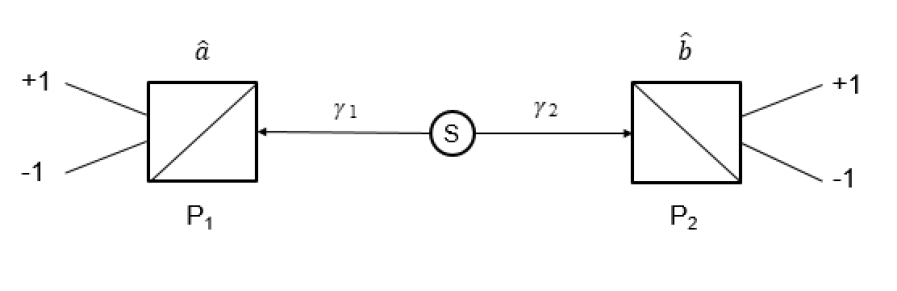
Figure 2: Schematic depiction of the experimental apparatus for measuring the polarization coefficient $E\left(\hat{a}\text{, }\hat{b}\right)$ in the Aspect-Grangier-Roger (AGR) experiment in Ref. aspect82 . Two photons $\gamma_{1}$ and $\gamma_{2}$ generated by a source $\mathrm{S}$ are in a singlet state $\left|\psi\right\rangle$ and propagate in opposite directions. The linear polarizations $\left(\pm 1\right)$ of $\gamma_{1}$ and $\gamma_{2}$ are measured along the orientations $\hat{a}$ and $\hat{b}$ specifying a pair of two-channel polarizers $\mathrm{P}_{\mathrm{1}}$ and $\mathrm{P}_{\mathrm{2}}$. The polarization coefficient $E\left(\hat{a}\text{, }\hat{b}\right)$ is experimentally determined by measuring, in a single run, the four coincidence counting rates $R_{\pm\pm}\left(\hat{a}\text{, }\hat{b}\right)$.

V.2 The 1982 AGR experiment

In Ref. aspect82 , Aspect and collaborators proposed the first experimental realization of the EPR gedankenexperiment. In this experiment, they used the optical analogs of the Stern-Gerlach filters (i.e., two-channel polarizers) to measure the linear-polarization correlation of pairs of photons emitted in a radiative cascade of calcium. Specifically, considering that the quantity $S_{\mathrm{RLHVT}}$ $\in\left[-2\text{, }2\right]$ given within a RLHVT by

$$S_{\mathrm{RLHVT}}=E(\hat{a},\hat{b})-E(\hat{a},\hat{b}^{\prime})+E(\hat{a}^{\prime},\hat{b})+E(\hat{a}^{\prime},\hat{b}^{\prime})\text{,}$$ (54)

Aspect and collaborators found $S_{\mathrm{\exp}}=2.697\pm 0.015$ for their chosen set of orientations $\left\{\hat{a}\text{, }\hat{b}\text{, }\hat{a}^{\prime}\text{, }\hat{b}^{\prime}\right\}$. They compared $S_{\mathrm{\exp}}$ with $S_{\mathrm{QM}}=2.70\pm 0.05$ predicted by QM. They concluded that their experimental findings were in excellent agreement with quantum-mechanical predictions and, thus, Bell’s inequality was significantly violated. For completeness, we point out that the correlation coefficient $E(\hat{a}$, $\hat{b})$ can be expressed, from an experimental standpoint, as

$$E(\hat{a}\text{, }\hat{b})\overset{\text{def}}{=}P_{++}(\hat{a}\text{, }\hat{b})+P_{--}(\hat{a}\text{, }\hat{b})-P_{+-}(\hat{a}\text{, }\hat{b})-P_{-+}(\hat{a}\text{, }\hat{b})\text{,}$$ (55)

where the probabilities $P_{ij}(\hat{a}$, $\hat{b})$ with $i$, $j\in\left\{+\text{, }-\right\}$ are defined as

$$P_{ij}(\hat{a}\text{, }\hat{b})\overset{\text{def}}{=}\frac{R_{ij}(\hat{a}\text{, }\hat{b})}{R_{ii}(\hat{a}\text{, }\hat{b})+R_{jj}(\hat{a}\text{, }\hat{b})+R_{ij}(\hat{a}\text{, }\hat{b})+R_{ji}(\hat{a}\text{, }\hat{b})}\text{.}$$ (56)

Given that a measurement along $\hat{a}$ yields the result $+1$ ($-1$) if the polarization of the photon is found parallel (perpendicular) to $\hat{a}$, $P_{\pm\pm}(\hat{a}$, $\hat{b})$ in Eq. (55) denote the probabilities of measuring outcomes $\pm 1$ along $\hat{a}$ for particle-$1$ and $\pm 1$ along $\hat{b}$ for particle-$2$. Moreover, $R_{\pm\pm}(\hat{a}$, $\hat{b})$ in Eq. (56) denote the coincidence counting rates of measuring outcomes $\pm 1$ along $\hat{a}$ for particle-$1$ and $\pm 1$ along $\hat{b}$ for particle-$2$.

V.3 From RLHVT and QM to experiment

In Fig. $2$, we depict the experimental apparatus for measuring the polarization coefficient (i.e., $E_{\mathrm{RLHVT}}(\hat{a}$, $\hat{b})$ in Eq. (7)) in the Aspect-Grangier-Roger (AGR) experiment. We are now in a good position to outline the logical steps connecting theoretical predictions that emerge from a realistic logical hidden variable theory (RLHVT) and quantum mechanics (QM) bell64 ; clauser69 ; bell04 to experimental observations in the Aspect-Grangier-Roger experiment aspect82 . First, the Bell inequality is initially expressed in terms of $E_{\mathrm{RLHVT}}(\hat{a}$, $\hat{b})$-like coefficients with $E_{\mathrm{RLHVT}}(\hat{a}$, $\hat{b})\overset{\text{def}}{=}\int\bar{A}\left(\hat{a}\text{, }\lambda\right)\bar{B}(\hat{b}$, $\lambda)\rho\left(\lambda\right)d\lambda$ in Eq. (7). Second, identifying $E_{{}_{\mathrm{QM}}}(\hat{a}$, $\hat{b})\overset{\text{def}}{=}\left\langle\psi|\left(\vec{\sigma}\cdot\hat{a}\right)\otimes(\vec{\sigma}\cdot\hat{b})|\psi\right\rangle$ with $E_{\mathrm{RLHVT}}(\hat{a}$, $\hat{b})$, the Bell inequality can be recast in terms of $E_{{}_{\mathrm{QM}}}(\hat{a}$, $\hat{b})$-like coefficients. Third, one shows that for any entangled quantum state $\left|\psi\right\rangle$ with $\left\langle\psi|\psi\right\rangle=1$, the Bell inequality in terms of $E_{{}_{\mathrm{QM}}}(\hat{a}$, $\hat{b})$-like coefficients can be violated gisin91 . Finally, it can be verified that quantum mechanical predictions, unlike theoretical predictions arising from a realistic logical hidden variable theory, agree with experimental observations expressed in terms of $E_{\mathrm{AGR}\text{-{exp}}}(\hat{a}$, $\hat{b})$, where aspect82

$$E_{\mathrm{AGR}\text{-{exp}}}(\hat{a}\text{, }\hat{b})\overset{\text{def}}{=}\frac{R_{++}(\hat{a}\text{, }\hat{b})+R_{--}(\hat{a}\text{, }\hat{b})-R_{+-}(\hat{a}\text{, }\hat{b})-R_{-+}(\hat{a}\text{, }\hat{b})}{R_{++}(\hat{a}\text{, }\hat{b})+R_{--}(\hat{a}\text{, }\hat{b})+R_{+-}(\hat{a}\text{, }\hat{b})+R_{-+}(\hat{a}\text{, }\hat{b})}\text{.}$$ (57)

These logical steps can be outlined as follows:

1. Derive the Bell inequality in the Clause-Horne-Shimony-Holt (CHSH) form within the formalism of a realistic logical hidden variable theory (RLHVT),

   $$\left|E_{\mathrm{RLHVT}}(\hat{a}\text{, }\hat{b})-E_{\mathrm{RLHVT}}(\hat{a}\text{, }\hat{b}^{\prime})\right|+\left|E_{\mathrm{RLHVT}}(\hat{a}^{\prime}\text{, }\hat{b})+E_{\mathrm{RLHVT}}(\hat{a}^{\prime}\text{, }\hat{b}^{\prime})\right|\leq 2\text{.}$$ (58)

2. Identify $P(\hat{a}$, $\hat{b})\overset{\text{def}}{=}E_{{}_{\mathrm{QM}}}(\hat{a}$, $\hat{b})$ with $E_{\mathrm{RLHVT}}(\hat{a}$, $\hat{b})$. Note that $P(\hat{a}$, $\hat{b})$ and $P\left(a\text{, }b\right)$ in the main text denote the same quantity.

3. Rewrite the Bell inequality in [i] by using the identification in [ii],

   $$\left|P(\hat{a}\text{, }\hat{b})-(P\hat{a}\text{, }\hat{b}^{\prime})\right|+\left|P(\hat{a}^{\prime}\text{, }\hat{b})+P(\hat{a}^{\prime}\text{, }\hat{b}^{\prime})\right|\leq 2\text{.}$$ (59)

4. Show that there are quantum mechanical states $\left|\psi\right\rangle$ (i.e., entangled states) for which the Bell inequality in Eq. (59) is violated. For instance,

   $$\left|P(\hat{a}\text{, }\hat{b})-P(\hat{a}\text{, }\hat{b}^{\prime})\right|+\left|P(\hat{a}^{\prime}\text{, }\hat{b})+P(\hat{a}^{\prime}\text{, }\hat{b}^{\prime})\right|>2\text{.}$$ (60)

   In particular, for a given entangled state $\left|\psi\right\rangle$, the strength of the violation depends on the sets of orientations $(\hat{a}$, $\hat{b})$, $(\hat{a}$, $\hat{b}^{\prime})$, $(\hat{a}^{\prime}$, $\hat{b})$, and $(\hat{a}^{\prime}$, $\hat{b}^{\prime})$.

5. Confirm, by means of the Aspect-Grangier-Roger experiment aspect82 , the violation of the Bell inequality in the CHSH form once $E_{\mathrm{AGR}\text{-{exp}}}(\hat{a}$, $\hat{b})$ in Eq. (57) is identified with $E_{{}_{\mathrm{QM}}}(\hat{a}$, $\hat{b})$.

In Table III, we report the expressions of spin correlation coefficients in a realistic local hidden variable theory (RLHVT), in quantum mechanics (QM) and, finally, in the Aspect-Grangier-Roger experiment (AGR-exp).

Theory and experiment	Spin correlation coefficient symbol	Spin correlation coefficient expression
Realistic local hidden variable theory	$E_{\mathrm{RLHVT}}\left(\hat{a}\text{, }\hat{b}\right)$	$\int\bar{A}\left(\hat{a}\text{, }\lambda\right)\bar{B}\left(\hat{b}\text{, }\lambda\right)\rho\left(\lambda\right)d\lambda$
Quantum mechanics	$E_{\mathrm{QM}}\left(\hat{a}\text{, }\hat{b}\right)$	$\left\langle\psi|\left(\vec{\sigma}\cdot\hat{a}\right)\otimes\left(\vec{\sigma}\cdot\hat{b}\right)|\psi\right\rangle$
The Aspect-Grangier-Roger experiment	$E_{\mathrm{AGR}\text{-{exp}}}\left(\hat{a}\text{, }\hat{b}\right)$	$\frac{R_{++}\left(\hat{a}\text{, }\hat{b}\right)+R_{--}\left(\hat{a}\text{, }\hat{b}\right)-R_{+-}\left(\hat{a}\text{, }\hat{b}\right)-R_{-+}\left(\hat{a}\text{, }\hat{b}\right)}{R_{++}\left(\hat{a}\text{, }\hat{b}\right)+R_{--}\left(\hat{a}\text{, }\hat{b}\right)+R_{+-}\left(\hat{a}\text{, }\hat{b}\right)+R_{-+}\left(\hat{a}\text{, }\hat{b}\right)}$

Table 5: Expressions of spin correlation coefficients in a realistic local hidden variable theory (RLHVT), in quantum mechanics (QM) and, finally, in the Aspect-Grangier-Roger experiment (AGR-exp).

VI Conclusions

In this paper, we presented a revisitation of the violation of Bell’s inequality in the CHSH form with entangled quantum states. First, we discussed the 1935 EPR paradox that emerges from putting the emphasis on Einstein’s locality and the absolute character of physical phenomena. Second, we discussed Bell’s 1971 derivation of the 1969 CHSH form of the original 1964 Bell inequality in the context of a RLHVT. Third, identifying the quantum-mechanical spin correlation coefficient with the RLHVT one, we followed Gisin’s 1991 analysis to show that QM violates Bell’s inequality when systems are in entangled quantum states. For pedagogical purposes, we showed how this violation depends both on the orientation of the polarizers and the degree of entanglement of the quantum states (see Fig. $1$, for instance). Fourth, we discussed the basics of the experimental verification of Bell’s inequality in an actual laboratory as presented in the original 1982 AGR) experiment.

In what follows, we present a summary of take home messages from our discussion on this beautiful piece of physical science with a deep interplay between theory (i.e., scientific imagination and theoretical creativity) and experiments (i.e., cleverly designed experimental set-ups and high statistical accuracy):

1. From the EPR paradox epr , one might intuitively think that the statistical predictions of quantum mechanics emerge from a hidden underlying deterministic substructure that encodes the natural assumption of locality.

2. John Bell derived Bell’s inequality within the framework of a realistic local-hidden variable theory bell64 ; bell04 .

3. Quantum mechanics is a non-local theory and violates Bell’s inequality bell64 ; bell04 .

4. Natural phenomena occur in a laboratory, not in a Hilbert space peres2004 . The experiments with entangled photons by Aspect and collaborators aspect82 ; aspect82B , Clauser and collaborators clauser69 ; clauser72 and, finally, Zeilinger and collaborators pan98 experimentally establish the violation of Bell’s inequalities and give evidence of one of the most striking aspects of quantum physics (i.e., quantum entanglement).

5. Entanglement is the key concept needed to understand the EPR paradox and the violation of Bell’s inequality by quantum mechanics pan98 ; zeilinger98 ; brukner01 .

6. Unlike what one might intuitively believe, quantum entanglement requires neither the entangled particles to come from a common source nor to have interacted in the past. This fact was experimentally verified by Zeilinger and collaborators in Ref. pan98 .

7. As pointed out by Zeiliger in Ref. zeilinger98 , information about quantum systems is more important than any possible so-called “real” property these systems might possess. Finally, there appears to exist no quantum world. Instead, as pointed out by Bohr in Ref. bohr35 , there is only an abstract quantum-mechanical description of natural phenomena.

This set of take home messages concludes our revisitation of the violation of Bell’s inequality in the Clauser-Horne-Shimony-Holt form with entangled quantum states. Interestingly, our idea of this revisitation started at the end of 2021 and, with our gladness, it is a very nice coincidence that the Nobel prize in Physics was assigned in 2022 to Aspect, Clauser, and Zeilinger epjd22 . Clearly, we express our congratulations to these three physicists along with their research Groups. Finally, we wholeheartedly believe this whole chain of events- EPR, Bohr, Bell, entanglement, interplay between theory and experiment- is the essence of physics at its best. We are aware that our effort here is in no way representative of this wonderful scientific endeavor. It would have been too big a task for us to accomplish in the present scientific effort. However, being this paper written by two theorists, a young undergraduate student, and an experimental physicist, we hope it will help young students and future generations of researchers appreciate (via a description of a sequence of actual scientific events) how important are the processes of scientific imagination and experimental verification in modern physics.

- (1) A. Peres and D. R. Terno, Quantum information and relativity theory, Rev. Mod. Phys. 76, 93 (2004).
- (2) C. Corda, Dark energy and dark matter like intrinsic curvature in extended gravity. Viability through gravitational waves, New Advances in Physics 7, 67 (2013).
- (3) L. D. Landau and E. M. Lifshitz, The Classical Theory of Fields, Pergamon Press Ltd. (1971).
- (4) C. Corda, Interferometric detection of gravitational waves: The definitive test for general relativity, Int. J. Mod. Phys. D18, 2275 (2009).
- (5) J. D. Bekenstein, Quantum black holes as atoms, in Proceedings of th Eight Marcel Grossmann Meeting, T. Piran and R. Ruffini, eds., pp. 92-111, World Scientific Singapore (1999).
- (6) A. Pais, Subtle Is the Lord: The Science and the Life of Albert Einstein, Oxford University Press (2005).
- (7) J. J. Sakurai, Modern Quantum Mechanics, The Benjamin/Cummings Publishing Company, Inc. (1985).
- (8) R. Colella, A. W. Overhauser, and S. A. Werner, Observation of gravitationally induced quantum interference, Phys. Rev. Lett. 34, 1472 (1975).
- (9) C. W. Misner, K. S. Thorne and J. A. Wheeler, Gravitation, W. H. Feeman and Company (1973).
- (10) C. Brukner, Quantum causality, Nature Physics 10, 259 (2014).
- (11) N. Bohr, Can quantum-mechanical description of physical reality be considered complete?, Phys. Rev. 48, 696 (1935).
- (12) N. Bohr, Causality and complementarity, Philosophy of Science 4, 289 (1937).
- (13) N. Bohr, On the notions of causality and complementarity, Science 111, 51 (1950).
- (14) J. A. Wheeler, No fugitive and cloistered virtue- A tribute to Niels Bohr, Physics Today 16, 30 (1963).
- (15) J. A. Vaccaro, Group theoretic formulation of complementarity, arXiv:quant-ph/1012.3532 (2010).
- (16) A. Einstein, B. Podolsky, and N. Rosen, Can quantum-mechanical description of physical reality be considered complete?, Phys. Rev. 47, 777 (1935).
- (17) R. Omnes, The Interpretation of Quantum Mechanics, Princeton University Press (1994).
- (18) D. Bohm, Quantum Theory, Prentice-Hall, Englewood Cliffs, New Jersey (1951).
- (19) D. Bohm and Y. Aharonov, Discussion of experimental proof for the paradox of Einstein, Rosen, and Podolsky, Phys. Rev. 108, 1070 (1957).
- (20) F. Laloe, Do we really understand quantum mechanics? Strange correlations, paradoxes, and theorems, Am. J. Phys. 69, 655 (2012).
- (21) A. Peres, Unperformed experiments have no results, Am. J. Phys. 46, 745 (1978).
- (22) S. W. Hawking, Breakdown of predictability in gravitational collapse, Phys. Rev. D14, 2460 (1976).
- (23) X. Calmet and S. D. H. Hsu, A brief history of Hawking’s information paradox, Eur. Phys. Lett. 139, 49001 (2022).
- (24) J. S. Bell, On the Einstein Podolsky Rosen paradox, Physics 1, 195 (1964).
- (25) N. Gisin, Bell’s inequality holds for all non-product states, Phys. Lett. A154, 201 (1991).
- (26) C. Cafaro, S. A. Ali, and A. Giffin, On the violation of Bell’s inequality for all non-product quantum states, Int. J. Quantum Inf. 14, 1630003 (2016).
- (27) Private communication between C. C. and Elena R. Loubenets and, later, between C. C. and Yanjun He.
- (28) J. F. Clauser, M. A. Horne, A. Shimony, and R. A. Holt, Proposed experiment to test local hidden variable theories, Phys. Rev. Lett. 23, 880 (1969).
- (29) A. Aspect, P. Grangier, and G. Roger, Experimental realization of Einstein-Podoslky-Rosen-Bohm Gedankenexperiment: A new violation of Bell’s inequalities, Phys. Rev. Lett. 49, 91 (1982).
- (30) A. Peres, Quantum Theory: Concepts and Methods, Kluwer Academic Publishers (1995).
- (31) A. Peres, Quantum information and general relativity, arXiv:quant-ph/0405127 (2004).
- (32) H. P. Stapp, Bell’s theorem and world process, Il Nuovo Cimento 29, 270 (1975).
- (33) J. S. Bell, Speakable and Unspeakable in Quantum Mechanics, Cambridge University Press (2004).
- (34) N. Gisin and A. Peres, Maximal violation of Bell’s inequality for arbitrary large spin, Phys. Lett. A162, 15 (1992).
- (35) P. Kaye, R. Laflamme, and M. Mosca, An Introduction to Quantum Computing, Oxford University Press (2007).
- (36) D. Collins, N. Gisin, N. Linden, S. Massar, and S. Popescu, Bell inequalities for arbitrarily high-dimensional systems, Phys. Rev. Lett. 88, 040404 (2002).
- (37) C. H. Bennett, H. J. Bernstein, S. Popescu and B. Schumacher, Concentrating partial entanglement by local operations, Phys. Rev. A53, 2046 (1996).
- (38) J. Leach, B. Jack, J. Romero, M. Ritsch-Marte, R. W. Boyd, A. K. Jha, S. M. Barnett, S. Franke-Arnold and M. J. Padgett, Violation of a Bell inequality in two-dimensional orbital angular momentum state-spaces, Opt. Express 17, 8287 (2009).
- (39) J. Dunningham and V. Vedral, Introductory Quantum Physics and Relativity, Imperial College Press (2011).
- (40) M. A. Nielsen and I. L. Chuang, Quantum Computation and Quantum Information, Cambridge University Press (2000).
- (41) C. Cafaro and S. Mancini, Characterizing the depolarizing quantum channel in terms of Riemannian geometry, Int. J. Geom. Methods Mod. Phys. 9, 1260020 (2012).
- (42) C. Cafaro and S. Mancini, Quantum stabilizer codes for correlated and asymmetric depolarizing errors, Phys. Rev. A82, 012306 (2010).
- (43) C. Cafaro and P. van Loock, Approximate quantum error correction for generalized amplitude-damping errors, Phys. Rev. A89, 022316 (2014).
- (44) C. Cafaro, S. Ray, and P. M. Alsing, Optimal-speed unitary quantum time evolutions and propagation of light with maximal degree of coherence, Phys. Rev. A105, 052425 (2022).
- (45) N. Brunner, D. Cavalcanti, S. Pironio, V. Scarani, and S. Wehner, Bell nonlocality, Rev. Mod. Phys. 86, 419 (2014).
- (46) C. S. Wu and I. Shaknov, The angular correlation of scattered annihilation radiation, Phys. Rev. 77, 136 (1950).
- (47) C. A. Kocher and E. D. Commins, Polarization correlation of photons emitted in an atomic cascade, Phys. Rev. Lett. 18, 575 (1967).
- (48) S. J. Freedman and J. F. Clauser, Experimental test of local hidden-variable theories, Phys. Rev. Lett. 28, 938 (1972).
- (49) A. Aspect, P. Grangier, and G. Roger, Experimental tests of realistic local theories via Bell’s theorem, Phys. Rev. Lett. 47, 460 (1981).
- (50) A. Aspect, J. Dalibard, and G. Roger, Experimental test of Bell’s inequalities using time-varying analyzers, Phys. Rev. Lett. 49, 1804 (1982).
- (51) G. Weihs, T. Jennewein, C. Simon, H. Weinfurter, and A. Zeilinger, Violation of Bell’s inequality under strict Einstein locality conditions, Phys. Rev. Lett. 81, 5039 (1998).
- (52) A. Aspect, Bell’s inequality test: More ideal than ever, Nature 398, 189 (1999).
- (53) B. Hensen et al., Loophole-free Bell inequality violation using electron spins separated by 1.3 kilometres, Nature 526, 682 (2015).
- (54) J.-Å. Larsson, Loopholes in Bell inequality tests of local realism, J. Phys. A: Math. Theor. 47, 424003 (2014).
- (55) J.-W. Pan, D. Bouwmeester, H. Weinfurter, and A. Zeilinger, Experimental entanglement swapping: Entangling photons that never interacted, Phys. Rev. Lett. 80, 3891 (1998).
- (56) A. Zeilinger, Quantum entanglement: A fundamental concept finding its applications, Phys. Scr. T76, 203 (1998).
- (57) C. Brukner, M. Zukowski, and A. Zeilinger, The essence of entanglement, in Quantum Arrangements, Fundamental Theories of Physics Book Series, Springer, vol. 203, pp. 117-138 (2021).
- (58) W. D. Phillips and J. Dalibard, Experimental tests of Bell’s inequalities: A first-hand account by Alain Aspect, Eur. Phys. J. D77, 8 (2022).