The SLE Bubble Measure via Conformal Welding of Quantum Surfaces

Abstract.

We showed that the $\mathrm{SLE}_{\kappa}(\rho)$ bubble measure recently constructed by Zhan arises naturally from the conformal welding of two Liouville quantum gravity (LQG) disks. The proof relies on (1) a “quantum version” of the limiting construction of the SLE bubble, (2) the conformal welding between quantum triangles and quantum disks due to Ang, Sun and Yu, and (3) the uniform embedding techniques of Ang, Holden and Sun. As a by-product of our proof, we obtained a decomposition formula of the $\mathrm{SLE}_{\kappa}(\rho)$ bubble measure. Furthermore, we provided two applications of our conformal welding results. First, we computed the moments of the conformal radius of the $\mathrm{SLE}_{\kappa}(\rho)$ bubble on $\mathbb{H}$ conditioning on surrounding $i$. The second application concerns the bulk-boundary correlation function in the Liouville Conformal Field Theory (LCFT). Within probabilistic frameworks, we derived a formula linking the bulk-boundary correlation function in the LCFT to the joint law of left & right quantum boundary lengths and the quantum area of the two-pointed quantum disk. This relation is used by Ang, Remy, Sun and Zhu in a concurrent work to verify the formula of two-pointed bulk-boundary correlation function in physics predicted by Hosomichi (2001).

1. Introduction

The Schramm-Loewner evolution ($\mathrm{SLE}$) and Liouville quantum gravity (LQG) are central objects in Random Conformal Geometry and it was shown in [She10] and [DMS20] that SLE curves arise naturally as the interfaces of LQG surfaces under conformal welding. Conformal welding results in [She10, DMS20] mainly focus on the infinite volume LQG surfaces. Recently, Ang, Holden and Sun [AHS20] showed that conformal welding of finite-volume quantum surfaces called two-pointed quantum disks can give rise to canonical variants of $\mathrm{SLE}$ curves with two marked points. Later, it was shown by Ang, Holden and Sun [AHS22] that another canonical invariant of $\mathrm{SLE}$ called $\mathrm{SLE}$ Loop is the natural welding interface of two quantum disks without marked points. The resulting LQG surface is called the quantum sphere, which describes the scaling limit of classical planar map models with spherical topology.

As will be reviewed in Section 2.2, the rooted $\mathrm{SLE}_{\kappa}(\rho)$ bubble measure on $\mathbb{H}$ is an important one parameter family of random Jordan curves constructed by Zhan [Zha22] for all $\kappa>0$ and $\rho>-2$. When $\kappa>4$ and $\rho\in(-2,\frac{\kappa}{2}-4]$, the law of the bubble is a probability measure and satisfies conformal invariance property ([Zha22, Theorem 3.10]). When $\rho>(-2)\vee(\frac{\kappa}{2}-4)$, the law of the bubble is a $\sigma$-finite infinite measure and satisfies conformal covariance property ([Zha22, Theorem 3.16]). In both cases, an instance $\eta$ of $\mathrm{SLE}_{\kappa}(\rho)$ bubble is characterized by the following Domain Markov Property (DMP): suppose $\tau$ is a positive stopping time for $\eta$, then conditioning on $\eta[0,\tau]$ and the event that $\eta$ is not completed at $\tau$, the rest of $\eta$ is a chordal $\mathrm{SLE}_{\kappa}(\rho)$ on $\mathbb{H}\backslash\eta[0,\tau]$ ([Zha22, Theorem 3.16]). Moreover, it was shown that $\mathrm{SLE}_{\kappa}(\rho)$ bubble measure can be viewed as the weak limit of chordal $\mathrm{SLE}_{\kappa}(\rho)$ on $\mathbb{H}$ from $0$ to $\varepsilon$ as $\varepsilon\to 0^{+}$ (with force point at $0^{-}$) after suitable rescaling ([Zha22, Theorem 3.20]).

On the other hand, it was shown in [ARS22, Section 4] that a particular $\mathrm{SLE}_{\kappa}(\rho)$ bubble curve can be obtained from conformally welding two Liouville quantum gravity surfaces of the disk topology. This was used to derive the Fateev-Zamolodchikov-Zamolodchikov (FZZ) formula in Liouville theory, which serves as a crucial input to the proof of the imaginary DOZZ formula for conformal loop ensemble (CLE) on the Riemann sphere [AS21]. This paper generalizes the conformal welding result in [ARS22] to all $\rho>-2$; see Remark 1.2 for the precise relation between our result and the one in [ARS22].

The rest of the paper is organized as follows. We state our main conformal welding results, including Theorem 1.1 and Theorem 1.3, in Section 1.1 and Theorem 1.5 with its applications in Section 1.2. All the necessary backgrounds on Random Conformal Geometry will be reviewed in Section 2. We first prove Theorem 1.1 in Sections 3 and 4 and then prove Theorem 1.3 in Section 5 based on Theorem 1.1 and the uniform embedding of LQG surfaces. Next, we prove Theorem 1.5, which is the generalization of Theorem 1.1 to the case when the bulk insertion of the quantum surface has generic weight. In Section 7, we discuss two applications of Theorem 1.5: The first application concerns the computation of the moments of the conformal radius of the $\mathrm{SLE}_{\kappa}(\rho)$ bubble on $\mathbb{H}$ conditioning on surrounding $i$; Secondly, we derive a formula linking the bulk-boundary correlation function in LCFT to the joint law of left & right quantum boundary lengths and the quantum area of the two-pointed quantum disk. Finally, in Section 8, we will discuss several conjectures that arise naturally from the contexts of this paper, including a generalization of the $\mathrm{SLE}_{\kappa}(\rho)$ bubble and the scaling limit of bubble-decorated disk quadrangulations.

1.1. $\mathrm{SLE}_{\kappa}(\rho)$ bubble measures via conformal welding of quantum disks

Let $\mathrm{Bubble}_{\mathbb{H}}(p)$ be the space of rooted simple loops on $\mathbb{H}$ with root $p\in\mathbb{R}$. Precisely, an oriented simple closed loop $\eta$ is in $\mathrm{Bubble}_{\mathbb{H}}(p)$ if and only if $p\in\eta,(\eta\backslash\{p\})\subseteq\overline{\mathbb{H}}$. Throughout this paper, for $\eta\in\mathrm{Bubble}_{\mathbb{H}}(p)$, let $D_{\eta}(p)$ be the connected component of $\mathbb{H}\backslash\eta$ which is encircled by $\eta$ and let $D_{\eta}(\infty)$ be the domain $\mathbb{H}\backslash(\eta\cup D_{\eta}(p))$ containing $\infty$. The point $p$ corresponds to two pseudo boundary marked points $p^{-}$ and $p^{+}$ on $D_{\eta}(\infty)$. Let $\mathrm{SLE}_{\kappa,0}^{\mathrm{bubble}}(\rho)$ denote the rooted $\mathrm{SLE}_{\kappa}(\rho)$ bubble measure with root $0$ studied in [Zha22] (see Definition 2.3) and this is a $\sigma$-finite infinite measure on the space $\mathrm{Bubble}_{\mathbb{H}}(0)$.

For each $\gamma\in(0,2)$, there is a family of LQG surfaces with disk topology called quantum disks. There is also a weight parameter $W>0$ associated with the family of quantum disks. Let $\mathcal{M}^{\mathrm{disk}}_{0,2}(W)$ denote the two-pointed weight-$W$ quantum disk; both marked points are on the boundary, each with weight $W$ (see Definition 2.15 and 2.19 for two regimes in terms of $W$). When $W=2$, the two marked points in quantum disk $\mathcal{M}_{0,2}^{\mathrm{disk}}(2)$ are quantum typical w.r.t. the quantum boundary length measure ([AHS20, Proposition $A.8$]) and we denote the $\mathcal{M}_{0,2}^{\mathrm{disk}}(2)$ by $\mathrm{QD}_{0,2}$. Let $\mathrm{QD}_{0,1}$ and $\mathrm{QD}_{1,1}$ denote the typical quantum disks with one boundary marked point and with one bulk $\&$ one boundary marked point respectively (see Definition 2.21 for the class of typical quantum disks and its variants).

Let $\mathrm{QD}_{0,1}(\ell)$ and $\mathrm{QD}_{1,1}(\ell)$ be the disintegration of $\mathrm{QD}_{0,1}$ and $\mathrm{QD}_{1,1}$ over its quantum boundary length respectively, i.e., $\mathrm{QD}_{0,1}=\int_{0}^{\infty}\mathrm{QD}_{0,1}(\ell)d\ell$ and $\mathrm{QD}_{1,1}=\int_{0}^{\infty}\mathrm{QD}_{1,1}(\ell)d\ell$, and both $\mathrm{QD}_{0,1}(\ell)$ and $\mathrm{QD}_{1,1}(\ell)$ should be understood as $\mathrm{QD}_{0,1}$ and $\mathrm{QD}_{1,1}$ restricted to having total boundary length $\ell$ respectively. Similarly, let $\mathcal{M}^{\mathrm{disk}}_{0,2}(W;\cdot,\ell)$ be the disintegration of $\mathcal{M}^{\mathrm{disk}}_{0,2}(W)$ over its right boundary, i.e., $\mathcal{M}^{\mathrm{disk}}_{0,2}(W)=\int_{0}^{\infty}\mathcal{M}^{\mathrm{disk}}_{0,2}(W;\cdot,\ell)d\ell$, and the $\mathcal{M}^{\mathrm{disk}}_{0,2}(W;\cdot,\ell)$ again represents the $\mathcal{M}^{\mathrm{disk}}_{0,2}(W)$ restricted to having the right boundary length $\ell$. Let $\int_{0}^{\infty}\mathcal{M}^{\mathrm{disk}}_{0,2}(W;\cdot,\ell)\times\mathrm{QD}_{0,1}(\ell)d\ell$ be the curve-decorated quantum surface obtained by conformally welding the right boundary of $\mathcal{M}^{\mathrm{disk}}_{0,2}(W)$ and total boundary of $\mathrm{QD}_{0,1}$. Similarly, $\int_{0}^{\infty}\mathcal{M}^{\mathrm{disk}}_{0,2}(W;\cdot,\ell)\times\mathrm{QD}_{1,1}(\ell)d\ell$ is the quantum surface obtained by welding the right boundary of $\mathcal{M}^{\mathrm{disk}}_{0,2}(W)$ and the total boundary of $\mathrm{QD}_{1,1}$.

In theoretical physics, LQG originated in A. Polyakov’s seminal work [Pol81] where he proposed a theory of summation over the space of Riemannian metrics on fixed two dimensional surface. The fundamental building block of his framework is the Liouville conformal field theory (LCFT), which describes the law of the conformal factor of the metric tensor in a surface of fixed complex structure. The LCFT was made rigorous in probability theory in various different topologies; see [DKRV16] and [HRV18] for the case of Riemann sphere and of simply connected domain with boundary respectively, and [DRV15, Rem17, GRV19] for the case of other topologies.

To be precise, let $P_{\mathbb{H}}$ be the probability measure corresponding to the law of the free-boundary Gaussian free field (GFF) on $\mathbb{H}$ normalized to having average zero on the unit circle in upper half plane unit circle $\partial\mathbb{D}\cap\mathbb{H}$. The infinite measure $\mathrm{LF}_{\mathbb{H}}(d\phi)$ is defined by first sampling $(h,\mathbf{c})$ according to $P_{\mathbb{H}}\times\left[e^{-Qc}dc\right]$ and then letting $\phi(z)=h(z)-2Q\log|z|_{+}+\mathbf{c}$, where $Q=\frac{2}{\gamma}+\frac{\gamma}{2}$ and $|z|_{+}=\max\{|z|,1\}$. We can further define the Liouville field with bulk or/and boundary insertion(s), e.g., $\mathrm{LF}_{\mathbb{H}}^{(\beta,p)}$ and $\mathrm{LF}_{\mathbb{H}}^{(\alpha,z),(\beta,p)}$, where $p\in\mathbb{R}$ and $z\in\mathbb{H}$. To make sense of $\mathrm{LF}_{\mathbb{H}}^{(\beta,p)}$, where $p\in\partial\mathbb{H}$, let $\mathrm{LF}_{\mathbb{H}}^{(\beta,p)}:=\lim_{\varepsilon\to 0}\varepsilon^{\beta^{2}/4}e^{\frac{\beta}{2}\phi_{\varepsilon}(p)}\mathrm{LF}_{\mathbb{H}}(d\phi)$, $\phi_{\varepsilon}$ being a suitable regularization at scale $\varepsilon$ of $\phi$. In terms of $\mathrm{LF}_{\mathbb{H}}^{(\alpha,z),(\beta,p)}$ with $z\in\mathbb{H}$ and $p\in\partial\mathbb{H}$, we use the similar limiting procedure. Let $\mathrm{LF}_{\mathbb{H}}^{(\beta,p),(\alpha,z)}:=\lim_{\varepsilon\to 0}\varepsilon^{\alpha^{2}/2}e^{\alpha\phi_{\varepsilon}(z)}\mathrm{LF}_{\mathbb{H}}^{(\beta,p)}(d\phi)$, $\phi_{\varepsilon}(z)$ being some suitable renormalization at scale $\varepsilon$. By Cameron-Martin shift (a.k.a. Girsanov’s theorem), the $\mathrm{LF}_{\mathbb{H}}^{(\beta,p)}$ represents a sample from $\mathrm{LF}_{\mathbb{H}}$ plus a $\beta$-$\log$ singularity at boundary marked point $p$ locally. Similarly, $\mathrm{LF}_{\mathbb{H}}^{(\alpha,z),(\beta,p)}$ should be viewed as $\mathrm{LF}_{\mathbb{H}}$ plus one boundary $\beta$-$\log$ singularity at $p$ and one bulk $\alpha$-$\log$ singularity at $z$.

For $q\in\mathbb{H}$ and $p\in\partial\mathbb{H}$, let $\mathrm{Bubble}_{\mathbb{H}}(p,q)$ be the space of rooted simple loops on $\mathbb{H}$ rooted at $p$ and surrounding $q$. Precisely, an oriented simple closed loop $\eta$ is in $\mathrm{Bubble}_{\mathbb{H}}(p,q)$ if and only if $p\in\eta,(\eta\backslash\{p\})\subseteq\overline{\mathbb{H}}$ and $q\in D_{\eta}(p)$. Let $\mathrm{SLE}_{\kappa,0}^{\mathrm{bubble}}(\rho)[d\eta|{i\in D_{\eta}(0)}]$ denote the conditional law of $\mathrm{SLE}_{\kappa,0}^{\mathrm{bubble}}(\rho)$ on surrounding $i$ and this is a probability measure on $\mathrm{Bubble}_{\mathbb{H}}(0,i)$.

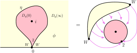
Figure 1. Illustration of Theorem 1.1 when $W\geq\frac{\gamma^{2}}{2}$: suppose $(\phi,\eta)$ is sampled from $C\cdot\mathrm{LF}_{\mathbb{H}}^{(\gamma,i),\beta_{2W+2},0)}(d\phi)\times\mathrm{SLE}_{\kappa,0}^{\mathrm{bubble}}(\rho)[d\eta|{i\in D_{\eta}(0)}]$ as shown on the left above, then the law of $(D_{\eta}(0),\phi,i,0)$ and $(D_{\eta}(\infty),\phi,0^{-},0^{+})$ viewed as a pair of marked quantum surfaces is equal to $\int_{0}^{\infty}\mathcal{M}^{\mathrm{disk}}_{0,2}(W;\cdot,\ell)\times\mathrm{QD}_{1,1}(\ell)d\ell$, i.e., the quantum surface obtained by conformally welding the total boundary of a sample from $\mathrm{QD}_{1,1}$ with the right boundary of a sample from $\mathcal{M}^{\mathrm{disk}}_{0,2}(W)$.

Theorem 1.1.

Fix $\gamma\in(0,2)$. For $W>0$, let $\rho=W-2$ and $\beta_{2W+2}=\gamma-\frac{2W}{\gamma}$. There exists some constant $C\in(0,\infty)$ such that suppose $(\phi,\eta)$ is sampled from

(1.1.1) $$C\cdot\mathrm{LF}_{\mathbb{H}}^{(\gamma,i),(\beta_{2W+2},0)}(d\phi)\times\mathrm{SLE}_{\kappa,0}^{\mathrm{bubble}}(\rho)[d\eta|{i\in D_{\eta}(0)}],$$

then the law of $(D_{\eta}(0),\phi,i,0)$ and $(D_{\eta}(\infty),\phi,0^{-},0^{+})$ viewed as a pair of marked quantum surfaces is equal to

(1.1.2) $$\int_{0}^{\infty}\mathcal{M}^{\mathrm{disk}}_{0,2}(W;\cdot,\ell)\times\mathrm{QD}_{1,1}(\ell)d\ell.$$

Remark 1.2.

In [ARS22], the authors considered the same type of conformal welding with $W=\frac{\gamma^{2}}{2}-2$ ([ARS22, Theorem 4.1]). This particular conformal welding result was used to obtained the so-called FZZ formula proposed in [FZZ00]. However in [ARS22, Theorem 4.1], the law of the welding interface was not explicitly specified. Here in the above Theorem 1.1, we generalized the [ARS22, Theorem 4.1] to all $W>0$, and furthermore identified the law of the welding interface to be the $\mathrm{SLE}_{\kappa}(W-2)$ bubble constructed in [Zha22].

The proof of Theorem 1.1 is separated into two parts. In Section 3, we show that the law of welding interface of curve-decorated quantum surface (1.1.2) is the $\mathrm{SLE}_{\kappa,0}^{\mathrm{bubble}}(\rho)$ conditioning on surrounding $i$ and moreover, it is independent of the underlying random field. To identify the law of the welding interface, we essentially use the “quantum version” of the limiting construction of the $\mathrm{SLE}_{\kappa}(\rho)$ bubble; see Corollary 2.4 for the statement on the Euclidean case. More precisely, we first consider the conformal welding of $\mathcal{M}^{\mathrm{disk}}_{0,2}(W)$ and $\mathrm{QD}_{1,2}$, i.e., the typical quantum disk with two boundary and one bulk marked points, whose welding interface is the chordal $\mathrm{SLE}_{\kappa}(\rho)$ conditioning on passing to the left of some fixed point in $\mathbb{H}$ (Lemma 3.5). Then conditioning on the quantum boundary length of $\mathrm{QD}_{1,2}$ between two boundary marked points shrinks to zero, we can construct a coupling with (1.1.2). Under such coupling, these two welding interfaces will match with high probability (Lemma 3.6). The independence of curve with the underlying random field follows from the coupling argument and Corollary 2.4 on the deterministic convergence of chordal $\mathrm{SLE}_{\kappa}(\rho)$.

The proof of the law of the underlying random field after conformal welding of two quantum disks, i.e., the quantum surface (1.1.2), is done in two steps. In Section 4, we first consider (1.1.2) when $0<W<\frac{\gamma^{2}}{2}$, i.e., when the two-pointed disk is thin. By Lemma 4.12, the thin quantum disk of weight $W$ with one additional typical boundary marked point can be viewed as the concatenation of three independent disks: two thin disks of weight $W$ and one thick disk of weight $\gamma^{2}-W$ with one typical boundary marked point. Therefore, we can first sample one typical boundary marked point on $\mathcal{M}^{\mathrm{disk}}_{0,2}(W)$ and then sample two typical boundary marked points on $\mathrm{QD}_{1,1}(\gamma,\alpha)$, i.e., the quantum disk with one generic boundary insertion (Definition 4.9). The field law after conformally welding $\mathcal{M}^{\mathrm{disk}}_{2,\bullet}(W)$ and $\mathrm{QD}_{1,3}(\gamma,\alpha)$ can be derived from conformal welding results for quantum triangles in [ASY22]. After de-weighting all the additional marked points, we solve the case when $0<W<\frac{\gamma^{2}}{2}$. To extend to the full range $W>0$, we inductively weld thin disks outside $\mathrm{QD}_{1,1}(\gamma,\alpha)$. By Theorem 2.22, a thick disk can be obtained by welding multiple thin disks. This concludes the outline of the proof of Theorem 1.1.

Next, we use the techniques of uniform embedding of quantum surfaces from [AHS21] to remove the bulk insertion in Theorem 1.1 so that the welding interface is the $\mathrm{SLE}_{\kappa}(\rho)$ bubble without conditioning. In order to introduce Theorem 1.3, we quickly recall the setups of the uniform embedding of upper half plane $\mathbb{H}$. Let $\mathrm{conf}(\mathbb{H})$ be the group of conformal automorphisms of $\mathbb{H}$ where the group multiplication $\cdot$ is the function composition $f\cdot g=f\circ g$. Let $\mathbf{m}_{\mathbb{H}}$ be a Haar measure on $\mathrm{conf}(\mathbb{H})$, which is both left and right invariant. Suppose $\mathfrak{f}$ is sampled from $\mathbf{m}_{\mathbb{H}}$ and $\phi\in C^{\infty}_{0}(\mathbb{H})^{\prime}$, i.e., $\phi$ is a generalized function, then we call the random function

(1.1.3) $$\mathfrak{f}\bullet_{\gamma}\phi=\phi\circ\mathfrak{f}^{-1}+Q|\log(\mathfrak{f}^{-1})^{\prime}|$$

the uniform embedding of $(\mathbb{H},\phi)$ via $\mathbf{m}_{\mathbb{H}}$. By invariance property of Haar measure, the law of $\mathfrak{f}\bullet_{\gamma}\phi$ only depends on $(\mathbb{H},\phi)$ as quantum surface. We write $\mathbf{m}_{\mathbb{H}}\ltimes\left(\int_{0}^{\infty}\mathcal{M}^{\mathrm{disk}}_{0,2}(W;\cdot,\ell)\times\mathrm{QD}_{0,1}(\ell)d\ell\right)$ as the law of $(\mathfrak{f}\bullet_{\gamma}h,f(\eta),f(r))$, where $(\mathbb{H},h,\eta,r)$ is an embedding of a sample from curve-decorated quantum surface $\int_{0}^{\infty}\mathcal{M}^{\mathrm{disk}}_{0,2}(W;\cdot,\ell)\times\mathrm{QD}_{0,1}(\ell)d\ell$, and $\mathfrak{f}$ is sampled independently from $\mathbf{m}_{\mathbb{H}}$. Notice that here the $\mathbf{m}_{\mathbb{H}}$ does not fix our boundary marked point $r$, which initially is the root of $\eta$.

The equation (1.1.3) also provides a natural equivalence relation $\sim_{\gamma}$ over curve-decorated quantum surfaces; two curve-decorated quantum surfaces $(D_{1},\phi_{1},\eta_{1},\omega_{1},\ldots,\omega_{n})$ with $\omega_{i}\in D_{1}\cup\partial D_{1}$ and $(D_{2},\phi_{2},\eta_{2},z_{1}\ldots,z_{n})$ with $z_{i}\in D_{2}\cup\partial D_{2}$ are equivalent as quantum surfaces, denoted by

(1.1.4) $$(D_{1},\phi_{1},\eta_{1},\omega_{1},\ldots,\omega_{n})\sim_{\gamma}(D_{2},\phi_{2},\eta_{2},z_{1}\ldots,z_{n}),$$

if there is a conformal map $\psi:D_{1}\to D_{2}$ such that $\phi_{2}=\psi\bullet_{\gamma}\phi_{1}$, $\eta_{2}=\psi(\eta_{1})$, and $\psi(\omega_{i})=z_{i},1\leq i\leq n$.

We can also consider the case when the marked points are fixed under the action of Haar measure. For fixed $p\in\partial\mathbb{H}$, let $\mathrm{conf}(\mathbb{H},p)$ be the subgroup of $\mathrm{conf}(\mathbb{H})$ fixing $p$ and let $\mathbf{m}_{\mathbb{H},p}$ be a Haar measure on $\mathrm{conf}(\mathbb{H},p)$. The curve-decorated quantum surface $\int_{0}^{\infty}\mathcal{M}^{\mathrm{disk}}_{0,2}(W;\cdot,\ell)\times\mathrm{QD}_{0,1}(\ell)d\ell$ can be identified as a measure on the product space $\left(C_{0}^{\infty}(\mathbb{H})^{\prime}/\mathrm{conf}(\mathbb{H},p)\right)\times\mathrm{Bubble}_{\mathbb{H}}(p)$. Therefore, the measure $\mathbf{m}_{\mathbb{H},p}\ltimes\left(\int_{0}^{\infty}\mathcal{M}^{\mathrm{disk}}_{0,2}(W;\cdot,\ell)\times\mathrm{QD}_{0,1}(\ell)d\ell\right)$ can be defined in the exact same way as $\mathbf{m}_{\mathbb{H}}\ltimes\left(\int_{0}^{\infty}\mathcal{M}^{\mathrm{disk}}_{0,2}(W;\cdot,\ell)\times\mathrm{QD}_{0,1}(\ell)d\ell\right)$ for fixed $p\in\partial\mathbb{H}$.

For any fixed $p\in\mathbb{H}$, let $\mathrm{SLE}_{\kappa,p}^{\mathrm{bubble}}(\rho)$ denote the $\mathrm{SLE}_{\kappa}(\rho)$ bubble measure rooted at $p\in\mathbb{R}$. It is easily defined as the image of $\mathrm{SLE}_{\kappa,0}^{\mathrm{bubble}}(\rho)$ under the shifting map $f_{p}:z\mapsto z+p$.

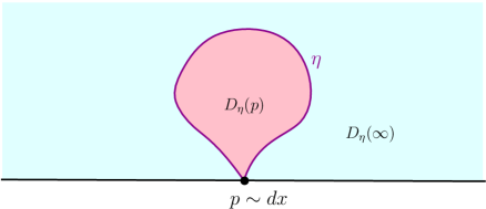
Figure 2. Illustration of the welding equation (1.1.5) in Theorem 1.3: first sample a root point $p$ according to Lebesgue measure $dx$ on $\mathbb{R}$, then sample $(\phi,\eta)$ according to the product measure $\mathrm{LF}^{(\beta_{2W+2},p)}_{\mathbb{H}}(d\phi)\times\mathrm{SLE}_{\kappa,p}^{\mathrm{bubble}}(W-2)(d\eta)$. The resulting quantum surface $(\mathbb{H},\phi,\eta,p)/\sim_{\gamma}$ has the law of $C\int_{0}^{\infty}\mathcal{M}^{\mathrm{disk}}_{0,2}(W;\cdot,\ell)\times\mathrm{QD}_{0,1}(\ell)d\ell$ after uniform embedding.

Theorem 1.3.

Fix $\gamma\in(0,2)$. For $W>0$, let $\rho=W-2$ and $\beta_{2W+2}=\gamma-\frac{2W}{\gamma}$. There exists some constant $C\in(0,\infty)$ such that

(1.1.5) $$\mathbf{m}_{\mathbb{H}}\ltimes\left(\int_{0}^{\infty}\mathcal{M}^{\mathrm{disk}}_{0,2}(W;\cdot,\ell)\times\mathrm{QD}_{0,1}(\ell)d\ell\right)=C\cdot\mathrm{LF}^{(\beta_{2W+2},p)}_{\mathbb{H}}(d\phi)\times\mathrm{SLE}_{\kappa,p}^{\mathrm{bubble}}(\rho)(d\eta)dp,$$

where $\mathbf{m}_{\mathbb{H}}$ is a Haar measure on $\mathrm{conf}(\mathbb{H})$, i.e., the group of conformal automorphisms of $\mathbb{H}$. Furthermore, there exists some constant $C\in(0,\infty)$ such that

(1.1.6) $$\mathbf{m}_{\mathbb{H},0}\ltimes\left(\int_{0}^{\infty}\mathcal{M}^{\mathrm{disk}}_{0,2}(W;\cdot,\ell)\times\mathrm{QD}_{0,1}(\ell)d\ell\right)=C\cdot\mathrm{LF}_{\mathbb{H}}^{(\beta_{2W+2},0)}(d\phi)\times\mathrm{SLE}_{\kappa,0}^{\mathrm{bubble}}(\rho)(d\eta),$$

where $\mathbf{m}_{\mathbb{H},0}$ is a Haar measure on $\mathrm{conf}(\mathbb{H},0)$, i.e., the group of conformal automorphisms of $\mathbb{H}$ fixing $0$.

The proof of Theorem 1.3 is presented in Section 5. The equation (1.1.6) should be viewed as the disintegration of equation (1.1.5) over its boundary root point. Unlike the case of Theorem 1.1, where there are two marked points:one in the bulk and one on the boundary, there is only one marked point in curve-decorated quantum surface $\int_{0}^{\infty}\mathcal{M}^{\mathrm{disk}}_{0,2}(W;\cdot,\ell)\times\mathrm{QD}_{0,1}(\ell)d\ell$. Therefore, we do not have enough marked points to fix a conformal structure of $\mathbb{H}$. In this case, the LCFT describes the law of quantum surface $\int_{0}^{\infty}\mathcal{M}^{\mathrm{disk}}_{0,2}(W;\cdot,\ell)\times\mathrm{QD}_{0,1}(\ell)d\ell$ after uniform embedding, whereas in Theorem 1.1, the LCFT describes the law of the quantum surface (1.1.2) under a fixed embedding.

Another way of stating Theorem 1.3 without using uniform embedding is to fix a particular embedding on the right hand side of equations (1.1.5) and (1.1.6). For instance, we can first sample $(\phi,\eta)$ from $C\cdot\mathrm{LF}_{\mathbb{H}}^{(\beta_{2W+2},0)}(d\phi)\times\mathrm{SLE}_{\kappa,0}^{\mathrm{bubble}}(\rho)(d\eta)$ and then fix the embedding by requiring $\nu_{\phi}(0,1)=\nu_{\phi}(1,\infty)=\nu_{\phi}(\infty,0)$, i.e., the quantum boundary lengths between $0,1$ and $\infty$ are all equal. By doing this, the law of $(D_{\eta}(0),\phi,0)$ and $(D_{\eta}(\infty),\phi,0^{-},0^{+})$ viewed as a pair of marked quantum surfaces is equal to $\int_{0}^{\infty}\mathcal{M}^{\mathrm{disk}}_{0,2}(W;\cdot,\ell)\times\mathrm{QD}_{0,1}(\ell)d\ell.$

As a by-product of the uniform embedding, we also obtain the following decomposition formula (Lemma 5.5 and Corollary 5.6) on the rooted $\mathrm{SLE}$ bubble measure $\mathrm{SLE}^{\mathrm{bubble}}_{\kappa,p}(\rho)$:

(1.1.7) $$\begin{split}&\mathrm{SLE}_{\kappa,p}^{\mathrm{bubble}}(\rho)(d\eta)=C\cdot\frac{1}{|D_{\eta}(p)|}\int_{\mathbb{H}}|q-p|^{W-\frac{2W(W+2)}{\gamma^{2}}}\left(\Im q\right)^{\frac{W(W+2)}{\gamma^{2}}-\frac{W}{2}}\mathrm{SLE}_{\kappa,p}^{\mathrm{bubble}}(\rho)[d\eta|{q\in D_{\eta}(p)}]d^{2}q,\end{split}$$

where $C\in(0,\infty)$, $|D_{\eta}(p)|$ is the Euclidean area of $D_{\eta}(p)$, $\kappa=\gamma^{2}$, and $\rho=W-2$. The (1.1.7) also tells us that

(1.1.8) $$\mathrm{SLE}^{\mathrm{bubble}}_{\kappa,p}(\rho)[q\in D_{\eta}(p)]\propto|q-p|^{W-\frac{2W(W+2)}{\kappa}}(\Im q)^{-\frac{W}{2}+\frac{W(W+2)}{\kappa}}.$$

In other words, for fixed $p\in\mathbb{R}$, the “probability” that $\mathrm{SLE}_{\kappa,p}^{\mathrm{bubble}}(\rho)$ surrounds $q$ is proportional to $|q-p|^{W-\frac{2W(W+2)}{\kappa}}(\Im q)^{-\frac{W}{2}+\frac{W(W+2)}{\kappa}}$. As we will see in Section 5, it is the Haar measure together with “uniform symmetries” of the underlying Liouville field, or more concretely, the conformal covariance property of the LCFT, that give us equation (1.1.8). The equation (1.1.7) provides a concrete relationship between the ordinary infinite bubble measure $\mathrm{SLE}^{\mathrm{bubble}}_{\kappa,p}(\rho)$ and the probability measure $\mathrm{SLE}^{\mathrm{bubble}}_{\kappa,p}(\rho)[d\eta|i\in D_{\eta}(p)]$ after conditioning, which builds the bridge between Theorem 1.3 and Theorem 1.1.

Remark 1.4 (Scaling limits of random planar maps decorated by self-avoiding bubbles).

Motivated by [AHS22, Theorem 1.2], we conjecture that the scaling limit of the quadrangulated disk decorated by the self-avoiding discrete bubble converges in law to one-pointed quantum disk decorated by $\mathrm{SLE}$ bubble, i.e., the $\int_{0}^{\infty}\mathcal{M}^{\mathrm{disk}}_{0,2}(2;\cdot,\ell)\times\mathrm{QD}_{0,1}(\ell)d\ell$ in Theorem 1.3, for $\kappa=\gamma^{2}=\frac{8}{3}$ in the so-called Gromov-Hausdorff-Prokhorov-Uniform topology (GHPU topology). For the precise definition of GHPU topology, see [AHS22, Subsection 2.6]. The precise conjectures regarding the scaling limit of bubble-decorated quadrangulated disks will be presented in Subsection 8.3.

1.2. SLE bubble zippers with a generic insertion and applications

1.2.1. Moments of the conformal radius of $\mathrm{SLE}_{\kappa}(\rho)$ bubbles

Next, we consider the generalization of Theorem 1.1 to the case when the bulk insertion of $\mathrm{QD}_{1,1}$ has generic weight. To generalize Theorem 1.1, we first define the twisted $\mathrm{SLE}_{\kappa}(\rho)$ bubble measure on $\mathrm{Bubble}_{\mathbb{H}}(0,i)$ corresponding to weight-$\alpha$ bulk insertions of the quantum disk. Given $\eta\in\mathrm{Bubble}_{\mathbb{H}}(0,i)$, let $\psi_{\eta}:\mathbb{H}\to D_{\eta}(0)$ be the unique conformal map fixing $i$ and $0$. Let $\mathbf{m}$ denote the probability law of $\mathrm{SLE}_{\kappa,0}^{\mathrm{bubble}}(\rho)[d\eta|{i\in D_{\eta}(0)}]$ as in Theorem 1.1 and $\Delta_{\alpha}:=\frac{\alpha}{2}(Q-\frac{\alpha}{2})$ is known as the scaling dimension. Define $\mathbf{m}_{\alpha}$ to be the non-probability measure on $\mathrm{Bubble}_{\mathbb{H}}(0,i)$ such that

(1.2.1) $$\frac{d\mathbf{m}_{\alpha}}{d\mathbf{m}}(\eta)=|\psi^{\prime}_{\eta}(i)|^{2\Delta_{\alpha}-2}.$$

Fix $p\in\mathbb{R},q\in\mathbb{H}$ and let $\mathrm{LF}_{\mathbb{H}}^{(\beta,p),(\alpha,q)}(\ell)$ be the disintegration of $\mathrm{LF}_{\mathbb{H}}^{(\beta,p),(\alpha,q)}$ over its total boundary length, i.e., $\mathrm{LF}_{\mathbb{H}}^{(\beta,p),(\alpha,q)}=\int_{0}^{\infty}\mathrm{LF}_{\mathbb{H}}^{(\beta,p),(\alpha,q)}(\ell)d\ell$. Like before, the measure $\mathrm{LF}_{\mathbb{H}}^{(\beta,p),(\alpha,q)}(\ell)$ represents the Liouville field $\mathrm{LF}_{\mathbb{H}}^{(\beta,p),(\alpha,q)}$ restricted to having total boundary length $\ell$. The quantum surface $\mathrm{QD}_{1,1}(\alpha,\gamma)$ is the simple generalization of $\mathrm{QD}_{1,1}$ and has the LCFT description of $\mathrm{LF}_{\mathbb{H}}^{(\alpha,i),(\gamma,0)}$ under the particular embedding $(\mathbb{H},\phi,0,i)$; see Definition 4.7. Again, $\mathrm{QD}_{1,1}(\alpha,\gamma;\ell)$ is the disintegration of $\mathrm{QD}_{1,1}(\alpha,\gamma)$ over its total boundary length, i.e., $\mathrm{QD}_{1,1}(\alpha,\gamma)=\int_{0}^{\infty}\mathrm{QD}_{1,1}(\alpha,\gamma;\ell)d\ell$. We generalize Theorem 1.1 to Theorem 1.5 in order to compute the moments of conformal radius of the $\mathrm{SLE}_{\kappa}(\rho)$ bubble conditioning on surrounding $i$.

Theorem 1.5.

For $\alpha\in\mathbb{R}$ and $W>0$, there exists some constant $C_{W}\in(0,\infty)$ such that the following holds: Suppose $(\phi,\eta)$ is sampled from $\mathrm{LF}_{\mathbb{H}}^{(\beta_{2W+2},0),(\alpha,i)}(1)\times\mathbf{m}_{\alpha}$, then the law of $(D_{\eta}(0),\phi,i,0)$ and $(D_{\eta}(\infty),\phi,0^{-},0^{+})$ viewed as a pair of marked quantum surfaces is given by $C_{W}\cdot\int_{0}^{\infty}\mathrm{QD}_{1,1}(\alpha,\gamma;\ell)\times\mathcal{M}^{\mathrm{disk}}_{0,2}(W;1,\ell)d\ell$. In other words,

(1.2.2) $$\mathrm{LF}_{\mathbb{H}}^{(\beta_{2W+2},0),(\alpha,i)}(1)\times\mathbf{m}_{\alpha}=C_{W}\cdot\int_{0}^{\infty}\mathrm{QD}_{1,1}(\alpha,\gamma;\ell)\times\mathcal{M}^{\mathrm{disk}}_{0,2}(W;1,\ell)d\ell.$$

For technical convenience, we restrict the total boundary length of the curve-decorated quantum surface (1.2.2) to $1$. For simply connected domain $D_{\eta}(0)$, $\psi_{\eta}^{-1}$ is the conformal map from $D_{\eta}(0)$ to $\mathbb{H}$ that fixes $0$ and $1$. Let $g(z)=i\frac{z-i}{z+i}$ be the uniformizing map from $\mathbb{H}$ to $\mathbb{D}$ and let $\varphi_{\eta}:D_{\eta}(0)\mapsto\mathbb{D}$ be such that $\varphi_{\eta}:=g\circ\psi_{\eta}^{-1}$. Notice that $\varphi_{\eta}$ maps $i$ to $0$ and $0$ to $1$ respectively. Under our setups, the conformal radius of $D_{\eta}(0)$ viewed from $i$, denoted by $\mathrm{Rad}(D_{\eta}(0),i)$, is defined as $\frac{1}{|\varphi^{\prime}_{\eta}(i)|}$, i.e.,

(1.2.3) $$\mathrm{Rad}(D_{\eta}(0),i):=\frac{1}{|\varphi^{\prime}_{\eta}(i)|}.$$

Notice that our definition of conformal radius (1.2.3) differs slightly with the classical literature of complex analysis, where the conformal map is chosen so that it maps $i$ to $0$ and its derivative at $i$ is in $\mathbb{R}_{+}$. By simple computation,

(1.2.4) $$\begin{split}\varphi_{\eta}^{\prime}(i)=\left[g\circ\psi_{\eta}^{-1}\right]^{\prime}(i)=g^{\prime}(\psi_{\eta}^{-1}(i))\cdot(\psi_{\eta}^{-1})^{\prime}(i)=g^{\prime}(i)\cdot\frac{1}{\psi_{\eta}^{\prime}(i)}.\end{split}$$

Therefore,

(1.2.5) $$\mathrm{Rad}(D_{\eta}(0),i)=\frac{1}{|\varphi^{\prime}_{\eta}(i)|}=\frac{|\psi_{\eta}^{\prime}(i)|}{|g^{\prime}(i)|}=2|\psi_{\eta}^{\prime}(i)|.$$

When $\eta$ is sampled from $\mathrm{SLE}_{\kappa,0}^{\mathrm{bubble}}(\rho)[d\eta|i\in D_{\eta}(0)]$, we are interested in the moments of conformal radius $\mathrm{Rad}(D_{\eta}(0),i)$. Specifically, we want to compute $\mathbb{E}\left[\mathrm{Rad}(D_{\eta}(0),i)^{2\Delta_{\alpha}-2}\right]$, which is the same as $2^{2\Delta_{\alpha}-2}\cdot\mathbb{E}\left[|\psi^{\prime}_{\eta}(i)|^{2\Delta_{\alpha}-2}\right]$. To clear up additional constant in the conformal welding equation (1.2.2), we further define the renormalized moments of conformal radius ${\mathrm{CR}}(\alpha,W)$ to be

(1.2.6) $${\mathrm{CR}}(\alpha,W):=\frac{\mathrm{Rad}(D_{\eta}(0),i)}{2^{2\Delta_{\alpha}-2}\cdot C_{W}}=\frac{\mathbb{E}\left[|\psi^{\prime}_{\eta}(i)|^{2\Delta_{\alpha}-2}\right]}{C_{W}}.$$

Throughout this paper, with a slight abuse of notation, when we talk about “the conformal radius of $\mathrm{SLE}_{\kappa,0}^{\mathrm{bubble}}(\rho)[d\eta|{i\in D_{\eta}(0)}]$”, we really mean the conformal radius of the random simply connected domain $D_{\eta}(0)$ viewed from $i$ when $\eta$ is sampled from probability measure $\mathrm{SLE}_{\kappa,0}^{\mathrm{bubble}}(\rho)[d\eta|{i\in D_{\eta}(0)}].$

Proposition 1.6 (Moments of conformal radius of $\mathrm{SLE}_{\kappa}$ bubbles conditioning on surrounding $i$).

Fix $\kappa\in(0,4)$, $W=2,\rho=0$ and $\frac{\gamma}{2}<\alpha<Q+\frac{2}{\gamma}$. Suppose $\eta$ is sampled from $\mathrm{SLE}_{\kappa,0}^{\mathrm{bubble}}[d\eta|i\in D_{\eta}(0)]$, then we have

(1.2.7) $$\mathbb{E}\left[|\psi^{\prime}_{\eta}(i)|^{2\Delta_{\alpha}-2}\right]=\frac{\Gamma(\frac{2\alpha}{\gamma})\Gamma(\frac{8}{\kappa}-\frac{2\alpha}{\gamma}+1)}{\Gamma(\frac{8}{\kappa}-1)}.$$

Consequently,

(1.2.8) $$\mathbb{E}\left[\mathrm{Rad}(D_{\eta}(0),i)^{2\Delta_{\alpha}-2}\right]=2^{2\Delta_{\alpha}-2}\cdot\frac{\Gamma(\frac{2\alpha}{\gamma})\Gamma(\frac{8}{\kappa}-\frac{2\alpha}{\gamma}+1)}{\Gamma(\frac{8}{\kappa}-1)}.$$

Moments of the conformal radius of the general $\mathrm{SLE}^{\mathrm{bubble}}_{\kappa,0}(\rho)[d\eta|i\in D_{\eta}(0)]$ bubbles are computed in Proposition 7.12. The key ingradients of the computation are the functin $\overline{G}(\alpha,\beta)$ and the Liouville reflection coefficient $R(\beta,\mu_{1},\mu_{2})$ in [RZ22, AHS21], which describe the quantum boundary length laws of the two-pointed disk and the disk with one bulk and one boundary marked points, respectively.

1.2.2. The bulk-boundary correlation function in the LCFT

As an another important application of Theorem 1.5, we derived a formula for the bulk-boundary correlation function in the LCFT within probabilistic frameworks. In theoretical physics, the LCFT is defined by the formal path integral. The most basic observable of Liouville theory is the correlation function with $N$ bulk marked points $z_{i}\in\mathbb{H}$ with weights $\alpha_{i}\in\mathbb{R}$ and $M$ boundary marked points $s_{j}\in\mathbb{R}$ with weights $\beta_{j}$. Precisely, for bulk insertions $(z_{i})_{1\leq i\leq N}$ with weights $(\alpha_{i})_{1\leq i\leq N}$ and boundary insertions $(s_{j})_{1\leq j\leq M}$ with weights $(\beta_{j})_{1\leq j\leq M}$, the correlation function in the LCFT at these points is defined using the following formal path integral:

(1.2.9) $$\left\langle\prod_{i=1}^{N}e^{\alpha_{i}\phi(z_{i})}\prod_{j=1}^{M}e^{\frac{\beta_{j}}{2}\phi(s_{j})}\right\rangle_{\mu,\mu_{\partial}}=\int_{X:\mathbb{H}\to\mathbb{R}}DX\prod_{i=1}^{N}e^{\alpha_{i}X(z_{i})}\prod_{j=1}^{M}e^{\frac{\beta_{j}}{2}X(s_{j})}e^{-S_{\mu,\mu_{\partial}}^{L}(X)},$$

where $DX$ is the formal uniform measure on infinite dimensional function space and $S_{\mu,\mu_{\partial}}^{L}(X)$ is the Liouville action functional given by

(1.2.10) $$S_{\mu,\mu_{\partial}}^{L}(X):=\frac{1}{4\pi}\int_{\mathbb{H}}\left(|\nabla_{g}X|^{2}+QR_{g}X+4\pi\mu e^{\gamma X}\right)d\lambda_{g}+\frac{1}{2\pi}\int_{\mathbb{R}}\left(QK_{g}X+2\pi\mu_{\partial}e^{\frac{\gamma}{2}X}\right)d\lambda_{\partial g}.$$

For background Riemannian metric $g$ on $\mathbb{H}$, $\nabla_{g},R_{g},K_{g},d\lambda_{g},d\lambda_{\partial g}$ stand for the gradient, Ricci curvature, Geodesic curvature, volume form and line segment respectively. The subscripts $\mu,\mu_{\partial}$ emphasize the fact that both $\mu$ and $\mu_{\partial}$ are positive.

As a conformal field theory, the bulk correlation function $\left\langle e^{\alpha\phi(z)}\right\rangle_{\mu,\mu_{\partial}}$ of LCFT takes the following form:

(1.2.11) $$\left\langle e^{\alpha\phi(z)}\right\rangle_{\mu,\mu_{\partial}}=\frac{U(\alpha)}{|\Im z|^{2\Delta_{\alpha}}}\qquad\text{for $z\in\mathbb{H}$},$$

where $U(\alpha)$ is known as the structure constant and $\Delta_{\alpha}=\frac{\alpha}{2}(Q-\frac{\alpha}{2})$ is called the scaling dimension as mentioned before. In [FZZ00], the following formula for $U(\alpha)$ was proposed:

(1.2.12) $$U_{{\mathrm{FZZ}}}(\alpha):=\frac{4}{\gamma}2^{-\frac{\alpha^{2}}{2}}\left(\frac{\pi\mu}{2^{\gamma\alpha}}\frac{\Gamma\left(\frac{\gamma^{2}}{4}\right)}{\Gamma(1-\frac{\gamma^{2}}{4})}\right)^{\frac{Q-\alpha}{\gamma}}\Gamma\left(\frac{\gamma\alpha}{2}-\frac{\gamma^{2}}{4}\right)\Gamma\left(\frac{2\alpha}{\gamma}-\frac{4}{\gamma^{2}}-1\right)\cos\left((\alpha-Q)\pi s\right),$$

where the parameter $s$ is defined through the following ratio of cosmological constants $\frac{\mu_{\partial}}{\sqrt{\mu}}$:

$$\cos\frac{\pi\gamma s}{2}=\frac{\mu_{\partial}}{\sqrt{\mu}}\sqrt{\sin\frac{\pi\gamma^{2}}{4}},\qquad\text{with}\ \begin{cases}s\in[0,\frac{1}{\gamma})\qquad&\text{if}\qquad\frac{\mu_{\partial}^{2}}{\mu}\sin\frac{\pi\gamma^{2}}{4}\leq 1,\\ s\in i[0,+\infty)\qquad&\text{if}\qquad\frac{\mu_{\partial}^{2}}{\mu}\sin\frac{\pi\gamma^{2}}{4}\geq 1.\end{cases}$$

In [ARS22], the (1.2.12) was proved within rigorous probability theory frameworks. From now on, for measure $M$ on the space of distributions, let $M[f]:=\int f(\phi)M(d\phi)$. For $\gamma\in(0,2)$ and $\mu,\mu_{\partial}>0$, let

(1.2.13) $$\left\langle e^{\alpha\phi(z)}\right\rangle_{\mu,\mu_{\partial}}:=\mathrm{LF}_{\mathbb{H}}^{(\alpha,z)}\left[e^{-\mu\mu_{\phi}(\mathbb{H})-\mu_{\partial}\nu_{\phi}(\mathbb{R})}-1\right],\qquad\text{for $z\in\mathbb{H}$,}$$

where

$$\mu_{\phi}(\mathbb{H})=\lim_{\varepsilon\to 0}\varepsilon^{\frac{\gamma^{2}}{2}}\int_{\mathbb{H}}e^{\gamma\phi_{\varepsilon}(z)}d^{2}z\qquad\text{and}\qquad\nu_{\phi}(\mathbb{R})=\lim_{\varepsilon\to 0}\varepsilon^{\frac{\gamma^{2}}{4}}\int_{\mathbb{R}}e^{\frac{\gamma}{2}\phi_{\varepsilon}(z)}dz.$$

Since $|\Im z|^{2\Delta_{\alpha}}\left\langle e^{\alpha\phi(z)}\right\rangle_{\mu,\mu_{\partial}}$ does not depend on $z\in\mathbb{H}$, define $U(\alpha):=\left\langle e^{\alpha\phi(i)}\right\rangle_{\mu,\mu_{\partial}}$.

Theorem 1.7 ([ARS22, Theorem 1.1]).

For $\gamma\in(0,2),\alpha\in(\frac{2}{\gamma},Q)$ and $\mu,\mu_{\partial}>0$, we have $U(\alpha)=U_{{\mathrm{FZZ}}}(\alpha)$.

The above theorem is the first step towards rigorously solving the boundary LCFT. In this paper, we consider the bulk-boundary correlation in the LCFT. For $z\in\mathbb{H}$ and $s\in\mathbb{R}$, by the conformal invariance property, the bulk-boundary correlation function in the LCFT takes the following form:

(1.2.14) $$\left\langle e^{\alpha\phi(z)}e^{\frac{\beta}{2}\phi(s)}\right\rangle_{\mu,\mu_{\partial}}=\frac{G_{\mu,\mu_{\partial}}(\alpha,\beta)}{|\Im z|^{2\Delta_{\alpha}-\Delta_{\beta}}|z-s|^{2\Delta_{\beta}}}.$$

Within probabilistic frameworks, define

(1.2.15) $$\left\langle e^{\alpha\phi(z)}e^{\frac{\beta}{2}\phi(s)}\right\rangle_{\mu,\mu_{\partial}}:=\mathrm{LF}_{\mathbb{H}}^{(\alpha,z),(\beta,s)}\left[e^{-\mu\mu_{\phi}(\mathbb{H})-\mu_{\partial}\nu_{\phi}(\mathbb{R})}\right]$$

and

(1.2.16) $$G_{\mu,\mu_{\partial}}(\alpha,\beta):=\mathrm{LF}_{\mathbb{H}}^{(\alpha,i),(\beta,0)}\left[e^{-\mu\mu_{\phi}(\mathbb{H})-\mu_{\partial}\nu_{\phi}(\mathbb{R})}\right].$$

Notice that $|\Im z|^{2\Delta_{\alpha}-\Delta_{\beta}}|z-s|^{2\Delta_{\beta}}\left\langle e^{\alpha\phi(z)}e^{\frac{\beta}{2}\phi(s)}\right\rangle_{\mu,\mu_{\partial}}$ does not depend on $z$ and $s$ and the function $G_{\mu,\mu_{\partial}}(\alpha,\beta)$ is called the structure constant in the boundary Liouville theory.

So far in the literature, all the exact formulas in LCFT except FZZ (1.2.12) have been derived by BPZ equations and the corresponding operator product expansion [BPZ84], including [KRV17] for the DOZZ formula and [Rem20, RZ20, RZ22] for different cases of boundary Liouville correlation functions with $\mu=0$ and $\mu_{\partial}>0$; see also discussions in [ARS22, Section 1.1]. In this paper, from Theorem 1.5, we derive a formula linking the bulk-boundary correlation function to the joint law of left & right quantum boundary lengths and quantum area of $\mathcal{M}^{\mathrm{disk}}_{0,2}(W)$ when $0<W<\frac{\gamma^{2}}{2}$.

Proposition 1.8 (Bulk-boundary correlation function in the LCFT).

Fix $\gamma\in(0,2)$ and $\mu,\mu_{\partial}>0$. When $\beta_{2W+2}$ and $\alpha$ satisfy $0<\beta_{2W+2}<\gamma$ and $Q-\frac{\beta_{2W+2}}{2}<\alpha<Q$, we have

(1.2.17) $$\begin{split}G_{\mu,\mu_{\partial}}(\alpha,\beta_{2W+2})&={\mathrm{CR}}(\alpha,W)^{-1}\frac{2}{\gamma}2^{-\frac{\alpha^{2}}{2}}\overline{U}_{0}(\alpha)\frac{2}{\Gamma(\frac{2}{\gamma}(Q-\alpha))}\left(\frac{1}{2}\sqrt{\frac{\mu}{\sin(\pi\gamma^{2}/4)}}\right)^{\frac{2}{\gamma}(Q-\alpha)}\times\\ &\mathcal{M}_{0,2}^{\mathrm{disk}}(W)\left[e^{-\mu_{\partial}R_{W}-\mu A_{W}}\cdot K_{\frac{2}{\gamma}(Q-\alpha)}\left(L_{W}\sqrt{\frac{\mu}{\sin(\pi\gamma^{2}/4)}}\right)\right],\end{split}$$

where $\beta_{2W+2}=\gamma-\frac{2W}{\gamma}$, $L_{W},R_{W}$ and $A_{W}$ denote the left, right quantum boundary length and quantum area of $\mathcal{M}^{\mathrm{disk}}_{0,2}(W)$ respectively. The ${\mathrm{CR}}(\alpha,W)$ is the renormalized moments of the conformal radius defined in (1.2.6) and takes an explicit formula (7.2.19). The $\overline{U}_{0}(\alpha)$ is defined in Theorem 7.17 and takes the following explicit formula:

(1.2.18) $$\overline{U}_{0}(\alpha)=\left(\frac{2^{-\frac{\gamma\alpha}{2}}2\pi}{\Gamma(1-\frac{\gamma^{2}}{4})}\right)^{\frac{2}{\gamma}(Q-\alpha)}\Gamma\left(\frac{\gamma\alpha}{2}-\frac{\gamma^{2}}{4}\right)\qquad\text{for all $\alpha>\frac{\gamma}{2}$.}$$

The $K_{\nu}(x)$ is the modified Bessel function of second kind. Precisely,

$$K_{\nu}(x):=\int_{0}^{\infty}e^{-x\cosh t}\cosh(\nu t)dt\qquad\text{for $x>0$ and $\nu\in\mathbb{R}$}.$$

The condition $0<\beta_{2W+2}<\gamma$ in Proposition 1.8 is equivalent to $0<W<\frac{\gamma^{2}}{2}$, i.e., the case when the two-pointed quantum disk is thin. By [HRV18, (3.5),(3.6),(3.7)], the Seiberg bounds correspond to

(1.2.19) $$\alpha<Q,\quad\beta_{2W+2}<Q\quad\text{and}\quad\alpha+\frac{1}{2}\beta_{2W+2}>Q,$$

which hold if and only if

(1.2.20) $$0<G_{\mu,\mu_{\partial}}(\alpha,\beta_{2W+2})=\mathrm{LF}_{\mathbb{H}}^{(\alpha,i),(\beta_{2W+2},0)}\left[e^{-\mu\mu_{\phi}(\mathbb{H})-\mu_{\partial}\nu_{\phi}(\mathbb{R})}\right]<\infty.$$

Notice that the range of $\alpha$ and $\beta_{2W+2}$ in Proposition 1.8 are strictly contained in (1.2.19), and therefore the $G_{\mu,\mu_{\partial}}(\alpha,\beta_{2W+2})$ in (1.2.17) is nontrivial.

Remark 1.9.

An explicit formula for the quantity

(1.2.21) $$\mathcal{M}_{0,2}^{\mathrm{disk}}(W)\left[e^{-\mu_{\partial}R_{W}-\mu A_{W}}\cdot K_{\frac{2}{\gamma}(Q-\alpha)}\left(L_{W}\sqrt{\frac{\mu}{\sin(\pi\gamma^{2}/4)}}\right)\right]$$

in (1.2.17) is derived in the concurrent work of [ARSZ23, Lemma 4.4]. Combined with Proposition 1.8, this verifies the formula for $G_{\mu,\mu_{\partial}}(\alpha,\beta)$ proposed by Hosomichi [Hos01] in physics; see [ARSZ23, Theorem 1.2] for more details.

1.3. Acknowledgements

This paper is part of the author’s Ph.D. thesis written at University of Pennsylvania. The author would like to thank Xin Sun for many helpful discussions. The author also wants to thank Dapeng Zhan for explaining the constructions of $\mathrm{SLE}_{\kappa}(\rho)$ bubbles via radial Bessel processes, and Morris Ang and Zijie Zhuang for the careful reading of the early draft of this paper.

2. Preliminaries

2.1. Notations and basic setups

Throughout this paper, $\gamma\in(0,2)$ is the LQG coupling constant. Moreover,

$$Q=\frac{2}{\gamma}+\frac{\gamma}{2}\qquad\text{and}\qquad\kappa=\gamma^{2}.$$

For weight $W\in\mathbb{R}$, $\beta_{W}$ is always a function of $W$ with $\beta_{W}=Q+\frac{\gamma}{2}-\frac{W}{\gamma}=\gamma+\frac{2-W}{\gamma}$. We will work with planar domains in $\mathbb{C}$ including the upper half plane $\mathbb{H}=\{z\in\mathbb{C}:\Im(z)>0\}$, horizontal strip $\mathcal{S}=\mathbb{R}\times(0,\pi)$ and unit disk $\mathbb{D}=\{z\in\mathbb{C}:|z|\leq 1\}$. For a domain $D\subset\mathbb{C}$, we denote its boundary by $\partial D$. For instance, $\partial\mathbb{H}=\overline{\mathbb{R}}=\mathbb{R}\cup\{\infty\}$, $\partial\mathcal{S}=\{z\in\mathbb{C}:\Im(z)=0\ \text{or}\ 1\}\cup\{\pm\infty\}$ and $\partial\mathbb{D}=\{z:|z|=1\}$.

We will frequently consider non-probability measure and extend the terminology of probability theory to this setting. More specifically, suppose $M$ is a measure on a measurable space $(\Omega,\mathcal{F})$ with $M(\Omega)$ not necessarily $1$ and $X$ is a $\mathcal{F}$-measurable function, then we say $(\Omega,\mathcal{F})$ is a sample space and $X$ is a random variable. We call the pushforward $M_{X}=X_{*}M$ the law of $X$ and we say that $X$ is sampled from $M_{X}$. We also write

$$M_{X}[f]:=\int f(x)M_{X}(dx).$$

Weighting the law of $X$ by $f(X)$ corresponds to working with measure $d\widetilde{M_{X}}$ with Randon-Nikodym derivative $\frac{d\widetilde{M_{X}}}{dM_{X}}=f$. For some event $E\in\mathcal{F}$ with $0<M[E]<\infty$, let $M[\cdot|E]$ denote the probability measure $\frac{M[E\cap\cdot]}{M[E]}$ over the measure space $(E,\mathcal{F}_{E})$ with $\mathcal{F}_{E}=\{A\cap E:A\in\mathcal{F}\}$. For a finite positive measure $M$, we denote its total mass by $|M|$ and let $M^{\#}=|M|^{-1}M$ denote the corresponding probability measure.

Let $g$ be a smooth metric on $\mathbb{H}$ such that the metric completion of $(\mathbb{H},g)$ is a compact Riemannian manifold. Let $H^{1}(\mathbb{H},g)$ be the standard Sobolev space with norm defined by

$$|h|_{H^{1}(\mathbb{H},g)}:=\left(\int_{\mathbb{H}}|\nabla h(z)|^{2}+|h(z)|^{2}g(z)d^{2}z\right)^{1/2}.$$

Let $H^{-1}(\mathbb{H},g)$ be its dual space, which is defined as the completion of the set of smooth functions on $\mathbb{H}$ with respect to the following norm:

$$|f|_{H^{-1}(\mathbb{H},g)}:=\sup_{h\in H^{1}(\mathbb{H},g),|h|_{H^{1}(\mathbb{H},g)\leq 1}}\left|\int_{\mathbb{H}}f(z)h(z)g(z)d^{2}z\right|.$$

Here we remark that $H^{-1}(\mathbb{H})$ is a polish space and its topology does not depend on the choice of $g$. Throughout this paper, all the random functions considered are in $H^{-1}(\mathbb{H})$.

2.2. $\mathrm{SLE}_{\kappa}(\rho)$ bubble measures

In this section, we review the rooted $\mathrm{SLE}_{\kappa}(\rho)$ bubble measure constructed by Zhan in [Zha22]. It was constructed on $\mathbb{H}$ for all $\kappa>0$ and $\rho>-2$. Throughout this paper, we only consider the case when $0<\kappa<4$ and $\rho>(\frac{\kappa}{2}-4)\vee(-2)$. In this case, the law of the bubble is a $\sigma$-finite infinite measure and satisfies conformal covariance property ([Zha22, Theorem $3.16$]). As mentioned before, an $\mathrm{SLE}_{\kappa}(\rho)$ bubble $\eta$ is characterized by the following Domain Markov Property: let $\tau$ be a positive stopping time for $\eta$, then conditioning on the part of $\eta$ before $\tau$ and the event that $\eta$ is not complete at the time $\tau$, the part of $\eta$ after $\tau$ is an $\mathrm{SLE}_{\kappa}(\rho)$ curve from $\eta(\tau)$ to the root of $\eta$ in a connected component of $\mathbb{H}\backslash\eta[0,\tau]$. To proceed, we first review the chordal $\mathrm{SLE}_{\kappa}(\underline{\rho})$ process on $\mathbb{H}$.

2.2.1. Chordal $\mathrm{SLE}_{\kappa}(\underline{\rho})$ processes

In this subsection, we review the basic construction of chordal $\mathrm{SLE}_{\kappa}(\underline{\rho})$ process. First, we introduce some notations and terminologies. Let $(E,d_{E})$ be a metric space and let $C([0,\widehat{T}],E)$ be the space of continuous functions from $[0,\widehat{T})$ to $E$. Let

$$\Sigma^{E}=\bigcup_{0<\widehat{T}\leq\infty}C([0,\widehat{T}],E).$$

For each $f\in\Sigma^{E}$, the lifetime $\widehat{T_{f}}$ of $f$ is the extended number in $(0,\infty]$ such that $[0,\widehat{T_{f}})$ is the domain of $f$. Let $\mathbb{H}=\{z\in\mathbb{C}:\Im z>0\}$ be the open upper half plane. A set $K\subset\mathbb{H}$ is called an $\mathbb{H}$-hull if $K$ is bounded and $\mathbb{H}\backslash K$ is a simply connected domain. For each $\mathbb{H}$-hull $K$, there is a unique conformal map $g_{K}$ from $\mathbb{H}\backslash K$ onto $\mathbb{H}$ such that $g_{K}(z)-z=O(1/z)$ as $z\to\infty$. The number hcap$(K):=\lim_{z\to\infty}z(g_{K}(z)-z)$ is called $\mathbb{H}$-capacity of $K$, which satisfies hcap$(\emptyset)=0$ and hcap$(K)>0$ if $K\neq\emptyset$. Let

(2.2.1) $$\mathrm{rad}_{\omega}(K):=\sup\left\{|z-\omega|:z\in K\cup\{\omega\}\right\}$$

for $\omega\in\mathbb{C}$ and $K\subset\mathbb{C}$. For $W\in\Sigma^{\mathbb{R}}$, the chordal Loewner equation driven by $W$ is the following differential equation in $\mathbb{C}$:

$$\partial_{t}g_{t}(z)=\frac{2}{g_{t}(z)-W_{t}}$$

with $0\leq t<\widehat{T_{W}}$ and $g_{0}(z)=z$. For each $z\in\mathbb{C}$, let $\tau_{z}^{*}$ be the biggest extended number in $[0,\widehat{T_{W}}]$ such that the solution $t\mapsto g_{t}(z)$ exists on $[0,\tau^{*}_{z})$. For $0\leq t<\widehat{T_{W}}$, let $K_{t}=\{z\in\mathbb{H}:\tau_{z}^{*}\leq t\}$ and $H_{t}=\mathbb{H}\backslash K_{t}$. It turns out that each $K_{t}$ is an $\mathbb{H}$-hull with hcap$(K_{t})=2t$ and $g_{t}=g_{K_{t}}$. We call $g_{t}$ and $K_{t}$ the chordal Loewner maps and hulls, respectively.

Now we review the definition of multi-force-point $\mathrm{SLE}_{\kappa}(\underline{\rho})$ process. Here, all the force points lie on the boundary. Let $\kappa>0$ and $\underline{\rho}=(\rho_{1},\ldots,\rho_{m})\in\mathbb{R}^{m}$. Let $\omega\in\mathbb{R}$ and $v_{1},\ldots,v_{m}$ be such that

(2.2.2) $$\sum_{j:v_{j}=\omega^{+}}\rho_{j}>-2\qquad\text{and}\qquad\sum_{j:v_{j}=\omega^{-}}\rho_{j}>-2.$$

Consider the following system of SDE:

(2.2.3) $$\begin{split}dW_{t}&=\sum_{j=1}^{m}\mathbbm{1}_{\{W_{t}\neq V_{t}^{j}\}}\frac{\rho_{j}}{W_{t}-V_{t}^{j}}dt+\sqrt{\kappa}dB_{t},\qquad W_{0}=\omega;\\ dV_{t}^{j}&=\mathbbm{1}_{\{W_{t}\neq V_{t}^{j}\}}\frac{2}{V_{t}^{j}-W_{t}}dt,\qquad V_{0}^{j}=v_{j},\qquad 1\leq j\leq m.\end{split}$$

If some $v_{j}=\infty$, then $V_{t}^{j}$ is $\infty$, and $\frac{1}{V_{t}^{j}-W_{t}^{j}}$ is $0$. It is known that a weak solution of the system (2.2.3), in the integral sense, exists and is unique in law, and the $W_{t}$ in the solution a.s. generates a Loewner curve $\eta$, which we call $\mathrm{SLE}_{\kappa}(\underline{\rho})$ curve starts from $\omega$ with force points $\underline{v}=(v_{1},\ldots,v_{m})$. The $V_{t}^{j}$ is called the force point process started from $v_{j}$.

2.2.2. $\mathrm{SLE}_{\kappa}(\rho)$ bubbles as the weak limit of chordal $\mathrm{SLE}_{\kappa}(\rho)$

In this section, we review the main constructions of rooted $\mathrm{SLE}_{\kappa}(\rho)$ measures in [Zha22]. To do this, we first introduce some basic notations and terminologies. Let $f\in\Sigma^{E}$. For a continuous and strictly increasing function $\theta$ on $[0,\widehat{T_{f}})$ with $\theta(0)=0$, the function $g:=f\circ\theta^{-1}\in\Sigma^{E}$ is called the time-change of $f$ via $\theta$, and we write $f\sim g$. Let $\widetilde{\Sigma^{E}}:=\Sigma^{E}/\sim$ and an element of $\widetilde{\Sigma^{E}}$, denoted by $[f]$, where $f\in\Sigma^{E}$, is called an MTC (module time-changes) function or curve. Throughout this paper, all the curves considered are MTC curve. Therefore, we will simply write $f$ instead of $[f]$ without confusion. The $\widetilde{\Sigma^{E}}$ is a metric space with the distance defined by

(2.2.4) $$d_{\widetilde{\Sigma^{E}}}:=\inf\left\{\sup\{d_{E}(f^{\prime}(t),g^{\prime}(t)):0\leq t<\widehat{T_{f^{\prime}}}\}:f^{\prime}\in[f],g^{\prime}\in[g],\widehat{T_{f^{\prime}}}=\widehat{T_{g^{\prime}}}\right\}.$$

An element $f\in\Sigma^{E}$ is called a rooted loop if

$$\lim_{t\to\widehat{T_{f}}}f(t)=f(0),$$

and $f(0)$ is called its root. If $f\in\Sigma^{E}$ is called a rooted loop, then $[f]\in\widetilde{\Sigma}^{E}$ is called a rooted MTC loop. Notice that all the elements in $\mathrm{Bubble}_{\mathbb{H}}(p)$ are MTC loops.

By [Zha22], the rooted $\mathrm{SLE}_{\kappa}(\rho)$ bubble is constructed as the weak limit of chordal $\mathrm{SLE}_{\kappa}(\rho)$ measures after rescaling. We use $\xrightarrow{w}$ to denote the weak convergence. Recall that for bounded measures $\mu_{n},n\in\mathbb{N}$, and $\mu$ defined on some metric space $E$, $\mu_{n}\xrightarrow{w}\mu$ if and only if for any $f\in C_{b}(E,\mathbb{R})$, $\mu_{n}(f)\xrightarrow{w}\mu(f)$. For general simply connected domain $(D,a,b)$, let $\mathrm{SLE}^{D}_{\kappa,(a,c)\to b}(\rho)$ denote the chordal $\mathrm{SLE}_{\kappa}(\rho)$ process on $D$ from $a$ to $b$ with force point $c$. In this paper, $c\in\{a^{+},a^{-}\}$ mostly.

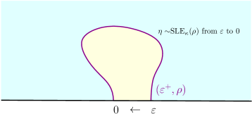
Figure 3. Illustration of Theorem 2.1: $\mathrm{SLE}^{\mathrm{bubble}}_{\kappa,0}(\rho)$ as the weak limit of chordal $\mathrm{SLE}_{\kappa}(\rho)$ with suitable rescaling.

Theorem 2.1 ([Zha22, Theorem $3.20$]).

Let $0<\kappa<4$ and $\rho>-2$. There exists a non-zero $\sigma$-finite measure $\mathrm{SLE}_{\kappa,0}^{\mathrm{bubble}}(\rho)$ on $\mathrm{Bubble}_{\mathbb{H}}(0)$ such that the following holds: For any fixed $S>0$, let $E_{S}=\{\eta:\mathrm{rad}_{0}(\eta)>S\}$. Then as $\varepsilon\to 0^{+}$,

(2.2.5) $$\varepsilon^{\frac{(\rho+2)(\kappa-8-2\rho)}{2\kappa}}\mathbbm{1}_{E_{S}}\mathrm{SLE}^{\mathbb{H}}_{\kappa,(\varepsilon;\varepsilon^{+})\to 0}(\rho)\xrightarrow{w}\mathbbm{1}_{E_{S}}\mathrm{SLE}_{\kappa,0}^{\mathrm{bubble}}(\rho)$$

in the space $\widetilde{\Sigma}^{\mathbb{C}}$ with distance defined by (2.2.4).

Remark 2.2.

Notice that in [AHS21, Theorem 3.20], the author considered $\mathrm{SLE}^{\mathbb{H}}_{\kappa,(r,r^{+})\to-r}(\rho)$ for $r>0$ as the limiting sequence of measures. To get (2.2.5), we first apply the shift map $f_{r}:\mathbb{H}\to\mathbb{H}$ such that $f_{r}(z)=z+r$ then let $\varepsilon=2r$.

Definition 2.3 (Rooted $\mathrm{SLE}_{\kappa}(\rho)$ bubble measures).

For $0<\kappa<4$ and $\rho>-2$, we define the weak limit $\mathrm{SLE}_{\kappa,0}^{\mathrm{bubble}}(\rho)$ in Theorem 2.1 as the rooted $\mathrm{SLE}_{\kappa}(\rho)$ bubble measure with root $0$. More generally, for any $p\in\partial\mathbb{H}$, let $f_{p}:\mathbb{H}\to\mathbb{H}$ be such that $f_{p}(z)=z+p$ and define

$$\mathrm{SLE}_{\kappa,p}^{\mathrm{bubble}}(\rho):=f_{p}(\mathrm{SLE}_{\kappa,0}^{\mathrm{bubble}}(\rho)).$$

If $\rho=0$, then we omit the existence of $\rho$ and write $\mathrm{SLE}_{\kappa,p}^{\mathrm{bubble}}$ for fixed $p\in\partial\mathbb{H}$.

Corollary 2.4.

Let $\widetilde{E_{i,0}}$ be the set of curves on $\overline{\mathbb{H}}$ starting from some point on $[0,\infty]$, ending at $0$, and surrounding $i$. Under the same settings as Theorem 2.1, we have

(2.2.6) $$\mathrm{SLE}^{\mathbb{H}}_{\kappa,(\varepsilon;\varepsilon^{+})\to 0}(\rho)[d\eta|\widetilde{E_{i,0}}]\xrightarrow{w}\mathrm{SLE}_{\kappa,0}^{\mathrm{bubble}}(\rho)[d\eta|\widetilde{E_{i,0}}]\qquad\text{as $\varepsilon\to 0^{+}$}$$

in the metric space $\widetilde{\Sigma}^{\mathbb{C}}$ with distance defined by (2.2.4).

Proof.

Let $E_{1}=\{\eta:\mathrm{rad}_{0}(\eta)>1\}$. It is clear that $\widetilde{E_{i,0}}\subset E_{1}$. Moreover, $\widetilde{E_{i,0}}$ is open in $\widetilde{\Sigma}^{\mathbb{C}}$ and $\partial\widetilde{E_{i,0}}$ contains the curves that end at $0$ and pass through $i$. For $0<\delta<1$, let $E_{\delta}=\{\eta:\mathrm{rad}_{0}(\eta)\geq\delta\}$ and $\tau_{\delta}=\inf_{t>0}\{t:\mathrm{rad}_{0}(\eta[0,t])=\delta\}$ be the first time that $\mathrm{SLE}_{\kappa,0}^{\mathrm{bubble}}(\rho)$ curve has radius $\delta$ under capacity parametrization. For any $\eta\in E_{\delta}$, let $\eta_{\delta}=\eta[0,\tau_{\delta}]$. For any fixed instance of $\eta_{\delta}$, let $\widetilde{\partial E_{i,\eta_{\delta}}}$ be the set of curves from $\eta(\tau_{\delta})$ to $0$ on $\mathbb{H}\backslash\eta_{\delta}$ that pass through $i$. By Domain Markov Property of $\mathrm{SLE}_{\kappa,0}^{\mathrm{bubble}}(\rho)$ stated in [Zha22, Theorem 3.16], we have that

(2.2.7) $$\begin{split}\mathrm{SLE}_{\kappa,0}^{\mathrm{bubble}}(\rho)[\partial\widetilde{E_{i,0}}]=\int_{E_{\delta}}\mathrm{SLE}_{\kappa,(\eta_{\delta},v(\eta_{\delta}))\to 0}^{\mathbb{H}\backslash\eta_{\delta}}(\rho)[\widetilde{\partial E_{i,\eta_{\delta}}}]\mathrm{SLE}_{k,0}^{\mathrm{bubble}}(\rho)(d\eta_{\delta}).\end{split}$$

By [Zha22, Theorem 3.20], $\mathrm{SLE}_{\kappa,0}^{\mathrm{bubble}}(\rho)[E_{\delta}]>0$. Moreover, it is well-known that when $0<\kappa<4$, the probability that chordal $\mathrm{SLE}_{\kappa}(\rho)$ passes through a fixed interior point is zero (see, for instance, [Zha19]). Therefore, $\mathrm{SLE}_{\kappa,0}^{\mathrm{bubble}}(\rho)[\partial\widetilde{E_{i,0}}]=0$. By (2.2.5) and [Zha22, (F3)],

(2.2.8) $$\varepsilon^{\frac{(\rho+2)(\kappa-8-2\rho)}{2\kappa}}\mathbbm{1}_{E_{1}}\mathbbm{1}_{\widetilde{E_{i,0}}}\mathrm{SLE}^{\mathbb{H}}_{\kappa,(\varepsilon;\varepsilon^{+})\to 0}(\rho)\xrightarrow{w}\mathbbm{1}_{E_{1}}\mathbbm{1}_{\widetilde{E_{i,0}}}\mathrm{SLE}_{\kappa,0}^{\mathrm{bubble}}(\rho).$$

Equivalently,

(2.2.9) $$\varepsilon^{\frac{(\rho+2)(\kappa-8-2\rho)}{2\kappa}}\mathbbm{1}_{\widetilde{E_{i,0}}}\mathrm{SLE}^{\mathbb{H}}_{\kappa,(\varepsilon;\varepsilon^{+})\to 0}(\rho)\xrightarrow{w}\mathbbm{1}_{\widetilde{E_{i,0}}}\mathrm{SLE}_{\kappa,0}^{\mathrm{bubble}}(\rho).$$

In order to prove (2.2.6), it remains to show that $0<\mathrm{SLE}_{\kappa,0}^{\mathrm{bubble}}(\rho)[\widetilde{E_{i,0}}]<\infty$. By [Zha22, Theorem 3.16],

(2.2.10) $$\mathrm{SLE}_{\kappa,0}^{\mathrm{bubble}}(\rho)[\widetilde{E_{i,0}}]\leq\mathrm{SLE}_{\kappa,0}^{\mathrm{bubble}}(\rho)[E_{1}]<\infty.$$

For any $\eta\in E_{\delta}$, let $\eta_{\delta}=\eta[0,\tau_{\delta}]$. For any fixed instance of $\eta_{\delta}$, let $\widetilde{E_{i,\eta_{\delta}}}$ denote the set of curves on $\mathbb{H}\backslash\eta_{\delta}$ from $\eta(\tau_{\delta})$ to $0$ that surround $i$. Again, by Domain Markov Property of $\mathrm{SLE}_{\kappa,0}^{\mathrm{bubble}}(\rho)$ ([Zha22, Theorem 3.16]),

(2.2.11) $$\begin{split}\mathrm{SLE}_{\kappa,0}^{\mathrm{bubble}}(\rho)[\widetilde{E_{i,0}}]=\int_{E_{\delta}}\mathrm{SLE}_{\kappa,(\eta_{\delta},v(\eta_{\delta}))\to 0}^{\mathbb{H}\backslash\eta_{\delta}}(\rho)[\widetilde{E_{i,\eta_{\delta}}}]\mathrm{SLE}_{k,0}^{\mathrm{bubble}}(\rho)(d\eta_{\delta}),\end{split}$$

where the force point $v(\eta_{\delta})$ is defined in [Zha22, (3.17)]. For each instance of $\eta_{\delta}$, we claim that

(2.2.12) $$\mathrm{SLE}_{\kappa,(\eta_{\delta},v(\eta_{\delta}))\to 0}^{\mathbb{H}\backslash\eta_{\delta}}(\rho)[\widetilde{E_{i,\eta_{\delta}}}]>0.$$

Assume otherwise, i.e., $\mathrm{SLE}_{\kappa,(\eta_{\delta},v(\eta_{\delta}))\to 0}^{\mathbb{H}\backslash\eta_{\delta}}(\rho)[\widetilde{E_{i,\eta_{\delta}}}]=0$. By conformal invariance property of chordal $\mathrm{SLE}_{\kappa}(\rho)$, we only need to consider the $\mathrm{SLE}_{\kappa}(\rho)$ on $\mathbb{H}$ from $0$ to $\infty$ conditional on passing to the left of $i$. By scaling property of chordal $\mathrm{SLE}_{\kappa}(\rho)$, the probability that $\mathrm{SLE}_{\kappa}(\rho)$ conditional on passing to the left of $ai,a>0$ is zero, i.e., $\mathrm{SLE}_{\kappa}(\rho)$ will almost surely stay to the right of positive imaginary axis. This is impossible and leads to a contradiction. Therefore, $\mathrm{SLE}_{\kappa,0}^{\mathrm{bubble}}(\rho)[\widetilde{E_{i,0}}]>0$ and this completes the proof. ∎

2.3. The Liouville Conformal Field Theory

In this section, we review key results of Liouville Conformal Field Theory on $\mathbb{H}$.

2.3.1. Definitions of the LCFT

To start, let $h$ be the centered Gaussian process on $\mathbb{H}$ with covariance kernel given by

$$\mathbb{E}[h(x)h(y)]=G_{\mathbb{H}}(x,y):=\log\frac{1}{|x-y||x-\overline{y}|}+2\log|x|_{+}+2\log|y|_{+},$$

where $|x|_{+}=\max(|x|,1)$. Notice that $h\in H^{-1}(\mathbb{H})$ and for test functions $f,g\in H^{1}(\mathbb{H})$, $(h,f)$ and $(h,g)$ are centred Gaussian variables with covariance given by

$$\mathbb{E}[(h,f),(h,g)]=\iint f(x)G_{\mathbb{H}}(x,y)g(y)d^{2}xd^{2}y.$$

Let $P_{\mathbb{H}}$ denote the law of $h$. For smooth test functions $f$ and $g$ with mean $0$ on $\mathbb{H}$, i.e.,

$$\int_{\mathbb{H}}f(z)d^{2}z=\int_{\mathbb{H}}g(z)d^{2}z=0,$$

we have that

$$\mathbb{E}[(h,f),(h,g)]=\frac{1}{2\pi}\int_{\mathbb{H}}\nabla f(z)\cdot\nabla g(z)d^{2}z.$$

Notice that this characterizes the free boundary Gaussian free field, which is defined modulo an additive constant. We can fix a particular instance of field $h$ by requiring the average around the upper half plane unit circle to be zero.

Given a function $f\in H^{-1}(\mathbb{H})$, let $f_{\varepsilon}(z)$ be the circular average of $f(z)$ over $\partial B(z,\varepsilon)\cap\mathbb{H}$. Suppose $h$ is sampled from $P_{\mathbb{H}}$, then we can define the random measures

$$\mu_{h}:=\lim_{\varepsilon\to 0}\varepsilon^{\gamma^{2}/2}e^{\gamma h_{\varepsilon}(z)}d^{2}z\qquad\text{and}\qquad\nu_{h}:=\lim_{\varepsilon\to 0}\varepsilon^{\gamma^{2}/4}e^{\gamma h_{\varepsilon}(z)/2}dz,$$

where convergence holds almost surely. We call $\mu_{h}$ the quantum area measure and $\nu_{h}$ the quantum boundary length measure.

Definition 2.5 ([AHS21, Definition 2.14]).

Let $(h,\mathbf{c})$ be sampled from $P_{\mathbb{H}}\times[e^{-Qc}dc]$ on the product space $H^{-1}(\mathbb{H})\times\mathbb{R}$. Let $\phi(z)=h(z)-2Q\log|z|_{+}+\mathbf{c}$ and let $\mathrm{LF}_{\mathbb{H}}$ denote the law of $\phi(z)$ on $H^{-1}(\mathbb{H})$. We call the sample from $\mathrm{LF}_{\mathbb{H}}$ the Liouville field.

Lemma 2.6 ([ARS22, Lemma 2.2]).

For $\alpha\in\mathbb{R}$ and $z_{0}\in\mathbb{H}$, the limit

$$\mathrm{LF}_{\mathbb{H}}^{(\alpha,z_{0})}:=\lim_{\varepsilon\to 0}\varepsilon^{\alpha^{2}/2}e^{\alpha\phi_{\varepsilon}(z_{0})}\mathrm{LF}_{\mathbb{H}}(d\phi)$$

exists in the vague topology. Moreover, sample $(h,\mathbf{c})$ from $(2\Im z_{0})^{-\alpha^{2}/2}|z_{0}|_{+}^{-2\alpha(Q-\alpha)}P_{\mathbb{H}}\times\left[e^{(\alpha-Q)c}dc\right]$ and let

$$\phi(z)=h(z)-2Q\log|z|_{+}+\alpha G_{\mathbb{H}}(z,z_{0})+\mathbf{c}\qquad\text{for $z\in\mathbb{H}$},$$

then the law of $\phi$ is given by $\mathrm{LF}_{\mathbb{H}}^{(\alpha,z_{0})}$. We call $\mathrm{LF}_{\mathbb{H}}^{(\alpha,z_{0})}$ the Liouville field on $\mathbb{H}$ with $\alpha$-insertion at $z$.

Next, we introduce the definition of Liouville field with multiple boundary insertions. The following definition is the combination of [AHS21, Definition 2.15] and [AHS21, Definition 2.17]:

Definition 2.7.

Let $(\beta_{i},s_{i})\in\mathbb{R}\times\partial\mathbb{H}$ for $i=1,\ldots,m$, where $m\geq 0$ and $s_{i}$ are pairwise distinct. Let $(h,\mathbf{c})$ be sampled from $C_{\mathbb{H}}^{(\beta_{i},s_{i})_{i}}P_{\mathbb{H}}\times\left[e^{(\frac{1}{2}\sum_{i}\beta_{i}-Q)c}dc\right]$, where

$$C_{\mathbb{H}}^{(\beta_{i},s_{i})_{i}}=\begin{cases}\prod_{i=1}^{m}|s_{i}|_{+}^{-\beta_{i}(Q-\frac{\beta_{i}}{2})}e^{\sum_{j=i+1}^{m}\frac{\beta_{i}\beta_{j}}{4}G_{\mathbb{H}}(s_{i},s_{j})}&\qquad\text{if $s_{1}\neq\infty$,}\\ \prod_{i=2}^{m}|s_{i}|_{+}^{-\beta_{i}(Q-\frac{\beta_{i}}{2}-\frac{\beta_{1}}{2})}e^{\sum_{j=i+1}^{m}\frac{\beta_{i}\beta_{j}}{4}G_{\mathbb{H}}(s_{i},s_{j})}&\qquad\text{if $s_{1}=\infty$.}\end{cases}$$

Let

$$\phi(z)=\begin{cases}h(z)-2Q\log|z|_{+}+\sum_{i=1}^{m}\frac{\beta_{i}}{2}G_{\mathbb{H}}(z,s_{i})+\mathbf{c}&\qquad\text{if $s_{1}\neq\infty$,}\\ h(z)+(\beta_{1}-2Q)\log|z|_{+}+\sum_{i=2}^{m}\frac{\beta_{i}}{2}G_{\mathbb{H}}(z,s_{i})+\mathbf{c}&\qquad\text{if $s_{1}=\infty$.}\end{cases}$$

We write $\mathrm{LF}_{\mathbb{H}}^{(\beta_{i},s_{i})_{i}}$ for the law of $\phi$ and call a sample from $\mathrm{LF}_{\mathbb{H}}^{(\beta_{i},s_{i})_{i}}$ the Liouville field on $\mathbb{H}$ with boundary insertions $(\beta_{i},s_{i})_{1\leq i\leq m}$.

Lemma 2.8 ([AHS21, Lemma 2.18]).

We have the following convergence in the vague topology of measures on $H^{-1}(\mathbb{H})$:

$$\lim_{r\to+\infty}r^{\beta(Q-\frac{\beta}{2})}\mathrm{LF}_{\mathbb{H}}^{(\beta,r),(\beta_{i},s_{i})_{i}}=\mathrm{LF}_{\mathbb{H}}^{(\beta,\infty),(\beta_{i},s_{i})_{i}}.$$

Definition 2.9.

Let $(\alpha,q)\in\mathbb{R}\times\mathbb{H}$ and let $(\beta_{i},p_{i})\in\mathbb{R}\times\partial\mathbb{H}$ for $1\leq i\leq m$. Suppose $(h,\mathbf{c})$ is sampled from $C_{\mathbb{H}}^{(\beta_{i},p_{i})_{i},(\alpha,q)}P_{\mathbb{H}}\times\left[e^{\left(\frac{1}{2}\sum_{i}\beta_{i}+\alpha-Q\right)c}dc\right]$, where

$$C_{\mathbb{H}}^{(\beta_{i},p_{i})_{i},(\alpha,q)}=\begin{cases}\prod_{i=1}^{m}|p_{i}|_{+}^{-\beta_{i}(Q-\frac{\beta_{i}}{2})}e^{\sum_{j=i+1}^{m}\frac{\beta_{i}\beta_{j}}{4}G_{\mathbb{H}}(p_{i},p_{j})}(2\Im q)^{-\frac{\alpha^{2}}{2}}|q|_{+}^{-2\alpha(Q-\alpha)}&\qquad\text{if $p_{1}\neq\infty$,}\\ \prod_{i=2}^{m}|p_{i}|_{+}^{-\beta_{i}(Q-\frac{\beta_{i}}{2}-\frac{\beta_{1}}{2})}e^{\sum_{j=i+1}^{m}\frac{\beta_{i}\beta_{j}}{4}G_{\mathbb{H}}(p_{i},p_{j})}(2\Im q)^{-\frac{\alpha^{2}}{2}}|q|_{+}^{-2\alpha(Q-\alpha)}&\qquad\text{if $p_{1}=\infty$.}\end{cases}$$

Let

$$\phi(z)=\begin{cases}h(z)-2Q\log|z|_{+}+\alpha G_{\mathbb{H}}(z,q)+\sum_{i=1}^{m}\frac{\beta_{i}}{2}G_{\mathbb{H}}(z,p_{i})+\mathbf{c}&\qquad\text{if $p_{1}\neq\infty$,}\\ h(z)+(\beta_{1}-2Q)\log|z|_{+}+\alpha G_{\mathbb{H}}(z,q)+\sum_{i=2}^{m}\frac{\beta_{i}}{2}G_{\mathbb{H}}(z,p_{i})+\mathbf{c}&\qquad\text{if $p_{1}=\infty$.}\end{cases}$$

We denote the law of $\phi(z)$ on $H^{-1}(\mathbb{H})$ by $\mathrm{LF}_{\mathbb{H}}^{(\beta_{i},p_{i})_{i},(\alpha,q)}$.

Finally, we recall the definition of the LCFT on horizontal strip $\mathcal{S}=\mathbb{R}\times(0,\pi)$. It is essentially the same procedure as defining LCFT on $\mathbb{H}$. Let

$$G_{\mathcal{S}}(z,w)=-\log|e^{z}-e^{w}|-\log|e^{z}-e^{\overline{w}}|+\max(2\Re z,0)+\max(2\Re w,0)$$

be the Green function on $\mathcal{S}$.

Definition 2.10 ([AHS21, Definition 2.19]).

Let $(h,\mathbf{c})$ be sampled from $C_{\mathcal{S}}^{(\beta,\pm\infty),(\beta_{3},s_{3})}P_{\mathcal{S}}\times\left[e^{(\beta+\frac{\beta_{3}}{2}-Q)c}dc\right]$, where $\beta\in\mathbb{R}$ and $(\beta_{3},s_{3})\in\mathbb{R}\times\partial\mathcal{S}$, and

$$C_{\mathcal{S}}^{(\beta,\pm\infty),(\beta_{3},s_{3})}=e^{(-\frac{\beta_{3}}{2}(Q-\frac{\beta_{3}}{2})+\frac{\beta\beta_{3}}{2})|\Re s_{3}|}.$$

Let $\phi(z)=h(z)-(Q-\beta)|\Re z|+\frac{\beta_{3}}{2}G_{\mathcal{S}}(z,s_{3})+\mathbf{c}$ and we denote the law of $\phi(z)$ on $H^{-1}(\mathbb{H})$ by $\mathrm{LF}_{\mathcal{S}}^{(\beta,\pm\infty),(\beta_{3},s_{3})}$.

2.3.2. Conformal symmetries of LCFT

Let $\mathrm{conf}(\mathbb{H})$ be the group of conformal automorphisms of $\mathbb{H}$ where group multiplication $\cdot$ is the function composition $f\cdot g=f\circ g$.

Proposition 2.11 ([AHS21, Proposition $2.16$]).

For $\beta\in\mathbb{R}$, let $\Delta_{\beta}=\frac{\beta}{2}(Q-\frac{\beta}{2})$. Let $f\in\mathrm{conf}(\mathbb{H})$ and $(\beta_{i},s_{i})\in\mathbb{R}\times\partial\mathbb{H}$ with $f(s_{i})\neq\infty$ for all $1\leq i\leq m$. Then $\mathrm{LF}_{\mathbb{H}}=f_{*}(\mathrm{LF}_{\mathbb{H}})$ and

$$\mathrm{LF}_{\mathbb{H}}^{(\beta_{i},f(s_{i}))_{i}}=\prod_{i=1}^{m}|f^{\prime}(s_{i})|^{-\Delta_{\beta_{i}}}f_{*}\left(\mathrm{LF}_{\mathbb{H}}^{(\beta_{i},s_{i})_{i}}\right).$$

Proposition 2.12.

For $1\leq i\leq m$ and $1\leq j\leq n$, let $(\alpha_{i},z_{i})\in\mathbb{R}\times\mathbb{H}$ and $(\beta_{j},s_{j})\in\mathbb{R}\times\partial\mathbb{H}$ with $f(s_{j})\neq\infty$ for all $1\leq j\leq n$. Let $f\in\mathrm{conf}(\mathbb{H})$ and we have

$$\mathrm{LF}_{\mathbb{H}}^{(\alpha_{i},f(z_{i}))_{i},(\beta_{j},f(s_{j}))_{j}}=\prod_{i=1}^{m}\prod_{j=1}^{n}|f^{\prime}(z_{i})|^{-2\Delta_{\alpha_{i}}}|f^{\prime}(s_{j})|^{-\Delta_{\beta_{j}}}\mathrm{LF}_{\mathbb{H}}^{(\alpha_{i},z_{i})_{i},(\beta_{j},s_{j})_{j}}.$$

Proof.

The proof is exactly the same as that of [AHS21, Proposition 2.9], which describes the case in $\widehat{\mathbb{C}}$ instead of $\mathbb{H}$. ∎

Lemma 2.13 ([ARS22, Lemma 3.14]).

Let $\alpha\in\mathbb{R}$ and $u\in\mathcal{S}$ with $\Re(u)=0$, then we have

$$\exp_{*}\mathrm{LF}_{\mathcal{S}}^{(\alpha,u)}=\mathrm{LF}_{\mathbb{H}}^{(\alpha,e^{u})}.$$

Lemma 2.14 ([AHS21, Lemma 2.20]).

Let $\beta\in\mathbb{R}$ and $(\beta_{3},s_{3})\in\mathbb{R}\times\partial\mathcal{S}$, then we have

$$\mathrm{LF}_{\mathbb{H}}^{(\beta,\infty),(\beta,0),(\beta_{3},e^{s_{3}})}=e^{\frac{\beta_{3}^{2}}{4}\Re s_{3}}\exp_{*}\mathrm{LF}_{\mathcal{S}}^{(\beta,\pm\infty),(\beta_{3},s_{3})}.$$

Similarly, if $\beta_{1},\beta_{2},\beta_{3}\in\mathbb{R}$ and $f\in\mathrm{conf}(\mathbb{H})$ satisfies $f(0)=0,f(1)=1,$ and $f(-1)=\infty$, then

$$\mathrm{LF}_{\mathbb{H}}^{(\beta_{1},\infty),(\beta_{2},0),(\beta_{3},1)}=2^{\Delta_{\beta_{1}}-\Delta_{\beta_{2}}+\Delta_{\beta_{3}}}\cdot f_{*}\mathrm{LF}_{\mathbb{H}}^{(\beta_{1},-1),(\beta_{2},0),(\beta_{3},1)}.$$

2.4. Quantum disks

2.4.1. Quantum surfaces

Let $\mathcal{D}\mathcal{H}=\{(D,h):D\subset\mathbb{C}\ \text{open, $h\in C_{0}^{\infty}(D)^{\prime}$}\}$. We define equivalence relation on $\mathcal{D}\mathcal{H}$ by letting $(D,h)\sim(\widetilde{D},\widetilde{h})$ if there is a conformal map $\psi:D\to\widetilde{D}$ such that $\widetilde{h}=\psi\bullet_{\gamma}h$, where

(2.4.1) $$\psi\bullet_{\gamma}h:=h\circ\psi^{-1}+Q\log|(\psi^{-1})^{\prime}|.$$

A quantum surface is an equivalence class of pairs $(D,h)\in\mathcal{D}\mathcal{H}$ under the equivalence relation $\sim_{\gamma}$. An embedding of a quantum surface is a choice of representative $(D,h)$. We can also consider quantum surfaces with marked points $(D,h,z_{1},\ldots,z_{m},\omega_{1},\ldots,\omega_{n})$ where $z_{i}\in D$ and $\omega_{j}\in\partial D$. We say

$$(D,h,z_{1},\ldots,z_{m},\omega_{1},\ldots,\omega_{n})\sim_{\gamma}(\widetilde{D},\widetilde{h},\widetilde{z_{1}},\ldots,\widetilde{z_{m}},\widetilde{\omega_{1}},\ldots,\widetilde{\omega_{n}})$$

if there is a conformal map $\psi:D\to\widetilde{D}$ such that $\widetilde{h}=\psi\bullet_{\gamma}h$ and $\psi(z_{i})=\widetilde{z_{i}},\psi(\omega_{j})=\widetilde{\omega_{j}}$. Let $\mathscr{D}_{m,n}$ denote the set of equivalence class of such tuples under $\sim_{\gamma}$ and let $\mathscr{D}=\mathscr{D}_{0,0}$ for simplicity. We use $(\ref{quantum equivalence relation})$ to define the equivalence relation because $\gamma$-LQG quantum area and $\gamma$-LQG quantum length measure is invariant under pushforward $\bullet_{\gamma}$. Since we will mainly work with $\mathbb{H}$, we view the set $\mathscr{D}_{m,n}$ as the quotient space

$$\{(\mathbb{H},h,z_{1},\ldots,z_{m},\omega_{1},\ldots,\omega_{n}):h\ \text{is a distribution on $\mathbb{H}$},z_{1}\ldots,z_{m}\in\mathbb{H},\omega_{1},\ldots,\omega_{n}\in\overline{\mathbb{R}}\}/\sim_{\gamma}.$$

The Borel $\sigma$-algebra of $\mathscr{D}_{m,n}$ is induced by the Borel sigma algebra on $H^{-1}(\mathbb{H})$.

2.4.2. Quantum Disks

We recall the definitions of two-pointed quantum disk introduced in [AHS20]. It is a family of measures on $\mathscr{D}_{0,2}$. It is initially defined on the horizontal strip $\mathcal{S}=\mathbb{R}\times(0,\pi)$. Let $\exp:\mathcal{S}\to\mathbb{H}$ be the exponential map $z\mapsto e^{z}$ and let $h_{\mathcal{S}}=h_{\mathbb{H}}\circ\exp$ where $h_{\mathbb{H}}$ is sampled from $P_{\mathbb{H}}$. We call $h_{\mathcal{S}}$ the free boundary GFF on $\mathcal{S}$. It is known that $h_{\mathcal{S}}$ can be written as the sum of $h^{c}$ and $h^{\ell}$ where $h^{c}$ is constant on $u+[0,i\pi],u\in\mathbb{R}$ and $h^{\ell}$ has mean zero on all such vertical lines. We call $h^{\ell}$ the lateral component of free boundary GFF.

Definition 2.15 (Thick quantum disk).

Let $W\geq\frac{\gamma^{2}}{2}$, and let $\beta=Q+\frac{\gamma}{2}-\frac{W}{\gamma}$. Let

$$Y_{t}=\begin{cases}B_{2t}-(Q-\beta)t&\qquad\text{if $t\geq 0$,}\\ \widetilde{B_{-2t}}+(Q-\beta)t&\qquad\text{if $t<0$,}\end{cases}$$

where $(B_{s})_{s\geq 0},(\widetilde{B}_{s})_{s\geq 0}$ are independent standard Brownian motions conditional on $B_{2s}-(Q-\beta)s<0$ and $\widetilde{B_{2s}}-(Q-\beta)s<0$ for all $s>0$. Let $h^{1}(z)=Y_{t}$ for all $z$ with $\Re(z)=t$. Let $h^{2}(z)$ be the lateral component of free boundary GFF on $\mathcal{S}$ and let $\mathbf{c}$ be sampled from $\frac{\gamma}{2}e^{(\beta-Q)c}dc$ independent of $h^{1}$ and $h^{2}$. Let $\widehat{h}(z)=h^{1}(z)+h^{2}(z)$ and let $\phi(z)=\widehat{h}(z)+\mathbf{c}$. Let $\mathcal{M}^{\mathrm{disk}}_{0,2}(W)$ denote the infinite measure on $\mathscr{D}_{0,2}$ describing the law of $(\mathcal{S},\phi,-\infty,+\infty)$. We call a sample from $\mathcal{M}^{\mathrm{disk}}_{0,2}(W)$ a weight-$W$ quantum disk.

Theorem 2.16 ([AHS21, Theorem 2.22]).

Fix $W\geq\frac{\gamma^{2}}{2}$ and $\beta_{W}=\gamma+\frac{2-W}{\gamma}$. If we independently sample $T$ from $\mathrm{Leb}_{\mathbb{R}}$ and $(\mathcal{S},\phi,+\infty,-\infty)$ from $\mathcal{M}^{\mathrm{disk}}_{0,2}(W)$, then the law of $\widetilde{\phi}:=\phi(\cdot+T)$ is $\frac{\gamma}{2(Q-\beta_{W})^{2}}$ is $\frac{\gamma}{2(Q-\beta_{W})^{2}}\mathrm{LF}_{\mathcal{S}}^{(\beta_{W},\pm\infty)}$.

Definition 2.17.

For $W\geq\frac{\gamma^{2}}{2}$, we first sample $(\mathcal{S},\phi,+\infty,-\infty)$ from $\nu_{\phi}(\mathbb{R})\mathcal{M}^{\mathrm{disk}}_{0,2}(W)[d\phi]$, then sample $s\in\mathbb{R}$ according to the probability measure proportional to $\nu_{\phi}|_{\mathbb{R}}$. We denote the law of the surface $(\mathcal{S},\phi,+\infty,-\infty)/\sim_{\gamma}$ has the same law as $\mathcal{M}^{\mathrm{disk}}_{2,\bullet}(W)$.

Definition 2.18.

Fix $W\geq\frac{\gamma^{2}}{2}$ and let $\alpha\in\mathbb{R}$. Let $\mathcal{M}^{\mathrm{disk}}_{2,\bullet}(W;\alpha)$ denote the law of $(\mathcal{S},\phi,\pm\infty,0)/\sim_{\gamma}$ with $\phi$ sampled from $\frac{\gamma}{2(Q-\beta)^{2}}\mathrm{LF}_{\mathcal{S}}^{(\beta,\pm\infty),(\alpha,0)}$.

Definition 2.19 (Thin quantum disk).

Let $0<W<\frac{\gamma^{2}}{2}$ and define the infinite measure $\mathcal{M}^{\mathrm{disk}}_{0,2}(W)$ on two-pointed beaded surfaces as follows: first take $T$ according to $(1-\frac{2}{\gamma^{2}}W)^{-2}\mathrm{Leb}_{\mathbb{R}_{+}}$, then sample a Poisson point process $\{(u,\mathcal{D}_{u})\}$ according to $\mathrm{Leb}_{[0,T]}\times\mathcal{M}^{\mathrm{disk}}_{0,2}(\gamma^{2}-W)$ and concatenate the $\mathcal{D}_{u}$ according to ordering induced by $u$.

Definition 2.20.

For $W\in(0,\frac{\gamma^{2}}{2})$ and $\alpha\in\mathbb{R}$, let $(S_{1},S_{2},S_{3})$ be sampled from

$$\left(1-\frac{2}{\gamma^{2}}W\right)^{2}\mathcal{M}^{\mathrm{disk}}_{0,2}(W)\times\mathcal{M}^{\mathrm{disk}}_{2,\bullet}(\gamma^{2}-W;\alpha)\times\mathcal{M}^{\mathrm{disk}}_{0,2}(W)$$

and $S$ is the concatenation of the three surfaces. We define the infinite measure $\mathcal{M}^{\mathrm{disk}}_{2,\bullet}(W;\alpha)$ to be the law of $S$.

When $W=2$, two marked points of $\mathcal{M}^{\mathrm{disk}}_{0,2}(2)$ are typical with respect to the quantum boundary length measure, see [AHS20, Proposition $A.8$].

Definition 2.21 (Typical quantum disks).

Let $(\mathcal{S},\phi,-\infty,+\infty)$ be an embedding of a sample from $\mathcal{M}^{\mathrm{disk}}_{0,2}(2)$. Let $A=\mu_{\phi}(\mathcal{S})$ denote the total quantum area and $L=\nu_{\phi}(\partial\mathcal{S})$ denote the total quantum boundary length. Let $\mathrm{QD}$ denote the law of $(\mathcal{S},\phi)$ under reweighted measure $L^{-2}\mathcal{M}^{\mathrm{disk}}_{0,2}(2)$, viewed as a measure on $\mathscr{D}$ by forgetting two marked points. For non-negative integers $m$ and $n$, let $(\mathcal{S},\phi)$ be a sample from $A^{m}L^{n}\mathrm{QD}$, then independently sample $z_{1},\ldots,z_{m}$ and $\omega_{1},\ldots,\omega_{n}$ according to $\mu_{\phi}^{\#}$ and $\nu_{\phi}^{\#}$, respectively. Let $\mathrm{QD}_{m,n}$ denote the law of $(\mathcal{S},\phi,z_{1},\ldots,z_{m},\omega_{1},\ldots,\omega_{n})$ viewed as a measure on $\mathscr{D}_{m,n}$. We call a sample from $\mathrm{QD}_{m,n}$ quantum disk with $m$ bulk and $n$ boundary marked points.

2.4.3. Conformal welding of quantum disks

The following theorem describes the conformal welding of $n$ quantum disks. Notice that the weight $W$ is linearly added when performing the welding operation.

Theorem 2.22 ([AHS20, Theorem 2.2]).

Fix $W_{1},\ldots,W_{n}>0$ and $W=W_{1}+\ldots+W_{n}$. There exists a constant $C=C_{W_{1},\ldots,W_{n}}\in(0,\infty)$ such that for all $\ell,r>0$, the identity

(2.4.2) $$\begin{split}&\mathcal{M}^{\mathrm{disk}}_{0,2}(W;\ell,r)\otimes\mathcal{P}^{\mathrm{disk}}(W_{1},\ldots,W_{n})\\ &=C\iiint_{0}^{\infty}\mathcal{M}^{\mathrm{disk}}_{0,2}(W_{1};\ell,\ell_{1})\times\mathcal{M}^{\mathrm{disk}}_{0,2}(W_{2};\ell_{1},\ell_{2})\times\ldots\times\mathcal{M}^{\mathrm{disk}}_{0,2}(W_{n};\ell_{n-1},r)d\ell_{1}\ldots d\ell_{n-1}\end{split}$$

holds as measures on the space of curve-decorated quantum surfaces. The measure $\mathcal{P}^{\mathrm{disk}}(W_{1},\ldots,W_{n})$ is defined in [AHS20, Definition 2.25] on tuple of curves $(\eta_{1},\ldots,\eta_{n-1})$ in a domain $(D,x,y)$. It was defined by the following induction procedure: first sample $\eta_{n-1}$ from $\mathrm{SLE}_{\kappa}(W_{1}+\ldots+W_{n-1}-2;W_{n}-2)$ then $(\eta_{1},\ldots,\eta_{n-2})$ from $\mathcal{P}^{\mathrm{disk}}(W_{1},\ldots,W_{n-1})$ on connected component $(D^{\prime},x^{\prime},y^{\prime})$ on the left of $D\backslash\eta_{n-1}$ where $x^{\prime}$ and $y^{\prime}$ are the first and the last point hit by $\eta_{n-1}$.

3. Law of welding interface via a limiting procedure

In this section, we prove Proposition 3.1. In words, we show that under the same setup as Theorem 1.1, the law of the welding interface is $\mathrm{SLE}_{\kappa}(\rho)$ bubble measure conditioning on surrounding $i$.

Proposition 3.1.

Fix $\gamma\in(0,2)$. For $W>0$, let $\rho=W-2$. Let $(\mathbb{H},\phi,\eta,0,i)$ be an embedding of the quantum surface

(3.0.1) $$\int_{0}^{\infty}\mathcal{M}^{\mathrm{disk}}_{0,2}(W;\cdot,\ell)\times\mathrm{QD}_{1,1}(\ell)d\ell.$$

Let $M_{\phi}$ denote the marginal law of $\phi$ in $(\mathbb{H},\phi,\eta,0,i)$, then $(\phi,\eta)$ has the law of $M_{\phi}\times\mathrm{SLE}_{\kappa,0}^{\mathrm{bubble}}(\rho)[\cdot|i\in D_{\eta}(0)]$.

3.1. The LCFT description of three-pointed quantum disks

We start with the definition of two-pointed quantum disk with one additional typical bulk insertion.

Definition 3.2 ([ARS22, Definition 3.10]).

For $W\geq\frac{\gamma^{2}}{2}$, recall the definition of thick quantum disk $\mathcal{M}^{\mathrm{disk}}_{0,2}(W)$ from Definition 2.15. Sample $\phi$ on $H^{-1}(\mathbb{H})$ such that $(\mathbb{H},\phi,0,\infty)$ is an embedding of $\mathcal{M}^{\mathrm{disk}}_{0,2}(W)$. Let $L$ denote the law of $\phi$ and let $(\phi,z)$ be sampled from $L(d\phi)\mu_{\phi}(dz^{2})$. We write $\mathcal{M}^{\mathrm{disk}}_{1,2}(W)$ for the law $(\mathbb{H},\phi,z,0,\infty)$ viewed as a marked quantum surface.

Lemma 3.3.

For $\gamma\in(0,2)$ and $W\in\mathbb{R}$, let $\beta_{W}=\gamma+\frac{2-W}{\gamma}$. Suppose $(\phi,\mathbf{x})$ is sampled from $\mathrm{LF}_{\mathbb{H}}^{(\gamma,i),(\beta_{W},\infty),(\beta_{W},\mathbf{x})}\times dx$, then the law of $(\mathbb{H},\phi,\eta,i,\infty,\mathbf{x})$ as a marked quantum surface is equal to $\frac{2(Q-\beta_{W})^{2}}{\gamma}\mathcal{M}^{\mathrm{disk}}_{1,2}(W)$.

Proof.

By [ARS22, Lemma $3.12$], if $\mathcal{M}^{\mathrm{disk}}_{1,2}(W)$ is embedded as $(\mathcal{S},\phi,i\theta,+\infty,-\infty)$, then $(\phi,\theta)$ has the law of

(3.1.1) $$\frac{\gamma}{2(Q-\beta_{W})^{2}}\mathrm{LF}_{\mathcal{S}}^{(\beta_{W},\pm\infty),(\gamma,i\theta)}(d\phi)\mathbbm{1}_{\widetilde{\theta}\in(0,\pi)}d\widetilde{\theta}.$$

Fix $\theta\in(0,\pi)$ and let $\exp:\mathcal{S}\to\mathbb{H}$ be the map $z\mapsto e^{z}$. By [ARS22, Lemma $3.14$] and [AHS21, Lemma $2.20$], we have

$$\exp_{*}\left(\mathrm{LF}_{\mathcal{S}}^{(\beta_{W},\pm\infty),(\gamma,i\theta)}\right)=\mathrm{LF}_{\mathbb{H}}^{(\gamma,e^{i\theta}),(\beta_{W},\infty),(\beta_{W},0)}.$$

Let $f_{\theta}(z)=\frac{z}{\sin\theta}-\cot\theta$, which sends $e^{i\theta}\mapsto i$, $\infty\mapsto\infty$, and $0\mapsto\mathbf{x}=-\cot\theta$. By [AHS21, Proposition $2.16$], for any $r\in\mathbb{R}$, we have

$$\mathrm{LF}_{\mathbb{H}}^{(\gamma,i),(\beta_{W},-\cot\theta),(\beta_{W},\frac{r}{\sin\theta}-\cot\theta)}=(\sin\theta)^{2\Delta_{\gamma}+2\Delta_{\beta}}(f_{\theta})_{*}\mathrm{LF}_{\mathbb{H}}^{(\gamma,e^{i\theta}),(\beta_{W},0),(\beta_{W},r)},$$

where $\Delta_{\alpha}=\frac{\alpha}{2}(Q-\frac{\alpha}{2})$. After multiplying both sides by $\left(\frac{r}{\sin\theta}-\cot\theta\right)^{2\Delta_{\beta_{W}}}$, we have

$$\left(\frac{r}{\sin\theta}-\cot\theta\right)^{2\Delta_{\beta_{W}}}\mathrm{LF}_{\mathbb{H}}^{(\gamma,i),(\beta_{W},-\cot\theta),(\beta_{W},\frac{r}{\sin\theta}-\cot\theta)}$$

$$=(\sin\theta)^{2\Delta_{\gamma}+2\Delta_{\beta_{W}}}\left(\frac{1}{\sin\theta}-\frac{\cot\theta}{r}\right)^{2\Delta_{\beta_{W}}}\left(f_{\theta}\right)_{*}\left(r^{2\Delta_{\beta_{W}}}\mathrm{LF}_{\mathbb{H}}^{(\gamma,e^{\theta i}),(\beta_{W},0),(\beta_{W},r)}\right).$$

By [AHS21, Lemma $2.18$], taking limit as $r\to\infty$ yields

$$\frac{1}{(\sin\theta)^{2}}\mathrm{LF}_{\mathbb{H}}^{(\gamma,i),(\beta_{W},-\cot\theta),(\beta_{W},\infty)}=\left(f_{\theta}\right)_{*}\mathrm{LF}_{\mathbb{H}}^{(\gamma,e^{\theta i}),(\beta_{W},0),(\beta_{W},\infty)}.$$

Here the convergence is in the vague topology. When $\theta$ is sampled from $\mathbbm{1}_{(0,\pi)}(\widetilde{\theta})d\widetilde{\theta}$, we have

$$\frac{1}{(\sin\theta)^{2}}\mathrm{LF}_{\mathbb{H}}^{(\gamma,i),(\beta_{W},-\cot\theta),(\beta_{W},\infty)}=\mathrm{LF}_{\mathbb{H}}^{(\gamma,i),(\beta_{W},\infty),(\beta_{W},\mathbf{x})}\times dx$$

by change of variables $\mathbf{x}=-\cot\theta$. This completes the proof. ∎

A direct consequence of [AHS20, Theorem $2.2$] is the following:

Theorem 3.4.

Let $(\mathbb{H},\phi,0,\infty)$ be the embedding of a sample from $\mathcal{M}^{\mathrm{disk}}_{0,2}(W+2)$. Let $\eta$ be sampled from $\mathrm{SLE}_{\kappa}(W-2,0)$ on $(\mathbb{H},0,\infty)$ independent of $\phi$, then

(3.1.2) $$\mathcal{M}_{0,2}^{\mathrm{disk}}(W+2)\otimes\mathrm{SLE}_{\kappa}(W-2,0)=C_{W,2}\int_{0}^{\infty}\mathcal{M}_{0,2}^{\mathrm{disk}}(W,\cdot,\ell)\times\mathcal{M}^{\mathrm{disk}}_{0,2}(2,\ell,\cdot)d\ell$$

for some constant $C_{W,2}\in(0,\infty)$.

For $W>0$, let $\beta_{W+2}=\gamma-\frac{W}{\gamma}$. Let $(\phi,\mathbf{x})$ be sampled from $\mathrm{LF}_{\mathbb{H}}^{(\gamma,i),(\beta_{W+2},\infty),(\beta_{W+2},\mathbf{x})}\times dx$ and let $\eta$ be sampled from the chordal $\mathrm{SLE}^{\mathbb{H}}_{\kappa,(\mathbf{x};\mathbf{x}^{-})\to\infty}(W-2)$. Denote $\nu_{\phi}(a,b)$ the quantum boundary length of $(a,b)$ with respect to the random field $\phi$. Fix $\delta\in(0,\frac{1}{2})$ and let $M_{\delta}$ denote the law of $(\phi,\mathbf{x},\eta)$ restricted to the event that $\nu_{\phi}(\mathbf{x},\infty)\in(\delta,2\delta)$, $\nu_{\phi}(\mathbb{R})\in(1,2)$ and $i$ is to the right of $\eta$. Let $M_{\delta}^{\#}=\frac{1}{|M_{\delta}|}M_{\delta}$ be the corresponding probability measure.

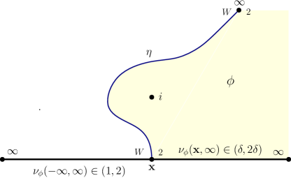
Figure 4. Illustration of $M_{\delta}$: first sample $(\phi,\mathbf{x})$ from $\mathrm{LF}_{\mathbb{H}}^{(\gamma,i),(\beta_{W+2},\infty),(\beta_{W+2},\mathbf{x})}\times dx$ and then sample $\eta$ according to $\mathrm{SLE}^{\mathbb{H}}_{\kappa,(\mathbf{x};\mathbf{x}^{-})\to\infty}(W-2)$. The $M_{\delta}$ is the restriction $(\phi,\mathbf{x},\eta)$ to the event that $\nu_{\phi}(\mathbf{x},\infty)\in(\delta,2\delta)$, $\nu_{\phi}(-\infty,\infty)\in(1,2)$ and $i$ is to the right of $\eta$.

Lemma 3.5.

Fix $W>0$. There exists some constant $C\in(0,\infty)$ such that for each $\delta\in(0,\frac{1}{2})$, if $(\phi,\mathbf{x},\eta)$ is sampled from $M_{\delta}$, then the law of marked quantum surface $(\mathbb{H},\phi,\eta,i,\mathbf{x},\infty)$ is

(3.1.3) $$C\cdot\int_{\delta}^{2\delta}\int_{1-\ell^{\prime}}^{2-\ell^{\prime}}\int_{0}^{\infty}\mathcal{M}_{0,2}^{\mathrm{disk}}(W;\ell,\ell_{1})\times\mathcal{M}^{\mathrm{disk}}_{1,2}(2,\ell_{1},\ell^{\prime})d\ell_{1}d\ell d\ell^{\prime}.$$

Proof.

By Lemma 3.3, if we sample $(\phi,\mathbf{x})$ from $\mathrm{LF}_{\mathbb{H}}^{(\gamma,i),(\beta_{W+2},\infty),(\beta_{W+2},\mathbf{x})}\times dx$, then $(\mathbb{H},\phi,i,\mathbf{x},\infty)$ viewed as a marked quantum surface has the law of $C\cdot\mathcal{M}_{1,2}^{\mathrm{disk}}(W+2)$ for some constant $C\in(0,\infty)$. Furthermore, if we sample $\eta$ from $\mathrm{SLE}^{\mathbb{H}}_{\kappa,(\mathbf{x};\mathbf{x}^{-})\to\infty}(W-2)$ conditional on $i$ is to the right of $\eta$, then by Theorem 3.4, the quantum surface $(\mathbb{H},\phi,\eta,i,\mathbf{x},\infty)$ has the law of

(3.1.4) $$C\cdot\int_{0}^{\infty}\int_{0}^{\infty}\int_{0}^{\infty}\mathcal{M}_{0,2}^{\mathrm{disk}}(W;\ell,\ell_{1})\times\mathcal{M}_{1,2}^{\mathrm{disk}}(2;\ell_{1},\ell^{\prime})d\ell d\ell_{1}d\ell^{\prime}.$$

Conditioning on $\nu_{\phi}(\mathbf{x},\infty)\in(\delta,2\delta)$ and $\nu_{\phi}(\mathbb{R})\in(1,2)$ gives the desired result. ∎

3.2. Proof of Proposition 3.1 via coupling

Fix $W>0$. Sample a pair of quantum surfaces $(\mathcal{D}_{1},\mathcal{D}_{2})$ from

(3.2.1) $$\int_{1}^{2}\int_{0}^{\infty}\mathcal{M}^{\mathrm{disk}}_{0,2}(W;a,p)\times\mathrm{QD}_{1,1}(p)dpda$$

and let $\mathcal{D}_{1}\oplus\mathcal{D}_{2}$ be the curve-decorated quantum surface obtained by conformally welding the right boundary of $\mathcal{D}_{1}$ and total boundary of $\mathcal{D}_{2}$. Notice that $\mathcal{D}_{1}\oplus\mathcal{D}_{2}$ has a interior marked point and a boundary marked point. Let $(\mathbb{D},\phi_{\mathbb{D}},\eta_{\mathbb{D}},0,i)$ be the unique embedding of $\mathcal{D}_{1}\oplus\mathcal{D}_{2}$ on $(\mathbb{D},0,i)$ and let $f:\mathbb{H}\to\mathbb{D}$ be the conformal map with $f(i)=0$ and $f(\infty)=i$. Denote $M_{\mathbb{D}}$ the joint law of $(\mathbb{D},\phi_{\mathbb{D}},\eta_{\mathbb{D}},0,i)$ and let $M_{\mathbb{D}}^{\#}=\frac{1}{|M_{\mathbb{D}}|}M_{\mathbb{D}}$ be the probability measure obtained from $M_{\mathbb{D}}$.

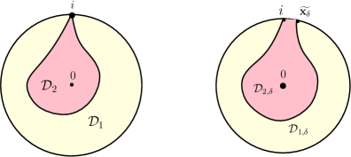
Figure 5. Left: $(\phi_{\mathbb{D}},\eta_{\mathbb{D}})$ from $M_{\mathbb{D}}^{\#}$ is obtained by embedding $\mathcal{D}_{1}\oplus\mathcal{D}_{2}$ into $(\mathbb{D},0,i)$. Right: $(\phi^{\delta},\eta^{\delta})$ from $M_{\delta}^{\#}$ is obtained by embedding $\mathcal{D}_{1,\delta}\oplus\mathcal{D}_{2,\delta}$ into $(\mathbb{D},0,i)$.

Next, we recall the definition of $M_{\delta}^{\#}$. For $0<\gamma<2$ and $W>0$, let $\beta_{W+2}=\gamma-\frac{W}{\gamma}$. Sample $(\phi,\mathbf{x})$ from $\mathrm{LF}_{\mathbb{H}}^{(\gamma,i),(\beta_{W+2},\infty),(\beta_{W+2},\mathbf{x})}\times dx$ and let $\eta$ be sampled from $\mathrm{SLE}^{\mathbb{H}}_{\kappa,(\mathbf{x};\mathbf{x}^{-})\to\infty}(W-2)$. Fix $\delta\in(0,\frac{1}{2})$ and let $M_{\delta}$ be the law of $(\phi,\mathbf{x},\eta)$ restricted to the event that $\nu_{\phi}(\mathbf{x},\infty)\in(\delta,2\delta)$, $\nu_{\phi}(\mathbb{R})\in(1,2)$ and $i$ is to the right of $\eta$. Let $M_{\delta}^{\#}=\frac{1}{|M_{\delta}|}M_{\delta}$ be the corresponding probability measure.

Sample $(\phi,\mathbf{x},\eta)$ from $M_{\delta}^{\#}$ and let $\mathcal{D}_{1,\delta}$ and $\mathcal{D}_{2,\delta}$ be the two components such that $(\mathbb{H},\phi,\eta,i,\mathbf{x})$ is the embedding of the surface $\mathcal{D}_{1\,\delta}\oplus\mathcal{D}_{2,\delta}$ after conformal welding. Let $\phi^{\delta}=\phi\circ f^{-1}+\log|(f^{-1})^{\prime}|$ and $\eta^{\delta}=f\circ\eta$ be such that $(\mathbb{D},\phi^{\delta},\eta^{\delta},0,i)$ is the embedding of $\mathcal{D}_{1,\delta}\oplus\mathcal{D}_{2,\delta}$. Here $\eta^{\delta}$ is the welding interface between $\mathcal{D}_{1,\delta}$ and $\mathcal{D}_{2,\delta}$. Let $\widetilde{\mathbf{x}_{\delta}}=f(\mathbf{x})$ be the image of $\mathbf{x}$ under $f$.

Lemma 3.6.

There exists a coupling between $M_{\mathbb{D}}^{\#}$ and $M_{\delta}^{\#}$ such that the followings hold: There exist random simply connected domains $U_{\delta}$ and $\widetilde{U_{\delta}}\subset\mathbb{D}$ and a conformal map $g_{\delta}:\widetilde{U_{\delta}}\to U_{\delta}$ satisfying the following properties: With probability $1-o_{\delta}(1)$, we have

1. $\phi_{\mathbb{D}}(z)=\phi^{\delta}\circ g_{\delta}(z)+Q\log|g_{\delta}^{\prime}(z)|,\qquad\text{for $z\in\widetilde{U_{\delta}}$}.$

2. ${\mathrm{diam}}(\mathbb{D}\backslash U_{\delta})=o_{\delta}(1)\ \text{and}\ {\mathrm{diam}}(\mathbb{D}\backslash\widetilde{U_{\delta}})=o_{\delta}(1).$

3. $|\widetilde{\mathbf{x}_{\delta}}-i|=o_{\delta}(1).$

4. $\sup_{z\in K}|g_{\delta}(z)-z|=o_{\delta}(1),\ \ \text{for any compact set $K\subset\mathbb{D}$}.$

In order to prove Lemma 3.6, we need the following two basic coupling results on the quantum disk. The first one is on $\mathrm{QD}_{1,1}$. Suppose $\mathcal{D}$ as a quantum surface has the law of $\mathrm{QD}_{1,1}$ and it has emebdding $(\mathbb{H},\phi,i,-1)$. Let $\mathcal{D}^{\varepsilon}:=\left(\mathbb{H}_{\varepsilon},\phi,i,-1,-1-2\varepsilon\right)$, where $\mathbb{H}_{\varepsilon}=\mathbb{H}\backslash B_{\varepsilon}(-1-\varepsilon)$ with $B_{\varepsilon}(-1-\varepsilon)=\left\{z\in\mathbb{C}:|z+1+\varepsilon|\leq\varepsilon\right\}$.

Lemma 3.7 ([ARS22, Lemma $5.17$]).

For $\varepsilon>0$ and $\ell>0$, suppose $\mathcal{D}$ and $\widetilde{\mathcal{D}}$ are sampled from $\mathrm{QD}_{1,1}(\ell)^{\#}$ and $\mathrm{QD}_{1,1}(\widetilde{\ell})^{\#}$ respectively, then the law of $\widetilde{\mathcal{D}^{\varepsilon}}$ converges in total variation distance to $\mathcal{D}^{\varepsilon}$ as $\widetilde{\ell}\to\ell$.

The second coupling result is on $\mathcal{M}^{\mathrm{disk}}_{0,2}(W)$. Suppose $\mathcal{D}$ is sampled from $\mathcal{M}^{\mathrm{disk}}_{0,2}(W)$ and it has embedding $(\mathbb{D},\phi,-i,i)$. With a slight abuse of notation, let $\mathcal{D}^{\varepsilon}:=(\mathbb{D}_{\varepsilon},\phi,\alpha_{\varepsilon},\alpha^{\prime}_{\varepsilon},i,-i)$, where $B_{\varepsilon}(i)=\left\{z\in\mathbb{C}:|z-i|\leq\varepsilon\right\}$, $\mathbb{D}_{\varepsilon}=\mathbb{D}\backslash B_{\varepsilon}(i)$, and $\{\alpha_{\varepsilon},\alpha^{\prime}_{\varepsilon}\}=\partial\mathbb{D}\cap\partial B_{\varepsilon}(i)$.

Lemma 3.8.

Fix $W>0$. For $\varepsilon,\ell,r,\widetilde{\ell},\widetilde{r}>0$, suppose $\mathcal{D}$ and $\widetilde{\mathcal{D}}$ are sampled from $\mathcal{M}^{\mathrm{disk}}_{0,2}(W;\ell,r)^{\#}$ and $\mathcal{M}^{\mathrm{disk}}_{0,2}(W;\widetilde{\ell},\widetilde{r})^{\#}$ respectively, then $\widetilde{\mathcal{D}^{\varepsilon}}$ converges in total variation distance to $\mathcal{D}$ as $(\widetilde{\ell},\widetilde{r})\to(\ell,r)$.

Proof.

The proof follows directly from [AHS20, Proposition $2.23$]. ∎

Lemma 3.9.

Suppose $(\phi,\mathbf{x},\eta)$ is sampled from $M_{\delta}^{\#}$ and let $A=\nu_{\phi}(-\infty,\mathbf{x})$, $B=\nu_{\phi}(\mathbf{x},\infty)$ and $P=\nu_{\phi}(\eta)$, then as $\delta\to 0$, $B$ converges to $0$ in probability and the $M_{\delta}^{\#}$-law of $(A,P)$ converges in total variation distance to a probability measure on $(1,2)\times(0,\infty)$ whose density function is proportional to

(3.2.2) $$f_{W}(a,p)p^{-\frac{4}{\gamma^{2}}+1}dadp,$$

where $f_{W}(a,p)=|\mathcal{M}^{\mathrm{disk}}_{0,2}(W;a,p)|$.

Proof.

By Proposition $5.1$ and [AHS21, Lemma $3.3$], we have

(3.2.3) $$|\mathcal{M}^{\mathrm{disk}}_{0,2}(W;\ell,r)|=f_{W}(\ell,r)\qquad\text{and}\qquad|\mathcal{M}^{\mathrm{disk}}_{1,2}(2;\ell,r)|=C(\ell+r)^{-\frac{4}{\gamma^{2}}+1}.$$

By $(\ref{welding equation})$, the $M_{\delta}^{\#}$-law of $(A,P,B)$ is a probability measure on the space

$$S_{\delta}=\left\{(a,p,b)\in(0,\infty)^{3}:b\in(\delta,2\delta),a+b\in(1,2)\right\},$$

whose density function is proportional to

$$m(a,p,b)=f_{W}(a,p)(p+b)^{-\frac{4}{\gamma^{2}}+1}.$$

Therefore, we have

$$|M_{\delta}|=\int_{S_{\delta}}m(a,p,b)dadpdb.$$

By definition of $M_{\delta}^{\#}$, for any $\varepsilon>0$, we have $\lim_{\delta\to 0}M_{\delta}^{\#}[B>\varepsilon]=0$. As $\delta\to 0$, the limiting $M_{\delta}^{\#}$-law of $(A,P)$ is a probability measure on $(1,2)\times(0,\infty)$ whose density function is proportional to $f_{W}(a,p)p^{-\frac{4}{\gamma^{2}}+1}$. This completes the proof. ∎

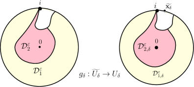
Figure 6. We can couple $M_{\mathbb{D}}^{\#}$ and $M_{\delta}^{\#}$ so that the light green and pink quantum surfaces agree with high probability. The domain $\widetilde{U_{\delta}}$ is the interior of $\overline{\mathcal{D}_{1}^{\varepsilon}\cup\mathcal{D}_{2}^{\varepsilon}}$ in the embedding of $\mathcal{D}_{1}\oplus\mathcal{D}_{2}$ and $U_{\delta}$ is the interior of $\overline{\mathcal{D}_{1,\delta}^{\varepsilon}\cup\mathcal{D}_{2,\delta}^{\varepsilon}}$ in the embedding of $\mathcal{D}_{1,\delta}\oplus\mathcal{D}_{2,\delta}$.

Proof of Lemma 3.6.

Recall the definition of marked quantum surfaces $\mathcal{D}_{1}$ and $\mathcal{D}_{2}$ embedded as $(\mathbb{D},\phi_{\mathbb{D}},\eta_{\mathbb{D}},0,i)$. Let $\widetilde{A}$ and $\widetilde{P}$ be the left and right boundary length of $\mathcal{D}_{1}$ respectively. The law of $(\widetilde{A},\widetilde{P})$ is the probability measure on $[1,2]\times(0,\infty)$ proportional to

(3.2.4) $$\left|\mathcal{M}^{\mathrm{disk}}_{0,2}(W;a,p)\right||\mathrm{QD}_{1,1}(p)|\propto f_{W}(a,p)p^{-\frac{4}{\gamma^{2}}+1}.$$

Conditioning on $(\widetilde{A},\widetilde{P})$, the joint law of $(\mathcal{D}_{1},\mathcal{D}_{2})$ is $\mathcal{M}^{\mathrm{disk}}_{0,2}(W;\widetilde{A},\widetilde{P})^{\#}\times\mathrm{QD}_{1,1}(\widetilde{P})^{\#}$.

Next, let $A_{\delta}$ and $P_{\delta}$ be the left and right boundary of $D_{1,\delta}$ respectively and let $B_{\delta}$ be the right boundary of $D_{2,\delta}$. By Lemma 3.9, as $\delta\to 0$, $M_{\delta}^{\#}$-law of $(A_{\delta},P_{\delta})$ converges in law to $(\widetilde{A},\widetilde{P})$ and $B_{\delta}\to 0$ in probability. Therefore, we can couple $M_{\delta}^{\#}$ and $M_{\mathbb{D}}^{\#}$ so that $(A_{\delta},P_{\delta})=(\widetilde{A},\widetilde{P})$ with probability $1-o_{\delta}(1)$. By Lemma 3.7 and 3.8, there exists a coupling between $(\mathcal{D}_{1}^{\varepsilon},\mathcal{D}_{2}^{\varepsilon})$ and $(\mathcal{D}_{1,\delta}^{\varepsilon},\mathcal{D}_{2,\delta}^{\varepsilon})$ such that

(3.2.5) $$\lim_{\delta\to 0}\mathbb{P}\left[(\mathcal{D}_{1}^{\varepsilon},\mathcal{D}_{2}^{\varepsilon})=(\mathcal{D}_{1,\delta}^{\varepsilon},\mathcal{D}_{2,\delta}^{\varepsilon})\right]=1$$

for some $\varepsilon=o_{\delta}(1)$ with sufficiently slow decay. Let $\widetilde{U_{\delta}}$ denote the interior of $\overline{\mathcal{D}_{1}^{\varepsilon}\cup\mathcal{D}_{2}^{\varepsilon}}$ in the embedding of $\mathcal{D}_{1}\oplus\mathcal{D}_{2}$ and $U_{\delta}$ denote the interior of $\overline{\mathcal{D}_{1,\delta}^{\varepsilon}\cup\mathcal{D}_{2,\delta}^{\varepsilon}}$ in the embedding of $\mathcal{D}_{1,\delta}\oplus\mathcal{D}_{2,\delta}$. By conformal welding, the marked quantum surfaces $(\widetilde{U_{\delta}},\phi_{\mathbb{D}},0,i^{-})$ and $(U_{\delta},\phi^{\delta},0,i^{-})$ agree with probability $1-o_{\delta}(1)$. On this high probability event, there exists a unique conformal map $g_{\delta}:\widetilde{U_{\delta}}\to U_{\delta}$ such that $\phi_{\mathbb{D}}=\phi^{\delta}\circ g_{\delta}+Q\log|g_{\delta}^{\prime}|$ with $g_{\delta}(0)=0$ and $g_{\delta}(i^{-})=i^{-}$.

Notice that the random simply connected domain $\widetilde{U_{\delta}}$ is completely determined by $M_{\mathbb{D}}^{\#}$. Almost surely under $M_{\mathbb{D}}^{\#}$, the $\{\overline{\mathbb{D}}\backslash\widetilde{U_{\delta}}\}_{\delta}$ is a sequence of shrinking compact sets in the euclidean sense, i.e., ${\mathrm{diam}}(\overline{\mathbb{D}}\backslash\widetilde{U_{\delta}})=o_{\delta}(1)$ and $\bigcap_{\delta>0}\overline{\mathbb{D}}\backslash\widetilde{U_{\delta}}=\{i\}$. By the coupling between $M_{\mathbb{D}}^{\#}$ and $M_{\delta}^{\#}$, we know that ${\mathrm{diam}}(\overline{\mathbb{D}}\backslash\widetilde{U_{\delta}})=o_{\delta}(1)$ with probability $1-o_{\delta}(1)$. Notice that ${\mathrm{diam}}(\overline{\mathbb{D}}\backslash\widetilde{U_{\delta}})=0$ if and only if the harmonic measure of $\mathbb{D}\backslash\widetilde{U_{\delta}}$ viewed from $0$ in $\widetilde{U_{\delta}}$ tends to $0$ as $\delta\to 0$. Therefore, in our coupling, with probability $1-o_{\delta}(1)$, the harmonic measure of $\mathbb{D}\backslash\widetilde{U_{\delta}}$ viewed from $0$ in $\widetilde{U_{\delta}}$ is $o_{\delta}(1)$. Since the harmonic measure is conformally invariant and by $(\ref{coupling equation})$, with probability $1-o_{\delta}(1)$, harmonic measure of $\mathbb{D}\backslash U_{\delta}$ viewed from $0$ in $U_{\delta}$ is also $o_{\delta}(1)$. Hence, we have ${\mathrm{diam}}(\mathbb{D}\backslash U_{\delta})=o_{\delta}(1)$ with probability $1-o_{\delta}(1)$. This proves $(2)$ in Lemma 3.6.

By construction, we know that $\widetilde{\mathbf{x}_{\delta}}\in\mathbb{D}\backslash U_{\delta}$ and $|\widetilde{\mathbf{x}_{\delta}}-i|\leq{\mathrm{diam}}\left(\mathbb{D}\backslash U_{\delta}\right)$. The above argument directly implies that $|\widetilde{\mathbf{x}_{\delta}}-i|=o_{\delta}(1)$ with probability $1-o_{\delta}(1)$. Therefore $(3)$ is also proved.

Finally, by $(\ref{coupling equation})$, we have that $g_{\delta}(0)=0$, $g_{\delta}(i^{-})=i^{-}$, ${\mathrm{diam}}(\mathbb{D}\backslash U_{\delta})=o_{\delta}(1)$, and ${\mathrm{diam}}(\mathbb{D}\backslash\widetilde{U_{\delta}})=o_{\delta}(1)$ with probability $1-o_{\delta}(1)$, the standard conformal distortion estimates imply $(4)$. ∎

Proof of Proposition 3.1.

For the convenience of readers, we first recall the definition and basic setup regarding $M^{\#}_{\delta}$ on $\mathbb{H}$: For $W>0$, let $\beta_{W+2}=\gamma-\frac{W}{\gamma}$. Sample $(\phi,\mathbf{x})$ from $\mathrm{LF}_{\mathbb{H}}^{(\gamma,i),(\beta_{W+2},\infty),(\beta_{W+2},\mathbf{x})}\times dx$ and let $\eta$ be sampled from $\mathrm{SLE}^{\mathbb{H}}_{\kappa,(\mathbf{x};\mathbf{x}^{-})\to\infty}(W-2)$. Fix $\delta\in(0,\frac{1}{2})$ and let $M^{\#}_{\delta}$ be the probability law of $(\phi,\mathbf{x},\eta)$ restricted to the event that $\nu_{\phi}(\mathbf{x},\infty)\in(\delta,2\delta)$, $\nu_{\phi}(\mathbb{R})\in(1,2)$ and $i$ is to the right of $\eta$. Sample $(\phi,\mathbf{x},\eta)$ from $M_{\delta}^{\#}$ and let $\mathcal{D}_{1,\delta}$ and $\mathcal{D}_{2,\delta}$ be the two components such that $(\mathbb{H},\phi,\eta,i,\mathbf{x})$ is the embedding of the conformally welded surface $\mathcal{D}_{1\,\delta}\oplus\mathcal{D}_{2,\delta}$.

We first prove the results on $(\mathbb{D},0,i)$ instead of $(\mathbb{H},i,\infty)$. Let $f:\mathbb{H}\to\mathbb{D}$ be the conformal map such that $f(i)=0$ and $f(\infty)=i$. In the end, since both $M_{\delta}^{\#}$ and $M_{\mathbb{D}}^{\#}$ are probability laws, we can pull back all the results via $f^{-1}$. Let $\phi^{\delta}=\phi\circ f^{-1}+\log|(f^{-1})^{\prime}|$ and $\eta^{\delta}=f\circ\eta$ be such that $(\mathbb{D},\phi^{\delta},\eta^{\delta},0,i)$ is an embedding of $\mathcal{D}_{1,\delta}\oplus\mathcal{D}_{2,\delta}$. Let $\widetilde{\mathbf{x}_{\delta}}=f(\mathbf{x})$ be the image of $\mathbf{x}$ under $f$. Here $\eta^{\delta}$ represents the welding interface between $\mathcal{D}_{1,\delta}$ and $\mathcal{D}_{2,\delta}$.

By Lemma 3.6, there exists a coupling between $M_{\mathbb{D}}^{\#}$ and $M_{\delta}^{\#}$ such that

(3.2.6) $$\lim_{\delta\to 0}\mathbb{P}\left[(\mathcal{D}_{1}^{\varepsilon},\mathcal{D}_{2}^{\varepsilon})=(\mathcal{D}_{1,\delta}^{\varepsilon},\mathcal{D}_{2,\delta}^{\varepsilon})\right]=1$$

for some $\varepsilon=o_{\delta}(1)$ with sufficiently slow decay (this is (3.2.5)). Moreover, let $U_{\delta}$ be the interior of $\overline{\mathcal{D}_{1,\delta}^{\varepsilon}\cup\mathcal{D}_{2,\delta}^{\varepsilon}}\subset\mathbb{D}$ and let $\widetilde{U_{\delta}}$ be the interior of $\overline{\mathcal{D}_{1}^{\varepsilon}\cup\mathcal{D}_{2}^{\varepsilon}}\subset\mathbb{D}$. Then there exists a unique conformal map $g_{\delta}:\widetilde{U_{\delta}}\to U_{\delta}$ such that with probability $1-o_{\delta}(1)$, $|\widetilde{\mathbf{x}_{\delta}}-i|=o_{\delta}(1)$ and $\sup_{z\in K}|g_{\delta}(z)-z|=o_{\delta}(1)$ for any compact set $K\subset\mathbb{D}$. Take $K=\overline{\mathcal{D}_{1}}\subseteq\mathbb{D}$ and by definition of $M_{\mathbb{D}}^{\#}$, $\eta_{\mathbb{D}}\subseteq\partial\overline{\mathcal{D}_{1}}$. The image of $\eta_{\mathbb{D}}$ under $g_{\delta}$ is $\eta^{\delta}\subset\partial\overline{\mathcal{D}_{1,\delta}}$. Since $\sup_{z}|g_{\delta}(z)-z|=o_{\delta}(1)$, there exist parametrizations $p_{\delta}:[0,1]\to\eta^{\delta}$ and $p_{\mathbb{D}}:[0,1]\to\eta_{\mathbb{D}}$ such that $|g_{\delta}(p_{\mathbb{D}}(t))-p_{\mathbb{D}}(t)|=|p_{\delta}(t)-p_{\mathbb{D}}(t)|=o_{\delta}(1)$ for all $t\in[0,1]$. Hence, under such coupling between $M^{\#}_{\mathbb{D}}$ and $M^{\#}_{\delta}$, with probability $1-o_{\delta}(1)$, there exist parametrizations $p_{\delta}$ and $p_{\mathbb{D}}$ of $\eta^{\delta}$ and $\eta_{\mathbb{D}}$ respectively, such that $\sup_{t\in[0,1]}|p_{\delta}(t)-p_{\mathbb{D}}(t)|=o_{\delta}(1)$, which implies the topology of convergence under coupling is the same as (2.2.4).

Next, by Lemma 3.6, $|\widetilde{\mathbf{x}_{\delta}}-i|=o_{\delta}(1)$ with probability $1-o_{\delta}(1)$, and for any instance of $\widetilde{\mathbf{x}_{\delta}}$, $\eta^{\delta}$ has the law of $\mathrm{SLE}^{\mathbb{D}}_{\kappa,(\widetilde{\mathbf{x}_{\delta}};\widetilde{\mathbf{x}_{\delta}}^{+})\to i}(W-2)[\cdot|0\in\mathcal{D}_{2,\delta}]$. By Corollary 2.4, for any deterministic sequence $\mathbf{x}_{\delta}$ on $\partial\mathbb{D}$ that converges to $i$ in euclidean distance as $\delta\to 0$,

(3.2.7) $$\mathrm{SLE}^{\mathbb{D}}_{\kappa,(\mathbf{x}_{\delta};\mathbf{x}_{\delta}^{+})\to i}(W-2)[\cdot|0\in\mathcal{D}_{2,\delta}]\xrightarrow{w}\mathrm{SLE}_{\kappa,i}^{\mathrm{bubble}}(W-2)[\cdot|0\in\mathcal{D}_{2}]$$

in the distance (2.2.4). Hence , under $M_{\mathbb{D}}^{\#}$, $\eta_{\mathbb{D}}$ is independent of $\phi_{\mathbb{D}}$ and has the law of $\mathrm{SLE}_{\kappa,i}^{\mathrm{bubble}}(W-2)[\cdot|0\in\mathcal{D}_{2}]$. By pulling back all the results above on $\mathbb{D}$ to $\mathbb{H}$ via $f^{-1}$, we have that

(3.2.8) $$\int_{1}^{2}\phi(\ell)d\ell\times\mathrm{SLE}_{\kappa,0}^{\mathrm{bubble}}(W-2)[\cdot|{i\in D_{\eta}(0)}]=\int_{1}^{2}\int_{0}^{\infty}\mathcal{M}^{\mathrm{disk}}_{0,2}(W;\ell,r)\times\mathrm{QD}_{1,1}(r)drd\ell$$

for some unknown Liouville field $\phi$. Finally, by the identical scaling argument in the proof of [ARS22, Theorem $4.1$], the integration on $[1,2]$ in (3.2.8) can be replaced by $(0,\infty)$. This completes the proof. ∎

4. Law of field after conformal welding via induction

4.1. Preliminaries on quantum triangles

Our derivation of field law relies heavily on the conformal welding of quantum triangle with quantum disk. In this section, we recall the definition of quantum triangle and review the welding theorem between quantum triangle and quantum disk ([ASY22]).

Definition 4.1 (Thick quantum triangle, [ASY22, Definition 2.17]).

For $W_{1},W_{2},W_{3}>\frac{\gamma^{2}}{2}$, set $\beta_{i}=\gamma+\frac{2-W_{i}}{\gamma}<Q$ for $i=1,2,3,$ and let $\mathrm{LF}_{\mathcal{S}}^{(\beta_{1},+\infty),(\beta_{2},-\infty),(\beta_{3},0)}$ be the Liouville field on $\mathcal{S}$ with insertion $\beta_{1},\beta_{2},\beta_{3}$ at $+\infty,-\infty$ and $0$, respectively. Let $\phi$ be sampled from

$$\frac{1}{(Q-\beta_{1})(Q-\beta_{2})(Q-\beta_{3})}\mathrm{LF}_{\mathcal{S}}^{(\beta_{1},+\infty),(\beta_{2},-\infty),(\beta_{3},0)}.$$

Define $\mathrm{QT}(W_{1},W_{2},W_{3})$ to be the law of the three-pointed quantum surface $(\mathcal{S},\phi,+\infty,-\infty,0)/\sim_{\gamma}$ and we call a sample from $\mathrm{QT}(W_{1},W_{2},W_{3})$ a quantum triangle of weight $(W_{1},W_{2},W_{3})$.

One can also define the conditional law of quantum disks/triangles on fixed boundary length. This is again done by disintegration.

Definition 4.2 ([ASY22, Definition 2.26]).

Fix $W_{1},W_{2},W_{3}>\frac{\gamma^{2}}{2}$. Let $\beta_{i}=\gamma+\frac{2-W_{i}}{\gamma}$ and $\overline{\beta}=\beta_{1}+\beta_{2}+\beta_{3}$. Sample $h$ from $P_{\mathbb{H}}$ and set

$$\widetilde{h(z)}=h(z)+(\overline{\beta}-2Q)\log|z|_{+}-\beta_{1}\log|z|-\beta_{2}\log|z-1|.$$

Fix $\ell>0$ and let $L_{12}=\nu_{\widetilde{h}}([0,1])$. We define $\mathrm{QT}(W_{1},W_{2},W_{3};\ell)$, the quantum triangles of weights $W_{1},W_{2},W_{3}$ with left boundary length $\ell$, to be the law of $\widetilde{h}+\frac{2}{\gamma}\log\frac{\ell}{L_{12}}$ under the reweighted measure $\frac{2}{\gamma}\frac{\ell^{\frac{1}{\gamma}(\overline{\beta}-2Q)-1}}{L_{12}^{\frac{1}{\gamma}(\overline{\beta}-2Q)}}P_{\mathbb{H}}(dh)$. The same thing holds if we replace $L_{12}=\nu_{\widetilde{h}}([0,1])$ by $L_{13}=\nu_{\widetilde{h}}((-\infty,0])$ or $L_{23}=\nu_{\widetilde{h}}([1,+\infty))$.

Lemma 4.3 ([ASY22, Lemma 2.27]).

In the same settings of Definition 4.2, the sample from $\mathrm{QT}(W_{1},W_{2},W_{3};\ell)$ has left boundary length $\ell$, and we have

(4.1.1) $$\mathrm{QT}(W_{1},W_{2},W_{3})=\int_{0}^{\infty}\mathrm{QT}(W_{1},W_{2},W_{3};\ell)d\ell.$$

Let $\mathrm{SLE}_{\kappa}(\rho_{-};\rho_{+},\rho_{1})$ be the law of a chordal $\mathrm{SLE}_{\kappa}$ on $\mathbb{H}$ from $0$ to $\infty$ with force points $0^{-},0^{+},1$, with corresponding weights $\rho_{-},\rho_{+},\rho_{1}$ respectively. Moreover, suppose $\eta$ is a curve from $0$ to $\infty$ on $\mathbb{H}$ that does not touch $1$. Let $D_{\eta}$ be the connected component of $\mathbb{H}\backslash\eta$ containing $1$ and $\psi_{\eta}$ is the unique conformal map from the component $D_{\eta}$ to $\mathbb{H}$ fixing $1$ and sending the first (resp. last) point on $\partial D_{\eta}$ hit by $\eta$ to $0$ (resp. $\infty$). Define the measure $\widetilde{\mathrm{SLE}_{\kappa}}(\rho_{-};\rho_{+},\rho_{1};\alpha)$ on curves from $0$ to $\infty$ on $\mathbb{H}$ as follows:

(4.1.2) $$\frac{d\widetilde{\mathrm{SLE}_{\kappa}}(\rho_{-};\rho_{+},\rho_{1};\alpha)}{d\mathrm{SLE}_{\kappa}(\rho_{-};\rho_{+},\rho_{1})}(\eta)=\psi_{\eta}^{\prime}(1)^{\alpha}.$$

Theorem 4.4 ([ASY22, Theorem 1.2]).

Suppose $W,W_{1},W_{2},W_{3}>0$ and $\frac{\gamma^{2}}{2}\notin\{W_{1},W_{2},W_{3},W+W_{1},W+W_{2}\}$. Let

(4.1.3) $$\alpha=\frac{W_{3}+W_{2}-W_{1}-2}{4\kappa}\left(W_{3}+W_{1}+2-W_{2}-\kappa\right).$$

Then there exist some constant $C=C_{W,W_{1},W_{2}}\in(0,\infty)$ such that

(4.1.4) $$\mathrm{QT}(W+W_{1},W+W_{2},W_{3})\otimes\widetilde{\mathrm{SLE}_{\kappa}}(W-2;W_{2}-2,W_{1}-W_{2};\alpha)=C\int_{0}^{\infty}\mathcal{M}^{\mathrm{disk}}_{0,2}(W;\ell)\times\mathrm{QT}(W_{1},W_{2},W_{3};\ell)d\ell.$$

4.2. Quantum disks with generic bulk and boundary insertions

Definition 4.5 (Special case of Definition 2.9).

Let $\alpha,\beta\in\mathbb{R}$. Fix $p\in\mathbb{R}$ and $q\in\mathbb{H}$. Suppose $(h,\mathbf{c})$ is sampled from $C_{\mathbb{H}}^{(\beta,p),(\alpha,q)}P_{\mathbb{H}}\times\left[e^{\left(\frac{1}{2}\beta+\alpha-Q\right)c}dc\right]$, where

$$C_{\mathbb{H}}^{(\beta,p),(\alpha,q)}=|p|_{+}^{-\beta(Q-\frac{\beta}{2})}(2\Im q)^{-\frac{\alpha^{2}}{2}}|q|_{+}^{-2\alpha(Q-\alpha)}.$$

Then the field $\phi(z)=h(z)-2Q\log|z|_{+}+\alpha G_{\mathbb{H}}(z,q)+\frac{\beta}{2}G_{\mathbb{H}}(z,p)+\mathbf{c}$ has the law of $\mathrm{LF}_{\mathbb{H}}^{(\beta,p),(\alpha,q)}$. Moreover, If $p=\infty$, let $(h,\mathbf{c})$ be sampled from $C_{\mathbb{H}}^{(\beta,\infty),(\alpha,q)}P_{\mathbb{H}}\times\left[e^{\left(\frac{1}{2}\beta+\alpha-Q\right)c}dc\right]$, where

$$C_{\mathbb{H}}^{(\beta,\infty),(\alpha,q)}=(2\Im q)^{-\frac{\alpha^{2}}{2}}|q|_{+}^{-2\alpha(Q-\alpha)}.$$

Let $\phi_{\infty}(z)=h(z)+(\beta-2Q)\log|z|_{+}+\alpha G_{\mathbb{H}}(z,q)+\mathbf{c}$ and $\phi_{\infty}$ has the law of $\mathrm{LF}_{\mathbb{H}}^{(\beta,\infty),(\alpha,p)}$.

Proposition 4.6 ([ARS22, Proposition 3.9]).

Suppose $(\mathbb{H},\phi,i,0)$ is an embedding of $\mathrm{QD}_{1,1}$, then $\phi$ has the law of $C_{0}\cdot\mathrm{LF}_{\mathbb{H}}^{(\gamma,i),(\gamma,0)}$ for some fixed finite constant $C_{0}$.

Definition 4.7.

Fix $\alpha,\beta\in\mathbb{R}$. Define the quantum surface $\mathrm{QD}_{1,1}(\alpha,\beta)$ as follows: suppose $(\mathbb{H},\phi,i,0)$ is an embedding of $\mathrm{QD}_{1,1}(\alpha,\beta)$, then the law of $\phi$ is $\mathrm{LF}_{\mathbb{H}}^{(\alpha,i),(\beta,0)}$. Notice that $\mathrm{QD}_{1,1}(\gamma,\gamma)=C\cdot\mathrm{QD}_{1,1}$ for some finite constant $C$.

Lemma 4.8.

Fix $\alpha,\beta\in\mathbb{R}$ and let $h$ be sampled from $P_{\mathbb{H}}$. Let $\widetilde{h}(z)=h(z)+\alpha G_{\mathbb{H}}(z,i)+\frac{\beta}{2}G_{\mathbb{H}}(z,0)-2Q\log|z|_{+}$ and $L=\nu_{\widetilde{h}}(\mathbb{R})$. Let $\mathrm{LF}_{\mathbb{H}}^{(\alpha,i),(\beta,0)}(\ell)$ be the law of $\widetilde{h}+\frac{2}{\gamma}\log\frac{\ell}{L}$ under the reweighted measure $2^{-\alpha^{2}/2}\frac{2}{\gamma}\frac{\ell^{\frac{2}{\gamma}(\alpha+\frac{\beta}{2}-Q)-1}}{L^{\frac{2}{\gamma}(\alpha+\frac{\beta}{2}-Q)}}P_{\mathbb{H}}$, and let $\mathrm{QD}_{1,1}(\alpha,\beta;\ell)$ be the measure on quantum surfaces $(\mathbb{H},\phi,0,i)$ with $\phi$ being sampled from $\mathrm{LF}^{(\alpha,i),(\beta,0)}_{\mathbb{H}}(\ell)$. Then $\mathrm{QD}_{1,1}(\alpha,\beta;\ell)$ is a measure on quantum surfaces with (quantum) boundary length $\ell$, and

(4.2.1) $$\mathrm{LF}_{\mathbb{H}}^{(\alpha,i),(\beta,0)}=\int_{0}^{\infty}\mathrm{LF}_{\mathbb{H}}^{(\alpha,i),(\beta,0)}(\ell)d\ell\qquad\text{and}\qquad\mathrm{QD}_{1,1}(\alpha,\beta)=\int_{0}^{\infty}\mathrm{QD}_{1,1}(\alpha,\beta;\ell)d\ell.$$

Proof.

Suppose $\phi$ has the law of $\widetilde{h}+\frac{2}{\gamma}\log\frac{\ell}{L}$, then we have

(4.2.2) $$\begin{split}\nu_{\phi}(\mathbb{R})=\int_{\mathbb{R}}e^{\frac{\gamma}{2}\phi(x)}dx=\frac{\ell}{L}\int_{\mathbb{R}}e^{\frac{\gamma}{2}\widetilde{h(x)}}dx=\ell.\end{split}$$

Therefore, we have $\nu_{\phi}(\mathbb{R})=\ell$ almost surely under $\mathrm{LF}_{\mathbb{H}}^{(\alpha,i),(\beta,0)}(\ell)$. Moreover, for any non-negative measurable function $F$ on $H^{-1}(\mathbb{H})$, we have

(4.2.3) $$\int_{0}^{\infty}\int F\left(\widetilde{h}+\frac{2}{\gamma}\log\frac{\ell}{L}\right)2^{-\alpha^{2}/2}\frac{2}{\gamma}\frac{\ell^{\frac{2}{\gamma}(\alpha+\frac{\beta}{2}-Q)-1}}{L^{\frac{2}{\gamma}(\alpha+\frac{\beta}{2}-Q)}}P_{\mathbb{H}}(dh)d\ell=\int\int_{-\infty}^{\infty}F(\widetilde{h}+c)2^{-\alpha^{2}/2}e^{(\alpha+\frac{\beta}{2}-Q)c}dcP_{\mathbb{H}}(dh)$$

by Fubini’s theorem and change of variable $c=\frac{2}{\gamma}\log\frac{\ell}{L}$. This matches the field law in Definition 2.9. Hence (4.2.1) is proved. ∎

Definition 4.9.

Fix $\alpha\in\mathbb{R}$ and let $(\mathbb{H},\phi,i,0)$ be an embedding of $\mathrm{QD}_{1,1}(\gamma,\alpha)$. Let $L=\nu_{\phi}(\mathbb{R})$ denote the total quantum boundary length and $A=\mu_{\phi}(\mathbb{H})$ denote the total quantum area. Let $\mathrm{QD}_{0,1}(\gamma,\alpha)$ be the law of $(\mathbb{H},\phi,0)$ under the reweighted measure $A^{-1}\mathrm{QD}_{1,1}(\gamma,\alpha)$. For integers $n\geq 0$ and $m\geq 1$, let $(\mathbb{H},\phi)$ be sampled from the re-weighted measure $A^{n}L^{m-1}\mathrm{QD}_{0,1}(\gamma,\alpha)$, then independently sample $\omega_{1},\ldots,\omega_{m-1}$ and $z_{1},\ldots,z_{n}$ according to $\nu_{\phi}^{\#}$ and $\mu_{\phi}^{\#}$ respectively. Let $\mathrm{QD}_{n,m}(\gamma,\alpha)$ denote the law of $(\mathbb{H},\phi,0,\omega_{1},\ldots,\omega_{m-1},z_{1},\ldots,z_{n})$ viewed as a measure on equivalence class $\mathscr{D}_{n,m}$.

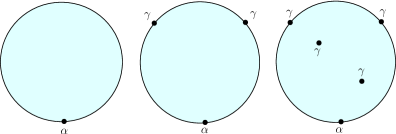
Figure 7. Left: $\mathrm{QD}_{0,1}(\gamma,\alpha)$ Middle: $\mathrm{QD}_{0,3}(\gamma,\alpha)$ Right: $\mathrm{QD}_{2,3}(\gamma,\alpha)$

More generally, for fixed $\ell_{1},\ldots,\ldots,\ell_{m}$, like in [AHS20, Section 2.6], we can define the measure $\mathrm{QD}_{1,m}(\gamma,\alpha)(\ell_{1},\ell_{2},\ldots,\ell_{m})$ using disintegration and it satisfies

(4.2.4) $$\mathrm{QD}_{1,m}(\gamma,\alpha)=\int_{0}^{\infty}\ldots\int_{0}^{\infty}\mathrm{QD}_{1,m}(\gamma,\alpha;\ell_{1},\ldots,\ell_{m})d\ell_{1}\ldots d\ell_{m}.$$

4.3. Conformal welding of thin and thick disks

Lemma 4.10.

For $W>\frac{\gamma^{2}}{2}$, let $\beta_{W}=\gamma+\frac{2-W}{\gamma}<Q$. Then we have

(4.3.1) $$\mathrm{QD}_{0,3}(\gamma,\beta_{W})=C\cdot\mathrm{QT}(2,2,W)$$

for some finite constant $C$.

Proof.

After applying [AHS21, Lemma 2.31] twice, we have

(4.3.2) $$\mathrm{LF}_{\mathbb{H}}^{(\beta_{W},0)}(d\phi)\nu_{\phi}(dx)\nu_{\phi}(dy)=\mathrm{LF}_{\mathbb{H}}^{(\beta_{W},0),(\gamma,x),(\gamma,y)}(d\phi)dxdy.$$

By disintegration, we can fix an embedding of $\mathrm{QD}_{0,3}(\gamma,\alpha)$ to be $(\mathbb{H},\phi,-1,0,1)$ so that $\phi$ has the law of $C\cdot\mathrm{LF}_{\mathbb{H}}^{(\beta_{W},0),(\gamma,-1),(\gamma,1)}$ for some finite constant $C$. Let $f:\mathbb{H}\to\mathcal{S}$ be the conformal map such that $f(-1)=-\infty,f(1)=\infty$ and $f(0)=0$. Therefore, by Definition 4.1, it has the law of $\mathrm{QT}(2,2,W)$ under push-forward of $f$. This completes the proof. ∎

Lemma 4.11.

Recall $\mathrm{LF}_{\mathbb{H}}^{(\beta_{i},z_{i})_{i}}$ from Definition 2.7. We have

(4.3.3) $$\mathrm{LF}_{\mathbb{H}}^{(\beta_{i},z_{i})_{i}}\left[f(\phi)\int_{\mathbb{H}}g(u)\mu_{\phi}(du)\right]=\mathrm{LF}_{\mathbb{H}}^{(\beta_{i},z_{i})_{i},(\gamma,u)}[f(\phi)]g(u)d^{2}u$$

for non-negative measurable functions $f$ and $g$.

Proof.

The proof is identical to that of [AHS21, Lemma 2.33] with $\widehat{\mathbb{C}}$ replaced by $\mathbb{H}$. ∎

Next we recall the decomposition theorem of thin quantum disk with one additional typical boundary marked point that is crucial to our derivation of the field law.

Lemma 4.12 ([AHS20, Proposition 4.4]).

For $W\in(0,\frac{\gamma^{2}}{2})$, we have

(4.3.4) $$\mathcal{M}^{\mathrm{disk}}_{2,\bullet}(W)=\left(1-\frac{2}{\gamma^{2}}W\right)^{2}\mathcal{M}^{\mathrm{disk}}_{0,2}(W)\times\mathcal{M}^{\mathrm{disk}}_{2,\bullet}(\gamma^{2}-W)\times\mathcal{M}^{\mathrm{disk}}_{0,2}(W).$$

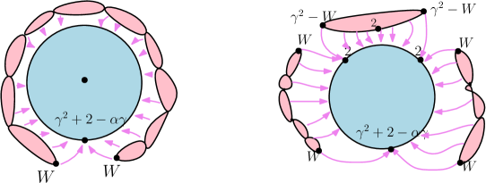
Figure 8. When $0<W<\frac{\gamma^{2}}{2}$, welding $\mathrm{QD}_{1,1}(\gamma,\alpha)$ with $\mathcal{M}^{\mathrm{disk}}_{0,2}(W)$ is equivalent to first welding $\mathrm{QD}_{0,3}(\gamma,\alpha)$ with three independent quantum disks $\mathcal{M}^{\mathrm{disk}}_{0,2}(W)$, $\mathcal{M}^{\mathrm{disk}}_{2,\bullet}(\gamma^{2}-W)$ and $\mathcal{M}^{\mathrm{disk}}_{0,2}(W)$ separately then de-weighting all the three additional boundary marked points and sampling an bulk marked point in the blue region according to quantum area measure.

Proposition 4.13.

Fix $0<\gamma<2$ and $0<W<\frac{\gamma^{2}}{2}$. For $\alpha\leq\gamma<Q$, let $W_{\alpha}=2-(\alpha-\gamma)\gamma\geq 2>\frac{\gamma^{2}}{2}$. Let $(\mathbb{H},\phi,\eta,0,i)$ be an embedding of

(4.3.5) $$\int_{0}^{\infty}\mathrm{QD}_{1,1}(\gamma,\alpha;\ell)\times\mathcal{M}_{0,2}^{\mathrm{disk}}(W;\ell)d\ell.$$

Then $\phi$ has the law of $C\cdot\mathrm{LF}_{\mathbb{H}}^{(\beta_{2W+W_{\alpha}},0),(\gamma,i)}$ for some finite constant $C$. Notice that $\alpha=\beta_{W_{\alpha}}=Q+\frac{\gamma}{2}-\frac{W_{\alpha}}{\gamma}$.

Proof.

Fix $0<W<\frac{\gamma^{2}}{2}$ and $\alpha\leq\gamma$. Start with the following four quantum surfaces:

(4.3.6) $$\mathrm{QD}_{0,3}(\gamma,\alpha),\mathcal{M}^{\mathrm{disk}}_{0,2}(W),\mathcal{M}^{\mathrm{disk}}_{0,2}(\gamma^{2}-W)\ \text{and}\ \mathcal{M}^{\mathrm{disk}}_{0,2}(W).$$

Notice that $\mathrm{QD}_{0,3}(\gamma,\alpha)$ has one $\alpha$ insertion and two $\gamma$ insertions along its boundary. First, weld two $\mathcal{M}^{\mathrm{disk}}_{0,2}(W)$ disks along the boundaries of $\mathrm{QD}_{0,3}(\gamma,\alpha)$ with $\gamma$ and $\alpha$ insertions, then weld $\mathcal{M}^{\mathrm{disk}}_{0,2}(\gamma^{2}-W)$ along the boundary of $\mathrm{QD}_{0,3}(\gamma,\alpha)$ with two $\gamma$ insertions. Precisely, we consider

(4.3.7) $$\begin{split}&\mathrm{Weld}\left(\mathrm{QD}_{0,3}(\gamma,\alpha),\mathcal{M}^{\mathrm{disk}}_{0,2}(W)\times\mathcal{M}^{\mathrm{disk}}_{0,2}(\gamma^{2}-W)\times\mathcal{M}^{\mathrm{disk}}_{0,2}(W)\right)\\ &:=\int_{0}^{\infty}\left(\iint_{0}^{\infty}\mathcal{M}^{\mathrm{disk}}_{0,2}(W;\ell_{1})\mathrm{QD}_{0,3}(\gamma,\alpha;\ell_{1},\ell_{2},\ell_{3})\mathcal{M}^{\mathrm{disk}}_{0,2}(W;\ell_{3})d\ell_{1}d\ell_{3}\right)\mathcal{M}^{\mathrm{disk}}_{0,2}(\gamma^{2}-W;\ell_{2})d\ell_{2}\\ &=\int_{0}^{\infty}\left(\iint_{0}^{\infty}\mathcal{M}^{\mathrm{disk}}_{0,2}(W;\ell_{1})\mathrm{QD}_{0,3}(\gamma,\alpha;\ell_{1},\ell_{2},\ell_{3})\mathcal{M}^{\mathrm{disk}}_{0,2}(W;\ell_{3})d\ell_{1}d\ell_{3}\right)\ell_{2}^{-1}\mathcal{M}^{\mathrm{disk}}_{2,\bullet}(\gamma^{2}-W;\ell_{2})d\ell_{2}\\ &=L_{2}^{-1}\cdot\mathrm{Weld}(\mathrm{QD}_{0,3}(\gamma,\alpha),\mathcal{M}^{\mathrm{disk}}_{0,2}(W)\times\mathcal{M}^{\mathrm{disk}}_{2,\bullet}(\gamma^{2}-W)\times\mathcal{M}^{\mathrm{disk}}_{0,2}(W))\\ &=\left(1-\frac{2}{\gamma^{2}}W\right)^{-2}\cdot L_{2}^{-1}\cdot\mathrm{Weld}\left(\mathrm{QD}_{0,3}(\gamma,\alpha),\mathcal{M}^{\mathrm{disk}}_{2,\bullet}(W)\right),\end{split}$$

where $L_{2}$ denotes the quantum length of welding interface between $\mathrm{QD}_{0,3}(\gamma,\alpha)$ and $\mathcal{M}^{\mathrm{disk}}_{0,2}(\gamma^{2}-W)$ and

(4.3.8) $$\mathrm{Weld}\left(\mathrm{QD}_{0,3}(\gamma,\alpha),\mathcal{M}^{\mathrm{disk}}_{2,\bullet}(W)\right):=\int_{0}^{\infty}\mathrm{QD}_{0,3}(\gamma,\alpha;\ell)\times\mathcal{M}^{\mathrm{disk}}_{2,\bullet}(W;\cdot,\ell)d\ell.$$

In (4.3.8), $\mathrm{QD}_{0,3}(\gamma,\alpha;\ell)$ represents the $\mathrm{QD}_{0,3}(\gamma,\alpha)$ conditioning on having total boundary length $\ell$ and $\mathcal{M}^{\mathrm{disk}}_{2,\bullet}(W;\cdot,\ell)$ represents the $\mathcal{M}^{\mathrm{disk}}_{2,\bullet}(W)$ conditioning on having left boundary length $\ell$. By de-weighting all the three marked points on the welding interface and sampling an additional bulk marked points in the inner region of (4.3.8), we have

(4.3.9) $$\begin{split}\mathrm{Weld}\left(\mathrm{QD}_{0,3}(\gamma,\alpha),\mathcal{M}^{\mathrm{disk}}_{2,\bullet}(W)\right)&=\int_{0}^{\infty}\mathrm{QD}_{0,3}(\gamma,\alpha;\ell)\times\mathcal{M}^{\mathrm{disk}}_{2,\bullet}(W;\ell)d\ell\\ &=\int_{0}^{\infty}\ell^{2}\cdot\mathrm{QD}_{0,1}(\gamma,\alpha;\ell)\times\mathcal{M}^{\mathrm{disk}}_{2,\bullet}(W;\ell)d\ell\\ &=\int_{0}^{\infty}\ell^{3}\cdot\mathrm{QD}_{0,1}(\gamma,\alpha;\ell)\times\mathcal{M}^{\mathrm{disk}}_{0,2}(W;\ell)d\ell\\ &=L_{T}^{3}\cdot\mathrm{Weld}(\mathrm{QD}_{0,1}(\gamma,\alpha),\mathcal{M}^{\mathrm{disk}}_{0,2}(W))\\ &=L_{T}^{3}\cdot A_{I}^{-1}\cdot\mathrm{Weld}(\mathrm{QD}_{1,1}(\gamma,\alpha),\mathcal{M}^{\mathrm{disk}}_{0,2}(W)),\end{split}$$

where $L_{T}$ denotes the quantum length of the total welding interface and $A_{I}$ denotes the quantum area of $\mathrm{QD}_{0,1}(\gamma,\alpha)$. Hence, by (4.3.7), (4.3.9), we have

(4.3.10) $$\begin{split}&\mathrm{Weld}\left(\mathrm{QD}_{0,3}(\gamma,\alpha),\mathcal{M}^{\mathrm{disk}}_{0,2}(W)\times\mathcal{M}^{\mathrm{disk}}_{0,2}(\gamma^{2}-W)\times\mathcal{M}^{\mathrm{disk}}_{0,2}(W)\right)\\ &=\left(1-\frac{2}{\gamma^{2}}W\right)^{-2}\cdot L_{2}^{-1}\cdot L_{T}^{3}\cdot A_{I}^{-1}\cdot\mathrm{Weld}(\mathrm{QD}_{1,1}(\gamma,\alpha),\mathcal{M}^{\mathrm{disk}}_{0,2}(W)).\end{split}$$

By applying Theorem 4.4 three times, we know that suppose $(\mathbb{H},\phi,\eta_{1},\eta_{2},\eta_{3},0,1,-1)$ is an embedding of

$$\mathrm{Weld}\left(\mathrm{QD}_{0,3}(\gamma,\alpha),\mathcal{M}^{\mathrm{disk}}_{0,2}(W)\times\mathcal{M}^{\mathrm{disk}}_{0,2}(\gamma^{2}-W)\times\mathcal{M}^{\mathrm{disk}}_{0,2}(W)\right),$$

then $\phi$ is independent of $(\eta_{1},\eta_{2},\eta_{3})$ and has the law of $C\cdot\mathrm{LF}_{\mathbb{H}}^{(\beta_{2W+W_{\alpha}},0),(0,-1),(0,1)}$ for some finite constant $C$. Here we emphasize the fact that weights of insertions $-1$ and $1$ are both zero due to the computation

$$\beta_{2+W+(\gamma^{2}-W)}=\beta_{2+\gamma^{2}}=0,$$

where the $2$ comes from the insertion $\gamma$ on $\mathrm{QD}_{0,3}(\gamma,\alpha)$, the $W$ comes from $\mathcal{M}^{\mathrm{disk}}_{0,2}(W)$ and the $\gamma^{2}-W$ comes from $\mathcal{M}_{0,2}^{\mathrm{disk}}(\gamma^{2}-W)$. Finally, by quantum surface relationship (4.3.10) and Lemma 4.11, we know that suppose $(\mathbb{H},\phi,0,i,\eta)$ is an embedding of $\mathrm{Weld}\left(\mathrm{QD}_{1,1}(\gamma,\alpha),\mathcal{M}^{\mathrm{disk}}_{0,2}(W)\right)$, then $\phi$ has the law of $C\cdot\mathrm{LF}_{\mathbb{H}}^{(\beta_{2W+W_{\alpha}},0),(\gamma,i)}$ for some finite constant $C$. ∎

4.4. Proof of Theorem 1.1

In this section, we prove Theorem 1.1 by inductively welding thin disks along the $\mathrm{QD}_{1,1}$.

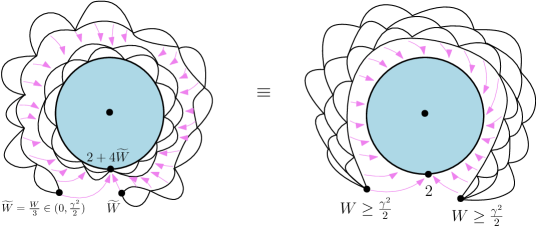
Figure 9. Illustration of the induction procedure in the proof of Theorem 1.1: suppose $W\geq\frac{\gamma^{2}}{2}$ and $\widetilde{W}=\frac{W}{3}\in(0,\frac{\gamma^{2}}{2})$, then welding a thick quantum disk $\mathcal{M}^{\mathrm{disk}}_{0,2}(W)$ is equivalent to welding three thin quantum disks $\mathcal{M}^{\mathrm{disk}}_{0,2}(\widetilde{W})$. Notice that here we only care about the law of the underlying random field.

Proof of Theorem 1.1.

By Proposition 3.1, we have the correct curve law and know that the curve law is independent of the underlying random field. Therefore, it remains to derive the field law. Fix $0<\gamma<2$ and $0<W<\frac{\gamma^{2}}{2}$. For $\alpha\leq\gamma$, let $W_{\alpha}=2-(\alpha-\gamma)\gamma\geq 2$. Let $(\mathbb{H},\phi,\eta,0,i)$ be an embedding of quantum surface

(4.4.1) $$\int_{0}^{\infty}\mathrm{QD}_{1,1}(\gamma,\alpha;\ell)\times\mathcal{M}_{0,2}^{\mathrm{disk}}(W;\ell)d\ell.$$

By Proposition 4.13, $\phi$ has the law of $C\cdot\mathrm{LF}_{\mathbb{H}}^{(\beta_{2W+W_{\alpha}},0),(\gamma,i)}$ for some finite constant $C$. Therefore, in order to prove the Theorem 1.1, we only need to extend the range of $W$ from $(0,\frac{\gamma^{2}}{2})$ to $(0,\infty)$. For any $W\geq\frac{\gamma^{2}}{2}$, there exists some integer $n\geq 2$ such that $\widetilde{W}=\frac{W}{n}\in(0,\frac{\gamma^{2}}{2})$. Moreover, by Theorem 2.22, we have

(4.4.2) $$\begin{split}&\int_{0}^{\infty}\mathrm{QD}_{1,1}(\ell)\times\mathcal{M}_{0,2}^{\mathrm{disk}}(W;\ell)d\ell\\ &=\int_{0}^{\infty}\mathrm{QD}_{1,1}(\ell)\underbrace{\mathcal{M}_{0,2}^{\mathrm{disk}}(\widetilde{W};\ell,\ell_{1})\mathcal{M}_{0,2}^{\mathrm{disk}}(\widetilde{W};\ell_{1},\ell_{2})\ldots\mathcal{M}_{0,2}^{\mathrm{disk}}(\widetilde{W};\ell_{n-2},\ell_{n-1})\mathcal{M}_{0,2}^{\mathrm{disk}}(\widetilde{W};\ell_{n-1},\ell_{n})}_{n\ \text{thin disks}}d\vec{\ell}\\ &=\int_{0}^{\infty}\left(\left(\left(\left(\mathrm{QD}_{1,1}(\ell)\mathcal{M}_{0,2}^{\mathrm{disk}}(\widetilde{W};\ell,\ell_{1})\right)\mathcal{M}_{0,2}^{\mathrm{disk}}(\widetilde{W};\ell_{1},\ell_{2})\right)\ldots\mathcal{M}_{0,2}^{\mathrm{disk}}(\widetilde{W};\ell_{n-2},\ell_{n-1})\right)\mathcal{M}_{0,2}^{\mathrm{disk}}(\widetilde{W};\ell_{n-1},\ell_{n})\right)d\vec{\ell},\end{split}$$

where $d\vec{\ell}=d\ell d\ell_{1},\ldots,d\ell_{n}$. Notice that $\mathrm{QD}_{1,1}=C\cdot\mathrm{QD}_{1,1}(\gamma,\gamma)$ by definition and $W_{\gamma}=2$. By applying Proposition 4.13 $n$ times from the inner bracket to outer bracket, we have that suppose $(\mathbb{H},\phi,\eta,0,i)$ is an embedding of $(\ref{4.4.1})$, then $\phi$ has the law of $C\cdot\mathrm{LF}_{\mathbb{H}}^{(\gamma,i),(\beta_{2+2n\widetilde{W}},0)}$, which is the same as $C\cdot\mathrm{LF}_{\mathbb{H}}^{(\gamma,i),(\beta_{2+2W},0)}$ for some finite constant $C$. This completes the proof. ∎

5. Proof of Theorem 1.3 via uniform embeddings of quantum surfaces

5.1. Uniform embedding of quantum surfaces

To start, recall that $\mathrm{conf}(\mathbb{H})$ is the group of conformal automorphisms of $\mathbb{H}$ where group multiplication $\cdot$ is the function composition $f\cdot g=f\circ g$. Let $\mathbf{m}_{\mathbb{H}}$ be a Haar measure on $\mathrm{conf}(\mathbb{H})$, which is both left and right invariant. Suppose $\mathfrak{f}$ is sampled from $\mathbf{m}_{\mathbb{H}}$ and $\phi\in H^{-1}(\mathbb{H})$, then we call the random function $\mathfrak{f}\bullet_{\gamma}\phi=\phi\circ\mathfrak{f}^{-1}+Q|\log(\mathfrak{f}^{-1})^{\prime}|$ the uniform embedding of $(\mathbb{H},\phi)$ via $\mathbf{m}_{\mathbb{H}}$. By invariance property of Haar measure, the law of $\mathfrak{f}\bullet_{\gamma}\phi$ only depends on $(\mathbb{H},\phi)$ as quantum surface. Let $(z_{i})_{1\leq i\leq n}\in\mathbb{H},(s_{j})_{1\leq j\leq m}\in\partial\mathbb{H}$ be groups of bulk and boundary marked points respectively. Suppose $(\mathbb{H},h,z_{1}\ldots,z_{n},s_{1},\ldots,s_{m})$ is a marked quantum surface, then we call $\mathbf{m}_{\mathbb{H}}\ltimes(\mathbb{H},h,z_{1}\ldots,z_{n},s_{1},\ldots,s_{m})$ the uniform embedding of $(\mathbb{H},h,z_{1}\ldots,z_{n},s_{1},\ldots,s_{m})$ via $\mathbf{m}_{\mathbb{H}}$.

Lemma 5.1 ([ARS22, Lemma $3.7$]).

Define three measures $A,N,K$ on the conformal automorphism group $\mathrm{conf}(\mathbb{H})$ on $\mathbb{H}$ as follows. Sample $\mathbf{t}$ from $1_{t>0}\frac{1}{t}dt$ and let $a:z\mapsto\mathbf{t}z$. Sample $\mathbf{s}$ from Lebesgue measure on $\mathbb{R}$ and let $n:z\mapsto z+\mathbf{s}$. Sample $\mathbf{u}$ from $\mathbbm{1}_{\{-\frac{\pi}{2}<u<\frac{\pi}{2}\}}du$ and let $k:z\mapsto\frac{z\cos\mathbf{u}-\sin\mathbf{u}}{z\sin\mathbf{u}+\cos\mathbf{u}}$. Let $A,N,K$ be the law of $a,n,k$ respectively, then the law of $a\circ n\circ k$ under $A\times N\times K$ is equal to $\mathbf{m}_{\mathbb{H}}$.

Lemma 5.2.

Suppose $\mathfrak{f}$ is sampled from $\mathbf{m}_{\mathbb{H}}$, then the joint law of $(\mathfrak{f}(0),\mathfrak{f}(i))$ is $\frac{1}{\Im q\cdot|p-q|^{2}}dpdq^{2}$.

Proof.

By the definition of $A,N$ and $K$ in Lemma 5.1, the $\mathfrak{f}(i)$ and $\mathfrak{f}(0)$ has the marginal law of $\mathbf{t}\mathbf{s}+\mathbf{t}i$ and $\mathbf{t}\tan\mathbf{u}+\mathbf{t}\mathbf{s}$ respectively, where $\mathbf{t}$ is sampled from $\mathbf{1}_{\{t>0\}}\frac{1}{t}dt,\mathbf{s}$ is sampled from $ds$, and $\mathbf{u}$ is sampled from $\mathbbm{1}_{\{-\frac{\pi}{2}<u<\frac{\pi}{2}\}}du$. Let $x=ts,y=t$ and $z=t\tan u+st$, then we have

$$\frac{1}{t}dsdtdu=\left(\frac{1}{y^{2}}dxdy\right)\left(\frac{y}{y^{2}+(z-x)^{2}}dz\right)=\frac{1}{\Im q\cdot|p-q|^{2}}dpd^{2}q.$$

Therefore the joint law of $(\mathfrak{f}(0),\mathfrak{f}(i))$ is equal to $\frac{1}{\Im q\cdot|p-q|^{2}}dpdq^{2}$. ∎

Lemma 5.3.

Let $f\in\mathrm{conf}(\mathbb{H})$ be such that $f(0)=p\in\mathbb{R}$ and $f(i)=q\in\mathbb{H}$, then we have that

(5.1.1) $$|f^{\prime}(i)|=\Im q\qquad\text{and}\qquad f^{\prime}(0)=\frac{|q-p|^{2}}{\Im q}.$$

Proof.

Write $f(z)=\frac{az+b}{cz+d}$ with $ad-bc=1$. Since $f(0)=p$ and $f(i)=q$, we have that

$$\begin{cases}\Re(q)&=\frac{ac+bd}{c^{2}+d^{2}},\\ \Im(q)&=\frac{1}{c^{2}+d^{2}},\\ p&=\frac{b}{d},\\ ad-bc&=1.\end{cases}$$

Furthermore, we have $|f^{\prime}(i)|=\frac{1}{c^{2}+d^{2}}$ and $f^{\prime}(0)=\frac{1}{d^{2}}$. Since $\frac{c^{2}}{d^{2}}=\frac{|\Re(q-p)|^{2}}{|\Im q|^{2}}$ and $c^{2}+d^{2}=\frac{1}{\Im q}$, $f^{\prime}(0)=\frac{|\Re(q-p)|^{2}}{\Im q}+\Im q=\frac{|q-p|^{2}}{\Im q}$ and $|f^{\prime}(i)|=\Im q$. This completes the proof. ∎

5.2. Proof of Theorem 1.3

Fix $p\in\mathbb{R}$ and $\gamma\in(0,2)$. Recall that for any $\eta\in\mathrm{Bubble}_{\mathbb{H}}(p)$, $D_{\eta}(p)$ denotes the component of $\mathbb{H}\backslash\eta$ which is encircled by $\eta$. Let $|D_{\eta}(p)|$ denote the euclidean area of $D_{\eta}(p)$. For $W>0$, let $\rho=W-2$. Define

(5.2.1) $$\begin{split}\widetilde{\mathrm{SLE}_{\kappa,p}^{\mathrm{bubble}}(\rho)}:=\frac{1}{|D_{\eta}(p)|}\int_{\mathbb{H}}|q-p|^{W-\frac{2W(W+2)}{\gamma^{2}}}\left(\Im q\right)^{\frac{W(W+2)}{\gamma^{2}}-\frac{W}{2}}\mathrm{SLE}_{\kappa,p}^{\mathrm{bubble}}(\rho)[d\eta|{q\in D_{\eta}(p)}]d^{2}q.\end{split}$$

Lemma 5.4.

For $W>0$, let $\beta_{2W+2}=\gamma-\frac{2W}{\gamma}$. There exists some constant $C\in(0,\infty)$ such that

(5.2.2) $$\mathbf{m}_{\mathbb{H}}\ltimes\left(\int_{0}^{\infty}\mathcal{M}^{\mathrm{disk}}_{0,2}(W;\cdot,\ell)\times\mathrm{QD}_{0,1}(\ell)d\ell\right)=C\cdot\mathrm{LF}_{\mathbb{H}}^{(\beta_{2W+2},p)}(d\phi)\times\widetilde{\mathrm{SLE}^{\mathrm{bubble}}_{\kappa,p}(\rho)(d\eta)}dp.$$

Furthermore, there exists some constant $C\in(0,\infty)$

(5.2.3) $$\mathbf{m}_{\mathbb{H},0}\ltimes\left(\int_{0}^{\infty}\mathcal{M}^{\mathrm{disk}}_{0,2}(W;\cdot,\ell)\times\mathrm{QD}_{0,1}(\ell)d\ell\right)=C\cdot\mathrm{LF}_{\mathbb{H}}^{(\beta_{2W+2},0)}(d\phi)\times\widetilde{\mathrm{SLE}^{\mathrm{bubble}}_{\kappa,0}(\rho)(d\eta)},$$

where recall that $\mathbf{m}_{\mathbb{H},0}$ is a Haar measure on $\mathrm{conf}(\mathbb{H},0)$, i.e., the group of conformal automorphisms of $\mathbb{H}$ fixing $0$.

Proof.

By Theorem 1.1, suppose $(\mathbb{H},\phi,\eta,0,i)$ is an embedding of quantum surface $\int_{0}^{\infty}\mathcal{M}^{\mathrm{disk}}_{0,2}(W;\cdot,\ell)\times\mathrm{QD}_{1,1}(\ell)d\ell$, then $(\phi,\eta)$ has the law of

(5.2.4) $$C\cdot\mathrm{LF}_{\mathbb{H}}^{(\gamma,i),\beta_{2W+2},0)}(d\phi)\times\mathrm{SLE}_{\kappa,0}^{\mathrm{bubble}}(\rho)[d\eta|{i\in D_{\eta}(0)}]$$

for some constant $C\in(0,\infty)$. By Proposition 2.12 and Lemma 5.3, for any $f\in\mathrm{conf}(\mathbb{H})$ with $f(0)=p\in\mathbb{R}$ and $f(i)=q\in\mathbb{H}$, we have

(5.2.5) $$\begin{split}f_{*}\mathrm{LF}_{\mathbb{H}}^{(\gamma,i),(\beta_{2W+2},0)}&=|f^{\prime}(0)|^{\Delta_{\beta_{2W+2}}}|f^{\prime}(i)|^{2\Delta_{\gamma}}\mathrm{LF}_{\mathbb{H}}^{(\gamma,q),(\beta_{2W+2},p)}\\ &=\left(\frac{|q-p|^{2}}{\Im q}\right)^{\Delta_{\beta_{2W+2}}}\cdot\left(\Im q\right)^{2\Delta_{\gamma}}\cdot\mathrm{LF}_{\mathbb{H}}^{(\gamma,q),(\beta_{2W+2},p)}.\end{split}$$

Recall that for $\alpha\in\mathbb{R}$, $\Delta_{\alpha}=\frac{\alpha}{2}(Q-\frac{\alpha}{2})$. By Lemma 5.2, if $f$ is sampled from a $\mathbf{m}_{\mathbb{H}}$, then the joint law of $(f(0),f(i))$ is $\frac{1}{\Im q\cdot|p-q|^{2}}dpdq^{2}$. Therefore, suppose $f$ is sampled from a $\mathbf{m}_{\mathbb{H}}$, then $f_{*}\mathrm{LF}_{\mathbb{H}}^{(\gamma,i),(\beta_{2W+2},0)}$ has the law of

(5.2.6) $$\begin{split}&\frac{1}{\Im q\cdot|p-q|^{2}}\cdot\left(\frac{|q-p|^{2}}{\Im q}\right)^{\Delta_{\beta_{2W+2}}}\cdot\left(\Im q\right)^{2\Delta_{\gamma}}\cdot\mathrm{LF}_{\mathbb{H}}^{(\gamma,q),(\beta_{2W+2},p)}dpdq^{2}\\ &=|q-p|^{W-\frac{2W(W+2)}{\gamma^{2}}}\left(\Im q\right)^{\frac{W(W+2)}{\gamma^{2}}-\frac{W}{2}}\mathrm{LF}_{\mathbb{H}}^{(\gamma,q),(\beta_{2W+2},p)}dpd^{2}q.\end{split}$$

Moreover, since $\mathrm{SLE}_{\kappa,0}^{\mathrm{bubble}}(\rho)[d\eta|{i\in D_{\eta}(0)}]$ is a probability measure, for fixed $f\in\mathrm{conf}(\mathbb{H})$ with $f(0)=p$ and $f(i)=q$, we have

(5.2.7) $$f_{*}\mathrm{SLE}_{\kappa,0}^{\mathrm{bubble}}(\rho)[d\eta|{i\in D_{\eta}(0)}]=\mathrm{SLE}_{\kappa,0}^{\mathrm{bubble}}(\rho)[d\eta|{q\in D_{\eta}(p)}].$$

Combining (5.2.4) ,(5.2.6) and (5.2.7), we have

(5.2.8) $$\begin{split}&\mathbf{m}_{\mathbb{H}}\ltimes\left(\int_{0}^{\infty}\mathcal{M}^{\mathrm{disk}}_{0,2}(W;\cdot,\ell)\times\mathrm{QD}_{1,1}(\ell)d\ell\right)\\ &=C\cdot|q-p|^{W-\frac{2W(W+2)}{\gamma^{2}}}\left(\Im q\right)^{\frac{W(W+2)}{\gamma^{2}}-\frac{W}{2}}\mathrm{LF}_{\mathbb{H}}^{(\gamma,q),(\beta_{2W+2},p)}\times\mathrm{SLE}_{\kappa,0}^{\mathrm{bubble}}(\rho)[d\eta|{q\in D_{\eta}(p)}]dpd^{2}q.\end{split}$$

On the other hand, by [AHS21, Lemma 2.32] (the proof is identical with the domain replaced by $\mathbb{H}$),

(5.2.9) $$\begin{split}&\mathrm{LF}_{\mathbb{H}}^{(\beta_{2W+2},p)}(d\phi)\times\widetilde{\mathrm{SLE}^{\mathrm{bubble}}_{\kappa,p}(\rho)(d\eta)}\mathbbm{1}_{D_{\eta}(p)}(\mu_{\phi}(d^{2}q))dp\\ &=\mathrm{LF}_{\mathbb{H}}^{(\beta_{2W+2},p),(\gamma,q)}(d\phi)\times\widetilde{\mathrm{SLE}_{\kappa,p}^{\mathrm{bubble}}(\rho)(d\eta)}\mathbbm{1}_{D_{\eta}(p)}(d^{2}q)dp\\ &=\mathrm{LF}_{\mathbb{H}}^{(\beta_{2W+2},p),(\gamma,q)}(d\phi)\cdot|q-p|^{W-\frac{2W(W+2)}{\gamma^{2}}}\left(\Im q\right)^{\frac{W(W+2)}{\gamma^{2}}-\frac{W}{2}}\mathrm{SLE}_{\kappa,p}^{\mathrm{bubble}}(\rho)[d\eta|{q\in D_{\eta}(p)}]d^{2}qdp.\end{split}$$

Hence, by (5.2.8) and (5.2.9), we have

(5.2.10) $$\begin{split}\mathbf{m}_{\mathbb{H}}\ltimes\left(\int_{0}^{\infty}\mathcal{M}^{\mathrm{disk}}_{0,2}(W;\cdot,\ell)\times\mathrm{QD}_{1,1}(\ell)d\ell\right)=C\cdot\mathrm{LF}_{\mathbb{H}}^{(\beta_{2W+2},p)}(d\phi)\times\widetilde{\mathrm{SLE}^{\mathrm{bubble}}_{\kappa,p}(\rho)(d\eta)}\mu_{\phi}(\mathbbm{1}_{D_{\eta}(p)}d^{2}q)dp\end{split}$$

for some constant $C\in(0,\infty)$. After de-weighting both sides of (5.2.10) by the quantum area of $D_{\eta}(p)$ and forgetting the bulk marked point, we have

(5.2.11) $$\mathbf{m}_{\mathbb{H}}\ltimes\left(\int_{0}^{\infty}\mathcal{M}^{\mathrm{disk}}_{0,2}(W;\cdot,\ell)\times\mathrm{QD}_{0,1}(\ell)d\ell\right)=C\cdot\mathrm{LF}_{\mathbb{H}}^{(\beta_{2W+2},p)}(d\phi)\times\widetilde{\mathrm{SLE}^{\mathrm{bubble}}_{\kappa,p}(\rho)(d\eta)}dp.$$

Furthermore, if we consider the $\mathbf{m}_{\mathbb{H},0}$, which is a Haar measure on the subgroup of $\mathrm{conf}(\mathbb{H})$ fixing $0$, i.e., $\mathrm{conf}(\mathbb{H},0)$, then we have

(5.2.12) $$\mathbf{m}_{\mathbb{H},0}\ltimes\left(\int_{0}^{\infty}\mathcal{M}^{\mathrm{disk}}_{0,2}(W;\cdot,\ell)\times\mathrm{QD}_{0,1}(\ell)d\ell\right)=C\cdot\mathrm{LF}_{\mathbb{H}}^{(\beta_{2W+2},0)}(d\phi)\times\widetilde{\mathrm{SLE}^{\mathrm{bubble}}_{\kappa,0}(\rho)(d\eta)}.$$

Note that equation (5.2.12) should be viewed as the disintegration of equation (5.2.11) over its boundary marked point. This finishes the proof. ∎

Lemma 5.5.

Fix $\rho>-2$. Then there exists some constant $C\in(0,\infty)$ such that

(5.2.13) $$\mathrm{SLE}^{\mathrm{bubble}}_{\kappa,0}(\rho)=C\cdot\widetilde{\mathrm{SLE}^{\mathrm{bubble}}_{\kappa,0}(\rho)},$$

where the constant $C$ equals to $\mathrm{SLE}^{\mathrm{bubble}}_{\kappa,0}(\rho)[i\in D_{\eta}(0)]$.

Proof.

Notice that

$$|D_{\eta}(0)|\cdot\mathrm{SLE}^{\mathrm{bubble}}_{\kappa,0}(\rho)(d\eta) =\int_{\mathbb{H}}\mathbbm{1}_{q\in D_{\eta}(0)}\mathrm{SLE}^{\mathrm{bubble}}_{\kappa,0}(\rho)(d\eta)d^{2}q$$

$$=\int_{\mathbb{H}}\mathrm{SLE}^{\mathrm{bubble}}_{\kappa,0}(\rho)[q\in D_{\eta}(0)]\cdot\mathrm{SLE}^{\mathrm{bubble}}_{\kappa,0}(\rho)[d\eta|q\in D_{\eta}(0)]d^{2}q.$$

Let $\psi\in\mathrm{conf}(\mathbb{H})$ be such that $\psi(i)=q$ and $\psi(0)=0$ and it is easy to show that $\psi^{\prime}(0)=\frac{|q|^{2}}{\Im q}$. By [Zha22, Theorem $3.16$], we have

(5.2.14) $$\mathrm{SLE}^{\mathrm{bubble}}_{\kappa,0}(\rho)[q\in D_{\eta}(0)]=\psi^{\prime}(0)^{-\alpha}\cdot\mathrm{SLE}^{\mathrm{bubble}}_{\kappa,0}(\rho)[i\in D_{\eta}(0)],$$

where $\alpha=\frac{(\rho+2)(2\rho+8-\kappa)}{2\kappa}$. Since $W=\rho+2$, we have

(5.2.15) $$\psi^{\prime}(0)^{-\alpha}=|q|^{W-\frac{2W(W+2)}{\kappa}}(\Im q)^{-\frac{W}{2}+\frac{W(W+2)}{\kappa}}.$$

Hence,

(5.2.16) $$\mathrm{SLE}^{\mathrm{bubble}}_{\kappa,0}(\rho)[q\in D_{\eta}(0)]=C\cdot|q|^{W-\frac{2W(W+2)}{\kappa}}(\Im q)^{-\frac{W}{2}+\frac{W(W+2)}{\kappa}},$$

where $C=\mathrm{SLE}^{\mathrm{bubble}}_{\kappa,0}(\rho)[i\in D_{\eta}(0)]\in(0,\infty)$ by Corollary 2.4. Therefore, by (5.2.1),

(5.2.17) $$\begin{split}\mathrm{SLE}^{\mathrm{bubble}}_{\kappa,0}(\rho)&=C\cdot\frac{1}{|D_{\eta}(0)|}\int_{\mathbb{H}}|q|^{W-\frac{2W(W+2)}{\kappa}}(\Im q)^{-\frac{W}{2}+\frac{W(W+2)}{\kappa}}\mathrm{SLE}^{\mathrm{bubble}}_{\kappa,0}(\rho)[d\eta|q\in D_{\eta}(0)]d^{2}q\\ &=C\cdot\widetilde{\mathrm{SLE}_{\kappa,0}^{\mathrm{bubble}}(\rho)}.\end{split}$$

This completes the proof. ∎

Corollary 5.6.

Fix $\rho>-2$ and $p\in\mathbb{R}$. Then there exists some constant $C\in(0,\infty)$ such that

(5.2.18) $$\mathrm{SLE}^{\mathrm{bubble}}_{\kappa,p}(\rho)=C\cdot\widetilde{\mathrm{SLE}^{\mathrm{bubble}}_{\kappa,p}(\rho)}.$$

Proof.

Fix $p\in\mathbb{R}$. Let $f_{p}\in\mathrm{conf}(\mathbb{H})$ be such that $f_{p}(z)=z+p$. Since $\mathrm{SLE}_{\kappa,0}^{\mathrm{bubble}}[d\eta|q\in D_{\eta}(0)]$ is a probability measure on $\mathrm{Bubble}_{\mathbb{H}}(0,q)$ for all $q$,

(5.2.19) $$f_{p}\left(\mathrm{SLE}_{\kappa,0}^{\mathrm{bubble}}[d\eta|q\in D_{\eta}(0)]\right)=\mathrm{SLE}_{\kappa,p}^{\mathrm{bubble}}[d\eta|q\in D_{\eta}(p)].$$

Hence,

(5.2.20) $$\begin{split}&f_{p}\left(\widetilde{\mathrm{SLE}_{\kappa,0}^{\mathrm{bubble}}(\rho)}\right)\\ &=f_{p}\left(\frac{1}{|D_{\eta}(0)|}\int_{\mathbb{H}}|q|^{W-\frac{2W(W+2)}{\kappa}}(\Im q)^{-\frac{W}{2}+\frac{W(W+2)}{\kappa}}\mathrm{SLE}^{\mathrm{bubble}}_{\kappa,0}(\rho)[d\eta|q\in D_{\eta}(0)]d^{2}q\right)\\ &=\frac{1}{|D_{\eta}(p)|}\int_{\mathbb{H}}|q-p|^{W-\frac{2W(W+2)}{\kappa}}(\Im(q-p))^{-\frac{W}{2}+\frac{W(W+2)}{\kappa}}\mathrm{SLE}^{\mathrm{bubble}}_{\kappa,p}(\rho)[d\eta|q\in D_{\eta}(p)]d^{2}q\\ &=\frac{1}{|D_{\eta}(p)|}\int_{\mathbb{H}}|q-p|^{W-\frac{2W(W+2)}{\kappa}}(\Im q)^{-\frac{W}{2}+\frac{W(W+2)}{\kappa}}\mathrm{SLE}^{\mathrm{bubble}}_{\kappa,p}(\rho)[d\eta|q\in D_{\eta}(p)]d^{2}q\\ &=\widetilde{\mathrm{SLE}_{\kappa,p}^{\mathrm{bubble}}(\rho)}.\end{split}$$

By Lemma 5.5, we have

(5.2.21) $$\mathrm{SLE}^{\mathrm{bubble}}_{\kappa,0}(\rho)=C\cdot\widetilde{\mathrm{SLE}^{\mathrm{bubble}}_{\kappa,0}.(\rho)}$$

The (5.2.18) follows from applying $f_{p}$ on both sides of (5.2.21). ∎

Proof of Theorem 1.3.

Theorem 1.3 follows immediately from Lemma 5.4, Lemma 5.5 and Corollary 5.6. ∎

6. SLE bubble zippers with a generic insertion

6.1. SLE bubble zippers with a generic bulk insertion

Definition 6.1 (Definition 2.9).

For $\alpha,\beta\in\mathbb{R}$, let $\phi$ be sampled from $\mathrm{LF}_{\mathbb{H}}^{(\alpha,i),(\beta,0)}$. We denote $\mathrm{QD}_{1,1}(\alpha,\beta)$ the infinite measure describing the law of quantum surface $(\mathbb{H},\phi,0,i)$.

Lemma 6.2.

Fix $\alpha,\beta\in\mathbb{R}$ and $q\in\mathbb{H}$, and we have

(6.1.1) $$\left(\Im q\right)^{2\Delta_{\alpha}-\Delta_{\beta}}|q|^{2\Delta_{\beta}}\mathrm{LF}_{\mathbb{H}}^{(\alpha,q)(\beta,0)}=(f_{\infty})_{*}\mathrm{LF}_{\mathbb{H}}^{(\beta,\infty),(\alpha,i)},$$

where $f_{\infty}\in\mathrm{conf}(\mathbb{H})$ is the conformal map with $f_{\infty}(\infty)=0$ and $f_{\infty}(i)=q$.

Proof.

For each $r>0$, let $f_{r}\in\mathrm{conf}(\mathbb{H})$ be a conformal map such that $f_{r}(r)=0$ and $f_{r}(i)=q$. By Proposition 2.12, we have

(6.1.2) $$\mathrm{LF}_{\mathbb{H}}^{(\beta,0),(\alpha,q)}=|f^{\prime}_{r}(i)|^{-2\Delta_{\alpha}}|f_{r}^{\prime}(r)|^{-\Delta_{\beta}}(f_{r})_{*}\mathrm{LF}_{\mathbb{H}}^{(\beta,r),(\alpha,i)}.$$

Assume $f_{r}(z)=\frac{a_{r}z+b_{r}}{c_{r}z+d_{r}}$, where $a_{r}d_{r}-b_{r}c_{r}=1$. Trivially, we have $|f_{r}^{\prime}(z)|=\frac{1}{(c_{r}z+d_{r})^{2}}$. Since $f_{r}(r)=0$ and $f_{r}(i)=q$, we have

$$\begin{cases}\Im q=\frac{1}{c_{r}^{2}+d_{r}^{2}},\\ \Re q=\frac{a_{r}c_{r}+b_{r}d_{r}}{c_{r}^{2}+d_{r}^{2}},\\ a_{r}r+b_{r}=0.\end{cases}$$

After solving the above equations, we have

$$\begin{cases}|f^{\prime}_{r}(r)|=a_{r}^{2}=\frac{|q|^{2}}{(r^{2}+1)\Im q},\\ |f_{r}^{\prime}(i)|=\Im q,\end{cases}\qquad\text{and}\qquad\begin{cases}a_{r}=\frac{|q|}{\sqrt{r^{2}+1}\sqrt{\Im q}},\\ b_{r}=-\frac{r|q|}{\sqrt{r^{2}+1}\sqrt{\Im q}},\\ c_{r}=\frac{\sqrt{|q|^{2}(r^{2}+1)-(\Im q-r\Re q)^{2}}}{\sqrt{r^{2}+1}\sqrt{\Im q}|q|},\\ d_{r}=\frac{\sqrt{\Im q}(1-r\frac{\Re q}{\Im q})}{\sqrt{r^{2}+1}|q|}.\end{cases}$$

After multiplying $r^{\beta(Q-\frac{\beta}{2})}$ on both sides of $(\ref{pr LCFT})$, we have

$$\left(\frac{r^{\beta(Q-\frac{\beta}{2})}}{(r^{2}+1)^{\frac{\beta}{2}(Q-\frac{\beta}{2})}}\right)(\Im q)^{2\Delta_{\alpha}-\Delta_{\beta}}|q|^{2\Delta_{\beta}}\mathrm{LF}_{\mathbb{H}}^{(\alpha,q),(\beta,0)}=r^{\beta(Q-\frac{\beta}{2})}(f_{r})_{*}\left[\mathrm{LF}_{\mathbb{H}}^{(\beta,r),(\alpha,i)}\right].$$

As $r\to\infty$, the left hand side becomes $(\Im q)^{2\Delta_{\alpha}-\Delta_{\beta}}|q|^{2\Delta_{\beta}}\mathrm{LF}_{\mathbb{H}}^{(\alpha,q),(\beta,0)}$. The right hand side converges in vague topology to $(f_{\infty})_{*}\mathrm{LF}_{\mathbb{H}}^{(\beta,\infty),(\alpha,i)}$ follows from the facts that $f_{r}\to f_{\infty}$ in the topology of uniform convergence of analytic function and its derivatives on all compact sets and [AHS21, Lemma $2.18$]. This completes the proof. ∎

Lemma 6.3.

Let $\alpha_{1},\alpha_{2},\beta\in\mathbb{R}$ and $\ell>0$. For $\varepsilon>0$, we define the measure $\mathrm{LF}_{\mathbb{H},\varepsilon}^{(\alpha_{2},i),(\beta,0)}$ through the Radon-Nikodym derivative as follows:

$$\frac{\mathrm{LF}_{\mathbb{H},\varepsilon}^{(\alpha_{2},i),(\beta,0)}(\ell)}{\mathrm{LF}_{\mathbb{H}}^{(\alpha_{1},i),(\beta,0)}(\ell)}(\phi):=\varepsilon^{\frac{1}{2}(\alpha_{2}^{2}-\alpha_{1}^{2})}e^{(\alpha_{2}-\alpha_{1})\phi_{\varepsilon}(i)}.$$

Furthermore, we have the weak convergence of measures

$$\lim_{\varepsilon\to 0}\mathrm{LF}_{\mathbb{H},\varepsilon}^{(\alpha_{2},i),(\beta,0)}(\ell)=\mathrm{LF}_{\mathbb{H}}^{(\alpha_{2},i),(\beta,0)}(\ell).$$

Proof.

We know that if $\phi$ is sampled from $\mathrm{LF}_{\mathbb{H}}^{(\alpha,i),(\beta,0)}(1)^{\#}$, then $\phi+\frac{2}{\gamma}\log\ell$ has the law of $\mathrm{LF}_{\mathbb{H}}^{(\alpha,i),(\beta,0)}(\ell)^{\#}$. Moreover, we have

$$\frac{|\mathrm{LF}_{\mathbb{H},\varepsilon}^{(\alpha,i),(\beta,0)}(\ell)|}{|\mathrm{LF}_{\mathbb{H},\varepsilon}^{(\alpha,i),(\beta,0)}(1)|}=\frac{|\mathrm{LF}_{\mathbb{H}}^{(\alpha,i),(\beta,0)}(\ell)|}{|\mathrm{LF}_{\mathbb{H}}^{(\alpha,i),(\beta,0)}(1)|}=\ell^{\frac{2}{\gamma}\left(\frac{\beta}{2}+\alpha-Q\right)-1}.$$

Let

$$\widetilde{h^{j}}=h-2Q\log|\cdot|_{+}+\alpha_{j}G_{\mathbb{H}}(\cdot,i)+\frac{\beta}{2}G_{\mathbb{H}}(\cdot,0),\qquad j=1,2$$

and $\widetilde{h^{2,\varepsilon}}=\widetilde{h^{1}}+(\alpha_{2}-\alpha_{1})G_{\mathbb{H},\varepsilon}(\cdot,i)$, where $G_{\mathbb{H},\varepsilon}(z,i)$ is the average of Green function $G_{\mathbb{H}}(z,\cdot)$ over $\partial B(i,\varepsilon)$. Notice that $\mathrm{Var}\left(h_{\varepsilon}(i)\right)=-\log\varepsilon-\log 2+o_{\varepsilon}(1)$ and $\mathbb{E}\left[e^{(\alpha_{2}-\alpha_{1})h_{\varepsilon}(i)}\right]=(1+o_{\varepsilon}(1))\left(2\varepsilon\right)^{-\frac{1}{2}(\alpha_{2}-\alpha_{1})^{2}}$. Furthermore, the average of $-2Q\log|\cdot|+\alpha G_{\mathbb{H}}(\cdot,i)+\frac{\beta}{2}G_{\mathbb{H}}(\cdot,0)$ over $\partial B(i,\varepsilon)$ is $-\alpha\log(2\varepsilon)+o_{\varepsilon}(1)$. Let $L_{1}=\nu_{\widetilde{h}^{1}}(\mathbb{R})$, $L_{2}=\nu_{\widetilde{h}^{2}}(\mathbb{R})$ and $L_{2,\varepsilon}=\nu_{\widetilde{h^{2,\varepsilon}}}(\mathbb{R})$. For any bounded continuous function $F$ on $H^{-1}(\mathbb{H})$, we have

$$\int\varepsilon^{\frac{1}{2}(\alpha_{2}^{2}-\alpha_{1}^{2})}e^{(\alpha_{2}-\alpha_{1})(\widetilde{h_{\varepsilon}^{1}}(i)-\frac{2}{\gamma}\log L_{1})}F(\widetilde{h^{1}}-\frac{2}{\gamma}\log L_{1})\cdot 2^{-\frac{\alpha_{1}^{2}}{2}}\cdot\frac{2}{\gamma}L_{1}^{-\frac{2}{\gamma}(\frac{\beta}{2}+\alpha_{1}-Q)}dh$$

$$=\int\frac{(1+o_{\varepsilon}(1))}{\mathbb{E}[e^{(\alpha_{2}-\alpha_{1})h_{\varepsilon}(i)}]}e^{(\alpha_{2}-\alpha_{1}){h_{\varepsilon}}(i)}F(\widetilde{h^{1}}-\frac{2}{\gamma}\log L_{1})\cdot 2^{-\frac{\alpha_{2}^{2}}{2}}\cdot\frac{2}{\gamma}L_{1}^{-\frac{2}{\gamma}(\frac{\beta}{2}+\alpha_{2}-Q)}dh$$

$$=\int(1+o_{\varepsilon}(1))F(\widetilde{h^{2,\varepsilon}}-\frac{2}{\gamma}\log L_{2,\varepsilon})\cdot 2^{-\frac{\alpha_{2}^{2}}{2}}\cdot\frac{2}{\gamma}L_{2,\varepsilon}^{-\frac{2}{\gamma}(\frac{\beta}{2}+\alpha_{2}-Q)}dh$$

$$\xrightarrow{\varepsilon\to 0}\int F(\widetilde{h^{2}}-\frac{2}{\gamma}\log L_{2})\cdot 2^{-\frac{\alpha_{2}^{2}}{2}}\cdot\frac{2}{\gamma}L_{2}^{-\frac{2}{\gamma}(\frac{\beta}{2}+\alpha_{2}-Q)}dh.$$

The second equality follows from the Girsanov’s Theorem. Since $L_{2}=(1+o_{\varepsilon}(1))L_{2,\varepsilon}$ and $\sup_{x\in\mathbb{R}}|G_{\mathbb{H}}(x,i)-G_{\mathbb{H},\varepsilon}(x,i)|=o_{\varepsilon}(1)$, the final $\varepsilon$ limit follows from the the Dominated Convergence Theorem. ∎

6.2. Proof of Theorem 1.5

Proof of Theorem 1.5.

By Theorem 1.1, we have

$$\mathrm{LF}_{\mathbb{H}}^{(\beta_{2W+2},0),(\gamma,i)}(1)\times\mathbf{m}=C_{W}\cdot\int_{0}^{\infty}\mathrm{QD}_{1,1}(\ell)\times\mathcal{M}^{\mathrm{disk}}_{0,2}(W;1,\ell)d\ell.$$

Let $(Y,\eta)$ be sampled from the left hand side. Let $\psi_{\eta}:\mathbb{H}\to D_{\eta}(i)$ be the conformal map fixing $0$ and $i$ and $\xi_{\eta}:\mathbb{H}\to D_{\eta}(\infty)$ be such that $\xi_{\eta}(0)=0^{-}$, $\xi_{\eta}(1)=0^{+}$ and $\xi_{\eta}(\infty)=\infty$. Let $X,Z\in H^{-1}(\mathbb{H})$ be such that

$$X=Y\circ\psi_{\eta}+Q\log|\psi_{\eta}^{\prime}|\qquad\text{and}\qquad Z=Y\circ\xi_{\eta}+Q\log|\xi_{\eta}^{\prime}|.$$

Notice that $\mathrm{QD}_{1,1}(\ell)$ embedded in $(\mathbb{H},0,i)$ has the law of $C\cdot\mathrm{LF}_{\mathbb{H}}^{(\gamma,i),(\gamma,0)}(r)$. Therefore, the $X$ has the law of

$$C_{W}\int_{0}^{\infty}|\mathcal{M}^{\mathrm{disk}}_{0,2}(W;1,\ell)|\cdot\mathrm{LF}_{\mathbb{H}}^{(\gamma,i),(\gamma,0)}(\ell)d\ell.$$

The conditional law of marked quantum surface $(\mathbb{H},Z,0,1)$ given $X$ is $\mathcal{M}^{\mathrm{disk}}_{0,2}(\beta_{W};1,\nu_{X}(\mathbb{R}))^{\#}$. Next, if we re-weight $X$ by $\varepsilon^{\frac{1}{2}(\alpha^{2}-\gamma^{2})}e^{(\alpha-\gamma)X_{\varepsilon}(i)}$ and send $\varepsilon$ to $0$, the law of $X$ converges weakly to

$$C_{W}\int_{0}^{\infty}|\mathcal{M}^{\mathrm{disk}}_{0,2}(W;1,\ell)|\cdot\mathrm{LF}_{\mathbb{H}}^{(\alpha,i),(\gamma,0)}(\ell)d\ell.$$

Consequently, the law of $Z$ conditioned on re-weighted $X$ is $\mathcal{M}^{\mathrm{disk}}_{0,2}(W;1,\nu_{X}(\mathbb{R}))^{\#}$.

Next, let $\theta_{i,\varepsilon}$ be the uniform probability measure on $\partial B(i,\varepsilon)$ for sufficiently small $\varepsilon$. Let $\theta^{\eta}_{i,\varepsilon}=(\psi_{\eta})_{*}(\theta_{i,\varepsilon})$ be the push-forward of $\theta_{i,\varepsilon}$ under $\psi_{\eta}$. Since $\psi^{\prime}_{\eta}$ is holomorphic and $\log|\psi^{\prime}_{\eta}|$ is harmonic,

$$X_{\varepsilon}(i)=(X,\theta_{i,\varepsilon})=(Y\circ\psi_{\eta}+Q\log|\psi_{\eta}^{\prime}|,\theta^{\eta}_{i,\varepsilon})=(Y,\theta^{\eta}_{i,|\psi^{\prime}_{\eta}(i)|\varepsilon})+Q\log|\psi^{\prime}_{\eta}(i)|.$$

Therefore, re-weighting by $\varepsilon^{\frac{1}{2}(\alpha^{2}-\gamma^{2})}e^{(\alpha-\gamma)X_{\varepsilon}(i)}$ is equivalent to re-weighting by

$$\varepsilon^{\frac{1}{2}(\alpha^{2}-\gamma^{2})}e^{(\alpha-\gamma)[(Y,\theta^{\eta}_{i,|\psi^{\prime}_{\eta}(i)|\varepsilon})+Q\log|\psi^{\prime}_{\eta}(i)|]}$$

$$=\left(\varepsilon|\psi_{\eta}^{\prime}(i)|\right)^{\frac{1}{2}(\alpha^{2}-\gamma^{2})}e^{(\alpha-\gamma)(Y,\theta^{\eta}_{i,|\psi^{\prime}_{\eta}(i)|\varepsilon})}|\psi_{\eta}^{\prime}(i)|^{-\frac{1}{2}\alpha^{2}+Q\alpha-2}.$$

Hence, we conclude that for any bounded continuous $F$ on $H^{-1}(\mathbb{H})^{3}$ and bounded continuous function $g$ on $\mathrm{Bubble}_{\mathbb{H}}(0,i)$ equipped with Hausdorff topology,

$$\lim_{\varepsilon\to 0}\int\int C_{W}\left(\varepsilon|\psi_{\eta}^{\prime}(i)|\right)^{\frac{1}{2}(\alpha^{2}-\gamma^{2})}e^{(\alpha-\gamma)(Y,\theta^{\eta}_{i,|\psi^{\prime}_{\eta}(i)|\varepsilon})}F(X,Y,Z)\mathrm{LF}_{\mathbb{H}}^{(\beta_{2W+2},0),(\gamma,i)}(1)(dY)g(\eta)\mathbf{m}_{\alpha}(d\eta)$$

$$=\int\int C_{W}F(\widetilde{X},\widetilde{Y},\widetilde{Z})\mathrm{LF}_{\mathbb{H}}^{(\beta_{2W+2},0),(\gamma,i)}(1)(d\widetilde{Y})g(\widetilde{\eta})\mathbf{m}_{\alpha}(d\widetilde{\eta}).$$

By conformal welding, $(X,Z)$ is uniquely determined by $(Y,\eta)$. Similarly, $(\widetilde{Y},\widetilde{\eta})$ is uniquely determined by $(\widetilde{X},\widetilde{Z})$. Therefore, when $(\widetilde{Y},\widetilde{\eta})$ is sampled from $\mathrm{LF}_{\mathbb{H}}^{(\beta_{2W+2},0),(\gamma,i)}\times\mathbf{m}_{\alpha}$, $\widetilde{X}$ has the law of

$$C_{W}\cdot\int_{0}^{\infty}|\mathcal{M}^{\mathrm{disk}}_{0,2}(W;1,\ell)|\cdot\mathrm{LF}_{\mathbb{H}}^{(\alpha,i),(\gamma,0)}(\ell)d\ell$$

and the conditional law of marked quantum surface $(\mathbb{H},\widetilde{Z},0,i)$ given $\widetilde{X}$ is $\mathcal{M}^{\mathrm{disk}}_{0,2}(W;1,\nu_{\widetilde{X}}(\mathbb{R}))$. This finishes the proof. ∎

7. Applications

7.1. Preliminary results on integrabilities of the LCFT

First, we recall the double gamma function $\Gamma_{b}(z)$. For $b$ such that $\Re(b)>0$, the $\Gamma_{b}(z)$ is a meromorphic function on $\mathbb{C}$ such that

$$\ln\Gamma_{b}(z)=\int_{0}^{\infty}\frac{1}{t}\left(\frac{e^{-zt}-e^{-(b+\frac{1}{b})t/2}}{(1-e^{-bt})(1-e^{-\frac{1}{b}t})}-\frac{\left(\frac{1}{2}(b+\frac{1}{b})-z\right)^{2}}{2}e^{-t}+\frac{z-\frac{1}{2}(b+\frac{1}{b})}{t}\right)dt$$

for $\Re(z)>0$ and it satisfies the following two shift equations:

(7.1.1) $$\frac{\Gamma_{b}(z)}{\Gamma_{b}(z+b)}=\frac{1}{\sqrt{2\pi}}\Gamma(bz)b^{-bz+\frac{1}{2}}\qquad\text{and}\qquad\frac{\Gamma_{b}(z)}{\Gamma_{b}(z+\frac{1}{b})}=\frac{1}{\sqrt{2\pi}}\Gamma\left(\frac{1}{b}z\right)\left(\frac{1}{b}\right)^{-\frac{1}{b}z+\frac{1}{2}}.$$

The above two shift equations allow us to extend $\Gamma_{b}(z)$ meromorphically from $\Re(z)>0$ to the entire complex plane $\mathbb{C}$. It has simple poles at $-nb-m\frac{1}{b}$ for nonnegative integers $m,n$. The double sine function is defined as

(7.1.2) $$S_{b}(z):=\frac{\Gamma_{b}(z)}{\Gamma_{b}(b+\frac{1}{b}-z)}.$$

We can now define the Liouville reflection coefficient $R$. For fixed $\mu_{1},\mu_{2}>0$, let $\sigma_{j}\in\mathbb{C}$ satisfy $\mu_{j}=e^{i\pi\gamma(\sigma_{j}-\frac{Q}{2})}$ and $\Re\sigma_{j}=\frac{Q}{2}$ for $j=1,2$ and define the following two meromorphic functions for $\beta\in\mathbb{C}$ as belows:

(7.1.3) $$\overline{R}(\beta,\mu_{1},\mu_{2}) =\frac{(2\pi)^{\frac{2}{\gamma}(Q-\beta)-\frac{1}{2}}(\frac{2}{\gamma})^{\frac{\gamma}{2}(Q-\beta)-\frac{1}{2}}}{(Q-\beta)\Gamma(1-\frac{\gamma^{2}}{4})^{\frac{2}{\gamma}(Q-\beta)}}\frac{\Gamma_{\frac{\gamma}{2}}(\beta-\frac{\gamma}{2})e^{i\pi(\sigma_{1}+\sigma_{2}-Q)(Q-\beta)}}{\Gamma_{\frac{\gamma}{2}}(Q-\beta)S_{\frac{\gamma}{2}}(\frac{\beta}{2}+\sigma_{2}-\sigma_{1})S_{\frac{\gamma}{2}}(\frac{\beta}{2}+\sigma_{1}-\sigma_{2})},$$

(7.1.4) $$R(\beta,\mu_{1},\mu_{2}) =-\Gamma\left(1-\frac{2}{\gamma}(Q-\beta)\right)\overline{R}(\beta,\mu_{1},\mu_{2}).$$

Proposition 7.1 ([RZ22, Theorem $1.7$]).

Let $\beta_{W}=Q=\frac{\gamma}{2}-\frac{W}{\gamma}\in(\frac{\gamma}{2},Q)$. Let $\mu_{1},\mu_{2}\geq 0$ not both be zero. Recall random field $\widehat{h}$ defined in Definition 2.15 of $\mathcal{M}^{\mathrm{disk}}_{0,2}(W)$. We have that

(7.1.5) $$\mathbb{E}\left[\left(\mu_{1}\nu_{\widehat{h}}(\mathbb{R})+\mu_{2}\nu_{\widehat{h}}(\mathbb{R}+\pi i)\right)^{\frac{2}{\gamma}(Q-\beta_{W})}\right]=\overline{R}(\beta_{W},\mu_{1},\mu_{2}).$$

Lemma 7.2 ([AHS21, Lemma $3.3$]).

For $W\in[\frac{\gamma^{2}}{2},\gamma Q)$ and $\beta_{W}=Q+\frac{\gamma}{2}-\frac{W}{\gamma}$, let $L_{1},L_{2}$ denote the left and right boundary length of weight $W$ quantum disk $\mathcal{M}^{\mathrm{disk}}_{0,2}(W)$, then the law of $\mu_{1}L_{1}+\mu_{2}L_{2}$ is

$$\mathbbm{1}_{\ell>0}\overline{R}(\beta_{W},\mu_{1},\mu_{2})\ell^{-\frac{2}{\gamma^{2}}W}d\ell.$$

Let $W=2,\mu_{1}=\mu_{2}=1$ and by independent sampling property of $\mathcal{M}^{\mathrm{disk}}_{0,2}(2)$, we have the following results on the joint law of left and right boundary length.

Proposition 7.3 ([DMS20], Proposition $5.1$).

For $\ell,\gamma>0$, we have

(7.1.6) $$|\mathcal{M}^{\mathrm{disk}}_{0,2}(2;\ell,r)|=\frac{(2\pi)^{\frac{4}{\gamma^{2}}-1}}{(1-\frac{\gamma^{2}}{4})\Gamma(1-\frac{\gamma^{2}}{4})^{\frac{4}{\gamma^{2}}}}(\ell+r)^{-\frac{4}{\gamma^{2}}-1}.$$

Proposition 7.4 ([AHS21, Proposition $3.6$]).

For $W\in(0,\frac{\gamma^{2}}{2})$ and $\beta_{W}=Q+\frac{\gamma}{2}-\frac{W}{\gamma}\in(Q,Q+\frac{\gamma}{2})$. Let $L_{W}$ and $R_{W}$ be the left and right quantum boundary lengths of weight-$W$ thin quantum disk $\mathcal{M}^{\mathrm{disk}}_{0,2}(W)$, and we have

(7.1.7) $$\mathcal{M}_{0,2}^{\mathrm{disk}}(W)\left[e^{-\mu_{1}L_{W}-\mu_{2}R_{W}}\right]=-\frac{\gamma}{2(\beta_{W}-Q)}R(\beta_{W};\mu_{1},\mu_{2}).$$

Next, we recall the two-pointed correlation function of the Liouville theory on $\mathbb{H}$ that was introduced in Section 1.2.2 when $\mu=0,\mu_{\partial}>0$. For bulk insertions $z_{i}$ with weights $\alpha_{i}$ and boundary insertions $s_{j}$ with weights $\beta_{j}$, the correlation function of LCFT at these points is defined using the following formal path integral:

(7.1.8) $$\left\langle\prod_{i=1}^{N}e^{\alpha_{i}\phi(z_{i})}\prod_{j=1}^{M}e^{\frac{\beta_{j}}{2}\phi(s_{j})}\right\rangle_{\mu_{\partial}}=\int_{X:\mathbb{H}\to\mathbb{R}}DX\prod_{i=1}^{N}e^{\alpha_{i}X(z_{i})}\prod_{j=1}^{M}e^{\frac{\beta_{j}}{2}X(s_{j})}e^{-S_{\mu_{\partial}}^{L}(X)}.$$

In the above formula, $DX$ is the formal uniform measure on infinite dimensional function space and $S^{\mu_{\partial}}_{L}(X)$ is the Liouville action functional given by

(7.1.9) $$S_{\mu_{\partial}}^{L}(X):=\frac{1}{4\pi}\int_{\mathbb{H}}\left(|\nabla_{g}X|^{2}+QR_{g}X\right)d\lambda_{g}+\frac{1}{2\pi}\int_{\mathbb{R}}\left(QK_{g}X+2\pi\mu_{\partial}e^{\frac{\gamma}{2}X}\right)d\lambda_{\partial g}.$$

For background Riemannian metric $g$ on $\mathbb{H}$, $\nabla_{g},R_{g},K_{g},d\lambda_{g},d\lambda_{\partial g}$ stand for the gradient, Ricci curvature, Geodesic curvature, volume form and line segment respectively. The subscript $\mu_{\partial}$ emphases the fact that we are considering the case when $\mu=0,\mu_{\partial}>0$. For $z\in\mathbb{H}$ and $s\in\mathbb{R}$, the bulk-boundary correlator is

(7.1.10) $$\left\langle e^{\alpha\phi(z)}e^{\frac{\beta}{2}\phi(s)}\right\rangle_{\mu_{\partial}}=\frac{G(\alpha,\beta)}{|z-\overline{z}|^{2\Delta_{\alpha}-\Delta_{\beta}}|z-s|^{2\Delta_{\beta}}}.$$

Next, we introduce the rigorous mathematical definition of $G(\alpha,\beta)$.

Definition 7.5 ([RZ22, Definition $1.5$]).

The function $G(\alpha,\beta)=\frac{2}{\gamma}\Gamma\left(\frac{2\alpha+\beta-2Q}{\gamma}\right)\left(\mu_{B}^{\frac{2Q-2\alpha-\beta}{\gamma}}\right)\overline{G}(\alpha,\beta)$, where for $\beta<Q$ and $\frac{\gamma}{2}-\alpha<\frac{\beta}{2}<\alpha$:

(7.1.11) $$\overline{G}(\alpha,\beta)=\mathbb{E}\left[\left(\int_{\mathbb{R}}\frac{g(x)^{\frac{\gamma}{4}(\frac{2}{\gamma}-\alpha-\frac{\beta}{2})}}{|x-i|^{\gamma\alpha}}e^{\frac{\gamma}{2}h(x)}dx\right)^{\frac{2}{\gamma}(Q-\alpha-\frac{\beta}{2})}\right].$$

In the above formula, $g(x)=\frac{1}{|x|_{+}^{4}},|x|_{+}=\max(|x|,1)$ and $h(x)$ is sampled from $P_{\mathbb{H}}$.

Theorem 7.6 ([RZ22, Theorem $1.7$]).

For $\gamma\in(0,2),\beta<Q$ and $\frac{\gamma}{2}-\alpha<\frac{\beta}{2}<\alpha$,

(7.1.12) $$\overline{G}(\alpha,\beta)=\left(\frac{2^{\frac{\gamma}{2}(\frac{\beta}{2}-\alpha)}2\pi}{\Gamma(1-\frac{\gamma^{2}}{4})}\right)^{\frac{2}{\gamma}(Q-\alpha-\frac{\beta}{2})}\frac{\Gamma(\frac{\gamma\alpha}{2}+\frac{\gamma\beta}{4}-\frac{\gamma^{2}}{4})\Gamma_{\frac{\gamma}{2}}(\alpha-\frac{\beta}{2})\Gamma_{\frac{\gamma}{2}}(\alpha+\frac{\beta}{2})\Gamma_{\frac{\gamma}{2}}(Q-\frac{\beta}{2})^{2}}{\Gamma_{\frac{\gamma}{2}}(Q-\frac{\beta}{2})\Gamma_{\frac{\gamma}{2}}(\alpha)^{2}\Gamma_{\frac{\gamma}{2}}(Q)}.$$

Lemma 7.7.

Fix $\ell>0$. Let $\gamma,\beta,\alpha$ be such that $\gamma\in(0,2),\beta<Q,\frac{\gamma}{2}-\alpha<\frac{\beta}{2}<\alpha$. Let $h$ be sampled from $P_{\mathbb{H}}$ and let $h_{\infty}(z)=h(z)+(\beta-2Q)\log|z|_{+}+\alpha G_{\mathbb{H}}(z,i)$. Let $\phi$ be sampled from $\mathrm{LF}_{\mathbb{H}}^{(\beta,\infty),(\alpha,i)}(d\phi)$ and for each bounded non-negative measurable function $f$ on $(0,\infty)$, we have

$$\mathrm{LF}_{\mathbb{H}}^{(\beta,\infty),(\alpha,i)}[f(\nu_{\phi}(\mathbb{R}))]=\int_{0}^{\infty}f(\ell)2^{-\frac{\alpha^{2}}{2}}\ell^{\frac{2}{\gamma}(\frac{1}{2}\beta+\alpha-Q)-1}\cdot\frac{2}{\gamma}\cdot\overline{G}(\alpha,\beta)d\ell,$$

where $\overline{G}(\alpha,\beta)$ is the two point (one bulk, one boundary) correlation function of Liouville theory on $\mathbb{H}$.

Proof.

It suffices to consider the case when $f(\ell)=\mathbbm{1}_{a<\ell<b}(\ell)$. By direct computation,

$$\mathrm{LF}_{\mathbb{H}}^{(\beta,\infty),(\alpha,i)}[f(\nu_{\phi}(\mathbb{R}))] =\mathbb{E}\left[\int_{\mathbb{R}}\mathbbm{1}_{\{e^{\frac{\gamma}{2}c}\nu_{h_{\infty}(\mathbb{R})}\in(a,b)\}}2^{-\frac{\alpha^{2}}{2}}e^{(\frac{1}{2}\beta+\alpha-Q)c}dc\right]$$

$$=\mathbb{E}\left[\int_{a}^{b}\nu_{h_{\infty}}(\mathbb{R})^{\frac{2}{\gamma}(Q-\alpha-\frac{1}{2}\beta)}2^{-\frac{\alpha^{2}}{2}}\ell^{\frac{2}{\gamma}(\frac{1}{2}\beta+\alpha-Q)-1}\cdot\frac{2}{\gamma}d\ell\right]$$

$$=\int_{a}^{b}2^{-\frac{\alpha^{2}}{2}}\ell^{\frac{2}{\gamma}(\frac{1}{2}\beta+\alpha-Q)-1}\cdot\frac{2}{\gamma}\cdot\mathbb{E}\left[\nu_{h_{\infty}(\mathbb{R})}^{\frac{2}{\gamma}(Q-\alpha-\frac{1}{2}\beta)}\right]d\ell.$$

The second line follows from the change of variable $\ell=e^{\frac{\gamma}{2}c}\nu_{h_{\infty}}(\mathbb{R})$. The third line follows from the finiteness of $\mathbb{E}\left[\nu_{h_{\infty}(\mathbb{R})}^{\frac{2}{\gamma}(Q-\alpha-\frac{1}{2}\beta)}\right]$ and Fubini’s theorem. The finiteness of $\mathbb{E}\left[\nu_{h_{\infty}(\mathbb{R})}^{\frac{2}{\gamma}(Q-\alpha-\frac{1}{2}\beta)}\right]$ is proved in [RZ22, Proposition $5.1$]. Furthermore,

$$\mathbb{E}\left[\nu_{h_{\infty}(\mathbb{R})}^{\frac{2}{\gamma}(Q-\alpha-\frac{1}{2}\beta)}\right] =\lim_{\varepsilon\downarrow 0}\mathbb{E}\left[\left(\int_{\mathbb{R}}\varepsilon^{\frac{\gamma^{2}}{4}}e^{\frac{\gamma}{2}h_{\varepsilon}(x)}e^{\frac{\gamma}{2}[(\beta-\frac{4}{\gamma})\log|x|_{+}+\alpha\widetilde{G}_{\mathbb{H}}(x,i)]}dx\right)^{\frac{2}{\gamma}(Q-\alpha-\frac{1}{2}\beta)}\right]$$

$$=\lim_{\varepsilon\downarrow 0}\mathbb{E}\left[\left(\int_{\mathbb{R}}e^{\frac{\gamma}{2}h_{\varepsilon}(x)-\frac{\gamma^{2}}{2}\mathbb{E}[h_{\varepsilon}(x)^{2}]}\frac{|x|_{+}^{\gamma\alpha+\frac{\gamma\beta}{2}-2}}{|x-i|^{\gamma\alpha}}dx\right)^{\frac{2}{\gamma}(Q-\alpha-\frac{1}{2}\beta)}\right]$$

$$=\mathbb{E}\left[\left(\int_{\mathbb{R}}e^{\frac{\gamma}{2}h_{\varepsilon}(x)-\frac{\gamma^{2}}{2}\mathbb{E}[h_{\varepsilon}(x)^{2}]}\frac{|x|_{+}^{\gamma\alpha+\frac{\gamma\beta}{2}-2}}{|x-i|^{\gamma\alpha}}dx\right)^{\frac{2}{\gamma}(Q-\alpha-\frac{1}{2}\beta)}\right]$$

$$=\mathbb{E}\left[\left(\int_{\mathbb{R}}e^{\frac{\gamma}{2}h(x)}\frac{|x|_{+}^{\gamma\alpha+\frac{\gamma\beta}{2}-2}}{|x-i|^{\gamma\alpha}}dx\right)^{\frac{2}{\gamma}(Q-\alpha-\frac{1}{2}\beta)}\right]$$

$$=\overline{G}(\alpha,\beta).$$

This completes the proof. ∎

7.2. Moments of the conformal radius of $\mathrm{SLE}_{\kappa}(\rho)$ bubbles

By (1.2.2) in Theorem 1.5,

(7.2.1) $$\mathrm{LF}_{\mathbb{H}}^{(\beta_{2W+2},0),(\alpha,i)}(1)\times\mathbf{m}_{\alpha}=C_{W}\cdot\int_{0}^{\infty}\mathrm{QD}_{1,1}(\alpha,\gamma;\ell)\times\mathcal{M}^{\mathrm{disk}}_{0,2}(W;1,\ell)d\ell$$

for $W>0$ and $\alpha\in\mathbb{R}$. By definition of $\mathbf{m}_{\alpha}$ (1.2.1),

(7.2.2) $$|\mathbf{m}_{\alpha}|=\mathbb{E}\left[|\psi^{\prime}_{\eta}(i)|^{2\Delta_{\alpha}-2}\right]$$

since $\mathbf{m}$ is a probability measure. Therefore, taking mass on both sides of (7.2.1) yields

(7.2.3) $$\left|\mathrm{LF}_{\mathbb{H}}^{(\beta_{2W+2},0),(\alpha,i)}(1)\right|\cdot\mathbb{E}\left[|\psi^{\prime}_{\eta}(i)|^{2\Delta_{\alpha}-2}\right]=C_{W}\cdot\int_{0}^{\infty}\left|\mathrm{QD}_{1,1}(\alpha,\gamma;\ell)\right|\left|\mathcal{M}^{\mathrm{disk}}_{0,2}(W;1,\ell)\right|d\ell.$$

Lemma 7.8.

Fix $\ell>0$ and $q\in\mathbb{H}$. Let $\gamma,\beta,\alpha$ be such that $\gamma\in(0,2),\beta<Q$ and $\frac{\gamma}{2}-\alpha<\frac{\beta}{2}<\alpha$. Then we have

(7.2.4) $$|\mathrm{LF}_{\mathbb{H}}^{(\beta,0),(\alpha,q)}(\ell)|=|q|^{-2\Delta_{\beta}}(\Im q)^{\Delta_{\beta}-2\Delta_{\alpha}}\cdot 2^{-\frac{\alpha^{2}}{2}}\ell^{\frac{2}{\gamma}(\frac{1}{2}\beta+\alpha-Q)-1}\cdot\frac{2}{\gamma}\cdot\overline{G}(\alpha,\beta).$$

Moreover, for $\mu>0$, $\beta<Q$ and $Q-\alpha<\frac{\beta}{2}<\alpha$, we have

(7.2.5) $$\mathrm{LF}_{\mathbb{H}}^{(\beta,0),(\alpha,q)}\left[e^{-\mu\nu_{\phi}(\mathbb{R})}\right]=|q|^{-2\Delta_{\beta}}(\Im q)^{\Delta_{\beta}-2\Delta_{\alpha}}2^{-\frac{\alpha^{2}}{2}}\frac{2}{\gamma}\cdot\overline{G}(\alpha,\beta)\mu^{\frac{2}{\gamma}(Q-\alpha-\frac{1}{2}\beta)}\Gamma\left(\frac{2}{\gamma}\left(\frac{1}{2}\beta+\alpha-Q\right)\right).$$

Proof.

By Lemma 7.7 and Lemma 6.2, for bounded continuous function $f$ on $(0,\infty)$, $\beta<Q$ and $\frac{\gamma}{2}-\alpha<\frac{\beta}{2}<\alpha$,

$$\mathrm{LF}_{\mathbb{H}}^{(\beta,0),(\alpha,q)}[f(\nu_{\phi}(\mathbb{R}))] =|q|^{-2\Delta_{\beta}}(\Im q)^{\Delta_{\beta}-2\Delta_{\alpha}}\mathrm{LF}_{\mathbb{H}}^{(\beta,\infty),(\alpha,i)}[f(\nu_{\phi}(\mathbb{R}))]$$

$$=|q|^{-2\Delta_{\beta}}(\Im q)^{\Delta_{\beta}-2\Delta_{\alpha}}\cdot 2^{-\frac{\alpha^{2}}{2}}\int_{0}^{\infty}f(\ell)\ell^{\frac{2}{\gamma}(\frac{1}{2}\beta+\alpha-Q)-1}\cdot\frac{2}{\gamma}\cdot\overline{G}(\alpha,\beta)d\ell.$$

When $f(\ell)=e^{-\mu\ell}$, for $\beta<Q$ and $Q-\alpha<\frac{\beta}{2}<\alpha$,

$$\int_{0}^{\infty}e^{-\mu\ell}\ell^{\frac{2}{\gamma}(\frac{1}{2}\beta+\alpha-Q)-1}d\ell=\mu^{\frac{2}{\gamma}(Q-\alpha-\frac{1}{2}\beta)}\Gamma\left(\frac{2}{\gamma}\left(\frac{1}{2}\beta+\alpha-Q\right)\right).$$

This completes the proof. ∎

7.2.1. Special Case: $W=2$

When $W=2$, we have that $\Delta_{\beta_{6}}=\Delta_{\gamma-\frac{4}{\gamma}}=2-\frac{8}{\gamma^{2}}$. By (7.2.3),

(7.2.6) $$\left|\mathrm{LF}_{\mathbb{H}}^{(\gamma-\frac{4}{\gamma},0),(\alpha,i)}(1)\right|\cdot\mathbb{E}\left[|\psi^{\prime}_{\eta}(i)|^{2\Delta_{\alpha}-2}\right]=C_{2}\cdot\int_{0}^{\infty}|\mathrm{QD}_{1,1}(\alpha,\gamma;\ell)||\mathcal{M}^{\mathrm{disk}}_{0,2}(2;1,\ell)|d\ell.$$

Furthermore, we renormalize the moments of the conformal radius of $\mathrm{SLE}_{\kappa}$ bubbles so that there is no additional multiplicative constant on the right hand side. More specifically, we define the renormalized moments of the conformal radius to be

$${\mathrm{CR}}_{2}(\alpha):=\frac{\mathbb{E}\left[|\psi^{\prime}_{\eta}(i)|^{2\Delta_{\alpha}-2}\right]}{C_{2}}$$

and therefore have

$$\left|\mathrm{LF}_{\mathbb{H}}^{(\gamma-\frac{4}{\gamma},0),(\alpha,i)}(1)\right|\cdot{\mathrm{CR}}_{2}(\alpha)=\int_{0}^{\infty}|\mathrm{QD}_{1,1}(\alpha,\gamma;\ell)||\mathcal{M}^{\mathrm{disk}}_{0,2}(2;1,\ell)|d\ell.$$

Proposition 7.9 (Moments of the conformal radius of $\mathrm{SLE}_{\kappa}$ bubbles, same as Proposition 1.6).

Fix $W=2,\rho=0$ and $\frac{\gamma}{2}<\alpha<Q+\frac{2}{\gamma}$. Suppose $\eta$ is sampled from $\mathrm{SLE}_{\kappa,0}^{\mathrm{bubble}}[d\eta|i\in D_{\eta}(0)]$, then we have

(7.2.7) $$\mathbb{E}\left[|\psi^{\prime}_{\eta}(i)|^{2\Delta_{\alpha}-2}\right]=\frac{\Gamma(\frac{2\alpha}{\gamma})\Gamma(\frac{8}{\kappa}-\frac{2\alpha}{\gamma}+1)}{\Gamma(\frac{8}{\kappa}-1)}.$$

Consequently,

(7.2.8) $$\mathbb{E}\left[\mathrm{Rad}(D_{\eta}(0),i)^{2\Delta_{\alpha}-2}\right]=2^{2\Delta_{\alpha}-2}\cdot\frac{\Gamma(\frac{2\alpha}{\gamma})\Gamma(\frac{8}{\kappa}-\frac{2\alpha}{\gamma}+1)}{\Gamma(\frac{8}{\kappa}-1)}.$$

Proof.

By Lemma 7.8, when $\alpha>\frac{2}{\gamma}$,

(7.2.9) $$\left|\mathrm{LF}_{\mathbb{H}}^{(\gamma-\frac{4}{\gamma},0),(\alpha,i)}(1)\right|=2^{-\frac{\alpha^{2}}{2}}\cdot\frac{2}{\gamma}\cdot\overline{G}(\alpha,\gamma-\frac{4}{\gamma})$$

and when $\alpha>\frac{\gamma}{2}$,

(7.2.10) $$|\mathrm{QD}_{1,1}(\alpha,\gamma;r)|=2^{-\frac{\alpha^{2}}{2}}r^{\frac{2}{\gamma}(\alpha-Q)}\frac{2}{\gamma}\overline{G}(\alpha,\gamma).$$

By [AHS21, Proposition $5.1$],

$$|\mathcal{M}^{\mathrm{disk}}_{0,2}(2;1,r)|=\frac{(2\pi)^{\frac{4}{\gamma^{2}}-1}}{(1-\frac{\gamma^{2}}{4})\Gamma(1-\frac{\gamma^{2}}{4})^{\frac{4}{\gamma^{2}}}}(1+r)^{-\frac{4}{\gamma^{2}}-1}.$$

Notice that when $\frac{2}{\gamma}<\alpha<Q+\frac{2}{\gamma}$,

$$\int_{0}^{\infty}\frac{r^{\frac{2}{\gamma}\alpha}}{[(1+r)r]^{\frac{4}{\gamma^{2}}+1}}dr=B\left(\frac{2}{\gamma}(\alpha-Q)+1,\frac{8}{\gamma^{2}}-\frac{2\alpha}{\gamma}+1\right) =\frac{\Gamma(\frac{2}{\gamma}(\alpha-Q)+1)\Gamma(\frac{8}{\gamma^{2}}-\frac{2\alpha}{\gamma}+1)}{\Gamma(\frac{4}{\gamma^{2}}+1)}$$

$$=\frac{\Gamma(\frac{2\alpha}{\gamma}-\frac{4}{\kappa})\Gamma(\frac{8}{\kappa}-\frac{2\alpha}{\gamma}+1)}{\Gamma(\frac{4}{\kappa}+1)},$$

where $B(x,y)$ is the Beta function with parameter $x,y$. Therefore, when $\max\{\frac{\gamma}{2},\frac{2}{\gamma}\}<\alpha<Q+\frac{2}{\gamma}$, we have

(7.2.11) $${\mathrm{CR}}_{2}(\alpha)=\frac{\overline{G}(\alpha,\gamma)}{\overline{G}(\alpha,\gamma-\frac{4}{\gamma})}\cdot\frac{(2\pi)^{\frac{4}{\kappa}-1}}{(1-\frac{\kappa}{4})\Gamma(1-\frac{\kappa}{4})^{\frac{4}{\kappa}}}\frac{\Gamma(\frac{2\alpha}{\gamma}-\frac{4}{\kappa})\Gamma(\frac{8}{\kappa}-\frac{2\alpha}{\gamma}+1)}{\Gamma(\frac{4}{\kappa}+1)}.$$

By shifting relation $(2.30)$ in [RZ22],

$$\frac{\overline{G}(\alpha,\gamma)}{\overline{G}(\alpha,\gamma-\frac{4}{\gamma})}=\frac{\frac{\kappa}{4}\Gamma(1-\frac{\kappa}{4})^{\frac{4}{\kappa}}}{(2\pi)^{\frac{4}{\kappa}}2^{1-\frac{8}{\kappa}}}\cdot\frac{\Gamma(\frac{2\alpha}{\gamma}-1)\Gamma(\frac{4}{\kappa})^{2}}{\Gamma(\frac{8}{\kappa}-1)\Gamma(\frac{4}{\kappa}-1)\Gamma(\frac{2\alpha}{\gamma}-\frac{4}{\kappa})}.$$

Therefore, when $\frac{2}{\gamma}<\alpha<Q+\frac{2}{\gamma}$, the renormalized moments of the conformal radius is equal to

(7.2.12) $$\begin{split}{\mathrm{CR}}_{2}(\alpha)&=\frac{1}{\pi}\frac{\kappa}{4-\kappa}2^{\frac{8}{\kappa}-2}\frac{\Gamma(\frac{2\alpha}{\gamma}-1)\Gamma(\frac{4}{\kappa})^{2}}{\Gamma(\frac{8}{\kappa}-1)\Gamma(\frac{4}{\kappa}-1)\Gamma(\frac{2\alpha}{\gamma}-\frac{4}{\kappa})}\frac{\Gamma(\frac{2\alpha}{\gamma}-\frac{4}{\kappa})\Gamma(\frac{8}{\kappa}-\frac{2\alpha}{\gamma}+1)}{\Gamma(\frac{4}{\kappa}+1)}\\ &=\frac{2^{\frac{8}{\kappa}-2}}{\pi}\frac{\Gamma(\frac{2\alpha}{\gamma}-1)\Gamma(\frac{4}{\kappa})}{\Gamma(\frac{8}{\kappa}-1)\Gamma(\frac{2\alpha}{\gamma}-\frac{4}{\kappa})}\frac{\Gamma(\frac{2\alpha}{\gamma}-\frac{4}{\kappa})\Gamma(\frac{8}{\kappa}-\frac{2\alpha}{\gamma}+1)}{\Gamma(\frac{4}{\kappa}+1)}\\ &=\frac{2^{\frac{8}{\kappa}-2}}{\pi}\cdot\frac{\kappa}{4}\cdot\frac{\Gamma(\frac{2\alpha}{\gamma}-1)\Gamma(\frac{8}{\kappa}-\frac{2\alpha}{\gamma}+1)}{\Gamma(\frac{8}{\kappa}-1)}\\ &=\frac{\kappa}{4\sqrt{\pi}}\cdot\frac{\Gamma(\frac{2\alpha}{\gamma}-1)\Gamma(\frac{8}{\kappa}-\frac{2\alpha}{\gamma}+1)}{\Gamma(\frac{4}{\kappa})\Gamma(\frac{4}{\kappa}-\frac{1}{2})}.\\ \end{split}$$

Notice that the lower bound $\alpha>\frac{2}{\gamma}$ comes from $\Gamma(\frac{2\alpha}{\gamma}-\frac{4}{\kappa})$. However, this term is transitory and will be canceled with a term in $\frac{\overline{G}(\alpha,\gamma)}{\overline{G}(\alpha,\gamma-\frac{4}{\gamma})}$. Therefore, by analytic continuation of Gamma function, (7.2.12) holds when $\frac{\gamma}{2}<\alpha<Q+\frac{2}{\gamma}$. Therefore, when $\alpha=\gamma$,

$${\mathrm{CR}}_{2}(\gamma)=\frac{1}{C_{2}}=\frac{\kappa}{4\sqrt{\pi}}\cdot\frac{\Gamma(\frac{8}{\kappa}-1)}{\Gamma(\frac{4}{\kappa})\Gamma(\frac{4}{\kappa}-\frac{1}{2})}.$$

Hence, when $\frac{\gamma}{2}<\alpha<Q+\frac{2}{\gamma}$,

(7.2.13) $$\mathbb{E}\left[|\psi^{\prime}_{\eta}(i)|^{2\Delta_{\alpha}-2}\right]=\frac{{\mathrm{CR}}_{2}(\alpha)}{{\mathrm{CR}}_{2}(\gamma)}=\frac{\Gamma(\frac{2\alpha}{\gamma})\Gamma(\frac{8}{\kappa}-\frac{2\alpha}{\gamma}+1)}{\Gamma(\frac{8}{\kappa}-1)}.$$

∎

Next, we verify the Proposition 7.9 by using the Laplace transform of total boundary length $\nu_{\phi}(\mathbb{R})$. As we will see, it will produce the exact same formula. We mention this computation to motivate our calculation of general weight-$W$ case. From now on, let $L_{W}$ and $R_{W}$ denote the left and right quantum boundary length of $\mathcal{M}^{\mathrm{disk}}_{0,2}(W)$ respectively.

Lemma 7.10.

Let $\mu>0$ and we have

$$\mathrm{LF}_{\mathbb{H}}^{(\gamma-\frac{4}{\gamma},0),(\alpha,i)}[e^{-\mu\nu_{\phi}(\mathbb{R})}]\cdot{\mathrm{CR}}_{2}(\alpha)=\mathcal{M}^{\mathrm{disk}}_{0,2}(2)[e^{-\mu R_{2}}|\mathrm{QD}_{1,1}(\alpha,\gamma;L_{2})|]$$

Proof.

By definition of the conformal welding, the $L_{2}$ is also equal to outer boundary of $\mathrm{QD}_{1,1}(\alpha,\gamma)$. Therefore, we have

(7.2.14) $$\begin{split}\mathrm{LF}_{\mathbb{H}}^{(\gamma-\frac{4}{\gamma},0),(\alpha,i)}\left[e^{-\mu\nu_{\phi}(\mathbb{R})}\right]\cdot\mathbb{E}\left[|\psi^{\prime}_{\eta}(i)|^{2\Delta_{\alpha}-2}\right]&=C_{2}\cdot\int_{0}^{\infty}\mathcal{M}^{\mathrm{disk}}_{0,2}(2;\ell)[e^{-\mu R_{2}}]\mathrm{QD}_{1,1}(\alpha,\gamma;\ell)d\ell\\ &=C_{2}\cdot\int_{0}^{\infty}\mathcal{M}^{\mathrm{disk}}_{0,2}(2;\ell)\left[e^{-\mu R_{2}}|\mathrm{QD}_{1,1}(\alpha,\gamma;\ell)|\right]d\ell\\ &=C_{2}\cdot\mathcal{M}^{\mathrm{disk}}_{0,2}(2)\left[e^{-\mu R_{2}}\cdot|\mathrm{QD}_{1,1}(\alpha,\gamma;L_{2})|\right].\end{split}$$

∎

Proof of Proposition 7.9 using Laplace transform.

We first simplify last line of (7.2.14). By (7.2.5), when $Q-\alpha<\frac{\gamma}{2}<\alpha$ and $\gamma<Q$, i.e., $\alpha>\frac{2}{\gamma}$,

$$\mathcal{M}^{\mathrm{disk}}_{0,2}(2)\left[e^{-\mu R_{2}}|\mathrm{QD}_{1,1}(\alpha,\gamma;L_{2})|\right] =2^{-\frac{\alpha^{2}}{2}}\frac{2}{\gamma}\overline{G}(\alpha,\gamma)\mathcal{M}^{\mathrm{disk}}_{0,2}[e^{-\mu R_{2}}L_{2}^{\frac{2}{\gamma}(\alpha-Q)}]$$

$$=2^{-\frac{\alpha^{2}}{2}}\frac{2}{\gamma}\overline{G}(\alpha,\gamma)\frac{(2\pi)^{\frac{4}{\gamma^{2}}-1}}{(1-\frac{\gamma^{2}}{4})\Gamma(1-\frac{\gamma^{2}}{4})^{\frac{4}{\gamma^{2}}}}\iint_{0}^{\infty}e^{-\mu\ell}r^{\frac{2}{\gamma}(\alpha-Q)}(\ell+r)^{-\frac{4}{\gamma^{2}}-1}d\ell dr.$$

Let $r=\ell\cdot t$ and $dr=dt\cdot\ell$. We have

$$\iint_{0}^{\infty}e^{-\mu\ell}r^{\frac{2}{\gamma}(\alpha-Q)}(\ell+r)^{-\frac{4}{\gamma^{2}}-1}d\ell dr =\iint_{0}^{\infty}e^{-\mu\ell}(\ell t)^{\frac{2}{\gamma}(\alpha-Q)}(\ell+\ell\cdot t)^{-\frac{4}{\gamma^{2}}-1}\ell dtd\ell$$

$$=\left(\int_{0}^{\infty}\frac{\ell^{\frac{2}{\gamma}(\alpha-Q)}e^{-\mu\ell}}{\ell^{\frac{4}{\gamma^{2}}}}d\ell\right)\left(\int_{0}^{\infty}\frac{t^{\frac{2}{\gamma}(\alpha-Q)}}{(1+t)^{\frac{4}{\gamma^{2}}+1}}dt\right).$$

When $\frac{2}{\gamma}(\alpha-Q)-\frac{4}{\gamma^{2}}>-1$, i.e., $\alpha>\frac{4}{\gamma}$,

$$\int_{0}^{\infty}\frac{\ell^{\frac{2}{\gamma}(\alpha-Q)}e^{-\mu\ell}}{\ell^{\frac{4}{\gamma^{2}}}}d\ell=\mu^{\frac{8}{\gamma^{2}}-\frac{2\alpha}{\gamma}}\Gamma\left(\frac{2\alpha}{\gamma}-\frac{8}{\gamma^{2}}\right).$$

Furthermore, when $\frac{2}{\gamma}<\alpha<Q+\frac{2}{\gamma}$,

$$\int_{0}^{\infty}\frac{t^{\frac{2}{\gamma}(\alpha-Q)}}{(1+t)^{\frac{4}{\gamma^{2}}+1}}dr=B\left(\frac{2}{\gamma}(\alpha-Q)+1,\frac{8}{\gamma^{2}}-\frac{2\alpha}{\gamma}+1\right) =\frac{\Gamma(\frac{2}{\gamma}(\alpha-Q)+1)\Gamma(\frac{8}{\gamma^{2}}-\frac{2\alpha}{\gamma}+1)}{\Gamma(\frac{4}{\gamma^{2}}+1)}$$

$$=\frac{\Gamma(\frac{2\alpha}{\gamma}-\frac{4}{\kappa})\Gamma(\frac{8}{\kappa}-\frac{2\alpha}{\gamma}+1)}{\Gamma(\frac{4}{\kappa}+1)},$$

where $B(x,y)$ is the Beta function with parameter $x,y$. To conclude, when $\frac{4}{\gamma}<\alpha<Q+\frac{2}{\gamma}$,

$$\mathcal{M}^{\mathrm{disk}}_{0,2}(2)[e^{-\mu R_{2}}|\mathrm{QD}_{1,1}(\alpha,\gamma;L_{2})|]$$

$$=2^{-\frac{\alpha^{2}}{2}}\frac{2}{\gamma}\overline{G}(\alpha,\gamma)\frac{(2\pi)^{\frac{4}{\kappa}-1}}{(1-\frac{\kappa}{4})\Gamma(1-\frac{\kappa}{4})^{\frac{4}{\kappa}}}\mu^{\frac{8}{\kappa}-\frac{2\alpha}{\gamma}}\Gamma\left(\frac{2\alpha}{\gamma}-\frac{8}{\kappa}\right)\frac{\Gamma(\frac{2\alpha}{\gamma}-\frac{4}{\kappa})\Gamma(\frac{8}{\kappa}-\frac{2\alpha}{\gamma}+1)}{\Gamma(\frac{4}{\kappa}+1)}.$$

On the other hand, when $\gamma-\frac{4}{\gamma}<Q$ and $Q-\alpha<\frac{\gamma}{2}-\frac{2}{\gamma}<\alpha$, i.e., $\alpha>\frac{4}{\gamma}$,

$$\mathrm{LF}_{\mathbb{H}}^{(\gamma-\frac{4}{\gamma},0),(\alpha,i)}[e^{-\mu\nu_{\phi}(\mathbb{R})}]=2^{-\frac{\alpha^{2}}{2}}\frac{2}{\gamma}\overline{G}(\alpha,\gamma-\frac{4}{\gamma})\mu^{\frac{8}{\kappa}-\frac{2\alpha}{\gamma}}\Gamma\left(\frac{2\alpha}{\gamma}-\frac{8}{\kappa}\right).$$

Therefore, when $\frac{4}{\gamma}<\alpha<Q+\frac{2}{\gamma}$, we have

$${\mathrm{CR}}(\alpha)=\frac{\overline{G}(\alpha,\gamma)}{\overline{G}(\alpha,\gamma-\frac{4}{\gamma})}\frac{(2\pi)^{\frac{4}{\kappa}-1}}{(1-\frac{\kappa}{4})\Gamma(1-\frac{\kappa}{4})^{\frac{4}{\kappa}}}\frac{\Gamma(\frac{2\alpha}{\gamma}-\frac{4}{\kappa})\Gamma(\frac{8}{\kappa}-\frac{2\alpha}{\gamma}+1)}{\Gamma(\frac{4}{\kappa}+1)},$$

which is identical to our previous calculation $(\ref{pre conformal derivative})$. Notice that by analytic continuation, we can again extend the range of $\alpha$ to $(\frac{\gamma}{2},Q+\frac{2}{\gamma})$ in the end. ∎

7.2.2. General weight-$W$ case

In this section, we compute the moments of the conformal radius of $\mathrm{SLE}^{\mathrm{bubble}}_{\kappa,0}(W-2)[d\eta|i\in D_{\eta}(0)]$ for general $W>0$.

Lemma 7.11.

Let $\mu>0$ and we have

(7.2.15) $$\mathrm{LF}_{\mathbb{H}}^{(\beta_{2W+2},0),(\alpha,i)}\left[e^{-\mu\nu_{\phi}(\mathbb{R})}\right]\mathbb{E}\left[|\psi^{\prime}_{\eta}(i)|^{2\Delta_{\alpha}-2}\right]=C_{W}\cdot\mathcal{M}^{\mathrm{disk}}_{0,2}(W)\left[e^{-\mu R_{W}}\cdot|\mathrm{QD}_{1,1}(\alpha,\gamma;L_{W})|\right].$$

Proof.

The proof is identical to that of Lemma 7.10. ∎

Similarly as before, define the generalized renormalized moments of the conformal radius ${\mathrm{CR}}(\alpha,W)$ to be the following:

(7.2.16) $${\mathrm{CR}}(\alpha,W):=\frac{\mathbb{E}\left[|\psi^{\prime}_{\eta}(i)|^{2\Delta_{\alpha}-2}\right]}{C_{W}}.$$

Therefore, we have

(7.2.17) $$\mathrm{LF}_{\mathbb{H}}^{(\beta_{2W+2},0),(\alpha,i)}\left[e^{-\mu\nu_{\phi}(\mathbb{R})}\right]\cdot{\mathrm{CR}}(\alpha,W)=\mathcal{M}^{\mathrm{disk}}_{0,2}(W)\left[e^{-\mu R_{W}}\cdot|\mathrm{QD}_{1,1}(\alpha,\gamma;L_{W})|\right].$$

Proposition 7.12.

Fix $\gamma\in(0,2)$. When $\beta_{2W+2}$ and $\alpha$ satisfy $0<\beta_{2W+2}<\gamma$ and $Q-\frac{\beta_{2W+2}}{2}<\alpha<Q+\frac{\gamma}{2}$, we have

(7.2.18) $$\begin{split}&\mathbb{E}\left[|\psi^{\prime}_{\eta}(i)|^{2\Delta_{\alpha}-2}\right]\\ &=\frac{\overline{G}(\alpha,\gamma)}{\overline{G}(\alpha,\gamma-\frac{2W}{\gamma})}\frac{\overline{G}(\gamma,\gamma-\frac{2W}{\gamma})}{\overline{G}(\gamma,\gamma)}\frac{\int_{0}^{\infty}\mu_{1}^{\frac{2}{\gamma}(Q-\alpha)}\left(\frac{\partial}{\partial\mu_{1}}R(\beta_{W};\mu_{1},1)\right)d\mu_{1}}{\Gamma(\frac{2}{\gamma}(Q-\alpha)+1)\Gamma(\frac{2}{\gamma}(\alpha-\frac{W+2}{\gamma}))}\cdot\frac{\Gamma(\frac{2}{\gamma}(Q-\gamma)+1)\Gamma(\frac{2}{\gamma}(\gamma-\frac{W+2}{\gamma}))}{\int_{0}^{\infty}\mu_{1}^{\frac{2}{\gamma}(Q-\gamma)}\left(\frac{\partial}{\partial\mu_{1}}R(\beta_{W};\mu_{1},1)\right)d\mu_{1}}.\end{split}$$

Corollary 7.13.

Let $\gamma,\alpha$ be such that $\alpha>\frac{\gamma}{2}$, and we have

$${\mathrm{CR}}(\alpha,W)\cdot\mathrm{LF}_{\mathbb{H}}^{(\beta_{2W+2},0),(\alpha,i)}\left[e^{-\nu_{\phi}(\mathbb{R})}\right]=2^{-\frac{\alpha^{2}}{2}}\frac{2}{\gamma}\overline{G}(\alpha,\gamma)\mathcal{M}^{\mathrm{disk}}_{0,2}(W)\left[e^{-R_{W}}\cdot L_{W}^{\frac{2}{\gamma}(\alpha-Q)}\right].$$

Proof.

By $(\ref{mass at length l})$ and definition of $\mathrm{QD}_{1,1}(\alpha,\gamma;\ell)$, when $\frac{\gamma}{2}-\alpha<\frac{\gamma}{2}<\alpha$ and $\gamma<Q$, i.e., $\alpha>\frac{\gamma}{2}$, we have

$$|\mathrm{QD}_{1,1}(\alpha,\gamma;L_{W})|=2^{-\frac{\alpha^{2}}{2}}L_{W}^{\frac{2}{\gamma}(\frac{1}{2}\gamma+\alpha-Q)-1}\frac{2}{\gamma}\overline{G}(\alpha,\gamma).$$

The statement then follows directly from $(\ref{laplace welding})$. ∎

Lemma 7.14.

When $W\in(0,\frac{\gamma^{2}}{2})$ and $\alpha<Q+\frac{\gamma}{2}$, we have

$$\mathcal{M}^{\mathrm{disk}}_{0,2}(W)\left[L_{W}^{\frac{2}{\gamma}(\alpha-Q)}e^{-R_{W}}\right]=\frac{\gamma}{2(\beta_{W}-Q)\Gamma\left(\frac{2}{\gamma}(Q-\alpha)+1\right)}\int_{0}^{\infty}\mu_{1}^{\frac{2}{\gamma}(Q-\alpha)}\left(\frac{\partial}{\partial\mu_{1}}R(\beta_{W};\mu_{1},1)\right)d\mu_{1}.$$

Proof.

By [AHS21, Proposition $3.6$], when $W\in(0,\frac{\gamma^{2}}{2})$ and $\beta_{W}=Q+\frac{\gamma}{2}-\frac{W}{\gamma}\in(Q,Q+\frac{\gamma}{2})$,

$$\mathcal{M}^{\mathrm{disk}}_{0,2}(W)\left[e^{-\mu_{1}L_{W}-R_{W}}\right]=-\frac{\gamma}{2(\beta_{W}-Q)}R(\beta_{W};\mu_{1},1).$$

Taking partial derivatives on both sides with respect to $\mu_{1}$ and we have

$$\mathcal{M}^{\mathrm{disk}}_{0,2}(W)\left[Le^{-\mu_{1}L_{W}-R_{W}}\right]=\frac{\gamma}{2(\beta_{W}-Q)}\left(\frac{\partial}{\partial\mu_{1}}R(\beta_{W};\mu_{1},1)\right).$$

Next, for fixed real number $a>-1$, we integrate the above equation against $\mu_{1}^{a}$ on both sides. By Fubini’s theorem,

$$\int_{0}^{\infty}\mu_{1}^{a}\mathcal{M}^{\mathrm{disk}}_{0,2}(W)\left[L_{W}e^{-\mu_{1}L_{W}-R_{W}}\right]d\mu_{1} =\mathcal{M}^{\mathrm{disk}}_{0,2}(W)\left[L_{W}e^{-R_{W}}\int_{0}^{\infty}\mu_{1}^{a}e^{-\mu_{1}L_{W}}d\mu_{1}\right]$$

$$=\Gamma(a+1)\mathcal{M}^{\mathrm{disk}}_{0,2}(W)\left[L_{W}^{-a}e^{-R_{W}}\right].$$

Let $a=\frac{2}{\gamma}(\alpha-Q)$. When $\alpha<Q+\frac{\gamma}{2}$, i.e., $\frac{2}{\gamma}(Q-\alpha)>-1$, we have

$$\int_{0}^{\infty}\mu_{1}^{\frac{2}{\gamma}(Q-\alpha)}\mathcal{M}^{\mathrm{disk}}_{0,2}(W)\left[Le^{-\mu_{1}L_{W}-R_{W}}\right]d\mu_{1}=\Gamma\left(\frac{2}{\gamma}(Q-\alpha)+1\right)\mathcal{M}^{\mathrm{disk}}_{0,2}(W)\left[L_{W}^{\frac{2}{\gamma}(\alpha-Q)}e^{-R_{W}}\right].$$

Therefore, when $\alpha<Q+\frac{\gamma}{2}$ and $0<W<\frac{\gamma^{2}}{2}$, we have

$$\mathcal{M}^{\mathrm{disk}}_{0,2}(W)\left[L_{W}^{\frac{2}{\gamma}(\alpha-Q)}e^{-R_{W}}\right]=\frac{\gamma}{2(\beta_{W}-Q)\Gamma\left(\frac{2}{\gamma}(Q-\alpha)+1\right)}\int_{0}^{\infty}\mu_{1}^{\frac{2}{\gamma}(Q-\alpha)}\left(\frac{\partial}{\partial\mu_{1}}R(\beta_{W};\mu_{1},1)\right)d\mu_{1}.$$

∎

Lemma 7.15.

Fix $\gamma\in(0,2)$. When $\beta_{2W+2}$ and $\alpha$ satisfy $0<\beta_{2W+2}<\gamma$ and $Q-\frac{\beta_{2W+2}}{2}<\alpha<Q+\frac{\gamma}{2}$, we have

(7.2.19) $${\mathrm{CR}}(\alpha,W)=\frac{\overline{G}(\alpha,\gamma)}{\overline{G}(\alpha,\gamma-\frac{2W}{\gamma})}\frac{\gamma\int_{0}^{\infty}\mu_{1}^{\frac{2}{\gamma}(Q-\alpha)}\left(\frac{\partial}{\partial\mu_{1}}R(\beta_{W};\mu_{1},1)\right)d\mu_{1}}{(\gamma-\frac{2W}{\gamma})\Gamma(\frac{2}{\gamma}(Q-\alpha)+1)\Gamma(\frac{2}{\gamma}(\alpha-\frac{W+2}{\gamma}))}.$$

Proof.

By Lemma 7.8, Corollary 7.13 and Lemma 7.14, when

(7.2.20) $$\begin{cases}\frac{\gamma}{2}<\alpha<Q+\frac{\gamma}{2},\\ 0<W<\frac{\gamma^{2}}{2},i.e.,0<\beta_{2W+2}<\gamma,\\ \beta_{2W+2}<Q,\\ Q-\alpha<\frac{\beta_{2W+2}}{2}<\alpha,\end{cases}$$

we have

(7.2.21) $$\begin{split}{\mathrm{CR}}(\alpha,W)&=\frac{\overline{G}(\alpha,\gamma)}{\overline{G}(\alpha,\beta_{2W+2})}\frac{\gamma}{2(\beta_{W}-Q)\Gamma(\frac{2}{\gamma}(Q-\alpha)+1)\Gamma(\frac{2}{\gamma}(\frac{1}{2}\beta_{2W+2}+\alpha-Q))}\cdot\int_{0}^{\infty}\mu_{1}^{\frac{2}{\gamma}(Q-\alpha)}\left(\frac{\partial}{\partial\mu_{1}}R(\beta_{W};\mu_{1},1)\right)d\mu_{1}\\ &=\frac{\overline{G}(\alpha,\gamma)}{\overline{G}(\alpha,\gamma-\frac{2W}{\gamma})}\frac{\gamma\int_{0}^{\infty}\mu_{1}^{\frac{2}{\gamma}(Q-\alpha)}\left(\frac{\partial}{\partial\mu_{1}}R(\beta_{W};\mu_{1},1)\right)d\mu_{1}}{(\gamma-\frac{2W}{\gamma})\Gamma(\frac{2}{\gamma}(Q-\alpha)+1)\Gamma(\frac{2}{\gamma}(\alpha-\frac{W+2}{\gamma}))}.\end{split}$$

Notice that (7.2.20) implies $0<\beta_{2W+2}<\gamma$ and $\frac{Q}{2}<\alpha<Q+\frac{\gamma}{2}$. Since $\frac{W+2}{\gamma}=Q-\frac{\beta_{2W+2}}{2}$, by analytic continuation of $\Gamma(\frac{2}{\gamma}(\alpha-\frac{W+2}{\gamma}))$, the lower bound of $\alpha$ can be extended to $\alpha>Q-\frac{\beta_{2W+2}}{2}$. Therefore, the statement is proved. ∎

Proof of Proposition 7.12.

By analytic continuation of $\Gamma(\frac{2}{\gamma}(\alpha-\frac{W+2}{\gamma}))$ , we can further relax the range of $\alpha$ and $\beta_{2W+2}$ to $\alpha\in(\frac{\gamma}{2},Q+\frac{\gamma}{2})$ and $\beta_{2W+2}\in(0,\gamma)$ as long as $\frac{2}{\gamma}(\alpha-\frac{W+2}{\gamma})\in\bigcup_{n\geq 0,n\in\mathbb{Z}}(-2n-2,-2n-1)$. Here, we extend to the range of $\alpha$ so that it contains the point $\gamma$. Therefore, by simple computation,

(7.2.22) $$\begin{split}&\mathbb{E}\left[|\psi^{\prime}_{\eta}(i)|^{2\Delta_{\alpha}-2}\right]\\ &=\frac{{\mathrm{CR}}(\alpha,W)}{{\mathrm{CR}}(\gamma,W)}\\ &=\frac{\overline{G}(\alpha,\gamma)}{\overline{G}(\alpha,\gamma-\frac{2W}{\gamma})}\frac{\overline{G}(\gamma,\gamma-\frac{2W}{\gamma})}{\overline{G}(\gamma,\gamma)}\frac{\int_{0}^{\infty}\mu_{1}^{\frac{2}{\gamma}(Q-\alpha)}\left(\frac{\partial}{\partial\mu_{1}}R(\beta_{W};\mu_{1},1)\right)d\mu_{1}}{\Gamma(\frac{2}{\gamma}(Q-\alpha)+1)\Gamma(\frac{2}{\gamma}(\alpha-\frac{W+2}{\gamma}))}\cdot\frac{\Gamma(\frac{2}{\gamma}(Q-\gamma)+1)\Gamma(\frac{2}{\gamma}(\gamma-\frac{W+2}{\gamma}))}{\int_{0}^{\infty}\mu_{1}^{\frac{2}{\gamma}(Q-\gamma)}\left(\frac{\partial}{\partial\mu_{1}}R(\beta_{W};\mu_{1},1)\right)d\mu_{1}}.\end{split}$$

Again, by analytic continuation of Gamma function, we see that the above equation holds as long as $0<\beta_{2W+2}<\gamma$ and $Q-\frac{\beta_{2W+2}}{2}<\alpha<Q+\frac{\gamma}{2}$. ∎

7.3. The bulk-boundary correlation function in the LCFT

In this section, we derive a formula linking the two-pointed correlation function in the LCFT to the joint law of left, right quantum boundary length and total quantum area of $\mathcal{M}^{\mathrm{disk}}_{0,2}(W)$. First, we recall the definition of the quantum disk with only one bulk insertion point.

Definition 7.16 ([ARS22, Definition 4.2]).

For $\alpha\in\mathbb{R}$, let $\phi$ be sampled from $\mathrm{LF}_{\mathbb{H}}^{(\alpha,i)}$. We denote $\mathcal{M}^{\mathrm{disk}}_{1,0}(\alpha)$ as the infinite measure described the law of quantum surface $(\mathbb{H},\phi,i)$.

Theorem 7.17 ([ARS22, Proposition 2.8],[Rem20]).

For $\alpha>\frac{\gamma}{2}$, let $h$ be sampled from $P_{\mathbb{H}}$ and let $\widetilde{\phi}(z)=h(z)-2Q\log|z|_{+}+\alpha G_{\mathbb{H}}(z,i)$. Let $\overline{U}_{0}(\alpha):=\mathbb{E}\left[\nu_{\widetilde{\phi}}(\mathbb{R})^{\frac{2}{\gamma}(Q-\alpha)}\right]$ where the expectation is taken over $P_{\mathbb{H}}$. Then we have

(7.3.1) $$\overline{U}_{0}(\alpha)=\left(\frac{2^{-\frac{\gamma\alpha}{2}}2\pi}{\Gamma(1-\frac{\gamma^{2}}{4})}\right)^{\frac{2}{\gamma}(Q-\alpha)}\Gamma\left(\frac{\gamma\alpha}{2}-\frac{\gamma^{2}}{4}\right)\qquad\text{for all $\alpha>\frac{\gamma}{2}$.}$$

Proposition 7.18 (Same as Proposition 1.8).

Fix $\gamma\in(0,2)$ and $\mu,\mu_{\partial}>0$. When $\beta_{2W+2}$ and $\alpha$ satisfy $0<\beta_{2W+2}<\gamma$ and $Q-\frac{\beta_{2W+2}}{2}<\alpha<Q$, we have

(7.3.2) $$\begin{split}G_{\mu,\mu_{\partial}}(\alpha,\beta_{2W+2})&=\mathrm{LF}_{\mathbb{H}}^{(\beta_{2W+2},0),(\alpha,i)}\left[e^{-\mu_{\partial}\nu_{\phi}(\mathbb{R})-\mu\mu_{\phi}(\mathbb{H})}\right]\\ &={\mathrm{CR}}(\alpha,W)^{-1}\frac{2}{\gamma}2^{-\frac{\alpha^{2}}{2}}\overline{U}_{0}(\alpha)\frac{2}{\Gamma(\frac{2}{\gamma}(Q-\alpha))}\left(\frac{1}{2}\sqrt{\frac{\mu}{\sin(\pi\gamma^{2}/4)}}\right)^{\frac{2}{\gamma}(Q-\alpha)}\times\\ &\mathcal{M}_{0,2}^{\mathrm{disk}}(W)\left[e^{-\mu_{\partial}R_{W}-\mu A_{W}}\cdot K_{\frac{2}{\gamma}(Q-\alpha)}\left(L_{W}\sqrt{\frac{\mu}{\sin(\pi\gamma^{2}/4)}}\right)\right],\end{split}$$

where $L_{W},R_{W}$ and $A_{W}$ denote the left, right (quantum) boundary length and total quantum area of $\mathcal{M}^{\mathrm{disk}}_{0,2}(W)$ respectively and ${\mathrm{CR}}(\alpha,W)$ is the renormalized moments of the conformal radius taking formula (7.2.19).

Proof.

For $\mu_{\partial},\mu>0$, we have that

(7.3.3) $$\begin{split}\mathrm{LF}_{\mathbb{H}}^{(\beta_{2W+2},0),(\alpha,i)}[e^{-\mu_{\partial}\nu_{\phi}(\mathbb{R})-\mu\mu_{\phi}(\mathbb{H})}]\cdot{\mathrm{CR}}(\alpha,W)&=\int_{0}^{\infty}\mathcal{M}_{0,2}^{\mathrm{disk}}(W;\ell)\left[e^{-\mu_{\partial}R_{W}-\mu A_{W}}\right]\cdot\mathrm{QD}_{1,1}(\alpha,\gamma;\ell)\left[e^{-\mu A_{1,1}}\right]d\ell\\ &=\int_{0}^{\infty}\mathcal{M}_{0,2}^{\mathrm{disk}}(W;\ell)\left[e^{-\mu_{\partial}R_{W}-\mu A_{W}}\cdot\mathrm{QD}_{1,1}(\alpha,\gamma;\ell)\left[e^{-\mu A_{1,1}}\right]\right]d\ell\\ &=\mathcal{M}_{0,2}^{\mathrm{disk}}(W)\left[e^{-\mu_{\partial}R_{W}-\mu A_{W}}\cdot\mathrm{QD}_{1,1}(\alpha,\gamma;L_{W})\left[e^{-\mu A_{1,1}}\right]\right],\end{split}$$

where $A_{1,1}$ is the total quantum area of $\mathrm{QD}_{1,1}(\alpha,\gamma,\ell)$. Next, notice that

(7.3.4) $$\begin{split}\mathrm{QD}_{1,1}(\alpha,\gamma;\ell)\left[e^{-\mu A_{1,1}}\right]&=\left|\mathrm{QD}_{1,1}(\alpha,\gamma;\ell)\right|\cdot\mathrm{QD}_{1,1}(\alpha,\gamma;\ell)^{\#}\left[e^{-\mu A_{1,1}}\right]\\ &=\ell\cdot\left|\mathcal{M}^{\mathrm{disk}}_{1,0}(\alpha;\ell)\right|\cdot\mathcal{M}^{\mathrm{disk}}_{1,0}(\alpha;\ell)^{\#}\left[e^{-\mu A_{1,0}}\right]\\ &=\ell\cdot\mathcal{M}^{\mathrm{disk}}_{1,0}(\alpha;\ell)\left[e^{-\mu A_{1,0}}\right],\\ \end{split}$$

where $A_{1,0}$ is the total quantum area of $\mathcal{M}^{\mathrm{disk}}_{1,0}(\alpha;\ell)$. The (7.3.4) follows from the fact that $\mathrm{QD}_{1,1}(\alpha,\gamma;\ell)^{\#}$ and $\mathcal{M}^{\mathrm{disk}}_{1,0}(\alpha;\ell)^{\#}$ are the same probability measure if we ignore the boundary marked point. By [ARS22, Proposition 4.20], when $\alpha\in\left(\frac{\gamma}{2},Q\right)$,

(7.3.5) $$\begin{split}\mathcal{M}^{\mathrm{disk}}_{1,0}(\gamma,\alpha;\ell)\left[e^{-\mu A_{1,0}}\right]=\frac{2}{\gamma}2^{-\frac{\alpha^{2}}{2}}\overline{U}_{0}(\alpha)\ell^{-1}\frac{2}{\Gamma(\frac{2}{\gamma}(Q-\alpha))}\left(\frac{1}{2}\sqrt{\frac{\mu}{\sin(\pi\gamma^{2}/4)}}\right)^{\frac{2}{\gamma}(Q-\alpha)}K_{\frac{2}{\gamma}(Q-\alpha)}\left(\ell\sqrt{\frac{\mu}{\sin(\pi\gamma^{2}/4)}}\right),\end{split}$$

where $K_{\nu}(x)$ is the modified Bessel function of second kind. Precisely,

(7.3.6) $$K_{\nu}(x):=\int_{0}^{\infty}e^{-x\cosh t}\cosh(\nu t)dt\qquad\text{for $x>0$ and $\nu\in\mathbb{R}$}.$$

Therefore, when $\alpha\in\left(\frac{\gamma}{2},Q\right)$ and $\mu>0$,

(7.3.7) $$\mathrm{QD}_{1,1}(\alpha,\gamma;\ell)\left[e^{-\mu A_{1,1}}\right]=\frac{2}{\gamma}2^{-\frac{\alpha^{2}}{2}}\overline{U}_{0}(\alpha)\frac{2}{\Gamma(\frac{2}{\gamma}(Q-\alpha))}\left(\frac{1}{2}\sqrt{\frac{\mu}{\sin(\pi\gamma^{2}/4)}}\right)^{\frac{2}{\gamma}(Q-\alpha)}K_{\frac{2}{\gamma}(Q-\alpha)}\left(\ell\sqrt{\frac{\mu}{\sin(\pi\gamma^{2}/4)}}\right).$$

Finally, together with Corollary 7.12, we see that when $\beta_{2W+2}$ and $\alpha$ satisfy $0<\beta_{2W+2}<\gamma$ and $Q-\frac{\beta_{2W+2}}{2}<\alpha<Q$,

(7.3.8) $$\begin{split}\mathrm{LF}_{\mathbb{H}}^{(\beta_{2W+2},0),(\alpha,i)}\left[e^{-\mu_{\partial}\nu_{\phi}(\mathbb{R})-\mu\mu_{\phi}(\mathbb{H})}\right]&={\mathrm{CR}}(\alpha,W)^{-1}\frac{2}{\gamma}2^{-\frac{\alpha^{2}}{2}}\overline{U}_{0}(\alpha)\frac{2}{\Gamma(\frac{2}{\gamma}(Q-\alpha))}\left(\frac{1}{2}\sqrt{\frac{\mu}{\sin(\pi\gamma^{2}/4)}}\right)^{\frac{2}{\gamma}(Q-\alpha)}\times\\ &\mathcal{M}_{0,2}^{\mathrm{disk}}(W)\left[e^{-\mu_{\partial}R_{W}-\mu A_{W}}K_{\frac{2}{\gamma}(Q-\alpha)}\left(L\sqrt{\frac{\mu}{\sin(\pi\gamma^{2}/4)}}\right)\right].\end{split}$$

This finishes the proof. ∎

Remark 7.19.

For $\beta_{W}\in(\frac{2}{\gamma},Q)$ and $W=\gamma(Q+\frac{\gamma}{2}-\beta_{W})$, with $A_{W}$, $L_{W}$ and $R_{W}$ being the total area, left boundary and right boundary of the corresponding weight-$W$, two-pointed quantum disk $\mathcal{M}^{\mathrm{disk}}_{0,2}(W)$ respectively, define

$$R_{\mathrm{bulk}}(\beta_{W};\mu_{1},\mu_{2}):=\frac{2(Q-\beta_{W})}{\gamma}\mathcal{M}^{\mathrm{disk}}_{0,2}(W)\left[e^{-A_{W}-\mu_{1}L_{W}-\mu_{2}R_{W}}-1\right],$$

which is the same as [ARSZ23, (1.14)]. Using the exact same argument as in [AHS21, Proposition $3.6$], when $W\in(0,\frac{\gamma^{2}}{2})$ and $\beta_{W}=Q+\frac{\gamma}{2}-\frac{W}{\gamma}\in(Q,Q+\frac{\gamma}{2})$, we have

$$\mathcal{M}^{\mathrm{disk}}_{0,2}(\gamma^{2}-W)\left[e^{-A_{\gamma^{2}-W}-\mu_{1}L_{\gamma^{2}-W}-\mu_{2}R_{\gamma^{2}-W}}-1\right]\mathcal{M}^{\mathrm{disk}}_{0,2}(W)\left[e^{-A_{W}-\mu_{1}L_{W}-\mu_{2}R_{W}}\right]=-\frac{\gamma^{2}}{4(\beta_{W}-Q)^{2}}.$$

Therefore, when $W\in(0,\frac{\gamma^{2}}{2})$ and $\beta_{W}\in(Q,Q+\frac{\gamma}{2})$, we have

$$\mathcal{M}^{\mathrm{disk}}_{0,2}(W)\left[e^{-A_{W}-\mu_{1}L_{W}-\mu_{2}R_{W}}\right]=\frac{\gamma}{2(Q-\beta_{W})}R_{\mathrm{bulk}}(2Q-\beta_{W};\mu_{1},\mu_{2})^{-1}.$$

Notice that $2Q-\beta_{W}=\beta_{\gamma^{2}-W}$. The exact formula of $R_{\mathrm{bulk}}$ is obtained in [ARSZ23, Theorem 1.3], which in turn yields the exact formula for $G_{\mu,\mu_{\partial}}(\alpha,\beta_{2W+2})$ in  [ARSZ23, Section 4.3].

8. Outlook and Future Research

In the last section, we discuss several conjectures that arise naturally from the contexts of this paper.

8.1. Generalized $\mathrm{SLE}$ bubbles on $\mathbb{H}$: single case

As natural generalizations of Theorem 1.1 and Theorem 1.3, we can consider the case when $\mathrm{QD}_{0,1}$ has one general boundary insertion, i.e., $\mathrm{QD}_{0,1}(\gamma,\alpha)$ in Definition 4.7. For the sake of completeness, we provide two conjectures: one with the bulk insertion and one without. Although our discussion will be centered around the Conjecture 8.2.

Conjecture 8.1.

Fix $W_{1}\geq\frac{\gamma^{2}}{2}$ and $W>2$. There exist a $\sigma$-finite infinite measure $\mathrm{SLE}^{\mathrm{bubble}}_{\kappa,0}(W,W_{1})$ on $\mathrm{Bubble}_{\mathbb{H}}(0)$ and some constant $C\in(0,\infty)$ such that suppose $\phi\times\eta_{W,W_{1}}$ is sampled from

(8.1.1) $$C\cdot\mathrm{LF}_{\mathbb{H}}^{(\beta_{2W_{1}+W},0)}(d\phi)\times\mathrm{SLE}^{\mathrm{bubble}}_{\kappa,0}(W,W_{1})[d\eta_{W,W_{1}}|i\in D_{\eta_{W,W_{1}}(0)}],$$

then the law of $(D_{\eta_{W,W_{1}}}(0),\phi,0)$ and $(D_{\eta_{W,W_{1}}}(\infty),\phi,0^{-},0^{+})$ viewed as a pair of marked quantum surface is equal to

(8.1.2) $$\int_{0}^{\infty}\mathcal{M}^{\mathrm{disk}}_{0,2}(W_{1};\cdot,\ell)\times\mathrm{QD}_{1,1}(\gamma,\beta_{W};\ell)d\ell.$$

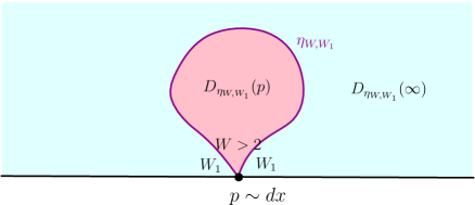
Figure 10. Illustration of welding equation (8.1.3) in Conjecture 8.2: first sample a root point $p$ according to Lebesgue measure $dx$ on $\mathbb{R}$, then sample $(\phi,\eta)$ according to the product measure $\mathrm{LF}^{(\beta_{2W_{1}+W},p)}_{\mathbb{H}}(d\phi)\times\mathrm{SLE}_{\kappa,p}^{\mathrm{bubble}}(W,W_{1})(d\eta)$. The resulting quantum surface $(\mathbb{H},\phi,\eta,p)/\sim_{\gamma}$ has the law of $C\int_{0}^{\infty}\mathcal{M}^{\mathrm{disk}}_{0,2}(W_{1};\cdot,\ell)\times\mathrm{QD}_{0,1}(\gamma,\beta_{W};\ell)d\ell$ after uniform embedding.

Conjecture 8.2.

Fix $W_{1}\geq\frac{\gamma^{2}}{2}$ and $W>2$. There exist a $\sigma$-finite infinite measure $\mathrm{SLE}^{\mathrm{bubble}}_{\kappa,p}(W,W_{1})$ on $\mathrm{Bubble}_{\mathbb{H}}(p)$ and some constant $C\in(0,\infty)$ such that

(8.1.3) $$\mathbf{m}_{\mathbb{H}}\ltimes\left(\int_{0}^{\infty}\mathcal{M}^{\mathrm{disk}}_{0,2}(W_{1};\cdot,\ell)\times\mathrm{QD}_{0,1}(\gamma,\beta_{W};\ell)d\ell\right)=C\cdot\mathrm{LF}^{(\beta_{2W_{1}+W},p)}_{\mathbb{H}}\times\mathrm{SLE}_{\kappa,p}^{\mathrm{bubble}}(W,W_{1})dp.$$

Furthermore, there exists some constant $C\in(0,\infty)$ such that

(8.1.4) $$\mathbf{m}_{\mathbb{H},0}\ltimes\left(\int_{0}^{\infty}\mathcal{M}^{\mathrm{disk}}_{0,2}(W_{1};\cdot,\ell)\times\mathrm{QD}_{0,1}(\gamma,\beta_{W};\ell)d\ell\right)=C\cdot\mathrm{LF}_{\mathbb{H}}^{(\beta_{2W_{1}+W},0)}(d\phi)\times\mathrm{SLE}_{\kappa,0}^{\mathrm{bubble}}(W,W_{1}),$$

where $\mathbf{m}_{\mathbb{H},0}$ is a Haar measure on $\mathrm{conf}(\mathbb{H},0)$, i.e., the group of conformal automorphisms of $\mathbb{H}$ fixing $0$.

In Conjecture 8.2, by the quantum triangle welding and the induction techniques developed in Section 4, we can show that 1) $\phi$ has the law of $C\cdot\mathrm{LF}_{\mathbb{H}}^{(\beta_{2W_{1}+W},0)}$, and 2) the welding interface $\eta_{W,W_{1}}$ is independent of $\phi$.

However, we have almost zero understanding on the law of $\eta_{W,W_{1}}$, i.e., $\mathrm{SLE}^{\mathrm{bubble}}_{\kappa,0}(W,W_{1})$. Recall that in Zhan’s limiting constructions of $\mathrm{SLE}_{\kappa}(\rho)$ bubbles, one takes the weak limit of chordal $\mathrm{SLE}_{\kappa}(\rho)$ under suitable rescaling. Therefore, in LQG frameworks, we take “quantum version” of the limit by 1) conditioning on the (one-side) quantum boundary length of $\mathcal{M}^{\mathrm{disk}}_{1,2}(2)$ goes to zero 2) constructing a coupling with the limiting picture so that, with high probability, the random domains match.

Nonetheless, this technique will not work in the case of Conjecture 8.2, or in a more straightforward way, $\eta_{W,W_{1}}$ is not the weak limit of chordal $\mathrm{SLE}_{\kappa}(W-2,W_{1}-2)$ under suitable rescaling. Suppose one takes $\mathcal{M}^{\mathrm{disk}}_{1,2}(W)$ and then conditioning on the (one-side) quantum boundary length goes to zero, the limiting quantum surface will always be the same; the boundary marked point is always quantum typical (cf. [MSW21, Appendix A]). In other words, we will always get $\mathrm{SLE}_{\kappa,0}^{\mathrm{bubble}}(W_{1}-2)$. Therefore, shrinking (one-side) quantum boundary length and coupling will only work for $\mathcal{M}^{\mathrm{disk}}_{1,2}(2)$.

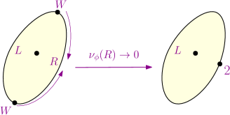
Figure 11. On the LHS, we have $\mathcal{M}^{\mathrm{disk}}_{1,2}(W)$. Conditioning on the quantum boundary length of the right arc $R$ shrinks to zero, we will get a $\mathcal{M}^{\mathrm{disk}}_{1,1}(2)$, i.e., $\mathrm{QD}_{1,1}$. Notice that in [MSW21, Appendix A], the weight $W$ is in the restricted range. However, we believe that this is only a technical barrier and will not affect the overall outcome.

Hence, one interesting question is that how to describe the law of $\eta_{W,W_{1}}$ in Conjecture 8.2? If better, what is its corresponding Lowener evolution (driving function)?

Also, going back to the Euclidean settings, in Zhan’s constructions of $\mathrm{SLE}_{\kappa}(\rho)$ bubbles, one takes the weak limit of $\mathrm{SLE}^{\mathbb{H}}_{\kappa,(\varepsilon;\varepsilon^{+})\to 0}(\rho)$ or $\mathrm{SLE}^{\mathbb{H}}_{\kappa,(0;0^{-})\to\varepsilon}(\rho)$ under suitable rescaling. Either way, that single force point of $\mathrm{SLE}_{\kappa}$ is on the outside (see Figure 3).

Hence, what if you have two force points? In other words, what if we take the weak limit of $\mathrm{SLE}^{\mathbb{H}}_{\kappa,(0;0^{-},0^{+})\to\varepsilon}(\rho_{-},\rho_{+})?$ I conjecture that it is the $\mathrm{SLE}^{\mathrm{bubble}}_{\kappa,0}(\rho_{-})$. Similarly, if we take the weak limit of $\mathrm{SLE}^{\mathbb{H}}_{\kappa,(\varepsilon;\varepsilon^{-},\varepsilon^{+})\to 0}(\rho_{-},\rho_{+})$, then it is $\mathrm{SLE}^{\mathrm{bubble}}_{\kappa,0}(\rho_{+})$.

A somewhat similar question as above is what happens to the inner force point after collapsing the $\varepsilon$ with $0$. Do they vanish? I conjecture that yes, the inner force point vanishes once collapsed.

8.2. Generalized $\mathrm{SLE}$ bubbles on $\mathbb{H}$: multiple case

Going one step further, motivated by the induction procedure described in Figure 9, we are also interested in understanding the multiple $\mathrm{SLE}$ bubbles on $\mathbb{H}$. Specifically, consider welding of three quantum disks

(8.2.1) $$\int_{0}^{\infty}\int_{0}^{\infty}\mathrm{QD}_{0,1}(\gamma,\beta_{W};\ell)\times\mathcal{M}^{\mathrm{disk}}_{0,2}(W_{1},\ell,r)\times\mathcal{M}^{\mathrm{disk}}_{0,2}(W_{2};r,\cdot)drd\ell$$

for $W\geq 2,W_{1}>0$ and $W_{2}>0$.

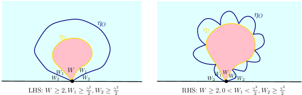
Figure 12. Illustration of quantum surface (8.2.1) when embedded in $(\mathbb{H},\phi,\eta_{I},\eta_{O})$.

Let $(\mathbb{H},\phi,0,\eta_{I},\eta_{O})$ be an particular embedding of (8.2.1) (see Figure 12), then it is not hard to show that the joint law of $(\eta_{I},\eta_{O})$ is independent of $\phi$. Moreover, the condition law $(\eta_{O}|\eta_{I})$ should equal to $\mathrm{SLE}_{\kappa,0}^{\mathrm{bubble}}(W_{1},W_{2})$ and the law of $(\eta_{I}|\eta_{O})$ should equal to $\mathrm{SLE}_{\kappa,0}^{\mathrm{bubble}}(W,W_{1})$. Recall that $\mathrm{SLE}_{\kappa,0}^{\mathrm{bubble}}(\cdot,\cdot)$ is the welding interface in Conjecture 8.2.

The interesting questions to the SLE research communities are what is the marginal law of $\eta_{\bullet},\bullet\in\{I,O\}$. Moreover, what is the Loewner evolution (driving function) of $\eta_{\bullet},\bullet\in\{I,O\}$?

8.3. Scaling limits of bubble-decorated quadrangulated disks

Recall that in the $\mathrm{SLE}$ loop case [AHS22], $\mathrm{MS}^{n}\otimes\mathrm{SAW}^{n}$ is the measure on pairs $(M,\eta)$, where $M$ is a quadrangulation, $\eta$ is a self-avoiding loop on $M$, and each $(M,\eta)$ has weight $n^{5/2}12^{-\#\mathcal{F}(M)}54^{-\#\eta}$, where $\#\mathcal{F}(M)$ denotes the number of faces of $M$ and $\#\eta$ is the number of edges of $\eta$. It is proved that the following convergence result holds.

Theorem 8.3 ([AHS22, Theorem 1.2]).

There exists constant $c_{0}>0$ and for all $c\in(0,1)$,

(8.3.1) $$\mathrm{MS}^{n}\otimes\mathrm{SAW}^{n}|_{A(c)}\xrightarrow{w}c_{0}\cdot\mathrm{QS}\otimes\mathrm{SLE}_{8/3}^{{\mathrm{loop}}}|_{A(c)},$$

where $A(c)$ is the event that the length of the loop is in $[c,c^{-1}]$.

In the disk case, we say a planar map $D$ is a quadrangulated disk if it is a planar map where all faces have four edges except for the exterior face, which has arbitrary degree and simple boundary. Let $\partial D$ denote the edges on the boundary of the exterior face, and we denote $\#\partial D$ the boundary length of $D$. Let $\mathrm{MD}^{n}$ be the measure on the quadrangulated disks such that each disk $D$ has weight $n^{5/2}12^{-\#\mathcal{F}(D)}54^{-\#\partial D}$, which has the same scaling as $\mathrm{MS}^{n}$ above. Note that here if $D$ is sampled from $\mathrm{MD}^{n}$, then $D$ is viewed as a metric measure space by considering the graph metric rescaled by $2^{-1/2}n^{-1/4}$ and giving each vertex mass $2(9n)^{-1}$.

If $D$ is a quadrangulated disk, then we say $\eta$ is a self-avoiding bubble on $D$ rooted at $e_{r}\in\partial D$ if $\eta$ is an orderer set of edges $e_{1},\ldots,e_{2k}\in\mathcal{E}(D)$ with $r\in\{1,\ldots,2k\}$ and $e_{j}$ and $e_{i}$ share an end-point if and only if $|i-j|\leq 1$ or $(i,j)\in\{(1,2k),(2k,1)\}$.

Let $\mathrm{MD}^{n}\otimes\partial\mathrm{MD}^{n}\otimes\mathrm{SAB}^{n}$ denote the measure on pairs $(D,e,\eta)$ where $\eta$ is a self-avoiding bubble on $D$ rooted at edge $e\in\partial D$ and the pair $(D,\eta)$ has weight $\#\partial D^{-1}\cdot n^{5/2}12^{-\#\mathcal{F}(D)}54^{-\#\eta}$. For $(D,e,\eta)$ sampled from $\mathrm{MD}^{n}\otimes\partial\mathrm{MD}^{n}\otimes\mathrm{SAB}^{n}$, we view $D$ as a metric measure space and view $\eta$ as a bubble on this metric measure space rooted at edge $e$ so that the time it takes to traverse each edge on the loop is $2^{-1}n^{-1/2}$.

Conjecture 8.4.

There exists some $c_{0}>0$ such that for all $c\in(0,1)$,

(8.3.2) $$\mathrm{MD}^{n}\otimes\partial\mathrm{MD}^{n}\otimes\mathrm{SAB}^{n}|_{A(c)}\xrightarrow{w}c_{0}\cdot\mathrm{LF}_{\mathbb{H}}^{(\beta_{6},p)}\times\mathrm{SLE}_{8/3,p}^{\mathrm{bubble}}\times dp|_{A(c)},$$

in Gromov-Hausdorff-Prokhorov-uniform topology, where $A(c)$ is event that the length of the bubble is in $[c,c^{-1}]$.

We can also understand the measure $\mathrm{MD}^{n}\otimes\partial\mathrm{MD}^{n}\otimes\mathrm{SAB}^{n}$ from the welding perspective. Suppose $\overline{\mathrm{MD}^{n}}$ is a measure on qudrangulated disks such that each disk $\overline{D}$ has weight $n^{5/2}12^{-\#\mathcal{F}(\overline{D})}54^{-2\#\partial\overline{D}}$ and $\underline{\mathrm{MD}^{n}}$ is a measure on qudrangulated disks with each disk $\underline{D}$ has weight $n^{5/2}12^{-\#\mathcal{F}(\underline{D})}54^{-\#\partial\underline{D}}$. Let $\overline{\mathrm{MD}_{0,2}^{n}}$ be the measure on $(\overline{D},e_{1},e_{2})$ such that we first sample $\overline{D}$ from reweighted measure $(\#\partial\overline{\mathrm{MD}^{n}})^{2}\overline{\mathrm{MD}^{n}}$ and then sample two edges $e_{1},e_{2}$ uniformly on $\partial\overline{D}$. Similarly, let $\underline{\mathrm{MD}^{n}_{0,1}}$ be the measure on $(\underline{D},e)$ such that we first sample $\underline{D}$ from reweighted measure $(\#\partial\underline{\mathrm{MD}^{n}})\cdot\underline{\mathrm{MD}^{n}}$ and then sample an edge $e$ from $\partial\underline{D}$ uniformly.

For $k\in\mathbb{N}$, let $\overline{\mathrm{MD}_{0,2}^{n}}(\cdot,k)$ denote the restriction of $\overline{\mathrm{MD}_{0,2}^{n}}$ to the event that right boundary has length $2k$ and let $\underline{\mathrm{MD}_{0,1}^{n}}(k)$ denote the restriction of $\underline{\mathrm{MD}_{0,1}^{n}}$ to the event that the total boundary has length $2k$. Let $\overline{\mathrm{MD}_{0,2}^{n}}(\cdot,k)^{\#}$ and $\underline{\mathrm{MD}_{0,1}^{n}}(k)^{\#}$ denote the corresponding probability measure respectively.

Suppose $(\overline{D},e_{1},e_{2})$ is sampled from $\overline{\mathrm{MD}_{0,2}^{n}}(\cdot,k)^{\#}$ and $(\underline{D},e)$ is sampled from $\underline{\mathrm{MD}_{0,1}^{n}}(k)^{\#}$, then we can do the “discrete conformal welding” by identifying the right boundary of $\overline{D}$ to the total boundary of $\underline{D}$ such that $e_{1},e_{2}$ and $e$ are identified. The self-avoiding bubble on the discrete disk represents the welding interface of $\overline{D}$ and $\underline{D}$. We parametrize the bubble so that each edge on the bubble has length $2^{-1}n^{-1/2}$ just like the sphere case. Suppose $(\overline{D},e_{1},e_{2})$ is sampled from $\overline{\mathrm{MD}_{0,2}^{n}}(\cdot,k)^{\#}$ and $(\underline{D},e)$ is sampled from $\underline{\mathrm{MD}_{0,1}^{n}}(k)^{\#}$, then we denote the measure on the disks decorated with a self-avoiding bubble sampled in this way by $\mathrm{Weld}_{d}^{\mathrm{bubble}}(\overline{\mathrm{MD}_{0,2}^{n}}(\cdot,k)^{\#},\underline{\mathrm{MD}_{0,1}^{n}}(k)^{\#})$. Similarly, let $\mathrm{Weld}_{c}^{\mathrm{bubble}}(\mathrm{QD}_{0,2}(\cdot,\ell)^{\#},\mathrm{QD}_{0,1}(\ell)^{\#})$ denote the measure on bubble-decorated quantum disk obtained by identifying the right boundary of the disk sampled from $\mathrm{QD}_{0,2}(\cdot,\ell)^{\#}$ and the total boundary of the disk sampled from $\mathrm{QD}_{0,1}(\ell)^{\#}$.

Conjecture 8.5.

For any $\ell>0$, we have

(8.3.3) $$\mathrm{Weld}_{d}^{\mathrm{bubble}}(\overline{\mathrm{MD}_{0,2}^{n}}(\cdot,[\ell n^{1/2}])^{\#},\underline{\mathrm{MD}_{0,1}^{n}}([\ell n^{1/2}])^{\#})\xrightarrow{w}\mathrm{Weld}_{c}^{\mathrm{bubble}}(\mathrm{QD}_{0,2}(\cdot,\ell)^{\#},\mathrm{QD}_{0,1}(\ell)^{\#})$$

in Gromov-Hausdorff-Prokhorov-uniform topology.

References

- [AHS20] Morris Ang, Nina Holden, and Xin Sun. Conformal welding of quantum disks. arXiv:2009.08389v1, 2020.
- [AHS21] Morris Ang, Nina Holden, and Xin Sun. Integrability of SLE via conformal welding of random surfaces. arXiv:2104.09477v1, 2021.
- [AHS22] Morris Ang, Nina Holden, and Xin Sun. The loop via conformal welding of quantum disks. arXiv:2205.05074v1, 2022.
- [ARS22] Morris Ang, Guillaume Remy, and Xin Sun. FZZ formula of boundary liouville CFT via conformal welding. arXiv:2104.09478v3, 2022.
- [ARSZ23] Morris Ang, Guillaume Remy, Xin Sun, and Tunan Zhu. Derivation of all structure constants for boundary Liouville CFT. ArXiv eprint, 2023.
- [AS21] Morris Ang and Xin Sun. Integrability of the conformal loop ensemble. arXiv:2107.01788, 2021.
- [ASY22] Morris Ang, Xin Sun, and Pu Yu. Quantum triangles and imaginary geometry flow lines. arXiv:2211.04580v1, 2022.
- [BPZ84] A.A. Belavin, A.M. Polyakov, and A.B. Zamolodchikov. Infinite conformal symmetry in two-dimensional quantum field theory. Nuclear Physics B, 241(2):333–380, 1984.
- [DKRV16] François David, Antti Kupiainen, Rémi Rhodes, and Vincent Vargas. Liouville quantum gravity on the riemann sphere. Communications in Mathematical Physics, 342(3):869–907, 2016.
- [DMS20] Bertrand Duplantier, Jason Miller, and Scott Sheffield. Liouville quantum gravity as a mating of trees. arXiv: 1409.7055, 2020.
- [DRV15] François David, Rémi Rhodes, and Vincent Vargas. Liouville quantum gravity on the complex tori. Journal of Mathematical Physics, 57, 04 2015.
- [FZZ00] V. Fateev, Alexander B. Zamolodchikov, and Alexei B. Zamolodchikov. Boundary Liouville field theory. 1. Boundary state and boundary two point function. Eprint: hep-th/0001012, 1 2000.
- [GRV19] Colin Guillarmou, Rémi Rhodes, and Vincent Vargas. Polyakov’s formulation of 2d bosonic string theory. Publications mathématiques de l’IHÉS, 130(1):111–185, 2019.
- [Hos01] Kazuo Hosomichi. Bulk-boundary propagator in liouville theory on a disc. Journal of High Energy Physics, 2001(11):044, Dec. 2001.
- [HRV18] Yichao Huang, Rémi Rhodes, and Vincent Vargas. Liouville quantum gravity on the unit disk. Annales de l’Institut Henri Poincaré, Probabilités et Statistiques, 54(3):1694–1730, 2018.
- [KRV17] Antti Kupiainen, Rémi Rhodes, and Vincent Vargas. Integrability of Liouville theory: proof of the DOZZ Formula. Annals of Mathematics, 191, 07 2017.
- [MSW21] Jason Miller, Scott Sheffield, and Wendelin Werner. Simple Conformal Loop Ensembles on Liouville Quantum Gravity. arXiv: 2002.05698, 2021.
- [Pol81] A.M. Polyakov. Quantum geometry of bosonic strings. Physics Letters B, 103(3):207–210, 1981.
- [Rem17] Guillaume Remy. Liouville quantum gravity on the annulus. Journal of Mathematical Physics, 2017.
- [Rem20] Guillaume Remy. The fyodorov-bouchaud formula and liouville conformal field theory. Duke Math. J., 169(1):177–211, 2020.
- [RZ20] Guillaume Remy and Tunan Zhu. The distribution of gaussian multiplicative chaos on the unit interval. The Annals of Probability, 48(2):872–915, 2020.
- [RZ22] Guillaume Remy and Tunan Zhu. Intergrability of boundary liouville conformal field theory. Communications in Mathematical Physics, 395(1):179–168, 2022.
- [She10] Scott Sheffield. Conformal weldings of random surfaces: Sle and the quantum gravity zipper. The Annals of Probability, 44, 12 2010.
- [Zha19] Dapeng Zhan. Decomposition of schramm-lowener evolution along its curve. Stochastic Processes and their Applications, 129:129–152, 2019.
- [Zha22] Dapeng Zhan. bubble measures. arXiv:2206.04481v1, 2022.