A Counterexample to the Lévy Flight Foraging Hypothesis in the Narrow Capture Framework

Abstract.

The Lévy flight foraging hypothesis asserts that biological organisms have evolved to employ (truncated) Lévy flight searches due to such strategies being more efficient than those based on Brownian motion. However, we provide here a concrete two-dimensional counterexample in which Brownian search is more efficient. In fact, we show that the efficiency of Lévy searches worsens the farther the Lévy flight tail index deviates from the Brownian limit. Our counterexample is based on the framework of the classic narrow capture problem in which a random search is performed for a small target within a confined search domain. Our results are obtained via three avenues: Monte Carlo simulations of the discrete search processes, finite difference solutions and a matched asymptotic analysis of the elliptic (pseudo)-differential equations of the corresponding continuum limits.

Keywords: Hopf bifurcations, small eigenvalues, localized solutions, domain geometry

It is a widely held belief that random search algorithms using Lévy flights can find a target faster than using Brownian motion [35, 45, 46]. This so called “Lévy flight foraging hypothesis” forms the basis of many biological models (e.g., [44, 31]) as well as numerical search algorithms [45, 20, 50, 49, 16]. It has also led the seeking of optimal Lévy tail indices (e.g., [45, 22]) for maximizing the amount of sparsely spaced targets being captured relative to the distance traversed [45], resulting in the 2020-21 dialogue that took place on Phys. Rev. Lett. [22, 6, 23].

In contrast to these existing works, we present an alternative means of quantifying efficiency via measuring the expected search time of a small target in a finite domain and provide an example in two-dimensions for which the Brownian search strategy is more efficient than strategies based a Lévy flight of any tail index $\alpha$. In fact, we demonstrate that in our setting, a certain power-law dependence of the search time on $\alpha$ that worsens the farther $\alpha$ deviates from its Brownian limit. The framework we employ for this comparison is consistent with that of first passage time problems (e.g., [30, 1, 2, 37]) in a geometry motivated by the narrow capture problem used to model biological and ecological processes (e.g., [34, 18, 17, 36, 3, 29, 21, 14]).

We develop three different approaches to arrive at our result. First, we devise and implement a Monte Carlo simulation to calculate the expected search time of searches based on Lévy flight. Second, we implement a numerical method for solving (pseudo)-differential equations which yields detailed information about the expected search time as a function of initial position. We use this numerical solution to gain insight into the potential mechanism behind why Brownian searches appear to take less time than Lévy flights. Third, in the Appendix B, we develop a matched asymptotic analysis to derive leading order analytic predictions for the expected search times. We remark that the comprehensive set of results from these three different approaches provide more quantitative and qualitative insight than the analytic asymptotic estimate for the search time discussed recently in [7].

A schematic of the narrow escape framework for the geometry we consider is shown in Fig. 1. The search domain is the unit torus $\mathbb{T}^{2}$ of unit side length with periodic boundary conditions and bottom left vertex at the origin. Two instances are shown of paths traced out by a Brownian (green) and Lévy (blue) search for a target of disc of radius $\epsilon$ centered at $\mathbf{x}_{0}=(1/2,1/2)$ (red). The pink dots mark the locations $\mathbf{x}$ from where the respective searches begin. The search ends when the search first lands either on the boundary or inside the target disk.

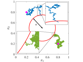
Figure 1. Illustration of Lévy flight (blue) and Brownian walk (green) searches for a target of disc of radius $\epsilon=0.25$ (red circle indicates its boundary) centered at the point $(0.5,0.5)$ on the flat torus $\mathbb{T}^{2}$. The pink markers indicate the starting locations of each search. Each search continues until it first reaches the target. Closeups of both paths are shown in insets. The Lévy search path (tail index $\alpha=0.5$) exhibits series of small jumps separated by occasional long jumps while the Brownian path lacks the latter. Note that $\epsilon$ is set relatively large for illustrative purposes; we consider a smaller range of $\epsilon$ in this Letter.

The qualitative differences in the two paths are due to the probability distributions of their respective jump lengths. For the Brownian search, jump lengths are normally distributed with zero mean and variance of $\Delta t$ sufficiently small, leading to the linear-in-time mean squared displacement $\langle|\Delta\mathbf{x}|^{2}\rangle\propto\Delta t$. In the Lévy search with tail index $0<\alpha<1$, jump lengths $|\mathbf{y}|$ are given by $|\mathbf{y}|=(\Delta t)^{1/(2\alpha)}|\mathbf{k}|$, where $\mathbf{k}$ is distributed according to a power-law distribution with tail $\sim|\mathbf{k}|^{-(2+2\alpha)}$ (see, e.g., [26, 43, 15, 27, 1] and references therein). This leads to an unbounded mean squared displacement, and the super-linear scaling $\langle|\Delta\mathbf{x}|^{2\delta}\rangle^{1/\delta}\propto(\Delta t)^{1/\alpha}$ for $\delta<\alpha$.

In the next section, we present our main findings and give possible reasons for the inferiority of Lévy search strategies within the narrow escape framework.

1. Main results and interpretation

For a random search on $\mathbb{T}^{2}$, let us denote $u_{\epsilon}(\mathbf{x})$ ($v_{\epsilon}(\mathbf{x})$) the average search time (i.e., mean first passage time, or MFPT) of a Lévy (Brownian) search starting from location $\mathbf{x}$, and $B_{\epsilon}(\mathbf{x}_{0})$ the circular target of radius $\epsilon$ centered at $\mathbf{x}_{0}$. Then the global mean first passage time (GMFPT) [37] is the expected search time averaged uniformly over all starting points $\mathbf{x}\in\mathbb{T}^{2}\setminus B_{\epsilon}(\mathbf{x}_{0})$. That is, the GMFTP, $\bar{u}_{\epsilon}$, of the Lévy search is given by $\bar{u}_{\epsilon}=\int_{\mathbb{T}^{2}\setminus B_{\epsilon}(\mathbf{x}_{0})}\!u_{\epsilon}(\mathbf{x})\,d\mathbf{x}$, and similarly for the GMFPT, $\bar{v}_{\epsilon}$, of the Brownian search.

We show in Fig. 2 our primary result demonstrating that Brownian search is on average faster than Lévy search. Moreover, the Lévy flight search time increases the more its tail index $\alpha$ deviates from its Brownian limit of $1$. In the figure, we plot the Lévy search GMFPT $\bar{u}_{\epsilon}$ for three different tail indices and for a range of target sizes $\epsilon$ on a log-log scale. The blue x’s are obtained from Monte Carlo simulations (see Fig. 1), which we discuss below. The black o’s are obtained from finite difference solutions of the elliptic pseudo-differential equation for $u_{\epsilon}(\mathbf{x})$ given by (3.1a) corresponding to the continuum limit of the Monte Carlo process. Both confirm the leading order analytic result (shown in red) derived via a matched asymptotic analysis in (B.22) of Appendix B, stating that in the limit $\epsilon\to 0^{+}$ with $0<\alpha<1$,

$$\bar{u}_{\epsilon}\sim A_{\alpha}\epsilon^{2\alpha-2}\,;\quad A_{\alpha}:=\frac{\Gamma(1-\alpha)(1-\alpha)}{4^{\alpha}\Gamma(\alpha)\sin((1-\alpha)\pi)}\,.$$ (1.1)

The error of this approximation grows as $\alpha$ nears its Brownian limit of $1$, accounting for the worsening discrepancies between the blue x/black o and the (red) analytic prediction as $\alpha$ gets closer to $1$. We also plot $\bar{v}_{\epsilon}$, the GMFPT of the Brownian search, obtained from numerically solving (3.2a) (black o’s). The red dashed curve plots the functional form $-(2\pi)^{-1}\log(\epsilon)+c$ for some constant $c$, confirming the well-known the leading order $\mathcal{O}(|\log\epsilon|)$ scaling of Brownian search times (see, e.g., [34, 18, 17, 36, 3, 29]).

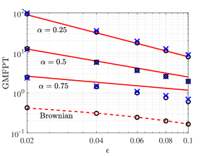
Figure 2. (a) For Lévy flight tail index $\alpha=0.25$, $\alpha=0.5$, $\alpha=0.75$, and Brownian motion, with target of radius $\epsilon$ centered at $(1/2,1/2)$, we plot the GMFPT versus $\epsilon$. The results indicate that Brownian search is faster on average than the three Lévy searches considered, and that average search times increase further the tail index $\alpha$ is from its Brownian limit of $1$. The quantities plotted in blue x’s and black o’s are obtained from Monte Carlo simulations and numerical solutions of the corresponding elliptic (pseudo)-differential equations, respectively. The solid red lines indicate the leading order power-law scaling of (1.1) given by (B.22) of Appendix B, while the dashed red curve plots the functional form $-(2\pi)^{-1}\log(\epsilon)+c$ for some constant $c$.

We give a possible explanation for the longer average duration of Lévy searches. In Figs. 3, we plot the finite difference solution for $u_{\epsilon}(\mathbf{x})$ when $\alpha=1/2$ and $\epsilon=0.03$, and compare a cross section of this solution to that of $v_{\varepsilon}(\mathbf{x})$. In Fig. 3(b), we first observe that both solutions are identically $0$ for $\mathbf{x}\in B_{\epsilon}(\mathbf{x}_{0})$ (i.e., searches beginning in and on the target cost zero time). Near the target boundary, we observe a much sharper rise in $u_{\epsilon}$ than for $v_{\epsilon}$, while far from the target, $u_{\epsilon}$ is flatter than $v_{\epsilon}$. This behavior of $u_{\epsilon}$ suggests that proximity to the target of starting location has little impact on the Lévy search time. This owes to there being a greater likelihood of taking a long jump in the “wrong” direction, especially when the target is small.

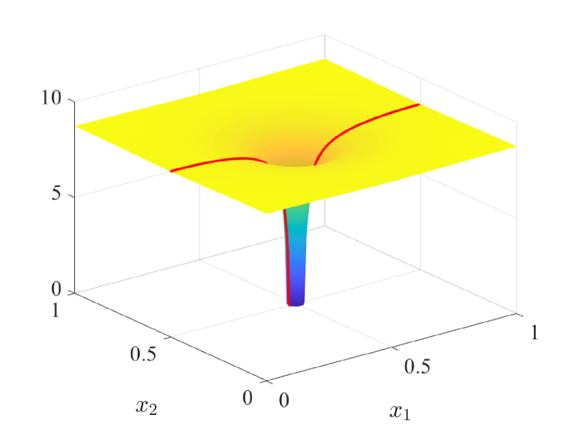
(a) $u_{\epsilon}(p)$

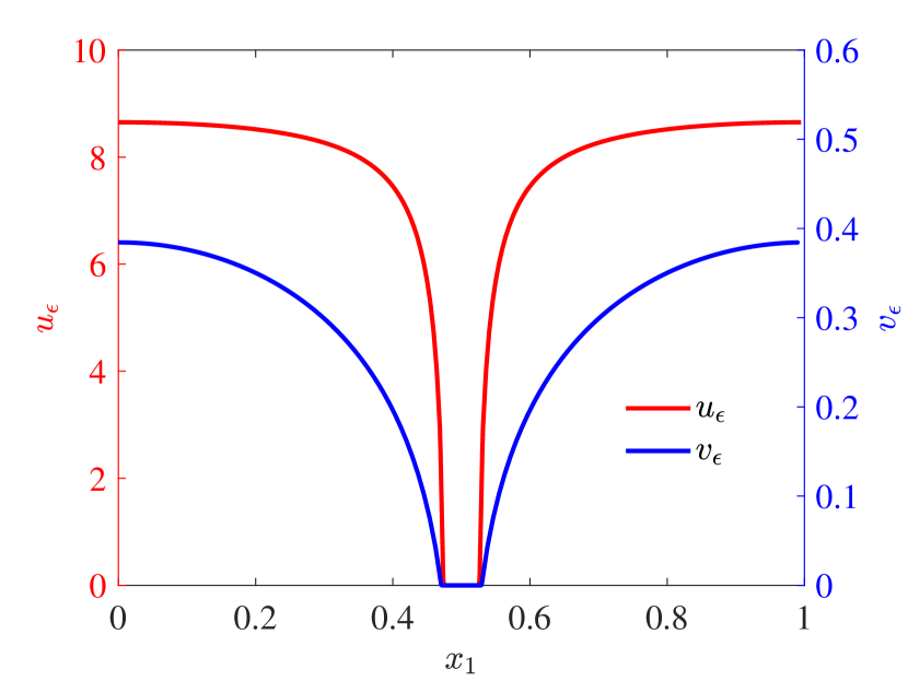
(b) horizontal cross-section of $u_{\epsilon}$, $v_{\epsilon}$

Figure 3. For $\alpha=1/2$ with target of radius $\epsilon=0.03$ centered at $(1/2,1/2)$, we show in (a) the numerical solution for $u_{\epsilon}$ of (3.1a). The red line indicates the contour plotted in red and (b), where, in blue, we also plot the corresponding contour of the numerical solution $v_{\epsilon}$ of (3.2a). Note that $u_{\epsilon}$ ($v_{\epsilon}$) is plotted on the left (right) vertical axis. The spatial average of $u_{\epsilon}$ is approximately $8.57$ while that of $v_{\epsilon}$ is approximately $0.357$, indicating that an average search conducted via the Lévy process with $\alpha=1/2$ for a small target will be significantly longer in comparison.

Thus, a Lévy search that has reached the vicinity of the target may take a long jump away from it, effectively forcing it to restart its search from a farther location. Repeated approaches to the target followed by long jumps away from it can lead to anomalously long search times, which we show in Fig. 4(a). Obtained from Monte Carlo simulations of search processes beginning at $(0,0)$, the probability density distributions of Lévy search times differ greatly from that of Brownian search times. In particular, the comparatively slow decay of the tail for longer search times is apparent, especially for $\alpha=1/4$. The greater variance of Lévy search times is confirmed in Fig. 4(b), where we show finite difference computations of the search time variance averaged over all starting locations. We note the near-linear behavior of Lévy flight variances, suggesting that they, along with the GMFPT $\bar{u}_{\epsilon}$, follow a power-law scaling.

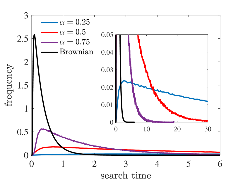
(a) distribution of search times

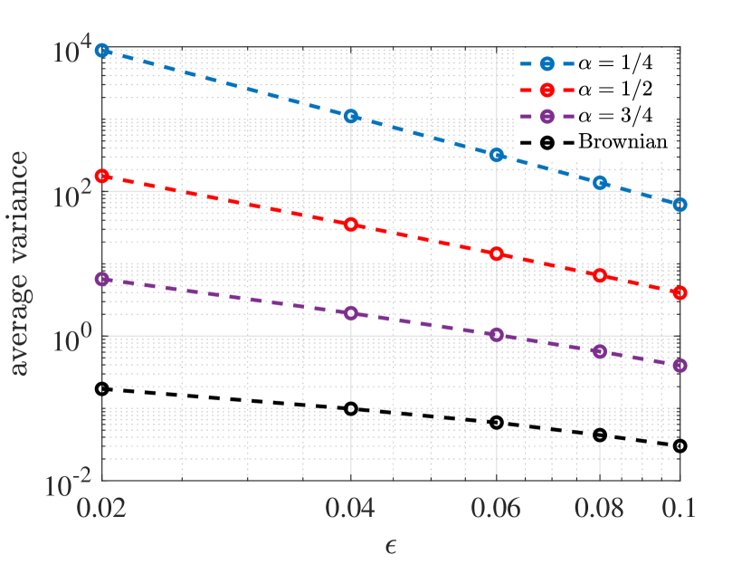
(b) average variance

Figure 4. (a) Starting from the point $(0,0)$, the figure shows the full probability density function of search times for a target of radius $\epsilon=0.04$ centered at $p_{0}=(1/2,1/2)$. Results for the Brownian search are obtained from numerically solving the time-dependent diffusion PDE while those for the Lévy searches are obtained from Monte Carlo simulations. Observe the increasingly heavy tail of the distributions as $\alpha$ decreases. This indicates the increasing likelihood of long search times, contributing to the longer average search times of Lévy flights relative to Brownian walks. (b) Finite difference computation of (3.1c) and (3.2b) of search time variance averaged over all starting locations.

In the following sections, we provide an overview of our methodology, beginning with a brief outline of our Monte Carlo algorithm . We then give the elliptic pseudo-differential equations which characterize the continuum limit of the Lévy search process. Mathematical details are presented the Appendix. We close by discussing some open problems.

2. Monte Carlo Simulation of Lévy Flight Search on $\mathbb{T}^{2}$

We describe here the Monte Carlo algorithm that we used to generate the simulated Lévy flight search times of the previous section. The algorithm is motivated by the description of Lévy flights on $\mathbb{R}^{n}$ given by Valdinoci [43]. We describe the process on $\mathbb{R}^{2}$ from which we can derive the process on $\mathbb{T}^{2}$ simply by identifying $(n+r,m+s)\equiv(r,s)$ for $n,m\in\mathbb{Z}$ and $r,s\in(0,1)$.

For the $(j+1)-th$ step starting from $\mathbf{x}_{j}\in\mathbb{T}^{2}$ with $j=0,1,2,\ldots$, the $j$-th displacement of the Lévy flight with tail index $0<\alpha<1$ is given by $h\mathbf{k}$, where $h$ is a sufficiently small parameter and $\mathbf{k}\in\mathbb{Z}^{2}$ is a random variable drawn from a power-law distribution with tail $\sim~{}|\mathbf{k}|^{-2-2\alpha}$. Since $\langle|\mathbf{k}|^{2\delta}\rangle$ is bounded for $0<\delta<\alpha<1$, we have the scaling of the expected displacement $\langle|\Delta\mathbf{x}|^{2\delta}\rangle\propto h^{\delta}$, or $\langle|\Delta\mathbf{x}|^{2\delta}\rangle^{2/\delta}\propto h^{2}$. We then let $\Delta t=D_{\alpha}h^{2\alpha}$ so that $\langle|\Delta\mathbf{x}|^{2\delta}\rangle^{2/\delta}\propto(\Delta t)^{1/\alpha}$ as required. Here, $D_{\alpha}$ is a constant chosen so that the process is consistent with Brownian motion in the limit $\alpha\to 1^{-}$ (see (A.18) of Appendix A). As mentioned above, from this jump process on $\mathbb{R}^{2}$ one can deduce the process on $\mathbb{T}^{n}$ simply by modding out $\mathbb{Z}^{2}$.

We simulate this process on $\mathbb{T}^{2}$ until the position $\mathbf{x}_{N+1}$ of the search first encounters $\overline{B_{\epsilon}(\mathbf{x}_{0})}$. The duration of the search is then given by $N\Delta t$, where $\Delta t=D_{\alpha}h^{2\alpha}$. The search beginning from $\mathbf{x}_{1}$ is repeated for $500,000$ iterations, the average search time of which is taken to be the simulated MFPT starting from $\mathbf{x}_{1}$. The GMFPT is obtained by varying the starting location $\mathbf{x}_{1}$ over $\mathbb{T}^{2}$, repeating the process, then averaging over all starting locations. We note that results did not change significantly when $1\times 10^{6}$ iterations were run from each starting location instead of $5\times 10^{5}$. More details are given in Appendix D, while the rejection sampling algorithm used to draw random variables in $\mathbb{Z}^{2}$ from a power-law distribution is given in Appendix C.

3. The Elliptic (Pseudo)-Differential Equations

In this section, we briefly discuss the elliptic pseudo-differential equation satisfied by $u_{\epsilon}(\mathbf{x})$, the MFPT of the Lévy search starting from point $\mathbf{x}\in\mathbb{T}^{2}$ in the continuous limit. Adopting the electrostatics approach of [30] for Brownian searches, we show in Appendix A that $u_{\epsilon}(\mathbf{x})$ satisfies the exterior problem

$$\mathcal{A}_{\alpha}u_{\epsilon}=-1\ {\rm on}\ \mathbb{T}^{2}\setminus\overline{B_{\epsilon}(\mathbf{x}_{0})},\ \ u_{\epsilon}=0\ {\rm on}\ \overline{B_{\epsilon}(\mathbf{x}_{0})}\,,$$ (3.1a)

where $$\mathcal{A}_{\alpha} 0<\alpha<1 \alpha \mathbb{T}^{2}$$ for is the fractional Laplacian of order on given by

$$\mathcal{A}_{\alpha}f(\mathbf{x}):=\frac{4^{\alpha}\Gamma(1+\alpha)}{\pi|\Gamma(-\alpha)|}\times\int\limits_{[0,1]\times[0,1]}\!\sum_{\mathbf{m}\in\mathbb{Z}^{2}}\frac{1}{|\mathbf{x}-(\mathbf{y}+\mathbf{m})|^{2+2\alpha}}[f(\mathbf{y})-f(\mathbf{x})]\,d\mathbf{y}\,,$$ (3.1b)

where $$\mathbf{y}+\mathbf{m} \mathbf{y}\in\mathbb{T}^{2} \mathbb{R}^{2} \mathcal{A}_{\alpha} \mathbb{T}^{2} \alpha\to 1^{-} \mathbb{R}^{2} \mathcal{A}_{\alpha} \alpha \mathbf{y} \mathbf{x} \mathbb{T}^{2} \sigma_{\epsilon}(\mathbf{x})$$ are all points corresponding to in the tiling of with unit squares. We remark that the eigenvalues of converge to that of the usual (local) Laplacian on as . Furthermore, for a Lévy flight on , the operator would simply become the standard fractional Laplacian of order given in (3.1b) of Appendix A. The lattice sum kernel of (3.1a) sums the probabilities of all the possible paths from to on . By analogy with [30, 21], we have that the variance of the MFPT, , satisfies

$$\mathcal{A}_{\alpha}\sigma_{\epsilon}=-2u_{\epsilon}(\mathbf{x})\ {\rm on}\ \mathbb{T}^{2}\setminus\overline{B_{\epsilon}(\mathbf{x}_{0})},\ \ \sigma_{\epsilon}=0\ {\rm on}\ \overline{B_{\epsilon}(\mathbf{x}_{0})}\,.$$ (3.1c)

The boundary value problems for the Brownian search time ($v_{\epsilon}(\mathbf{x})$) and variance ($\tau(\mathbf{x})$) are well-known ([30]):

$$\Delta v_{\epsilon}=-1\ {\rm on}\ \mathbb{T}^{2}\setminus\overline{B_{\epsilon}(\mathbf{x}_{0})},\ \ v_{\epsilon}=0\ {\rm on}\ \partial B_{\epsilon}(\mathbf{x}_{0})\,,$$ (3.2a)

$$\Delta\tau_{\epsilon}=-2v_{\epsilon}\ {\rm on}\ \mathbb{T}^{2}\setminus\overline{B_{\epsilon}(\mathbf{x}_{0})},\ \ \tau_{\epsilon}=0\ {\rm on}\ \partial B_{\epsilon}(\mathbf{x}_{0})\,.$$ (3.2b)

Finite difference solutions of (3.1a)-(3.2b) are straightforward, although discretizing the operator $\mathcal{A}_{\alpha}$ is computationally expensive. As such, asymptotic methods for equations of the forms (3.1a) and (3.1c), such as that provided in Appendix B, may be helpful in reducing computation requirements.

4. Discussion

Through Monte Carlo simulations, direct numerical solutions and asymptotic analysis of the limiting nonlocal exterior problem (3.1), we have shown that the average search time of a Lévy flight with tail index $0<\alpha<1$ on the flat torus $\mathbb{T}^{2}$ with a small circular target of radius $0<\epsilon\ll 1$ scales as $\mathcal{O}(\epsilon^{2\alpha-2})$. By comparing to average search times of the Brownian walk on the same domain, which obey the well-known $\mathcal{O}(|\log\epsilon|)$ scaling, we have provided a concrete counterexample to the Lévy flight foraging hypothesis. We emphasize that our comparison is limited only to the narrow escape framework, and is not a general statement on the superiority of Brownian over Lévy search strategies. One possible avenue may be to assess whether a search strategy based on a combination of Brownian motion and Lévy flight (e.g., [28]) can be optimized to be faster than pure Brownian search in the narrow escape framework.

The discrete process that we model with Monte Carlo simulations, the continuum limit of which is described by (3.1), allows the search to cross “over” the target without the target being accounted as found. It would be interesting to determine whether a Lévy process that terminates when such jumps occur is appreciably more efficient.

Lastly, while we presented results only for small target sizes $\epsilon$, we note that Lévy search times exceeded Brownian search times for all $\varepsilon<0.5$. Within this first-passage time framework, it may be insightful to seek possible scenarios in which the Lévy search strategy is superior.

We now discuss some avenues for future work, several of which are projects currently in progress. While a single target $\mathbb{T}^{2}$ is a very simple domain on which to perform this comparison, it would be interesting to consider more complex domains. For example, a finite domain with reflecting boundaries containing perhaps small reflecting obstacles may present challenges from both a modeling and analytic perspective. From a particle simulations perspective, reflective domains and obstacles would require computing trajectories of flights that undergo reflections. From the pseudo-differential equation perspective, one must formulate an analog to the $\mathcal{A}_{\alpha}$ operator of (3.1b); this new operator must account for all possible paths between all pairs of points, including those that reflect off boundaries and obstacles.

A domain featuring non-constant curvature would also present computational challenges - geodesics would need to be computed for both the Monte Carlo algorithm as well as the finite difference method for discretizing the corresponding infinitesimal generator (see [7]). This would add to the already significant computational cost. The sphere, on the other hand, has simple geodesics and may be a good candidate for a follow-up study, especially considering the interesting predictions made in [7] regarding the possible optimality of starting the search from the point antipodal to the center of the target (see Theorem 1.1 part (iii)).

Another domain feature that we have not considered is the inclusion of more than one target, one or more of which may be of non-circular shape. The multiple-target problem has been considered at length for Brownian motion on flat 2- and 3-dimensional geometries using hybrid asymptotic-numerical methods see (e.g., [14, 25, 29, 11, 13, 5, 4, 18] and the references therein). Several numerical optimization studies have been done to find optimal target arrangements that minimize the spatial average of the stopping time (e.g., [12, 9, 32, 10]). The inclusion of more than one target also gives rise to the question of splitting probabilities (see e.g., [21, 33, 8]) and shielding effects [21], and how they compare to their Brownian counterparts.

One useful aspect of such a hybrid methods is their ability to capture the higher order correction terms of the GMFPT, which encode effects of target locations/configurations. This can be accomplished by performing a higher order matching in the asymptotic solution for $u_{\varepsilon}(\mathbf{x})$ in Section B, and computing the regular part of the Green’s function $G_{\alpha}$ in (B.9). The greater ease of solving this $\epsilon$-independent problem without singular features has made possible the computational optimization studies referenced above. An analogous hybrid analytic-numerical theory for the fractional Laplacian on $\mathbb{T}^{2}$ or the more general operator on Riemannian manifolds would open various avenues of research. A similar method was recently developed for the Laplacian on Riemannian 2-manifolds using techniques in microlocal analysis [38, 41], which allowed for predictions of localized spot dynamics in reaction-diffusion systems on manifolds.

Numerical results suggest that the variance of the stopping time may have a larger scaling with $\mathcal{O}(1/\epsilon)$ than the mean. The large variance suggests that the mean of the stopping time may not be particularly informative of the probability distribution of stopping times. Asymptotic computation of the variance of the MFPT for the narrow escape problem has been done in, e.g., [21, 24] for Brownian motion. To capture all moments of the probability distribution, however, would require analysis of the diffusion equation. In [24, 3], a Laplace transform in the time variable was employed to transform the problem to an elliptic boundary value problem, on which the hybrid asymptotic-numerical tools of [47] could be applied before transforming back. A analogous approach may be possible to characterize the full distribution of stopping times of a Lévy flight on Riemannian manifolds.

Finally, for Brownian motion, the problem of finding target configurations that optimize GMFPT is closely related to the problem of finding stable equilibrium configurations of localized spots in the Schnakenberg reaction-diffusion system (cf. [39] and [10]). Furthermore, the question of whether a mobile target leads to lower GMFPT has been found to be closely related to a certain instability of the aforementioned localized spot equilibria [42, 40, 48]. It would be interesting to explore whether these relationships still hold when Brownian motion is replaced by Lévy flights.

Appendix A Derivation of elliptic (pseudo)-differential equations for average Brownian and Lévy search times

We provide here a derivation of the pseudo-differential equation for the average search time via Lévy flight of a circular target of radius $\epsilon$ starting from some point $\mathbf{x}=(x_{1},x_{2})$. The derivation is based on a continuum limit of a discrete process, and is given in [30] for a Brownian search, which we reproduce first for the purpose of completeness.

Consider a Brownian particle on an $N\times N$ grid with spacing $h=1/(N-1)$. At regular intervals of $\Delta t$, the particle hops from its current location $(x_{1},x_{2})$ to one of its four neighboring points, $(x_{1}+h,x_{2})$, $(x_{1}-h,x_{2})$, $(x_{1},x_{2}+h)$, and $(x_{1},x_{2}-h)$ with equal probability. Let $v_{\epsilon}(\mathbf{x})$ be the expected search time starting from $(x_{1},x_{2})$. Then $u_{\epsilon}(\mathbf{x})$ must be the average of the expected search time starting from one of its four neighboring points, plus the $\Delta t$ traversal time. That is,

$$v_{\epsilon}(x_{1},x_{2})=\frac{1}{4}\left[v_{\epsilon}(x_{1}+h,x_{2})+v_{\epsilon}(x_{1}-h,x_{2})+v_{\epsilon}(x_{1},x_{2}+h)+v_{\epsilon}(x_{1},x_{2}-h)\right]+\Delta t\,.$$ (A.1)

Dividing (A.1) by $\Delta t$, we have

$$\frac{h^{2}}{4\Delta t}\frac{v_{\epsilon}(x_{1}+h,x_{2})+v_{\epsilon}(x_{1}-h,x_{2})+v_{\epsilon}(x_{1},x_{2}+h)+v_{\epsilon}(x_{1},x_{2}-h)-4v_{\epsilon}(x_{1},x_{2})}{h^{2}}+1=0\,.$$ (A.2)

Taking the limit $h\to 0$ and $\Delta t\to 0$ in (A.2) while maintaining $h^{2}/(4\Delta t)=1$, we obtain

$$\Delta v_{\epsilon}+1=0\,,\quad\mathbf{x}\in\mathbb{T}^{2}\,;\qquad v_{\epsilon}=0\,,\quad\mathbf{x}\in\partial B_{\epsilon}(\mathbf{x}_{0})\,,$$ (A.3)

where the boundary condition of (A.3) is the statement that the search time starting from the boundary of the target is zero. For the unit torus $\mathbb{T}^{2}$, $v_{\varepsilon}(\mathbf{x})$ would satisfy periodic conditions on the boundary.

Following the idea of [43], we now generalize this derivation to Lévy flights characterized by a jump length distribution whose tail decays according to the power law $\sim|\mathbf{k}|^{-2-2\alpha}$ for $0<\alpha<1$. For the flat torus $\mathbb{T}^{2}$ with $\mathbf{x}\in[0,1)\times[0,1)$, we have the same $N\times N$ grid with spacing $h=1/(N-1)$. Instead of (A.1) which allows only for nearest-neighbor jumps, we have

$$u_{\epsilon}(h{\mathbf{i}})=\sum_{j_{1}=0}^{N-1}\sum_{j_{2}=0}^{N-1}w(h{\mathbf{i}},h{\mathbf{j}})u_{\epsilon}(h{\mathbf{j}})+\Delta t\,.$$ (A.4)

In (A.4), ${\mathbf{i}}=(i_{1},i_{2})\in[0,N-1]\times[0,N-1]$, ${\mathbf{j}}=(j_{1},j_{2})$, and $w(h{\mathbf{i}},h{\mathbf{j}})$ is a sum of the probabilities of all possible paths from $h{\mathbf{i}}$ to $h{\mathbf{j}}$ on $\mathbb{T}^{2}$, taking into account that there are an infinite number of ways to travel from one point to another via a straight line owing to the periodic nature of $\mathbb{T}^{2}$. From [43], a jump of $h\mathbf{k}$ has the probability given by $\mathcal{K}_{\alpha}(\mathbf{k})$, where the discrete probability mass function $\mathcal{K}_{\alpha}(\mathbf{k})$ on $\mathbb{Z}^{2}$ is given by

$$\mathcal{K}_{\alpha}(\mathbf{k})=\begin{cases}0&\mathbf{k}=\mathbf{0}\\ C_{\alpha}|\mathbf{k}|^{-2-2\alpha}&\mathbf{k}\neq\mathbf{0}\end{cases}\,,$$ (A.5a)

where $$C_{\alpha}$$ is the normalizing constant given by

$$C_{\alpha}=\frac{1}{\sum\limits_{\mathbf{k}\in\mathbb{Z}^{2}\,,\,\mathbf{k}\neq\mathbf{0}}|\mathbf{k}|^{-2-2\alpha}}\,,$$ (A.5b)

so that

$$\sum\limits_{\mathbf{k}\in\mathbb{Z}^{2}}\mathcal{K}_{\alpha}(\mathbf{k})=1\,.$$ (A.5c)

The probability of reaching $h{\mathbf{i}}$ from $h{\mathbf{j}}$ on $\mathbb{T}^{2}$ must then be given by the lattice sum

$$w(h{\mathbf{i}},h{\mathbf{j}})=\sum_{\mathbf{m}\in\mathbb{Z}^{2}}C_{\alpha}|{\mathbf{i}}-({\mathbf{j}}+\mathbf{m}(N-1))|^{-2-2\alpha}\,,$$ (A.6)

where $\mathbf{m}=(m_{1},m_{2})\in\mathbb{Z}^{2}$, and we have tiled $\mathbb{R}^{2}$ with the unit square, and ${\mathbf{j}}+\mathbf{m}(N-1)$ is the point corresponding to ${\mathbf{j}}\in\mathbb{T}^{2}$ in the square with bottom left vertex at $\mathbf{m}(N-1)$. Since

$$\sum_{j_{1}=0}^{N-1}\sum_{j_{2}=0}^{N-1}w(h{\mathbf{i}},h{\mathbf{j}})=\sum_{\mathbf{k}\in\mathbb{Z}^{2}}C_{\alpha}|{\mathbf{i}}-\mathbf{k}|^{-2-2\alpha}=1\,,$$ (A.7)

(A.4) can be rewritten

$$\sum_{j_{1}=0}^{N-1}\sum_{j_{2}=0}^{N-1}w(h{\mathbf{i}},h{\mathbf{j}})(\mathbf{k})\left[u_{\epsilon}(h{\mathbf{j}})-u_{\epsilon}(h{\mathbf{i}})\right]+\Delta t=0\,.$$ (A.8)

Using the formal scaling law of [43],

$$\Delta t=D_{\alpha}h^{2\alpha}\,,$$ (A.9)

for some constant $D_{\alpha}$ to be determined, we divide both sides of (A.8) by $\Delta t$ to obtain

$$\frac{1}{D_{\alpha}}h^{2}\sum_{j_{1}=0}^{N-1}\sum_{j_{2}=0}^{N-1}w(h{\mathbf{i}},h{\mathbf{j}})\left[\frac{u_{\epsilon}(h{\mathbf{j}})-u_{\epsilon}(\mathbf{h{\mathbf{i}}})}{h^{2\alpha+2}}\right]+1=0\,.$$ (A.10)

Using (A.6) in (A.10), we obtain

$$\frac{C_{\alpha}}{D_{\alpha}}h^{2}\sum_{j_{1}=0}^{N-1}\sum_{j_{2}=0}^{N-1}\sum_{\mathbf{m}\in\mathbb{Z}^{2}}|{\mathbf{i}}-({\mathbf{j}}+\mathbf{m}(N-1))|^{-2-2\alpha}\left[\frac{u_{\epsilon}(h{\mathbf{j}})-u_{\epsilon}(h{\mathbf{i}})}{h^{2\alpha+2}}\right]+1=0\,.$$ (A.11)

Letting $\mathbf{x}\equiv h{\mathbf{i}}$ and $\mathbf{y}\equiv h{\mathbf{j}}$, and recalling that $h=1/(N-1)$, (A.11) becomes

$$\frac{C_{\alpha}}{D_{\alpha}}h^{2}\sum_{j_{1}=0}^{N-1}\sum_{j_{2}=0}^{N-1}\sum_{\mathbf{m}\in\mathbb{Z}^{2}}\left[\frac{u_{\epsilon}(\mathbf{y})-u_{\epsilon}(\mathbf{x})}{|\mathbf{x}-(\mathbf{y}+\mathbf{m})|^{2+2\alpha}}\right]+1=0\,.$$ (A.12)

In the limit $h\to 0^{+}$, (A.12) is the Riemann sum approximation to the pseudo-differential equation

$$\frac{D_{\alpha}}{C_{\alpha}}\int\limits_{[0,1]\times[0,1]}\!\left[u_{\varepsilon}(\mathbf{y})-u_{\varepsilon}(\mathbf{x})\right]\sum_{\mathbf{m}\in\mathbb{Z}^{2}}\frac{1}{|\mathbf{x}-(\mathbf{y}+\mathbf{m})|^{2+2\alpha}}\,d\mathbf{y}+1=0\,,$$ (A.13)

which is the desired form given in (3.1b).

To motivate the selection of $D_{\alpha}$, we rewrite (A.13) in terms of the fractional Laplacian defined on $\mathbb{R}^{2}$ by considering the periodic extension of $u_{\epsilon}(\mathbf{x})$, which we denote $U_{\epsilon}(\mathbf{x})$. With $U_{\epsilon}(x_{1},x_{2})=u((x_{1}\bmod\lfloor x_{1}\rfloor,x_{2}\bmod\lfloor x_{2}\rfloor))$, (A.13) can be written

$$\frac{D_{\alpha}}{C_{\alpha}}\int_{\mathbb{R}^{2}}\!\frac{U_{\epsilon}(\mathbf{y})-U_{\varepsilon}(\mathbf{x})}{|\mathbf{x}-\mathbf{y}|^{2+2\alpha}}\,d\mathbf{y}+1=0\,,$$ (A.14)

It is shown in [43] that the integral term in (A.14) is well defined as a principal value integral when $\mathbf{x}$ is near $\mathbf{y}$:

$$\int_{\mathbb{R}^{2}}\!\frac{U_{\varepsilon}(\mathbf{y})-U_{\varepsilon}(\mathbf{x})}{|\mathbf{x}-\mathbf{y}|^{2+2\alpha}}\,d\mathbf{y}=\lim_{\delta\to 0^{+}}\int\limits_{\mathbb{R}^{2}\setminus B_{\delta}(\mathbf{y})}\!\frac{U_{\varepsilon}(\mathbf{y})-U_{\varepsilon}(\mathbf{x})}{|\mathbf{x}-\mathbf{y}|^{2+2\alpha}}\,d\mathbf{y}\,,$$ (A.15)

where $B_{\delta}(\mathbf{y})$ is the ball of radius $\delta$ centered at $\mathbf{y}$. With the fractional Laplacian in $\mathbb{R}^{2}$ given by

$$-(-\Delta)^{\alpha}f(\mathbf{x})=\frac{4^{\alpha}\Gamma(1+\alpha)}{\pi|\Gamma(-\alpha)|}\int_{\mathbb{R}^{2}}\!\frac{f(\mathbf{y})-f(\mathbf{x})}{|\mathbf{x}-\mathbf{y}|^{2+2\alpha}}\,d\mathbf{y}\,,$$ (A.16)

(A.14) becomes

$$-\frac{D_{\alpha}}{C_{\alpha}}\frac{\pi|\Gamma(-\alpha)|}{4^{\alpha}\Gamma(1+\alpha)}(-\Delta)^{\alpha}U_{\varepsilon}(\mathbf{x})+1=0\,.$$ (A.17)

Then setting

$$D_{\alpha}=C_{\alpha}\frac{4^{\alpha}\Gamma(1+\alpha)}{\pi|\Gamma(-\alpha)|}\,,$$ (A.18)

so that the coefficient in front of $(-\Delta)^{\alpha}u(\mathbf{x})$ is equal to one, we finally arrive at

$$-(-\Delta)^{\alpha}u(\mathbf{x})+1=0\,.$$ (A.19)

In (A.18), $C_{\alpha}$ is the normalization constant of (A.5b). Note that the fractional Laplacian $-(-\Delta)^{\alpha}$ for $0<\alpha<1$ can be defined in terms of the Fourier transform $\mathcal{F}(\cdot)[\boldsymbol{\xi}]$ by $\mathcal{F}((-\Delta)^{\alpha}f(\mathbf{x}))[\boldsymbol{\xi}]=-|\xi|^{\alpha}\mathcal{F}(f(\mathbf{x}))[\boldsymbol{\xi}]$. Thus, as $\alpha\to 1^{-}$, the eigenvalues of $-(-\Delta)^{\alpha}$ approach those of the usual local Laplacian operator $\Delta$.

Appendix B Asymptotic derivation of leading order Lévy flight search time

We provide here an asymptotic derivation of the leading order behavior of $\bar{u}_{\varepsilon}$ in (1.1); i.e., the spatial average of $u_{\varepsilon}(\mathbf{x})$ as $\varepsilon\to 0^{+}$. We begin with the elliptic pseudo-differential equation (3.1):

$$\mathcal{A}_{\alpha}u_{\epsilon}=-1\enspace{\rm on}\enspace\mathbb{T}^{2}\setminus\overline{B_{\epsilon}(\mathbf{x}_{0})},\ \ u_{\epsilon}=0\enspace{\rm on}\enspace\overline{B_{\epsilon}(\mathbf{x}_{0})}\,,$$ (B.1a)

where $$\mathcal{A}_{\alpha} 0<\alpha<1 \alpha \mathbb{T}^{2}$$ for is the fractional Laplacian of order on given by

$$\mathcal{A}_{\alpha}f(\mathbf{x}):=\frac{4^{\alpha}\Gamma(1+\alpha)}{\pi|\Gamma(-\alpha)|}\int\limits_{[0,1]\times[0,1]}\!\sum_{\mathbf{m}\in\mathbb{Z}^{2}}\frac{1}{|\mathbf{x}-(\mathbf{y}+\mathbf{m})|^{2+2\alpha}}[f(\mathbf{y})-f(\mathbf{x})]\,d\mathbf{y}\,.$$ (B.1b)

In (B.1a), $B_{\epsilon}(\mathbf{x}_{0})$ denotes the ball of radius $\varepsilon$ centered at $\mathbf{x}_{0}$. In the inner region, we let

$$\mathbf{z}=(\mathbf{x}-\mathbf{x}_{0})/\varepsilon\,,\qquad u_{\varepsilon}(\mathbf{x}_{0}+\varepsilon\mathbf{z})\sim U(\mathbf{z})\,.$$

In the inner variable $\mathbf{z}$, we now show that $A_{\alpha}\sim-\varepsilon^{-2\alpha}(-\Delta_{\mathbf{z}})^{\alpha}$ as $\varepsilon\to 0^{+}$, where $-\varepsilon^{-2\alpha}(-\Delta_{\mathbf{z}})^{\alpha}$ is the fractional Laplacian on $\mathbb{R}^{2}$ with respect to the $\mathbf{z}$ variable. To see this, we apply $\mathcal{A}_{\alpha}$ to $f(\varepsilon^{-1}(\mathbf{x}-\mathbf{x}_{0}))$, which results in

$$\mathcal{A}_{\alpha}f(\varepsilon^{-1}(\mathbf{x}-\mathbf{x}_{0}))=\frac{4^{\alpha}\Gamma(1+\alpha)}{\pi|\Gamma(-\alpha)|}\int\limits_{[0,1]\times[0,1]}\!\sum_{\mathbf{m}\in\mathbb{Z}^{2}}\frac{f(\varepsilon^{-1}(\mathbf{y}-\mathbf{x}_{0}))-f(\varepsilon^{-1}(\mathbf{x}-\mathbf{x}_{0}))}{|\mathbf{x}-(\mathbf{y}+\mathbf{m})|^{2+2\alpha}}\,d\mathbf{y}\,.$$ (B.2)

To obtain an expression in the form of the fractional Laplacian (A.16) from (B.2), we manipulate the denominator in the sum to obtain

$$\mathcal{A}_{\alpha}f(\varepsilon^{-1}(\mathbf{x}-\mathbf{x}_{0}))=\frac{1}{\varepsilon^{2+2\alpha}}\frac{4^{\alpha}\Gamma(1+\alpha)}{\pi|\Gamma(-\alpha)|}\int\limits_{[0,1]\times[0,1]}\!\sum_{\mathbf{m}\in\mathbb{Z}^{2}}\frac{f(\varepsilon^{-1}(\mathbf{y}-\mathbf{x}_{0}))-f(\varepsilon^{-1}(\mathbf{x}-\mathbf{x}_{0}))}{|\varepsilon^{-1}(\mathbf{x}-\mathbf{x}_{0})-(\varepsilon^{-1}(\mathbf{y}-\mathbf{x}_{0})+\varepsilon^{-1}\mathbf{m})|^{2+2\alpha}}\,d\mathbf{y}\,.$$ (B.3)

Substituting $\varepsilon^{-1}(\mathbf{y}-\mathbf{x}_{0})\to\mathbf{Y}$ and $\varepsilon^{-1}(\mathbf{x}-\mathbf{x}_{0})\to\mathbf{X}$, (B.3) becomes

$$\mathcal{A}_{\alpha}f(\mathbf{X})=\frac{1}{\varepsilon^{2\alpha}}\frac{4^{\alpha}\Gamma(1+\alpha)}{\pi|\Gamma(-\alpha)|}\int\limits_{R_{\frac{1}{\varepsilon}}(\mathbf{x}_{0})}\!\sum_{\mathbf{m}\in\mathbb{Z}^{2}}\frac{f({\mathbf{Y}})-f({\mathbf{X}})}{|{\mathbf{X}}-({\mathbf{Y}}+\varepsilon^{-1}\mathbf{m})|^{2+2\alpha}}\,d\mathbf{y}\,,$$ (B.4)

where the region of integration $R_{\frac{1}{\varepsilon}}(\mathbf{x}_{0})$ is the square of side length $\varepsilon^{-1}$ centered at $\mathbf{x}_{0}$. Now in the limit $\varepsilon\to 0^{+}$, only the $\mathbf{m}=\mathbf{0}$ term in the sum of (B.4) contributes at a nonzero term, while the region of integration approaches $\mathbb{R}^{2}$, yielding

$$\mathcal{A}_{\alpha}f(\mathbf{X})\sim\frac{1}{\varepsilon^{2\alpha}}\frac{4^{\alpha}\Gamma(1+\alpha)}{\pi|\Gamma(-\alpha)|}\int\limits_{\mathbb{R}^{2}}\!\frac{f({\mathbf{Y}})-f({\mathbf{X}})}{|{\mathbf{X}}-{\mathbf{Y}}|^{2+2\alpha}}\,d\mathbf{y}\,.$$ (B.5)

Comparing to (A.16), we find that the right-hand side of (B.5) is simply the fractional Laplacian with respect to the rescaled ${\mathbf{X}}=\varepsilon^{-1}(\mathbf{x}-\mathbf{x}_{0}))$ variable, scaled by a factor of $\varepsilon^{-2\alpha}$. That is, $\mathcal{A}_{\alpha}\sim-\varepsilon^{-2\alpha}(-\Delta_{\mathbf{X}})^{\alpha}$, as required.

We now expand $U\sim\varepsilon^{2\alpha-2}U_{0}+\varepsilon^{2\alpha}U_{1}$ so that the leading order term of the inner solution $U_{0}$ satisfies the radially symmetric exterior problem on $\mathbb{R}^{2}$:

$$-(-\Delta_{\mathbf{z}})^{\alpha}U_{0}=0\enspace{\rm on}\enspace\mathbb{R}^{2}\setminus\overline{B_{1}(\mathbf{0})}\,,\quad U_{0}=0\enspace{\rm on}\enspace\overline{B_{1}(\mathbf{0})}\,;$$ (B.6a)

$$U_{0}\sim S\left(-\frac{1}{|\mathbf{z}|^{2-2\alpha}}+\chi_{\alpha}\right)\ {\rm as}\ |\mathbf{z}|\to\infty\,,$$ (B.6b)

where $S$ is an arbitrary constant, $\chi_{\alpha}$ is a constant that depends on $\alpha$ and, in general, the geometry of the target. We show below that (B.6) may be reformulated as an integral equation on $B_{1}(\mathbf{0})$ (i.e., the domain obtained by rescaling the target by $\varepsilon^{-1}$ to $\mathcal{O}(1)$ size). In the special case here where $B_{1}(\mathbf{0})$ is the unit ball, we refer to [19] for an explicit solution of this integral equation, which in turn yields an explicit expression for $\chi_{\alpha}$.

In the limit $\varepsilon\to 0^{+}$, we have $u_{\varepsilon}$ satisfies the pseudo-differential equation in the punctured domain

$$\mathcal{A}_{\alpha}u_{\varepsilon}=-1\,,\quad\mathbf{x}\in\mathbb{T}^{2}\setminus\{\mathbf{x}_{0}\}\,,$$ (B.7a)

with the leading order singularity structure given by the far-field behavior of $$U\sim\varepsilon^{2\alpha-2}U_{0}$$ in (B.6b), leading to

$$u_{\varepsilon}\sim\varepsilon^{2\alpha-2}S\left(-\frac{\varepsilon^{2-2\alpha}}{|\mathbf{x}-\mathbf{x}_{0}|^{2-2\alpha}}+\chi_{\alpha}\right)\enspace\mbox{as}\enspace\mathbf{x}\to\mathbf{x}_{0}\,.$$ (B.7b)

Equation (B.7a) with the local behavior (B.7b) suggests that $u_{\varepsilon}$ in the limit $\varepsilon\to 0$ may be expressed in terms of the source-neutral Green’s function $G_{\alpha}(\mathbf{x};\mathbf{x}_{0})$,

$$u_{\varepsilon}\sim G_{\alpha}(\mathbf{x};\mathbf{x}_{0})+\bar{u}_{\varepsilon}\,,$$ (B.8)

where $\bar{u}_{\varepsilon}$ is the spatial average of $u_{\varepsilon}$, while $G_{\alpha}(\mathbf{x};\mathbf{x}_{0})$ satisfies

$$\mathcal{A}_{\alpha}G_{\alpha}=-1+\delta(|\mathbf{x}-\mathbf{x}_{0}|)\,,\quad\mathbf{x}\in\mathbb{T}^{2}\setminus\{\mathbf{x}_{0}\}\,;\qquad\int_{\mathbb{T}^{2}}\!G_{\alpha}(\mathbf{x};\mathbf{x}_{0})\,d\mathbf{x}=0\,;$$ (B.9a)

$$G_{\alpha}\sim-\frac{c_{\alpha}}{|\mathbf{x}-\mathbf{x}_{0}|^{2-2\alpha}}\left[1+\mathcal{O}(|\mathbf{x}-\mathbf{x}_{0}|^{2-2\alpha})\right]\enspace\mbox{as}\enspace\mathbf{x}\to\mathbf{x}_{0}\,;\qquad c_{\alpha}\equiv\frac{\Gamma(1-\alpha)}{4^{\alpha}\pi\Gamma(\alpha)}\,.$$ (B.9b)

We remark that the pseudo-differential equation of (B.9a) is consistent, since the right-hand side integrates to zero over $\mathbb{T}^{2}$. The integral condition of (B.9a) is required to uniquely specify $G_{\alpha}$ since the constant function lies in the nullspace of $\mathcal{A}_{\alpha}$. In (B.9b), the coefficient $c_{\alpha}$ is obtained simply by replacing $\alpha$ by $-\alpha$ in (A.16).

To determine $S$ and $\bar{u}_{\varepsilon}$, we perform a leading order matching of the local behavior of $u_{\varepsilon}$ in (B.8) to the required singularity structure of (B.7b). That is, as $\mathbf{x}\to\mathbf{x}_{0}$,

$$-\frac{c_{\alpha}}{|\mathbf{x}-\mathbf{x}_{0}|^{2-2\alpha}}+\bar{u}_{\varepsilon}=\varepsilon^{2\alpha-2}S\left(-\frac{\varepsilon^{2-2\alpha}}{|\mathbf{x}-\mathbf{x}_{0}|^{2-2\alpha}}+\chi_{\alpha}\right)$$ (B.10)

Matching $\mathcal{O}(|\mathbf{x}-\mathbf{x}_{0}|^{2-2\alpha})$ and $\mathcal{O}(1)$ in (B.10), we arrive at $S=c_{\alpha}$, and the GMFPT of $u_{\varepsilon}$,

$$\bar{u}_{\varepsilon}=\varepsilon^{2\alpha-2}\frac{\Gamma(1-\alpha)}{4^{\alpha}\pi\Gamma(\alpha)}\chi_{\alpha}\,.$$ (B.11)

It now remains to determine $\chi_{\alpha}$. Let us begin with the problem for $u(\mathbf{x})$ on $\mathbb{R}^{2}$ given by

$$-(-\Delta)^{\alpha}u=0\enspace{\rm on}\enspace\mathbb{R}^{2}\setminus\overline{B_{1}(\mathbf{0})}\,,\quad u=0\enspace{\rm on}\enspace\overline{B_{1}(\mathbf{0})}\,.$$ (B.12a)

$$u\sim-\frac{1}{|\mathbf{x}|^{2-2\alpha}}+\chi_{\alpha}\enspace{\rm as}\enspace|\mathbf{x}|\to\infty\,,$$ (B.12b)

where $-(-\Delta)^{\alpha}$ is with respect to the $\mathbf{x}$ variable. Note that we have normalized the coefficient of $|\mathbf{x}|^{2\alpha-2}$ in the far-field behavior (B.12b), which leaves $\chi_{\alpha}$ as the parameter to be determined.

We next let

$$v=u-\chi_{\alpha}$$

so that $v$ satisfies

$$-(-\Delta)^{\alpha}v=0\enspace{\rm on}\enspace\mathbb{R}^{2}\setminus\overline{B_{1}(\mathbf{0})}\,,\quad u=-\chi_{\alpha}\enspace{\rm on}\enspace\overline{B_{1}(\mathbf{0})}\,;$$ (B.13a)

$$v\sim-\frac{1}{|\mathbf{x}|^{2-2\alpha}}\enspace{\rm as}\enspace|\mathbf{x}|\to\infty\,,$$ (B.13b)

The exterior problem (B.13) for $v(\mathbf{x})$ may be reformulated as the following problem over all of $\mathbb{R}^{2}$ without boundary,

$$-(-\Delta)^{\alpha}v=\frac{1}{c_{\alpha}}f(\mathbf{x})\enspace{\rm on}\enspace\mathbb{R}^{2}\,;\quad f(\mathbf{x})\equiv 0\enspace{\rm on}\enspace\mathbb{R}^{2}\setminus\overline{B_{1}(\mathbf{0})}\,;$$ (B.14a)

$$v\sim-\frac{1}{|\mathbf{x}|^{2-2\alpha}}\enspace{\rm as}\enspace|\mathbf{x}|\to\infty\,,$$ (B.14b)

where $c_{\alpha}$ is the constant given in (B.9b), and $f(\mathbf{x})$ is an unknown function to be found. In particular, $f(\mathbf{x})$ is determined through an integral equation that results from requiring that $v\equiv-\chi_{\alpha}$ on $\overline{B_{1}(\mathbf{0})}$. We now derive this integral equation for $f(\mathbf{x})$.

First, the free space Green’s function $G_{f}(\mathbf{x};\mathbf{0})$ with source centered at the origin satisfying

$$-(-\Delta)^{\alpha}G_{f}=\delta(\mathbf{x})\enspace{\rm on}\enspace\mathbb{R}^{2}\,;$$ (B.15a)

$$G_{f}(\mathbf{x};\mathbf{0})\to 0\enspace{\rm as}\enspace|\mathbf{x}|\to\infty\,,$$ (B.15b)

is given by

$$G_{f}(\mathbf{x};\mathbf{0})=-c_{\alpha}\frac{1}{|\mathbf{x}|^{2-2\alpha}}\,.$$ (B.16)

Then the solution $v(\mathbf{x})$ of (B.14) may be written as a convolution of the right-hand side of (B.14) with $G_{f}(\mathbf{x};\mathbf{0})$ of (B.16), which yields

$$v(\mathbf{x})=-\int_{B_{1}(\mathbf{0})}\!\frac{f(\mathbf{y})}{|\mathbf{x}-\mathbf{y}|^{2-2\alpha}}\,d\mathbf{y}\,,$$ (B.17)

where the region of integration in (B.17) is only over $B_{1}(\mathbf{0})$ because $f(\mathbf{x})$ is compactly supported in $B_{1}(\mathbf{0})$ (see (B.14a)). To impose the normalizing condition on $v$ given in the far-field condition(B.14b), we expand the kernel as $|\mathbf{x}|\to\infty$ in (B.17) as $|\mathbf{x}-\mathbf{y}|^{2\alpha-2}\sim|\mathbf{x}|^{2\alpha-2}+\mathcal{O}(|\mathbf{x}|^{2\alpha-3})$, noting that $|\mathbf{y}|\leq 1$ by virtue of the region of integration. Substituting this leading order expansion into (B.17) and comparing to the required far-field behavior of $v$ in (B.14b), we obtain the normalizing condition for $f(\mathbf{x})$,

$$\int_{B_{1}(\mathbf{0})}\!f(\mathbf{x})\,d\mathbf{x}=1\,.$$ (B.18a)

Next, we require that $$v(\mathbf{x})\equiv-\chi_{\alpha} \mathbf{x}\in B_{1}(\mathbf{0})$$ for , yielding

$$\int_{B_{1}(\mathbf{0})}\!\frac{f(\mathbf{y})}{|\mathbf{x}-\mathbf{y}|^{2-2\alpha}}\,d\mathbf{y}=\chi_{\alpha}\,,\quad\mathbf{x}\in\overline{B_{1}(\mathbf{0})}\,.$$ (B.18b)

The integral equation (B.18b) together with the normalizing condition (B.18a) are to be solved simultaneously for $f(\mathbf{x})$ and $\chi_{\alpha}$. To determine an explicit solution to (B.18), we appeal to the result of [19] (see Theorem 3.1, and, in particular, (3.37)), which states that for $0<\beta<1$,

$$\int_{B_{1}(\mathbf{0})}\!\frac{1}{|\mathbf{x}-\mathbf{y}|^{2\beta}}\frac{1}{(1-|\mathbf{y}|^{2})^{1-\beta}}d\mathbf{y}=\frac{\pi^{2}}{\sin(\beta\pi)}\,.$$ (B.19a)

Identifying $$\beta 1-\alpha$$ in (B.19a) with , and noting that

$$\int_{B_{1}(\mathbf{0})}\!\frac{1}{(1-|\mathbf{y}|^{2})^{1-\beta}}\,d\mathbf{y}=\frac{\pi}{\beta}\,,$$ (B.19b)

we find from (B.19) that

$$\int_{B_{1}(\mathbf{0})}\!\frac{1}{|\mathbf{x}-\mathbf{y}|^{2-2\alpha}}\frac{(1-\alpha)/\pi}{(1-|\mathbf{y}|^{2})^{\alpha}}d\mathbf{y}=\frac{1-\alpha}{\pi}\frac{\pi^{2}}{\sin((1-\alpha)\pi)}\,.$$ (B.20)

Comparing (B.19a) with (B.18), we find that the solution to (B.18) is given by

$$f(\mathbf{x})=\frac{1-\alpha}{\pi(1-|\mathbf{x}|^{2})^{\alpha}}\,,\qquad\chi_{\alpha}=\frac{\pi(1-\alpha)}{\sin((1-\alpha)\pi)}\,.$$ (B.21)

Substituting $\chi_{\alpha}$ from (B.21) into the expression for the GMFPT $\bar{u}_{\varepsilon}$ in (B.11), we finally arrive at

$$\bar{u}_{\varepsilon}=\varepsilon^{2\alpha-2}\frac{\Gamma(1-\alpha)(1-\alpha)}{4^{\alpha}\Gamma(\alpha)\sin((1-\alpha)\pi)}\,;\qquad 0<\alpha<1\,,$$ (B.22)

as given in (1.1).

Appendix C Sampling algorithm

To implement the Monte Carlo simulation for the discrete Lévy flight, we first need a way to sample from the discrete power law distribution $\mathcal{K}_{\alpha}(\mathbf{k})$ of (A.5), where $\mathbf{k}\in\mathbb{Z}^{2}$. We will use rejection sampling to do this. First observe that

$$\mathcal{K}_{\alpha}(\mathbf{k})\leq\frac{C_{\alpha}}{\tilde{C}_{\alpha}}\tilde{\mathcal{K}_{\alpha}}(\mathbf{k})\,,$$ (C.1)

where $\tilde{\mathcal{K}_{\alpha}}(\mathbf{k})=\tilde{C}_{\alpha}|\mathbf{k}|_{\infty}^{-2-2\alpha}$ for $\mathbf{k}\in\mathbb{Z}^{2}\setminus\{\mathbf{0}\}$, $\tilde{C}_{\alpha}$ is the normalization constant (given below), and $|\cdot|_{\infty}$ is the $\ell^{\infty}$ norm on $\mathbb{R}^{2}$. The estimate (C.1) is quite tight, and because $\tilde{\mathcal{K}_{\alpha}}$ is simple to sample from, it serves as a good proposal distribution for rejection sampling. We now describe how we sample from $\tilde{\mathcal{K}_{\alpha}}(\mathbf{k})$.

The distribution $\tilde{\mathcal{K}_{\alpha}}(k)$ depends purely on the $\ell^{\infty}$ norm of the random variable $\mathbf{k}\in\mathbb{Z}^{2}$. As such we observe for each fixed $\hat{\mathbf{k}}\in\mathbb{Z}^{2}$, a random variable $\mathbf{k}\in\mathbb{Z}^{2}$ satisfies

$$\mathbb{P}(\mathbf{k}=\hat{\mathbf{k}})=\mathbb{P}(|\mathbf{k}|_{\infty}=|\hat{\mathbf{k}}|_{\infty})\mathbb{P}(\mathbf{k}=\hat{\mathbf{k}}\mid|\mathbf{k}|_{\infty}=|\hat{\mathbf{k}}|_{\infty})\,,$$

where $\mathbb{P}(\mathbf{k}=\hat{\mathbf{k}}\mid|\mathbf{k}|_{\infty}=|\hat{\mathbf{k}}|_{\infty})$ is uniformly distributed amongst the $8|\hat{\mathbf{k}}|_{\infty}$ points having $\ell^{\infty}$ norm $|\hat{\mathbf{k}}|_{\infty}$.

For each $n\in\mathbb{N}$, using the explicit form of $\tilde{\mathcal{K}_{\alpha}}$ and the fact there are $8n$ points on $\mathbb{Z}^{2}$ having $\ell^{\infty}$ norm $n$, we see that

$$\mathbb{P}(|\mathbf{k}|=n)=\tilde{C}_{\alpha}8n/n^{2+2\alpha}=\tilde{C}_{\alpha}8/n^{1+2\alpha}\,,$$ (C.2)

where $\tilde{C}_{\alpha}$ is chosen so that $\tilde{C}_{\alpha}\sum\limits_{n=1}^{\infty}8n^{-1-2\alpha}=1$. We can sample from this distribution using inversion sampling for discrete distributions.

Remark 1.

We observe that in the special case when $\alpha=1/2$ we can derive explicit analytic expressions for $\mathbb{P}(|k|=n)$. Indeed, we can sum over $n$ in (C.2) to yield the condition

$$1=8\tilde{C}_{1/2}\sum_{n=1}^{\infty}\frac{1}{n^{2}}=\frac{4\pi^{2}}{3}\tilde{C}_{1/2}.$$

That is, $\tilde{C}_{1/2}=\frac{3}{4\pi^{2}}$. Inserting this back to (C.2) we get, for each fixed $n\in\mathbb{N}$,

$$\mathbb{P}(|\mathbf{k}|=n)=\frac{6}{\pi^{2}}\frac{1}{n^{2}}\,,$$ (C.3)

for $\alpha=1/2$.

Rejection Sampling Algorithm for Distribution $\mathcal{K}_{\alpha}$:

1. sample $n\in\{1,\dots,10000\}$ from (C.2) using inversion sampling;

2. for this $n\in\mathbb{N}$ sample $\mathbf{k}\in\mathbb{Z}^{2}$ uniformly from the $8n$ points on $\mathbb{Z}^{2}$ have $\ell^{\infty}$ norm $n$;

3. for this $\mathbf{k}\in\mathbb{Z}^{2}$, sample $r\in\left(0,\frac{C_{\alpha}}{\tilde{C}_{\alpha}}\tilde{\mathcal{K}_{\alpha}}(\mathbf{k})\right)$ uniformly. If $r\leq\mathcal{K}_{\alpha}(\mathbf{k})$, accept this $\mathbf{k}\in\mathbb{Z}^{2}$. If not, reject and repeat.

Numerical experiments show that this rejection sampling algorithm accepts $\approx 69\%$ of the time.

Appendix D Monte Carlo algorithm

Let $\mathbb{T}^{2}$ be the flat torus $[0,1]\times[0,1]$ with periodic boundary conditions, and $u_{\epsilon}^{disc}(\mathbf{x})$ be the expected discrete Lévy flight search time (obtained via simulation of a discrete process) of a circular target $B_{\epsilon}(\mathbf{0})$ of radius $\epsilon>0$ centered at $(1/2,1/2)$ starting from $\mathbf{x}\in\mathbb{T}^{2}$. Then for a Lévy flight tail index $\alpha\in(0,1)$ and $h>0$ sufficiently small, we perform the following Monte Carlo procedure to compute an approximation of $u_{\epsilon}^{disc}(\mathbf{x})$:

Set $T=0$ and $\mathbf{x}=(x_{1},x_{2})$.

Repeat the following until $\mathbf{x}\in B_{\epsilon}(\mathbf{0})$:

1. sample $\mathbf{k}\in\mathbb{Z}^{2}$ from $\mathcal{K}_{\alpha}$ using the above rejection sampling algorithm;

2. set $\mathbf{y}:=(y_{1},y_{2})=\mathbf{x}+h\mathbf{k}$;

3. set $\mathbf{x}=(y_{1}\bmod\lfloor y_{1}\rfloor,y_{2}\bmod\lfloor y_{2}\rfloor)$, which accounts for the periodic boundary conditions of $\mathbb{T}^{2}$;

4. set $T=T+\Delta t$, where $\Delta t$ is as in (A.9).

The $j$-th run of the above generates a stopping time $T_{j}$. After executing $M$ runs and generating stopping times $T_{1},T_{2},\dots,T_{M}$ we calculate

$$u_{\epsilon}^{disc}(\mathbf{x})\approx\frac{T_{1}+T_{2}+\dots+T_{M}}{K}\,,$$ (D.1)

for large $M\in\mathbb{N}$. Repeating this process over a grid of points $\mathbf{x}\in\mathbb{T}^{2}$ and then averaging, we are able to obtain an approximation of the global mean first passage time (GMFPT); i.e., the spatial average of $u_{\epsilon}^{disc}(\mathbf{x})$ over $\mathbb{T}^{2}$.

References

• [1] O. Benichou, T. Guérin, and R. Voituriez, Mean first-passage times in confined media: from markovian to non-markovian processes, Journal of Physics A: Mathematical and Theoretical, 48 (2015), p. 163001.
• [2] O. Bénichou and R. Voituriez, From first-passage times of random walks in confinement to geometry-controlled kinetics, Physics Reports, 539 (2014), pp. 225–284.
• [3] P. C. Bressloff, Asymptotic analysis of extended two-dimensional narrow capture problems, Proceedings of the Royal Society A, 477 (2021), p. 20200771.
• [4]  , Asymptotic analysis of target fluxes in the three-dimensional narrow capture problem, Multiscale Modeling & Simulation, 19 (2021), pp. 612–632.
• [5] P. C. Bressloff and J. M. Newby, Stochastic models of intracellular transport, Reviews of Modern Physics, 85 (2013), p. 135.
• [6] S. Buldyrev, E. Raposo, F. Bartumeus, S. Havlin, F. Rusch, M. Da Luz, and G. Viswanathan, Comment on ”inverse square lévy walks are not optimal search strategies for $d\geq 2$, Physical review letters, 126 (2021), p. 048901.
• [7] Y. Chaubet, T. Lefeuvre, Y. G. Bonthonneau, and L. Tzou, Geodesic l’evy flights and expected stopping time for random searches, arXiv preprint arXiv:2211.13973, (2022).
• [8] C. Chevalier, O. Bénichou, B. Meyer, and R. Voituriez, First-passage quantities of brownian motion in a bounded domain with multiple targets: a unified approach, Journal of Physics A: Mathematical and Theoretical, 44 (2010), p. 025002.
• [9] A. F. Cheviakov, A. S. Reimer, and M. J. Ward, Mathematical modeling and numerical computation of narrow escape problems, Physical Review E, 85 (2012), p. 021131.
• [10] A. F. Cheviakov and M. J. Ward, Optimizing the principal eigenvalue of the laplacian in a sphere with interior traps, Mathematical and Computer Modelling, 53 (2011), pp. 1394–1409.
• [11] A. F. Cheviakov, M. J. Ward, and R. Straube, An asymptotic analysis of the mean first passage time for narrow escape problems: Part ii: The sphere, Multiscale Modeling & Simulation, 8 (2010), pp. 836–870.
• [12] A. F. Cheviakov and D. Zawada, Narrow-escape problem for the unit sphere: Homogenization limit, optimal arrangements of large numbers of traps, and the n 2 conjecture, Physical Review E, 87 (2013), p. 042118.
• [13] D. Coombs, R. Straube, and M. Ward, Diffusion on a sphere with localized traps: Mean first passage time, eigenvalue asymptotics, and fekete points, SIAM Journal on Applied Mathematics, 70 (2009), pp. 302–332.
• [14] M. I. Delgado, M. J. Ward, and D. Coombs, Conditional mean first passage times to small traps in a 3-d domain with a sticky boundary: applications to t cell searching behavior in lymph nodes, Multiscale Modeling & Simulation, 13 (2015), pp. 1224–1258.
• [15] S. Dipierro, G. Giacomin, and E. Valdinoci, Efficiency functionals for the lévy flight foraging hypothesis, Journal of Mathematical Biology, 85 (2022), p. 33.
• [16] A. A. Heidari and P. Pahlavani, An efficient modified grey wolf optimizer with lévy flight for optimization tasks, Applied Soft Computing, 60 (2017), pp. 115–134.
• [17] D. Holcman and Z. Schuss, The narrow escape problem, SIAM REVIEW, 56 (2014), pp. 213–257.
• [18]  , Stochastic narrow escape in molecular and cellular biology, Analysis and Applications. Springer, New York, 48 (2015), pp. 108–112.
• [19] C. S. Kahane, The solution of mildly singular integral equation of the first kind on a disk, Integral Equations and Operator Theory, 4 (1981), pp. 548–595.
• [20] W. Kaidi, M. Khishe, and M. Mohammadi, Dynamic levy flight chimp optimization, Knowledge-Based Systems, 235 (2022), p. 107625.
• [21] V. Kurella, J. C. Tzou, D. Coombs, and M. J. Ward, Asymptotic analysis of first passage time problems inspired by ecology, Bulletin of mathematical biology, 77 (2015), pp. 83–125.
• [22] N. Levernier, J. Textor, O. Bénichou, and R. Voituriez, Inverse square lévy walks are not optimal search strategies for $d\geq 2$, Physical review letters, 124 (2020), p. 080601.
• [23]  , Reply to ”comment on ‘inverse square lévy walks are not optimal search strategies for $d\geq 2$, Physical review letters, 126 (2021), p. 048902.
• [24] A. E. Lindsay, R. T. Spoonmore, and J. C. Tzou, Hybrid asymptotic-numerical approach for estimating first-passage-time densities of the two-dimensional narrow capture problem, Physical Review E, 94 (2016), p. 042418.
• [25] A. E. Lindsay, J. Tzou, and T. Kolokolnikov, Optimization of first passage times by multiple cooperating mobile traps, Multiscale Modeling & Simulation, 15 (2017), pp. 920–947.
• [26] R. Metzler and J. Klafter, The random walk’s guide to anomalous diffusion: a fractional dynamics approach, Physics Reports, 339 (2000), pp. 1–77.
• [27]  , The restaurant at the end of the random walk: recent developments in the description of anomalous transport by fractional dynamics, Journal of Physics A: Mathematical and General, 37 (2004), p. R161.
• [28] V. V. Palyulin, A. V. Chechkin, R. Klages, and R. Metzler, Search reliability and search efficiency of combined lévy–brownian motion: long relocations mingled with thorough local exploration, Journal of Physics A: Mathematical and Theoretical, 49 (2016), p. 394002.
• [29] S. Pillay, M. J. Ward, A. Peirce, and T. Kolokolnikov, An asymptotic analysis of the mean first passage time for narrow escape problems: Part i: Two-dimensional domains, Multiscale Modeling & Simulation, 8 (2010), pp. 803–835.
• [30] S. Redner, A Guide to First-Passage Processes, Cambridge university press, 2001.
• [31] A. M. Reynolds, J. L. Swain, A. D. Smith, A. P. Martin, and J. L. Osborne, Honeybees use a lévy flight search strategy and odour-mediated anemotaxis to relocate food sources, Behavioral Ecology and Sociobiology, 64 (2009), pp. 115–123.
• [32] W. J. Ridgway and A. F. Cheviakov, An iterative procedure for finding locally and globally optimal arrangements of particles on the unit sphere, Computer Physics Communications, 233 (2018), pp. 84–109.
• [33] Z. Schuss, Theory and applications of stochastic processes: an analytical approach, vol. 170, Springer Science & Business Media, 2009.
• [34] Z. Schuss, A. Singer, and D. Holcman, The narrow escape problem for diffusion in cellular microdomains, Proceedings of the National Academy of Sciences, 104 (2007), pp. 16098–16103.
• [35] M. Shlesinger and J. Klafter, On growth and form, Levy Walks vs. Levy Flights, (1986), pp. 279–283.
• [36] A. Singer, Z. Schuss, D. Holcman, and R. S. Eisenberg, Narrow escape, part i, Journal of Statistical Physics, 122 (2006), pp. 437–463.
• [37] V. Tejedor, O. Bénichou, and R. Voituriez, Global mean first-passage times of random walks on complex networks, Physical Review E, 80 (2009), p. 065104.
• [38] J. Tzou and L. Tzou, Spot patterns of the schnakenberg reaction–diffusion system on a curved torus, Nonlinearity, 33 (2019), p. 643.
• [39] J. Tzou, S. Xie, T. Kolokolnikov, and M. J. Ward, The stability and slow dynamics of localized spot patterns for the 3-d schnakenberg reaction-diffusion model, SIAM Journal on Applied Dynamical Systems, 16 (2017), pp. 294–336.
• [40] J. C. Tzou and T. Kolokolnikov, Mean first passage time for a small rotating trap inside a reflective disk, Multiscale Modeling & Simulation, 13 (2015), pp. 231–255.
• [41] J. C. Tzou and L. Tzou, Analysis of spot patterns on a coordinate-invariant model for vegetation on a curved terrain, SIAM Journal on Applied Dynamical Systems, 19 (2020), pp. 2500–2529.
• [42] J. C. Tzou, S. Xie, and T. Kolokolnikov, First-passage times, mobile traps, and hopf bifurcations, Physical Review E, 90 (2014), p. 062138.
• [43] E. Valdinoci, From the long jump random walk to the fractional laplacian, arXiv preprint arXiv:0901.3261, (2009).
• [44] G. M. Viswanathan, V. Afanasyev, S. V. Buldyrev, E. J. Murphy, P. A. Prince, and H. E. Stanley, Lévy flight search patterns of wandering albatrosses, Nature, 381 (1996), pp. 413–415.
• [45] G. M. Viswanathan, S. V. Buldyrev, S. Havlin, M. Da Luz, E. Raposo, and H. E. Stanley, Optimizing the success of random searches, Nature, 401 (1999), pp. 911–914.
• [46] G. M. Viswanathan, E. Raposo, and M. Da Luz, Lévy flights and superdiffusion in the context of biological encounters and random searches, Physics of Life Reviews, 5 (2008), pp. 133–150.
• [47] M. J. Ward, W. D. Heshaw, and J. B. Keller, Summing logarithmic expansions for singularly perturbed eigenvalue problems, SIAM Journal on Applied Mathematics, 53 (1993), pp. 799–828.
• [48] S. Xie and T. Kolokolnikov, Moving and jumping spot in a two-dimensional reaction–diffusion model, Nonlinearity, 30 (2017), p. 1536.
• [49] X.-S. Yang and S. Deb, Cuckoo search via lévy flights, in 2009 World Congress on Nature & Biologically Inspired Computing (NaBIC), Ieee, 2009, pp. 210–214.
• [50]  , Eagle strategy using lévy walk and firefly algorithms for stochastic optimization, Nature inspired cooperative strategies for optimization (NICSO 2010), (2010), pp. 101–111.