Estimating the convex hull of the image of a set with smooth boundary: error bounds and applications

Abstract

We study the problem of estimating the convex hull of the image $f(X)\subset\mathbb{R}^{n}$ of a compact set $X\subset\mathbb{R}^{m}$ with smooth boundary through a smooth function $f:\mathbb{R}^{m}\to\mathbb{R}^{n}$. Assuming that $f$ is a submersion, we derive a new bound on the Hausdorff distance between the convex hull of $f(X)$ and the convex hull of the images $f(x_{i})$ of $M$ sampled inputs $x_{i}$ on the boundary of $X$. When applied to the problem of geometric inference from a random sample, our results give tighter and more general error bounds than the state of the art. We present applications to the problems of robust optimization, of reachability analysis of dynamical systems, and of robust trajectory optimization under bounded uncertainty.

1   Introduction

Let $\mathcal{X}$ be a compact subset of $\mathbb{R}^{m}$, $f:\mathbb{R}^{m}\rightarrow\mathbb{R}^{n}$ be a continuous map, $\mathcal{Y}=f(\mathcal{X})$, and $\textrm{H}(\mathcal{Y})$ be the convex hull of $\mathcal{Y}$. Given $M$ inputs $x_{i}$ sampled from $\mathcal{X}$, we study bounds on the Hausdorff distance $d_{H}(\textrm{H}(\mathcal{Y}),\textrm{H}(\{f(x_{i})\}_{i{=}1}^{M}))$ between the convex hull of $\mathcal{Y}$ and the convex hull of the outputs $f(x_{i})$.

Convex hull reconstructions from samples have shown to be surprisingly accurate in complicated settings (e.g., $f$ characterizes a dynamical system parameterized by a neural network [LJBP22]). However, deriving tight error bounds that match empirical results remains an open problem. Dümbgen and Walther [DW96] showed that sets $\mathcal{Y}$ that are convex and have a smooth boundary can be accurately estimated using the convex hull of a sample on the boundary of $\mathcal{Y}$. However, even if the boundary of $\mathcal{X}$ and the map $f$ are smooth, the boundary of $\mathcal{Y}=f(\mathcal{X})$ may not be smooth, e.g., the boundary of $\mathcal{Y}$ may self-intersect (see Example 3.1). Thus, it is reasonable to ask: Can we derive similar tight error bounds for the estimation of the convex hull of a non-convex set $\mathcal{Y}=f(\mathcal{X})$ under suitable assumptions on $\mathcal{X}$ and $f$?

Applications. Set reconstruction techniques have found a plethora of applications such as in ecology [DHR94, CFLPL16], geography [RCSN16], anomaly detection [DW80], data visualization [CBT⁺04], and astronomy [JH07]. In many applications, reconstructing the convex hull of the set of interest suffices. For instance, verifying that a dynamical system satisfies convex constraints (e.g., a drone avoids obstacles for any given payload $x\in\mathcal{X}$) amounts to estimating the convex hull of the set $f(\mathcal{X})$ of all reachable states of the system at a given time in the future [LSH⁺22, LJBP22, EHCH21], with applications to robust model predictive control [SKA18, SZBZ22]. In robust optimization of programs with constraints that must be satisfied for a bounded range $\mathcal{X}$ of parameters [BBC11], many problems can be reformulated using the convex hull of the uncertain parameters [BTN98, LMM⁺20] or of their image (see Section 5.3). When the map $f$ is complicated and directly computing $\mathcal{Y}=f(\mathcal{X})$ is intractable, one may resort to an approximation from sampled outputs $f(x_{i})$ instead. This approach has the advantages of being problem-agnostic, simple to implement, and computationally efficient for problems of relatively small dimensionality $m$. For instance, in reachability analysis of feedback control loops, this approach can be an order of magnitude faster and more accurate than alternative approaches [LJBP22]. However, deriving tight error bounds matching empirical results remains an open problem.

Related work. The literature studies the accuracy of different set estimators including union of balls [DW80, BC01], $r$-convex hulls [RCSN16, ACPLRC19], Delaunay complexes [BG13, Aam17, AL18, BDG18], and kernel-based estimators [DVRT14, RDVVO17]. If the set to reconstruct is convex, taking the convex hull of a sample yields a natural estimator with accuracy guarantees [RR77, Sch88, DW96]. However, previous works do not study the problem of estimating the convex hull of non-convex sets.

Deriving finite-sample error bounds requires making geometric regularity assumptions on the set of interest. One such assumption is that the reach [Fed59] of the set to reconstruct is strictly positive [Cue09, Aam17, AL18, AKC⁺19, AK22], see Section 2.1. Intuitively, a submanifold of reach $R>0$ has a curvature bounded by $1/R$ (see Lemma 2.6) and cannot curve too much onto itself, which limits the minimal size of bottleneck structures [Aam17, AKC⁺19, BHHS21] and guarantees the absence of self-intersections. Manifolds of positive reach admit tight bounds on the variation of tangent spaces at different points [NSW08, BLW19], which allows deriving tight error bounds for sample-based reconstructions [Aam17].

A challenge in applying previous analysis techniques to the estimation of the convex hull of $\mathcal{Y}=f(\mathcal{X})$ is that the reach of $\mathcal{Y}$ may be zero in many problems of interest, including in problems where both $f$ and the boundary of $\mathcal{X}$ are very regular. For instance, in Example 3.1, the reach of $\mathcal{Y}$ is zero ($\mathcal{Y}$ self-intersects) although the reach of $\mathcal{X}$ is strictly positive and $f$ is a local diffeomorphism. Requiring that $f$ is a diffeomorphism over $\mathcal{X}$ suffices to ensure that the reach of $\mathcal{Y}$ is strictly positive (see Lemma 3.2 [Fed59]), but is an unnecessarily strong assumption that does not allow considering interesting problems with a larger number of inputs than outputs ($f:\mathbb{R}^{m}\to\mathbb{R}^{n}$ with $m>n$) such as in the case of reachability analysis of uncertain dynamical systems, see Section 5. Instead of relying on additional assumptions on $\mathcal{Y}$ or on its convex hull, we seek error bounds that are broadly applicable and that only depend on assumptions on $f$ and $\mathcal{X}$ that can be verified.

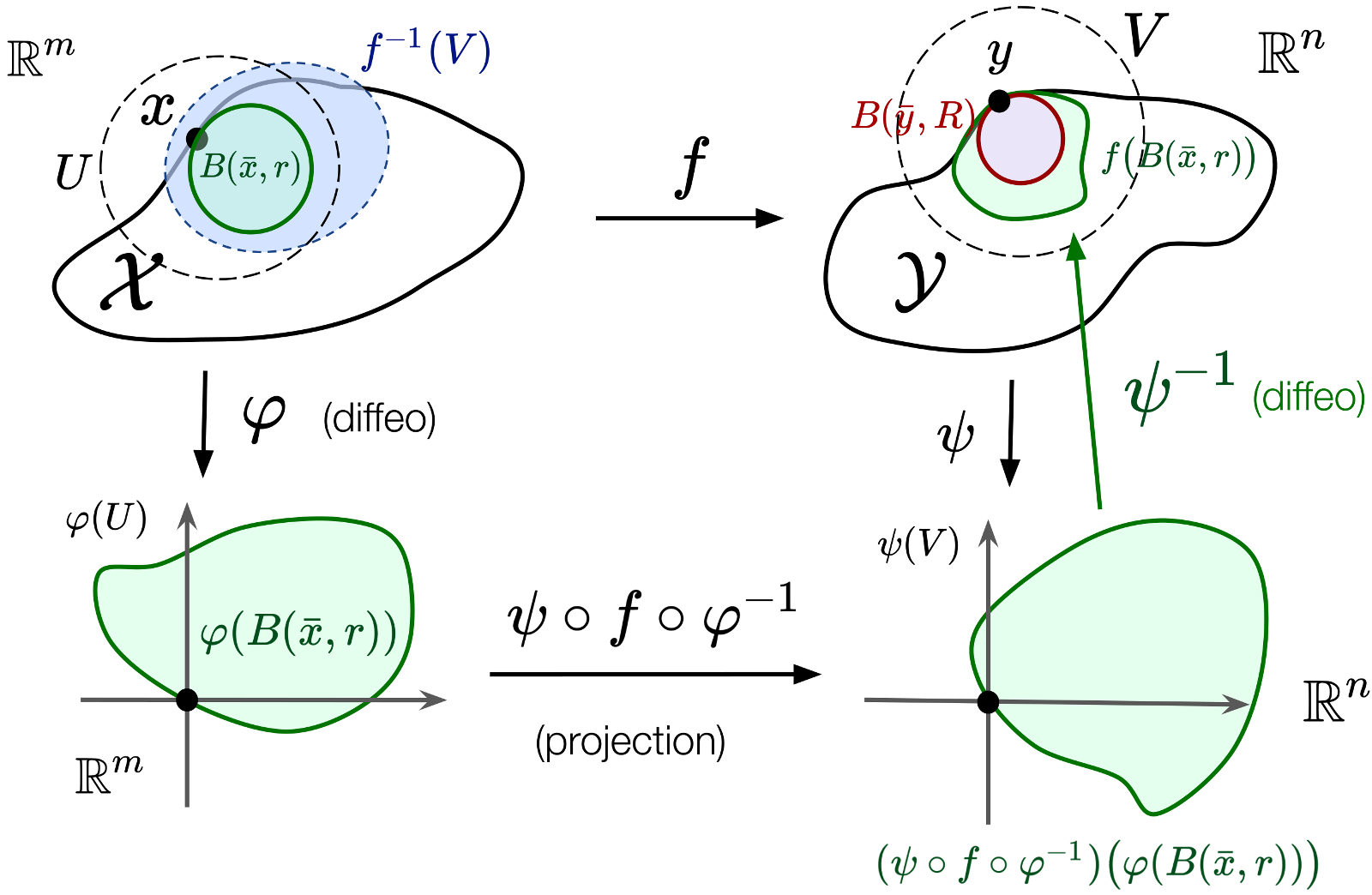
Contributions. We derive new error bounds for reconstructing the convex hull of the image $\mathcal{Y}=f(\mathcal{X})$ of a set $\mathcal{X}$. The set $\mathcal{Y}$ may be non-convex and its boundary may self-intersect. Our results rely on the smoothness of $f$ and of the boundary of $\mathcal{X}$, and on the surjectivity of the differential of $f$, denoted by $\textrm{d}f$. Our main result is stated below.

Theorem 1.1 (Estimation error for the convex hull of $f(\mathcal{X})$).

Let $r,\delta>0$, $\mathcal{X}\subset\mathbb{R}^{m}$ be a non-empty path-connected compact set that is $r$-smooth (see Definition 2.4), $f:\mathbb{R}^{m}\to\mathbb{R}^{n}$, $\mathcal{Y}=f(\mathcal{X})$, and $Z_{\delta}=\{x_{i}\}_{i=1}^{M}\subset\partial\mathcal{X}$ be a $\delta$-cover of the boundary $\partial\mathcal{X}$. If $f$ is a $C^{1}$ submersion such that $(f,\textrm{d}f)$ are $(\bar{L},\bar{H})$-Lipschitz, then

$$d_{H}(\textrm{H}(\mathcal{Y}),\textrm{H}(f(Z_{\delta})))\leq\frac{1}{2}\left(\frac{\bar{L}}{r}+\bar{H}\right)\delta^{2}.$$ (1)

Submersions form a large class of functions of interest, see Section 5 for examples. If we apply this result to the particular case where $\mathcal{X}$ is convex and $f(x)=x$ (so that $\mathcal{Y}=\mathcal{X}$ is convex and $\bar{L}/r+\bar{H}=1/r$), we obtain the bound $d_{H}(\mathcal{X},\textrm{H}(Z_{\delta}))\leq\delta^{2}/(2r)$, which is $2\times$ tighter than the bound in [DW96, Theorem 1], see Section D. We discuss the error bound further in Section 4.3.

Consequences of Theorem 1.1. The derivation of this result is motivated by applications:

1. Geometric inference (Section 5.1): The convex hull of the image $f(\mathcal{X})$ of sets $\mathcal{X}$ with smooth boundary can be accurately approximated using inputs $x_{i}$ sampled from a distribution supported on the boundary of $\mathcal{X}$. Theorem 1.1 gives tighter and more general high-probability error bounds (Corollary 5.2) than prior work [DW96, LJBP22].

2. Robustness analysis of dynamical systems (Section 5.2): Theorem 1.1 justifies approximating convex hulls of reachable sets of dynamical systems from a finite sample (Corollary 5.3). Such sampling-based approaches can be used to quickly verify properties of complex systems (e.g., checking that a dynamical system controlled by a neural network satisfies constraints) but previous error bounds do not explain promising empirical results [LJBP22]. As Theorem 1.1 applies to submersions, it applies to systems with a larger number of uncertain parameters than reachable states (e.g., characterizing the reachable set of a drone transporting a payload of uncertain mass for a given set of initial states).

3. Robust programming (Section 5.3), planning, and control (Section 5.4): The numerical resolution of non-convex optimization problems with constraints that should be satisfied for a range of parameters (e.g., for all parameters in a ball of radius $r$) remains challenging. Theorem 1.1 implies that sampling constraints can yield feasible relaxations of a class of robust programs (Corollary 5.4), with applications to robust planning and controller design (Section 5.4).

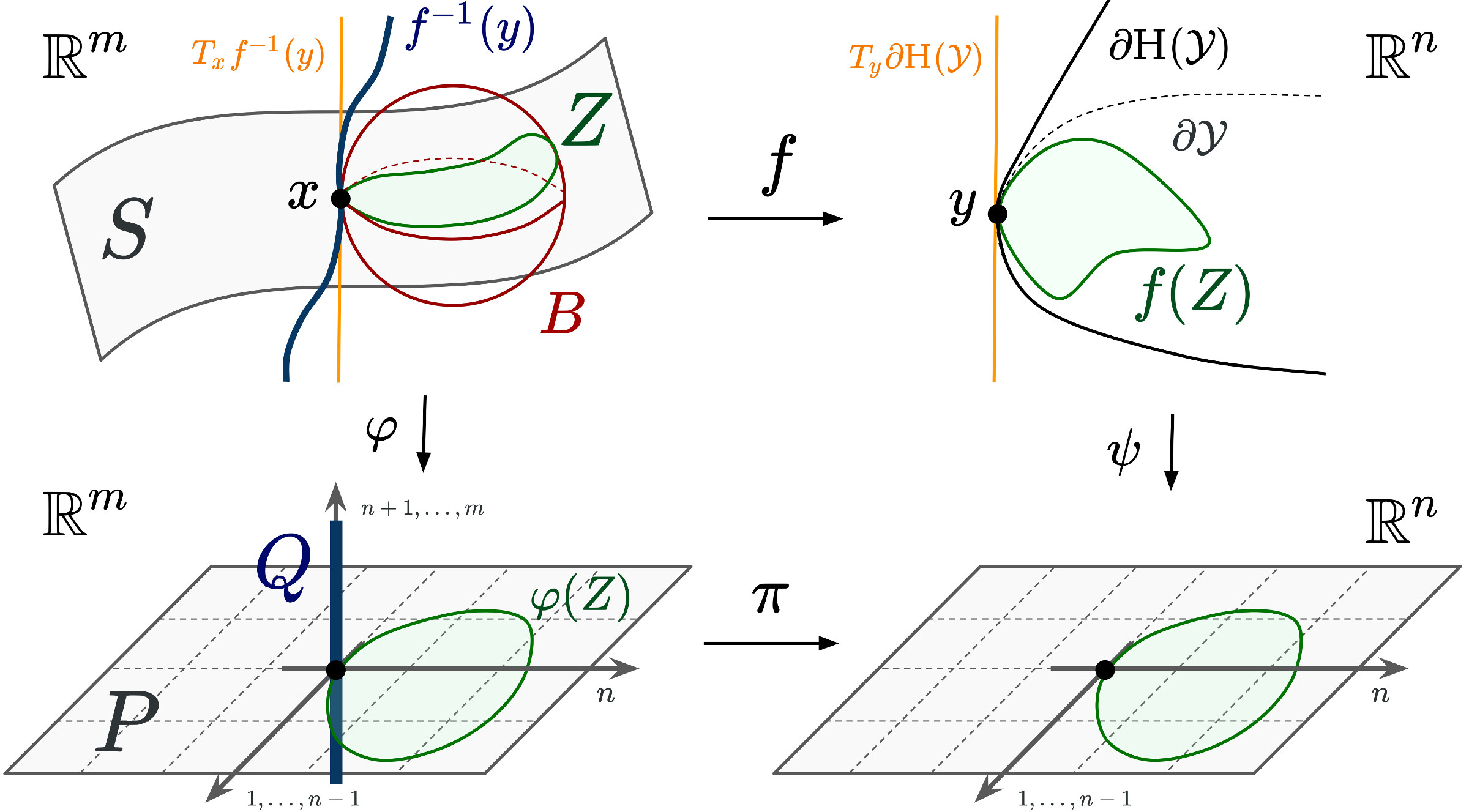
Sketch of proof. To prove Theorem 1.1, we express the approximation error as a function of distances between sampled outputs $f(x_{i})$ and tangent spaces of the boundary of $\textrm{H}(\mathcal{Y})$, and exploit the smoothness of $f$ and of the boundary of $\mathcal{X}$. Deriving this result is complicated by the absence of a smooth manifold structure for the output set boundary $\partial\mathcal{Y}$ that precludes the direct application of tools from differential geometry to $\mathcal{Y}$, since its boundary $\partial\mathcal{Y}$ may self-intersect, see Example 3.1. Our analysis relies on three steps:

1. Proving that the boundary of the convex hull $\textrm{H}(\mathcal{Y})$ is always smooth under our assumptions (Theorem 3.4 and Corollary 3.8). In particular, the boundary $\partial\textrm{H}(\mathcal{Y})$ is an $(n-1)$-dimensional submanifold and the tangent spaces $T_{y}\partial\textrm{H}(\mathcal{Y})$ at points $y\in\partial\textrm{H}(\mathcal{Y})$ are well-defined.

2. Relating bounds on distances to the convex hull tangent spaces $T_{y}\partial\textrm{H}(\mathcal{Y})$ at boundary outputs $y$ to bounds on the Hausdorff distance error of convex hull approximations (Lemma 4.4).

3. Deriving a bound on distances to the tangent spaces $T_{y}\partial\textrm{H}(\mathcal{Y})$ (Lemma 4.5). This bound relies on showing that tangent spaces are mapped to tangent spaces ($\textrm{d}f_{x}(T_{x}\partial\mathcal{X})=T_{y}\partial\textrm{H}(\mathcal{Y})$) for particular choices of inputs $x$ and outputs $y$ using the rank theorem (Lemma 4.7), and subsequently studying images of inputs using the smoothness of $f$ and $\partial\mathcal{X}$ and by decomposing components that are tangential and normal to the tangent spaces $T_{y}\partial\textrm{H}(\mathcal{Y})$.

This approach gives an error bound (Theorem 1.1) that is tighter than a bound more easily derived by assuming that $f$ is a diffeomorphism (Lemma 4.8), which allows exploiting the smoothness of the boundary of $\mathcal{Y}$ (Corollary 3.3) but is a more restrictive assumption, see Section 4.4. It is also tighter than a bound of the form $d_{H}(\textrm{H}(\mathcal{Y}),\textrm{H}(f(Z_{\delta})))\leq\bar{L}\delta$ from a naive covering argument (Lemma 4.2).

The paper is organized as follows. In Section 2, we present notations, different notions of geometric regularity, and review connections between these concepts. In Section 3, we study the structure of the convex hull $\textrm{H}(\mathcal{Y})$. In Section 4, we derive error bounds and prove Theorem 1.1. In Section 5, we provide applications. In Section 6, we conclude and discuss future research directions. For conciseness, the proofs of various intermediate results are provided in the Appendix.

2   Notations and background

Notations. We denote by $a^{\top}b$ the Euclidean inner product of $a,b\in\mathbb{R}^{n}$, by $\|a\|$ the Euclidean norm of $a\in\mathbb{R}^{n}$, by $\mathcal{K}$ the family of non-empty compact subsets of $\mathbb{R}^{n}$, by $\mathcal{B}(\mathbb{R}^{n})$ the Borel $\sigma$-algebra for the Euclidean topology on $\mathbb{R}^{n}$ associated to $\|\cdot\|$, by $\lambda_{n}(\cdot)$ the Lebesgue measure over $\mathbb{R}^{n}$, by $B(x,r)=\{y\in\mathbb{R}^{n}:\|y-x\|\leq r\}$ the closed ball of center $x\in\mathbb{R}^{n}$ and radius $r\geq 0$, and by $\mathring{B}(x,r)$ the open ball. Given $A,B\subset\mathbb{R}^{n}$ and $c\in\mathbb{R}$, we denote by $\textrm{Int}(A)$, $\overline{A}$, $\partial A=\overline{A}\setminus\textrm{Int}(A)$, and $A^{\mathsf{c}}=\mathbb{R}^{n}\setminus A$ the interior, closure, boundary, and complement of $A$, $cA=\{ca:a\in A\}$, by $A+B=\{a+b:a\in A,b\in B\}$ and $A-B=(A^{\mathsf{c}}+(-B))^{\mathsf{c}}$ the Minkowski addition and difference, by $\textrm{H}(A)$ the convex hull of $A$, by $\textrm{Extreme}(A)$ the set of extreme points of $A$, by $d_{A}(x)=\inf_{a\in A}\|x-a\|$ the distance from $x\in\mathbb{R}^{n}$ to $A$, and by $d_{H}(A,B)=\max(\sup_{x\in A}d_{B}(x),\sup_{y\in B}d_{A}(y))$ the Hausdorff distance between $A,B\in\mathcal{K}$.

Differential geometry. Let $\mathcal{M}\subseteq\mathbb{R}^{n}$ be a $k$-dimensional submanifold without boundary. Equipped with the induced metric from the ambient Euclidean norm $\|\cdot\|$, $\mathcal{M}$ is a Riemannian submanifold. The geodesic distance on $\mathcal{M}$ between $x,y\in\mathcal{M}$ is denoted by $d^{\mathcal{M}}(x,y)$. For any $p\in\mathcal{M}$, $T_{p}\mathcal{M}$ and $N_{p}\mathcal{M}$ denote the tangent and normal spaces of $\mathcal{M}$[Lee12], respectively, which we view as linear subspaces of $\mathbb{R}^{n}$. For any $p\in\mathcal{M}$, the second fundamental form of $\mathcal{M}$ is denoted as $\mathrm{II}^{\mathcal{M}}_{p}:T_{p}\mathcal{M}\times T_{p}\mathcal{M}\to N_{p}\mathcal{M}$ and describes the curvature of $\mathcal{M}$ [Lee18].

Given a map $f:\mathbb{R}^{m}\to\mathbb{R}^{n}$ and $x,v,w\in\mathbb{R}^{n}$, $\textrm{d}f_{x}$ and $\textrm{d}^{2}f_{x}$ denote the first- and second-order differentials of $f$ at $x$, with $\textrm{d}f_{x}(v)=\sum_{i=1}^{m}\frac{\partial f}{\partial x_{i}}(x)v_{i}$ and $\textrm{d}^{2}f_{x}(v,w)=\sum_{i=1}^{m}\sum_{j=1}^{m}\frac{\partial^{2}f}{\partial x_{i}\partial x_{j}}(x)v_{i}w_{j}$, and $\textrm{Ker}(\textrm{d}f_{x})=\{v\in T_{x}\mathbb{R}^{m}:\textrm{d}f_{x}(v)=0\}$ denotes the kernel of $\textrm{d}f_{x}$. A differentiable map $f$ is a submersion if $\textrm{d}f_{x}:T_{x}\mathbb{R}^{m}\to T_{f(x)}\mathbb{R}^{n}$ is surjective for all $x\in\mathbb{R}^{m}$, and a diffeomorphism if it is a bijection and its inverse is differentiable.

2.1   Geometric regularity: reach, $R$-convexity, rolling balls, and $R$-smoothness

We introduce different important notions of geometric smoothness.

Definition 2.1 (Reach).

The reach of a closed set $\mathcal{X}\subset\mathbb{R}^{n}$ is defined as

$$\textrm{reach}(\mathcal{X})=\inf_{x\in\mathcal{X}}d(x,\text{Med}(\mathcal{X})),$$

where the medial axis of $\mathcal{X}$, denoted as $\text{Med}(\mathcal{X})$, is the set of points that have at least two nearest neighbors on $\mathcal{X}$.

For a convex set $\mathcal{X}$, $\text{Med}(\mathcal{X})=\emptyset$ and $\textrm{reach}(\mathcal{X})=\infty$.

Definition 2.2 ($R$-convexity).

Let $R>0$ and $\mathcal{X}\subset\mathbb{R}^{n}$. We say that $\mathcal{X}$ is $R$-convex if $\mathcal{X}=\bigcap_{\{\mathring{B}(x,R):\,\mathring{B}(x,R)\cap\mathcal{X}=\emptyset\}}\left(\mathring{B}(x,R))\right)^{\mathsf{c}}$.

Definition 2.3 (Rolling ball).

Let $R>0$ and $\mathcal{X}\subset\mathbb{R}^{n}$ be a non-empty closed set. We say that a ball of radius $R$ rolls freely in $\mathcal{X}$ if for any $x\in\partial\mathcal{X}$, there exists $a\in\mathcal{X}$ such that $x\in B(a,R)\subseteq\mathcal{X}$.

Figure 1: Reach and medial axis.

Figure 2: A ball of radius $R$ rolls freely in $\mathcal{X}$ and in $\overline{\mathcal{X}^{\mathsf{c}}}$.

Definition 2.4 ($R$-smooth set).

Let $R\geq 0$ and $\mathcal{X}\subset\mathbb{R}^{n}$ be a non-empty closed set. We say that $\mathcal{X}$ is $R$-smooth if a ball of radius $R$ rolls freely in $\mathcal{X}$ and in $\overline{\mathcal{X}^{\mathsf{c}}}$. Specifically, for any $x\in\partial\mathcal{X}$, there exists $a\in\mathcal{X}$ and $\bar{a}\in\overline{\mathcal{X}^{\mathsf{c}}}$ such that $x\in B(a,R)\subseteq\mathcal{X}$ and $x\in B(\bar{a},R)\subseteq\overline{\mathcal{X}^{\mathsf{c}}}$

A submanifold $\mathcal{M}\subset\mathbb{R}^{n}$ of reach $R>0$ has a curvature bounded by $1/R$ (Lemma 2.6) and a tubular neighborhood [Lee18] of radius $R$. A set $\mathcal{X}$ is $R$-convex if it is the intersection of complements of balls of radius $R$ [Cue09]. Thus, $R$-convexity generalizes the notion of convexity, since convex sets $\mathcal{X}$ can be expressed as intersections of halfspaces containing $\mathcal{X}$. The rolling ball condition [Wal97, Wal99] is an intuitive notion that we use to define $R$-smooth sets $\mathcal{X}$, for which it is possible to roll a ball of radius $R$ both inside and outside $\mathcal{X}$. We will use these four different concepts to derive error bounds.

2.2   Equivalences and connections between definitions

A key result is the following generalization of Blaschke’s Rolling Theorem [Wal99].

Theorem 2.1.

[Wal99] Let $\mathcal{X}\subset\mathbb{R}^{n}$ be a non-empty path-connected compact set and $R>0$. Then, the following are equivalent:

1. $\mathcal{X}=(\mathcal{X}+B(0,\lambda))-B(0,\lambda)$ for all $\lambda\in[0,R)$ and $\mathcal{X}=(\mathcal{X}-B(0,\lambda))+B(0,\lambda)$ for all $\lambda\in[0,R]$.

2. $\mathcal{X}$ and $\overline{\mathcal{X}^{\mathsf{c}}}$ are $R$-convex and $\textrm{Int}(\mathcal{X})\neq\emptyset$.

3. $\mathcal{X}$ is $\lambda$-smooth for all $0\leq\lambda\leq R$.

4. $\partial\mathcal{X}$ is a $(n-1)$-dimensional submanifold in $\mathbb{R}^{n}$ with the outward-pointing unit-norm normal $n(x)$ at $x\in\partial\mathcal{X}$ satisfying $\|n(x)-n(y)\|\leq\frac{1}{R}\|x-y\|$ for all $x,y\in\partial\mathcal{X}$.

The path-connectedness assumption on $\mathcal{X}$ can be replaced by assumptions on path-connected components of $\mathcal{X}$, see [Wal97]; we do not study such extensions in this work.

The next lemmas gather known results in the literature that are used in our subsequent proofs. Results that are not cited are not explicitly stated in the literature and are proved in Section A.

Lemma 2.2.

[PL08, Lemmas A.0.6 and A.0.7] Let $\mathcal{X}\subset\mathbb{R}^{n}$ be a non-empty closed set and $R>0$. Assume that $\mathcal{X}$ is $R$-smooth. Then, $\textrm{reach}(\mathcal{X})\geq R$, $\textrm{reach}(\overline{\mathcal{X}^{\mathsf{c}}})\geq R$, and $\textrm{reach}(\partial\mathcal{X})\geq R$.

Lemma 2.3.

Let $\mathcal{X}\subset\mathbb{R}^{n}$ be a closed set with $\textrm{reach}(\mathcal{X})\geq R>0$. Then, $\mathcal{X}$ is $R$-convex.

Lemma 2.3 corresponds to [CFPL12, Proposition 1], which assumes that $\mathcal{X}$ is compact. Notably, boundedness of $\mathcal{X}$ is not used in the proof of the result, see Section A.

Lemma 2.4.

Let $R>0$ and $\mathcal{X}\subset\mathbb{R}^{n}$ be a non-empty closed set. If $\mathcal{X}$ is $R$-smooth, then $\mathcal{X}$ is $\lambda$-smooth for all $0\leq\lambda\leq R$.

Lemma 2.5.

Let $\mathcal{X}\subset\mathbb{R}^{n}$ be a non-empty convex closed set. Then, a ball rolls freely in $\overline{\mathcal{X}^{\mathsf{c}}}$.

Lemma 2.6.

[NSW08, Proposition 6.1][Aam17, Proposition III.22] Let $\mathcal{M}\subset\mathbb{R}^{n}$ be a submanifold with $\textrm{reach}(\mathcal{M})\geq R>0$. Then, $\|\mathrm{II}_{x}^{\mathcal{M}}(v,v)\|\leq\frac{1}{R}$ for all $x\in\mathcal{M}$ and unit-norm $v\in T_{x}\mathcal{M}$.

The next important result is an alternative characterization of the reach of a set.

Theorem 2.7.

[Fed59, Theorem 4.18] Let $\mathcal{M}\subset\mathbb{R}^{n}$ be a submanifold and $0<r<\infty$. Then, $\textrm{reach}(\mathcal{M})\geq r$ if and only if $d_{T_{p}\mathcal{M}}(q-p)\leq\frac{\|q-p\|^{2}}{2r}$ for all $p,q\in\mathcal{M}$. Thus,

$$\textrm{reach}(\mathcal{M})=\inf_{p\neq q\in\mathcal{M}}\frac{\|q-p\|^{2}}{2d_{T_{p}\mathcal{M}}(q-p)}.$$

Theorem 2.7 provides an alternative definition of the reach of a submanifold, as well as a bound on the distance to the tangent space. We note that [Fed59, Theorem 4.18] applies to closed sets $\mathcal{M}$ that are not necessarily submanifolds, after appropriately defining the tangent space $T_{p}\mathcal{M}$. If $\mathcal{M}$ is a submanifold, the definition of the tangent space in [Fed59, Theorem 4.18] matches the usual definition, see [Fed59, Remark 4.6]. We only apply Theorem 2.7 to submanifolds in this work.

3   Smoothness of the convex hull $\textrm{H}(\mathcal{Y})$

As we will see in Section 4, a set that is $R$-smooth can be accurately reconstructed from a sample. Thus, in this section, we assume that $\mathcal{X}$ is $r$-smooth and study the smoothness properties of the convex hull of $\mathcal{Y}$. The main result of this section is that the convex hull of $\mathcal{Y}$ is always $R$-smooth if $f$ is a submersion (Theorem 3.4) so the boundary of the convex hull is necessarily a submanifold (Corollary 3.8). First, we observe that the convex hull operation preserves smoothness properties.

Lemma 3.1 ($R$-smoothness is preserved after taking the convex hull).

Let $R>0$ and $\mathcal{Y}\subset\mathbb{R}^{n}$ be a non-empty compact set. Assume that $\mathcal{Y}$ is $R$-smooth. Then, $\textrm{H}(\mathcal{Y})$ is $R$-smooth.

Proof.

Since $\textrm{H}(\mathcal{Y})$ is convex, a ball of radius $R$ rolls freely in $\overline{\textrm{H}(\mathcal{Y})^{\mathsf{c}}}$ by Lemma 2.5. Next, we show that a ball of radius $R$ rolls freely inside $\textrm{H}(\mathcal{Y})$.

To do so, we decompose the boundary $\partial\textrm{H}(\mathcal{Y})$ as the disjoint union

$$\partial\textrm{H}(\mathcal{Y})=(\partial\textrm{H}(\mathcal{Y})\setminus\partial\textrm{H}(\mathcal{Y})\cap\partial\mathcal{Y})\cup(\partial\textrm{H}(\mathcal{Y})\cap\partial\mathcal{Y})$$

and study boundary points on these two subsets. We represent this decomposition in Figure 3.

• First, let $y\in\partial\textrm{H}(\mathcal{Y})\cap\partial\mathcal{Y}$. Since $\mathcal{Y}$ is $R$-smooth, there exists a ball $B(\bar{y},R)$ such that $y\in B(\bar{y},R)\subseteq\mathcal{Y}\subseteq\textrm{H}(\mathcal{Y})$.

Figure 3: Decomposition of the boundary of $\textrm{H}(\mathcal{Y})$.

• Second, let $y\in\partial\textrm{H}(\mathcal{Y})\setminus\partial\textrm{H}(\mathcal{Y})\cap\partial\mathcal{Y}$. Then, $y$ lies between two distinct extreme points $y_{1},y_{2}\in\partial\textrm{H}(\mathcal{Y})\cap\partial\mathcal{Y}$, such that $y=ty_{1}+(1-t)y_{2}$ for some $t\in(0,1)$, see Figure 4 (note that $\textrm{H}(\mathcal{Y})=\textrm{H}(\textrm{Extreme}(\mathcal{Y}))=\textrm{H}(\textrm{Extreme}(\partial\mathcal{Y}))$ by the Krein-Milman theorem [Gro73] since $\mathcal{Y}$ is compact, so that $y_{1},y_{2}\in\partial\mathcal{Y}$).

  Since $\mathcal{Y}$ is $R$-smooth, there exist two balls $B(\bar{y}_{1},R)$ and $B(\bar{y}_{2},R)$ satisfying $y_{1}\in B(\bar{y}_{1},R)\subseteq\mathcal{Y}\subseteq\textrm{H}(\mathcal{Y})$ and $y_{2}\in B(\bar{y}_{2},R)\subseteq\mathcal{Y}\subseteq\textrm{H}(\mathcal{Y})$. Define $\bar{y}=t\bar{y}_{1}+(1-t)\bar{y_{2}}$. Then, the ball $B(\bar{y},R)$ satisfies $y\in B(\bar{y},R)\subseteq\textrm{H}(\mathcal{Y})$, since $B(\bar{y},R)\subset\textrm{H}(B(\bar{y}_{1},R)\cup B(\bar{y}_{2},R))\subseteq\textrm{H}(\mathcal{Y})$.

Figure 4: Finding a ball tangent to $\partial\textrm{H}(\mathcal{Y})\setminus\partial\textrm{H}(\mathcal{Y})\cap\partial\mathcal{Y}$.

By the last two steps, a ball of radius $R$ rolls freely in $\textrm{H}(\mathcal{Y})$ and in $\overline{\textrm{H}(\mathcal{Y})^{\mathsf{c}}}$. We conclude that $\textrm{H}(\mathcal{Y})$ is $R$-smooth. ∎

However, even if $\mathcal{X}\subset\mathbb{R}^{m}$ is $r$-smooth and $f$ is a local diffeomorphism (in particular, a submersion), $\mathcal{Y}$ may not be $R$-smooth. Indeed, if $\mathcal{Y}$ is $R$-smooth, then $\partial\mathcal{Y}$ must be a $(n-1)$-submanifold by Theorem 2.1. However, this may not be the case due to self-intersections as shown next.

Example 3.1.

Let $L=\{(r,\theta)\in\mathbb{R}^{2}:r=1.5,(-\pi+0.5)\leq\theta\leq(3\pi/2-0.5)\}$ and define the input set and map

$$\mathcal{X}=L+B(0,0.5),\ f:\mathbb{R}^{2}\to\mathbb{R}^{2}:(r,\theta)\mapsto(r\cos(\theta),r\sin(\theta)).$$

One can freely roll a ball of radius $0.5$ inside $\mathcal{X}$ and $\overline{\mathcal{X}^{\mathsf{c}}}$, so $\mathcal{X}$ is $r$-smooth. Moreover, the map $f$ is a local diffeomorphism on $\mathcal{X}$ (hence a submersion). However, one cannot roll a ball outside $\mathcal{Y}$, so $\mathcal{Y}$ is not $R$-smooth for any $R>0$. We represent $\mathcal{Y}$ in Figure 5.

Figure 5: The boundary of images of sets with smooth boundary can self-intersect.

If $f$ is a diffeomorphism, the output set $\mathcal{Y}$ is always $R$-smooth if $\mathcal{X}$ is $r$-smooth (Corollary 3.3). This result almost immediately follows from the well-known result that the reach is conserved under diffeomorphisms, see [Fed59, Theorem 4.19] and [Aam17, Lemma III.17].

Lemma 3.2 (Stability of the reach under diffeomorphisms).

[Fed59, Theorem 4.19] Let $\mathcal{X}\subset\mathbb{R}^{n}$ be a closed set, $f:\mathbb{R}^{n}\to\mathbb{R}^{n}$, and $\mathcal{Y}=f(\mathcal{X})$. Let $r,s>0$, and assume that $\textrm{reach}(\mathcal{X})\geq r>0$ and that $f|_{\mathcal{X}+B(0,s)}$ is a $C^{1}$ diffeomorphism such that $(f,f^{-1},\textrm{d}f)$ are $(\bar{L},\underline{L},\bar{H})$-Lipschitz, respectively. Then, $$\textrm{reach}(\mathcal{Y})\geq\min\left(\frac{s}{\underline{L}},\frac{1}{\left(\frac{\bar{L}}{r}+\bar{H}\right)\underline{L}^{2}}\right).$$     Figure 6: Positive reach is conserved under diffeomorphisms.

Corollary 3.3 ($r$-smoothness is preserved under diffeomorphisms).

Let $r>0$, $\mathcal{X}\subset\mathbb{R}^{n}$ be a non-empty path-connected $r$-smooth compact set, and $f:\mathbb{R}^{n}\to\mathbb{R}^{n}$ be a $C^{1}$ diffeomorphism such that $(f,f^{-1},\textrm{d}f)$ are $(\bar{L},\underline{L},\bar{H})$-Lipschitz. Let $R^{-1}=\left(\frac{\bar{L}}{r}+\bar{H}\right)\underline{L}^{2}$ and $\mathcal{Y}=f(\mathcal{X})$.

Then, $\mathcal{Y}$ and $\textrm{H}(\mathcal{Y})$ are $R$-smooth, and the boundaries $\partial\mathcal{Y}$ and $\partial\textrm{H}(\mathcal{Y})$ are submanifolds of dimension $(n-1)$ with outward-pointing unit-norm normals that are $(1/R)$-Lipschitz.

Proof.

By Lemma 2.2, $\textrm{reach}(\mathcal{X})\geq r$ and $\textrm{reach}(\overline{\mathcal{X}^{\mathsf{c}}})\geq r$. By Lemma 3.2 $\textrm{reach}(\mathcal{Y})\geq R$ and $\textrm{reach}(\overline{\mathcal{Y}^{\mathsf{c}}})\geq R$. By Lemma 2.3, $\mathcal{Y}$ and $\overline{\mathcal{Y}^{\mathsf{c}}}$ are $R$-convex. Thus, $\mathcal{Y}$ is $R$-smooth by Theorem 2.1 ($\mathcal{Y}$ is a non-empty path-connected compact set since $\mathcal{X}$ is one and $f$ is a diffeomorphism). By applying Lemma 3.1, $\textrm{H}(\mathcal{Y})$ is also $R$-smooth. The last result follows from Theorem 2.1. ∎

However, assuming that $f$ is a diffeomorphism is restrictive, as it implies that $f$ maps between two sets of the same dimension and thus does not allow considering problems with more inputs $x\in\mathcal{X}$ than outputs $y\in\mathcal{Y}$. Although $\mathcal{Y}$ is not necessarily $R$-smooth (see Example 3.1), we show that $\textrm{H}(\mathcal{Y})$ is always $R$-smooth if $f$ is a submersion and $\mathcal{X}$ is $r$-smooth. The result combines Corollary 3.3, the rank theorem, and the decomposition of the convex hull boundary of Lemma 3.1.

Theorem 3.4.

Let $r>0$, $\mathcal{X}\subset\mathbb{R}^{m}$ be a non-empty $r$-smooth compact set, $f:\mathbb{R}^{m}\to\mathbb{R}^{n}$ be a $C^{1}$ submersion, and $\mathcal{Y}=f(\mathcal{X})$. Then, $\textrm{H}(\mathcal{Y})$ is $R$-smooth for some $R>0$.

Theorem 3.4 implies that a ball of radius $R$ rolls freely inside $\textrm{H}(\mathcal{Y})$ and $\overline{\textrm{H}(\mathcal{Y})^{\mathsf{c}}}$ if $f$ is a submersion. To prove Theorem 3.4, we need the following intermediate results.

Lemma 3.5.

[Lee12, Corollary C.36] Let $f:\mathbb{R}^{m}\to\mathbb{R}^{n}$ be a $C^{1}$ submersion. Then, $f$ is an open map.

Lemma 3.6.

Let $f:\mathbb{R}^{m}\to\mathbb{R}^{n}$ be a continuous open map and $\mathcal{X}\subset\mathbb{R}^{m}$ be compact. Then, $\partial f(\mathcal{X})\subseteq f(\partial\mathcal{X})$.

Proof.

$A$ is closed, so $\partial A=\overline{A}\setminus\textrm{Int}(A)=A\setminus\textrm{Int}(A)$ and $A=\textrm{Int}(A)\sqcup\partial A$, where $\sqcup$ denotes the disjoint union. Similarly, $f$ is continuous and $A$ is compact so $f(A)$ is compact and $f(A)=\textrm{Int}(f(A))\sqcup\partial f(A)$. Next, we show that $\partial f(A)\subseteq f(\partial A)$.

Let $x\in\partial f(A)$. Since $\partial f(A)=f(A)\setminus\textrm{Int}(f(A))$, there exists $a\in A$ such that $x=f(a)$ and either $a\in\textrm{Int}(A)$ or $a\in\partial A$. By contradiction, assume that $a\in\textrm{Int}(A)$. Since $f$ is open, $f(\textrm{Int}(A))=\textrm{Int}(f(A))$ so $f(a)\in\textrm{Int}(f(A))$. Since $f(A)=\textrm{Int}(f(A))\sqcup\partial f(A)$, this implies that $x=f(a)\notin\partial f(A)$. This is a contradiction. ∎

Lemma 3.7.

Let $r>0$, $A\subset\mathbb{R}^{m}$ be a non-empty $r$-smooth compact set, and $\pi:\mathbb{R}^{m}\to\mathbb{R}^{n}:(x_{1},\dots,x_{n},x_{n+1},\dots,x_{m})\mapsto(x_{1},\dots,x_{n})$ be the standard projection.

Then, $\pi(A)$ is a non-empty $r$-smooth compact set.

Proof.

$\pi(A)$ is compact since $A$ is compact and $\pi$ is continuous. Next, we show that $\pi(A)$ is $r$-smooth.

Let $y\in\partial\pi(A)$. By Lemma 3.6, $\partial\pi(A)\subseteq\pi(\partial A)$. Thus, there exists $x\in\partial A$ such that $y=\pi(x)$. Since $A$ is $r$-smooth, there exists a ball $B^{m}\triangleq B(\hat{x},r)$ such that $x\in B^{m}\subseteq A$. We easily verify that $B^{n}\triangleq\pi(B^{m})$ with $B^{n}=B(\hat{y},r)=B(\pi(\hat{x}),r)\subset\mathbb{R}^{n}$ satisfies $y\in B^{n}\subseteq\pi(A)$.

Thus, a ball of radius $r$ rolls along $\partial\pi(A)$ inside $\pi(A)$. With minor adaptations, we can show that a ball of radius $r$ rolls along $\partial\pi(A)$ outside $\pi(A)$. We conclude that $\pi(A)$ is $r$-smooth. ∎

Proof of Theorem 3.4.

For any $R>0$, by Lemma 2.5, a ball of radius $R$ rolls freely inside $\overline{\textrm{H}(\mathcal{Y})^{\mathsf{c}}}$, since $\textrm{H}(\mathcal{Y})$ is convex. To conclude, we prove that a ball of radius $R>0$ rolls freely in $\mathcal{Y}$, which implies that a ball of radius $R$ rolls freely in $\textrm{H}(\mathcal{Y})$ (see the proof of Lemma 3.1).

Let $x\in\partial\mathcal{X}$. By the rank theorem, since $f$ is a submersion, there exist two charts $(U_{x},\varphi_{x})$ and $(V_{f(x)},\psi_{f(x)})$ such that $\psi_{f(x)}\circ f\circ\varphi_{x}^{-1}$ is a coordinate projection:

$$\psi_{f(x)}\circ f\circ\varphi_{x}^{-1}:\varphi_{x}(U_{x}\cap f^{-1}(V_{f(x)}))\to\psi_{f(x)}(V_{f(x)}):\hat{x}=(\hat{x}_{1},\dots,\hat{x}_{n},\hat{x}_{n+1},\dots\hat{x}_{m})\mapsto(\hat{x}_{1},\dots,\hat{x}_{n}).$$

Figure 7: Definitions for the proof of Theorem 3.4.

We proceed in three steps.

• Step 1: Build a suitable finite family of charts for $\partial\mathcal{X}$. Since $\mathcal{X}$ is $r$-smooth, $\mathcal{X}$ is $\lambda$-smooth for all $0\leq\lambda\leq r$ by Lemma 2.4. Thus, for any $0<r_{x}\leq r$ and any $\tilde{x}\in\partial\mathcal{X}\cap U_{x}$, there is a ball $B(\bar{x},r_{x})$ such that $\tilde{x}\in B(\bar{x},r_{x})\subseteq\mathcal{X}$. Let $\epsilon_{x}>0$ be small-enough so that $B(x,\epsilon_{x})\subset U_{x}$. Then, by choosing $r_{x}>0$ small-enough,

  $$(P)\quad\text{for any }\tilde{x}\in\partial\mathcal{X}\cap B(x,\epsilon_{x}),\ \text{there is }B(\bar{x},r_{x})\ \text{such that }\tilde{x}\in B(\bar{x},r_{x})\subset\mathcal{X}\cap U_{x}.$$

  The family $\{(B(x,\epsilon_{x}),\varphi_{x})\}_{x\in\partial\mathcal{X}}$ is thus a family of smooth charts that covers $\partial\mathcal{X}$ and satisfies (P). Since $\partial\mathcal{X}$ is compact, there exists a finite subcover of $\{(B(x,\epsilon_{x}),\varphi_{x})\}_{x\in\partial\mathcal{X}}$. Thus, we restrict our attention to a finite family of such charts $\{(B(x_{i},\epsilon_{x_{i}}),\varphi_{x_{i}})\}_{i\in I}$ covering $\partial\mathcal{X}$ satisfying (P).

• Step 2: Show that there is a ball at any $y\in\partial\mathcal{Y}$ inside $\mathcal{Y}$. Let $y\in\partial\mathcal{Y}$ be arbitrary and $\tilde{x}\in\partial\mathcal{X}$ be such that $y=f(\tilde{x})$ (this $\tilde{x}$ exists since $\partial\mathcal{Y}\subseteq f(\partial\mathcal{X})$, by Lemmas 3.5 and 3.6 since $f$ is a submersion). Then, since the $B(x_{i},\epsilon_{x_{i}})$ cover $\partial\mathcal{X}$, $\tilde{x}$ is in the domain of one of the charts $(B(x_{i},\epsilon_{x_{i}}),\varphi_{x_{i}})$ for some $i\in I$, i.e., $\tilde{x}\in\partial\mathcal{X}\cap B(x_{i},\epsilon_{x_{i}})$. Thus, by (P), there exists $B(\bar{x},r_{x_{i}})$ such that $\tilde{x}\in B(\bar{x},r_{x_{i}})\subset\mathcal{X}\cap U_{x_{i}}$. Next, we prove that $f(B(\bar{x},r_{x_{i}}))$ is $R_{x_{i}}$-smooth for some $R_{x_{i}}>0$ in four steps. For conciseness, we denote $\varphi=\varphi_{x_{i}}$ and $\psi=\psi_{f(x_{i})}$.

  • $B(\bar{x},r_{x_{i}})$ is $r_{x_{i}}$-smooth.

  • By Corollary 3.3, $\varphi(B(\bar{x},r_{x_{i}}))$ is $\tilde{r}_{x_{i}}$-smooth for some $\tilde{r}_{x_{i}}>0$, since $B(\bar{x},r_{x_{i}})$ is $r_{x_{i}}$-smooth and $\varphi$ is a diffeomorphism on $U_{x_{i}}$ with $B(\bar{x},r_{x_{i}})\subset U_{x_{i}}$.

  • By Lemma 3.7, $(\psi\circ f)(B(\bar{x},r_{x_{i}}))$ is $\tilde{r}_{x_{i}}$-smooth, since $(\psi\circ f)(B(\bar{x},r_{x_{i}}))=(\psi\circ f\circ\varphi^{-1})(\varphi(B(\bar{x},r_{x_{i}})))=\pi(\varphi(B(\bar{x},r_{x_{i}})))$ and $\varphi(B(\bar{x},r_{x_{i}}))$ is $\tilde{r}_{x_{i}}$-smooth.

  • By Corollary 3.3, $f(B(\bar{x},r_{x_{i}}))$ is $R_{x_{i}}$-smooth for some $R_{x_{i}}>0$, since $(\psi\circ f)(B(\bar{x},r_{x_{i}}))$ is $\tilde{r}_{x_{i}}$-smooth and $\psi^{-1}$ is a diffeomorphism.

  Since $f(B(\bar{x},r_{x_{i}}))$ is $R_{x_{i}}$-smooth and $y\in\partial f(B(\bar{x},r_{x_{i}}))$, for any $0<R\leq R_{x_{i}}$, there exists a ball $B(\bar{y},R)$ such that $y\in B(\bar{y},R)\subseteq f(B(\bar{x},r_{x_{i}}))\subseteq\mathcal{Y}$.

• Step 3: Show that there is a ball of fixed radius $R$ at any $y\in\partial\mathcal{Y}$ inside $\mathcal{Y}$. Let $R=\inf_{i\in I}R_{x_{i}}$. Since $R_{x_{i}}>0$ for all $i\in I$ and $I$ is finite, $R>0$. Since $0<R\leq R_{x_{i}}$ for all $i\in I$, we apply Step 2 and obtain that for any $y\in\partial\mathcal{Y}$, there exists a ball $B(\bar{y},R)$ such that $y\in B(\bar{y},R)\subseteq\mathcal{Y}$.

Thus, a ball of radius $R$ rolls freely in $\mathcal{Y}$ for some $R>0$. This concludes the proof. ∎

We stress that Theorem 3.4 does not imply that $\mathcal{Y}$ is $R$-smooth, as $\mathcal{Y}$ may self-intersect, see Example 3.1. The main idea of the proof is that intersections disappear after taking the convex hull.

Corollary 3.8.

Let $r>0$, $\mathcal{X}\subset\mathbb{R}^{m}$ be a non-empty $r$-smooth compact set, $f:\mathbb{R}^{m}\to\mathbb{R}^{n}$ be a $C^{1}$ submersion, and $\mathcal{Y}=f(\mathcal{X})$. Then, $\partial\textrm{H}(\mathcal{Y})$ is a submanifold of dimension $(n-1)$.

Proof.

$\textrm{H}(\mathcal{Y})$ is $R$-smooth for some $R>0$ by Theorem 3.4. Since $\textrm{H}(\mathcal{Y})$ is always path-connected since it is convex, the conclusion follows from Theorem 2.1. ∎

Albeit $\textrm{H}(\mathcal{Y})$ is $R$-smooth, the constant $R>0$ in Theorem 3.4 depends on the smoothness of local charts given by the rank theorem. These smoothness constants are difficult to characterize. The error bounds we derive in Theorem 1.1 are independent of this constant. Nevertheless, the fact that $\partial\textrm{H}(\mathcal{Y})$ is a $(n-1)$-dimensional submanifold will be essential to our later derivations.

4   Error bounds

In this section, we derive error bounds for the reconstruction of the convex hull of $\mathcal{Y}=f(\mathcal{X})$ from a sample and prove Theorem 1.1. In Section 4.1, as a baseline, we first derive a coarse error bound using a standard $\delta$-covering argument. In Section 4.2, we derive tighter error bounds that exploit the smoothness of the boundary $\partial\textrm{H}(\mathcal{Y})$.

4.1   Naive error bound via covering ($f$ is Lipschitz)

Lemma 4.1 provides sufficient conditions to achieve $\epsilon$-accurate reconstruction of the convex hull.

Lemma 4.1.

Let $\epsilon\geq 0$, $A,\mathcal{Y}\in\mathcal{K}$ satisfy $\partial\mathcal{Y}\subseteq A+B(0,\epsilon)$ and $A\subseteq\mathcal{Y}$. Then, $d_{H}(\textrm{H}(\mathcal{Y}),\textrm{H}(A))\leq\epsilon$.

Proof.

An equivalent definition of the Hausdorff distance is $d_{H}(\textrm{H}(\mathcal{Y}),\textrm{H}(A))=\min\{\epsilon\geq 0:\textrm{H}(\mathcal{Y})\subseteq\textrm{H}(A)+B(0,\epsilon),\textrm{H}(A)\subseteq\textrm{H}(\mathcal{Y})+B(0,\epsilon)\}$ [Sch14].

$\partial\mathcal{Y}\subseteq A+B(0,\epsilon)$ implies that $\textrm{H}(\mathcal{Y})=\textrm{H}(\partial\mathcal{Y})\subseteq\textrm{H}(A+B(0,\epsilon))=\textrm{H}(A)+B(0,\epsilon)$. $A\subseteq\mathcal{Y}$ implies that $\textrm{H}(A)\subseteq\textrm{H}(\mathcal{Y})\subset\textrm{H}(\mathcal{Y})+B(0,\epsilon)$. Thus, together, $\textrm{H}(\mathcal{Y})\subseteq\textrm{H}(A)+B(0,\epsilon)$ and $\textrm{H}(A)\subseteq\textrm{H}(\mathcal{Y})+B(0,\epsilon)$ imply that $d_{H}(\textrm{H}(A),\textrm{H}(\mathcal{Y}))\leq\epsilon$. ∎

Combined with a standard covering argument, Lemma 4.1 allows deriving an error bound for the convex hull reconstruction from a sample $Z_{\delta}=\{x_{i}\}_{i=1}^{M}$ in $\mathcal{X}$.

Lemma 4.2.

Let $\mathcal{X}\subset\mathbb{R}^{m}$ be a non-empty compact set, $f:\mathbb{R}^{m}\to\mathbb{R}^{n}$ be a $\bar{L}$-Lipschitz function, $\mathcal{Y}=f(\mathcal{X})$, $\delta>0$, and $Z_{\delta}\subset\mathcal{X}$. Assuming that either

• $Z_{\delta}$ is a $\delta$-cover of $\mathcal{X}$ (i.e., $\mathcal{X}\subseteq Z_{\delta}+B(0,\delta)$), or

• $Z_{\delta}$ is a $\delta$-cover of $\partial\mathcal{X}$ (i.e., $\partial\mathcal{X}\subseteq Z_{\delta}+B(0,\delta)$) and $\partial\mathcal{Y}\subseteq f(\partial\mathcal{X})$,

then

$$d_{H}(\textrm{H}(\mathcal{Y}),\textrm{H}(f(Z_{\delta})))\leq\bar{L}\delta.$$

Proof.

In both cases, $f(Z_{\delta})$ is an $(\bar{L}\delta)$-cover of $\partial\mathcal{Y}$. Thus, $\partial\mathcal{Y}\subseteq f(Z_{\delta})+B(0,\bar{L}\delta)$. Also, $f(Z_{\delta})\subseteq\mathcal{Y}$ since $f(Z_{\delta})\subseteq f(\mathcal{X})=\mathcal{Y}$. The conclusion follows from Lemma 4.1 with $A=f(Z_{\delta})$ and $\epsilon=\bar{L}\delta$. ∎

4.2   Error bound via smoothness of the boundary ($f$ is $C^{1}$ and $\mathcal{X}$ is $r$-smooth)

4.2.1 Bound on $d_{T_{y}\partial\textrm{H}(\mathcal{Y})}$ implies bound on Hausdorff distance $d_{H}(\textrm{H}(\mathcal{Y}),\textrm{H}(A))$

In this section, we show that a bound on the distance to the tangent space $T_{y}\partial\textrm{H}(\mathcal{Y})$ gives a Hausdorff distance error bound on the convex hull reconstruction.

Lemma 4.3.

Let $\mathcal{M}\subset\mathbb{R}^{n}$ be a compact submanifold of dimension $(n-1)$, $x\in\mathcal{M}$, and $v\in T_{x}\mathcal{M}$. Denote by $n^{\mathcal{M}}(x)$ the unit-norm outward-pointing normal of $\mathcal{M}$ at $x$, and by $\pi_{x}^{\top}$ and $\pi_{x}^{\perp}$ the linear projection operators onto $T_{x}\mathcal{M}$ and $N_{x}\mathcal{M}$, respectively. Then, $d_{T_{x}\mathcal{M}}(v)=\|\pi_{x}^{\perp}(v)\|=|v^{\top}n^{\mathcal{M}}(x)|$.

Proof.

$d_{T_{x}\mathcal{M}}(v)=\inf_{w\in T_{x}\mathcal{M}}\|v-w\|=\|v-\pi_{x}^{\top}(v)\|$. Then, note that $(v-\pi_{x}^{\top}(v))\in N_{x}\mathcal{M}$ since $\pi_{x}^{\top}(v-\pi_{x}^{\top}(v))=0$ by linearity. Thus, $v-\pi_{x}^{\top}(v)=\pi_{x}^{\perp}(v-\pi_{x}^{\top}(v))$ and we obtain that $d_{T_{x}\mathcal{M}}(v)=\|\pi_{x}^{\perp}(v)\|$. To show that $\|\pi_{x}^{\perp}(v)\|=|v^{\top}n^{\mathcal{M}}(x)|$, we write $T_{x}\mathcal{M}=\{v\in\mathbb{R}^{n}:v^{\top}n^{\mathcal{M}}(x)=0\}$. Then, $\pi^{\top}(v)=v-(v^{\top}n^{\mathcal{M}}(x))n^{\mathcal{M}}(x)$ so $\pi^{\perp}(v)=(v^{\top}n^{\mathcal{M}}(x))n^{\mathcal{M}}(x)$ and the conclusion follows. ∎

Lemma 4.4.

Let $\mathcal{Y},A\subset\mathbb{R}^{n}$ be non-empty compact sets such that $A\subseteq\textrm{H}(\mathcal{Y})$ and $\partial\textrm{H}(\mathcal{Y})$ is a submanifold of dimension $(n-1)$. Then,

$$d_{H}(\textrm{H}(\mathcal{Y}),\textrm{H}(A))\leq\sup_{y\in\partial\textrm{H}(\mathcal{Y})\cap\partial\mathcal{Y}}\left(\operatornamewithlimits{inf\vphantom{p}}_{a\in A}d_{T_{y}\partial\textrm{H}(\mathcal{Y})}(y-a)\right).$$ (2)

Proof.

For any non-empty convex compact set $C\subset\mathbb{R}^{n}$, the support function of $C$ is defined as $h(C,\cdot):\mathbb{R}^{n}\to\mathbb{R},\ u\mapsto h(C,u)=\sup_{y\in C}y^{\top}u$ and is convex and continuous [Sch14]. $\textrm{H}(\mathcal{Y})$ and $\textrm{H}(A)$ are both convex, non-empty, and compact. Thus, by [Sch14, Lemma 1.8.14],

$$d_{H}(\textrm{H}(\mathcal{Y}),\textrm{H}(A)) =\sup_{u\in\partial B(0,1)}|h(\textrm{H}(\mathcal{Y}),u)-h(\textrm{H}(A),u)|=|h(\textrm{H}(\mathcal{Y}),u_{0})-h(\textrm{H}(A),u_{0})|$$

$$=\bigg{|}\sup_{y\in\textrm{H}(\mathcal{Y})}y^{\top}u_{0}-\sup_{q\in\textrm{H}(A)}q^{\top}u_{0}\bigg{|}$$

for some $u_{0}\in\mathbb{R}^{n}$ with $\|u_{0}\|=1$.

Let $y_{0}\in\partial\textrm{H}(\mathcal{Y})$ be such that $h(\textrm{H}(\mathcal{Y}),u_{0})=y_{0}^{\top}u_{0}$, so that $y^{\top}u_{0}\leq y_{0}^{\top}u_{0}$ for all $y\in\textrm{H}(\mathcal{Y})$. Then, $u_{0}=n^{\partial\textrm{H}(\mathcal{Y})}(y_{0})$ [DW96], where $n^{\partial\textrm{H}(\mathcal{Y})}$ denotes the unit-norm outward-pointing normal of $\partial\textrm{H}(\mathcal{Y})$, and $(y_{0}-y)^{\top}n^{\partial\textrm{H}(\mathcal{Y})}(y_{0})\geq 0$ for all $y\in\textrm{H}(\mathcal{Y})$.

Without loss of generality, we may assume that $y_{0}\in\partial\textrm{H}(\mathcal{Y})\cap\partial\mathcal{Y}$. Indeed, if $y_{0}\notin\partial\mathcal{Y}$, then there exists $y_{1}\in\partial\textrm{H}(\mathcal{Y})\cap\partial\mathcal{Y}$ with $(y_{0}-y_{1})^{\top}n^{\partial\textrm{H}(\mathcal{Y})}(y_{0})=0$. Thus, for some $y_{0}\in\partial\textrm{H}(\mathcal{Y})\cap\partial\mathcal{Y}$,

$$d_{H}(\textrm{H}(\mathcal{Y}),\textrm{H}(A)) =\bigg{|}y_{0}^{\top}n^{\partial\textrm{H}(\mathcal{Y})}(y_{0})-\sup_{q\in\textrm{H}(A)}q^{\top}n^{\partial\textrm{H}(\mathcal{Y})}(y_{0})\bigg{|}=\bigg{|}\inf_{q\in\textrm{H}(A)}(y_{0}-q)^{\top}n^{\partial\textrm{H}(\mathcal{Y})}(y_{0})\bigg{|}$$

$$=\inf_{q\in\textrm{H}(A)}(y_{0}-q)^{\top}n^{\partial\textrm{H}(\mathcal{Y})}(y_{0})$$

since $(y_{0}-q)^{\top}n^{\partial\textrm{H}(\mathcal{Y})}(y_{0})\geq 0$ for all $q\in\textrm{H}(A)$ because $\textrm{H}(A)\subseteq\textrm{H}(\mathcal{Y})$.

$\inf_{q\in\textrm{H}(A)}(y_{0}-q)^{\top}n^{\partial\textrm{H}(\mathcal{Y})}(y_{0})$ amounts to minimizing a linear function over a convex domain. Thus, $\inf_{q\in\textrm{H}(A)}(y_{0}-q)^{\top}n^{\partial\textrm{H}(\mathcal{Y})}(y_{0})=\inf_{a\in A}(y_{0}-a)^{\top}n^{\partial\textrm{H}(\mathcal{Y})}(y_{0})$ and

$$d_{H}(\textrm{H}(\mathcal{Y}),\textrm{H}(A)) =\inf_{a\in A}(y_{0}-a)^{\top}n^{\partial\textrm{H}(\mathcal{Y})}(y_{0}).$$

Since $(y_{0}-a)^{\top}n^{\partial\textrm{H}(\mathcal{Y})}(y_{0})\geq 0$ for all $a\in A$ because $A\subseteq\textrm{H}(\mathcal{Y})$, we obtain

$$d_{H}(\textrm{H}(\mathcal{Y}),\textrm{H}(A)) =\inf_{a\in A}(y_{0}-a)^{\top}n^{\partial\textrm{H}(\mathcal{Y})}(y_{0})=\inf_{a\in A}\bigg{|}(y_{0}-a)^{\top}n^{\partial\textrm{H}(\mathcal{Y})}(y_{0})\bigg{|}$$

$$=\inf_{a\in A}d_{T_{y_{0}}\partial\textrm{H}(\mathcal{Y})}(y_{0}-a)$$

for some $y_{0}\in\partial\textrm{H}(\mathcal{Y})\cap\partial\mathcal{Y}$, where the last equality follows from Lemma 4.3.

The conclusion follows. ∎

Lemma 4.4 implies that bounding the distance to the tangent space $T_{y}\partial\textrm{H}(\mathcal{Y})$ at all $y\in\partial\textrm{H}(\mathcal{Y})\cap\partial\mathcal{Y}$ suffices to obtain a bound on the Hausdorff distance. Indeed, $\partial\textrm{H}(\mathcal{Y})\cap\partial\mathcal{Y}$ is compact and $y\mapsto\inf_{a\in A}d_{T_{\partial\textrm{H}(\mathcal{Y})}}(y-a)=(y-a)^{\top}n^{\partial\textrm{H}(\mathcal{Y})}(y)$ is continuous ($n^{\partial\textrm{H}(\mathcal{Y})}(y)$ is continuous since $\partial\textrm{H}(\mathcal{Y})$ is a submanifold [Lee18]), so the supremum in (2) is attained at some $y\in\partial\textrm{H}(\mathcal{Y})\cap\partial\mathcal{Y}$.

4.2.2 Bound on $d_{T_{y}\partial\textrm{H}(\mathcal{Y})}$ if $f$ is a submersion

The main result of this section is the following.

Lemma 4.5 (Bound on $d_{T_{y}\partial\textrm{H}(\mathcal{Y})}$ if $f$ is a submersion).

Let $r>0$, $\mathcal{X}\subset\mathbb{R}^{m}$ be a non-empty path-connected $r$-smooth compact set, $f:\mathbb{R}^{m}\to\mathbb{R}^{n}$ be a $C^{1}$ submersion such that $(f,\textrm{d}f)$ are $(\bar{L},\bar{H})$-Lipschitz, $\mathcal{Y}=f(\mathcal{X})$, $y\in\partial\mathcal{Y}\cap\partial\textrm{H}(\mathcal{Y})$, and $x,z\in\partial\mathcal{X}$ satisfy $y=f(x)$. Then,

$$d_{T_{y}\partial\textrm{H}(\mathcal{Y})}(f(z)-y)\leq\frac{1}{2}\left(\frac{\bar{L}}{r}+\bar{H}\right)\|z-x\|^{2}.$$

The proof of Lemma 4.5 relies on Lemmas 4.6 and 4.7, whose proofs are given in Section B.

Lemma 4.6 (Curve intersecting a ball).

Let $r>0$, $B=\{x\in\mathbb{R}^{n}:\|x\|\leq r\}\subset\mathbb{R}^{n}$, $p\in\partial B$, and $v\notin T_{p}\partial B$. Let $\epsilon>0$ and $\gamma:(-\epsilon,\epsilon)\to\mathbb{R}^{n}$ be a smooth curve with $\gamma(0)=p$ and $\gamma^{\prime}(0)=v$.

Then, there exists $t\in(-\epsilon,\epsilon)$ such that $\gamma(t)\in\textrm{Int}(B)$.

Lemma 4.7 ($\textrm{d}f_{x}(T_{x}\partial\mathcal{X})=T_{y}\partial\textrm{H}(\mathcal{Y})$).

Let $r{>}0$, $\mathcal{X}\subset\mathbb{R}^{m}$ be a non-empty path-connected $r$-smooth compact set, $f:\mathbb{R}^{m}\to\mathbb{R}^{n}$ be a $C^{1}$ submersion, and $\mathcal{Y}=f(\mathcal{X})$. Then, $\textrm{d}f_{x}(T_{x}\partial\mathcal{X})=T_{y}\partial\textrm{H}(\mathcal{Y})$ for every $y\in\partial\mathcal{Y}\cap\partial\textrm{H}(\mathcal{Y})$, where $y=f(x)$ and $x\in\partial\mathcal{X}$.

Lemma 4.7 is an important result, as it implies that the image of a geodesic in $\partial\mathcal{X}$ through a submersion $f$ is tangent to $\partial\textrm{H}(\mathcal{Y})$. This allows deriving a tight error bound on $d_{T_{y}\partial\textrm{H}(\mathcal{Y})}$.

Proof of Lemma 4.5.

Let $t=\|z-x\|$ and $\gamma:[0,t]\to\mathbb{R}^{m}$ be defined as

$$\gamma(s)=x+s\frac{z-x}{\|z-x\|},\quad s\in[0,t]$$

such that $\gamma(0)=x$, $\gamma(t)=z$, $\|\gamma^{\prime}(s)\|=1$, and $\gamma^{\prime\prime}(s)=0$ for all $s\in[0,t]$. Then, assuming that $f$ is $C^{2}$ for conciseness (we discuss modifications for the case where $f$ is only $C^{1}$ in Section B.1),

$$f(z)-f(x) =(f\circ\gamma)(t)-(f\circ\gamma)(0)=\int_{0}^{t}(f\circ\gamma)^{\prime}(s)\textrm{d}s$$

$$=\int_{0}^{t}\left((f\circ\gamma)^{\prime}(0)+\int_{0}^{s}(f\circ\gamma)^{\prime\prime}(u)\textrm{d}u\right)\textrm{d}s$$

$$=t(f\circ\gamma)^{\prime}(0)+\int_{0}^{t}\int_{0}^{s}\left((f\circ\gamma)^{\prime\prime}(u)\right)\textrm{d}u\textrm{d}s$$

$$=t\,\textrm{d}f_{\gamma(0)}(\gamma^{\prime}(0))+\int_{0}^{t}\int_{0}^{s}\left(\frac{\textrm{d}}{\textrm{d}u}\left(\textrm{d}f_{\gamma(u)}(\gamma^{\prime}(u))\right)\right)\textrm{d}u\textrm{d}s$$

$$=t\,\textrm{d}f_{\gamma(0)}(\gamma^{\prime}(0))+\int_{0}^{t}\int_{0}^{s}\left(\textrm{d}^{2}f_{\gamma(u)}(\gamma^{\prime}(u),\gamma^{\prime}(u))+\textrm{d}f_{\gamma(u)}(\gamma^{\prime\prime}(u))\right)\textrm{d}u\textrm{d}s$$

$$=t\,\textrm{d}f_{\gamma(0)}(\gamma^{\prime}(0))+\int_{0}^{t}\int_{0}^{s}\textrm{d}^{2}f_{\gamma(u)}(\gamma^{\prime}(u),\gamma^{\prime}(u))\textrm{d}u\textrm{d}s$$

by the chain rule. By Lemma 4.3, denoting by $\pi_{y}^{\perp}$ the linear projection operator onto $N_{y}\partial\textrm{H}(\mathcal{Y})$,

$$d_{T_{y}\partial\textrm{H}(\mathcal{Y})}(f(z)-y) =\left\|\pi_{y}^{\perp}(f(z)-f(x))\right\|$$

$$=\left\|\pi^{\perp}_{y}\left(t\,\textrm{d}f_{\gamma(0)}(\gamma^{\prime}(0))+\int_{0}^{t}\int_{0}^{s}\textrm{d}^{2}f_{\gamma(u)}(\gamma^{\prime}(u),\gamma^{\prime}(u))\textrm{d}u\textrm{d}s\right)\right\|$$

$$=\left\|t\pi^{\perp}_{y}\left(\textrm{d}f_{\gamma(0)}(\gamma^{\prime}(0))\right)+\int_{0}^{t}\int_{0}^{s}\pi^{\perp}_{y}\left(\textrm{d}^{2}f_{\gamma(u)}(\gamma^{\prime}(u),\gamma^{\prime}(u))\right)\textrm{d}u\textrm{d}s\right\|$$

$$\leq t\left\|\pi^{\perp}_{y}\left(\textrm{d}f_{\gamma(0)}(\gamma^{\prime}(0))\right)\right\|+\left\|\int_{0}^{t}\int_{0}^{s}\pi^{\perp}_{y}\left(\textrm{d}^{2}f_{\gamma(u)}(\gamma^{\prime}(u),\gamma^{\prime}(u))\right)\textrm{d}u\textrm{d}s\right\|,$$ (3)

where the third equality follows from the linearity of $\pi^{\perp}_{y}$. We bound the two terms in (3) below:

• To bound the first term, we first decompose $\gamma^{\prime}(0)$ into its tangential component $\gamma^{\prime}(0)^{\parallel}\in T_{x}\partial\mathcal{X}$ and its normal component $\gamma^{\prime}(0)^{\perp}\in N_{x}\partial\mathcal{X}$, so that $\gamma^{\prime}(0)=\gamma^{\prime}(0)^{\parallel}+\gamma^{\prime}(0)^{\perp}$. Then, by linearity,

  $$\pi^{\perp}_{y}\left(\textrm{d}f_{\gamma(0)}(\gamma^{\prime}(0))\right) =\pi^{\perp}_{y}\left(\textrm{d}f_{\gamma(0)}\left(\gamma^{\prime}(0)^{\parallel}+\gamma^{\prime}(0)^{\perp}\right)\right)$$

  $$=\pi^{\perp}_{y}\left(\textrm{d}f_{\gamma(0)}\left(\gamma^{\prime}(0)^{\parallel}\right)\right)+\pi^{\perp}_{y}\left(\textrm{d}f_{\gamma(0)}\left(\gamma^{\prime}(0)^{\perp}\right)\right)$$

  $$=\pi^{\perp}_{y}\left(\textrm{d}f_{\gamma(0)}\left(\gamma^{\prime}(0)^{\perp}\right)\right),$$

  where we used the fact that $\pi^{\perp}_{y}\left(\textrm{d}f_{\gamma(0)}\left(\gamma^{\prime}(0)^{\parallel}\right)\right)=0$ since $\textrm{d}f_{\gamma(0)}\left(\gamma^{\prime}(0)^{\parallel}\right)\in T_{y}\partial\textrm{H}(\mathcal{Y})$ thanks to Lemma 4.7. Thus, since $f$ is $\bar{L}$-Lipschitz and $\gamma^{\prime}(0)=(z-x)/\|z-x\|$,

  $$\left\|\pi^{\perp}_{y}\left(\textrm{d}f_{\gamma(0)}(\gamma^{\prime}(0))\right)\right\| =\left\|\pi^{\perp}_{y}\left(\textrm{d}f_{\gamma(0)}\left(\gamma^{\prime}(0)^{\perp}\right)\right)\right\|\leq\left\|\textrm{d}f_{\gamma(0)}\left(\gamma^{\prime}(0)^{\perp}\right)\right\|$$

  $$\leq\bar{L}\left\|\gamma^{\prime}(0)^{\perp}\right\|$$

  $$\leq\frac{\bar{L}}{\|z-x\|}\left\|(z-x)^{\perp}\right\|$$

  $$\leq\frac{\bar{L}}{\|z-x\|}\frac{\|z-x\|^{2}}{2r}=\frac{\bar{L}t}{2r},$$ (4)

  where the last inequality follows from Theorem 2.7 since $\partial\mathcal{X}$ is $r$-smooth.

• To bound the second term, since $\textrm{d}f$ is $\bar{H}$-Lipschitz and $\|\gamma^{\prime}(u)\|=1$ for all $u\in[0,t]$,

  $$\left\|\int_{0}^{t}\int_{0}^{s}\pi^{\perp}_{y}\left(\textrm{d}^{2}f_{\gamma(u)}(\gamma^{\prime}(u),\gamma^{\prime}(u))\right)\textrm{d}u\textrm{d}s\right\| \leq\int_{0}^{t}\int_{0}^{s}\left\|\pi^{\perp}_{y}\left(\textrm{d}^{2}f_{\gamma(u)}(\gamma^{\prime}(u),\gamma^{\prime}(u))\right)\right\|\textrm{d}u\textrm{d}s$$

  $$\leq\int_{0}^{t}\int_{0}^{s}\left\|\textrm{d}^{2}f_{\gamma(u)}(\gamma^{\prime}(u),\gamma^{\prime}(u))\right\|\textrm{d}u\textrm{d}s$$

  $$\leq\int_{0}^{t}\int_{0}^{s}\left(\bar{H}\|\gamma^{\prime}(u)\|^{2}\right)\textrm{d}u\textrm{d}s$$

  $$=\bar{H}\frac{t^{2}}{2}.$$ (5)

Combining (3)-(5), we obtain $d_{T_{y}\partial\textrm{H}(\mathcal{Y})}(f(z)-y)\leq\frac{1}{2}\big{(}\frac{\bar{L}}{r}+\bar{H}\big{)}t^{2}$, where $t=\|z-x\|\leq\delta$. ∎

4.2.3 Hausdorff distance error bound (proof of Theorem 1.1)

We combine the results from the last two sections and obtain Theorem 1.1.

Proof of Theorem 1.1.

Let $y\in\partial\textrm{H}(\mathcal{Y})\cap\partial\mathcal{Y}$. Then, there exists $x\in\partial\mathcal{X}$ such that $y=f(x)$ ($\partial\mathcal{Y}\subseteq f(\partial\mathcal{X})$ by Lemmas 3.5 and 3.6 since $f$ is a submersion). Then, there exists $z\in Z_{\delta}\subset\partial\mathcal{X}$ such that $\|x-z\|\leq\delta$. Thus, by Lemma 4.5 ($\partial\textrm{H}(\mathcal{Y})$ is a $(n-1)$-dimensional submanifold by Corollary 3.8 since $f$ is a submersion), we have the bound $d_{T_{y}\partial\textrm{H}(\mathcal{Y})}(f(z)-y)\leq\frac{1}{2}\big{(}\frac{\bar{L}}{r}+\bar{H}\big{)}\delta^{2}$. We apply Lemma 4.4 and conclude. ∎

4.3   Comments on Theorem 1.1

First, the error bound from Theorem 1.1 is quadratic in $\delta$. It is thus tighter than the naive Lipschitz-covering bound from Lemma 4.2 (that is linear in $\delta$) for small values of $\delta$ (i.e., for a sufficiently-dense cover $Z_{\delta}$ so that $\delta\leq(2\bar{L})/(\bar{L}/r+\bar{H})$).

Second, the bound from Theorem 1.1 is also $2\times$ tighter than the bound given by [DW96, Theorem 1] in the more restrictive convex problem setting, see Theorem D.1 and Corollary D.2. This result follows from the bound in Lemma 4.4 on the Hausdorff distance as a function of the distances to the tangent spaces of $\partial\textrm{H}(\mathcal{Y})$.

The bound does not depend on the smoothness of the inverse of $f$ (see also Lemma 4.8), which could potentially be defined on a $n$-dimensional submanifold of $\mathbb{R}^{m}$ given by the rank theorem, see Theorem 3.4. Such smoothness property would depend on local charts given by the rank theorem that would be difficult to characterize. The fact that the obtained bound only depends on the smoothness of $(f,\textrm{d}f)$ is desirable. We note that Theorem 3.4 is still needed to apply arguments from differential geometry, e.g., when bounding the distances to the tangent spaces $T_{y}\partial\textrm{H}(\mathcal{Y})$.

4.4   Naive bound for the diffeomorphism case

Before deriving the bound in Theorem 1.1, we studied the problem under the additional assumption that $f$ is a diffeomorphism. This assumption is restrictive, as it implies that $f$ maps between two spaces of the same dimension and thus does not apply to problems where the dimensionality of the input set $\mathcal{X}$ is larger than the dimensionality of the output set $\mathcal{Y}$. Nevertheless, this setting simplifies the analysis, as it prevents the presence of self-intersections in the image $\mathcal{Y}$ (see Example 3.1) and allows directly obtaining a bound on the reach of $\mathcal{Y}$ (Lemma 3.2). This curvature bound for the boundary of $\mathcal{Y}$ yields a bound on the convex hull approximation error.

Lemma 4.8 (Naive error bound if $f$ is a diffeomorphism).

Let $r,\delta>0$, $\mathcal{X}\subset\mathbb{R}^{n}$ be a non-empty path-connected $r$-smooth compact set, $f:\mathbb{R}^{n}\to\mathbb{R}^{n}$ be a $C^{1}$ diffeomorphism such that $(f,f^{-1},\textrm{d}f)$ are $(\bar{L},\underline{L},\bar{H})$-Lipschitz, $\mathcal{Y}=f(\mathcal{X})$, $x,z\in\partial\mathcal{X}$, and $y=f(x)\in\partial\mathcal{Y}$. Then,

$$d_{T_{y}\partial\mathcal{Y}}(f(z)-y)\leq\frac{\|z-x\|^{2}}{2R_{\textrm{diffeo}}},\quad\text{where}\quad\frac{1}{R_{\textrm{diffeo}}}=\left(\frac{\bar{L}}{r}+\bar{H}\right)(\underline{L}\bar{L})^{2},$$ (6)

In particular, if $y\in\partial\mathcal{Y}\cap\partial\textrm{H}(\mathcal{Y})$, then $d_{T_{y}\partial\textrm{H}(\mathcal{Y})}(f(z)-y)\leq\delta^{2}/(2R_{\textrm{diffeo}})$. Thus, if $Z_{\delta}\subset\partial\mathcal{X}$ is a $\delta$-cover of $\partial\mathcal{X}$, then $d_{H}(\textrm{H}(\mathcal{Y}),\textrm{H}(f(Z_{\delta})))\leq\delta^{2}/(2R_{\textrm{diffeo}})$.

Proof.

$\mathcal{X}$ is $r$-smooth, so $\textrm{reach}(\partial\mathcal{X})\geq r$ by Lemma 2.2. Thus, by Lemma 3.2, $\textrm{reach}(\partial\mathcal{Y})\geq\tilde{R}$ with $\tilde{R}^{-1}=\left(\frac{\bar{L}}{r}+\bar{H}\right)\underline{L}^{2}$ (note that $\partial\mathcal{Y}=f(\partial\mathcal{X})$ since $f$ is a diffeomorphism). In addition, $\partial\mathcal{X}$ is a submanifold thanks to Theorem 2.1, so $\partial\mathcal{Y}$ is also a submanifold since $f$ is a diffeomorphism.

Since $x,z\in\partial\mathcal{X}$ and $f$ is a diffeomorphism, $y,f(z)\in\partial\mathcal{Y}$. Also, $\|f(z)-y\|\leq\bar{L}\|z-x\|$. Thus, by Theorem 2.7 applied to $\partial\mathcal{Y}$, we have $d_{T_{y}\partial\mathcal{Y}}(f(z)-y)\leq(\bar{L}\|z-x\|)^{2}/(2\tilde{R})=\|z-x\|^{2}/(2R_{\textrm{diffeo}})$.

At $y\in\partial\mathcal{Y}\cap\partial\textrm{H}(\mathcal{Y})$, we have $T_{y}\partial\mathcal{Y}=T_{y}\partial\textrm{H}(\mathcal{Y})$ (since there exists a ball $B$ inside $\mathcal{Y}\subseteq\textrm{H}(\mathcal{Y})$ that is tangent at $y$ to both $\partial\textrm{H}(\mathcal{Y})$ and $\partial\mathcal{Y}$), so we obtain (6).

The error bound on the Hausdorff distance follows from (6) and Lemma 4.4. ∎

The error bound from Lemma 4.8 is more conservative than the error bound from Theorem 1.1 by a factor $(\underline{L}\bar{L})^{2}$. This additional conservatism comes from the use of Lemma 3.2 to bound the curvature of $\mathcal{Y}$. By directly working with the convex hull $\textrm{H}(\mathcal{Y})$, the error bound in Theorem 1.1 is tighter and also applies to submersions, although it requires more involved analysis.

5   Applications

We apply our results to the problems of (1) geometric inference, wherein inputs $x_{i}\in\partial\mathcal{X}$ are randomly sampled from a distribution $\mathbb{P}_{\mathcal{X}}$ and one seeks a reconstruction of the convex hull of the output set, (2) reachability analysis of dynamical systems, (3) robust programming, wherein constraints should be satisfied for a given range parameters, and (4) robust optimal control of uncertain dynamical systems. For conciseness, proofs and details are deferred to Section C. Code to reproduce experiments is available at https://github.com/StanfordASL/convex-hull-estimation.

5.1   Geometric inference

The error bound in Theorem 1.1 implies the fast convergence of convex hull estimators of $\textrm{H}(\mathcal{Y})$ from a random sample of inputs $x_{i}\in\partial\mathcal{X}$. We define the following.

• Let $\mathbb{P}_{\mathcal{X}}$ be a probability measure on $(\mathbb{R}^{m},\mathcal{B}(\mathbb{R}^{m}))$ with $\mathbb{P}_{\mathcal{X}}(\partial\mathcal{X})=1$ (i.e., $\mathbb{P}_{\mathcal{X}}$ has support $\partial\mathcal{X}$).

• Let $\{x_{i}\}_{i=1}^{M}$ be $M\in\mathbb{N}$ independent and identically-distributed (iid) inputs sampled from $\mathbb{P}_{\mathcal{X}}$.

• Let $y_{i}=f(x_{i})$ for $i=1,\dots,M$ and $\hat{\mathcal{Y}}^{M}=\textrm{H}\left(\{y_{i}\}_{i{=}1}^{M}\right)$.

$\hat{\mathcal{Y}}^{M}$ is a random compact set [Mol17]; we refer to Section C.1.1 for details. Intuitively, different sampled inputs $x_{i}(\omega)$ induce different sampled outputs $y_{i}(\omega)$, resulting in different approximated compact sets $\hat{\mathcal{Y}}^{M}(\omega)\in\mathcal{K}$, where $\omega\in\Omega$ is drawn from a probability space $(\Omega,\mathcal{G},\mathbb{P})$.

To derive high-probability bounds for the approximation error $d_{H}(\textrm{H}(\mathcal{Y}),\hat{\mathcal{Y}}^{M})$, we need an assumption on the sampling distribution.

Assumption 5.1.

Given $\delta>0$, there is a $\Lambda_{\delta}^{\partial\mathcal{X}}>0$ such that $\mathbb{P}_{\mathcal{X}}\left(B\left(x,\frac{\delta}{2}\right)\right)\geq\Lambda_{\delta}^{\partial\mathcal{X}}$ for all $x\in\partial\mathcal{X}$.

Assumption 5.1 gives a lower bound on sampling inputs that are $\delta/2$-close to any $x\in\partial\mathcal{X}$. In particular, it is satisfied if $\mathcal{X}$ is $r$-smooth and if the sampled inputs $x^{i}$ are drawn from a uniform distribution over $\partial\mathcal{X}$ [Aam17, Lemma III.23] or over $\mathcal{X}$ [LJBP22, Lemma 6]. Assumption 5.1, combined with a standard covering argument and a union bound, allows bounding the probability that the sample $X^{M}=\{x_{i}\}_{i=1}^{M}$ covers $\partial\mathcal{X}$.

Lemma 5.1.

Let $\mathcal{X}\subset\mathbb{R}^{m}$ be a non-empty compact set, $\delta>0$, $N(\partial\mathcal{X},\delta/2)$ denote the internal $(\delta/2)$-covering number of $\partial\mathcal{X}$, $\mathbb{P}_{\mathcal{X}}$ be a probability measure over $\partial\mathcal{X}$ satisfying Assumption 5.1 with $\Lambda_{\delta}^{\partial\mathcal{X}}$, and

$$\beta_{M,\delta}^{\partial\mathcal{X}}=N(\partial\mathcal{X},\delta/2)(1-\Lambda_{\delta}^{\partial\mathcal{X}})^{M}.$$ (7)

Let $X^{M}=\{x_{i}\}_{i=1}^{M}$ be a sample of $M$ inputs $x_{i}$ drawn iid from $\mathbb{P}_{\mathcal{X}}$. Then, $\partial\mathcal{X}\subseteq X^{M}+B(0,\delta)$ with probability at least $1-\beta_{M,\delta}^{\partial\mathcal{X}}$.

Theorem 1.1 (and Lemma 4.2), combined with Lemma 5.1, yields high-probability error bounds for the reconstruction of $\textrm{H}(\mathcal{Y})$ using the convex hull of the images $f(x_{i})$ of the sampled inputs $x_{i}$.

Corollary 5.2 (Finite-sample error bounds).

Let $\mathcal{X}\subset\mathbb{R}^{m}$ be a non-empty compact set, $f:\mathbb{R}^{m}\to\mathbb{R}^{n}$, $\mathcal{Y}=f(\mathcal{X})$, $\delta>0$, $\mathbb{P}_{\mathcal{X}}$ be a probability measure over $\partial\mathcal{X}$ satisfying Assumption 5.1 with $\Lambda_{\delta}^{\partial\mathcal{X}}$, $\beta_{M,\delta}^{\partial\mathcal{X}}=\eqref{eq:delta:sampling_density:boundary}$, $\{x_{i}\}_{i=1}^{M}$ be $M$ inputs sampled iid from $\mathbb{P}_{\mathcal{X}}$, $y_{i}=f(x_{i})$ for $i=1,\dots,M$, and $\hat{\mathcal{Y}}^{M}=\textrm{H}\left(\{y_{i}\}_{i{=}1}^{M}\right)$. Then, the following hold with probability at least $1-\beta_{M,\delta}^{\partial\mathcal{X}}$:

• First-order error bound: If $f$ is $\bar{L}$-Lipschitz and $\partial\mathcal{Y}\subseteq f(\partial\mathcal{X})$ (e.g., if $f$ is a submersion by Lemmas 3.5-3.6), then $d_{H}(\textrm{H}(\mathcal{Y}),\hat{\mathcal{Y}}^{M})\leq\bar{L}\delta$.

• Second-order error bound: Let $r>0$. If $\mathcal{X}$ is path-connected and $r$-smooth, $f$ is a $C^{1}$ submersion, and $(f,\textrm{d}f)$ are $(\bar{L},\bar{H})$-Lipschitz, then

  $$d_{H}(\textrm{H}(\mathcal{Y}),\hat{\mathcal{Y}}^{M})\leq\frac{1}{2}\left(\frac{\bar{L}}{r}+\bar{H}\right)\delta^{2}.$$

Figure 8: Bounds from Corollary 5.2 for $L=1$ (left) and $L=3$ (right) for different sample sizes.

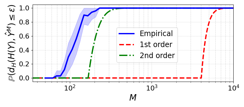
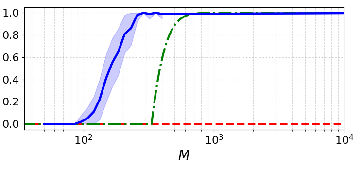
We numerically evaluate the tightness of the bounds from Corollary 5.2. As in [LJBP22], let $\mathcal{X}=B(0,1)\subset\mathbb{R}^{2}$ and $f:x\mapsto(Lx^{1},x^{2})$ for $L>0$, so that $\mathcal{Y}=f(\mathcal{X})$ is an ellipsoid. We sample $M$ inputs $x_{i}$ from a uniform distribution $\mathbb{P}_{\mathcal{X}}$ over $\partial\mathcal{X}$, which satisfies Assumption 5.1. $\mathcal{X}$ is $1$-smooth, $f$ is a diffeomorphism (and thus a submersion), and $(f,\textrm{d}f)$ are $(\max(1,L),0)$-Lipschitz, so the assumptions of Corollary 5.2 hold. For a desired accuracy $\epsilon=10^{-2}$, using the first- and second-order bounds from Corollary 5.2, we determine $\beta_{M,\delta}^{\partial\mathcal{X}}=\eqref{eq:delta:sampling_density:boundary}$ to achieve a Hausdorff distance error $d_{H}(\textrm{H}(\mathcal{Y}),\hat{\mathcal{Y}}^{M})\leq\epsilon$ with probability at least $1-\beta_{M,\delta}^{\partial\mathcal{X}}$ for different sample sizes $M$.

We compare the bounds $1-\beta_{M,\delta}^{\partial\mathcal{X}}$ given by Corollary 5.2 with the empirical average number of trials that achieve $\epsilon$-accuracy (we use $100$ independent trials for each value of $M$). Results for different sample sizes $M$ are shown in Figure 8. We observe that the second-order error bounds are quite sharp in the case $L=1$ and are an order of magnitude tighter than the first-order error bounds. Bounds become more conservative for larger values of $L$.

5.2   Reachability analysis of uncertain dynamical systems

Next, we consider the problem of estimating the convex hull of all reachable states of a dynamical system at a given time in the future. Such reachable sets play an important role in many applications ranging from robust predictive control [SKA18, SZBZ22] to neural network verification [EHCH21]. Empirically, sampling-based approaches can provide accurate reconstructions of convex hulls of reachable sets from relatively few inputs [LP20, LJBP22]. However, previous error bounds [LJBP22] rely on naive Lipschitz-covering arguments and do not match empirical results, see Figure 8.

Let $\mathcal{X}_{0}\subset\mathbb{R}^{n}$, $\Theta\subset\mathbb{R}^{p}$, and $U\subset\mathbb{R}^{m}$ be non-empty compact sets of initial conditions, parameters, and admissible control inputs. Let $f:\mathbb{R}^{n}\times\mathbb{R}^{p}\times\mathbb{R}^{m}\times\mathbb{R}\to\mathbb{R}^{n}$ be a continuous map that is Lipschitz in its first argument, i.e., for some $L\geq 0$, $\|f(x_{1},\theta,u,t)-f(x_{2},\theta,u,t)\|\leq L\|x_{1}-x_{2}\|$ for all $x_{1},x_{2}\in\mathbb{R}^{n},\theta\in\Theta,u\in U,t\in\mathbb{R}$. Given $T>0$, the ordinary differential equation (ODE)

$$\dot{x}(t)=f(x(t),\theta,u(t),t),\quad t\in[0,T],\quad x(0)=x^{0}$$ (8)

has a unique solution $x_{u}^{x^{0},\theta}\in C([0,T],\mathbb{R}^{n})$ for any $u\in L^{2}([0,T],U)$. For any $t\in[0,T]$, the map $x^{0}\mapsto x_{u}^{x^{0},\theta}(t)$ is a diffeomorphism, so $(x^{0},\theta)\mapsto x_{u}^{x^{0},\theta}(t)$ is a submersion. Define the reachable set

$$\mathcal{Y}_{u}(t) =\left\{x_{u}^{x^{0},\theta}(t)=x^{0}+\int_{0}^{t}f\big{(}x_{u}^{x^{0},\theta}(s),\theta,u(s),s\big{)}\textrm{d}s:(x^{0},\theta)\in\mathcal{X}\right\}.$$

where $\mathcal{X}\subset\mathbb{R}^{n+p}$ is any approximation with smooth boundary of $\mathcal{X}_{0}\times\Theta$. Theorem 1.1 implies that $\textrm{H}(\mathcal{Y}_{u}(t))$ can be accurately estimated using inputs in $\partial\mathcal{X}$.

Corollary 5.3.

Let $r,\delta>0$, $Z_{\delta}=\{(x_{i}^{0},\theta_{i})\}_{i=1}^{M}\subset\partial\mathcal{X}$ be a $\delta$-cover of $\partial\mathcal{X}$, and assume that $\mathcal{X}$ is non-empty, compact, path-connected, and $r$-smooth. Let $u\in L^{2}([0,T],U)$, $t\in\mathbb{R}$, $\hat{\mathcal{Y}}_{u}^{M}(t)=\textrm{H}\big{(}\{x_{u}^{x_{i}^{0},\theta_{i}}(t)\}_{i=1}^{M}\big{)}$, and $(\bar{L}_{u},\bar{H}_{u})$ the Lipschitz constants of $(x^{0},\theta)\mapsto(x_{u}^{x^{0},\theta}(t),\textrm{d}x_{u}^{x^{0},\theta}(t))$. Then, $d_{H}\big{(}\textrm{H}(\mathcal{Y}_{u}(t)),\hat{\mathcal{Y}}_{u}^{M}(t)\big{)}\leq\frac{1}{2}\big{(}\frac{\bar{L}_{u}}{r}+\bar{H}_{u}\big{)}\delta^{2}$.

The smoothness constants of the map $(x^{0},\theta)\mapsto x_{u}^{x^{0},\theta}(t)$ depend on properties of $f$ in (8). For example, tight bounds can be derived if the system in (8) is contracting [WS20]. Such analysis is problem-specific and left for future work.

5.3   Robust optimization

Next, we apply our analysis to study the feasibility of approximations to non-convex robust programs. Let $\mathcal{X}\subset\mathbb{R}^{m}$ be a compact set, $\mathcal{C}\subseteq\mathbb{R}^{n}$ be a closed convex set, $\ell:\mathbb{R}^{p}\to\mathbb{R}$ and $f:\mathbb{R}^{m}\times\mathbb{R}^{p}\to\mathbb{R}^{n}$ be two continuous functions, and define the robust optimization problem

$$\mathbf{P}:\ \inf_{u\in\mathbb{R}^{p}}\ell(u)\ \ \text{s.t.}\ \ f(x,u)\in\mathcal{C}\ \text{for all }x\in\mathcal{X}.$$

If $\mathcal{X}$ is infinite (e.g., if $\mathcal{X}=B(0,r)$ is a ball of parameters), then P has an infinite number of constraints that can be approximated as follows. Given $M$ sampled inputs $x_{i}\in\mathcal{X}$ and a padding $\epsilon>0$, define the relaxation

$$\hat{\mathbf{P}}_{\epsilon}^{M}:\ \inf_{u\in\mathbb{R}^{p}}\ell(u)\ \ \text{s.t.}\ \ f(x_{i},u)+B(0,\epsilon)\subseteq\mathcal{C}\ \text{for all }i=1,\dots,M.$$

For instance, if $\mathcal{C}$ is an intersection of hyperplanes $\mathcal{C}_{j}=\{y\in\mathbb{R}^{n}:n_{j}^{\top}(y-c_{j})\leq 0,c_{j}\in\mathbb{R}^{n},\|n_{j}\|=1\}$, then the constraints in $\hat{\mathbf{P}}_{\epsilon}^{M}$ are equivalent to $n_{j}^{\top}(f(x_{i},u)-c_{j})+\epsilon\leq 0$ for all $i=1,\dots,M$ and $j$. In this case, $\hat{\mathbf{P}}_{\epsilon}^{M}$ is a tractable finite-dimensional relaxation of $\mathbf{P}$.

Thanks to Theorem 1.1, solving $\hat{\mathbf{P}}_{\epsilon}^{M}$ yields feasible solutions of $\mathbf{P}$ given sufficiently many sampled inputs $x_{i}$ on the boundary $\partial\mathcal{X}$. If $f$ is a submersion, a small sample size $M$ suffices.

Corollary 5.4.

Let $r,\delta>0$, $\mathcal{X}\subset\mathbb{R}^{m}$ be a non-empty path-connected compact $r$-smooth set, $\{x_{i}\}_{i=1}^{M}\subset\partial\mathcal{X}$ be a $\delta$-cover of $\partial\mathcal{X}$, $f$ be such that $f_{u}=f(\cdot,u)$ is a $C^{1}$ submersion and $(f_{u},\textrm{d}f_{u})$ are $(\bar{L},\bar{H})$-Lipschitz for all $u\in\mathbb{R}^{p}$, and $\epsilon\geq\frac{1}{2}\big{(}\frac{\bar{L}_{u}}{r}+\bar{H}_{u}\big{)}\delta^{2}$. Then, any solution of $\hat{\mathbf{P}}_{\epsilon}^{M}$ is feasible for $\mathbf{P}$.

Corollary 5.4 justifies solving the relaxed problem $\hat{\mathbf{P}}_{\epsilon}^{M}$ to obtain feasible solutions of $\mathbf{P}$. The analysis of the suboptimality gap is left for future work. We provide an application of this result next.

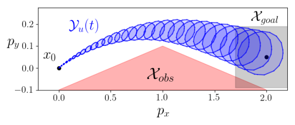
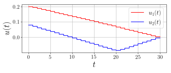
5.4   Numerical example: planning under bounded uncertainty

We consider the following optimal control problem (OCP) under bounded uncertainty:

$$\textbf{OCP}:\quad\inf_{u\in\mathcal{U}}\qquad \int_{0}^{T}\|u(t)\|^{2}\textrm{d}t$$ (min. fuel consumption)

s.t. $$\dot{p}(t)=v(t),\ \dot{v}(t)=\frac{1}{m}(u(t)+F),\ \ t\in[0,T],$$ (dynamics)

$$Hp(t)\leq h,\hskip 110.96574ptt\in[0,T],\ \$$ (obstacle avoidance)

$$Gp(T)\leq g,\quad(p(0),v(0))=0,$$ (initial & final conditions)

$$(m,F)\in\mathcal{X},$$ (uncertain parameters)

where $(p(t),v(t))\in\mathbb{R}^{4}$ denote the position and velocity of the system, $u(t)\in\mathbb{R}^{2}$ is the control input, $(m,F)\in\mathcal{X}\subset\mathbb{R}^{3}$ correspond to the uncertain mass of the system and constant disturbance, $H,h,G,g$ define the obstacle-free statespace and goal region, $T$ is the planning horizon, and we optimize over control trajectories $u\in\mathcal{U}\subset L^{2}([0,T],\mathbb{R}^{2})$ that are piecewise-constant on a partition of $[0,T]$, as is common in applications such as model predictive control [SKA18, SZBZ22]. The dynamics may correspond to a spacecraft system [LJBP22] carrying an uncertain payload subject to constant disturbances.

Although the dynamics are linear in the control input, the dynamics are nonlinear in the uncertain parameters $(m,F)$. The resulting uncertainty over the state trajectory is correlated over time, which makes solving OCP challenging. This contrasts with problems with additive independent disturbances for which a wide range of numerical resolution schemes exist. We refer to [LJBP22] for a discussion of existing methods for reachability analysis of such systems.

We study the problem in detail in Section C.4. We consider the uncertainty set $(m,F)\in[30,34]\times B(0,5\cdot 10^{-3})$ and show how to outer-bound these inputs with an $r$-smooth compact set $\mathcal{X}$. Then, we show that the map $(m,F)\mapsto p_{u}^{m,F}(t)$ is a submersion and study its smoothness. The assumptions of Corollaries 5.3 and 5.4 hold, so we evaluate the bound on the Hausdorff distance $d_{H}\big{(}\textrm{H}(\mathcal{Y}_{u}(t)),\hat{\mathcal{Y}}_{u}^{M}(t)\big{)}\leq\epsilon=0.025$ for $M=100$ inputs $(m_{i},F_{i})$, which is sufficiently accurate. We discretize OCP in time and express the finite-dimensional relaxation where constraints are only evaluated at the $M$ inputs $(m_{i},F_{i})$ as described in Section 5.3. We solve the resulting convex program in approximately $200\,\textrm{ms}$ (measured on a laptop with a 1.10GHz Intel Core i7-10710U CPU) using OSQP [SBG⁺20] and present results in Figure 9. As guaranteed by Corollary 5.4, the obtained trajectory is collision-free and reaches the goal region for all uncertain parameters $(m,F)$. We note that $M=3300$ inputs would be necessary to provably achieve the same level of precision with a naive bound that only leverages the Lipschitzness of $p_{u}^{m,F}(t)$ (see Lemma 4.2), and solving the resulting approximation of OCP would take over $25\,\textrm{s}$.

Figure 9: Solution of the finite-dimensional approximation of OCP.

6   Conclusion

We derived new error bounds for the estimation of the convex hull of the image $f(\mathcal{X})$ of a set $\mathcal{X}$ with smooth boundary. Our results show that accurate reconstructions are possible using a few sampled inputs $x_{i}$ on the boundary of $\mathcal{X}$. We provided numerical experiments demonstrating the tightness of our bounds in practical applications.

Of immediate interest for future research is deriving error bounds for non-convex approximations of the output set $f(\mathcal{X})$ (e.g., for tangential Delaunay complexes [BG13, AL18]) from assumptions on $f$ and $\mathcal{X}$. Extending the results to the presence of noise corrupting the sample [AL18, AK22] would allow reconstructing $f(\mathcal{X})$ from sampled inputs that are not exactly on the boundary of $\mathcal{X}$. Potentially, this would also allow accurate reconstructions using approximate models of $f$. Applications of our results include the design of more efficient control algorithms that explicitly account for uncertainty.

Appendix A Proofs for Section 2.2

Proof of Lemma 2.3.

Our proof follows the proof of [CFPL12, Proposition 1].

We denote by $\pi(x)\in\mathcal{X}$ the projection of any $x\in\mathbb{R}^{n}$ onto $\mathcal{X}$, which is unique if $d_{\mathcal{X}}(x)<r$ since $\textrm{reach}(\mathcal{X})\geq r$. To show that $\mathcal{X}$ is $r$-convex, it suffices to show that for all $x\in\mathcal{X}^{\mathsf{c}}$, there exists $y\in\mathring{B}(x,r)$ such that $\mathring{B}(y,r)\cap\mathcal{X}=\emptyset$.

Let $x\in\mathcal{X}^{\mathsf{c}}$. If $d_{\mathcal{X}}(x)\geq r$, then $\mathring{B}(x,r)\cap\mathcal{X}=\emptyset$. If $d_{\mathcal{X}}(x)<r$, let $\pi(x)$ be the unique point in $\mathcal{X}$ such that $d_{\mathcal{X}}(x)=\|x-\pi(x)\|$. Then, $n(x)=\frac{x-\pi(x)}{\|x-\pi(x)\|}\in\text{Nor}(\mathcal{X},\pi(x))$, where $\text{Nor}(\mathcal{X},\pi(x))$ denotes the set of all normal vectors of $\mathcal{X}$ at $\pi(x)$ (see the definition in [Fed59] which does not assume that $\partial\mathcal{X}$ is a submanifold).

Define $y_{\lambda}=\pi(x)+\lambda n(x)$ for $0<\lambda\leq r$. Note that $y_{\lambda}\in\mathring{B}(x,r)$; in particular, $y_{r}\in\mathring{B}(x,r)$.

Let $0<\lambda<r$. Since $\textrm{reach}(\mathcal{X})\geq r>\lambda$, [Fed59, Theorem 4.8] gives that $n(x)=\frac{v}{\lambda}$ for some $v\in\mathbb{R}^{n}$ with $\|v\|=\lambda$ and that $\pi(y_{\lambda})=\pi(\pi(x)+v)=\pi(x)$. Then, $\mathring{B}(y_{\lambda},\lambda)\cap\mathcal{X}=\emptyset$ (the last statement follows from $\pi(y_{\lambda})=\pi(x)$: by contradiction, assume that there exists $z\in\mathcal{X}$ with $\|y_{\lambda}-z\|<\lambda$. Then, $\|y_{\lambda}-\pi(y_{\lambda})\|=\|y_{\lambda}-\pi(x)\|<\lambda$, which contradicts $\|y_{\lambda}-\pi(x)\|=\|\lambda n(x)\|=\lambda$.).

Finally, $\mathring{B}(y_{\lambda},\lambda)\cap\mathcal{X}=\emptyset$ for $0<\lambda<r$ implies that $\mathring{B}(y_{r},r)\cap\mathcal{X}=\emptyset$. Indeed, if $z\in\mathring{B}(y_{r},r)$, then $z\in\mathring{B}(y_{\lambda},\lambda)$ for some $0<\lambda<r$ (indeed, assume that $\|y_{r}-z\|=r-\epsilon$ with $0<\epsilon<r$. Then, $\|y_{\lambda}-z\|\leq\|y_{\lambda}-y_{r}\|+\|y_{r}-z\|=r-\lambda+r-\epsilon<\lambda$ for $\lambda=r-\frac{\epsilon}{4}$). The conclusion follows. ∎

Proof of Lemma 2.4.

Let $x\in\partial\mathcal{X}$ and $0<\lambda\leq r$ (the result is trivial if $\lambda=0$). A ball of radius $R$ rolls freely in $\mathcal{X}$; let $a\in\mathcal{X}$ be such that $x\in B(a,R)\subseteq\mathcal{X}$. Denoting by $n(x)=\frac{x-a}{\|x-a\|}$ the outward-pointing unit-norm normal of $\partial B(a,R)$ at $x$, we define $a_{\lambda}=x-\lambda n(x)$. Then, $x\in B(a_{\lambda},\lambda)$ since $\|x-a_{\lambda}\|=\lambda$, and $n(x)$ is also the outward-pointing unit-norm normal of $\partial B(a_{\lambda},\lambda)$. Since $\frac{1}{\lambda}\geq\frac{1}{R}$, by [Rau74], $B(a_{\lambda},\lambda)\subseteq B(a,R)\subseteq\mathcal{X}$. We conclude that a ball of radius $0\leq\lambda\leq R$ rolls freely in $\mathcal{X}$. The proof that a ball of radius $\lambda$ rolls freely in $\overline{\mathcal{X}^{\mathsf{c}}}$ is identical. ∎

Proof of Lemma 2.5.

The result follows from the supporting hyperplane theorem, see [Sch14, Theorem 1.3.2]. ∎

Appendix B Proofs for Section 4.2.2 (bound on $d_{T_{y}\partial\textrm{H}(\mathcal{Y})}$)

B.1   Modifications for Lemma 4.5 if $f$ is only $C^{1}$

In this section, we sketch the minor modifications to the proof of Lemma 4.5 in Section 4 to handle the case where $f$ is only $C^{1}$ (if $f$ is only $C^{1}$, using $\textrm{d}^{2}f$ is not rigorous). The result can be justified using Taylor’s Theorem [Fol90], which states that any $C^{1}$ scalar function $g:\mathbb{R}\to\mathbb{R}$ satisfies

$$g(b)=g(a)+g^{\prime}(a)(b-a)+(b-a)\int_{0}^{1}\left(g^{\prime}(a+u(b-a))-g^{\prime}(a)\right)\textrm{d}u.$$

For simplicity, consider the scalar case where $f:\mathbb{R}\to\mathbb{R}$ is $C^{1}$ and $\gamma:\mathbb{R}\to\mathbb{R}$ is $C^{2}$. Then,

$$f(\gamma(t))-f(\gamma(0))-t(f\circ\gamma)^{\prime}(0) =t\int_{0}^{1}\left((f\circ\gamma)^{\prime}(ut)-(f\circ\gamma)^{\prime}(0)\right)\textrm{d}u$$

$$=t\int_{0}^{1}\left(\textrm{d}f_{\gamma(ut)}(\gamma^{\prime}(ut))-\textrm{d}f_{\gamma(0)}(\gamma^{\prime}(0))\right)\textrm{d}u$$

$$=t\int_{0}^{1}\left(\textrm{d}f_{\gamma(ut)}(\gamma^{\prime}(0))-\textrm{d}f_{\gamma(0)}(\gamma^{\prime}(0))\right)\textrm{d}u.$$

using the fact that $\gamma^{\prime\prime}(s)=0$ so that $\gamma^{\prime}(ut)=\gamma^{\prime}(0)$.

Assuming that $\textrm{d}f$ is $\bar{H}$-Lipschitz, $\|\textrm{d}f_{\gamma(ut)}(\gamma^{\prime}(0))-\textrm{d}f_{\gamma(0)}(\gamma^{\prime}(0))\|\leq\bar{H}\|\gamma(ut)-\gamma(0)\|\|\gamma^{\prime}(0)\|$ and

$$\left\|f(\gamma(t))-f(\gamma(0))-t(f\circ\gamma)^{\prime}(0)\right\| =\left\|t\int_{0}^{1}\left(\textrm{d}f_{\gamma(ut)}(\gamma^{\prime}(0))-\textrm{d}f_{\gamma(0)}(\gamma^{\prime}(0))\right)\textrm{d}u\right\|$$

$$\leq t\int_{0}^{1}\bar{H}\|\gamma(ut)-\gamma(0)\|\|\gamma^{\prime}(0)\|\textrm{d}u$$

$$=\bar{H}\frac{t^{2}}{2}$$

using $\gamma(ut)-\gamma(0)=t\gamma^{\prime}(0)$ and $\|\gamma^{\prime}(0)\|=1$. Thus, with minor modifications, the proof of Lemma 4.5 only requires assuming that $f\in C^{1}$ as claimed.

B.2   Proof of Lemma 4.6 (curve intersecting a ball)

We first define a suitable chart to prove Lemma 4.6.

Let $B\subset\mathbb{R}^{n}$ be an $n$-dimensional closed ball of radius $r>0$ in $\mathbb{R}^{n}$, whose boundary $\partial B\subset\mathbb{R}^{n}$ is an $(n-1)$-dimensional submanifold of $\mathbb{R}^{n}$. We denote the normal bundle of $\partial B$ by $N(\partial B)$ and the outward-pointing unit-norm normal of $\partial B$ by $n^{\partial B}$, which defines a smooth frame for $N(\partial B)$. The restriction of the exponential map in $\mathbb{R}^{n}$ to the normal bundle of $\partial B$ is defined as

$$E:N(\partial B)\to\mathbb{R}^{n}:(x,v)\mapsto x+v.$$

Let $U\subset\mathbb{R}^{n}$ be a uniform tubular neighborhood of $\partial B$ in $\mathbb{R}^{n}$, see [Lee18, Theorem 5.25]. Then, there is an open set

$$V_{\delta}=\Big{\{}(x,sn^{\partial B}(x))\in N(\partial B):s\in(-\delta,\delta)\Big{\}}$$

for some $\delta>0$ such that the map

$$E:V_{\delta}\to U,\ \big{(}x,sn^{\partial B}(x)\big{)}\mapsto x+sn^{\partial B}(x)$$

is a diffeomorphism. Next, we define the smooth map

$$\psi:\partial B\times(-\delta,\delta)\to V_{\delta},\ (x,s)\mapsto\big{(}x,sn^{\partial B}(x)\big{)}$$

which is a diffeomorphism since its differential is an isomorphism. Therefore, the smooth map

$$(E\circ\psi):\partial B\times(-\delta,\delta)\to U$$

is a diffeomorphism. Finally, we define the following chart of $\mathbb{R}^{n}$

$$\varphi=(E\circ\psi)^{-1}:U\to\partial B\times(-\delta,\delta).$$

which satisfies $\varphi(y)=(x,s)\in\partial B\times(-\delta,\delta)$ for any $y=x+sn^{\partial B}(x)\in U$. Since $n^{\partial B}$ is outward-pointing, the last component of $\varphi$ satisfies

• $\varphi^{n}(y)>0\iff y\in B^{\mathsf{c}}$,

• $\varphi^{n}(y)=0\iff y\in\partial B$,

• $\varphi^{n}(y)<0\iff y\in\textrm{Int}(B)$.

Proof of Lemma 4.6.

In the following, we use the coordinates defined previously.

Define $f(t)=\varphi^{n}(\gamma(t))$. Since $\gamma(t)\in\textrm{Int}(B)$ if and only if $f(t)=\varphi^{n}(\gamma(t))<0$, it suffices to prove that $f(t)<0$ for some $t\in(-\epsilon,\epsilon)$. Since $f(t)$ is smooth and $f(0)=\varphi^{n}(\gamma(0))=\varphi^{n}(p)=0$, it suffices to prove that $f^{\prime}(0)<0$ or $f^{\prime}(0)>0$.

$f^{\prime}(0)=\frac{\textrm{d}}{\textrm{d}t}\left(\varphi^{n}(\gamma(t))\right)\big{|}_{t=0}=\left(\textrm{d}\varphi^{n}_{\gamma(t)}(\gamma^{\prime}(t))\right)\Big{|}_{t=0}=\textrm{d}\varphi^{n}_{p}(v)$. Since $\textrm{d}\varphi^{n}_{p}(v)=0$ if and only if $v\in T_{p}\partial B$, but $v\notin T_{p}\partial B$ by assumption, we obtain that $f^{\prime}(0)\neq 0$. This concludes the proof. ∎

B.3   Proof of Lemma 4.7 ($\textrm{d}f_{x}(T_{x}\partial\mathcal{X})=T_{y}\partial\textrm{H}(\mathcal{Y})$)

B.3.1 Problem definition and setup

• Let $r>0$ and $\mathcal{X}\subset\mathbb{R}^{m}$ be a non-empty path-connected $r$-smooth compact set.

  • By Theorem 2.1, $\partial\mathcal{X}\subset\mathbb{R}^{m}$ is a $(m-1)$-dimensional submanifold with unique normal $n^{\partial\mathcal{X}}(x)$.

  • By Theorem 2.1, an $m$-dimensional ball of radius $r>0$ rolls freely inside $\mathcal{X}$ and $\overline{\mathcal{X}^{\mathsf{c}}}$.

• Let $f:\mathbb{R}^{m}\to\mathbb{R}^{n}$ be a smooth submersion.

• Let $\mathcal{Y}=f(\mathcal{X})$.

• Let $y\in\partial\mathcal{Y}\cap\partial\textrm{H}(\mathcal{Y})$.

• Let $x\in\partial\mathcal{X}$ be such that $y=f(x)$ (this input $x$ exists since $\partial\mathcal{Y}\subseteq f(\partial\mathcal{X})$ by Lemmas 3.5 and 3.6 since $f$ is a submersion).

  • By the rank theorem, there exist two charts $((U,\varphi),(V,\psi))$ centered at $x$ such that $\psi\circ f\circ\varphi^{-1}$ is a coordinate projection:

    $$\psi\circ f\circ\varphi^{-1}:\varphi(U\cap f^{-1}(V))\to\psi(V),\ (\hat{x}_{1},\dots,\hat{x}_{n},\hat{x}_{n+1},\dots\hat{x}_{m})\mapsto(\hat{x}_{1},\dots,\hat{x}_{n}).$$

    In other words, $(\psi\circ f\circ\varphi^{-1})|_{\varphi(U\cap f^{-1}(V))}(\cdot)=\pi(\cdot)$ is the projection from $\mathbb{R}^{m}$ to $\mathbb{R}^{n}$.

• Let $P=\{\hat{x}\in\mathbb{R}^{m}:\hat{x}_{n+1}=\dots=\hat{x}_{m}=0\}$ and $Q=\{\hat{x}\in\mathbb{R}^{m}:\hat{x}_{1}=\dots=\hat{x}_{n}=0\}$.

• Let $S=\varphi^{-1}\left(P\cap\varphi(U)\right)$.

• Let $B\subseteq\mathcal{X}$ be a tangent ball at $x$ inside $\mathcal{X}$ of radius $\min(r,\textrm{reach}(S))>0$ with $T_{x}\partial B=T_{x}\partial\mathcal{X}$. This ball exists by Theorem 2.1, and $\textrm{reach}(S)>0$ since $S$ is a submanifold.

• Let $Z=S\cap\partial B$.

We claim that $\textrm{d}f_{x}(T_{x}\partial\mathcal{X})=T_{y}\partial\textrm{H}(\mathcal{Y})$.

Figure 10: Definitions for the proof of Lemma 4.7.

B.3.2 Properties

First, $f^{-1}(y)\subset\mathbb{R}^{m}$ is a $(m-n)$-dimensional submanifold and $T_{x}f^{-1}(y)=\textrm{Ker}(\textrm{d}f_{x})$ since $f$ is a submersion (see Theorem 5.12 and Proposition 5.38 in [Lee12]). The following properties are used in the proof of Lemma 4.7.

Property B.1.

$\textrm{Ker}(\textrm{d}f_{x})=\textrm{d}(\varphi^{-1})_{\varphi(x)}\left(T_{\varphi(x)}Q\right)$.

Property B.2.

$T_{x}\mathbb{R}^{m}=T_{x}S+\textrm{Ker}(\textrm{d}f_{x})$.

Property B.3.

$T_{x}f^{-1}(y)\subseteq T_{x}\partial\mathcal{X}$.

Property B.4.

$Z$ is a submanifold of dimension $(n-1)$.

Property B.5.

$T_{x}\partial\mathcal{X}=T_{x}Z+T_{x}f^{-1}(y)$.

Property B.6.

$T_{y}\partial\textrm{H}(\mathcal{Y})=T_{y}f(Z)$.

B.3.3 Proofs of Properties B.1-B.6

Proof of Property B.1: $\textrm{Ker}(\textrm{d}f_{x})=\textrm{d}(\varphi^{-1})_{\varphi(x)}\left(T_{\varphi(x)}Q\right)$.

First, we show that $\textrm{d}(\varphi^{-1})_{\varphi(x)}(T_{\varphi(x)}Q)\subseteq\textrm{Ker}(\textrm{d}f_{x})$. Let $v\in\textrm{d}(\varphi^{-1})_{\varphi(x)}(T_{\varphi(x)}Q)$ and $w=\textrm{d}\varphi_{x}(v)\in T_{\varphi(x)}Q$. Then,

$$\textrm{d}f_{x}(v) =\textrm{d}(\psi^{-1}\circ\pi\circ\varphi)_{x}(\textrm{d}(\varphi^{-1})_{\varphi(x)}(w))=\textrm{d}(\psi^{-1})_{\pi(\varphi(x))}(\textrm{d}\pi_{\varphi(x)}(w))=\textrm{d}(\psi^{-1})_{\pi(\varphi(x))}(0)=0$$

since $\textrm{d}\pi_{\varphi(x)}(T_{\varphi(x)}Q)=0$ by definition of $Q$. Thus, $v\in\textrm{Ker}(\textrm{d}f_{x})$.

Second, $\dim(\textrm{d}(\varphi^{-1})_{\varphi(x)}(T_{\varphi(x)}Q))=\dim(T_{\varphi(x)}Q)=m-n$, since $\varphi^{-1}$ is a diffeomorphism.

Thus, $\dim(\textrm{d}(\varphi^{-1})_{\varphi(x)}(T_{\varphi(x)}Q))=\dim(\textrm{Ker}(\textrm{d}f_{x}))$ and $\textrm{d}(\varphi^{-1})_{\varphi(x)}(T_{\varphi(x)}Q)\subseteq\textrm{Ker}(\textrm{d}f_{x})$.

The conclusion follows. ∎

Proof of Property B.2: $T_{x}\mathbb{R}^{m}=T_{x}S+\textrm{Ker}(\textrm{d}f_{x})$.

Indeed, since $\varphi^{-1}$ is a diffeomorphism,

$$T_{x}\mathbb{R}^{m} =\textrm{d}(\varphi^{-1})_{\varphi(x)}(T_{\varphi(x)}\mathbb{R}^{m})$$

$$=\textrm{d}(\varphi^{-1})_{\varphi(x)}(T_{\varphi(x)}P+T_{\varphi(x)}Q)$$

$$=T_{x}S+\textrm{d}(\varphi^{-1})_{\varphi(x)}(T_{\varphi(x)}Q))$$

$$=T_{x}S+\textrm{Ker}(\textrm{d}f_{x}).$$ (Property B.1)

∎

We observe that up to Property B.2, we did not use the fact that $y\in\partial\mathcal{Y}$.

Proof of Property B.3: $T_{x}f^{-1}(y)\subseteq T_{x}\partial\mathcal{X}$.

By contradiction, assume that $T_{x}f^{-1}(y)\nsubseteq T_{x}\partial\mathcal{X}$. Then, there is some $v\in T_{x}f^{-1}(y)$ but $v\notin T_{x}\partial\mathcal{X}=T_{x}\partial B$.

Let $I=(-\epsilon,\epsilon)$ and $\gamma:I\to f^{-1}(y)$ be a curve with $\gamma(0)=x$ and $\gamma^{\prime}(0)=v$. By definition, this curve satisfies $f(\gamma(t))=y\in\partial\mathcal{Y}$ for all $t\in I$. However, by Lemma 4.6, there exists $s\in I$ such that $\gamma(s)\in\textrm{Int}(B)$, since $\gamma^{\prime}(0)=v\notin T_{x}\partial B$. Thus, $y=f(\gamma(s))\in f(\textrm{Int}(B))\subseteq f(\textrm{Int}(\mathcal{X}))\subseteq\textrm{Int}(f(\mathcal{X}))=\textrm{Int}(\mathcal{Y})$, since $f$ is an open map (since it is a submersion, see Lemma 3.5). Thus, $y\in\textrm{Int}(\mathcal{Y})$, which is a contradiction since $y\in\partial\mathcal{Y}$. ∎

Proof of Property B.4: $Z$ is a submanifold of dimension $(n-1)$.

We proceed in three steps.

• Step 1: The open ball $\mathring{B}$ intersects $S$. First, we show that $T_{x}\mathbb{R}^{m}=T_{x}S+T_{x}\partial B$. Indeed,

  $$T_{x}\mathbb{R}^{m} =T_{x}S+\textrm{Ker}(\textrm{d}f_{x})$$ (Property B.2)

  $$=T_{x}S+T_{x}f^{-1}(y)$$

  $$\subseteq T_{x}S+T_{x}\partial\mathcal{X}$$ (Property B.3)

  $$=T_{x}S+T_{x}\partial B.$$

  Thus, $T_{x}\mathbb{R}^{m}=T_{x}S+T_{x}\partial B$. Since $\dim(T_{x}\partial B)=m-1$, this implies that there exists $v\in T_{x}S$ with $v\notin T_{x}\partial B$.

  Let $\gamma:(-\epsilon,\epsilon)\to S$ be any smooth curve with $\gamma(0)=x$ and $\gamma^{\prime}(0)=v$. By Lemma 4.6, $\gamma(t)\in\textrm{Int}(B)$ for some $t\in(-\epsilon,\epsilon)$. Thus, $\gamma(t)\in S\cap\textrm{Int}(B)$. We obtain that the open ball $\mathring{B}$ intersects $S$.

• Step 2: $T_{\tilde{x}}\mathbb{R}^{m}=T_{\tilde{x}}S+T_{\tilde{x}}\partial B$ for all $\tilde{x}\in S\cap\partial B$. By contradiction, assume that $T_{\tilde{x}}\mathbb{R}^{m}\neq T_{\tilde{x}}S+T_{\tilde{x}}\partial B$ for some $\tilde{x}\in S\cap\partial B$. Since $\dim(T_{\tilde{x}}\partial B)=m-1$, this implies that $T_{\tilde{x}}S\subseteq T_{\tilde{x}}\partial B$. Thus, the ball $B$ is tangent to $S$ at $\tilde{x}$.

  Since $B$ has a radius smaller than $\textrm{reach}(S)$ and is tangent to $S$ at $\tilde{x}$ by the above, the open ball $\mathring{B}$ does not intersect $S$ [BLW19, Corollary 2]. This contradicts Step 1.

• Step 3: Conclude by transversality. By Step 2, $\textrm{Span}(T_{\tilde{x}}S,T_{\tilde{x}}\partial B)=T_{\tilde{x}}\mathbb{R}^{m}$ for all $\tilde{x}\in S\cap\partial B$. Thus, by transversality [Lee12, Theorem 6.30], $Z=S\cap\partial B$ is a submanifold of dimension $m-(\textrm{codim}(S)+\textrm{codim}(\partial B))=m-(m-n+1)=n-1$. The conclusion follows.

∎

Proof of Property B.5: $T_{x}\partial\mathcal{X}=T_{x}Z+T_{x}f^{-1}(y)$.

$$\dim\left(\textrm{Span}(T_{x}Z,\,T_{x}f^{-1}(y))\right) =\dim\left(\textrm{Span}(\textrm{d}\varphi_{x}(T_{x}Z),\,\textrm{d}\varphi_{x}(T_{x}f^{-1}(y)))\right) \varphi$$ ( is a diffeomorphism)

$$=\dim\left(\textrm{Span}(\textrm{d}\varphi_{x}(T_{x}Z),\,T_{\varphi(x)}Q)\right)$$ (Property B.1)

$$=\dim(\textrm{d}\varphi_{x}(T_{x}Z))+\dim(T_{\varphi(x)}Q) \textrm{d}\varphi_{x}(T_{x}Z)\subset T_{\varphi(x)}P\text{ and }T_{\varphi(x)}P\perp T_{\varphi(x)}Q$$ ()

$$=(n-1)+(m-n)=m-1.$$

Thus, $\dim\left(\textrm{Span}(T_{x}Z,\,T_{x}f^{-1}(y))\right)=\dim(T_{x}\partial\mathcal{X})$. Since $T_{x}Z\subseteq T_{x}\partial\mathcal{X}$ (since $Z\subseteq\partial\mathcal{X}$) and $T_{x}f^{-1}(y)\subseteq T_{x}\partial\mathcal{X}$ (Property B.3), we obtain that $T_{x}\partial\mathcal{X}=T_{x}Z+T_{x}f^{-1}(y)$. ∎

We recall that $\partial\textrm{H}(\mathcal{Y})$ is a submanifold of dimension $(n-1)$ by Corollary 3.8. Also, $f(Z)\subset\mathbb{R}^{n}$ is a submanifold, since $Z\subset S$ is a submanifold (Property B.4) and $f|_{S}$ is a diffeomorphism.

Proof of Property B.6: $T_{y}\partial\textrm{H}(\mathcal{Y})=T_{y}f(Z)$.

By contradiction, assume that $T_{y}\partial\textrm{H}(\mathcal{Y})\neq T_{y}f(Z)$. Then, there exists $v\in T_{y}f(Z)$ such that $v\notin T_{y}\partial\textrm{H}(\mathcal{Y})$, since $\dim(\partial\textrm{H}(\mathcal{Y}))=n-1=\dim(T_{y}f(Z))$ (note that $f|_{S}$ is a diffeomorphism and $Z\subset S$, so $\dim(T_{y}f(Z))=\dim(T_{x}Z)=n-1$).

Let $\tilde{B}\subset\overline{\textrm{H}(\mathcal{Y})^{\mathsf{c}}}$ be a ball outside $\textrm{H}(\mathcal{Y})$ that is tangent to $\textrm{H}(\mathcal{Y})$ at $y$ (such that $T_{y}\partial\tilde{B}=T_{y}\partial\textrm{H}(\mathcal{Y})$). Such a ball exists since $\textrm{H}(\mathcal{Y})$ is convex.

Let $\gamma:(-\epsilon,\epsilon)\to f(Z)$ be a smooth curve with $\gamma(0)=y$ and $\gamma^{\prime}(0)=v$. Since $v\notin T_{y}\partial\tilde{B}=T_{y}\partial\textrm{H}(\mathcal{Y})$, by Lemma 4.6, $\gamma(s)\in\textrm{Int}(\tilde{B})\subset\textrm{H}(\mathcal{Y})^{\mathsf{c}}$ for some $s\in(-\epsilon,\epsilon)$.

However, $f(Z)\subset f(B)\subseteq f(\mathcal{X})=\mathcal{Y}\subseteq\textrm{H}(\mathcal{Y})$, so $\gamma(t)\in\textrm{H}(\mathcal{Y})$ for all $t\in(-\epsilon,\epsilon)$. This is a contradiction. ∎

B.3.4 Proof that $\textrm{d}f_{x}(T_{x}\partial\mathcal{X})=T_{y}\partial\textrm{H}(\mathcal{Y})$

Proof.

We have

$$\textrm{d}f_{x}(T_{x}\partial\mathcal{X}) =\textrm{d}f_{x}(T_{x}Z+\textrm{Ker}(\textrm{d}f_{x})) T_{x}f^{-1}(y)=\textrm{Ker}(\textrm{d}f_{x})$$ (Property B.5 and )

$$=\textrm{d}f_{x}(T_{x}Z)$$

$$=T_{f(x)}f(Z) f|_{S} Z\subset S$$ ( is a diffeomorphism and )

$$=T_{y}f(Z)$$

$$=T_{y}\partial\textrm{H}(\mathcal{Y}).$$ (Property B.6)

Thus, $\textrm{d}f_{x}(T_{x}\partial\mathcal{X})=T_{y}\partial\textrm{H}(\mathcal{Y})$. ∎

Appendix C Proofs and details for Section 5 (applications)

C.1   Geometric inference

C.1.1 The estimator $\hat{\mathcal{Y}}^{M}$ is a random compact set

Let $(\Omega,\mathcal{G},\mathbb{P})$ be a probability space such that the $x_{i}$ are $\mathcal{G}$-measurable independent random variables whose laws $\mathbb{P}_{\mathcal{X}}$ satisfy $\mathbb{P}_{\mathcal{X}}(A)=\mathbb{P}(x_{i}\in A)$ for any $A\in\mathcal{B}(\mathbb{R}^{m})$. Then, the $y_{i}=f(x_{i})$ are $\mathbb{R}^{n}$-valued random variables, whose laws $\mathbb{P}_{\mathcal{Y}}$ satisfy $\mathbb{P}_{\mathcal{Y}}(B)=\mathbb{P}(y_{i}\in B)=\mathbb{P}_{\mathcal{X}}(f^{-1}(B))$ for any $B\in\mathcal{B}(\mathbb{R}^{n})$.

The Hausdorff distance $d_{H}$ induces the myopic topology on $\mathcal{K}$ [Mol17] with its associated generated Borel $\sigma$-algebra $\mathcal{B}(\mathcal{K})$. As such, $(\mathcal{K},\mathcal{B}(\mathcal{K}))$ is a measurable space, and the map $\hat{\mathcal{Y}}^{M}:(\Omega,\mathcal{G})\to(\mathcal{K},\mathcal{B}(\mathcal{K}))$ is a random compact set, i.e., a random variable taking values in the space of compact sets $\mathcal{K}$. The measurability of $\hat{\mathcal{Y}}^{M}$ follows from the measurability of the convex hull of a random closed set [Mol17, Theorem 1.3.25], and allows studying the probability of achieving a desired reconstruction accuracy with $\hat{\mathcal{Y}}^{M}$ (in particular, $\omega\mapsto d_{H}(\textrm{H}(\mathcal{Y}),\hat{\mathcal{Y}}^{M}(\omega))$ is measurable, as is taking countable intersections and unions of random compact sets [Mol17, Theorem 1.3.25] as in the proof of Lemma 5.1). Intuitively, different sampled inputs $x_{i}(\omega)$ induce different sampled output $y_{i}(\omega)$, resulting in different approximated compact sets $\hat{\mathcal{Y}}^{M}(\omega)\in\mathcal{K}$, where $\omega\in\Omega$.

C.1.2 Proofs

Proof of Lemma 5.1.

Let $X^{M}_{\delta}=\{x_{i}\}_{i{=}1}^{M}+B(0,\delta)$ and $\pi(\partial\mathcal{X},X_{\delta/2}^{M})=\sup_{x\in\partial\mathcal{X}}\mathbb{P}(B(x,\delta/2)\cap X^{M}=\emptyset)$, which gives the worst probability over $x\in\partial\mathcal{X}$ of not sampling an input $x_{i}$ that is $(\delta/2)$-close to some $x\in\partial\mathcal{X}$. Since the $x_{i}$’s are iid and by Assumption 5.1,

$$\pi(\partial\mathcal{X},X_{\delta/2}^{M}) =\sup_{x\in\partial\mathcal{X}}\mathbb{P}(B(x,\delta/2)\cap X^{M}=\emptyset)=\sup_{x\in\partial\mathcal{X}}\mathbb{P}\left(\bigcap_{i=1}^{M}(x_{i}\notin B(x,\delta/2))\right)$$

$$=\left(1-\inf_{x\in\partial\mathcal{X}}\mathbb{P}_{\mathcal{X}}(B(x,\delta/2))\right)^{M}\leq\left(1-\Lambda_{\delta}^{\partial\mathcal{X}}\right)^{M}.$$

Let $F_{\partial\mathcal{X}}\subset\partial\mathcal{X}$ be a minimal internal $(\delta/2)$-covering of $\partial\mathcal{X}$, so that $\partial\mathcal{X}\subset F_{\partial\mathcal{X}}+B(0,\delta/2)$ and the number of elements in $F_{\partial\mathcal{X}}$ is the internal $(\delta/2)$-covering number $N(\partial\mathcal{X},\delta/2)$. Then, $\partial\mathcal{X}\nsubseteq X_{\delta}^{M}\implies F_{\partial\mathcal{X}}+B(0,\delta/2)\nsubseteq X_{\delta}^{M}$ and

$$\mathbb{P}(\partial\mathcal{X}\nsubseteq X_{\delta}^{M}) \leq\mathbb{P}(F_{\partial\mathcal{Y}}+B(0,\delta/2)\nsubseteq X_{\delta}^{M})=\mathbb{P}(F_{\partial\mathcal{X}}\nsubseteq X_{\delta/2}^{M})=\mathbb{P}\bigg{(}\bigcup_{x\in F_{\partial\mathcal{X}}}x\notin X_{\delta/2}^{M}\bigg{)}$$

$$\leq\sum_{x\in F_{\partial\mathcal{X}}}\mathbb{P}(x_{i}\notin X_{\delta/2}^{M})=\sum_{x\in F_{\partial\mathcal{X}}}\mathbb{P}(\{x\}\cap X_{\delta/2}^{M}=\emptyset)$$

$$\leq|F_{\partial\mathcal{X}}|\cdot\sup_{x\in\partial\mathcal{X}}\mathbb{P}(\{x\}\cap X_{\delta/2}^{M}=\emptyset)=N(\partial\mathcal{X},\delta/2)\pi(\partial\mathcal{X},X_{\delta/2}^{M})$$

$$\leq N(\partial\mathcal{X},\delta/2)(1-\Lambda_{\delta}^{\partial\mathcal{X}})^{M}=\beta_{M,\delta}^{\partial\mathcal{X}}.$$

Thus, the sample $X^{M}=\{x_{i}\}_{i{=}1}^{M}$ is a $\delta$-cover of $\partial\mathcal{X}$ with probability at least $1-\beta_{M,\delta}^{\partial\mathcal{X}}$. ∎

Proof of Corollary 5.2.

By Lemma 5.1, with probability at least $1-\beta_{M,\delta}^{\partial\mathcal{X}}$, the sample $X^{M}=\{x_{i}\}_{i{=}1}^{M}\subset\partial\mathcal{X}$ is an internal $\delta$-cover of $\partial\mathcal{X}$. The result follows from Lemma 4.2 and Theorem 1.1. ∎

C.2   Reachability analysis

Proof of Corollary 5.3.

The map $(x^{0},\theta)\mapsto x_{u}^{x^{0},\theta}(t)$ is a $C^{1}$ submersion. The result follows from Theorem 1.1. ∎

C.3   Robust optimization

Proof of Corollary 5.4.

Given $u\in\mathbb{R}^{p}$, define $\mathcal{Y}_{u}=f(\mathcal{X},u)$ and $\hat{\mathcal{Y}}_{u}^{M}=\textrm{H}(\{f(x_{i},u)\}_{i=1}^{M})$. Then, $\mathbf{P}$ is equivalent to

$$\mathbf{P}:\,\inf_{u\in\mathbb{R}^{p}}\ \ell(u)\ \ \text{s.t.}\ \ \mathcal{Y}_{u}\subseteq\mathcal{C}.$$

By Theorem 1.1, $d_{H}(\textrm{H}(\mathcal{Y}_{u}),\hat{\mathcal{Y}}_{u}^{M})\leq\epsilon$, which implies that $\textrm{H}(\mathcal{Y}_{u})\subseteq\hat{\mathcal{Y}}_{u}^{M}+B(0,\epsilon)$. Since $\mathcal{C}$ is convex, $f(x_{i},u)+B(0,\epsilon)\in\mathcal{C}$ for all $i=1,\dots,M$ if and only if $\hat{\mathcal{Y}}_{u}^{M}+B(0,\epsilon)\subseteq\mathcal{C}$. Thus, any solution $u\in\mathbb{R}^{p}$ of $\hat{\mathbf{P}}_{\epsilon}^{M}$ satisfies

$$\mathcal{Y}_{u}\subseteq\textrm{H}(\mathcal{Y}_{u})\subseteq\hat{\mathcal{Y}}_{u}^{M}+B(0,\epsilon)\subseteq\mathcal{C}.$$

Thus, any solution of $\hat{\mathbf{P}}_{\epsilon}^{M}$ is feasible for $\mathbf{P}$. ∎

C.4   Numerical example: planning under bounded uncertainty

The planning horizon is $T=30\,\textrm{s}$. Constraints are given as

$$\frac{n_{1}}{\|n_{1}\|}(p(t)-c_{1})\leq 0\text{ for }t\in[0,20),\quad n_{1}=(1,-5),\ c_{1}=(0,-0.1),$$

$$\frac{n_{2}}{\|n_{2}\|}(p(t)-c_{2})\leq 0\text{ for }t\in[20,T],\quad n_{2}=(-1,-5),\ c_{2}=(2,-0.1),$$

$$-\Delta p_{\textrm{goal}}\leq p(T)-p_{\textrm{goal}}\leq\Delta p_{\textrm{goal}},\quad p_{\textrm{goal}}=(2,0.05),\ \Delta p_{\textrm{goal}}=(0.3,0.14),$$

The feasible control set is given by $U=\{u\in\mathbb{R}^{2}:\|u\|_{\infty}\leq\bar{u}_{\textrm{max}}\}$ with $\bar{u}_{\textrm{max}}=0.2$. We optimize over a space $U$ of stepwise-constant controls $u(t)=\sum_{s=0}^{T-1}\bar{u}_{s}\mathbf{1}_{[s,s+1)}(t)$ where $\bar{u}_{s}\in U$ for all $s=0,\dots,T-1$, and $\mathbf{1}_{[s,s+1)}(t)=1$ if $t\in[s,s+1)$ and $0$ otherwise.

We assume that $F\in B(0,F_{\textrm{max}})\subset\mathbb{R}^{2}$ with $F_{\textrm{max}}=0.005\,\textrm{N}$ and $m\in[30,34]\,\textrm{kg}$. To obtain tighter bounds with our analysis, we make a change of variables. We define $M=\frac{1}{m}$, $\overline{M}=\frac{1}{32}$, $\Delta M=M-\overline{M}$, and $\gamma=\frac{9}{4}$, so that

$$\frac{1}{m}=M=\overline{M}+\Delta M=\overline{M}+\frac{1}{\gamma}(\gamma\Delta M).$$

One verifies that $(\gamma\Delta M)\in[-0.005,0.005]=[-F_{\textrm{max}},F_{\textrm{max}}]$. Thus, the parameters $x=(\gamma\Delta M,F)$ satisfy $x\in\mathcal{X}=B(0,r)\subset\mathbb{R}^{3}$ for $r=\sqrt{2}F_{\textrm{max}}$, which is a non-empty $r$-smooth compact set.

Given a piecewise-constant control $u\in U$, the trajectory of the system is given by

$$p_{u}^{x}(t)=p(0)+v(0)t+\frac{1}{2m}\left(Ft^{2}+\sum_{k=0}^{s-1}\bar{u}_{k}(2(t-k)-1)+\bar{u}_{s}\Delta t^{2}\right)$$

for any time $t=s+\Delta t$ with $s\in\mathbb{N}$ and $|\Delta t|<1$. Thus, the map $(m,F)\to p_{u}^{m,F}(t)$ is a submersion and Corollaries 5.4 and 5.3 apply. Specifically, the convex hull of the reachable positions of the system and the constraints of the problem can be accurately approximated using a finite number of inputs $(m_{i},F_{i})$, and sampling the boundary $\partial\mathcal{X}$ is sufficient.

For any $t\in\mathbb{N}\cap[0,T]$ (so that $s=t$ and $\Delta t=0$) and defining $\Delta_{k}=2(t-k)-1$,

$$p_{u}^{x}(t) =p(0)+v(0)t+\frac{1}{2m}\left(t^{2}F+\sum_{k=0}^{t-1}\bar{u}_{k}\Delta_{k}\right)$$

$$=p(0)+v(0)t+\frac{1}{2}\left(\overline{M}\left(t^{2}F+\sum_{k=0}^{t-1}\bar{u}_{k}\Delta_{k}\right)+\frac{1}{\gamma}(\gamma\Delta M)\left(t^{2}F+\sum_{k=0}^{t-1}\bar{u}_{k}\Delta_{k}\right)\right)$$

$$=p(0)+v(0)t+\frac{\overline{M}}{2}\sum_{k=0}^{t-1}\bar{u}_{k}\Delta_{k}+\left(\frac{\overline{M}t^{2}}{2}\right)F+\left(\frac{1}{2\gamma}\sum_{k=0}^{t-1}\bar{u}_{k}\Delta_{k}\right)(\gamma\Delta M)+\left(\frac{t^{2}}{2\gamma}\right)(\gamma\Delta M)F$$

which is quadratic in $x=(\gamma\Delta M,F)$, so the differential $x\mapsto\textrm{d}(p_{u}^{x}(t))_{x}$ is $\bar{H}_{t}=(t^{2}/2\gamma)$-Lipschitz.

By rearranging terms, for $x_{1},x_{2}\in\mathcal{X}$,

$$\left\|p_{u}^{x_{1}}(t)-p_{u}^{x_{2}}(t)\right\| =\bigg{\|}\underbrace{\frac{1}{2\gamma}\begin{bmatrix}t^{2}(\gamma\overline{M}+(\gamma\Delta M)_{2})I_{2\times 2}&\left(\sum_{k=0}^{t-1}\bar{u}_{k}\Delta_{k}+t^{2}F_{1}\right)\end{bmatrix}}_{A(x_{1},x_{2},t)}\underbrace{\begin{bmatrix}F_{1}-F_{2}\\ (\gamma\Delta M)_{1}-(\gamma\Delta M)_{2}\end{bmatrix}}_{x_{1}-x_{2}}\bigg{\|}$$

$$\leq\|A(x_{1},x_{2},t)\|\|x_{1}-x_{2}\|.$$

Since $\|A(x_{1},x_{2},t)\|\leq\sqrt{2}\|A(x_{1},x_{2},t)\|_{\infty}=\sqrt{2}\max_{ij}(|A_{ij}(x_{1},x_{2},t)|)$, we obtain

$$\|A(x_{1},x_{2},t)\| \leq\frac{1}{\sqrt{2}\gamma}\max\left(\left|t^{2}(\gamma\overline{M}+(\gamma\Delta M)_{2})\right|,\ \left|\sum_{k=0}^{t-1}\bar{u}_{k,1}\Delta_{k}+t^{2}F_{1,1}\right|\right)$$

$$\leq\frac{t^{2}}{\sqrt{2}\gamma}\max\left((\gamma M_{\textrm{max}}+F_{\textrm{max}}),\,(\bar{u}_{max}+F_{\textrm{max}})\right)$$

where $M_{\textrm{max}}=1/30$ and since $\gamma\Delta M\in[-F_{\textrm{max}},F_{\textrm{max}}]$ and $\sum_{k=0}^{t-1}\Delta_{k}=t^{2}$. Defining

$$\bar{L}=\frac{T^{2}}{\sqrt{2}\gamma}\max\left((\gamma M_{\textrm{max}}+F_{\textrm{max}}),\,(\bar{u}_{max}+F_{\textrm{max}})\right),\quad\bar{H}=\frac{T^{2}}{2\gamma},$$

we conclude that the submersion $x\mapsto p_{u}^{x}(t)$ is $\bar{L}$-Lipschitz and its differential $x\mapsto\textrm{d}(p_{u}^{x}(t))_{x}$ is $\bar{H}$-Lipschitz for all $t\in[0,T]$.

Let $\delta>0$ and $X^{M}=\{(\gamma\Delta M_{i},F_{i})\}_{i=1}^{M}\subset\partial\mathcal{X}$ be a $\delta$-covering of $\partial\mathcal{X}$. Applying Corollary 5.3,

$$d_{H}\big{(}\textrm{H}(\mathcal{Y}_{u}(t)),\hat{\mathcal{Y}}_{u}^{M}(t)\big{)}\leq\frac{1}{2}\left(\frac{\bar{L}}{r}+\bar{H}\right)\delta^{2}.$$

In contrast, a naive Lipschitz bound would give (see Corollary 5.2)

$$d_{H}\big{(}\textrm{H}(\mathcal{Y}_{u}(t)),\hat{\mathcal{Y}}_{u}^{M}(t)\big{)}\leq\bar{L}\delta.$$

$X^{M}$ is constructed as a Fibonacci lattice [Gon09] with $M=100$ points, which gives an internal $\delta$-covering of $\partial\mathcal{X}$ for $\delta=10^{-3}$. We then evaluate the bound above and obtain $d_{H}\big{(}\textrm{H}(\mathcal{Y}_{u}(t)),\hat{\mathcal{Y}}_{u}^{M}(t)\big{)}\leq\epsilon$ with $\epsilon=\left(\bar{L}/r+\bar{H}\right)\delta^{2}/2=0.025$. We use this value of $\epsilon$ to pad the constraints as described in Section 5.3. We refer to our open-source implementation for further details.

Appendix D Prior error bounds in the convex setting

In this section, we report previous error bounds for completeness. Specifically, [DW96, Theorem 1] gives an error bound for reconstructing convex sets with smooth boundary.

Theorem D.1.

[DW96, Theorem 1] Let $\mathcal{X}\subset\mathbb{R}^{n}$ be a convex compact set such that $\textrm{Int}(\mathcal{X})\neq\emptyset$. Let $R>0$. Assume that for any $x\in\partial\mathcal{X}$, there exists a unique $n(x)\in\mathbb{R}^{n}$ with $\|n(x)\|=1$ such that $y^{\top}n(x)\leq x^{\top}n(x)$ for all $y\in\mathcal{X}$ and

$$\|n(x)-n(y)\|\leq\frac{1}{R}\|x-y\|\quad \text{for all }x,y\in\partial\mathcal{X}.$$

Let $\delta>0$ and $Z_{\delta}\subset\partial\mathcal{X}$ be such that $\partial\mathcal{X}\subset Z_{\delta}+B(0,\delta)$. Then,

$$d_{H}(\mathcal{X},\textrm{H}(Z_{\delta}))\leq\frac{\delta^{2}}{R}.$$

Figure 11: Error bound in the convex setting [DW96, Theorem 1].

For completeness, we provide a proof of this result at the end of this section. Theorem D.1 implies that convex sets with smooth boundaries (i.e., with a Lipschitz-continuous normal vector field) are accurately reconstructed using the convex hull of points on the boundary. We note that Theorem 1.1 improves this error bound by a factor $2$.

By assuming that $\mathcal{Y}=f(\mathcal{X})$ is convex and $f$ is a diffeomorphism, Theorem D.1 can be used to derive an error bound for the estimation of the image of sets $\mathcal{X}$ with smooth boundary. In contrast, Theorem 1.1 does not require a convexity assumption and applies to submersions $f:\mathbb{R}^{m}\to\mathbb{R}^{n}$ as well, which allows studying problems where the dimensionality $m$ of the input set $\mathcal{X}$ is larger than the dimensionality $n$ of the output set $\mathcal{Y}$.

Corollary D.2.

Let $r>0$, $\mathcal{X}\subset\mathbb{R}^{n}$ be a non-empty path-connected compact set, $f:\mathbb{R}^{n}\to\mathbb{R}^{n}$, and $\mathcal{Y}=f(\mathcal{X})$. Let $\delta>0$ and $Z_{\delta}\subset\partial\mathcal{X}$ be such that $\partial\mathcal{X}\subset Z_{\delta}+B(0,\delta)$. Assume that (A1) $\mathcal{X}$ is $r$-smooth, (A2) $f$ is a $C^{1}$ diffeomorphism such that $(f,f^{-1},\textrm{d}f)$ are $(\bar{L},\underline{L},\bar{H})$-Lipschitz, and (A3) $\mathcal{Y}$ is convex. Then,

$$d_{H}(\mathcal{Y},\textrm{H}(f(Z_{\delta})))\leq\frac{(\bar{L}\delta)^{2}}{R},\quad\text{ where }R=\frac{1}{\left(\frac{\bar{L}}{r}+\bar{H}\right)\underline{L}^{2}}.$$

Proof.

Let $R=\left(\left(\frac{\bar{L}}{r}+\bar{H}\right)\underline{L}^{2}\right)^{-1}$. By Corollary 3.3, $\mathcal{Y}$ is $R$-smooth.

Thus, by Theorem 2.1 (note that $\textrm{Int}(\mathcal{Y})\neq\emptyset$ since $\textrm{Int}(\mathcal{X})\neq\emptyset$ and $f$ is bijective), $\partial\mathcal{Y}$ is a $(n-1)$-dimensional submanifold in $\mathbb{R}^{n}$ with the outward-pointing normal $n(x)$ at $x\in\partial\mathcal{Y}$ satisfying $\|n(x)-n(y)\|\leq\frac{1}{R}\|x-y\|$ for all $\forall x,y\in\partial\mathcal{Y}$ (and $y^{\top}n(x)\leq x^{\top}n(x)$ for all $y\in\mathcal{Y}$).

Since $Z_{\delta}$ is a $\delta$-cover of $\partial\mathcal{X}$ and $f$ is $\bar{L}$-Lipschitz, $f(Z_{\delta})$ is a $(\bar{L}\delta)$-cover of $\partial\mathcal{Y}$.

The result follows from Theorem D.1 using the last two results and (A3). ∎

Proof of Theorem D.1 [DW96].

First, we define the support function of $\mathcal{X}$ as $h(\mathcal{X},\cdot):\mathbb{R}^{n}\to\mathbb{R},\ u\mapsto h(\mathcal{X},u):=\sup_{x\in\mathcal{X}}x^{\top}u$. Since $\mathcal{X}$ and $\textrm{H}(Z_{\delta})$ are both convex, non-empty, and compact, by [Sch14, Lemma 1.8.14],

$$d_{H}(\mathcal{X},\textrm{H}(Z_{\delta})) =\max_{u\in\partial B(0,1)}|h(\mathcal{X},u)-h(\textrm{H}(Z_{\delta}),u)|=|h(\mathcal{X},u_{0})-h(\textrm{H}(Z_{\delta}),u_{0})|$$

$$=\bigg{|}\sup_{x\in\mathcal{X}}x^{\top}u_{0}-\sup_{z\in\textrm{H}(Z_{\delta})}z^{\top}u_{0}\bigg{|}$$

for some $u_{0}\in\mathbb{R}^{n}$ with $\|u_{0}\|=1$. Let $x_{0}\in\partial\mathcal{X}$ be such that $h(\mathcal{X},u_{0})=x_{0}^{\top}u_{0}$. Then, $u_{0}=n(x_{0})$. Indeed, by assumption, $n(x_{0})$ is the unique vector in $\partial B(0,1)$ that satisfies $x^{\top}n(x_{0})\leq x_{0}^{\top}n(x_{0})=h(\mathcal{X},u_{0})$ for all $x\in\mathcal{X}$. Thus,

$$d_{H}(\mathcal{X},\textrm{H}(Z_{\delta})) =\bigg{|}x_{0}^{\top}n(x_{0})-\sup_{z\in\textrm{H}(Z_{\delta})}z^{\top}n(x_{0})\bigg{|}=\bigg{|}\inf_{z\in Z_{\delta}}(x_{0}-z)^{\top}n(x_{0})\bigg{|}=\bigg{|}(x_{0}-z)^{\top}n(x_{0})\bigg{|}$$

for some $z\in Z_{\delta}\subset\partial\mathcal{X}$ with $\|x_{0}-z\|\leq\delta$. In addition,

$$(x_{0}-z)^{\top}n(x_{0}) \geq 0,\hskip 119.50148pt\text{(since $z\in\mathcal{X}$)}$$

$$\text{and}\qquad(x_{0}-z)^{\top}n(x_{0}) =(x_{0}-z)^{\top}(n(x_{0})-n(z))+(x_{0}-z)^{\top}n(z)$$

$$\leq(x_{0}-z)^{\top}(n(x_{0})-n(z)),\quad\text{(since $z\in\partial\mathcal{X}$)}.$$

Thus,

$$d_{H}(\mathcal{X},\textrm{H}(Z_{\delta})) =\bigg{|}(x_{0}-z)^{\top}n(x_{0})\bigg{|}$$

$$=(x_{0}-z)^{\top}n(x_{0})$$

$$\leq(x_{0}-z)^{\top}(n(x_{0})-n(z))$$

$$\leq\|x_{0}-z\|\|n(x_{0})-n(z)\|$$

$$\leq\delta^{2}/R,$$

where the last inequality follows by assumption. ∎

References

• [Aam17] E. Aamari, Rates of convergence for geometric inference, Ph.D. thesis, Université Paris-Saclay, 2017.
• [ACPLRC19] E. Arias-Castro, B. Pateiro-Lopez, and A. Rodriguez-Casal, Minimax estimation of the volume of a set under the rolling ball condition, Journal of the American Statistical Association 114 (2019), no. 527, 1162–1173.
• [AK22] E. Aamari and A. Knop, Adversarial manifold estimation, Foundations of Computational Mathematics (2022).
• [AKC+19] E. Aamari, J. Kim, F. Chazal, B. Michel, A. Rinaldo, and L. Wasserman, Estimating the reach of a manifold, Electronic Journal of Statistics 13 (2019), no. 1, 1359–1399.
• [AL18] E. Aamari and C. Levrard, Stability and minimax optimality of tangential Delaunay complexes for manifold reconstruction, Discrete & Computational Geometry 59 (2018), no. 4, 923–971.
• [BBC11] D. Bertsimas, D. B. Brown, and C. Caramanis, Theory and applications of robust optimization, SIAM Review 53 (2011), no. 3, 464–501.
• [BC01] A. Baillo and A. Cuevas, On the estimation of a star-shaped set, Advances in Applied Probability 33 (2001), no. 4, 717–726.
• [BDG18] J.-D. Boissonnat, R. Dyer, and A. Ghosh, Delaunay triangulation of manifolds, Foundations of Computational Mathematics 18 (2018), 399–431.
• [BG13] J.-D. Boissonnat and A. Ghosh, Manifold reconstruction using tangential Delaunay complexes, Discrete & Computational Geometry 51 (2013), no. 1, 221–267.
• [BHHS21] C. Berenfeld, J. Harvey, M. Hoffmann, and K. Shankar, Estimating the reach of a manifold via its convexity defect function, Discrete & Computational Geometry 67 (2021), no. 2, 403–438.
• [BLW19] J.-D. Boissonnat, A. Lieutier, and M. Wintraecken, The reach, metric distortion, geodesic convexity and the variation of tangent spaces, Journal of Applied and Computational Topology 3 (2019), no. 1-2, 29–58.
• [BTN98] A. Ben-Tal and A. Nemirovski, Robust convex optimization, Mathematics of Operations Research 23 (1998), no. 4, 769–805.
• [CBT+04] A. Ray Chaudhuri, A. Basu, K. Tan, S. Bhandari, and B.B. Chaudhuri, An efficient set estimator in high dimensions: consistency and applications to fast data visualization, Computer Vision and Image Understanding 93 (2004), no. 3, 260–287.
• [CFLPL16] A. Cholaquidis, R. Fraiman, G. Lugosi, and B. Pateiro-López, Set estimation from reflected brownian motion, Journal of the Royal Statistical Society: Series B 78 (2016), no. 5, 1057–1078.
• [CFPL12] A. Cuevas, R. Fraiman, and B. Pateiro-Lopez, On statistical properties of sets fulfilling rolling-type conditions, Advances in Applied Probability 44 (2012), no. 2, 311–329.
• [Cue09] A. Cuevas, Set estimation: Another bridge between statistics and geometry, Boletin de Estadistica e Investigacion Operativa 25 (2009), no. 2, 71–85.
• [DHR94] L. De Haan and S. Resnick, Estimating the home range, Applied Probability 31 (1994), no. 3, 700–720.
• [DVRT14] E. De Vito, L. Rosasco, and A. Toigo, Learning sets with separating kernels, Applied and Computational Harmonic Analysis 37 (2014), no. 2, 185–217.
• [DW80] L. Devroye and G. L. Wise, Detection of abnormal behavior via nonparametric estimation of the support, SIAM Journal on Applied Mathematics 38 (1980), no. 3, 480–488.
• [DW96] L. Dümbgen and G. Walther, Rates of convergence for random approximations of convex sets, Advances in Applied Probability 28 (1996), no. 2, 384–393.
• [EHCH21] M. Everett, G. Habibi, S. Chuangchuang, and J. P. How, Reachability analysis of neural feedback loops, IEEE Access 9 (2021), 163938–163953.
• [Fed59] H. Federer, Curvature measures, Transactions of the American Mathematical Society (1959), no. 93, 418–491.
• [Fol90] G. B. Folland, Remainder estimates in Taylor’s theorem, The American Mathematical Monthly 97 (1990), no. 3, 233–235.
• [Gon09] A. González, Measurement of areas on a sphere using fibonacci and latitude-longitude lattices, Mathematical Geosciences 42 (2009), no. 1, 49–64.
• [Gro73] A. Grothendieck, Topological vector spaces, first ed., New York: Gordon and Breach Science Publishers, 1973, Translated by Chaljub, Orlando.
• [JH07] W. Jang and M. Hendry, Cluster analysis of massive datasets in astronomy, Statistics and Computing 17 (2007), no. 3, 253–262.
• [Lee12] J. M. Lee, Introduction to smooth manifolds, second ed., Springer New York, 2012.
• [Lee18]  , Introduction to Riemannian manifolds, second ed., Springer, 2018.
• [LJBP22] T. Lew, L. Janson, R. Bonalli, and M. Pavone, A simple and efficient sampling-based algorithm for general reachability analysis, Learning for Dynamics & Control Conference, 2022.
• [LMM+20] S. Leyffer, M. Menickelly, T. Munson, C. Vanaret, and S. M. Wild, A survey of nonlinear robust optimization, INFOR: Information Systems and Operational Research 58 (2020), no. 2, 342–373.
• [LP20] T. Lew and M. Pavone, Sampling-based reachability analysis: A random set theory approach with adversarial sampling, Conf. on Robot Learning, 2020.
• [LSH+22] T. Lew, A. Sharma, J. Harrison, A. Bylard, and M. Pavone, Safe active dynamics learning and control: A sequential exploration-exploitation framework, IEEE Transactions on Robotics 38 (2022), no. 5, 2888–2907.
• [Mol17] I. Molchanov, Theory of random sets, second ed., Springer-Verlag, 2017.
• [NSW08] P. Niyogi, S. Smale, and S. Weinberger, Finding the homology of submanifolds with high confidence from random samples, Discrete & Computational Geometry 39 (2008), no. 1, 419–441.
• [PL08] B. Pateiro-López, Set estimation under convexity type restrictions, Ph.D. thesis, Universidade de Santiago de Compostela, 2008.
• [Rau74] J. Rauch, An inclusion theorem for ovaloids with comparable second fundamental forms, Journal of Differential Geometry 9 (1974), no. 4.
• [RCSN16] A. Rodriguez-Casal and P. Saavedra-Nieves, A fully data-driven method for estimating the shape of a point cloud, ESAIM: Probability and Statistics 20 (2016), no. 1, 332–348.
• [RDVVO17] A. Rudi, E. De Vito, A. Verri, and F. Odone, Regularized kernel algorithms for support estimation, Frontiers in Applied Mathematics and Statistics 3 (2017), 1–15.
• [RR77] B. D. Ripley and J. P. Rasson, Finding the edge of a poisson forest, Journal of Applied Probability 14 (1977), 483–491.
• [SBG+20] B. Stellato, G. Banjac, P. Goulart, A. Bemporad, and S. Boyd, OSQP: an operator splitting solver for quadratic programs, Mathematical Programming Computation 12 (2020), no. 4, 637–672.
• [Sch88] R. Schneider, Random approximation of convex sets, Journal of Microscopy 151 (1988), no. 3, 211–227.
• [Sch14]  , Convex bodies: The Brunn-Minkowski theory, second ed., Cambridge Univ. Press, 2014.
• [SKA18] B. Schürmann, N. Kochdumper, and M. Althoff, Reachset model predictive control for disturbed nonlinear systems, Proc. IEEE Conf. on Decision and Control, 2018.
• [SZBZ22] J. Sieber, A. Zanelli, S. Bennani, and M. N. Zeilinger, System level disturbance reachable sets and their application to tube-based MPC, European Journal of Control 68 (2022), 100680.
• [Wal97] G. Walther, Granulometric smoothing, The Annals of Statistics 25 (1997), no. 6, 2273–2299.
• [Wal99]  , On a generalization of Blaschke’s rolling theorem and the smoothing of surfaces, Mathematical Methods in the Applied Sciences 22 (1999), no. 4, 301–316.
• [WS20] P. M. Wensing and J.-J. Slotine, Beyond convexity—contraction and global convergence of gradient descent, PLoS ONE 15 (2020), no. 8.