Soft labelling for budget-constrained semantic segmentation:
Bringing coherence to label down-sampling

Abstract

In semantic segmentation, training data down-sampling is commonly performed due to limited resources, the need to adapt image size to the model input, or improve data augmentation. This down-sampling typically employs different strategies for the image data and the annotated labels. Such discrepancy leads to mismatches between the down-sampled color and label images. Hence, the training performance significantly decreases as the down-sampling factor increases. In this paper, we bring together the down-sampling strategies for the image data and the training labels. To that aim, we propose a novel framework for label down-sampling via soft-labeling that better conserves label information after down-sampling. Therefore, fully aligning soft-labels with image data to keep the distribution of the sampled pixels. This proposal also produces reliable annotations for under-represented semantic classes. Altogether, it allows training competitive models at lower resolutions. Experiments show that the proposal outperforms other down-sampling strategies. Moreover, state-of-the-art performance is achieved for reference benchmarks, but employing significantly less computational resources than foremost approaches. This proposal enables competitive research for semantic segmentation under resource constraints.

1 Introduction

Semantic segmentation is a core component for many core applications, e.g., autonomous driving. Semantic segmentation algorithms assign a class label to each pixel in an image, being typically trained by supervised multi-class learning with training sets composed of color images and pixel-level multi-class categorical labels.

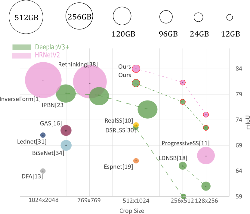
Figure 1: Graphical comparison of performance and resolution of prevalent models trained on the Cityscapes dataset [5]. Size of the circle represents the required GPU memory for training. Dashed lines connects equally-setup models trained at different resolutions.

Recent semantic segmentation proposals have relied on ever-larger and varied datasets; and high-performance hardware such as Graphical-Processing-Units (GPUs). Hardware advances allowed training using full-resolution images with larger batch sizes [26], and employing resource-expensive regional losses [36]. In fact, the former has been proved to be a binding factor for getting state-of-the-art performance (e.g., see HRNetV2 in Figure 1). However, training with full-resolution images requires high computational and storage resources [31]. This hindrance creates a huge barrier for budget-constrained research, thus limiting the development of competitive proposals to the availability of large computation facilities. For example, a high-end 32GB GPU is required to train a recent multi-scale method with a batch size of one full-resolution image [26] from the Cityscapes benchmark [5]. It is commonly agreed that larger batch sizes are crucial to increase semantic segmentation performance [37], e.g., improvements over 300% are obtained by increasing batch sizes from 2 to 8 [15]. The setups for top-performing methods range from 4 [14] to 50 [2] high-end GPUs, keeping away a large part of the scientific community from competitive research in the topic. To operate in resource-limited setups, lightweight methods have been proposed to counterbalance the resource requirements by reducing the number of parameters. This enables the use of mid-range GPUs, generally at the expense of performance. Examples of these methods are Lednet [31], DFA [13], GAS [16], Espnet [19], BiSeNet [34] and RealSS [10], whose trade-off between performance and resources is depicted in Figure 1.

Moreover, semantic segmentation methods can make use of cropped and down-sampled versions of the dataset images [14, 38], as employing such techniques diminishes the required resources. However, it becomes complicated disentangling the method’s improvements from the downgrades introduced by the scaled data, so hypothesizing the performance at full resolution becomes difficult. Therefore, two-threaded semantic segmentation benchmarks implicitly arise from the original resolution [1, 3, 29] and the widely employed down-sampled resolution [2, 11, 23, 38]. In this regard, an often ignored phenomenon is the noise and artifacts introduced by the down-sampling strategy. Specifically, a critical issue is the misalignment between the down-sampled color and label images. On one hand, smooth down-sampling estimates are preferred for the color images over majority-filter like strategies such as nearest neighbors, as the latter are prone to create blocking artifacts, jagged edges and thin structures removals [24]. On the other hand, nearest-neighbor is the default down-sampling strategy applied on label images to maintain their integer nature, as labels are categorical values that do not define a metric space.

Besides being a required stage for budget constrained training, down- and up-sampling are also generally adopted as part of the common data augmentation pipeline composed of random image resizing and crop selection to diversify training data [1, 26, 29]. Therefore, re-scaling the input data (i.e., images and labels) is transversal to almost every modern semantic segmentation training framework, with the same misalignment implications as for down-sampling.

Based on these observations, in this paper we answer (A) the following questions:

Q1. Is it possible to employ a common down-sampling strategy for the color and label images? A: Defining soft labels allows us to employ any resize strategy to the label image, including whatever used for color.

Q2. What is the impact of employing such down-sampling strategy for model training in terms of performance? A: It produces more reliable training data, thus, presenting better performances globally and on every semantic class.

Q3. What is the limit of down-sampling, i.e., how much can we reduce the input size without a significant drop in performance? A: The performance is tightly correlated to the information preserved by the down-sampling. Models start dropping performance with scale reduction. Scales below $\frac{1}{4}$ drastically reduce the information and performance.

Our best result obtains better performance using down-sampled versions of the trained images to that obtained by state-of-the-art methods using full-resolution images (see models labeled as Ours in Figure 1), also requiring significantly less computational resources. To our knowledge we are the first studying this simple yet effective approach. In practice, compared to the model using most resources—i.e., DeepLabV3+ on half resolution that employs 50 GPUs of 24 GB each to be trained for the Cityscapes dataset [2], our framework using the same architecture trained using a single Titan RTX GPU is able to outperform this model by a 3% using a quarter of the resolution and requiring less than 12GB of memory, and by a 7% using the same resolution, less than 24GB of memory, and a batch size of only 2 images.

2 Related work

Building up from Fully Convolutional Networks [17], significant advances have been made in semantic segmentation along the recent years. These are mainly focused on improving performance [2, 29] and inference speed [19, 33].

To extract fine details, semantic segmentation methods tend to present low output strides at the cost of reducing the receptive field of the network. To counteract the small receptive fields, Pyramid Pooling is employed to extract information at multiple scales [2] . DeepLab [2] employs atrous convolutions with different levels of dilation to generate features with multiple receptive fields. However, Pyramid Pooling has been recently discarded due to its fixed square context regions (pooling and dilation are typically applied in a symmetric fashion), and replaced by relational context methods, such as HRNetV2 [29], which employs attention to learn the relationships between pixels. Therefore, not being bounded to square regions [29] at the cost of a larger computational complexity [1, 26, 35, 38]. These fine details (specially edges) strongly overdrive the loss of semantic segmentation methods [1, 36] (see Figure 2). Edge information is usually biased by the down-sampling strategy, producing unstable cues for learning. Region-based losses [36] handle this instability by aggregating information from both sides of the edges. This comes, however, at the cost of increasing the computational requirements linearly with the size of the neighbourhood employed [36].

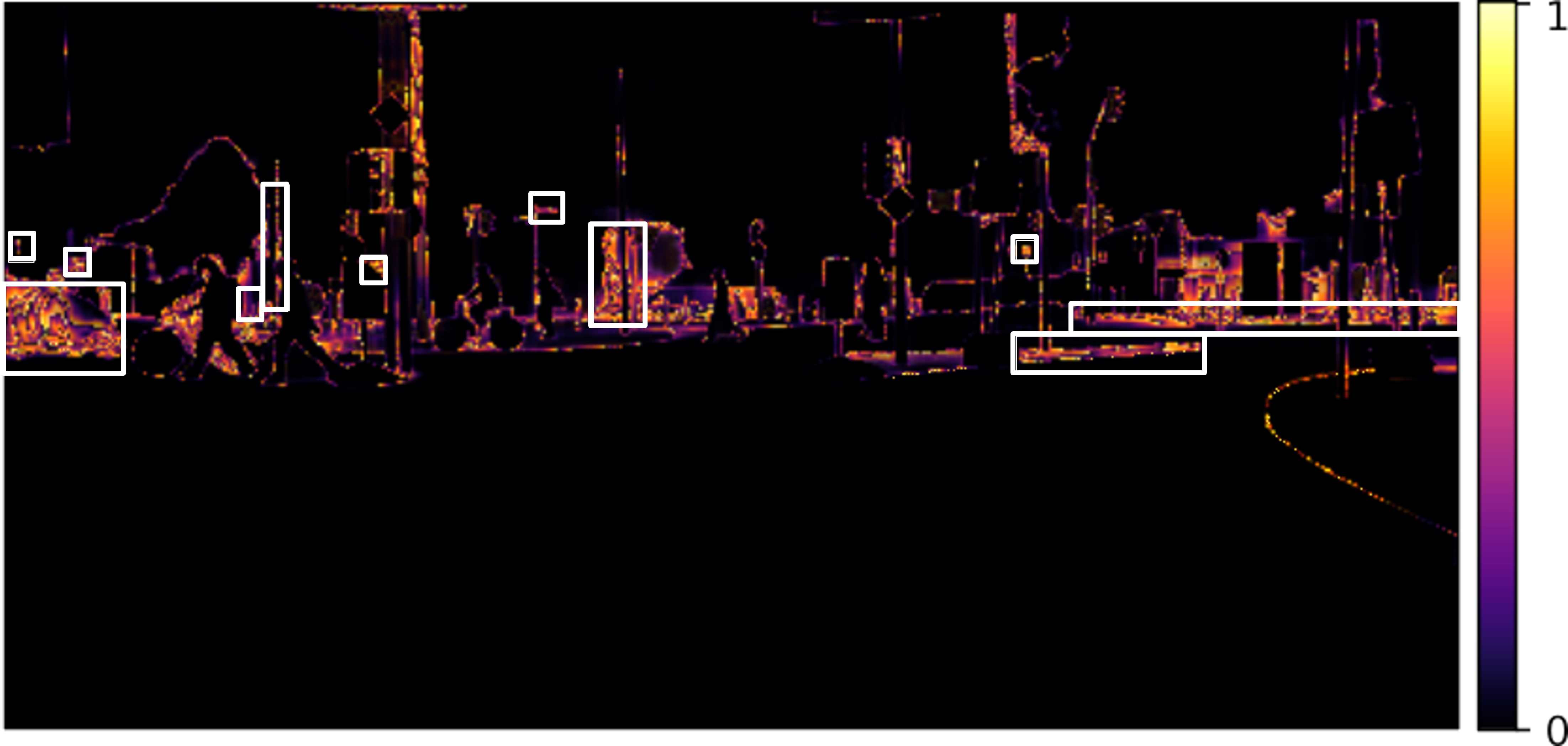
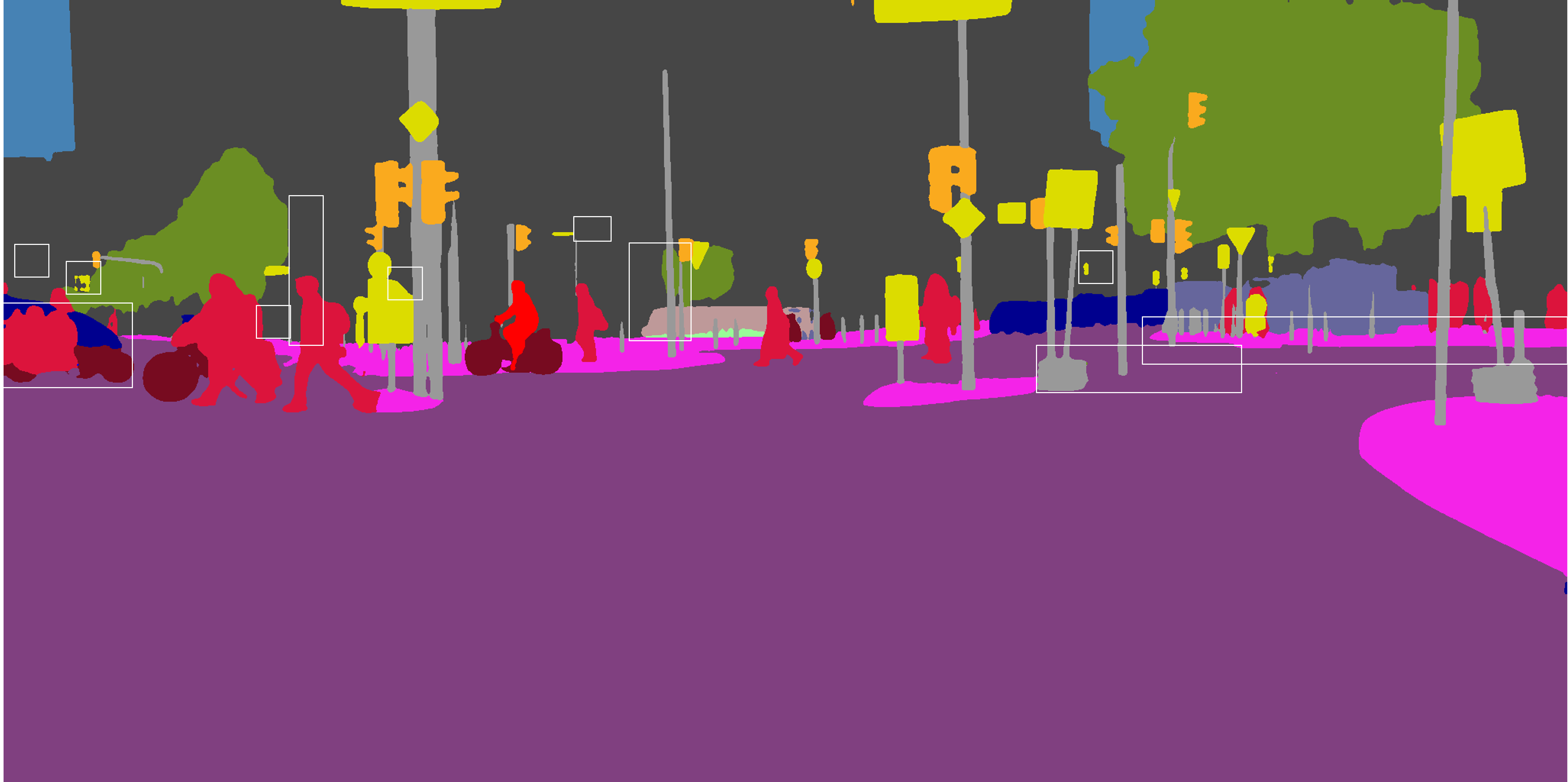
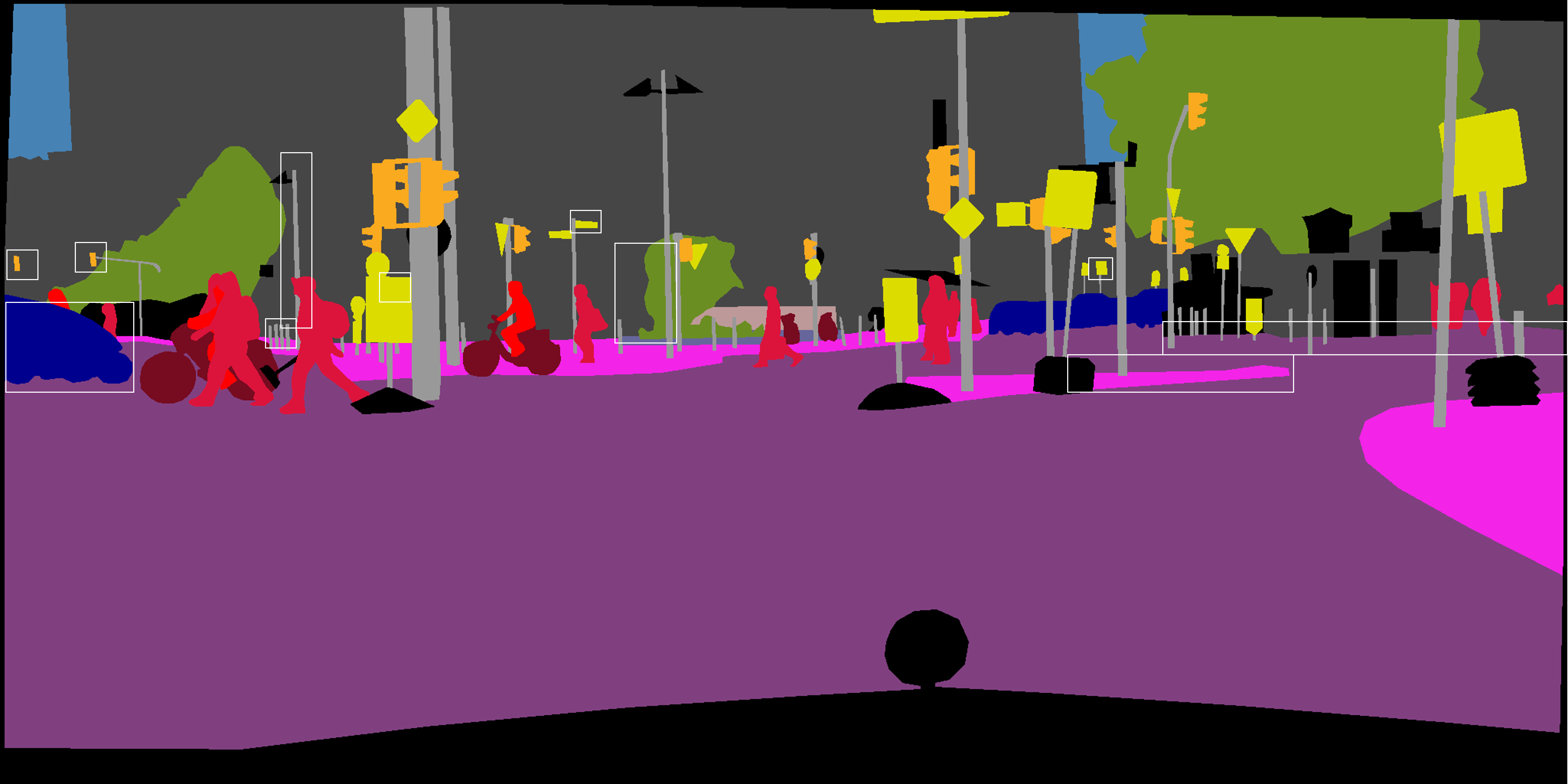
Figure 2: Per-pixel cross-entropy loss maps for the HRNetV2 model trained with a NN downsampling [29] (top). Loss is normalized to the [0,1] range. In the learning process the missing of a full structure is equally penalized as edge shifting, as can be observed in the highlighted areas, by comparing the loss values in the areas where the output (bottom, left) and the ground-truth (bottom, right) segmentation maps differ. Note that a black color in the gt represents a non-trainable area.

2.1 Alignment of color and label information

To provide a common sample selection for both color and label images, down-sampling strategies based on learned sampling [18] and multi-patch division [11] have been proposed. However, the former results in the cascading of sampling errors to the segmentation model [18]. Multi-patch training frameworks are, in turn, requested to process versions of the image multiple times, with one being a regularly down-sampled version of the image to conserve the scene context and the others crops of different scaled versions of the image to conserve small-scale objects details. In practice, this framework allows to effectively train HRNetV2 using an input size of $128\times 256$. However, 85 crops per image have to be processed, thus multiple GPUs are still needed because of the required large batch sizes.

2.2 Soft label encoding

Typically in classification tasks, the ground-truth is represented by hard-labeled one-hot encoded vectors with ones in the corresponding class. Label smoothing [20] aims at improving the performance of deep learning methods by averaging the hard labels following the distribution of labels in a training scope. This smoothing acts as a regularization by preventing the network from becoming over-confident on the ground-truth labels. Müller. et. al, [20] study the impact of label smoothing and demonstrating its positive effect on generalization. Similarly, in label presentation, soft labels are used to interpolate intermediate labels between predefined categories, e.g., for human age estimation [25], depth estimation, or horizon line regression [6]. In this paper, soft-labels provide a smooth transition between labels and help conserving the information of classes defined by small objects that are prone to be removed by down-sampling.

3 Pairing color and label down-sampling

3.1 Down-sampling in semantic segmentation

Semantic segmentation is a multi-class multi-label classification problem generally defined on color images $\mathbf{x}\in\mathbb{R}^{3,H,W}$—where $W,H\in\mathbb{N}$ are the width and height of the image and define its resolution. Each color image has associated a label image $\mathbf{y}\in\mathbb{N}^{H,W}$, where each pixel is tagged as an instance of one of the $C$ possible semantic classes. As aforementioned, color and label images are commonly down-sampled due to resource constraints, image resolution alignment, or data augmentation. Formally, the high-level standard procedure for semantic segmentation, including down-sampling is defined by:

$$\begin{split}&\mathbf{x}\in\mathbb{R}^{3,H,W}\xrightarrow{d_{x}(\cdot,\gamma)}\mathbb{R}^{3,H^{\prime},W^{\prime}}\xrightarrow{G(\cdot;\theta)}\mathbb{R}^{C,H^{\prime},W^{\prime}}.\\ &\mathbf{y}\in\mathbb{R}^{1,H,W}\xrightarrow{d_{y}(\cdot,\gamma)}\mathbb{R}^{1,H^{\prime},W^{\prime}},\end{split}$$ (1)

where $d_{x}$ and $d_{y}$ are the respective down-sampling functions for color and label images, $\gamma$ is the scale factor, $W^{\prime}=\gamma\times W,\quad H^{\prime}=\gamma\times H$ is the target resolution, and $G(\cdot;\theta)$ is the semantic segmentation model whose input are the down-sampled color images. Validation is always performed on full-resolution images.

Typically, $d_{x}$ is a smooth down-sampling strategy, a common choice is the highly efficient, yet prone to aliasing and shift variant, bilinear down-sampling [9]. In bilinear down-sampling, the sampled pixel is obtained by a weighted average of the pooled pixels. Differently, the categorical nature of the label image does not allow to apply the same strategy, so $d_{y}$ typically defines a nearest-neighbour down-sampling [24]. The lack of semantic relationships between categories precludes the use of smooth down-sampling strategies on the label image [18].

Therefore, color and label down-sampling strategies are unpaired. This generates discrepancies that are forced to be learned and memorized by the model. In fact, these discrepancies have been shown to dominate the learning attention in the last critical training epochs [1]. Remarkable effects of these discrepancies are the shape modification of inter-class boundaries (see road and sidewalk in Figure 3), the hallucination of gaps in continuous structures (see pole in Figure 3), and the elimination of small structures (see wall in Figure 3). Together, these effects affect the quantity and quality of the training data, as illustrated in Figure 3. As an example, the training a state-of-the-art model [29] with images down-sampled to a $\frac{1}{16}$ of the original resolution, results in mIoU performances of 0.3, 3.1 and 0.8 for the fences, bikes and motorcycles semantic classes. These values represent more than a 98% drop in performance compared to those obtained when training with half-size or full-resolution images [1, 14].

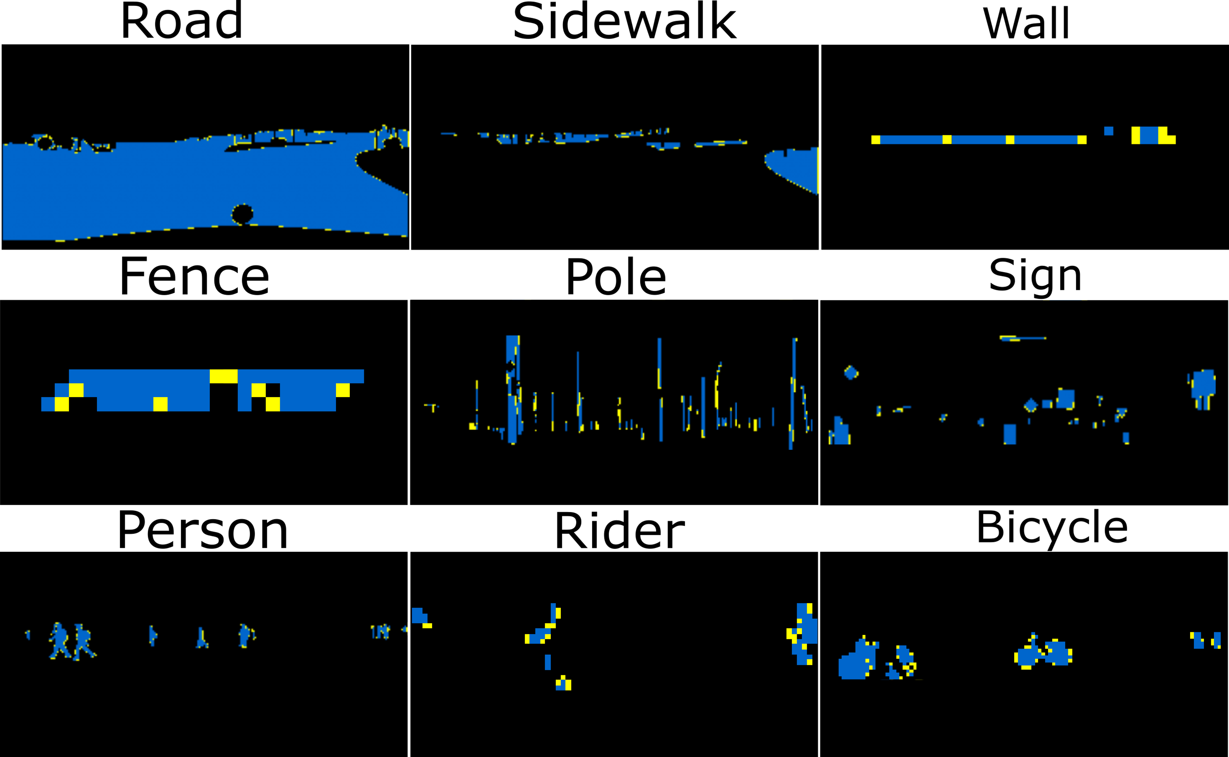
(a) Per-class visual comparison of retained information for nearest-neighbour (blue), and our soft-label (blue and yellow) after a $\frac{1}{8}$ down-sampling of the label image in Figure 2. Note the creation of jagged edges (step-like borders of blue areas) and gaps (discontinuities in blue areas).

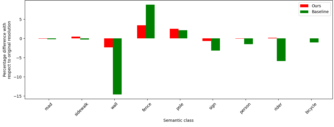
(b) Comparison of the percentage difference after a $\frac{1}{8}$ label image down-sampling for nearest neighbour (Baseline), and soft-label (Ours) strategies. Positive (Negative) values indicate label information gain (loss).

Figure 3: Generated artifacts and information conservation of nearest-neighbour and the proposed down-sampling strategies.

3.2 Proposed down-sampling strategy

To pair the down-sampling strategies for the color and the label images, we first change the representation of the categorical information in the label image to a one-hot encoding version [22], which is shaped into the $H\times W\times C$ binary matrix $\mathbf{\hat{y}}$. This matrix has ones in the spatial coordinates of the $c$-planes indicated by the class values at the same spatial coordinates in the label image.

For instance, for a pixel $(h,w)\in H\times W$ with label $\mathbf{y}_{h,w}=c$, its one-hot encoded representation is:

$$\mathbf{\hat{y}}_{h,w}=\left\{\mathbf{\hat{y}}_{h,w}^{k}\right\}_{k=1}^{C}\left\{\begin{array}[]{ll}\mathbf{\hat{y}}_{h,w}^{k}=1,k=c\\ \mathbf{\hat{y}}_{h,w}^{k}=0,elsewhere.\end{array}\right.$$ (2)

By means of this representation, rather than performing a weighted average of the corresponding sampled pixels as for the color image, one can estimate the proportion of each class in the set of labels corresponding to the pixels in the down-sampling region. Thereby, defining a vector of soft-labels for each pixel to be down-sampled.

Formally, the down-sampling on the color images can be formulated as a regional combination of the pixel values in the image $\mathbf{x}$ according to a weight function $f:\mathbb{N}^{2}\times\mathbb{N}^{2}\rightarrow\mathbb{R}$ that is applied to each pixel $(h,w)\in H\times W$ and mapped to each pixel $(u,v)\in H^{\prime}\times W^{\prime}$ of the down-sampled (target) image $\mathbf{\overline{x}}$ for each channel $k$:

$$\mathbf{\overline{x}}_{u,v}^{k}=d_{x}(\mathbf{x},\gamma)=\sum_{h,w}^{H,W}f(h,w;u,v)\cdot\mathbf{x}_{h,w}^{k}.$$ (3)

For instance, for bilinear down-sampling, $f$ is an even, decreasing function, that only depends on the distance of the target down-sampled pixel $\mathbf{\overline{x}}_{u,v}$ and the sampled pixel $\mathbf{x}_{h,w}$ in the original resolution color image. For each down-sampled pixel, its corresponding multi-class label $\mathbf{\overline{y}}_{h,w}$ is obtained by combining the one-hot encodings $\mathbf{\hat{y}}_{h,w}$ according to the employed down-sampling strategy $f(h,w;u,v)$. For example, for $\gamma=\frac{1}{2}$ bilinear down-sampling, the vector of soft-labels for pixel $(u,v)$ is obtained by:

$$\begin{split}\mathbf{\overline{y}}_{u,v}^{k}=&0.25\cdot\mathbf{\hat{y}}_{h,w}^{k}+0.25\cdot\mathbf{\hat{y}}_{h+1,w}^{k}+\\ &0.25\cdot\mathbf{\hat{y}}_{h,w+1}^{k}+0.25\cdot\mathbf{\hat{y}}_{h+1,w+1}^{k},\end{split}$$ (4)

where $h=u\cdot 2$ and $w=v\cdot 2$. Besides being aligned with the one used for the color image, the proposed down-sampling strategy enlarges the amount of information conserved from the original label image after down-sampling (see Figure 3 (b) and Figure 4). In these figures, we can observe that the widely applied nearest-neighbour does not maintain label information as down-sampling is performed.

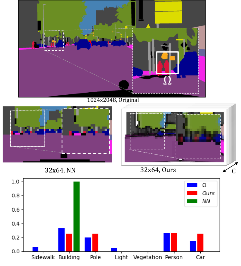
Figure 4: Visual comparison of the information conserved by different down-sampling strategies. Top-row image shows the original-resolution annotated label. Middle row represents the down-sampled results for our proposal (right) and the standard nearest-neighbour (left). Bottom row depicts the distribution of semantic classes of the highlighted region $\Omega$ in the original label image (blue) and the one obtained for the down-sampling of $\Omega$ with nearest neighbors (green) and the proposed one (red).

3.3 Controlling the impact of multi-class pixels in the training loss

Typically, semantic segmentation training is driven by the minimization of the Cross-Entropy (CE) loss between the one-hot encoding of the label image $\mathbf{\hat{y}}$, and the output probability map $G(\mathbf{x};\theta)\in\mathbb{R}^{C,H,W}$, such that $\sum_{c=1}^{C}G(\mathbf{x};\theta)_{h,w}^{c}=1\hskip 2.5pt\forall\hskip 2.5pth,w$. However, CE does not return a zero loss for soft-labels with non-zero entropy (i.e., $\forall\hskip 1.42262ptx\hskip 4.2679ptCE(x,x)=H(x)$, where $H(x)$ is the entropy of the vector x) even if the predicted labels are perfectly aligned with the ground-truth soft label. Therefore, the Kullback-Leibler (KL) divergence loss [12] is often preferred for soft-label classification [6, 25, 27, 28]:

$$\mathcal{L}_{KL}=\sum_{k,u,v}^{C,H^{\prime},W^{\prime}}\mathbf{\overline{y}}^{k}_{u,v}\cdot log\left(\frac{\overline{\mathbf{y}}^{k}_{u,v}}{G(\mathbf{x};\theta)^{k}_{u,v}}\right).$$ (5)

The employment of soft labels gives rise to a new concept of single ($\exists c|\overline{\mathbf{y}}^{c}=1$) and multi-class labels (MC). In general, one can assume that the soft labels after down-sampling are more common to be single-class instances (inner to the class region) than multi-class ones (close to the region contour). Therefore, single-class instances are prone to be easier to learn and—under a curriculum paradigm, their learning may help that of multi-class ones. However, due to the imposed nearest-neighbour sampling on the ground-truth labels, semantic edges have been analyzed to dumper semantic segmentation performance [36]. As a counter-measure, regional losses have been proposed to reduce the impact of the loss of edges [1, 36]. We analyze the impact of MC pixels in Section 4.2.

4 Experimental results

4.1 Setup

Datasets

We evaluate our proposal using Cityscapes [5], which is an urban scene dataset with $1024\times 2048$ images (3K for training and 500 for test) and 19 semantic classes. Moreover, we also consider other popular datasets to validate the generality of our proposal: Mapilliary [21] for urban scenes in another environment with 65 classes, and ADE20K [37] for general purpose segmentation with 150 classes. Further details can be found in the supplementary material.

	Down-sampling		IoU per class
	Strategy	Resolution	road	sidewalk	building	wall	fence	pole	light	sign	vegetation	terrain	sky	pedestrian	rider	car	truck	bus	train	motorcycle	bicycle	mIoU
DeeplabV3+	Nearest Neighbor	$1/8$	81.5	43.9	72.4	6.5	7.8	45.2	21.2	36.4	81.8	26.9	42.7	65.6	16.3	74.5	15.3	13.0	9.7	19.2	51.4	38.5
	Ours	$1/8$	98.0	82.8	91.0	54.0	50.1	56.0	56.2	70.4	91.6	58.8	94.3	75.8	48.3	94.0	77.2	83.9	75.5	50.7	72.2	72.7
	Nearest Neighbor	$1/4$	93.7	76.7	87.13	33.9	43.3	62.1	61.9	70.8	89.4	51.2	89.8	79.2	53.7	92.0	41.6	69.9	47.4	47.9	73.1	66.6
	Ours	$1/4$	98.3	85.9	92.7	58.0	60.2	64.3	67.3	76.8	92.6	64.1	94.9	80.9	60.3	95.2	80.4	86.8	78.4	62.8	76.2	77.7
	Nearest Neighbor	$1/2$	97.5	82.2	91.5	43.6	58.6	65.9	69.8	77.9	92.1	58.5	94.2	82.1	62.4	94.8	71.7	87.5	75.5	64.1	76.4	76.1
	Ours	$1/2$	98.3	86.8	93.4	61.6	66.4	70.0	73.5	81.5	93.2	64.2	95.4	84.8	68.3	95.4	84.8	91.7	83.5	71.2	79.9	81.3
HRNet	Nearest Neighbor	$1/8$	88.5	59.5	82.9	18.6	14.7	50.7	56.5	73.1	85.0	36.0	63.4	65.6	32.1	88.0	31.5	57.3	37.4	31.7	54.9	54.1
	Ours	$1/8$	98.3	85.6	91.6	54.5	52.5	58.1	65.8	75.5	91.9	66.8	93.6	78.0	55.8	94.8	82.3	85.0	65.8	61.5	73.2	75.3
	Nearest Neighbor	$1/4$	96.7	78.6	91.0	42.1	50.4	62.7	68.9	79.0	91.3	59.9	92.9	77.0	54.0	92.1	60.1	72.5	68.7	43.3	72.7	71.3
	Ours	$1/4$	98.7	88.3	93.8	61.4	72.2	70.1	74.1	82.6	93.2	68.7	95.4	83.4	66.0	96.0	89.5	93.0	82.7	68.8	79.3	82.0
	Nearest Neighbor	$1/2$	98.3	86.9	93.2	66.9	66.4	68.8	76.3	83.3	92.3	59.3	92.8	83.6	65.8	95.6	84.5	88.7	78.4	63.4	79.3	80.5
	Ours	$1/2$	98.8	89.7	94.4	70.0	74.4	73.5	78.1	85.4	93.5	70.5	95.8	85.9	71.0	96.3	86.2	93.6	87.9	76.6	81.5	84.4

Table 1: Per-class and overall performance comparison for the Cityscapes validation set. Two architectures have been trained (DeepLabV3+ and HRNet) with the label down-sampling (nearest-neighbour) and the proposed one using soft-labels.

Evaluation metrics

We adopt the default semantic segmentation performance measure, the PASCAL VOC per-class Intersection over Union (IoU) [7], to quantify the similarity between the model prediction and the annotations. It is defined as $IoU={TP}/{(TP+FP+FN)}$, where TP, FP and FN stand for, respectively, True Positives, False Positives and False Negatives. As a global performance evaluation, we use the overall mean IoU averaging IoU values for all classes (mIoU). All the reported models have been evaluated using full-resolution images in the test stage.

Explored semantic segmentation architectures

For the Cityscapes and Mapilliary datasets, we conduct ablation studies on two high-performance architectures: HRNetV2-48 [29] and DeeplabV3+ [2] with a backbone of WideResNet-38 aligned with [23]. For experiments in the ADE20K dataset, we employ SegFormer (MiT-B2) [32]. We compare our strategy against 13 (contar sin 18) state-of-the-art approaches, 12 of them employing nearest neighbour down-sampling for budget-constrained ([8, 19, 30]) and unconstrained ([1, 2, 3, 4, 14, 23, 29, 35, 37]) resources. Furthermore, we also consider [18] that explicitly learns a down-sampling alternative to nearest neighbours.

Implementation details

We employ Pytorch as our deep learning framework. As GPU hardware, experiments are carried out either on a single GeForce Titan 12GB or on a single Titan RTX 24GB. We employ the maximum batch size for each GPU: 6 and 20 for the 12GB GPU (input resolution of $256\times 512$ and $128\times 256$, respectively), and 3 and 12 for the 24GB GPU (input resolution of $512\times 1024$ and $256\times 512$, respectively). Our model is trained using SGD optimizer with momentum of $0.9$ and weight decay of $10^{-4}$ following [26]. No extra data is employed for any reported result, being restricted to the available train and test sets of each dataset. The code and setup for reproducibility are available at $<$hidden for revision to preserve anonymity$>$.

4.2 The paired down-sampling enables effective and efficient semantic segmentation training

We validate our proposal for the crop-based data augmentation widely used in semantic segmentation [1, 14, 26]. This augmentation defines an input resolution for training (i.e., crop size), performs random resizing of the original image and label data for all batch samples, and later extracts training crops from resized images. This resizing ranges from half to twice the defined crop size. We apply our down-sampling strategy to the resizing of label images, and we consider three down-sampling factors relative to the original training data resolution: $\frac{1}{8},\frac{1}{4},\frac{1}{2}$. Therefore, we train three models for each explored architecture (DeeplabV3+ and HRNetV2). As baseline for comparison, we use the default unpaired down-sampling strategies for color (bilinear) and label images (nearest-neighbors).

	Resolution	TTT	Memory	mIoU
	$128\times 256$	1	12GB	75.3
HRNetV2	$256\times 512$	3.4	12GB	82.0
	$512\times 1024$	7	24GB	84.4
	$128\times 256$	1	12GB	72.7
DeeplabV3+	$256\times 512$	3.4	12GB	77.7
	$512\times 1024$	15.5	24GB	81.3

Table 2: Relative total training time (TTT) comparison of the image resolutions used for training. mIoU is computed on the Cityscapes validation set.

Performance comparison

Table 1 compiles the per-class performances for all the trained models. Both the global (mIoU) and all the per-class performances (IoU) of the models trained using the proposed down-sampling strategy are higher than those of their respective baselines. It is noteworthy that the performance of the $\frac{1}{4}$ models using the proposed down-sampling strategy is higher than those of their respective $\frac{1}{2}$ baseline models. Gains in performance are larger for thin classes (fence, pole, traffic light) and low represented classes (e.g., wall). Figure 5 depicts qualitative results for different training input resolutions. Note how as the training input decreases its resolution, so does the models capability of discerning further finer details. In the supplementary material, we include an statistical analysis on the correlation between the nature of the classes and the gains in performance.

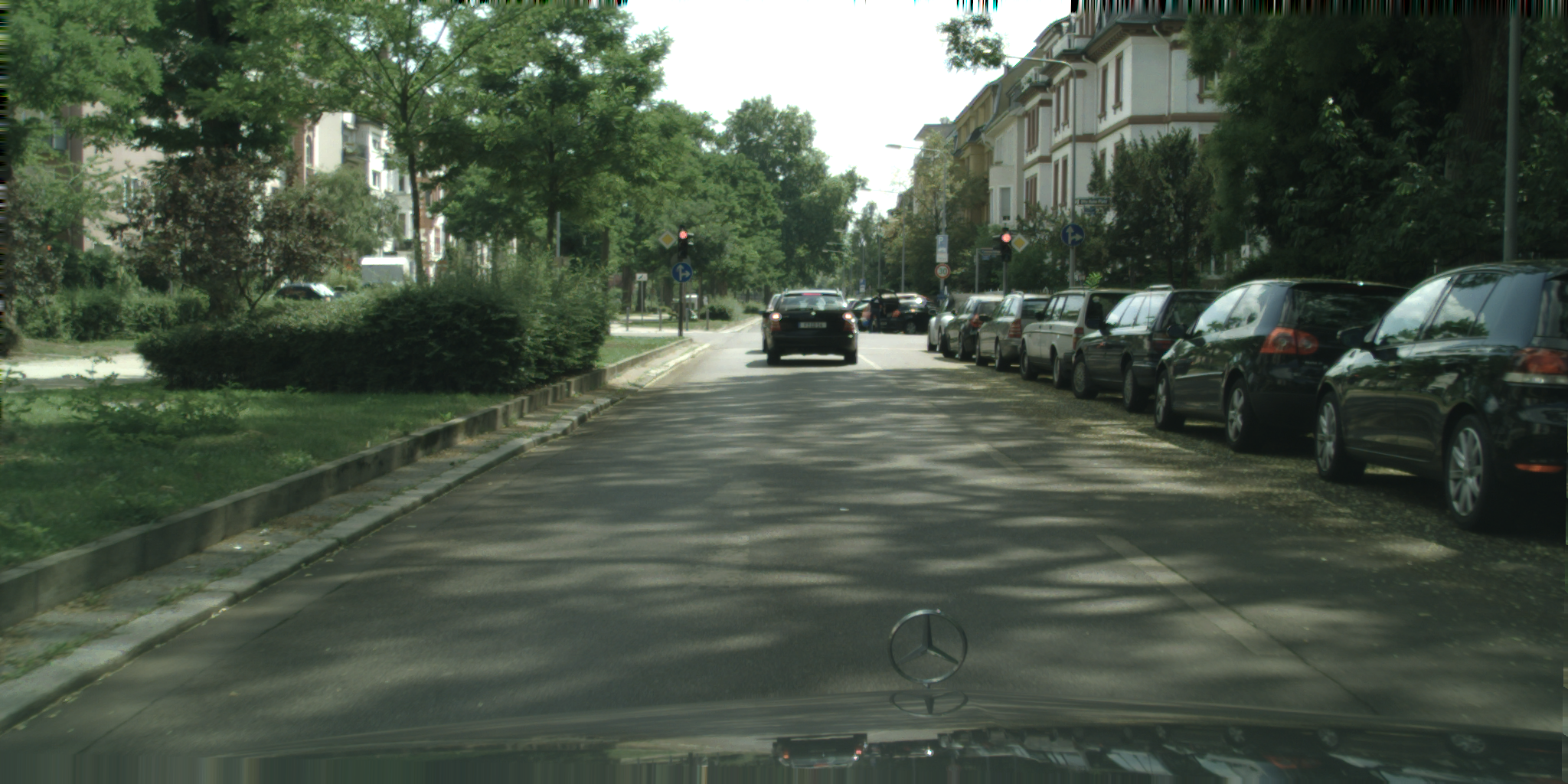
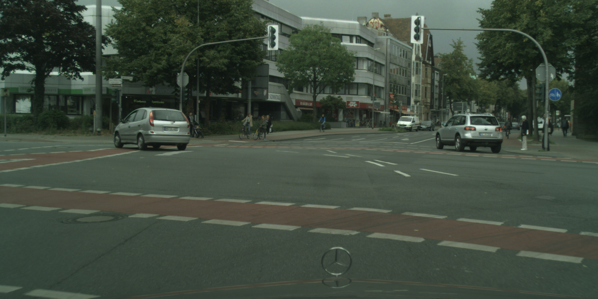
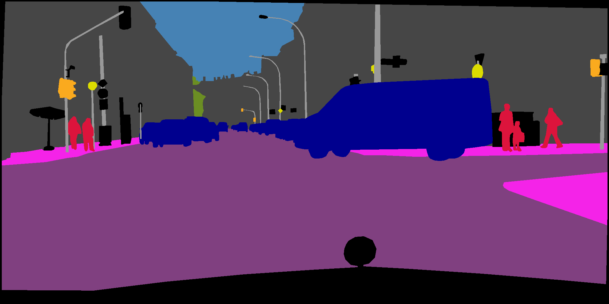
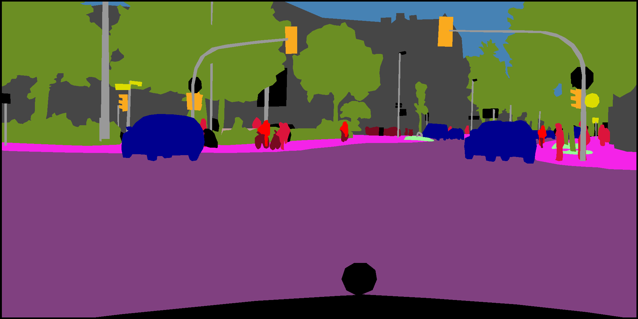
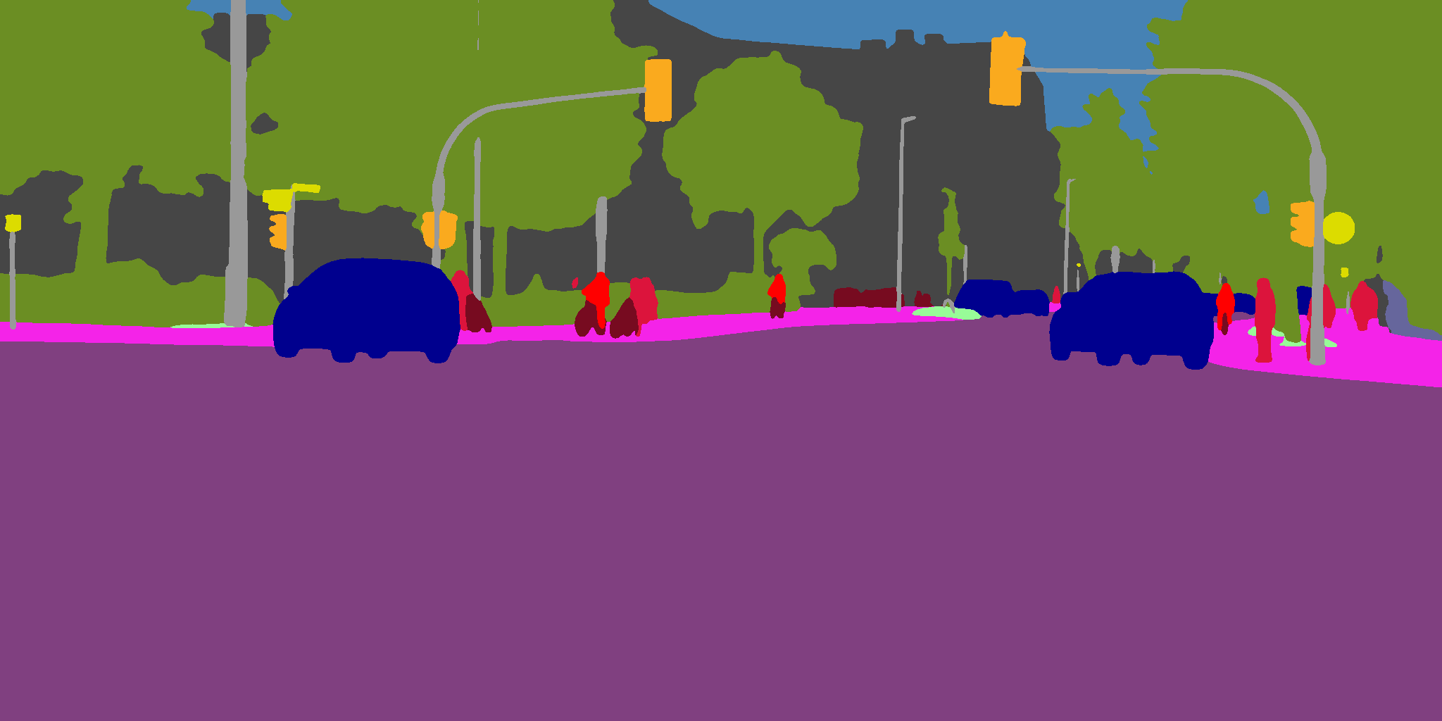
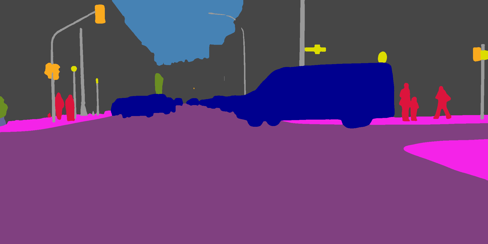
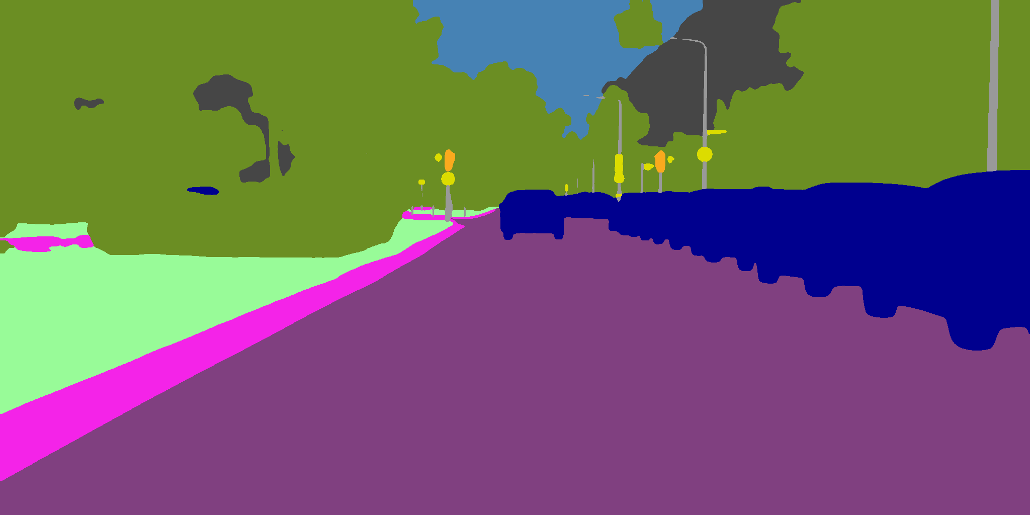
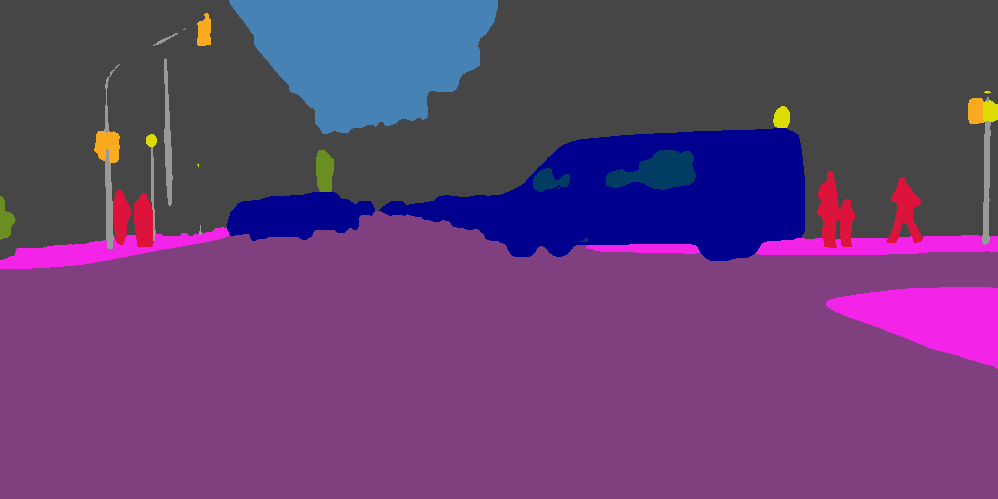
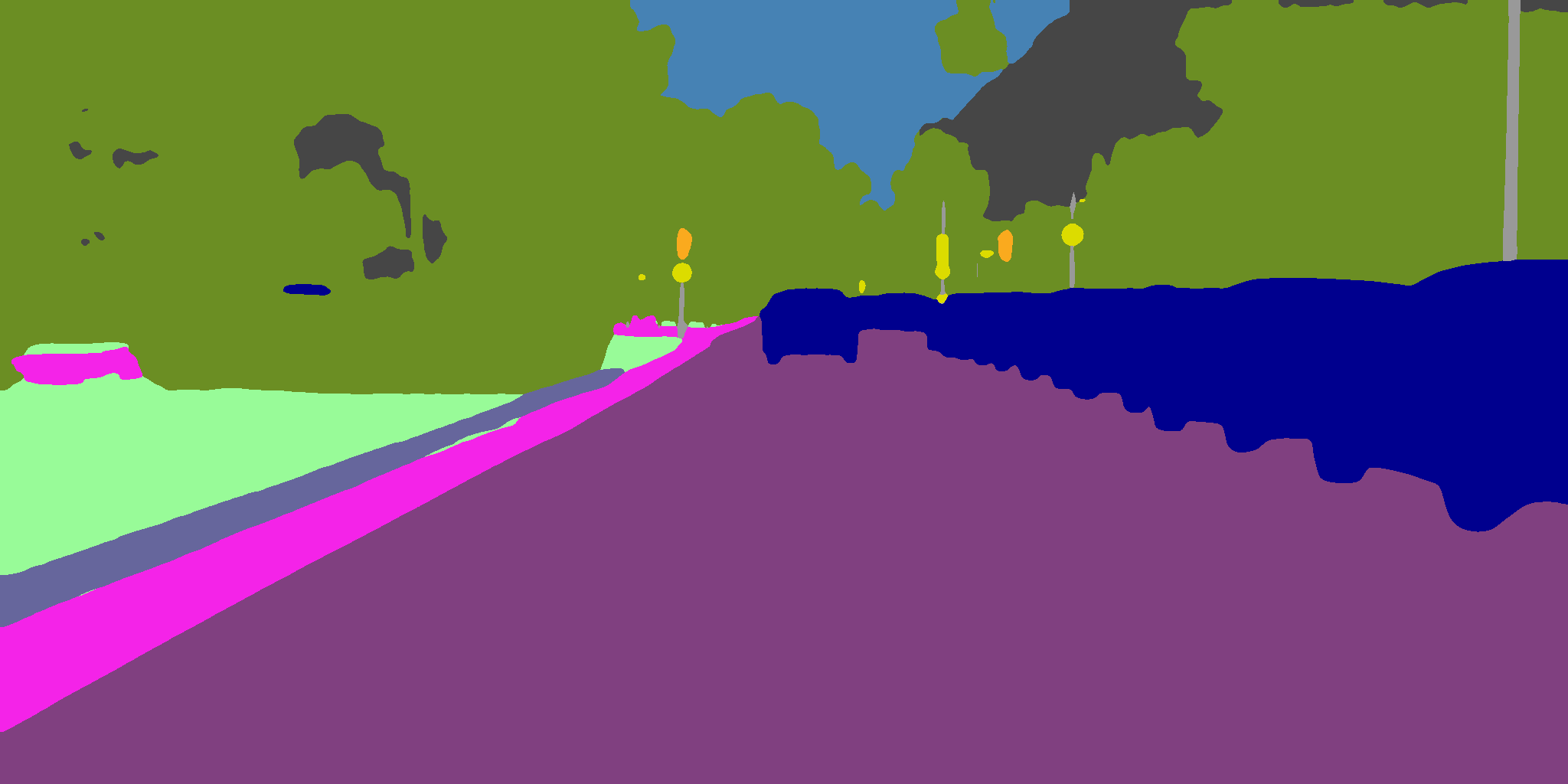
Figure 5: Qualitative comparison of our models trained on different input resolutions. First and second rows represent the color and label images. The third, fourth and fifth rows illustrate the outputs of HRNetV2 models trained with input resolutions of $\frac{1}{2},\frac{1}{4},\frac{1}{8}$ respectively.

Memory requirements

The highest performances of semantic segmentation models is usually obtained by training with large resolutions, which lead to high computational resources in terms of memory consumption and computation time. In Table 2, we present the time and memory requirements to train the models reported in Table 1. The advantages of the proposed strategy is clearly seen as resources are signficantly decreased. For instance, for the $1/8$ resolution models, the training is over 7 times faster than that of the $1/2$ resolution ones, while maintaining more than 90% of the mIoU performance at the $1/2$ resolution.

On the advantages of using multi-class pixels

We quantify the effect of considering multi-class pixels by only computing the loss over the single-class pixels or both the single and multi-class pixels. These loss setups are used to drive training processes on the Cityscapes training images at different resolutions using the proposed strategy or the nearest neighbor one. Note that the latter only generates single-class pixels. Reported results in Table 3 suggest that the main benefits of the proposed strategy emerge from the down-sampling proposal: as the gain obtained by MC is narrower than the overall gain obtained when the down-sampling strategy is changed. However, empirical results suggests that MC pixels do have a positive impact in the model performance for bigger input resolutions. This is specially remarkable for the highest resolution explored (half-resolution), where our soft labels are capable of conserving all the information of the labels.

Resolution	Down-sampling	MC	mIoU
$128\times 256$	Nearest Neighbors	$\times$	54.1
	Ours	$\times$	76.0
	Ours	✓	75.3
$256\times 512$	Nearest Neighbors	$\times$	71.3
	Ours	$\times$	80.7
	Ours	✓	82.0
$512\times 1024$	Nearest Neighbors	$\times$	81.6
	Ours	$\times$	82.1
	Ours	✓	84.4

Table 3: Ablation study on the down-sampling strategy employed on the semantic maps and the employed loss for training. Results from training a HRNetV2 [35] on the Cityscapes validation set. MC indicates if the loss takes into account multi-class pixels. Bold indicates best results.

4.3 The proposed down-sampling strategy achieves state-of-the art performance using at most 24 GB of GPU memory

Tables 4 and 5 compare the models trained using label images down-sampled with the proposed strategy (Ours) with those for top performing state-of-the art approaches in the Cityscapes validation set. Specifically, Table 4 our models and alternative lightweight approaches for the case of limited resources (i.e., restricted to 12GB GPU memory). Our best model (HRNetV2) outperforms the current state of the art [30] by an 11%. Qualitative examples can be found in the supplementary material.

Model	Resolution	mIoU
LDNSB[18]	$128\times 256$	62.0
DSRLSS[30]	$256\times 512$	59.2
LDNSB[18]	$256\times 512$	65.0
Espnetv2[19]	$512\times 1024$	66.2
DSRLSS[30]	$512\times 1024$	66.9
Mscfnet[8]	$512\times 1024$	71.9
HRNetV2-Ours	$128\times 256$	75.3
HRNetV2-Ours	$256\times 512$	81.5

Table 4: 12GB-constrained setup performance comparison of semantic segmentation models on the Cityscapes validation set. Reference methods’ performances as reported in their papers. Bold indicates best.

Table 5 depicts the comparison with semantic segmentation approaches without restrictions on the resources employed. Due our resource availability of a single 24GB GPU, we only report half-resolution performance for our model employing, as full-resolution training requires at least a 32GB GPU for a batch size of 1. We outperform every selected approach with substantially lower memory requirements, regardless of the context method the architecture employs. Furthermore, our proposal has lower complexity—in terms of implementation effort and setup. In contrast, approaches [1, 14] and [38] rely on regional losses, while [4] and [1] require the use of auxiliary networks to either post-process each pixel classification or detect edges and shifts between ground-truth and prediction. As a result, our proposal stands out as a more efficient and effective solution despite our constrained training setup. Figure 6 visually compares the performance of the state-of-the-art semantic segmentation model OCR [35] with our best model, both using same architecture, HRNetV2. Note how our model is less prone to generate semantic gaps in structures and can segment better the finer details of the image. Additional visual comparisons with different models can be found in the supplementary material.

		Training Hardware		Training Hyperparameters
Context method	Model	#GPUs	GB/GPU	BS	Resolution	mIoU
Pyramid	IPBN[23]	4	24	12	$872\times 872$	79.4
Pooling	PanopticDL[3]	32	32	32	$1024\times 2048$	81.5
	DeeplabV3+[2]	50	24	$>$16*	$513\times 513$	79.6
2-7	Deeplab-Ours	1	24	3	$512\times 1024$	81.3
Relational	HRNetV2[29]	4	32	12	$512\times 1024$	81.6
context	OCRnet[35]	4	32	8	$769\times 769$	81.8
	DHSS[14]	4	40	8	$512\times 1024$	83.4
	Rethinking[38]	8	32	8	$768\times 768$	81.1
	PPC[4]	8	32	16	$512\times 1024$	81.4
	InverseForm[1]	16	32	16	$1024\times 2048$	82.6
2-7	HRNetV2-Ours	1	24	3	$512\times 1024$	84.4

Table 5: Unconstrained comparison of state-of-the-art semantic segmentation models on the Cityscapes validation set. Reported training setup depicts the stated number of GPUs and memory per GPU employed for training. When batch size (BS) is not explicitly reported ‘*’, we provide the reported minimum batch size required. Bold indicates best results per context method.

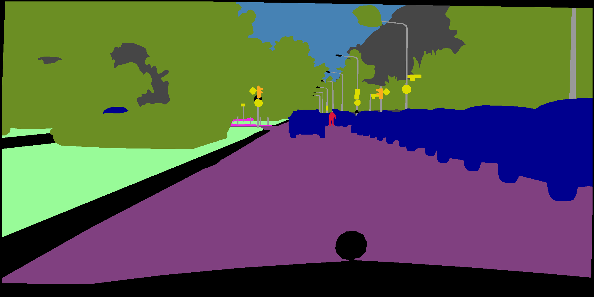
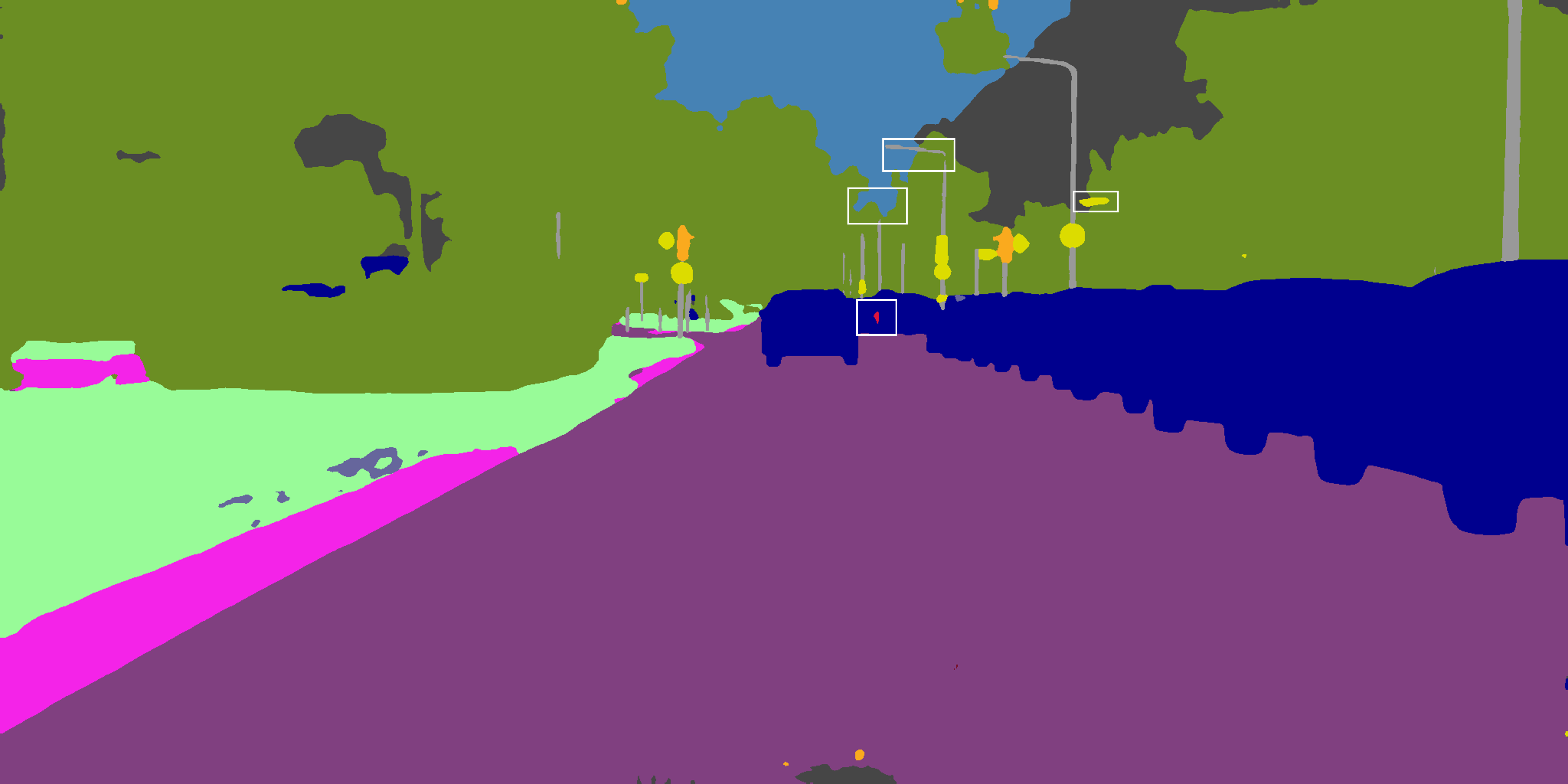
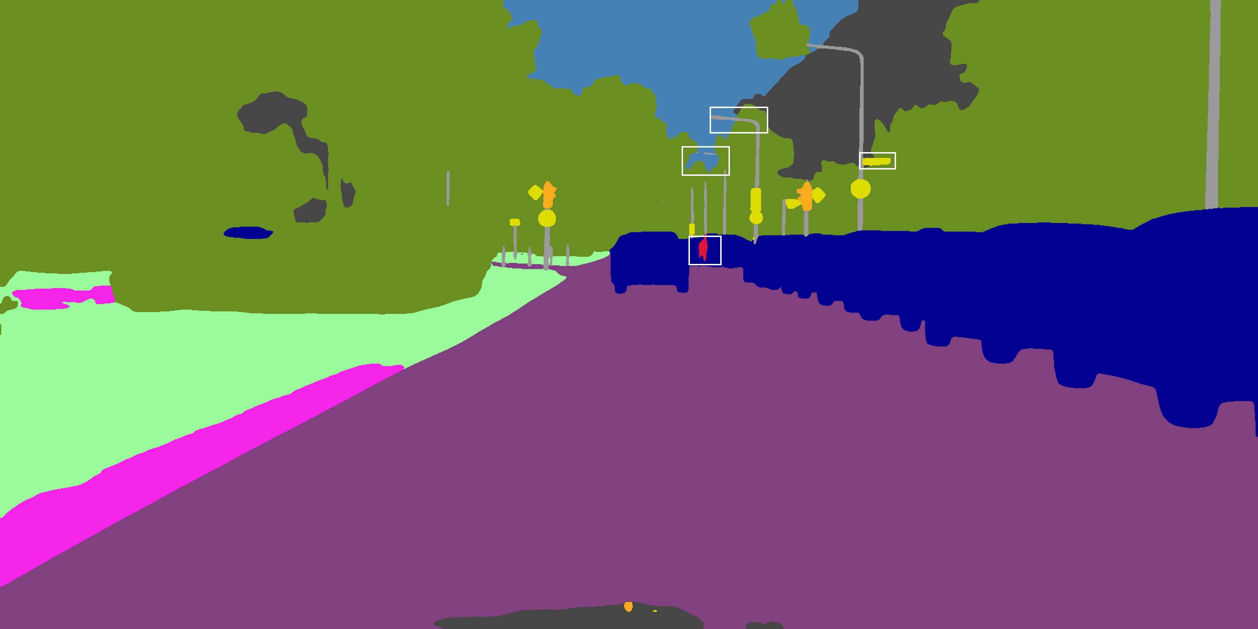
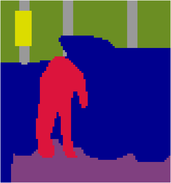
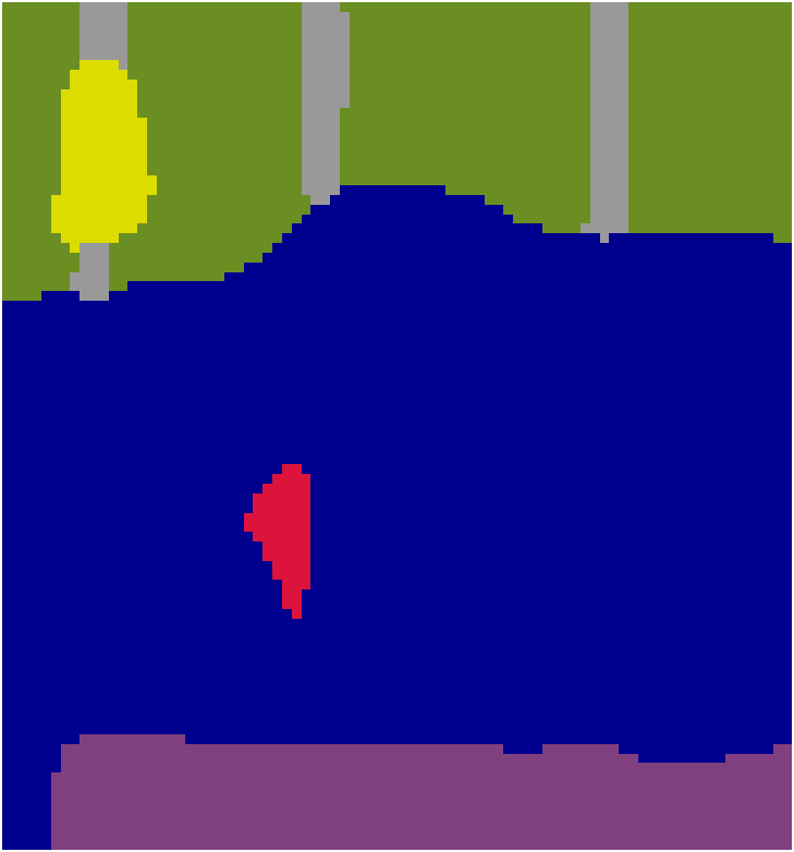
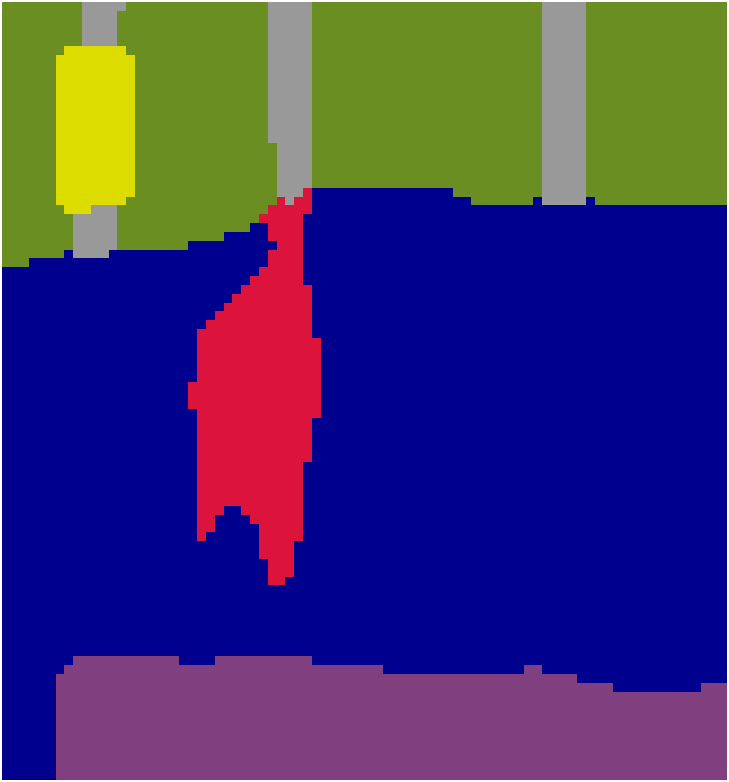
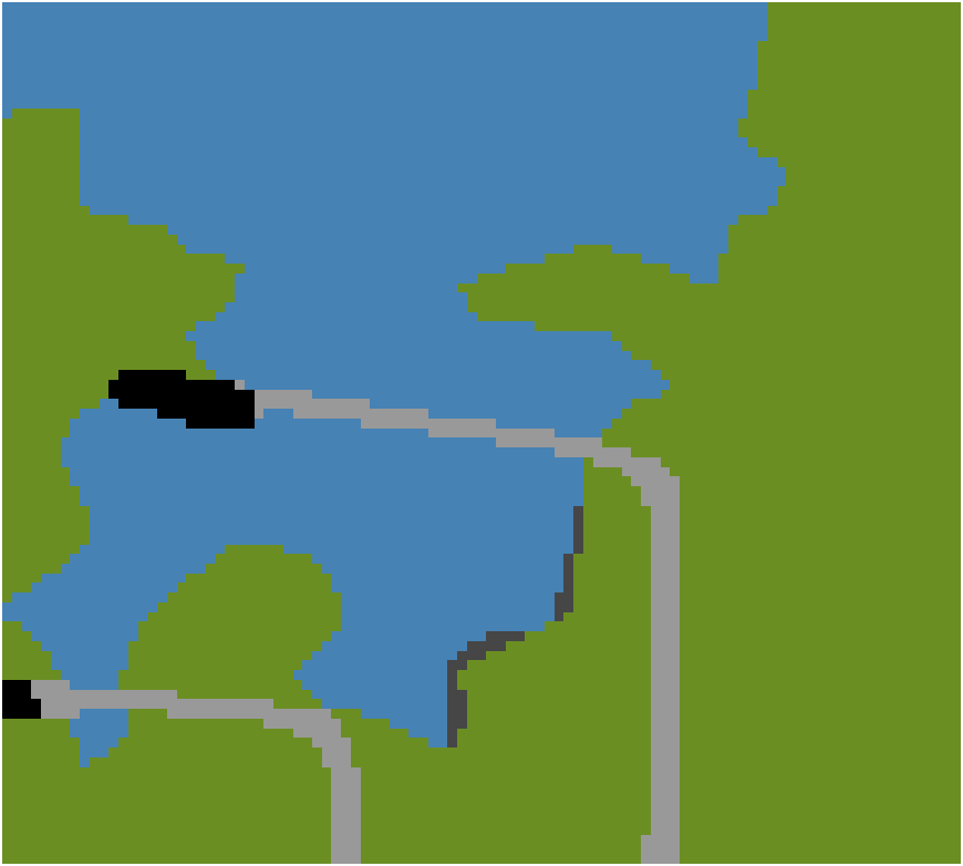
Figure 6: Detailed visual comparison of OCR [35] and our best model. First two columns of the first row represent the color and label images respectively. Third and fourth columns of the first row represent OCR and our segmentation map respectively. Second row illustrates crops of the GT, OCR model and our model.

4.4 The advantages of the proposal are transferred to other datasets

Differently to the Cityscapes dataset, alternative semantic segmentation datasets (e.g., Mapilliary and ADE20K) are composed of images with variable resolutions. However, the data augmentation strategy previously discussed provides a homogeneous input for model training. For the ADE20K dataset, we here explore the effect of using the proposed down-sampling strategy in a more general sense than just to reduce input resolution, performing up-sampling when the selected crop size is bigger than the image. Including our strategy in the training of the architecture SegFormer [32], notably benefits the test performance, see Table 6. Moreover, in Table 7 we report performance results by the same setup used for our best performing Cityscapes model with the HRNetV2 architecture, when trained and evaluated on the Mapilliary dataset. Comparing this model with a reference one that uses the same architecture [35], our down-sampling strategy provides a 7% global increase in performance, requiring 10 times less GPU memory.

	Training Hardware
Model	#GPUs	GB/GPU	mIoU
DeeplabV3+[2]	50	2	44.1
MaskFormer[14]	8	32	44.5
OCRnet[35]	4	32	45.5
SegFormer[32]	8	32	46.5
SegFormer-Ours	1	24	48.3

Table 6: Performance and training hardware comparison of state-of-art semantic segmentation frameworks on the ADE20K validation set trained on Full Resolution.

4.5 On conserving all the information.

In the previous sections, we have validated the benefits of using a soft-label encoding of information to pair the down-sampling strategy used for the label image with that used for the color one. However, the use of soft labels may allow to conserve all the information for any down-sample factor by considering the labels of all the pixels in the down-sampling region in the encoding. Thereby, the entropy of the class distribution in the down-sampling region and that of the resulting soft-label encoding will be the same. In our experiments, this is only the case for half-resolution down-sampling. For the other factors, only some pixels in the down-sampling region are considered by the bilinear strategy. Using the full-potential of the proposed soft-label encoding is interesting, but entails the definition of a paired down-sampling strategy for the color image. This is a major challenge that needs to be explored in future work as a soft color encoding would require a large input structure—albeit this is prone to be sparse.

	Training Hardware
Model	#GPUs	GB/GPU	mIoU
DeeplabV3+[2]	50	24	47.7
OCRnet[35]	4	32	50.8
MaskFormer[4]	8	32	53.1
HRNetV2-Ours	1	24	54.4

Table 7: Performance and training requirements comparison of state of art semantic segmentation frameworks on the Mapilliary validation set trained on Full Resolution.

5 Conclusion

In this paper we propose a novel and simple framework for training semantic segmentation models under different resolutions, which can be easily included into any existing framework with minor modifications. By using a soft-label encoding of the labels after down-sampling, we manage to pair the down-sampling strategies used for the color and label images, aligning their information and precluding the learning of discrepant information during the training of semantic segmentation models. Extensive experimentation is conducted to validate the effectiveness of our proposal. Experimental results suggest that the use of this strategy culminates in the learning of models that surpass by over a 88% their respective baselines using the same architecture, data and setup but trained adopting the default nearest neighbor down-sampling. Furthermore, in the explored setups, the proposed framework can be fully trained using at most a single 24GB GPU, generating models which performance is better than the state of the art for all explored input resolutions. Moreover, our models trained on half-resolution images get better performance than reference state-of-the-art models trained on full resolution and using substantially larger batches than us. We believe this framework has the potential to expand the effective validation of new research conducted at budget-constrained research facilities for semantic segmentation.

References

- [1] Shubhankar Borse, Ying Wang, Yizhe Zhang, and Fatih Porikli. Inverseform: A loss function for structured boundary-aware segmentation. In IEEE Conf. Comput. Vis. Pattern Recognit. (CVPR), pages 5897–5907, 2021.
- [2] Liang-Chieh Chen, Yukun Zhu, George Papandreou, Florian Schroff, and Hartwig Adam. Encoder-decoder with atrous separable convolution for semantic image segmentation. In IEEE Eur. Conf. Comput. Vis. (ECCV), page 833–851, 2018.
- [3] Bowen Cheng, Maxwell D Collins, Yukun Zhu, Ting Liu, Thomas S Huang, Hartwig Adam, and Liang-Chieh Chen. Panoptic-deeplab: A simple, strong, and fast baseline for bottom-up panoptic segmentation. In IEEE Conf. Comput. Vis. Pattern Recognit. (CVPR), pages 12472–12482, 2020.
- [4] Bowen Cheng, Alex Schwing, and Alexander Kirillov. Per-pixel classification is not all you need for semantic segmentation. In M. Ranzato, A. Beygelzimer, Y. Dauphin, P.S. Liang, and J. Wortman Vaughan, editors, Advances in Neural Information Processing Systems (NeurIPS), pages 17864–17875, 2021.
- [5] Marius Cordts, Mohamed Omran, Sebastian Ramos, Timo Rehfeld, Markus Enzweiler, Rodrigo Benenson, Uwe Franke, Stefan Roth, and Bernt Schiele. The cityscapes dataset for semantic urban scene understanding. In IEEE Conf. Comput. Vis. Pattern Recognit. (CVPR), pages 3212–3223, 2016.
- [6] Raul Diaz and Amit Marathe. Soft labels for ordinal regression. In IEEE Conf. Comput. Vis. Pattern Recognit. (CVPR), pages 4733–4742, 2019.
- [7] Mark Everingham, Luc Van Gool, C. K. I. Williams, J. Winn, and Andrew Zisserman. The pascal visual object classes (voc) challenge, 2010.
- [8] Guangwei Gao, Guoan Xu, Yi Yu, Jin Xie, Jian Yang, and Dong Yue. Mscfnet: A lightweight network with multi-scale context fusion for real-time semantic segmentation. CoRR, abs/2103.13044, 2021.
- [9] Dianyuan Han. Comparison of commonly used image interpolation methods. In Int. Conf. Comput. Science and Electronics Engineering (ICCSEE), pages 1556–1559, 2013.
- [10] Yuanduo Hong, Huihui Pan, Weichao Sun, and Yisong Jia. Deep dual-resolution networks for real-time and accurate semantic segmentation of road scenes. arXiv preprint arXiv:2101.06085, 2021.
- [11] Chuong Huynh, Anh Tran, Khoa Luu, and Minh Hoai. Progressive semantic segmentation. In IEEE Conf. Comput. Vis. Pattern Recognit. (CVPR), pages 16750–16759, 2021.
- [12] Solomon Kullback and Richard A Leibler. On information and sufficiency. The annals of mathematical statistics, pages 79–86, 1951.
- [13] Hanchao Li, Pengfei Xiong, Haoqiang Fan, and Jian Sun. Dfanet: Deep feature aggregation for real-time semantic segmentation. IEEE Conf. Comput. Vis. Pattern Recognit. (CVPR), pages 9514–9523, 2019.
- [14] Liulei Li, Tianfei Zhou, Wenguan Wang, Jianwu Li, and Yi Yang. Deep hierarchical semantic segmentation. In IEEE Conf. Comput. Vis. Pattern Recognit. (CVPR), pages 1246–1257, 2022.
- [15] Caojia Liang, Junfeng Ge, Wei Zhang, Kang Gui, Faouzi Alaya Cheikh, and Lin Ye. Winter road surface status recognition using deep semantic segmentation network. In Int. Workshop on Atmospheric Icing of Structures (IWAIS), pages 23–28, 2019.
- [16] Peiwen Lin, Peng Sun, Guangliang Cheng, Sirui Xie, Xi Li, and Jianping Shi. Graph-guided architecture search for real-time semantic segmentation. IEEE Conf. Comput. Vis. Pattern Recognit. (CVPR), pages 4202–4211, 2020.
- [17] Jonathan Long, Evan Shelhamer, and Trevor Darrell. Fully convolutional networks for semantic segmentation. In IEEE Conf. Comput. Vis. Pattern Recognit. (CVPR), pages 3431–3440, 2015.
- [18] Dmitrii Marin, Zijian He, Peter Vajda, Priyam Chatterjee, Sam Tsai, Fei Yang, and Yuri Boykov. Efficient segmentation: Learning downsampling near semantic boundaries. In IEEE Int. Conf. Comput. Vis. (ICCV), pages 2131–2141, 2019.
- [19] Sachin Mehta, Mohammad Rastegari, Linda Shapiro, and Hannaneh Hajishirzi. Espnetv2: A light-weight, power efficient, and general purpose convolutional neural network. In IEEE Conf. Comput. Vis. Pattern Recognit. (CVPR), pages 9182–9192, 2019.
- [20] Rafael Müller, Simon Kornblith, and Geoffrey Hinton. When does label smoothing help? In Advances in Neural Information Processing Systems (NeurIPS), page 4694–4703, 2019.
- [21] Gerhard Neuhold, Tobias Ollmann, Samuel Rota Bulò, and Peter Kontschieder. The mapillary vistas dataset for semantic understanding of street scenes. In IEEE Int. Conf. Comput. Vis. (ICCV), pages 5000–5009, 2017.
- [22] Kedar Potdar, Taher Pardawala, and Chinmay Pai. A comparative study of categorical variable encoding techniques for neural network classifiers. Int. Journal of Computer Applications, pages 7–9, 2017.
- [23] Samuel Rota Bulò, Lorenzo Porzi, and Peter Kontschieder. In-place activated batchnorm for memory-optimized training of dnns. In IEEE Conf. Comput. Vis. Pattern Recognit. (CVPR), 2018.
- [24] Olivier Rukundo. Evaluation of rounding functions in nearest neighbor interpolation. Int. Journal of Computational Methods, 18, 2021.
- [25] Zichang Tan, Shuai Zhou, Jun Wan, Zhen Lei, and Stan Z. Li. Age estimation based on a single network with soft softmax of aging modeling. In Shang-Hong Lai, Vincent Lepetit, Ko Nishino, and Yoichi Sato, editors, Asian Conf. Comput. Vis.(ACCV), pages 203–216, 2017.
- [26] Andrew Tao, Karan Sapra, and Bryan Catanzaro. Hierarchical multi-scale attention for semantic segmentation. CoRR, abs/2005.10821, 2020.
- [27] Eric Tzeng, Judy Hoffman, Trevor Darrell, and Kate Saenko. Simultaneous deep transfer across domains and tasks. In IEEE Int. Conf. Comput. Vis. (ICCV), pages 4068–4076, 2015.
- [28] Haoran Wang, Tong Shen, Wei Zhang, Lingyu Duan, and Tao Mei. Classes matter: A fine-grained adversarial approach to cross-domain semantic segmentation. IEEE Eur. Conf. Comput. Vis. (ECCV), pages 642,659, 2020.
- [29] Jingdong Wang, Ke Sun, Tianheng Cheng, Borui Jiang, Chaorui Deng, Yang Zhao, Dong Liu, Yadong Mu, Mingkui Tan, Xinggang Wang, Wenyu Liu, and Bin Xiao. Deep high-resolution representation learning for visual recognition. IEEE Transactions on Pattern Analysis and Machine Intelligence, pages 3349–3364, 2021.
- [30] Li Wang, Dong Li, Yousong Zhu, Lu Tian, and Yi Shan. Dual super-resolution learning for semantic segmentation. In IEEE Conf. Comput. Vis. Pattern Recognit. (CVPR), pages 3773–3782, 2020.
- [31] Yu Wang, Quan Zhou, Jia Liu, Jian Xiong, Guangwei Gao, Xiaofu Wu, and Longin Jan Latecki. Lednet: A lightweight encoder-decoder network for real-time semantic segmentation. In IEEE Int. Conf. Image Processing (ICIP), pages 1860–1864, 2019.
- [32] Enze Xie, Wenhai Wang, Zhiding Yu, Anima Anandkumar, José Manuel Álvarez, and Ping Luo. Segformer: Simple and efficient design for semantic segmentation with transformers. In Advances in Neural Information Processing Systems (NeurIPS), 2021.
- [33] Michael Ying Yang, Saumya Kumaar, Ye Lyu, and Francesco Nex. Real-time semantic segmentation with context aggregation network. Journal of Photogrammetry and Remote Sensing (ISPRS), pages 124–134, 2021.
- [34] Changqian Yu, Jingbo Wang, Chao Peng, Changxin Gao, Gang Yu, and Nong Sang. Bisenet: Bilateral segmentation network for real-time semantic segmentation. In IEEE Eur. Conf. Comput. Vis. (ECCV), pages 334,349, 2018.
- [35] Yuhui Yuan, Xilin Chen, and Jingdong Wang. Object-contextual representations for semantic segmentation. In IEEE Eur. Conf. Comput. Vis. (ECCV), pages 173–190, 2020.
- [36] Shuai Zhao, Yang Wang, Zheng Yang, and Deng Cai. Region mutual information loss for semantic segmentation. In Advances in Neural Information Processing Systems (NeurIPS), page 11117–11127, 2019.
- [37] Bolei Zhou, Hang Zhao, Xavier Puig, Tete Xiao, Sanja Fidler, Adela Barriuso, and Antonio Torralba. Semantic understanding of scenes through the ade20k dataset. Int. Journal of Computer Vision, pages 302–321, 2019.
- [38] Tianfei Zhou, Wenguan Wang, Ender Konukoglu, and Luc Van Gool. Rethinking semantic segmentation: A prototype view. In IEEE Conf. Comput. Vis. Pattern Recognit. (CVPR), pages 2572–2583, 2022.