SpikeGPT: Generative Pre-trained Language Model with Spiking Neural Networks

Abstract

As the size of large language models continue to scale, so does the computational resources required to run it. Spiking Neural Networks (SNNs) have emerged as an energy-efficient approach to deep learning that leverage sparse and event-driven activations to reduce the computational overhead associated with model inference. While they have become competitive with non-spiking models on many computer vision tasks, SNNs have also proven to be more challenging to train. As a result, their performance lags behind modern deep learning, and we are yet to see the effectiveness of SNNs in language generation. In this paper, inspired by the Receptance Weighted Key Value (RWKV) language model, we successfully implement ‘SpikeGPT’, a generative language model with binary, event-driven spiking activation units. We train the proposed model on two model variants: 45M and 216M parameters. To the best of our knowledge, SpikeGPT is the largest backpropagation-trained SNN model to date, rendering it suitable for both the generation and comprehension of natural language. We achieve this by modifying the transformer block to replace multi-head self attention to reduce quadratic computational complexity $\mathcal{O}(N^{2})$ to linear complexity $\mathcal{O}(N)$ with increasing sequence length. Input tokens are instead streamed in sequentially to our attention mechanism (as with typical SNNs). Our preliminary experiments show that SpikeGPT remains competitive with non-spiking models on tested benchmarks, while maintaining 20$\times$ fewer operations when processed on neuromorphic hardware that can leverage sparse, event-driven activations.

1 Introduction

Artificial Neural Networks (ANNs) have recently achieved widespread, public-facing impact in Natural Language Processing (NLP), but has come with a significant computational and energy consumption burden across training and deployment. As examples, training GPT-3 was projected to use 190,000 kWh of energy [1; 2; 3]. Deploying ChatGPT into every modern word processor will witness millions of users in need of on-demand inference of large language models [4]. SNNs, inspired by neuroscientific models of neuronal firing, offer a more energy-efficient alternative by using discrete spikes to compute and transmit information [5]. Spike-based computing combined with neuromorphic hardware holds great potential for low-energy AI [6; 7; 8], and its effectiveness in integration with deep learning has been demonstrated through numerous studies [9; 10; 11; 12; 13; 14].

At this stage, the performance of Spiking Neural Networks (SNNs) in NLP and generation tasks remains relatively under-investigated. While SNNs have shown competitiveness in computer vision tasks such as classification and object detection [15; 16; 17], they have yet to attain similar success in generative models. The parallelization of input tokens, a widely-used and highly effective method in the transformer block, cannot be readily integrated with recurrent SNNs [18]. Although previous research has indicated that the conversion of ANNs to SNNs can lead to competitive performance in NLP tasks, direct training of SNNs results in a performance loss of approximately 20% compared to the conversion approach [19]. This is due to several drawbacks when applying SNNs for NLP tasks. These include: i) the vanishing gradient problem where long-range dependencies can no longer be extracted, ii) the total absence of learning in excessively sparsified models [20], and iii) the extreme constraint on layer-to-layer bandwidth due to binarized spike activations [21]. These issues mean that training large-scale SNNs via error backpropagation is extremely challenging, leading to an absence of performant SNNs in language generation.

Despite the difficulties faced by recurrent networks in NLP, the sequential structure of linguistic data presents a unique advantage for the utilization of SNNs. SNNs provide a more energy-efficient alternative to conventional models due to their sparsely active neurons, event-driven embedding of data, and binarized spiking activations. To address the challenges of scaling SNNs while retaining the advantages of SNNs, we propose the SpikeGPT language model. This model combines the high performance of large-scale language models with the computational efficiency of SNNs. To the best of our knowledge, SpikeGPT is the first generative SNN language model and the largest SNN trained to date in terms of parameter count, with the largest version at 216M parameters (3$\times$ more than the previous largest SNN) [22]. Our results demonstrate that a small-scale variant of the SpikeGPT model with 45 million parameters performs competitively against similar transformer models. Furthermore, it achieves this performance with approximately 20 times fewer synaptic operations that rely on expensive memory accesses. With pre-training, the SpikeGPT model can achieve competitive performance in both classification and generation tasks.

The implementation of SpikeGPT is based on integrating recurrence into the Transformer block such that it is compatible with SNNs and eliminates quadratic computational complexity, allowing for the representation of words as event-driven spikes. Combining recurrent dynamics with linear attention enables our network to stream incoming data word-by-word, and commence computation before a sentence has been completed, while still retaining long-range dependencies present in complex syntactic structures. Our experiments show that SpikeGPT achieves competitive performance on all tested datasets while consuming significantly less energy compared to traditional ANN models. Our contributions in the field of NLP and language generation can be succinctly described as follows: firstly, We provide the first demonstration of language-generation using direct-SNN training; secondly, we achieve performance comparable to that of ANNs, while preserving the energy efficiency of spike-based computations and reducing quadratic computational complexity $\mathcal{O}(N^{2})$ to linear complexity $\mathcal{O}(N)$; lastly, we have successfully combined the powerful Transformer architecture with SNNs, without the need for additional simulation time-steps, by utilizing linearization and recurrent Transformer blocks. This work can pave the way for effectively training large-scale SNNs.

2 Related Works

Although language generation has not previously been achieved with SNNs, this section provides an overview of how SNNs have been used in basic NLP tasks, and the ways in which transformers have been adopted for SNNs.

Spiking Neural Networks for Natural Language Processing. Ref. [23] proposes a bi-directional SNN for sentiment classification and machine translation tasks. Their approach uses spiking encoders, which replace costly multiplication operations with much cheaper additive operations to significantly reduce computational energy consumption. Similarly, Ref. [19] presents a two-step method to train SNNs for text classification, with a simple and effective way to encode pre-trained word embeddings as spike trains. Their results indicate that the converted SNNs achieve comparable results to their ANN counterparts and are more robust against adversarial attacks. Furthermore, Ref. [24] demonstrate the train-and-constrain methodology that enables the mapping of machine-learned recurrent neural networks (RNNs) on a substrate of spiking neurons. The authors achieve 74% accuracy on a question classification task using less than 0.025% of the cores on one TrueNorth chip [7], showcasing the potential for SNNs in classification tasks in NLP.

Transformer in Spiking Neural Networks. The Transformer model, first introduced in [18], has shown significant success in various NLP tasks. However, the application of the Transformer model to SNNs has been relatively limited. The first Spiking Transformer model was proposed in [22], which proposes spiking self-attention to model visual features using sparse Query, Key and Value matrices. Ref. [25] proposes another variant on Transformer-based SNNs, adopting spatial-temporal attention instead of spatial or temporal-wise attention to better incorporate the attention mechanism within the Transformer.

While Transformers were initially proposed to solve NLP tasks, the SNN-based Transformers were only applies to vision tasks. We believe this is because the computational complexity of self-attention scales quadratically with sequence length ($\mathcal{O}(N^{2})$), and the extra temporal dimension further increases this to the cubic order ($\mathcal{O}(N^{3})$). The additional challenges of extreme sparsity, non-differential operators, approximate gradients, and single-bit activations that are characteristic of SNNs make training convergence more challenging. The demonstrated image classification tasks have a far smaller number of output classes, which shrinks the scale of demonstrated networks. Image classification also does not exploit the inherent long-range learning capacity of self-attention. Therefore, there is under-explored potential in the application of Transformer models in other SNN-based applications beyond vision tasks. In the following sections, we demonstrate how we reduce this computational complexity to enable scaled-up models that are capable of language generation.

3 Methods

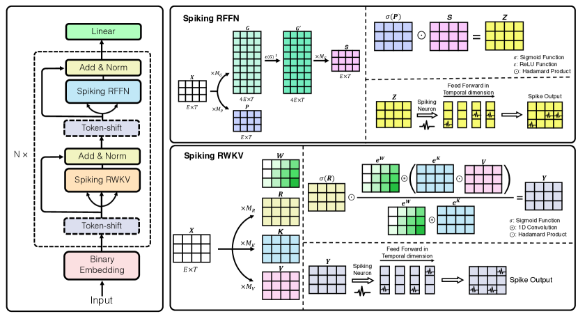
Figure 1: Model Architecture. The left portion displays the overall structure, while the bottom right and top right illustrations demonstrate the Spiking RWKV and Spiking RFFN architectures, respectively. The Spiking RWKV serves as a token-mixer and the Spiking RFFN functions as a channel mixer. These components are arranged in a loop with residual connections in a manner akin to a Transformer architecture.

3.1 Model Architecture

The high-level architecture of SpikeGPT is shown in Fig. 1. We adopt the Transformer paradigm of alternating token-mixer and channel-mixer layers. In SpikeGPT, the token-mixer is a Spiking RWKV layer, which replaces the self-attention mechanism with an RNN-like structure that preserves parallelization. The ’W’ in RWKV is a weight vector with learnable, time-varying dynamics (Fig. 1). The use of dynamical weights contributes to the ability of sequential models to retain long-range memory comparable to self-attention. The channel-mixer is a Spiking RFFN layer, which is stacked in a loop with residual connections. The following sections formalize the various model components.

3.2 Binary Embedding

To maintain consistency with the binary activations of SNNs, we propose a binary embedding step to convert the continuous outputs of the embedding layer into binary spikes. The conversion is performed using a Heaviside function for feed-forward propagation, which maps the continuous values to binary spikes. As this is a non-differentiable function, the arctangent function (a Sigmoid-like shape) is applied as a ‘surrogate gradient’ for backward propagation to provide a biased gradient estimator [11; 26], which can be represented as:

$$\sigma^{\prime}(x)=\frac{\alpha}{2(1+(\frac{\pi}{2}\alpha x)^{2})}$$ (1)

This allows us to convert continuous embedding values into spikes using non-differentiable functions, while still being able to perform backpropagation and update the weights of the embedding layer [26].

3.3 Token Shift

Given an input $X$, we perform a token shift operation on it as follows:

$$X_{s}=\text{ZeroPad}_{[0,0,-1,1]}(X)$$ (2)

$$W_{\rm shift}=\left[(\frac{i}{E})^{n/N}\right],i=1,\cdots,E$$

$$\mathcal{X}=W_{\rm shift}\odot X+(1-W_{\rm shift})\odot X_{s}$$

where ZeroPad denotes the zero padding operation, $W_{\rm shift}$ represents a learnable shift mask, $E$ is the embedding size of each token, $n$ is the current block, and $N$ is the total number of blocks.

The token shift operator combines information from the global context with information of the original token to provide the token with better contextual information. This strengthens the connection between the token and its neighboring tokens, making it easier for the model to learn the token combinations that have appeared before. This is similar to the induction head [27]. To some extent, token shift is a lightweight and inexpensive alternative to the attention mechanism.

3.4 Spiking RWKV

In this section, we first present the vanilla RWKV  [28] model and its main components. Next, we illustrate how positional weight decay enables the model to capture long-range dependencies and how the RWKV model can be parallelized. Then, we describe how spiking neurons can be integrated into RWKV with a recurrent structure.

Recall Self-Attention. The self-attention operation lies at the heart of Transformers. In Transformers, self-attention takes an input sequence $X$, and applies a scaled dot product attention. Formally, self-attention is defined as:

$$f(X)=\sigma\left(\frac{Q(K)^{T}}{\sqrt{d_{k}}}\right)V,\text{s.t.}~{}Q=XM_{Q},K=XM_{K},V=XM_{V}$$ (3)

where $M_{Q}\in\mathbb{R}^{d\times d_{k}}$, $M_{K}\in\mathbb{R}^{d\times d_{k}}$, $M_{V}\in\mathbb{R}^{d\times d_{v}}$ are linear transformations, and $\sigma$ is the non-linearity function by default set as the softmax (applied to each row of a matrix). $d_{k}$, $d_{v}$ are dimensions for key and value, respectively. Self-attention enables the model to learn the dependencies between any two tokens in a sequence.

Similarity to Multi-Headed Self-Attention. Distinct from the method of calculating the matching degree between tokens by the self-attention mechanism, RWKV decomposes the calculation of matching degree into: $\alpha_{ij}=\sigma(R_{i})\odot\text{exp}({W}_{T-i+1})\odot\text{exp}(K_{j})$, where $\alpha_{ij}\in\mathbb{R}^{E}$ is a vector. Each element in $\alpha_{ij}$, that is $\alpha_{ijk}$, represents the matching degree at the k-th position of the embedding of the i-th and j-th tokens. In other words, it can be seen as a multi-headed RWKV with $E$ heads, each of which has a hidden size=$1$, which is similar to the multi-headed self-attention (MHA) mechanism.

Vanilla RWKV. Inspired by the Attention Free Transformer [29], RWKV acts as a replacement for self-attention. It reduces computational complexity by swapping matrix-matrix multiplication with a convolution that sweeps along the time dimension. We subsequently modify this step to instead operate recurrently on input data. This modification enables compatibility with recurrent SNNs, thus making it more manageable to run on limited resources.

Given an input token-shifted embedding vector $\mathcal{X}$, similar to self-attention, RWKV first applies a linear transform $R=\mathcal{X}M_{R}$, $K=\mathcal{X}M_{K}$, $V=\mathcal{X}M_{V}$. $\mathcal{X}$ is a time-varying embedding (varying over the sequence), and so $R,K,V$ are also time-varying. Fig. 1 depicts the sequence unrolled into a set of 2-D matrices.

$M_{R}$, $M_{K}$ and $M_{V}$ consist of learnable parameters, where $K$ and $V$ can be likened to the key and value matrices of self-attention. $R$ is referred to as the receptance matrix, where each element indicates the acceptance of past information.

Next, the following operation is applied:

$$Y_{t}=\sigma(R_{t})\odot\frac{\sum_{i=1}^{t}{\text{exp}({W}_{(T+i-t)})\odot\text{exp}(K_{i})\odot V_{i}}}{\sum_{i=1}^{t}{\text{exp}({W}_{(T+i-t)})\odot\text{exp}(K_{i})}}$$ (4)

where $\odot$ is the element-wise product, $T$ is the sequence length, $\sigma$ is the non-linearity applied to $R$ with the default being Sigmoid; ${W}\in\mathbb{R}^{T\times E}$ is the positional weight decay matrix (represented as a vector unrolled over time in Fig. 1). ${W}$ encodes the sequential importance of a given word on subsequent words. It is not directly learnable, but it varies over time with learnable dynamics. Long-range dependence can be captured when the dynamics are learnt to decay slowly.

Intuitively, as time $t$ increases, the vector $Y_{t}$ is dependent on a longer history, represented by the summation of an increasing number of terms. For the target position $t$, RWKV performs a weighted summation in the positional interval of $[1,t]$, and takes the Hadamard product of the weighted result with the receptance $\sigma(R_{t})$. By taking the Sigmoid of $R_{t}$, the receptance acts as a ‘forget gate’ by eliminating unnecessary historical information.

Positional Weight Decay. The positional weight decay factor $W$ is a function of both learnable parameters and pre-calculated matrices formalized below. As it is not directly learnable, we empirically determined that it is important to properly parameterize the positional bias ${W}$. In general, for a given word, the elements of ${W}$ decay over the sequence with a constant rate. When this rule of thumb does not hold, this likely means the model is embedding long-range dependencies across a sequence. In general, ${W}$ should satisfy the characteristic that the weight decays with the change of position. The positional weight bias matrix $W$ is determined by three matrices, $W_{d}$, $W_{c}$ and $W_{f}$, and is calculated as below:

$$W_{d} =\ln(W_{s}),W_{s}\in\mathbb{R}^{E\times 1}$$ (5)

$$W_{c} =\begin{bmatrix}(-T+2)&(-T+3)&(-T+4)&\cdots&-1&0\end{bmatrix}\in\mathbb{R}^{1\times(T-1)}$$ (6)

$$W_{f} =\begin{bmatrix}\ln(p_{k})\ \ln(p_{k})\ \cdots\ \ln(p_{k})\end{bmatrix}\in\mathbb{R}^{E\times 1}$$ (7)

where $W_{s}$ is a pre-calculated matrix dependent on the layer and size of $E$, the vector $W_{d}$ contains the decay factors for each time-step, $W_{c}$ is an indicator of time-step, and $W_{f}$ is the initial decay factor to avoid the constant decay phenomenon of RNNs. $W_{d}$ and $W_{f}$ are both learnable, and $W_{c}$ is a static, pre-calculated matrix based on training time-step. $p_{k}$ is a hyperparameter, which is set to $0.3$ in this paper. These matrices combined the $W$ as below:

$$W=\text{exp}(concat(W_{d}\times\text{exp}(W_{c}),W_{f})),W\in\mathbb{R}^{E\times T}$$ (8)

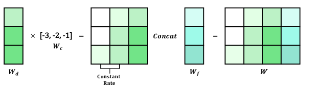
Figure 2: Construction of the weight decay matrix. $W_{d}$ is the decay factor vector and uses $W_{c}$ to obtain the actual decay value at each time-step. $W_{f}$ is the decay factor of the initial time-step, and is concatenated with the previous decay factor to derive the final weight decay $W$. The weight decay $W$ is represented as a vector unrolled over time into a matrix.

where $concat$ denotes the concatenation of two tensors in the temporal dimension, and the operator ‘$\times$’ is the outer-product of two vectors. To illustrate the construction of the weight decay factor more clearly, we provide a schematic diagram in Fig. 2.

Parallelize RWKV using 1-D Convolution. Eq. 4 only calculates the weighted summation across target positions $t$. On the basis of Eq. 4, the values of all target positions can be represented as a 1-D convolution:

$$Y=\sigma(R)\odot\frac{\text{exp}({W})\otimes(\text{LeftPad}(\text{exp}(K)\odot V))}{\text{exp}({W})\otimes\text{LeftPad}(\text{exp}(K))}$$ (9)

where $\otimes$ denotes the 1-D convolution operation, LeftPad applies zero-padding to all columns preceding the $T-1^{th}$ position.

Consider ${W}$ to be a large convolutional kernel, performing a convolution with the matrix $\text{exp}(K)$ (or $\text{exp}(K)\odot V$). The computational complexity of the complete convolution is $\mathcal{O}(ET^{2})$ (assuming the number of filters matches the sequence length, and $E$ is the embedding size). This can be further optimized by adopting the Fast Fourier Transform ($FFT$) to reduce the time complexity of the whole convolution operation to $\mathcal{O}(ET\text{log}T)$.

Integration with Spiking Neurons. The behavior of individual spiking neurons in an SNN is often described using differential equations, which cannot be solved analytically in closed-form expressions. In the context of recurrent networks, these equations must be solved numerically, which typically requires iterative methods that calculate the system’s behavior step-by-step over time. Fortunately, from Eq. 4, we are able to derive a recurrent form of RWKV, which is perfectly compatible with recurrent SNNs. The serial recursive form of RWKV is expressed as follows:

$$Y[t+1]=\sigma({R}X[t])\cdot\frac{\exp({K}X[\mathrm{t}])\cdot({V}X[\mathrm{t}])+\exp({W})\cdot A[\mathrm{t}]}{\exp({K}X[\mathrm{t}])+\exp({W})\cdot B[\mathrm{t}]}$$ (10)

where $t$ represents the time step index, and variables $R,W,K,V$ are also derived from the linear transformation $R=\mathcal{X}M_{R}$, $K=\mathcal{X}M_{K}$, $V=\mathcal{X}M_{V}$. The hidden states $A$ and $B$ are represented by

$$A[t]=\exp({K}X[\mathrm{t-1}])\cdot({V}X[\mathrm{t-1}])+\exp({W})\cdot A[\mathrm{t-1}]$$ (11)

and

$$B[t]=\exp({K}X[\mathrm{t-1}])+\exp({W})\cdot B[\mathrm{t-1}]$$ (12)

Finally, we integrate the spiking neuron model into the Spiking RWKV module. As RWKV has been serialized, not only does the memory complexity during training decrease from $\mathcal{O}(ETlogT)$ (as a convolution) to $\mathcal{O}(ET)$ (as an RNN), but the output of RWKV can be sequentially passed directly to spiking neurons without having to unsqueeze dimensions for the forward-pass. This is in stark contrast to prior SNN-based Transformers which combine matrix-matrix multiplications with recurrence, leading to cubically scaling computational complexity with sequence length, without enhancing the network’s ability to learn sequential information. Consequently, we achieve a more streamlined approach in our feed-forward process, allowing us to effectively process data in a streaming manner.

We employ the Leaky Integrate-and-Fire (LIF) neuron as the default spiking neuron of our model, a widely used model for SNNs often trained via error backpropagation [5]. The LIF dynamics are represented as follows:

$$\left\{\begin{array}[]{l}U[t]={H[t]}+\beta({Y[t]}-({H[t-1]}-{U}_{\text{reset}}))\\ {S[t]}={\Theta}({U[t]}-{U}_{\text{threshold}})\\ {H[t]}={U[t]}\cdot(1-{S[t]})\\ \end{array}\right.$$ (13)

where $\beta$ is a decay factor, $U$ is the membrane potential (or hidden state) of the neuron, $S$ is the spiking tensor with binarized elements, $Y$ denotes the output of the previous series RWKV block (see Eq. 10), ${\Theta(\cdot)}$ denotes the Heaviside function, and $H$ represents the reset process after spike emission. We set $U_{\rm threshold}=1$, $U_{\rm reset}=0$ and $\beta=0.5$ as done in Refs. [30; 31; 32].

To overcome the non-differentiable problem during back-propagation caused by the Heaviside step function ${\Theta(\cdot)}$, we employ the surrogate gradient approach. As with the binary embedding in Sec. 3.2, we utilize the arctangent surrogate function (Eq. 21) during the backward pass.

3.5 Spiking Receptance Feed-Forward Networks (SRFFN)

Each block in our model contains a fully connected feed-forward network with a gating mechanism (SRFFN), which is applied to normalized and token-shifted outputs of each spiking-RWKV module. This SRFFN module consists of three linear transformations with $ReLU^{2}$ activations as follows:

$$Y^{\prime}[t]=\sigma(M_{P}X[t])\odot M_{S}(ReLU^{2}(M_{G}X[t]))$$ (14)

where $Y^{\prime}[t]$ denotes the output of SRFFN at time-step $t$ which is then passed to the spiking neuron (Eq. 13). $\{M_{P},M_{G},M_{S}\}\in\mathbb{R}^{E\times H}$ are learnable parameters of the linear transformations. SRFFN is a variant of the Gated Linear Unit (GLU) [33], which can control the degree of information flowing into the model by $\sigma(M_{P}X[t])$. In order to maintain consistency between SRFFN and GEGLU parameters [34], we set the size of $H$ from the SRFFN to $4E$.

3.6 Training & Inference

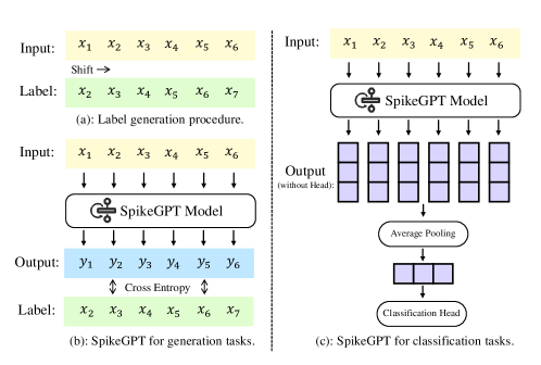
Figure 3: Training SpikeGPT for NLG and NLU tasks.

Our training procedure consists of two stages. The first stage is pre-training on a large-scale corpus to build a high-capacity language model, and the next stage is specific fine-tuning to perform downstream tasks, such as natural language generation (NLG) and natural language understanding (NLU).

We adopt a decoder-only pre-training paradigm similar to GPT to train the model. Specifically, our model utilizes Spiking RWKV and SRFFN modules to process the input token sequence and generate an output distribution for each target token.

Formally, given a token sequence $\mathcal{C}=\{c_{1},c_{2},\cdots,c_{n}\}$, we use the standard language modeling objective to maximize the following likelihood:

$$\mathcal{P}(c_{t})=\text{softmax}(Y^{\prime}[t]W_{e}^{T})$$ (15)

$$\mathcal{L}_{p}=\sum_{i=1}^{T}{log\mathcal{P}(c_{i}|c_{1},c_{2},\cdots,c_{i-1};\Theta)}$$ (16)

where $W_{e}^{T}$ is the token embedding matrix, and $\Theta$ is the set of all model parameters.

After pre-training the model using the loss in Eq. 16, model parameters are fine-tuned to adapt to different downstream tasks in natural language generation and understanding. For natural language generation tasks, suppose a new dataset $\mathcal{D}_{G}$, where each instance consists of a sequence of input tokens. Thanks to the consistency between the pre-training process and the NLG task, the fine-tuning procedure could directly reuse the pre-training pipeline (Eq. 15 and Eq. 16), which maximizes the likelihood of the target token based on the previous information of the target position.

As for natural language comprehension tasks, such as sentiment classification, it is worth noting that there is a certain degree of mismatch between pre-training and the downstream task. Hence, during the fine-tuning process, we made several modifications to the top-level of the pre-trained SpikeGPT model to adapt to NLU tasks, as shown in Fig. 3. Specifically, given a new dataset for the downstream task $\mathcal{D}_{U}$, where each instance consists of a token sequence $\mathcal{C}_{i}$ and label $l_{i}$, the following objective is maximized:

$$\mathcal{L}_{NLU}=\sum_{(\mathcal{C}_{i},l_{i})}{l_{i}*log{P}(\mathcal{C}_{i})}$$ (17)

where $\mathcal{P}(\mathcal{C}_{i})$ is defined as:

$$\mathcal{P}(\mathcal{C}_{i})=\text{softmax}(\hat{Y}W_{m}^{T})\\$$ (18)

$W_{m}^{T}$ includes the learnable parameters of the MLP module in the top layer, and $\hat{Y}$ is generated by passing the input token sequence $\mathcal{C}_{i}$ through our model and then averaging pooling the embedding of each target, which is formalized as:

$$\hat{Y}=\text{AvgPooling}(Y^{\prime}[1],Y^{\prime}[2],\cdots,Y^{\prime}[T])$$ (19)

In the inference phase, we directly give a prompt for the NLG task, and let the model continue and calculate bits-per-character (BPC) and perplexity (PPL) as an evaluation metric. For the NLU task, we pass the inputs through our model to obtain the embedding over target positions, and then conduct mean pooling operation to all embedded tokens to predict the label of each instance.

3.7 Complexity Analysis

For the Spiking RWKV module, adopting the RNN training paradigm means that given an input $X$ with a length of $N$ and an embedding size of $E$, Eq. 10 is used to generate each target location $t$. Hence, from Eq. 10, given a target $Y[t]$, for a single Spiking RWKV module, only 1) a series of non-linear transformations (${K}X[\mathrm{t}]$, ${V}X[\mathrm{t}]$, ${R}X[\mathrm{t}]$) are applied to input $X$, which are essentially vector-matrix multiplications. Thus, its time complexity is $\mathcal{O}(E)$, where only the hidden states need to be stored, leading to an identical spatial complexity that scales with $\mathcal{O}(E)$; 2) Past information decay ($\exp({W})\cdot A[\mathrm{t}]$) is essentially a Hadamard product between one-dimensional vectors, so its time and spatial complexity are both $\mathcal{O}(E)$. For the full architecture, there are a total of $N$ target positions with an overall time complexity of $\mathcal{O}(N\cdot E)$, and Spiking RWKV can recursively utilize hidden states, resulting in an overall spatial complexity of $\mathcal{O}(E)$.

4 Experiments

We evaluated SpikeGPT on two major language-related tasks: Natural Language Generation (NLG) and Natural Language Understanding (NLU). For NLG, we evaluated the text generation performance of SpikeGPT on three classic text generation datasets: Enwik8 [35], WikiText-2 [36], and WikiText-103 [36]. These datasets are widely used to measure a model’s ability to perform compression and for benchmarking. For NLU, we evaluated the performance of SpikeGPT on four classic text classification datasets: MR [37], SST-5 [38], SST-2 [38], and Subj [39]. These datasets cover sentiment analysis and subjective/objective classification. Our implementation is based on PyTorch [40] and SpikingJelly [41].

4.1 Datasets

We conducted experiments on two major types of tasks, Natural Language Generation (NLG) and Natural Language Understanding (NLU).
For NLG tasks, we chose the following 3 classic text classification datasets to evaluate the text generation performance of SpikeGPT: Enwik8 [35], WikiText-2 [36] and WikiText-103 [36].

• Enwik8. The Enwik8 dataset is a subset of the English Wikipedia XML dump from March 2006. It contains the first 100 million bytes of the dump and is typically used to measure a model’s ability to compress data. The dataset is based on the Hutter Prize, a competition for lossless compression of human knowledge. We split the tokens into three subsets: 90% for training, 5% for validation, and 5% for testing.

• WikiText-2. WikiText-2 is a natural language dataset comprising a collection of 2 million tokens derived from Wikipedia articles. This dataset is commonly utilized for benchmarking various natural language processing models.

• WikiText-103. The Wikitext-103 dataset is a large collection of text extracted from Wikipedia articles that are verified as Good or Featured. It contains over 100 million tokens and covers a wide range of topics and domains. The dataset is suitable for language modeling tasks that require long-term dependencies and rich vocabulary. The Wikitext-103 dataset is a larger and more diverse version of the Wikitext-2 dataset.

For NLU tasks, we chose the following 4 classic text classification datasets to evaluate the performance of our proposed SpikeGPT: MR [37], SST-5 [38], SST-2 [38], Subj. [39]

• MR [37]. It consists of movie review files, labeled based on their overall sentiment polarity (positive or negative) or subjective rating.

• SST-5. The Stanford Sentiment Tree Library 5 includes 11855 sentences extracted from movie reviews for sentiment classification [38]. There are 5 different categories (very negative, negative, neutral, positive, and very positive)

• SST-2 [38]. It is a binary version of SST-5, with only two classes (positive and negative).

• Subj [39]. Classify sentences in the dataset as subjective or objective.

The sample sizes and text lengths of these datasets vary. If there is no standard training test segmentation, we will follow [19] and randomly select 10% of the samples from the entire dataset as the test set.

4.2 Baselines

To verify the effectiveness on NLG and NLU tasks of our proposed SpikeGPT, we compare it with the following representative baselines:

For NLG, we list the baselines that we have selected as follows:

• Stacked LSTM. A model architecture that stacks multiple LSTM modules together.

• SHA-LSTM [42]. An LSTM model that follows by a single attention head layer.

• Transformer [18]. Transformer is a state-of-the-art neural network architecture, leveraging self-attention mechanisms to capture global dependencies of sequential data.

• Reformer [43]. Reformer is an extensible variant of the Transformer model. By introducing the invertible sheaf and using the local sensitive hash mechanism, it solves the problem of low memory and computing efficiency of the traditional Transformer, and realizes efficient processing of long sequences.

• Synthesizer [44]. Synthesizer is also a variant of Transformer, which is a model that learns to synthesize attention weights without token-token interaction.

• Linear Transformer [45]. Linear Transformer is a lightweight variant of Transformer that uses linear transformation layers to construct a self attention mechanism.

• Performer [46]. A variant of Transformer that does not depend on sparsity or low-rankness assumptions and could use linear complexity to accurately estimate attention weights.

• GPT-2 [47]. GPT-2 is a transformer-based language model that specifically functions as a decoder. It is an extensively trained, large-scale generative model using the autoregressive paradigm. To ensure compatibility with the parameter sizes of SpikeGPT, we selected GPT-2 medium and GPT-2 small as suitable alternatives.

For NLU, the baselines we have selected are as follows:

• LSTM [48]. LSTM model is a type of recurrent neural network with the ability to capture and utilize long-term dependencies in input sequences.

• TextCNN [49]. TextCNN is a convolutional neural network architecture specifically designed for text classification tasks, leveraging convolutional layers to capture local patterns and features in textual data.

• TextSCNN [19]. A variant of TextCNN model that combines spiking neural networks.

• BERT [50]. BERT is a bidirectional language model based on the Transformer Encoder-only architecture and an auto-encoding training paradigm.

4.3 Experiment Settings

We test two variants of the 45 million parameter model; one where $T=1,024$ and another where $T=3,072$. We used the Enwik8 dataset to conduct both training and testing in 45M scale, and our most extensive model with 216 million parameters was trained using the OpenWebText2 [51] corpus for pre-training. Zero-shot text samples of this experiment can be found in Appendix LABEL:app:gen. In our 45M model, we employ a character-level tokenizer, as has been done in previous works [29]. To evaluate the performance of our model, we calculate its BPC metrics. To mitigate the issue of overfitting, we incorporate dropout after the output of each SRFFN block and set the dropout ratio to 0.03. In our 216M model with pre-training, we employ the Byte Pair Encoding (BPE) tokenizer and share the same hyper-parameters as GPT-NeoX [52]. Due to the availability of sufficient data for pre-training, we do not incorporate dropout as we did in our 45M model and remove the binary embedding but use the first layer neurons for encoding. To facilitate better convergence, we utilize a warmup technique during the first 500 training steps. For both the 45M and 216M models, we use the Adam optimizer, and set the learning rate to $6\times 10^{-4}$ and $6\times 10^{-4}$, respectively. All experiments were conducted on four NVIDIA V100 graphic cards. For the models of 45M and 216M, we trained them for 12 and 48 hours respectively.

4.4 Results on Natural Language Generating Tasks

A summary of results are provided in Tabs. 1 and 2. This includes the BPC and PPL achieved on NLG tasks using SpikeGPT trained on Enwik8, WikiText-103, and WikiText-2 compared to several baselines, including 45M and 216M parameter variants.

Table 1: Enwik8 results. Measured in Bits Per Character (BPC): the lower the better. Baseline comparisons are made with Reformer [43], Synthesizer [44] (the best performing dense version), Linear Transformer [53], Performer [46], Stacked LSTM [54] and SHA-LSTM [42]. $L,d$ and $N$ denote the number of blocks (network depth), dimension of features, and sequence length, respectively. Both Linear Transformer and Performer are implemented with customized CUDA kernels (github.com/idiap/fast-transformers), and all other models are implemented in native Pytorch.

Method	Spiking	$L$	$d$	$N$	Train BPC	Test BPC	SynOps
Transformer	✗	12	512	1024	0.977	1.137	$9.6\times 10^{10}$
Transformer	✗	24	256	1024	1.039	1.130	-
Reformer	✗	12	512	1024	1.040	1.195	-
Synthesizer	✗	12	512	1024	0.994	1.298	-
Linear Transformer	✗	12	512	1024	0.981	1.207
Performer	✗	12	512	1024	1.002	1.199	-
Stacked LSTM	✗	7	-	-	1.420	1.670	-
SHA-LSTM (no attention)	✗	4	1024	1024	-	1.330	-
SpikeGPT 45M	✓	12	512	1024	1.113	1.283	$\boldsymbol{4.35\times 10^{9}}$
SpikeGPT 45M	✓	12	512	3072	0.903	1.262	$\boldsymbol{1.30\times 10^{10}}$

Firstly, we report two variants of SpikeGPT and some baseline methods for training and testing BPC on dataset Enwik8 dataset. As shown in Tab. 1, the generative performance of SpikeGPT has far surpassed that of models with an LSTM backbone, and can approach or even surpass some simplified variants of the Transformer, such as Linear Transformer and Synthesizer. However, it should be pointed out that there is still a certain gap between SpikeGPT and the vanilla Transformer. While increasing the size of $N$ significantly reduces the training BPC of SpikeGPT, its test BPC has not changed significantly, indicating that SpikeGPT is potentially suffering from over-fitting.

Secondly, the energy efficiency of SNNs is largely derived from sparse memory access patterns arising from activation sparsity. ‘Synaptic Operations’ (SynOps) is a common metric used to estimate SNN efficiency by counting the number of non-zero multiply-accumulate operations. Due to the activation sparsity of SpikeGPT, our proposed models exhibit significantly lower SynOps compared to the vanilla Transformer. Specifically, our models achieve an increase of over 20$\times$ in computational efficiency compared to the vanilla Transformer.

Thirdly, we also compared the Perplexity of SpikeGPT and GPT-2 based on WikiText-2 and WikiText-103 datasets on text generation tasks. The results are shown in Tab. 2. In the interest of fairly comparing models of similar scales, we selected GPT-2 small and GPT-2 medium [47] with parameter sizes similar to those of the fine-tuned 216M SpikeGPT. We found that after fine-tuning, the performance of SpikeGPT on WikiText-2 has surpassed that of GPT-2 series. Unfortunately, the performance of SpikeGPT on the larger WikiText-103 dataset has fallen behind the GPT-2 series models, which indicates that SpikeGPT requires more scientific training strategies to learn larger scale corpus knowledge.

Table 2: Results on WikiText-2 and WikiText-103 measured in token-level perplexity. Lower values indicate better performance. We report the perplexity when the lowest value was achieved on the validation datasets. Note that for WikiText-2, we use both the WikiText-103 and WikiText-2 training sets to extend the training corpus.

      Method       Parameters       WikiText-103       WikiText-2       Val.       Test.       Val.       Test.       GPT-2 Small  [47]       124M       -       29.41       -       37.50       GPT-2 Medium  [47]       345M       -       26.37       -       22.76       SpikeGPT With Pre-training       216M       39.92       39.75       19.17       18.01

4.5 Results on Natural Language Understanding Tasks

For NLU tasks, we utilize SpikeGPT as a dynamic embedding generator that constructs embeddings based on context. We compare SpikeGPT with text classification algorithms of similar scales, including LSTM [48], TextCNN [49], BERT [50], and the latest SNN-based text classification algorithm TextSCNN [19]. The accuracy on four datasets is shown in Tab. 3. The fine-tuned 216M SpikeGPT achieves the second-highest performance among the models, only surpassed by BERT. BERT is a bidirectional Transformer encoder that uses masked training to obtain a high-quality text embedding. However, unlike SpikeGPT, BERT does not have the capability to generate text directly. Our 45M model without any fine-tune also achieves competitive results compared to the baseline models, indicating the enormous potential of SpikeGPT in NLU tasks. We also analyze the complexity of each method and show that SpikeGPT can achieve linear complexity by using spiking neurons and a recurrent structure. Unlike TextSCNN, our model does not require an additional temporal dimension for processing, as it uses the sequence dimension as the basis for spiking neuron feed-forward.

Table 3: Results of NLU tasks on four text classification datasets using both SNN and ANN methods. Measured in classification accuracy: the higher the better. In the ’complexity per layer’ column, we compute the complexity of each method using the following notation: $N$ is sequence length, $E$ is the embedding dimension, $K$ is the convolution kernel size, and $T$ is the additional temporal dimension for feed-forward processing. Our model combines recurrent and spiking features and does not need an extra temporal dimension for feed-forward processing, as it exploits the inherent temporal dimension in the language model.

Method Spiking Recurrent Complexity per layer SST-2 SST-5 MR Subj. TextCNN [49]^EMNLP ✗ ✗ $\mathcal{O}(K\cdot N\cdot E^{2})$ 81.93 44.29 75.02 92.20 TextSCNN-Direct Training [19]^ICLR-2023 ✓ ✗ $\mathcal{O}(T\cdot K\cdot N\cdot E^{2})$ 75.73 23.08 51.55 53.30 TextSCNN-ANN2SNN+Fine-tune [19]^ICLR-2023 ✓ ✗ $\mathcal{O}(T\cdot K\cdot N\cdot E^{2})$ 80.91 41.63 75.45 90.60 LSTM [55] ✗ ✓ $\mathcal{O}(N\cdot E^{2})$ 84.92 46.43 81.60 - BERT [50] ✗ ✗ $\mathcal{O}(N^{2}\cdot E)$ 91.73 53.21 86.72 - SpikeGPT 45M ✓ ✓ $\mathcal{O}(N\cdot E)$ 80.39 37.69 69.23 88.45 SpikeGPT 216M ✓ ✓ $\mathcal{O}(N\cdot E)$ 82.45 38.91 68.11 89.10 SpikeGPT 216M With Pre-training ✓ ✓ $\boldsymbol{\mathcal{O}(N\cdot E)}$ 88.76 51.27 85.63 95.30

4.6 Discussions

Visualization of Spike and Membrane Potential

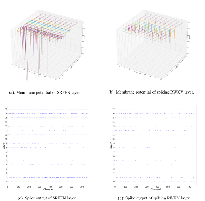
Figure 4: Visualization of spike and membrane potential of neurons. Figures (a) and (b) depict the membrane potential of the SRFFN layer, while Figures (c) and (d) display the spike patterns observed in the SRFFN layer, where each dot represents a spike event.

To gain a more comprehensive understanding of SpikeGPT, we conducted visualizations of the spike and membrane potential patterns in the Spiking RWKV layer and Spiking Receptance Feed-Forward Networks (SRFFN) layers (Fig. 4). These visualizations clearly reveal distinct differences between the Spiking RWKV and SRFFN layers, indicating diverse information representation patterns. Notably, the SRFFN layer exhibits a higher firing rate, suggesting that it may retain more information similar to Transformer FFN layers [56]. It is worth noting that in various studies, outliers in Transformer-based language models have been shown to significantly impact performance, making them a crucial concern in the quantification of large language models [57]. Therefore, understanding and addressing the implications of outliers in SpikeGPT are of utmost importance, particularly in the context of optimizing its overall performance and reliability. However, due to the binary nature of SNNs, these outliers cannot be expressed in activation values as in ANNs. Nevertheless, a notable observation is the presence of prominent outliers in the membrane potential of individual neurons, many of which are negative. This finding suggests that SpikeGPT employs a different approach to accommodate and preserve outliers.

RWKV Binariziation with LIF neurons

We conducted an exploration by utilizing the Heaviside function to directly binarize the RWKV layer, instead of employing the LIF neuron. Specifically, we utilize the Heaviside function for the feed-forward process, represented as follows:

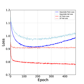
Figure 5: Training and Validation Loss of SpikeGPT Variants during Training.

$$H(x)=\begin{cases}0,&\text{if }x<0\\ 1,&\text{if }x\geq 0\end{cases}$$ (20)

To address the non-differentiable nature of the Heaviside function during the backward pass, we employ the arctangent function, given by:

$$\sigma^{\prime}(x)=\frac{\alpha}{2(1+(\frac{\pi}{2}\alpha x)^{2})}$$ (21)

The training and validation losses are shown in Fig. 5. Both approaches were trained for 500 epochs using identical hyperparameters. It is evident that employing the recurrent LIF neuron leads to superior performance in terms of lower loss values across both the training and validation datasets. We attribute this improvement to the role played by the LIF neuron as a token-mixer. This enables the FFN layer to function effectively as a token-mixer, thereby enhancing token mixing performance and subsequently resulting in overall improved model performance.

5 Conclusion

Our results demonstrate that event-driven spiking activations are not only capable of language generation, but they can do so with fewer high-cost operations. We develop techniques that promote lightweight models for the NLP community, and make large-scale models for the neuromorphic and SNN community more effective. We demonstrate how large SNNs can be trained in a way that harnesses advances in transformers and our own serialized version of the attention mechanisms. An open-source repository for training SpikeGPT, along with a set of fine-tuned models will be made available online upon conclusion of the anonymous peer review process. These have been included in the supplementary materials in the meantime. We expect this research can open new directions for large-scale SNNs.

References

- [1] Tom Brown, Benjamin Mann, Nick Ryder, Melanie Subbiah, Jared D Kaplan, Prafulla Dhariwal, Arvind Neelakantan, Pranav Shyam, Girish Sastry, Amanda Askell, et al. Language models are few-shot learners. Advances in Neural Information Processing Systems (NeurIPS), 33:1877–1901, 2020.
- [2] Payal Dhar. The carbon impact of artificial intelligence. Nature Machine Intelligence, 2:423–5, 2020.
- [3] Lasse F Wolff Anthony, Benjamin Kanding, and Raghavendra Selvan. Carbontracker: Tracking and predicting the carbon footprint of training deep learning models. arXiv preprint arXiv:2007.03051, 2020.
- [4] OpenAI. ChatGPT: Optimizing language models for dialogue. https://openai.com/blog/chatgpt/. Accessed: 2023-02-18.
- [5] Wolfgang Maass. Networks of spiking neurons: the third generation of neural network models. Neural Networks, 10(9):1659–1671, 1997.
- [6] Mike Davies, Narayan Srinivasa, Tsung-Han Lin, Gautham Chinya, Yongqiang Cao, Sri Harsha Choday, Georgios Dimou, Prasad Joshi, Nabil Imam, Shweta Jain, et al. Loihi: A neuromorphic manycore processor with on-chip learning. IEEE Micro, 38(1):82–99, 2018.
- [7] Paul A Merolla, John V Arthur, Rodrigo Alvarez-Icaza, Andrew S Cassidy, Jun Sawada, Filipp Akopyan, Bryan L Jackson, Nabil Imam, Chen Guo, Yutaka Nakamura, et al. A million spiking-neuron integrated circuit with a scalable communication network and interface. Science, 345(6197):668–673, 2014.
- [8] Pao-Sheng Vincent Sun, Alexander Titterton, Anjlee Gopiani, Tim Santos, Arindam Basu, Wei D Lu, and Jason K Eshraghian. Intelligence processing units accelerate neuromorphic learning. arXiv preprint arXiv:2211.10725, 2022.
- [9] Kaushik Roy, Akhilesh Jaiswal, and Priyadarshini Panda. Towards spike-based machine intelligence with neuromorphic computing. Nature, 575(7784):607–617, 2019.
- [10] Michael Pfeiffer and Thomas Pfeil. Deep learning with spiking neurons: Opportunities and challenges. Frontiers in Neuroscience, 12:774, 2018.
- [11] Wei Fang, Zhaofei Yu, Yanqi Chen, Tiejun Huang, Timothée Masquelier, and Yonghong Tian. Deep residual learning in spiking neural networks. Advances in Neural Information Processing Systems (NeurIPS), 34:21056–21069, 2021.
- [12] Jason K Eshraghian, Max Ward, Emre Neftci, Xinxin Wang, Gregor Lenz, Girish Dwivedi, Mohammed Bennamoun, Doo Seok Jeong, and Wei D Lu. Training spiking neural networks using lessons from deep learning. arXiv preprint arXiv:2109.12894, 2021.
- [13] Yujie Wu, Lei Deng, Guoqi Li, Jun Zhu, and Luping Shi. Spatio-temporal backpropagation for training high-performance spiking neural networks. Frontiers in neuroscience, 12:331, 2018.
- [14] Youhui Zhang, Peng Qu, Yu Ji, Weihao Zhang, Guangrong Gao, Guanrui Wang, Sen Song, Guoqi Li, Wenguang Chen, Weimin Zheng, et al. A system hierarchy for brain-inspired computing. Nature, 586(7829):378–384, 2020.
- [15] Sami Barchid, José Mennesson, Jason Eshraghian, Chaabane Djéraba, and Mohammed Bennamoun. Spiking neural networks for frame-based and event-based single object localization. arXiv preprint arXiv:2206.06506, 2022.
- [16] Seijoon Kim, Seongsik Park, Byunggook Na, and Sungroh Yoon. Spiking-yolo: spiking neural network for energy-efficient object detection. In Proceedings of the AAAI conference on artificial intelligence (AAAI), volume 34, pages 11270–11277, 2020.
- [17] Loïc Cordone, Benoît Miramond, and Philippe Thierion. Object detection with spiking neural networks on automotive event data. In International Joint Conference on Neural Networks (IJCNN), pages 1–8, 2022.
- [18] Ashish Vaswani, Noam Shazeer, Niki Parmar, Jakob Uszkoreit, Llion Jones, Aidan N Gomez, Łukasz Kaiser, and Illia Polosukhin. Attention is all you need. In Advances in neural information processing systems (NeurIPS), pages 5998–6008, 2017.
- [19] Changze Lv, Jianhan Xu, and Xiaoqing Zheng. Spiking convolutional neural networks for text classification. In The Eleventh International Conference on Learning Representations (ICLR), 2023.
- [20] Jason K Eshraghian and Wei D Lu. The fine line between dead neurons and sparsity in binarized spiking neural networks. arXiv preprint arXiv:2201.11915, 2022.
- [21] Jason K Eshraghian, Xinxin Wang, and Wei D Lu. Memristor-based binarized spiking neural networks: Challenges and applications. IEEE Nanotechnology Magazine, 16(2):14–23, 2022.
- [22] Zhaokun Zhou, Yuesheng Zhu, Chao He, Yaowei Wang, Shuicheng YAN, Yonghong Tian, and Li Yuan. Spikformer: When spiking neural network meets transformer. In The Eleventh International Conference on Learning Representations (ICLR), 2023.
- [23] Rong Xiao, Yu Wan, Baosong Yang, Haibo Zhang, Huajin Tang, Derek F Wong, and Boxing Chen. Towards energy-preserving natural language understanding with spiking neural networks. IEEE/ACM Transactions on Audio, Speech, and Language Processing, 31:439–447, 2022.
- [24] Peter U Diehl, Guido Zarrella, Andrew Cassidy, Bruno U Pedroni, and Emre Neftci. Conversion of artificial recurrent neural networks to spiking neural networks for low-power neuromorphic hardware. In IEEE International Conference on Rebooting Computing (ICRC), pages 1–8, 2016.
- [25] Yudong Li, Yunlin Lei, and Xu Yang. Spikeformer: A novel architecture for training high-performance low-latency spiking neural network. arXiv preprint arXiv:2211.10686, 2022.
- [26] Emre O Neftci, Hesham Mostafa, and Friedemann Zenke. Surrogate gradient learning in spiking neural networks: Bringing the power of gradient-based optimization to spiking neural networks. IEEE Signal Processing Magazine, 36(6):51–63, 2019.
- [27] Catherine Olsson, Nelson Elhage, Neel Nanda, Nicholas Joseph, Nova DasSarma, Tom Henighan, Ben Mann, Amanda Askell, and et al. In-context learning and induction heads. CoRR, abs/2209.11895, 2022.
- [28] Bo PENG. RWKV-LM. https://github.com/BlinkDL/RWKV-LM, 8 2021.
- [29] Shuangfei Zhai, Walter Talbott, Nitish Srivastava, Chen Huang, Hanlin Goh, Ruixiang Zhang, and Josh Susskind. An attention free transformer. arXiv preprint arXiv:2105.14103, 2021.
- [30] Rui-Jie Zhu, Qihang Zhao, Tianjing Zhang, Haoyu Deng, Yule Duan, Malu Zhang, and Liang-Jian Deng. Tcja-snn: Temporal-channel joint attention for spiking neural networks. arXiv preprint arXiv:2206.10177, 2022.
- [31] Man Yao, Huanhuan Gao, Guangshe Zhao, Dingheng Wang, Yihan Lin, Zhaoxu Yang, and Guoqi Li. Temporal-wise attention spiking neural networks for event streams classification. In Proceedings of the IEEE/CVF International Conference on Computer Vision (ICCV), pages 10221–10230, 2021.
- [32] Man Yao, Guangshe Zhao, Hengyu Zhang, Yifan Hu, Lei Deng, Yonghong Tian, Bo Xu, and Guoqi Li. Attention spiking neural networks. IEEE Transactions on Pattern Analysis and Machine Intelligence, PP:1–18, 01 2023.
- [33] Yann N. Dauphin, Angela Fan, Michael Auli, and David Grangier. Language modeling with gated convolutional networks. In International Conference on Machine Learning (ICML), volume 70 of Proceedings of Machine Learning Research, pages 933–941, 2017.
- [34] Noam Shazeer. GLU variants improve transformer. CoRR, abs/2002.05202, 2020.
- [35] Matt Mahoney. Large text compression benchmark, 2011.
- [36] Stephen Merity, Caiming Xiong, James Bradbury, and Richard Socher. Pointer sentinel mixture models. In 5th International Conference on Learning Representations (ICLR), 2017.
- [37] Bo Pang and Lillian Lee. Seeing stars: Exploiting class relationships for sentiment categorization with respect to rating scales. arXiv preprint cs/0506075, 2005.
- [38] Richard Socher, Alex Perelygin, Jean Wu, Jason Chuang, Christopher D Manning, Andrew Y Ng, and Christopher Potts. Recursive deep models for semantic compositionality over a sentiment treebank. In Proceedings of the 2013 Conference on Empirical Methods in Natural Language Processing (EMNLP), pages 1631–1642, 2013.
- [39] Bo Pang and Lillian Lee. A sentimental education: Sentiment analysis using subjectivity summarization based on minimum cuts. arXiv preprint cs/0409058, 2004.
- [40] Adam Paszke, Sam Gross, Francisco Massa, Adam Lerer, James Bradbury, Gregory Chanan, Trevor Killeen, Zeming Lin, Natalia Gimelshein, Luca Antiga, et al. Pytorch: An imperative style, high-performance deep learning library. Advances in Neural Information Processing Systems (NeurIPS), 32, 2019.
- [41] Wei Fang, Yanqi Chen, Jianhao Ding, Ding Chen, Zhaofei Yu, Huihui Zhou, Timothée Masquelier, Yonghong Tian, and other contributors. Spikingjelly. https://github.com/fangwei123456/spikingjelly, 2020. Accessed: 2022-05-21.
- [42] Stephen Merity. Single headed attention RNN: stop thinking with your head. CoRR, abs/1911.11423, 2019.
- [43] Nikita Kitaev, Lukasz Kaiser, and Anselm Levskaya. Reformer: The efficient transformer. In 8th International Conference on Learning Representations (ICLR), 2020.
- [44] Y Tay, D Bahri, D Metzler, D Juan, Z Zhao, and C Zheng. Synthesizer: rethinking self-attention in transformer models. arXiv preprint arXiv:2005.00743, 2020.
- [45] Angelos Katharopoulos, Apoorv Vyas, Nikolaos Pappas, and François Fleuret. Transformers are rnns: Fast autoregressive transformers with linear attention. In Proceedings of the 37th International Conference on Machine Learning, ICML 2020, 13-18 July 2020, Virtual Event, volume 119 of Proceedings of Machine Learning Research, pages 5156–5165, 2020.
- [46] Krzysztof Choromanski, Valerii Likhosherstov, David Dohan, Xingyou Song, Andreea Gane, Tamas Sarlos, Peter Hawkins, Jared Davis, Afroz Mohiuddin, Lukasz Kaiser, et al. Rethinking attention with performers. arXiv preprint arXiv:2009.14794, 2020.
- [47] Alec Radford, Jeffrey Wu, Rewon Child, David Luan, Dario Amodei, Ilya Sutskever, et al. Language models are unsupervised multitask learners. OpenAI blog, 1(8):9, 2019.
- [48] Sepp Hochreiter and Jürgen Schmidhuber. Long short-term memory. Neural Computation, 9(8):1735–1780, 1997.
- [49] Yoon Kim. Convolutional neural networks for sentence classification. In Alessandro Moschitti, Bo Pang, and Walter Daelemans, editors, Proceedings of the 2014 Conference on Empirical Methods in Natural Language Processing (EMNLP), pages 1746–1751, 2014.
- [50] Jacob Devlin Ming-Wei Chang Kenton and Lee Kristina Toutanova. Bert: Pre-training of deep bidirectional transformers for language understanding. In Proceedings of NAACL-HLT (NAACL), pages 4171–4186, 2019.
- [51] Leo Gao, Stella Biderman, Sid Black, Laurence Golding, Travis Hoppe, Charles Foster, Jason Phang, Horace He, Anish Thite, Noa Nabeshima, et al. The pile: An 800gb dataset of diverse text for language modeling. arXiv preprint arXiv:2101.00027, 2020.
- [52] Sid Black, Stella Biderman, Eric Hallahan, Quentin Anthony, Leo Gao, Laurence Golding, Horace He, Connor Leahy, Kyle McDonell, Jason Phang, et al. Gpt-neox-20b: An open-source autoregressive language model. arXiv preprint arXiv:2204.06745, 2022.
- [53] A. Katharopoulos, A. Vyas, N. Pappas, and F. Fleuret. Transformers are rnns: Fast autoregressive transformers with linear attention. In International Conference on Machine Learning (ICML), 2020.
- [54] Alex Graves. Generating sequences with recurrent neural networks. arXiv preprint arXiv:1308.0850, 2013.
- [55] Kai Sheng Tai, Richard Socher, and Christopher D Manning. Improved semantic representations from tree-structured long short-term memory networks. arXiv preprint arXiv:1503.00075, 2015.
- [56] Mor Geva, Roei Schuster, Jonathan Berant, and Omer Levy. Transformer feed-forward layers are key-value memories. In Proceedings of the 2021 Conference on Empirical Methods in Natural Language Processing (EMNLP), pages 5484–5495, 2021.
- [57] Xiuying Wei, Yunchen Zhang, Xiangguo Zhang, Ruihao Gong, Shanghang Zhang, Qi Zhang, Fengwei Yu, and Xianglong Liu. Outlier suppression: Pushing the limit of low-bit transformer language models. In Advances in Neural Information Processing Systems (NeurIPS), 2022.