Multi-cell experiments for marginal treatment effect estimation of digital ads

Abstract

Randomized experiments with treatment and control groups are an important tool to measure the impacts of interventions. However, in experimental settings with one-sided noncompliance, extant empirical approaches may not produce the estimands a decision-maker needs to solve their problem of interest. For example, these experimental designs are common in digital advertising settings, but typical methods do not yield effects that inform the intensive margin—how many consumers should be reached or how much should be spent on a campaign. We propose a solution that combines a novel multi-cell experimental design with modern estimation techniques that enables decision-makers to recover enough information to solve problems with an intensive margin. Our design is straightforward to implement and does not require any additional budget to be carried out. We illustrate our approach through a series of simulations that are calibrated using an advertising experiment at Facebook, finding that our method outperforms standard techniques in generating better decisions.

Keywords: Marginal Treatment Effects, Field Experiments, Causal Inference, Digital Advertising, Advertising Measurement.

1 Introduction

Randomized experiments with treatment and control groups are considered a particularly reliable tool to measure the causal effects of interventions. However, decision-makers who conduct such experiments may be unsatisfied solely with measuring these causal effects; they need more information to inform specific decisions they have to make. Yet in a variety of settings, a decision-maker’s ability to experiment is limited because they cannot fully control treatment assignment.

In such cases, the most common experimental route involves randomizing eligibility to receive treatment. For example, firms want to measure the effectiveness of their digital ad campaigns, but they cannot directly randomize advertising exposure. Instead, they randomly assign consumers to be eligible or ineligible to be exposed to ads. Randomizing eligibility for ad exposure results in one-sided non-compliance because users in the eligible group may or may not be exposed. The ineligible group, in contrast, cannot view the ads at all. This experimental design is not only popular for measuring online advertising effects (see Johnson, (2023) for a recent review) but it is also used in economics, political science, and medicine.

This design provides valuable information: it enables the researcher to recover the average treatment effect on the treated (ATT). This parameter is important because it quantifies the effect of the treatment on the observable subset of units that were eligible to receive treatment; alternatively, it quantifies the loss that would have been experienced had the experiment not been conducted. In addition, when compared with costs, it shows whether an existing policy, such as the current advertising policy used by firms, is beneficial. However, this treatment effect parameter may be of limited assistance when it comes to decisions with an intensive margin, such as when an advertiser must decide how many consumers to reach or how large a budget to set.

In this paper, we propose an approach that allows the researcher (and the decision-maker) to obtain the information necessary to make these types of decisions. Our approach combines a novel multi-cell experimental design with modern estimation techniques to recover the marginal treatment effect (MTE) function. This function allows us to inform these decisions and to recover the most common treatment effect parameters of interest, including the ATT. We illustrate our approach through a series of simulations that are calibrated using an advertising experiment at Facebook. We show that our proposed experimental design yields credible estimates of the MTE function.

To introduce our setting, we consider an advertiser deciding what fraction of users to reach with advertising from among a target audience. Using this decision problem, we describe the typical experimental design with one-sided noncompliance and show that the MTE function is the object necessary to solve such a decision problem.

Our empirical approach is inspired by the estimation method in Brinch et al., (2017), who show how to obtain a polynomial approximation to the MTE function using a discrete instrumental variable that generates variation in the probability of treatment. We point out that direct application of Brinch et al., (2017) to a single-cell experiment with one-sided noncompliance is infeasible because the data contain too few moments to fully recover the parameters of the approximating function to the MTE. We further explain why potential parametric restrictions to remedy this underidentificaton problem would impose a nontrivial form of structure on the endogeneity of exposure and/or treatment, rendering such an approach untenable.

The multi-cell experimental design we propose solves this underidentification problem and enables the researcher to obtain a credible approximation of the MTE function. Our design first randomly allocates units across $C$ cells, and then units are once again randomly split into test and control groups within each cell. Consistent with typical limitations around treatment assignment in practice, each cell features an experiment with one-sided noncompliance. We show how this multi-cell design resolves the estimation problem by generating a sufficient number of moments to approximate the MTE function using a polynomial of degree $C$.

We apply our method to data generating processes (DGPs) calibrated to an advertising experiment at Facebook. We consider cubic polynomials for the MTE function and show that our method can perform well in approximating it.

Nevertheless, the original motivation behind our exercise is not the estimation of treatment effect parameters, but solving specific decision problems. Thus, a reasonable question is whether our proposed method indeed outperforms direct applications of Brinch et al., (2017) under additional parametric restrictions that solve the aforementioned underidentification problem to data from a single-cell design. To shed light on this question, we revisit the firm’s decision regarding the fraction of target consumers to reach with their advertising using a simple example. We propose a Bayesian decision theoretic framework to tackle this decision problem while accounting for uncertainty due to estimation, and find that our approach succeeds in virtually eliminating any losses in expected profits across different DGPs. In turn, while certain direct application of Brinch et al., (2017) can perform well in this regard, such an approach is more likely to yield high losses in expected profit.

Furthermore, in the decision problem we present, it is pertinent to ask why our proposed method is better than direct budget optimization, which could be achieved by randomizing budget levels across cells and tracking profits, circumventing the need to perform causal inference. While simpler, direct optimization assumes fixed ad exposure costs. New experiments would be necessary if these costs vary, for example, due to common fluctuations in auction reserve prices. In contrast, the MTE function is a more stable object because it reflects the relationship between ad exposure and user behavior. Our approach avoids repeated experimentation in response to changing ad costs.

In Section 5, we delve into various real-world considerations and obstacles that arise in the practical implementation of our design. We start with a discussion of the model’s inputs and the requirements that the experimentation platform must satisfy. Next, we highlight that many campaigns generate multiple ad exposures for a given user, whereas our model assumes binary treatment. This leads to a failure of the exclusion restriction necessary for our model to approximate the MTE. We address this issue by extending our model to directly accommodate multiple exposures in Appendix A. We also discuss the conditions under which ignoring multiple exposures, as we do in the body of the paper, may not significantly impact the quality of the approximation. Finally, we provide some intuition on generating the necessary variation in the propensity score—the probability of treatment given eligibility—across experimental cells to obtain the approximation. Fortunately, even though researchers cannot directly control treatment assignment, they can influence the probability of treatment by adjusting the budget per user. Critically, relative to a single-cell test, our method does not require the overall budget allocated to the experiment to be increased. However, although generating variation in the propensity score is straightforward, we are unable to provide concrete guidance on how best to choose the number of cells $C$ or the budget per cell, except under strong functional form assumptions.

Our paper makes three contributions. First, we contribute to the broad literature on estimating treatment effects in experiments with one-sided noncompliance. In particular, we develop an experimental design that is built to leverage modern estimation techniques when only eligibility to receive treatment can be randomized. These techniques have their origins in the work of Björklund and Moffitt, (1987) and Heckman and Vytlacil, (2005), who showed identification of the MTE function using a continuous instrumental variable with observational data. More recently, recognizing that instruments are often discrete, Brinch et al., (2017) showed how to recover polynomial MTE functions, or, equivalently, how to recover a polynomial approximation to the MTE function, whereas Mogstad et al., (2018) showed how to obtain partial identification of the MTE function. Neither study considers how these methods can be used in combination with experimental data specifically, and in particular when the design of the experiment can be altered to enhance estimation.

This is our primary contribution: to tailor the experimental design to exploit these estimation methods. Importantly, our proposed design can potentially be used in any situation where a design with one-sided non-compliance can be implemented, not just in the context of online advertising, which may be of independent interest to researchers and decision-makers.

Second, we add to the expanding literature on estimating online advertising effects. Much of this work focuses on recovering the intent-to-treat (ITT) or ATT parameters using experiments with one-sided noncompliance. Obtaining such estimates is useful to document advertising effects and to inform an advertiser’s extensive margin decision of whether to advertise (a “go/no go” decision). However, an advertiser is unable to apply these estimates to choose the intensive margin of how many consumers to reach with advertising. A recent exception is Hermle and Martini, (2022), who propose an asymmetric budget splitting design to measure the returns to advertising. This work is distinct from ours in that it randomizes the budget levels across treatments without an explicit control group, and then estimates the returns to ad spend using a linear regression. Our paper makes a contribution by helping to fill this gap in the literature using an approach that embeds a causal inference setup in the advertiser’s optimization problem.

To the best of our knowledge, the only other paper that uses the MTE framework in marketing is Daljord et al., (2023), who apply Mogstad et al., (2018) to data from a promotion targeting experiment with two-sided noncompliance conducted with a hotel chain. Like us, the authors outline a precise decision problem and extrapolate over the MTE to solve it, although with a different estimation approach. Daljord et al., (2023) condition on the experimental design and explore how different identifying assumptions combined with alternative estimators affect optimal decisions. We view our approach, which does not condition on the experimental design but rather tailors it based on the estimator of interest and under minimal assumptions, as complementary to theirs.

Third, our paper is related to work that examines an advertiser’s decision problem. Early work in this area sought to determine the optimal budget allocation given an aggregate advertising response model (Sethi,, 1977; Holthausen Jr. and Assmus,, 1982; Simon,, 1982; Basu and Batra,, 1988). More recent work studies this problem in online advertising settings (Pani et al.,, 2017; Baardman et al.,, 2019; Zhao et al.,, 2019; Geng et al.,, 2021). However, none of these papers have causal inference in mind. Waisman et al., 2022b provides a framework to recover treatment effect parameters that account for parallel experimentation by competitors to inform an advertiser’s extensive margin decision. A different strand of this literature connects causal inference with advertising decisions, specifically a firm’s optimal bidding strategy in real-time bidding (RTB) environments (Lewis and Wong,, 2018; Waisman et al., 2022a, ). Neither of these papers obtain the MTE, which is unnecessary for the decision problems they study. With the MTE, we can solve a broader set of advertising decision problems, though our method does not account for other experimentation costs that would be relevant in RTB settings. Furthermore, we show how the practitioner can adopt a Bayesian decision theoretic framework in a straightforward manner to solve these problems while accounting for estimation uncertainty.

The rest of this paper proceeds as follows. Section 2 introduces the typical experimental design through the advertiser’s decision problem and shows this design does not provide the information needed to solve this problem. Section 3 presents our empirical strategy that consists of a novel multi-cell experimental design, an estimation technique to recover an approximation to the MTE function, and discusses practical issues in implementing this design. Section 4 uses data from Facebook advertising experiments to illustrate the benefits of our methodology relative to a direct application of Brinch et al., (2017). Section 5 presents a discussion of several practical considerations and challenges when implementing our design in practice. Section 6 concludes.

2 Setting

In this section, we consider a specific decision problem faced by a firm, that of what fraction of a target audience they should advertise to in order to maximize expected profits. We focus on this problem because it enables us to introduce our model, describe the typical experimental design with one-sided noncompliance, and explain why the treatment effect parameter obtained from this design (the ATT) does not suffice for the decision-maker to solver their problem.

2.1 Firm’s advertising problem

We introduce our model by considering a specific decision problem. Suppose a firm wishes to choose the fraction of consumers from a target segment in a specific advertising market (e.g., Facebook) to reach with advertising to maximize expected profit. As we show below, this decision is equivalent to choosing an advertising budget to reach a given proportion of consumers. However, presenting the advertiser’s problem treating this fraction as the decision variable instead of the budget itself yields a simpler analysis.

For ease of exposition, we treat all consumers within the target segment as observationally equivalent. That is, all their characteristics that are observed by the platform and the advertiser, which can be encapsulated in a vector, $X$, are the same across these consumers—the target segments themselves can be defined by such variables. Alternatively, all the statements throughout can be interpreted as conditional on $X$. We show how to explicitly incorporate $X$ into the analysis and presentation in Appendix A.

Let $D$ be an indicator for whether a unit (consumer) is treated (exposed to advertising), $Y_{1}$ be the outcome when $D=1$, and $Y_{0}$ be the outcome when $D=0$. The observed outcome can be written as:

$$Y =DY_{1}+(1-D)Y_{0}\ .$$ (1)

Let $\nu$ be the fraction of units exposed to the treatment. Let the cost of treating a fraction $\nu$ of units be given by a known cost function, $\kappa(\nu)$. These costs represent the (expected) cost for impressions that the platform delivers to the advertiser. In practice, we expect $\kappa(\nu)$ to be convex and increasing to capture the notion that reaching the marginal consumer becomes more expensive as overall campaign reach increases. The firm’s expected profit maximization problem is:

$$\max_{\nu\in[0,1]}\left(\delta\times\left\{\nu\mathbb{E}\left[Y\middle|D=1\right]+(1-\nu)\mathbb{E}\left[Y\middle|D=0\right]\right\}-\kappa(\nu)\right)\ ,$$ (2)

where $\delta$ is a known constant that converts outcomes into monetary terms.

In the context of online advertising, treating $\delta$ and $\kappa(\cdot)$ as known quantities is reasonable. Advertisers know $\delta$ because it represents the value of an online conversion for their business. Platforms often present $\kappa(\cdot)$, or its inverse, to advertisers when they set up their campaigns. This is the case, for example, of Facebook, whose experiments we use in our calibrated simulation presented in Section 4. These objects are not specific to the experiment; they exist in the normal advertising environment within the platform. They are, however, specific to a platform, such that the cost and value of reaching users on Facebook may differ from those on TikTok.

To solve the optimization problem in (2), the firm needs to compute unknown conditional expectations. We now discuss how these objects can be estimated.

2.2 Experimental design

There are several methods to estimate the conditional expectations in expression (2) from data; arguably, one preferred way to collect these data is by running an experiment, ideally one in which treatment itself is randomly assigned to the experimental units. However, it is often the case, such as the one we consider, that the experimenter, in this instance the firm, does not fully control treatment assignment and therefore cannot randomize it. The most common solution in these situations is to randomize eligibility to receive treatment instead, which is the experimental design we address.

Let $Z$ be an indicator for whether the unit is eligible to receive treatment, which we assume is randomly assigned. Following Heckman and Vytlacil, (2005), let treatment be given by:

$$D =\mathbbm{1}\left\{\nu(Z)\geq U\right\},$$ (3)

where $\nu(\cdot)$ governs the process of selection into treatment. While $\nu(\cdot)$ is common to all users within an eligibility condition, variation across users in the unobservable $U$ creates user-specific exposure to ads. Consequently, $U$ can be interpreted as the ease with which the advertiser can expose the user to their ads due to unaccounted factors, such as an individual-specific propensity to be active on the platform. Since the objects in equations (1) and (3) vary across individuals, this is a model with essential heterogeneity in the sense of Heckman et al., (2006).

Following Mogstad et al., (2018), we maintain the following standard assumption.

Assumption 1.

(i) $U\mathchoice{\mathrel{\hbox to0.0pt{$\displaystyle\perp$\hss}\mkern 2.0mu{\displaystyle\perp}}}{\mathrel{\hbox to0.0pt{$\textstyle\perp$\hss}\mkern 2.0mu{\textstyle\perp}}}{\mathrel{\hbox to0.0pt{$\scriptstyle\perp$\hss}\mkern 2.0mu{\scriptstyle\perp}}}{\mathrel{\hbox to0.0pt{$\scriptscriptstyle\perp$\hss}\mkern 2.0mu{\scriptscriptstyle\perp}}}Z$, where $\mathchoice{\mathrel{\hbox to0.0pt{$\displaystyle\perp$\hss}\mkern 2.0mu{\displaystyle\perp}}}{\mathrel{\hbox to0.0pt{$\textstyle\perp$\hss}\mkern 2.0mu{\textstyle\perp}}}{\mathrel{\hbox to0.0pt{$\scriptstyle\perp$\hss}\mkern 2.0mu{\scriptstyle\perp}}}{\mathrel{\hbox to0.0pt{$\scriptscriptstyle\perp$\hss}\mkern 2.0mu{\scriptscriptstyle\perp}}}$ denotes statistical independence.
(ii) $\mathbb{E}\left[Y_{d}\middle|Z,U\right]=\mathbb{E}\left[Y_{d}\middle|U\right]$ and $\mathbb{E}\left[Y_{d}^{2}\right]<\infty$ for $d\in\{0,1\}$.
(iii) $U$ is continuously distributed.

Assumptions 1 and 1 require $Z$ to be exogenous with respect to the selection and outcome processes, thereby characterizing it as a valid instrumental variable for the treatment indicator, $D$. Given Assumption 1, Vytlacil, (2002) showed that the assumption that the index of the selection is additively separable, as in equation (3), is equivalent to the monotonicity condition from Imbens and Angrist, (1994). Finally, Assumption 1 is a weak regularity condition that allows us to normalize $U\sim U(0,1)$. Under these conditions, this model is equivalent to that of Imbens and Angrist, (1994). Assumption 1 allows us to define the propensity score as the probability of treatment given eligibility:

$$\nu(Z)=\Pr\left(D=1\middle|Z\right).$$ (4)

Since $D$ and $Z$ are observed in the data, it is straightforward to estimate $\nu(\cdot)$.

Figure 1 illustrates this experimental design. It can be seen as a single-cell design. Within this cell, units are randomly assigned to $Z=1$ or $Z=0$. Since $\nu(1)\in(0,1)$, some, but not all units that are eligible to receive treatment are actually treated ($D=1$)—left column of Figure 1—, and because $\nu(0)=0$, none of the units that are ineligible to receive treatment are treated ($D=0$)—right column of Figure 1.

Figure 1: Single-cell experiment with one-sided noncompliance

This setup corresponds to an experiment with one-sided noncompliance, a typical experimental design in many online advertising settings. Under standard conditions, any experimental design that features a binary treatment and a valid binary instrument can identify a local average treatment effect (LATE) parameter. However, one-sided noncompliance gives us the ability to estimate another important treatment effect parameter, the average treatment effect on the treated (ATT), defined as $\text{ATT}\equiv\mathbb{E}\left[Y_{1}-Y_{0}\middle|D=1\right]$, because it implies that $\text{ATT}=\text{LATE}$.

Much of the recent literature on advertising measurement stops once a focal treatment effect parameter has been recovered. However, work in this area has been less focused on connecting those estimates to advertising decisions. This motivates our interest in the advertiser’s decision problem, which we return to next.

2.3 Revisiting the firm’s advertising problem

Using equations (1) and (3) and the normalization that $U\sim U(0,1)$, we can rewrite the firm’s optimization problem in (2) as:

$$\max_{\nu\in[0,1]}\left(\delta\times\left\{\nu\mathbb{E}\left[Y_{1}\middle|U\leq\nu\right]+(1-\nu)\mathbb{E}\left[Y_{0}\middle|U\geq\nu\right]\right\}-\kappa(\nu)\right).$$ (5)

As we show in Appendix B, it follows that:

$$\mathbb{E}\left[Y_{1}\middle|U\leq\nu\right]=\int_{0}^{\nu}m_{1}(u)\frac{1}{\nu}du\quad\text{ and }\quad\mathbb{E}\left[Y_{0}\middle|U>\nu\right]=\int_{\nu}^{1}m_{0}(u)\frac{1}{1-\nu}du,$$ (6)

where we used that $f(u)=1$ since $U$ follows a standard uniform distribution. The functions $m_{d}(u)$, where $d\in\{0,1\}$, are defined as $\mathbb{E}\left[Y_{d}\middle|=u\right]$. These functions are known as the marginal treatment response (MTR) functions.

As we also show in Appendix B, plugging the expressions in equation (6) back into equation (5) allows us to rewrite the firm’s decision problem as:

$$\max_{\nu\in[0,1]}\left(\delta\times\int_{0}^{\nu}\text{MTE}(u)du-\kappa(\nu)\right),$$ (7)

where we defined the marginal treatment effect (MTE) function as:

$$\text{MTE}(u)\equiv\mathbb{E}\left[Y_{1}-Y_{0}\middle|U=u\right]=m_{1}(u)-m_{0}(u).$$ (8)

The MTE can be interpreted as the expected treatment effect at a particular (marginal) realization of the unobservable $U=u$. One of the benefits of this function is that, as shown, for example, in Heckman and Vytlacil, (2005), it can be used to obtain most treatment effect parameters of interest, such as the average treatment effect (ATE).

Assuming that the cost function $\kappa(\cdot)$ is continuous, then by the extreme value theorem the function being optimized in (7) achieves its maximum in the interval $[0,1]$; thus, this maximum can be either zero or one. However, for the advertiser to be able to find the maximum it is necessary that the MTE function is known.

Our specification of the $\kappa(\cdot)$ function enables us to perform budget optimization. To see this, notice that the solution to this optimization problem, $\nu^{*}$, can be used to determine the firm’s optimal budget for advertising, which is $\kappa(\nu^{*})$. It can also accommodate an exogenous budget by adding a constraint that $\kappa(\nu)$ must not exceed. Importantly, the object the firm requires to solve their decision problem is the MTE function itself—this function is the object we aim to estimate. In turn, the ATT, which we can recover from data collected from the experimental design outlined earlier, is insufficient for the firm to make this decision.

In addition, knowing the MTE function allows the firm to set the optimal budget for any cost function $\kappa(\cdot)$ associated with the target audience. This can make recovering the MTE function preferable to directly optimizing the budget over experimental cells, conditional on a cost function, even when this is the sole object the firm cares about. This is especially relevant in the context of online advertising because the cost of exposing users to ads, $\kappa(\cdot)$, is constantly changing as a result, for example, of modifications to the reserve prices of the auctions used to allocate user impressions.

3 Empirical approach

Our goal is to recover credible estimates of the MTE function because it can be used to obtain multiple treatment effect parameters, including the ATT, and because it is an input to solve multiple decision problems, such as the one we presented above.

In this section, we first present our proposed multi-cell experimental design. Second, we discuss how to connect the data generated from this design to the MTR functions, which allow us to recover an approximation to the MTE function. Third, we explain our approximation strategy, which is motivated by and leverages the techniques in Brinch et al., (2017)—henceforth “BMW”. As we show in Section 4.4, a direct application of BMW to a single-cell experiment with one-sided noncompliance does not yield sufficient information to obtain credible estimates of the MTE function. Fourth, we show how to use the approximations to solve a Bayesian version of the decision-maker’s advertising problem from Section 2.3.

3.1 A multi-cell experimental design

In our multi-cell design, first units are randomly divided across $C$ cells and then, given assignment to cell $c$, are randomly split into test and control groups within each cell. We define $\mathcal{C}=1,\ldots,c,\dots,C$ to indicate assignment to cell $c$ and $Z_{c}$ as the indicator for treatment eligibility of an experimental unit from cell $c$. All these within-cell experiments feature one-sided noncompliance, so $\Pr\left(D=1\middle|Z_{c}=0\right)=0$ for all $c$. Notice that this is equivalent to randomly allocating some users to a single control cell and others to one of $C$ cells, with the latter users all being eligible to be exposed to ads.

We maintain the following assumption.

Assumption 2.

(i) $\Pr(Z_{c}=z|\mathcal{C}=c)\in(0,1)$ for all $c$ and all $z$.
(ii) $\nu(Z_{c}=1)\equiv\Pr\left(D=1\middle|Z_{c}=1\right)\in(0,1)$ for all $c$.
(iii) $\nu(Z_{c}=1)\neq\nu(Z_{c^{\prime}}=1)$ for all $c\neq c^{\prime}$.

Assumptions 2 and 2 are innocuous. First, recall that the experimenter has full control over the test/control split within each cell, and so can guarantee that $\Pr(Z_{c}=z|\mathcal{C}=c)$ is always strictly between 0 and 1. Second, consider cases in which the probability of treatment conditional on eligibility is either 0 or 1. If $\nu(Z_{c}=1)=1$, the endogeneity problem is resolved because eligibility to receive treatment becomes equivalent to exposure to treatment itself. In turn, if $\nu(Z_{c}=1)=0$, this exercise becomes meaningless because it implies that it is impossible for units to receive the treatment under consideration.

Assumption 2 requires that the probability of treatment conditional on eligibility varies across cells. The extent to which the experimenter is able to induce this variation is context-specific. For instance, in online advertising, treatment is exposure to ads, which is determined through auctions. The advertiser, as the experimenter, can influence treatment compliance—the exposure rate—by changing the average budget per user. The higher it is, the more likely the user is to be exposed to the ad. With a multi-cell experiment, this variation can be obtained by simply allocating the budget across cells appropriately. Hence, our analysis in terms of exposure rates can be seen as choosing a cell-specific budget per user; as our expected profit maximization problem shows, there is a direct correspondence between the two approaches.

As we show in Section 3.3, Assumption 2 is crucial for BMW’s method to be implementable in the context of our multi-cell design. On the other hand, with a single-cell experiment with one-sided noncompliance, the application of BMW’s method requires the imposition of an additional constraint to alleviate an underidentification problem, which we show in Section 4.4.

3.2 Data generated from the multi-cell design

All the information obtained from the multi-cell design about the MTE function is captured by the following moments:

$$\psi_{dzc}\equiv\mathbb{E}\left[Y\middle|D=d,Z_{c}=z_{c},\mathcal{C}=c\right],$$ (9)

where $d\in\{0,1\}$, $z_{c}\in\{0,1\}$, and $c=1,\dots,C$. These moments are nonparametrically identified. To see how they provide information about the MTE function, we rely on the definition of treatment in equation (3) and the expressions in equation (6) to obtain:

$$\psi_{1zc} =\mathbb{E}\left[Y\middle|D=1,Z_{c}=z_{c},\mathcal{C}=c\right]$$

$$=\mathbb{E}\left[Y_{1}\middle|U\leq\nu(z_{c}),Z_{c}=z_{c}\right]$$

$$=\frac{1}{\nu(z_{c})}\int_{0}^{\nu(z_{c})}m_{1}(u)du$$ (10)

and

$$\psi_{0zc} =\mathbb{E}\left[Y\middle|D=0,Z_{c}=z_{c},\mathcal{C}=c\right]$$

$$=\mathbb{E}\left[Y_{0}\middle|U>\nu(z_{c}),Z_{c}=z_{c}\right]$$

$$=\frac{1}{1-\nu(z_{c})}\int_{\nu(z_{c})}^{1}m_{0}(u)du.$$ (11)

Hence, we have a known relationship between identified moments and the underlying MTR functions, $m_{0}(u)$ and $m_{1}(u)$, which we can then leverage to obtain information about the MTE function.

At first, it might seem like the multi-cell design generates $3C$ different moments because $d\in\{0,1\}$, $z_{c}\in\{0,1\}$ and $d=1$ only if $z_{c}=1$ would imply three moments per cell. However, note that $\nu(Z_{c}=0)=0$ for all $c=1,\dots,C$. From equation (3.2), this implies that

$$\psi_{00c} =\mathbb{E}\left[Y\middle|D=0,Z_{c}=0,\mathcal{C}=c\right]$$

$$=\mathbb{E}\left[Y_{0}\middle|U>0,Z_{c}=0\right]$$

$$=\int_{0}^{1}m_{0}(u)du$$ (12)

$$\equiv\psi_{00}\quad\textrm{for all }c.$$

Hence, the multi-cell design generates $2C+1$ different moments. Next, we show that these moments are sufficient to construct an approximation to the MTE function.

3.3 Approximation Method

BMW show that if an instrument, $Z$, takes $C$ different values, each associated with a propensity score that is strictly between 0 and 1, then we can approximate the MTR functions, $m_{d}(u)$, with a polynomial of degree $C-1$ provided that the propensity scores are also different from one another. We follow their approach in proposing a polynomial approximation to these functions based on the data provided by the multi-cell experimental design described above.

We adapt this approach to our multi-cell experimental design. When $d=1$, we observe $C$ different values for $\psi_{1zc}$ from equation (3.2). When $d=0$, we observe $C+1$ different values for $\psi_{0zc}$, with $C$ values from equation (3.2) and one value from equation (3.2).

Given the variation in the observed moments and in the propensity score, we consider the following polynomial approximations of the MTR functions:

$$\tilde{m}_{1}(u;\lambda_{1})=\sum_{c=0}^{C-1}\lambda_{1c}u^{c}\quad\text{ and }\quad\tilde{m}_{0}(u;\lambda_{0})=\sum_{c=0}^{C}\lambda_{0c}u^{c},$$ (13)

where it should be noted that the approximation when $d=0$ is of one higher degree compared to $d=1$. Plugging (13) back into the right-hand side of equations (3.2) and (3.2), we obtain the following approximations to the moments:

$$\tilde{\psi}_{1zc} \equiv\frac{1}{\nu(z_{c})}\int_{0}^{\nu(z_{c})}\sum_{c^{\prime}=0}^{C-1}\lambda_{1c^{\prime}}u^{c^{\prime}}du$$

$$=\sum_{c^{\prime}=0}^{C-1}\lambda_{1c^{\prime}}\frac{1}{\nu(z_{c})}\int_{0}^{\nu(z_{c})}u^{c^{\prime}}du$$

$$=\sum_{c^{\prime}=0}^{C-1}\lambda_{1c^{\prime}}\left(\frac{\nu(z_{c})^{c^{\prime}}}{c^{\prime}+1}\right)$$ (14)

and

$$\tilde{\psi}_{0zc} \equiv\frac{1}{1-\nu(z_{c})}\int_{\nu(z_{c})}^{1}\sum_{c^{\prime}=0}^{C}\lambda_{0c^{\prime}}u^{c^{\prime}}du$$

$$=\sum_{c^{\prime}=0}^{C}\lambda_{0c^{\prime}}\frac{1}{1-\nu(z_{c})}\int_{\nu(z_{c})}^{1}u^{c^{\prime}}du$$

$$=\sum_{c^{\prime}=0}^{C}\lambda_{0c^{\prime}}\left(\frac{\sum_{s=0}^{c^{\prime}}\nu(z_{c})^{s}}{c^{\prime}+1}\right)$$ (15)

for all $c\in C$. We can stack these terms and represent (3.3) and (3.3) in matrix form:

$$\underbrace{\begin{bmatrix}\tilde{\psi}_{111}\\ \tilde{\psi}_{112}\\ \vdots\\ \tilde{\psi}_{11C}\end{bmatrix}}_{\tilde{\psi}_{1}}=\underbrace{\begin{bmatrix}1&\frac{\nu(z_{1})}{2}&\dots&\frac{\nu(z_{1})^{C-1}}{C}\\ 1&\frac{\nu(z_{2})}{2}&\dots&\frac{\nu(z_{2})^{C-1}}{C}\\ \vdots&\vdots&\ddots&\vdots\\ 1&\frac{\nu(z_{C})}{2}&\dots&\frac{\nu(z_{C})^{C-1}}{C}\end{bmatrix}}_{\nu_{1}}\underbrace{\begin{bmatrix}\lambda_{10}\\ \lambda_{11}\\ \vdots\\ \lambda_{1,C-1}\end{bmatrix}}_{\lambda_{1}}$$ (16)

and

$$\underbrace{\begin{bmatrix}\tilde{\psi}_{00}\\ \tilde{\psi}_{011}\\ \tilde{\psi}_{012}\\ \vdots\\ \tilde{\psi}_{01C}\end{bmatrix}}_{\tilde{\psi}_{0}}=\underbrace{\begin{bmatrix}1&\frac{1}{2}&\dots&\frac{1}{C+1}\\ 1&\frac{1+\nu(z_{1})}{2}&\dots&\frac{1+\nu(z_{1})+\dots+\nu(z_{1})^{C}}{C+1}\\ 1&\frac{1+\nu(z_{2})}{2}&\dots&\frac{1+\nu(z_{2})+\dots+\nu(z_{2})^{C}}{C+1}\\ \vdots&\vdots&\ddots&\vdots\\ 1&\frac{1+\nu(z_{C})}{2}&\dots&\frac{1+\nu(z_{C})+\dots+\nu(z_{C})^{C}}{C+1}\end{bmatrix}}_{\nu_{0}}\underbrace{\begin{bmatrix}\lambda_{00}\\ \lambda_{01}\\ \vdots\\ \lambda_{0,C}\end{bmatrix}}_{\lambda_{0}}.$$ (17)

Provided that the matrices $\nu_{1}$ and $\nu_{0}$ from equations (16) and (17) are invertible, we can compute $\lambda_{1}$ and $\lambda_{0}$ by replacing $\tilde{\psi}_{1}$, $\tilde{\psi}_{0}$, $\nu_{1}$ and $\nu_{0}$ with their observed counterparts from equation (9): $\lambda_{1}=\nu_{1}^{-1}\tilde{\psi}_{1}$ and $\lambda_{0}=\nu_{0}^{-1}\tilde{\psi}_{0}$. The invertibility of $\nu_{1}$ and $\nu_{0}$ is ensured by Assumption 2. Having recovered the $\lambda$s that parameterize the approximation to the MTR functions, we can obtain an approximation to the MTE function by equation (8) and compute approximations to other treatment effect parameters of interest.

3.4 Utilization for decision-making: a Bayesian approach

The approximation method described above allows us to estimate the parameters $\lambda_{1}$ and $\lambda_{0}$ from data. These estimates can then be used for decision-making, for instance, through the optimization problem given in Section 2.3.

To see this more clearly, we plug (13) back into (7), which yields the following approximated version of the firm’s optimization problem:

$$\max_{\nu\in[0,1]}\left(\delta\times\left[\sum_{c=0}^{C-1}\lambda_{1c}\frac{\nu^{c+1}}{c+1}-\sum_{c=0}^{C}\lambda_{0c}\frac{\nu^{c+1}}{c+1}\right]-\kappa(\nu)\right)$$ (18)

A naive approach would be to plug estimates of $\lambda_{1}$ and $\lambda_{0}$, say, $\hat{\lambda}_{1}$ and $\hat{\lambda}_{0}$ into (18) and solve for the optimal $\nu$. However, this plug-in approach ignores the uncertainty around the estimates $\hat{\lambda}_{1}$ and $\hat{\lambda}_{0}$, which should be accounted for when solving a statistical decision theory problem. Even though there are many different criteria to solve such problems, we adopt a Bayesian approach due to its convenience. This approach first integrates the objective function with respect to the unknown parameters—in this case, $\lambda_{1}$ and $\lambda_{0}$—using their posterior distribution given the data, and then solves the resulting optimization problem.

To be precise, denote this distribution by $p\left(\lambda_{1},\lambda_{0}\middle|\text{data}\right)$. By adopting a Bayesian approach we solve the following problem:

$$\max_{\nu\in[0,1]}\left(\delta\times\int_{\lambda_{1},\lambda_{0}}\left[\sum_{c=0}^{C-1}\lambda_{1c}\frac{\nu^{c+1}}{c+1}-\sum_{c=0}^{C}\lambda_{0c}\frac{\nu^{c+1}}{c+1}\right]p\left(\lambda_{1},\lambda_{0}\middle|\text{data}\right)d\lambda_{1}d\lambda_{0}-\kappa(\nu)\right)=$$

$$\max_{\nu\in[0,1]}\left(\delta\times\left[\sum_{c=0}^{C-1}\mathbb{E}\left[\lambda_{1c}\middle|\text{data}\right]\frac{\nu^{c+1}}{c+1}-\sum_{c=0}^{C}\mathbb{E}\left[\lambda_{0c}\middle|\text{data}\right]\frac{\nu^{c+1}}{c+1}\right]-\kappa(\nu)\right).$$ (19)

Hence, this new objective function depends solely on the posterior expected $\lambda$s given the data, which is a consequence of our approximation being linear in these parameters.

Deriving $p\left(\lambda_{1},\lambda_{0}\middle|\text{data}\right)$ directly, and thus $\mathbb{E}\left[\lambda_{1}\middle|\text{data}\right]$ and $\mathbb{E}\left[\lambda_{0}\middle|\text{data}\right]$, can be challenging. Nevertheless, it is straightforward to: derive the posterior distribution of $\psi$ and $\nu$ given the data; take draws from this distribution; apply (16) and (17) using these draws to obtain draws from $p\left(\lambda_{1},\lambda_{0}\middle|\text{data}\right)$; use these new draws to compute $\mathbb{E}\left[\lambda_{1}\middle|\text{data}\right]$ and $\mathbb{E}\left[\lambda_{0}\middle|\text{data}\right]$; and then solve the decision problem in (3.4).

We can obtain the posterior of $\nu$ through a simple Beta-Bernoulli specification. In turn, the posterior of $\psi$ will depend on the nature of the potential outcomes. For example, if outcomes are continuously distributed, then a Normal-Gamma specification can be a convenient way to model their distribution. In our application below, the outcome variable is binary, so we also use a Beta-Bernoulli specification. Notice that this approach places priors on $\psi$ and treats average treatment effects as common across all users; however, it does not assume or impose that the treatment effects themselves are constant.

We provide details of this procedure in Appendix C. Importantly, the approach we take is sequential. First, we obtain draws of $\nu$. Then, conditional on them, we draw $\psi$. Thus, we avoid the feedback issue raised by Zigler et al., (2013).

4 Calibrated Simulations

We illustrate the value of our proposed multi-cell experimental design through a series of simulations calibrated to an online advertising experiment at Facebook. We follow this simulation approach because we do not have data from a multi-cell experiment. Specifically, we use the results from a single-cell experiment with one-sided noncompliance to calibrate a set of data generating processes (DGPs). We then use these DGPs to simulate what our proposed multi-cell design would have produced had it been used instead of the typical single-cell design. The results confirm that our design enables the practitioner to approximate the underlying MTE function well.

We use the different approximations of the MTE function to derive the implied solutions to the optimization problem from equation (7), which was our original motivation behind this exercise instead of estimation of the MTE function. We find that our approach yields the solution that best approaches the true optimal solution, and, consequently, yields the lowest loss in expected profits.

We follow this analysis with a discussion about direct applications of BMW’s method. As we mentioned above, the direct application of this method to data collected from a single-cell experiment with one-sided noncompliance requires the imposition of an additional restriction, for which there is little guidance.

In presenting these simulations, we do not claim to provide an exhaustive demonstration of our method’s performance. Given the single-cell nature of the Facebook experiment, there are infinitely many parameters that we could have chosen. Since we lack a real-world experiment, we are limited in our ability to determine the most “reasonable” true DGP and therefore cannot truly assess the quality of our approximations, which are conditional on our assumed DGPs. Another shortcoming of these simulations is that the Facebook experiment on which we base the simulations allowed users to receive multiple ad exposures, whereas our model assumes treatment is binary. If exposures beyond the first have significant effects, the exclusion restriction in our model fails to hold. We discuss implications and overview a solution in Section 5.2.

4.1 Data and Simulation Approach

Our simulation exercise is based on one of the 15 large-scale online advertising experiments (or “studies”) at Facebook used in Gordon et al., (2019), to which we direct the reader for more details on the experiments and underlying data.

In what follows, we focus solely on Study 4, which featured a retailer hoping to drive purchase outcomes on its website. The experiment involved about 25 million users, with $\Pr(Z=1)=0.7$ being the share allocated to the test group. Like the other experiments, Study 4 was a single-cell experiment with one-sided noncompliance. As such, we observe the ATT and the expectations $\psi_{11}=0.00079$, $\psi_{01}=0.00025$ and $\psi_{00}=0.00033$, which correspond to the three regions in Figure 1. The exposure propensity in the test group is $\nu(Z=1)=0.37$. Together, these objects contain all the relevant information we can use to calibrate MTE functions.

We use the data from this experiment to generate additional $\psi$s, as defined in equation (9), that would have been generated with a multi-cell version of the experiment. First, we specify functional forms for the MTR functions and choose their associated parameters to match the $\psi$s we observe in the data. This allows us to generate the MTE function. Second, we consider the simplest version of our proposed design, with only two cells, and choose the cell-specific eligibility probabilities and propensity scores also based on the quantities we observe in the data. Third, using the MTE function and these probabilities we generate the additional $\psi$s that would have been observed had this design been implemented through equations (3.2) and (3.2). The details of each step are discussed below.

1. MTR functions specification. We specify true MTR functions of the form:

   $$m_{1}(u) =m_{10}+m_{11}u+m_{12}u^{2}$$

   $$m_{0}(u) =m_{00}+m_{01}u+m_{02}u^{2}+m_{03}u^{3}.$$

   We chose these functional forms because they are the polynomials of lowest degree that the simplest version of our design—with only two cells—cannot recover. With three or more cells, our approach can perfectly recover the true MTR functions. These forms imply that the MTE is a cubic polynomial. In Appendix E, we explore a complex DGP that is not a polynomial, examining values of $C\in\{2,3,5\}$.

2. Implied moments. We need to choose parameter values such that the implied moments match the observed $\psi_{11}$, $\psi_{01}$ and $\psi_{00}$. Under these functional forms, from equations (3.2), (3.2) and (3.2), it follows that:

   $$\psi_{11} =m_{10}+\frac{m_{11}}{2}\nu(1)+\frac{m_{12}}{3}\nu(1)^{2}$$

   $$\psi_{01} =m_{00}+\frac{m_{01}}{2}\left[1+\nu(1)\right]+\frac{m_{02}}{3}\left[1+\nu(1)+\nu(1)^{2}\right]+\frac{m_{03}}{4}\left[1+\nu(1)+\nu(1)^{2}+\nu(1)^{3}\right]$$

   $$\psi_{00} =m_{00}+\frac{m_{01}}{2}+\frac{m_{02}}{3}+\frac{m_{03}}{4}$$

3. Choosing parameter values. Based on the observed moments, we need to choose seven parameters, $\left\{\left\{m_{1c}\right\}_{c=0}^{2},\left\{m_{0c}\right\}_{c=0}^{3}\right\}$, to satisfy the three constraints above, plus the additional constraint that the MTR functions must be between 0 and 1, because the outcome of Study 4 is binary (purchase). We consider two sets of parameters to illustrate our proposed approach, labeled DGP1 and DGP2. For each DGP, we choose four parameters and then solve for the remaining three by plugging the observed $\psi_{11}$, $\psi_{01}$, $\psi_{00}$ and $\nu(1)$ into the system of equations above. We choose different set of values for the DGPs to generate different patterns of the MTE function. The resulting MTE functions are shown in Figure 2. Both DGPs correspond to functions that are very close to quadratic, so we expect that a two-cell design will suffice to obtain good approximations.

   

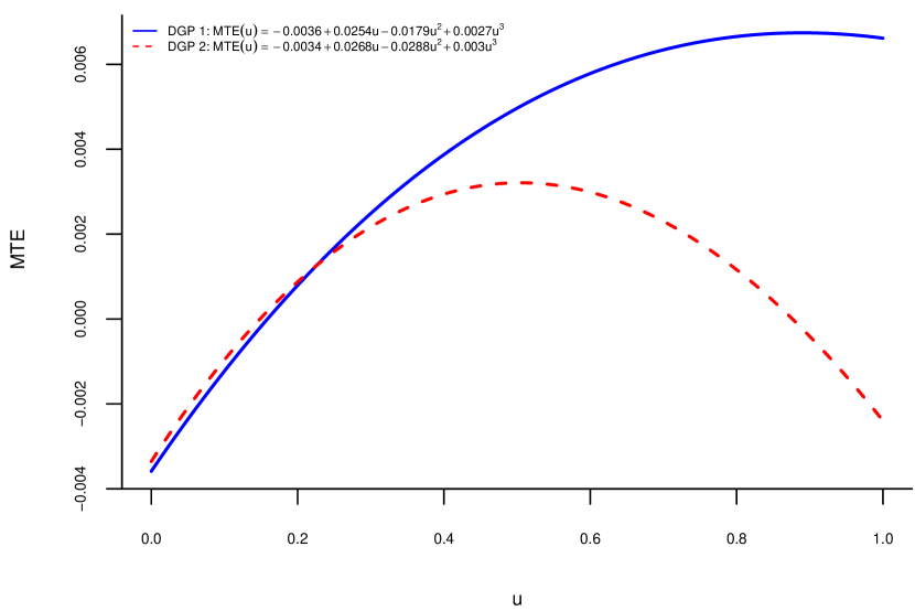
   Figure 2: Simulated DGPs from Study 4

4. Simulating the multi-cell experiment. We use these MTE functions to simulate data from our experimental design with two cells. This design limits us to a linear approximation to $m_{1}(\cdot)$ and a quadratic approximation to $m_{0}(\cdot)$. First, we set the propensity scores in our simulated multi-cell experiment. Because Study 4 assigned users to be eligible to receive treatment with probability 0.7, we consider this to be one cell and add a second cell in which this probability equals 0.3. For the first cell we keep the propensity score at the original value, $\nu(Z_{1}=1)=0.37$, and set the propensity score for the second cell so that $\Pr(Z_{1}=1|C=1)\times\nu(Z_{1}=1)=\Pr(Z_{2}=1|C=2)\times\nu(Z_{2}=1)$, implying that $\nu(Z_{2}=1)\approx 0.86$. We use these propensity scores and the underlying MTE functions to compute the $\psi$s from equations (3.2) and (3.2) that would have been observed had our design been implemented.

4.2 Results from our proposed approach

We use the $\psi$s from above to obtain the approximated MTE functions following the procedure we described in Section 3.3. The resulting approximations to the DGPs we consider are shown in Figure 3.

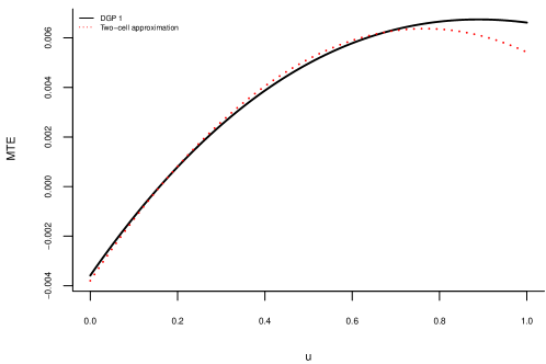
(a)

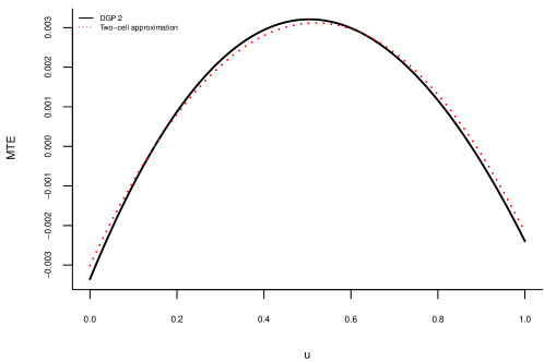
(b)

Figure 3: Approximations to simulated DGPs from Study 4

Although the underlying MTE functions are cubic, the fact that their shapes are close to quadratic implies that a two-cell design yields good approximations. We quantify the quality of these approximations through three metrics. Denote the approximation to the true MTE function by $\text{MTE}_{\text{app}}(\cdot)$. The metrics we consider are the sup-norm, $\max_{u\in[0,1]}\left|\text{MTE}(u)-\text{MTE}_{\text{app}}(u)\right|$, and the $L_{2}$-norm, $\sqrt{\left(\int_{0}^{1}\left[\text{MTE}(u)-\text{MTE}_{\text{app}}(u)\right]^{2}du\right)}$. In addition, we consider the quality of the approximated ATE, $\text{ATE}_{\text{app}}$, relative to the true value, which we refer to as “ATE-norm:” $\frac{\text{ATE}_{\text{app}}-\text{ATE}}{\text{ATE}}$. We consider this metric as a different way of summarizing the discrepancy between the true and approximated MTE functions because often the ATE is the treatment effect parameter of original interest to the researcher.

The results are given in Table 1. Overall, our method generates a small difference between the approximations and their true values. For example, it produces a relative error in the estimated ATEs of about -3% and 2% for each of the DGPs, respectively.

Table 1: Distance between true and approximated MTE functions: two-cell design

Metric	DGP 1	DGP 2
sup-norm	0.00019	0.00015
$L_{2}$-norm	0.00036	0.00014
ATE-norm	-0.03009	0.02432

4.3 Implications for decision-making

We consider the firm’s decision problem given in equation (7). For the sake of illustration, we set $\delta=1$ and $\kappa(\nu)=0.001\nu^{4}$. A firm can set $\delta$ based on their internal assessment of the value of a conversion event. We specify $\kappa(\nu)$ as convex to capture the notion that reaching the marginal consumer becomes more expensive as overall campaign reach increases. As we note in Section 2.1, most advertising platforms provide advertisers with campaign planning tools to help them predict how reach is expected to vary as a function of their budget. Based on the simulated DGPs we outlined above, the resulting expected profit functions are given in Figure 4.

The expected profit functions reflect the differences across the different DGPs shown in Figure 2. They demonstrate how different MTE functions can affect optimal decisions. In this case, the optimal decisions associated with DGPs 1 and 2 are to treat 100% and 75.5% of the population, respectively.

We now compare the true optimal solutions to what the decision-maker would do if information obtained from our experimental design was available, following the Bayesian estimation procedure we presented in Section 3.4. That is, we consider solutions to (3.4). The third column of Table 2, “Multi-cell,” shows the expected profit losses from using the method we propose.

The multi-cell approach yields virtually no losses across both DGPs, and is able to identify the true optimal solution correctly under DGP 1. This is perhaps unsurprising given that it was able to approximate the underlying MTE functions well.

A pertinent question, however, is whether direct applications of BMW could provide comparatively good decisions. If so, they would be arguably preferable relative to our method given that the usual design with one-sided non-compliance is simpler. We address this matter next.

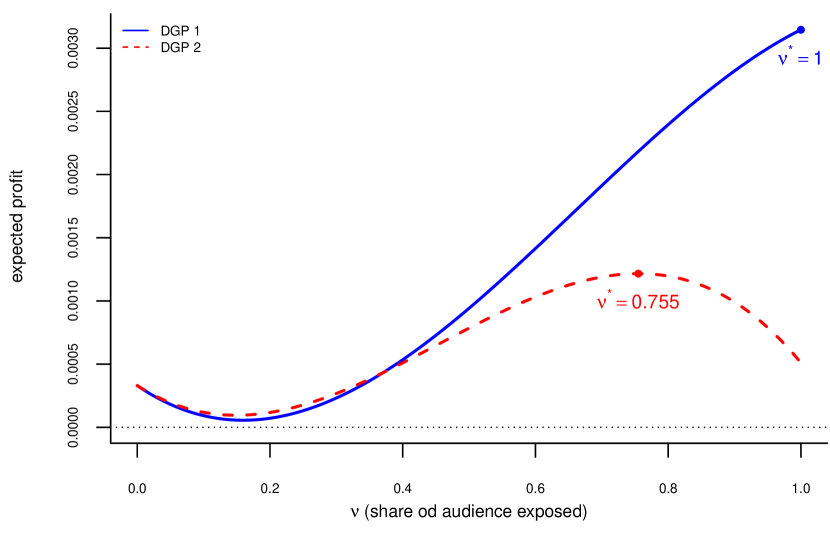
Figure 4: Expected profit functions from simulated DGPs of Study 4

Table 2: Decisions from approximated expected profit functions

DGP	True $\nu^{*}$	Multi-cell		$\lambda_{11}=0$		$\lambda_{11}=\lambda_{01}$		$\lambda_{10}=0$		$\lambda_{10}=\lambda_{00}$
		$\nu^{*}$	Loss	$\nu^{*}$	Loss	$\nu^{*}$	Loss	$\nu^{*}$	Loss	$\nu^{*}$	Loss
1	1	1	0	0.484	0.723	0.432	0.792	1	0	0.661	0.454
2	0.755	0.762	0.0003	0.484	0.391	0.432	0.509	1	0.58	0.661	0.061

4.4 Direct application of BMW’s method with only one cell

BMW’s method can be applied to data obtained from the typical experimental design. However, because this design yields one-sided noncompliance, $\nu(0)=0$ while $\nu(1)\in(0,1)$. Thus, equations (3.3) and (3.3) imply that the only moments identified from the data it provides are $\psi_{11}$, $\psi_{01}$ and $\psi_{00}$, where we omit the subscript $c$ to ease notation since there is only one cell. Based on the logic from equations (16) and (17), these moments allow us to approximate $m_{1}(\cdot)$ with a constant function and $m_{0}(\cdot)$ with a linear function. Consequently the MTE function itself can be approximated with a linear function.

The ability to approximate the MTE function with a linear function might seem attractive, especially because it is not uncommon to maintain the assumption that the MTE function is indeed linear. Nevertheless, the missingness of $\psi_{10}$ implies that this approximation inherently features a restriction that nontrivially impacts not only the quality of the approximation, but also the structure of the endogeneity of treatment.

To see this, suppose for simplicity that $m_{d}(u)=\lambda_{d0}+\lambda_{d1}u$ for $d\in\{0,1\}$. It follows that:

$$\mathbb{E}\left[Y\middle|D=1,Z=z\right] =\lambda_{10}+\frac{\lambda_{11}}{2}\nu(z)$$

$$\mathbb{E}\left[Y\middle|D=0,Z=z\right] =\left(\lambda_{00}+\frac{\lambda_{01}}{2}\right)+\frac{\lambda_{01}}{2}\nu(z).$$

The data obtained from the typical experimental design thus enable us to recover $\lambda_{00}$ and $\lambda_{01}$. Nevertheless, they do not allow us to recover $\lambda_{10}$ and $\lambda_{11}$ separately because we do not observe $\psi_{10}$. This is an underidentification problem: there are four parameters to be estimated ($\lambda_{10}$, $\lambda_{11}$, $\lambda_{00}$ and $\lambda_{01}$) but only three moments available to estimate such parameters ($\psi_{11}$, $\psi_{01}$ and $\psi_{00}$). To make progress, therefore, the researcher must impose an additional restriction on the parameters.

Unfortunately, we are unaware of any general theory or methodology that can provide clear guidance on such restriction, although progress has been recently made in this direction (e.g., Kowalski, 2023a, ). Whichever restriction is chosen, a key point is that such additional constraint must always be imposed to implement BMW’s estimator using data collected from an experiment with one-sided noncompliance, which, to our knowledge, has not been noted in the literature. Given the pervasiveness of such experimental designs, we hope our approach provides a valuable solution to recover the MTE function more credibly.

For the purposes of comparing our approach to a direct application of BMW, we consider four possible restrictions. First, in accordance with the approximation method from Section 3.3, we consider approximating $m_{1}(\cdot)$ with a constant, that is, imposing that $\lambda_{11}=0$, which enables the estimation of $\lambda_{10}$. From a purely mechanical perspective, the higher $|\lambda_{11}|$ is, the lower the quality of the approximation. However, the constraint $\lambda_{11}=0$ also has a deeper structural implication. It implies that all endogeneity stems from $Y_{0}$. This rules out certain forms of self-selection, such as the classic case of $D=\mathbb{1}\left\{Y_{1}\geq Y_{0}\right\}$, where only units that benefit from treatment are treated. In our setting of online advertising, this precludes “perfect” ad exposure where units are exposed to the ad only if this benefits the advertiser.

The second restriction we consider it to set $\lambda_{11}=\lambda_{01}$, thereby ruling out endogeneity altogether but also allowing us to recover $\lambda_{10}$. However, this is often considered implausible, including in the context of online advertising.

Third, we impose $\lambda_{10}=0$, which allows us to recover $\lambda_{11}$. Given linearity, this restriction implies that $m_{1}(\cdot)$ is either always negative or always positive, which can be justified in cases where $Y_{1}$ is bounded either from above or below at 0. The same can be achieved for the MTE function by imposing that $\lambda_{10}=\lambda_{00}$, while also enabling the estimation of $\lambda_{11}$.

Table 2 also shows the optimal decisions and expected profit losses from using BMW’s method directly under each of these constraints. The results do not show a systematic pattern. Notice that setting $\lambda_{10}=0$ eliminates expected profit losses under DGP 1, which the multi-cell approach also does.

However, the decisions implied by the different versions of BMW do not vary across DGPs. To the extent that DGPs differ, and thus their implied optimal decisions, so will the performance of these different versions of BMW depending on what the true DGP is. As Figure 4 shows, the optimal solutions under DGPs 1 and 2 are quite different. Imposing $\lambda_{10}=0$ would yield high losses under DGP 2, as expected. Under such DGP, the best version of the direct application of BMW among the ones we consider is the one that sets $\lambda_{10}=\lambda_{00}$; however, this version, unsurprisingly, performs poorly under DGP 1.

5 Implementing the multi-cell experiment

This section provides some guidance for how researchers (or an ad platform) might implement our experimental design in practice. First, we discuss the main set of implementation requirements for the model. Second, we address the fact that many ad campaigns entail multiple advertising exposures, whereas our model assumes treatment is binary. Third, we explain how certain strong functional form assumptions yield precise prescriptions for the number of cells and propensity score values. We highlight how similar guidance under weaker assumptions is more difficult.

5.1 Testing Requirements

Implementing our multi-cell experimental design in practice requires knowledge of certain inputs for the model and access to the appropriate experimentation service on an advertising platform. We discuss each of these in more detail below. Importantly, our proposed design does not require additional budget to be implemented relative to the usual experiment design that randomizes eligibility to receive treatment.

One key input to our model is the monetary value of an outcome, $\delta$. For “direct response” campaigns, in which the advertiser has a particular outcome in mind, for example, to increase sales of a product, $\delta$ would be the average profit margin on products sold through the campaign. This quantity should be known, or estimable, to the advertiser. Most ad platforms allow advertisers to programatically connect outcomes with their monetary conversion values so that all reporting reflects this information. Although outcomes with direct monetary values are the most natural fit for our model, any outcome that the advertiser deems of value could work provided that the advertiser can assign a monetary value to the outcome.

The second key input is the cost of treating a fraction $\nu$ of the target audience, $\kappa(\nu)$. Platforms share information with advertisers that can be used to estimate $\kappa(\cdot)$ when they set up their campaigns. Common campaign planning tools present predicted campaign reach (in terms of users) as a function of budget, conditional on audience targeting parameters. This allows the advertiser to understand the fraction of the audience that they can expect to reach for a particular budget choice, $B$, or effectively, to understand $\nu=\kappa^{-1}(B)$.

The advertising platform must be capable of implementing multi-cell experiments with sufficient flexibility in their configuration. If the platform creates separate test/control splits within each cell (as Meta does), it must allow for either different splits across cells while keeping the budget per cell fixed or different budgets across cells. This flexibility is necessary to create the appropriate variation in $\nu(Z_{c}=1)$. Similarly, if the platform creates one control group and $C$ test groups, which is equivalent to our design, then our method requires flexibility in the relative size of each group or the budget allocation across groups.

To create variation in $\nu(Z_{c}=1)$ across cells, the goal is to create variation in the (expected) budget per user. For simplicity, normalize the size of the target audience to one and let a fraction $\Pr(\mathcal{C}=c)$ be randomly allocated to cell $c$. Denote the total budget allocated to this cell by $B_{c}$. Then, the budget per user in cell $c$ is $\tilde{B}_{c}=\frac{B_{c}}{\Pr(Z_{c}=1|\mathcal{C}=c)\times\Pr(\mathcal{C}=c}$, such that $\nu(Z_{c}=1)=\kappa^{-1}\left(\tilde{B}_{c}\right)$. Hence, the experimenter can vary the budget per user by (i) allocating different fractions $B_{c}$ of the original budget, $B$, (ii) choosing different values for $\Pr(Z_{c}=1|\mathcal{C}=c)$, or (iii) assigning different fractions of users to the different cells, $\Pr(\mathcal{C}=c)$. Thus, the experimenter is able to generate variation in the budget per user across cells, which, in turn, generates variation in $\nu(Z_{c}=1)$ through the function $\kappa(\cdot)$. We discuss this intuition in more detail in Appendix D and the challenge of optimally choosing $C$ and $\nu(Z_{c})$ in Section 5.3.

After the experiment is complete, the platform must report $\psi_{dzc}$ and $\nu(Z_{c}=1)$. Note that these quantities are aggregated, such that they do not require access to any individual-level data.

5.2 Addressing multiple advertising exposures

The approach we took casts advertising as a binary treatment variable and assumes away the existence of multiple ad exposure effects. If these effects exist, then this approach is inadequate. One possible alternative is to incorporate the number of previous exposures as a covariate into the model, which we do in Appendix A. Here, we provide a more informal discussion of the consequences of ignoring multiple exposures.

When these exposures are relevant but ignored, the exclusion restriction given in Assumption 1 is violated. To see this, notice that, if ignored, these exposures become part of the error term associated with the potential outcomes. At the same time, they are correlated with the instrument: if different cells are associated with different budgets, which can thus be seen as the instrument, then higher budgets should be associated with higher number of impressions.

However, as we illustrate in Appendix A, ignoring the total number of impressions can be inconsequential when their effect is negligible. Whether this is the case depends on the specific setting.

One example where ignoring repeated exposures might be reasonable are settings with low frequency caps, because they induce a low number of impressions per user overall. Even though all major ad platforms make frequency caps available (e.g., The Trade Desk, Google’s DV 360, and Amazon Advertising), there is little agreement in the industry on whether this number should be high or low. For example, an analysis by Meta found that “a frequency cap of at least 1 to 2 per week was able to capture a substantial portion of the total potential brand impact.” This is roughly consistent with a paper by Yuan et al., (2013). The Trade Desk offers substantially different guidance, while cautioning that there is no one-size-fits-all approach to setting frequency caps. Ultimately, we think advertisers should test out different frequency caps to understand what is best for them (Forbes,, 2019).

Whether repeated exposures are significant also depends on the specific outcome variable. Research on this topic remains relatively scarce. Sahni, (2015) finds significant effects on calls to restaurants. In turn, Johnson et al., (2016) finds significant effects on sales when imposing certain functional forms, but more flexible specifications cast doubt on this finding. Lewis, (2014) examines 30 ad campaigns on Yahoo and finds mixed evidence of repeated ad exposure effects on click-through rates. Sahni et al., (2019) find some evidence of frequency on visits at one online retailer.

Overall, it is difficult to explicate the specific conditions of an ad campaign that are likely to generate repeated exposure effects. To our knowledge, the literature has not been able to detect effects of repeated exposures on purchases, which is the outcome variable of the Facebook experiment we use in our simulation. This suggests that the approach that casts advertising as a binary treatment may be appropriate when this is the outcome of interest. Otherwise, if a researcher feels multiple exposures are important, then so long as they (or the ad platform) can collect the necessary data, they could instead apply our extended model that conditions on exposure count to maintain the validity of the exclusion restriction.

5.3 Choosing the number of cells and propensity score values

The choice of $C$ and $\nu(Z_{c}=1)$ are key design elements of our approach, taking the budget for the experiment as given. Unsurprisingly, the extent to which there can be clear guidelines for these choices depends on the nature of the approximation desired, which, in turn, should arguably be a function of the assumptions made about the underlying DGP.

As we discussed in Section 4.4, a common approach is to assume that the MTR functions are linear, or to approximate them with a linear function. The requirement to obtain such an approximation is to observe two values of $\nu(\cdot)$ that are different from each other and strictly between zero and one. This can be accomplished with a two-cell design with an unequal allocation of the overall budget to each cell. In theory, any two values of $\nu(\cdot)$ suffice to obtain this linear approximation.

A different approach that can also be implemented with just two different values of $\nu(\cdot)$ is the one used, for example, by Heckman et al., (2001, 2003): to assume an underlying DGP featuring a normal distribution. Under this assumption, the method to compute the MTR functions is no that of BMW; however, our proposed multi-cell design can still be used with this different estimation method. We consider this specific case in Appendix A, which, like the linear case, features monotone MTR functions.

Without such strong functional form assumptions, however, it becomes difficult to obtain clear guidelines on how to choose $C$ or $\nu(Z_{c}=1)$. In Appendix F, we consider MTE functions that are monotonic or that satisfy the assumption of monotone treatment response (Manski,, 1997). We find that these assumptions do not necessarily produce sufficiently “well-behaved” MTE functions so as to enable precise guidance. We leave to additional work on how to best leverage such assumptions.

Another practical concern is estimation precision. With a finite number of units (consumers), the choice of the number of cells in the experiment creates a type of bias-variance trade-off. More cells generate more values of the propensity score, theoretically enabling a more flexible approximation of the MTE function, and thus decreasing bias. But as the number of units per cell decreases, the estimates of the approximating function will become noisier, and thus increasing variance. Hence, the number of cells can be seen as somewhat akin to the bandwidth in nonparametric estimation. Without strong assumptions on the underlying MTE function, it is not possible to establish how to make progress on the task of choosing the number of cells vis-à-vis the available sample size.

6 Conclusion

Experiments are considered an especially attractive tool to estimate the impacts of treatments and interventions. When treatment assignment cannot be randomized, a common approach is to randomize eligibility to receive treatment instead, leading to one-sided noncompliance. Nevertheless, decision-makers who conduct experiments are often interested in obtaining information to assist them in making specific decisions, and not just measuring the effects of treatment per se. Unfortunately, typical experimental designs, such as the one where eligibility to receive treatment is randomized, do not provide enough information to assist with many decisions.

This paper proposed an approach to obtain such information. This approach combines a novel multi-cell experimental design and modern estimation techniques, where the former leads to the collection of data that contain more information about treatment effects and the latter exploits this information. Our approach leverages the method from Brinch et al., (2017), which we point out requires an arbitrary additional assumption to be applied to experiments with one-sided noncompliance.

Using data from an online advertising experiment at Facebook, we addressed the performance of our proposed multi-cell experimental design vis-á-vis that of the typical experimental design. To do so, we implemented the aforementioned estimators on simulated data that was calibrated based on this experiment. We found that the decisions obtained from our design yield lower losses in expected profit than those from the typical design.

6.1 Limitations and Future Research

Three natural questions arise in the context of many approximations. Fist, to what extent can the approximated MTE function be used be generalized beyond the specific audience and ad platform on which it was obtained? In Appendix A, we extend our model to condition on a scalar $X$ that we interpret as being the number of previous exposures for a user. However, it might be possible to further generalize this specification to make $X$ vector valued. Allowing for a rich enough set of conditioning variables in $X$ might be one way to help generalize the estimated MTE function to other advertising contexts.

Second, is there a way to intelligently choose the number of cells and propensity score values? Intuitively, the higher the number of cells and the more variation there is in the propensity score values, the better. Nevertheless, the quality of the resulting approximations depends crucially on the underlying DGP. Without strong restrictions, such as the normality assumption discussed in Section 5.3, it is difficult to obtain specific guidance for these choices. Furthermore, the precision of the estimator of the approximate MTE function should be taken into account. For a given sample size, the number of cells creates a bias-variance tradeoff, and using a framework based on this tradeoff could be a convenient way to inform this choice. In turn, the choice of propensity score values is akin to the choice of knot values for numerical integration, with the added component that the obtainable values depend on the budget; for example, a higher budget per user is required to obtain a higher exposure rate, that is, a high value for the propensity score. Incorporating this additional component to the problem adds yet another layer of complexity.

Third, are there additional reasonable restrictions that might improve the quality of the approximation? Imposing theory-based restrictions on the underlying DGP might be a way to make progress on obtaining theoretical bounds on the quality of the approximation even when ignoring estimation and monetary concerns. Ideally, such restrictions would impose enough structure to imply a “well-behaved” MTE function, whose properties could then be leveraged for approximation. To this end, we considered two commonly made and interpretable assumptions, monotone treatment response and monotonicity of the MTE function, but found that they are insufficient to generate a DGP whose properties can be exploited for approximation. One possible alternative for future research is to replace the polynomial approximation with more flexible functional forms that can better leverage and incorporate these restrictions.

It is possible that having access to one or more real multi-cell tests could help guide us to solutions to some of these questions. However, lacking a real multi-cell test, we do not have any information about what a true DGP would look like in terms of the resulting MTE. This makes it impossible for us to assess the true quality of our approximation, since we do not know if our assumed DGP bears any resemblance to a true DGP. We chose polynomials because this method is consistent with Brinch et al., (2017), possesses analytic integrals, and has favorable approximating properties. Any approximation method that is well-defined on the unit interval could potentially work (e.g., Bernstein polynomials). However, without any knowledge of a real-world DGP, it is hard to assess the relative accuracy of one approximation technique over the other. After running a sufficient number of multi-cell tests, an advertising platform could attempt to characterize common features and functional forms of the resulting MTEs to provide some guidance on preferred approximation methods.

Appendix A Dealing with multiple ad exposures

A.1 General incorporation of observable characteristics

We now demonstrate how to incorporate observable characteristics, captured in a vector $X$, into the model above. Three changes have to be made. First, equation (3) is replaced with:

$$D =\mathbbm{1}\left\{\nu(Z,X)\geq U\right\}.$$ (A.1)

Importantly, notice that the error in the selection, $U$, remains additively separable.

Second, Assumption 1 is replaced with:

Assumption A.1.

(i) $U\mathchoice{\mathrel{\hbox to0.0pt{$\displaystyle\perp$\hss}\mkern 2.0mu{\displaystyle\perp}}}{\mathrel{\hbox to0.0pt{$\textstyle\perp$\hss}\mkern 2.0mu{\textstyle\perp}}}{\mathrel{\hbox to0.0pt{$\scriptstyle\perp$\hss}\mkern 2.0mu{\scriptstyle\perp}}}{\mathrel{\hbox to0.0pt{$\scriptscriptstyle\perp$\hss}\mkern 2.0mu{\scriptscriptstyle\perp}}}Z|X$, where $\mathchoice{\mathrel{\hbox to0.0pt{$\displaystyle\perp$\hss}\mkern 2.0mu{\displaystyle\perp}}}{\mathrel{\hbox to0.0pt{$\textstyle\perp$\hss}\mkern 2.0mu{\textstyle\perp}}}{\mathrel{\hbox to0.0pt{$\scriptstyle\perp$\hss}\mkern 2.0mu{\scriptstyle\perp}}}{\mathrel{\hbox to0.0pt{$\scriptscriptstyle\perp$\hss}\mkern 2.0mu{\scriptscriptstyle\perp}}}$ denotes conditional statistical independence.
(ii) $\mathbb{E}\left[Y_{d}\middle|Z,X,U\right]=\mathbb{E}\left[Y_{d}\middle|X,U\right]$ and $\mathbb{E}\left[Y_{d}^{2}\right]<\infty$ for $d\in\{0,1\}$.
(iii) $U$ is continuously distributed conditional on X.

Finally, we replace Assumption 2 with:

Assumption A.2.

(i) $\Pr(Z_{c}=z|X,\mathcal{C}=c)\in(0,1)$ for all $X$, $c$ and all $z$.
(ii) $\nu(Z_{c}=1|X)\equiv\Pr\left(D=1\middle|X,Z_{c}=1\right)\in(0,1)$ for all $c$ and $X$.
(iii) $\nu(Z_{c}=1|X)\neq\nu(Z_{c^{\prime}}=1|X)$ for all $c\neq c^{\prime}$ and $X$.

In summary, Assumptions A.1 and A.2 simply add conditioning on $X$ to Assumptions 1 and 2. The equivalence between this model and that of Imbens and Angrist, (1994) remains. Furthermore, the MTR and MTE functions become $m_{d}(u,x)\equiv\mathbb{E}\left[Y_{d}\middle|U=u,X=x\right]$, where $d\in\{0,1\}$, and $\text{MTE}(u,x)\equiv\mathbb{E}\left[Y_{1}-Y_{0}\middle|U=u,X=x\right]=m_{1}(u,x)-m_{0}(u,x)$ , respectively.

A.2 Number of previous ad exposures as a covariate

In certain cases, one can expect that multiple exposures to an ad can have a significant impact on outcomes. We now show how multiple ad impression opportunities can be incorporated as a covariate into our setup.

To this end, assume that each user can be exposed to the ad $S$ times. We index all variables by $s=1,\dots,S$, to indicate that they are associated with impression opportunity $s$. We define $X_{s}$ as the number of times the user was exposed to the ad prior to impression opportunity $s$.

To generate variation in the probability of exposures and in the number of previous ad exposures, we treat $Z$ as the budget designated to each user, which is the same for all users within a cell but varies across cells. As the advertiser shows their ad over impression opportunities, this budget diminishes due to the auction payments. We denote the remaining available budget at impression opportunity $s$ by $Z_{s}$.

We follow the model with essential heterogeneity from Heckman et al., (2006):

$$\begin{split}Y_{1s}&=\mu_{1}(X_{s})+\epsilon_{1s}\\ Y_{0s}&=\mu_{0}(X_{s})+\epsilon_{0s}\\ D_{s}&=\mathbbm{1}\left\{\nu(Z_{s},X_{s})\geq U_{s}\right\}\end{split}$$ (A.2)

where, conditional on $X_{s}$, $\epsilon_{1s}$, $\epsilon_{0s}$ and $U_{s}$ are i.i.d. across $s$ following some joint distribution. Consequently, the MTR functions take the form:

$$m_{d}(u,x)=\mu_{d}(x)+\mathbb{E}\left[\epsilon_{ds}\middle|U_{s}=u\right],$$ (A.3)

where $d\in\{0,1\}$.

The i.i.d. condition across $s$ deserves attention, especially regarding $U_{s}$. We interpret the variable $U$ as the ease with which a user can be exposed to the ad. Thus, it would be reasonable to expect that this term would be correlated across $s$. However, this would invalidate the available budget, $Z_{s}$, as an instrument for $D_{s}$, which is why we maintain this i.i.d. condition. This assumption could become more palatable if additional variables, such as user and impression opportunity characteristics, were incorporated into $X$. However, this is a caveat that should be taken into consideration.

A.3 Sequential approximations to MTE function

We propose a sequential approach that approximates the MTE function at each value of $X_{s}$ separately. This is motivated by the fact that: (i) online advertising experiments involve a large number of users; (ii) the data are often stored sequentially as they arrive for the duration of the experiment; and (iii) the only variable we are including in $X_{s}$ is the previous number of impressions. Should other variables be included in the model, alternative approaches can also be considered.

Using a multi-cell experimental design with sequential storage of data allows us to recover the following moments:

$$\psi_{1zx} =\mathbb{E}\left[Y\middle|D_{s}=1,X_{s}=x,Z_{s}=z\right]$$

$$=\mathbb{E}\left[Y_{1}\middle|U_{s}\leq\nu(z,x),X_{s}=x,Z_{s}=z\right]$$

$$=\mu_{1}(x)+\frac{1}{\nu(z,x)}\int_{0}^{\nu(z,x)}\mathbb{E}\left[\epsilon_{1s}\middle|U_{s}=u\right]du$$ (A.4)

and

$$\psi_{0zx} =\mathbb{E}\left[Y\middle|D_{s}=0,X_{s}=x,Z_{s}=z\right]$$

$$=\mathbb{E}\left[Y_{1}\middle|U_{s}>\nu(z,x),X_{s}=x,Z_{s}=z\right]$$

$$=\mu_{0}(x)+\frac{1}{1-\nu(z,x)}\int_{\nu(z,x)}^{1}\mathbb{E}\left[\epsilon_{0s}\middle|U_{s}=u\right]du.$$ (A.5)

Hence, we can approximate the MTE function at each value of $x$ separately using $\psi_{1zx}$, $\psi_{0zx}$, and $\nu(z,x)$ following the procedure described in Section 3.3.

This procedure has an important feature. As impressions are obtained, the available budget decreases; that is, the number of different values of $Z_{s}$ decreases as $X_{s}$ increases. Consequently, the degree of the approximating polynomial is lower for higher values of previous exposures to the ad, rendering this approximation, at least theoretically, poorer.

A.4 Calibrated simulations with multiple exposures

We now describe the specification we chose for our calibrated simulations with multiple ad impression opportunities. This specification is motivated solely for simplicity, but the parameter values are chosen based on the data from the Facebook experiment we consider.

A.4.1 Distributional and parametric assumptions

To implement our calibrated simulations, we make the following normality assumption:

$$\begin{bmatrix}\epsilon_{1s}\\ \epsilon_{0s}\\ V_{s}\end{bmatrix}\Big{|}X_{s}\sim N\left(\begin{bmatrix}0\\ 0\\ 0\end{bmatrix},\begin{bmatrix}\sigma_{1}^{2}&\rho_{10}\sigma_{1}\sigma_{0}&\rho_{1V}\sigma_{1}\\ \rho_{10}\sigma_{1}\sigma_{0}&\sigma_{0}^{2}&\rho_{0V}\sigma_{0}\\ \rho_{1V}\sigma_{1}&\rho_{0V}\sigma_{0}&1\end{bmatrix}\right)$$ (A.6)

where $V_{s}=\Phi^{-1}(U_{s})$ and where $\Phi(\cdot)$ denotes the cdf of the standard normal distribution. We further assume that:

$$\mu_{d}(x)=\mu_{d0}+\mu_{d1}x+\mu_{d2}x^{2}$$ (A.7)

where $d\in\{0,1\}$. Consequently, we obtain:

$$m_{d}(x,u)=\mu_{d0}+\mu_{d1}x+\mu_{d2}x^{2}+\rho_{dV}\sigma_{d}\Phi^{-1}(u).$$ (A.8)

The normality assumption in (A.6) is oftentimes maintained and is of great aid in identifying and estimating the MTE function. As discussed, for example, in Mogstad and Torgovitsky, (2018), all that is necessary to recover $\rho_{dV}\sigma_{d}$, where $d\in\{0,1\}$, is for the propensity score to have two distinct values between 0 and 1 at just one value of $x$. Consequently, with enough variation in $x$ to estimate $\mu_{d}(\cdot)$ it is possible to recover the entire MTR functions under this weaker condition.

However, this convenience also imposes non-trivial restrictions on the model. For instance, it imposes that the MTR functions are monotonic in $u$, ruling out the DGPs we considered in Section 4, and that they tend to plus and minus infinity at the extremes of the unit interval, as depicted in Figure A.1. On the other hand, the approach of approximating the MTR functions with polynomials from BMW is agnostic and does not impose such restrictions on the DGP.

A.4.2 Features of simulated experiment

First, we set $S=3$. In practice, the number of potential ad impressions can be much larger and is a function of the duration of the experiment. We choose a low value solely for simplicity. In addition, such reduction is sometimes implemented in practice via bracketing. For instance, $s=1$ can correspond to the first five impressions, $s=2$ to the following five, and so on.

Second, we assume that:

$$\nu(Z_{s},X_{s})=\frac{Z_{s}}{Z_{s}+t},$$ (A.9)

where $t>0$. This is a simple way of ensuring that the probability of exposing a user to the ad is zero when there is no budget left, that is, when $Z_{s}=0$. We choose the parameter $t$ to generate variation in the propensity score across the different values of $Z_{s}$. Also, notice that this probability does not depend on $X_{s}$, a choice we made solely for simplicity. $X_{s}$ could be easily incorporated into this propensity function via frequency caps.

Third, we assume that the experiment randomizes users into five groups determined by the initial budget allocated to them. In particular, we set $Z\in\left\{0,1,2,3,4\right\}$.

Finally, when the advertiser wins an impression opportunity, they make a payment and the available budget decreases. We simply assume that:

$$Z_{s+1}=\begin{cases}Z_{s}-1&\text{if }D_{s}=1\\ Z_{s}&\text{if }D_{s}=0\end{cases}$$ (A.10)

We choose the budget to decrease by one to facilitate the simulation by aligning the evolution of budget with the initial budget allocation. In practice, decreases in the available budget are determined by auction payments, which almost always vary across impression opportunities.

A.4.3 Choice of parameter values

Under this setup, we have to choose values for ten parameters: $\mu_{10}$, $\mu_{11}$, $\mu_{12}$, $\mu_{00}$, $\mu_{01}$, $\mu_{02}$, $\sigma_{1}$, $\sigma_{0}$, $\rho_{1V}$, and $\rho_{0V}$. To do so, we use data from the same Study 4 we considered in Section 4. It is important to recall that Study 4 only randomized eligibility to ad exposure and not budget levels.

We set $\sigma_{d}^{2}=\text{Var}\left(Y\middle|Z=d\right)$, where $d\in\{0,1\}$, and obtain $\sigma_{1}=0.0185584$ and $\sigma_{0}=0.0158245$. Nevertheless, it is important to note that, in practice, these equalities are unlikely to hold.

The data to which we have access to calibrate $\mu_{d}\equiv\left[\mu_{d0},\mu_{d1},\mu_{d2}\right]^{\prime}$, where $d\in\{0,1\}$, consist of the following moments: $\mathbb{E}\left[Y\middle|D=0,Z=0\right]$, $\mathbb{E}\left[Y\middle|D=0,Z=1\right]$, $\mathbb{E}\left[Y\middle|X=1\right]$, $\mathbb{E}\left[Y\middle|X=1\right]$, $\mathbb{E}\left[Y\middle|X=2\right]$, and $\mathbb{E}\left[Y\middle|X=3\right]$. These expressions and their interpretation warrant a few comments.

We only have access to aggregate results at the end of the experiment, but not to the sequential evolution of results. Thus, $Y$ and $X$ are the observed outcomes and total number of ad exposures, respectively, at the end of the experiment. As a consequence, we omit the conditioning on $X$ when $D=0$ because, by construction, it is equal to zero. Furthermore, also by construction, $X>0$ if and only if $D=Z=1$, so we omit the conditioning on $D=1$ and $Z=1$ when $X>0$. Given this structure, we only have two moments informative of $m_{0}(\cdot)$, $\mathbb{E}\left[Y\middle|D=0,Z=0\right]$ and $\mathbb{E}\left[Y\middle|D=0,Z=1\right]$, and three moments informative of $m_{1}(\cdot)$, $\mathbb{E}\left[Y\middle|X=1\right]$, $\mathbb{E}\left[Y\middle|X=2\right]$, and $\mathbb{E}\left[Y\middle|X=3\right]$.

Given (A.8), evaluating (A.3) at $x=0$ yields two equations that allow us to estimate $\mu_{00}$ and $\rho_{0V}$. This is because we already calibrated $\sigma_{0}$ and because $\nu(0,0)$ and $\nu(1,0)$ are observed in the data from the numbers of observations associated with each $(Z,D,X)$ combination. Solving for these parameters yields $\mu_{00}=0.0002505$ and $\rho_{0V}=-0.006081128$. We then arbitrarily set $\mu_{01}=0.001$ and $\mu_{02}=-0.00075$ so that $m_{0}(\cdot)$ becomes concave in $x$.

Similarly, given (A.8), by equation (A.3) we have three equations. Since we already calibrated $\sigma_{1}$, we have four unknown parameters associated with $m_{1}(\cdot)$. We set $\rho_{1V}=0.3$ to induce endogeneity in treatment because we obtained a very low value for $\rho_{0V}$, which enables us to use these three equations to solve for $\mu_{1}$. We obtain $\mu_{10}=0.002443738$, $\mu_{11}=0.007943073$, and $\mu_{12}=-0.001791018$. Notice that these values imply that $m_{1}(\cdot)$ is also concave in $x$.

The resulting MTE function at $x\in\{0,1,2\}$ is displayed in Figure A.1. Because of additive separability, the MTE function does not cross at different values of $x$. While it is increasing in $x$, we can see that it is also concave.

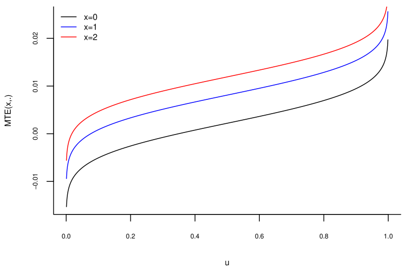
Figure A.1: MTE function with multiple exposures

A.4.4 Results

We now present the results of our calibrated simulations. We separate these results into two groups. First, we show the results from the sequential approach we described above. Second, we present the results from the procedure we described in Section 3, which ignores multiple ad exposures. We refer to this as the “naive approach.” All results are shown in Figure A.2.

Sequential approach

Figures LABEL:fig:mult_seq0$-$LABEL:fig:mult_seq2 show the approximations to the MTE function at different values of $x$ following the sequential procedure described above, depicting the MTE function with a solid line and the approximating polynomial with a dotted line. The method is able to approximate the MTE function well across all values of $x$ even though, as discussed above, the degree of the approximating polynomial decreases as $x$ increases.

(a)

(b)

(c)

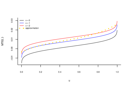
(d)

Figure A.2: Approximations to MTE function with multiple exposures

Naive approach

Figure LABEL:fig:mult_naive shows the MTE functions at different values of $x$ in solid lines and the naive approximation with a dotted line. This naive approximation, which ignores multiple exposures, resembles an approximation to an “averaged” over $x$ MTE function. Because the true function does not vary significantly between $x=1$ and $x=2$, this approximation is close to the true MTE function at these values, and especially at $x=1$. However, the approximation to the MTE function at $x=0$ is arguably poor.

The overall quality of the naive approximation is a reflection of the extent to which multiple exposures affect outcomes. Given our assumed DGP and calibration approach, repeated exposures do not seem to have a sizable impact. Since the outcome variable is an indicator for a purchase, this result is in accordance with results of the extant literature, which we discussed in Section 5.2. However, it is important to note that it is possible to choose a different DGP, also consistent with the observed data, where repeated exposures would have a strong impact on the outcome variable.

Appendix B Rewriting firm’s decision problem

We now demonstrate how the firm’s decision problem given in equation (2) can be rewritten as in equation (7). We begin by deriving the terms in equation (6). First, we have that:

$$\mathbb{E}\left[Y_{1}\middle|U\leq\nu\right] =\int_{0}^{\nu}\int_{y_{1}\in\mathcal{Y}_{1}}y_{1}\frac{f(y_{1},u)}{\Pr(U\leq\nu)}dudy_{1}$$

$$=\int_{0}^{\nu}\left(\int_{y_{1}\in\mathcal{Y}_{1}}y_{1}f(y_{1}|u)dy_{1}\right)\frac{f(u)}{\nu}du$$

$$=\int_{0}^{\nu}\mathbb{E}\left[Y_{1}\middle|U=u\right]\times\frac{1}{\nu}du$$

$$\equiv\int_{0}^{\nu}m_{1}(u)\frac{1}{\nu}du,$$ (B.1)

where in the third equality we used that $U\sim U(0,1)$ and defined $m_{1}(u)\equiv\mathbb{E}\left[Y_{1}\middle|U=u\right]$. Second,

$$\mathbb{E}\left[Y_{0}\middle|U>\nu\right] =\int_{\nu}^{1}\int_{y_{0}\in\mathcal{Y}_{0}}y_{0}\frac{f(y_{0},u)}{\Pr(U>\nu)}dudy_{0}$$

$$=\int_{\nu}^{1}\left(\int_{y_{0}\in\mathcal{Y}_{0}}y_{0}f(y_{0}|u)dy_{0}\right)\frac{f(u)}{1-\nu}du$$

$$=\int_{\nu}^{1}\mathbb{E}\left[Y_{0}\middle|U=u\right]\times\frac{1}{1-\nu}du$$

$$\equiv\int_{\nu}^{1}m_{0}(u)\frac{1}{1-\nu}du,$$ (B.2)

where in the third equality we also used that $U\sim U(0,1)$ and defined $m_{0}(u)\equiv\mathbb{E}\left[Y_{0}\middle|U=u\right]$.

Plugging equations (B) and (B) back into expression (2) yields:

$$\max_{\nu\in[0,1]}\left(\delta\times\left\{\int_{0}^{\nu}m_{1}(u)du+\int_{\nu}^{1}m_{0}(u)du\right\}-\kappa(\nu)\right)$$

$$\max_{\nu\in[0,1]}\left(\delta\times\int_{0}^{1}m_{0}(u)du+\delta\times\left\{\int_{0}^{\nu}\left[m_{1}(u)-m_{0}(u)\right]du\right\}-\kappa(\nu)\right)$$

$$\max_{\nu\in[0,1]}\left(\delta\times\mathbb{E}\left[Y_{0}\right]+\delta\times\int_{0}^{\nu}\text{MTE}(u)du-\kappa(\nu)\right)$$

$$\max_{\nu\in[0,1]}\left(\delta\times\int_{0}^{\nu}\text{MTE}(u)du-\kappa(\nu)\right),$$

which establishes expression (7).

Appendix C Posterior distribution of approximation parameters

We now describe how to obtain draws from $p\left(\lambda_{1},\lambda_{0}\middle|\text{data}\right)$. To this end, we need to set priors over $\psi$ and $\nu$, denoted by $q(\psi,\nu)$, and the likelihood function of the data, $\ell\left(Y,D\middle|\mathcal{C},Z;\psi,\nu\right)$. We condition on $Z$ and $\mathcal{C}$ because they are randomly chosen.

We need to consider two cases. First, notice that because $D=0$ when $Z_{c}=0$ for all $c$, we can pool all observations such that $Z_{c}=0$ from all cells and use them to obtain the posterior distribution of $\psi_{00}$, as given in equation (3.2), conditional on the data. More precisely, given a prior distribution $q(\psi_{00})$ and the likelihood $\ell(Y|Z=0;\psi_{00})$, we can derive the posterior $p(\psi_{00}|Y,Z=0)$. The form of this distribution clearly depends on what type of variable $Y$ is. In our application below, $Y$ is binary. Hence, for convenience we set:

$$\begin{split}&Y|Z=0;\psi_{00}\sim\text{Bernoulli}\left(\psi_{00}\right)\\ &\psi_{00}\sim\text{Beta}(\alpha_{0},\beta_{0})\end{split}$$ (C.1)

which implies that

$$\begin{split}&\psi_{00}|Y,Z=0\sim\text{Beta}\left(\alpha_{0}+\sum_{i:Z_{ic}=0}Y_{i},n_{0}-\sum_{i:Z_{ic}=0}Y_{i}+\beta_{0}\right),\end{split}$$ (C.2)

where $n_{0}$ is the total number of ineligible users.

The second case conditions on $\mathcal{C}=c$ and $Z_{c}=1$. Denote the number of observations in this set by $n_{c}$. For convenience, we proceed in two steps, relying on the factorization:

$$\begin{split}\ell\left(Y,D\middle|\mathcal{C}=c,Z_{c}=1;\psi_{11c},\psi_{01c},\nu(z_{c})\right)&=\ell\left(Y\middle|D,\mathcal{C}=c,Z_{c}=1;\psi_{d1c}\right)\\ &\qquad\times\ell\left(D\middle|\mathcal{C}=c,Z_{c}=1;\nu(z_{c})\right)\end{split}$$ (C.3)

First, recall that $D$ is binary, so we proceed as above:

$$\begin{split}&D|Z_{c}=1,\mathcal{C}=c;\nu(z_{c})\sim\text{Bernoulli}\left(\nu(z_{c})\right)\\ &\nu(z_{c})\sim\text{Beta}(\alpha_{Dc},\beta_{Dc})\\ &\nu(z_{c})|D,Z_{c}=1,\mathcal{C}=c\sim\text{Beta}\left(\alpha_{Dc}+\sum_{i:Z_{ic}=1,\mathcal{C}_{i}=c}D_{i},n_{c}-\sum_{i:Z_{ic}=1,\mathcal{C}_{i}=c}D_{i}+\beta_{Dc}\right).\end{split}$$ (C.4)

The second step consists of obtaining the posterior distribution of $\psi_{d1c}$, as given in equations (3.2) and (3.2), conditional on the data. Once again, the form of this distribution clearly depends on what type of variable $Y$ is. Given our application, we proceed as in (C.1) and (C.2). Denote the number of observations such that $D=d$, $Z_{c}=1$ and $\mathcal{C}=c$ by $n_{d1c}$. Then:

$$\begin{split}&Y|D=d,Z_{c}=1,\mathcal{C}=c;\psi_{d1c}\sim\text{Bernoulli}\left(\psi_{d1c}\right)\\ &\psi_{d1c}\sim\text{Beta}(\alpha_{d1c},\beta_{d1c})\\ &\psi_{d1c}|Y,D=d,Z_{c}=1,\mathcal{C}=c\sim\text{Beta}\left(\alpha_{d1c}+\sum_{i:D_{i}=d,Z_{ic}=1,\mathcal{C}_{i}=c}Y_{i},n_{d1c}-\sum_{i:D_{i}=d,Z_{ic}=1,\mathcal{C}_{i}=c}Y_{i}+\beta_{d1c}\right).\end{split}$$ (C.5)

The approach we take is sequential: first, we obtains draws of $\nu$ and then, conditional on them, we draw $\psi$. Consequently, we avoid the feedback issue studied in Zigler et al., (2013).

Appendix D Distributing experiment budget across multiple cells

We now formally describe how the experimenter can distribute the experiment budget across multiple cells to generate the variation necessary to estimate the parameters of interest.

First, consider a two-cell experiment, and fix $\Pr(\mathcal{C}=1)$ and $\Pr(Z_{1}=1|\mathcal{C}=1)$. Let $\sigma_{1}$ be the fraction of the original budget, $B$, allocated to Cell 1, so that $B_{1}=\sigma_{1}\times B$. The effective budget for Cell 1 is then $\frac{B_{1}}{\Pr(Z_{1}=1|\mathcal{C}=1)\times\Pr(\mathcal{C}=1)}=\frac{\sigma_{1}}{\Pr(Z_{1}=1|\mathcal{C}=1)\times\Pr(\mathcal{C}=1)}\times B$, so that $\nu(Z_{1}=1)=\kappa^{-1}\left(\frac{\sigma_{1}}{\Pr(Z_{1}=1|\mathcal{C}=1)\times\Pr(\mathcal{C}=1)}\times B\right)$. Equivalently, we then obtain $B_{2}=(1-\sigma_{1})\times B$, so that the effective budget for Cell 2 becomes $\frac{B_{2}}{\Pr(Z_{2}=1|\mathcal{C}=2)\times(1-\Pr(\mathcal{C}=1))}=\frac{1-\sigma_{1}}{\Pr(Z_{2}=1|\mathcal{C}=2)\times(1-\Pr(\mathcal{C}=1))}\times B$ and $\nu(Z_{2}=1)=\kappa^{-1}\left(\frac{1-\sigma_{1}}{\Pr(Z_{2}=1|\mathcal{C}=2)\times(1-\Pr(\mathcal{C}=1))}\times B\right)$.

Hence, when running a two-cell design, given $B$ and $\kappa(\cdot)$, the experimenter has four decision variables: $\Pr(\mathcal{C}=1)$, $\sigma_{1}$, $\Pr(Z_{1}=1|\mathcal{C}=1)$ and $\Pr(Z_{2}=1|\mathcal{C}=2)$. For the desired variation in the propensity score to be generated, it is necessary that $\frac{\sigma_{1}}{\Pr(Z_{1}=1|\mathcal{C}=1)\times\Pr(\mathcal{C}=1)}\neq\frac{1-\sigma_{1}}{\Pr(Z_{2}=1|\mathcal{C}=2)\times(1-\Pr(\mathcal{C}=1))}$. Thus, the experimenter can always guarantee that this constraint is satisfied.

This framework can be generalized to $C$ cells in a straightforward manner. In this case, the experimenter has $3C-2$ variables: $\left\{\sigma_{c},\Pr(\mathcal{C}=c)\right\}_{c=1}^{C-1}$ and $\left\{\Pr(Z_{c}=1|\mathcal{C}=c)\right\}_{c=1}^{C}$, under the constraints that, for all $c=1,\cdots,C$, $\sigma_{c}\in[0,1]$, $\Pr(Z_{c}=1|\mathcal{C}=c)\in[0,1]$ and $\Pr(\mathcal{C}=c)\in[0,1]$, plus $\sum_{c=1}^{C}\sigma_{c}=1$ and $\sum_{c=1}^{C}\Pr(\mathcal{C}=c)=1$. To ensure that the propensity scores differ from one another, it is then required that $\frac{\sigma_{c}}{\Pr(Z_{c}=1|\mathcal{C}=c)\times\Pr(\mathcal{C}=c)}\neq\frac{\sigma_{c^{\prime}}}{\Pr(Z_{c^{\prime}}=1|\mathcal{C}=c^{\prime})\times\Pr(\mathcal{C}=c^{\prime})}$ for all $c\neq c^{\prime}$.

Appendix E A more complex DGP

We now consider a more complex MTE function to dig deeper into the ability of our proposed multi-cell experimental design to provide a good approximation of this function and to inform decision-making. In particular, we assess how the performance of our approach changes as the number of cells increases.

E.1 New MTE and expected profit functions

We choose $m_{1}(u)=\daleth\frac{1}{1+u}$ and $m_{0}(u)=\gimel\frac{1}{(1+u)^{2}}+\beth\sin^{2}(2\pi u)$. As before, the parameters $\daleth$, and $\beth$ and $\gimel$ are computed to match the observed $\psi_{11}$, $\psi_{01}$ and $\psi_{00}$. Figure E.1 depicts the resulting MTE function. We consider this function to be “complex” because is not monotonic, concave or convex over the entire domain.

Figure E.1: $\text{MTE}(u)=\daleth\frac{1}{1+u}-\gimel\frac{1}{(1+u)^{2}}-\beth\sin^{2}(2\pi u)$

Figure E.2 shows the implied expected profit function. Under this DGP, the optimal decision is to treat 91.54% of the population.

Figure E.2: Expected profit function under complex MTE

E.2 Approximations based on different numbers of cells

We now study how the quality of approximation changes as more cells are included into the experiment. In particular, in addition to the two-cell design, we consider three-cell and five-cell designs, which allow us to obtain cubic and quintic approximations to the MTE function, respectively. Cells 1 and 2 display the same eligibility probabilities and propensity scores as in Section 4. Cell 3 has $\Pr(Z_{3}=1|\mathcal{C}=3)=0.5$ and $\nu(Z_{3}=1)$, chosen so that $\Pr(Z_{1}=1|\mathcal{C}=1)\times\nu(Z_{1}=1)=\Pr(Z_{3}=1|\mathcal{C}=3)\times\nu(Z_{3}=1)$. We set $\Pr(Z_{4}=1|\mathcal{C}=4)=0.25$ and $\Pr(Z_{5}=1||\mathcal{C}=5)=0.9$, and set $\nu(Z_{5}=1)$ so that $\Pr(Z_{1}=1|\mathcal{C}=1)\times\nu(Z_{1}=1)=\Pr(Z_{5}=1|\mathcal{C}=5)\times\nu(Z_{5}=1)$, obtaining $\nu(Z_{5}=1)\approx 0.288$. Finally, we pick $\nu(Z_{4}=1)=0.17$ to increase the range of values covered by the propensity scores. Figure E.3 shows the four approximated MTE functions along with the true one.

Figure E.3: $\text{MTE}(u)=\daleth\frac{1}{1+u}-\gimel\frac{1}{(1+u)^{2}}-\beth\sin^{2}(2\pi u)$

Seemingly, as the number of cells increases, so does the quality of the approximation. Nevertheless, we note that at the extreme points of the domain these approximations might worsen because of the extrapolation imposed by the polynomial functional form. To quantify and assess its impact, we compute the distance between the true and approximated MTE functions using the sup-norm, $L_{2}$-norm, and the ATE-norm. These quantities are shown in Table E.2.1, along with the optimal decisions implied by these approximations and the losses in expected profit they imply.

Table E.2.1: Closeness to MTE function and $\nu^{*}$ as a function of the number of cells

Method	sup-norm	$L_{2}$-norm	ATE-norm	$\nu^{*}$	Loss
Two-cell	0.00009	0.00005	-0.02445	0.8753	0.00049
Three-cell	0.00027	0.00008	0.00585	0.8824	0.00034
Five-cell	0.00035	0.00006	0.00144	1	0.00437
True	—	—	—	0.9154	—

The different criteria demonstrate that, in this example, no single approximation strictly dominates the others. Interestingly, according to the criteria that measure discrepancy between the entire MTE function and its approximation, the simplest approximation, with only two cells, performs best. In turn, the five-cell approximation is the one whose implied ATE is closest to the true ATE. Nevertheless, the three-cell approximation is the one that implies the smallest loss in expected profit. Caution is required if wishing to generalize these results because we do not know whether the assumed MTE functional form bears any resemblance to one that might be encountered in the real-world.

These results further highlight that, even though they are connected, the tasks of approximating the MTE function and approximating the maximum of the expected profit function are not perfectly aligned. The extent to which these approximations are misaligned depends on the underlying MTE and cost functions.

Appendix F MTE function under different assumptions

We now consider two commonly made assumptions on the DGP to assess whether they impose enough structure on the resulting MTE function to imply specific guidance on how to choose the number of cells or values for the propensity score during the experiment. Under each assumption, we present an example such that no specific guidance is obtained.

F.1 Monotonic MTE function

One possible assumption the researcher might be willing to make is that the MTE function is monotonic. This is necessarily satisfied when the MTE function is linear, an assumption that is commonly made, as is by construction the approximation to the MTE function that can be obtained from a single-cell design. We now provide an example where monotonicity of the MTE function does not necessarily aid in choosing $C$ or $\nu(Z_{c}=1)$.

To this end, assume that $\text{MTE}(u)=\frac{2.7}{2+2^{10u}}$. This function is not only monotonic, but it also is strictly convex and nonnegative. Hence, it is a fairly “well-behaved” function.

In particular, the monotonicity might suggest that a linear approximation might be satisfactory. However, F.1 shows that not to be the case because a linear approximation might cover a wide range of negative values, which is a marked difference from the true MTE function. Furthermore, a linear approximation is highly susceptible to values of the propensity score. As Figure F.1 shows, depending on these values the resulting linear curve can have very distinct slopes.

Figure F.1: Different linear approximations for an MTE curve

Given this MTE function, it might seem like having one additional cell might suffice to obtain a satisfactory approximation. Nevertheless, this need not be the case. Figure F.2 depicts two quadratic approximations to the MTE function. As we can see, neither approximation is particularly good, and one fails to capture the monotonicity of the MTE function. This is a result of the range of values taken by the propensity score, which, in both cases, is limited.

Figure F.2: Different quadratic approximations for an MTE curve

On the other hand, as perhaps expected, when the propensity score covers a wider range of values, the quality of the approximation can be higher, as we show in Figure F.3. Note, however, that this approximation, unlike the true MTE function, displays negative values.

Figure F.3: Different quadratic approximations for an MTE curve

A priori, it is unclear, however, the curvature of the function, and therefore what the exact range of propensity score values should be.

F.2 Monotone treatment response

A different assumption is that of monotone treatment response (Manski,, 1997). It implies that the treatment effects themselves always have the same sign, which implies that so does the MTE function. However, the previous example suggests that this will not suffice to make this MTE function sufficiently “well-behaved” for us to obtain precise guidance for the specific design of the experiment. Indeed, the example below confirms this.

Assume that $Y_{0}|U=u\sim N\left(0.9u-3.8u^{2}+3.3u^{3},1\right)$ and $Y_{1}|Y_{0}\sim TN\left(0,1,Y_{0},+\infty\right)$, so that $Y_{1}$ follows a standard normal distribution truncated from below at $Y_{0}$. The resulting MTE function is shown in Figure F.4. Unsurprisingly, monotone treatment response ensures that the function always has the same sign, but is not even enough to impose, for instance, monotonicty. Consequently, on its own this assumption is not helpful in informing specifically how the experiment should be designed and implemented.

Figure F.4: MTE function under monotone treatment response

References

- Baardman et al., (2019) Baardman, L., Fata, E., Pani, A., and Perakis, G. (2019). Learning optimal online advertising portfolios with periodic budgets. SSRN Working Paper 3346642.
- Barajas and Bhamidipati, (2021) Barajas, J. and Bhamidipati, N. (2021). Incrementality testing in programmatic advertising: Enhanced precision with double-blind designs. In Leskovec, J., Grobelnik, M., Najork, M., Tang, J., and Zia, L., editors, Proceedings of the Web Conference 2021 (WWW ’21), pages 2818–2827, New York, USA. ACM.
- Basu and Batra, (1988) Basu, A. K. and Batra, R. (1988). ADSPLIT: A multi-brand advertising budget allocation model. Journal of Advertising, 17(2):44–51.
- Björklund and Moffitt, (1987) Björklund, A. and Moffitt, R. (1987). The estimation of wage gains and welfare gains in self-selection models. Review of Economics and Statistics, 69(1):42–49.
- Brinch et al., (2017) Brinch, C. N., Mogstad, M., and Wiswall, M. (2017). Beyond LATE with a discrete instrument. Journal of Political Economy, 125(4):985–1039.
- Brodersen et al., (2015) Brodersen, K. H., Gallusser, F., Koehler, J., Remy, N., and Scott, S. L. (2015). Inferring causal impact using Bayesian structural time-series models. Annals of Applied Statistics, 9(1):247–274.
- Carneiro et al., (2010) Carneiro, P., Heckman, J. J., and Vytlacil, E. (2010). Evaluating marginal policy changes and the average effect of treatment for individuals at the margin. Econometrica, 78(1):377–394.
- Chetty et al., (2016) Chetty, R., Hendren, N., and Katz, L. F. (2016). The effects of exposure to better neighborhoods on children: New evidence from the Moving to Opportunity experiment. American Economic Review, 106(4):855–902.
- Crépon et al., (2015) Crépon, B., Devoto, F., Duflo, E., and Parienté, W. (2015). Estimating the impact of microcredit on those who take it up: Evidence from a randomized experiment in Morocco. American Economic Journal: Applied Economics, 7(1):123–150.
- Crépon et al., (2013) Crépon, B., Duflo, E., Gurgand, M., Rathelot, R., and Zamora, P. (2013). Do labor market policies have displacement effects? Evidence from a clustered randomized experiment. Quarterly Journal of Economics, 128(2):531–580.
- Daljord et al., (2023) Daljord, Ø., Mela, Carl F. and Roos, M. J., Sprigg, J., and Yao, S. (2023). The design and targeting of compliance promotions. Marketing Science, 42(5):866–891.
- Deng et al., (2023) Deng, A., Yuan, L.-H., Kanai, N., and Salama-Manteau, A. (2023). Zero to hero: Exploiting null effects to achieve variance reduction in experiments with one-sided triggering. In Chua, T.-S. and Lauw, H., editors, Proceedings of the 16th ACM International Conference on Web Search and Data Mining(WDSM ’23), pages 823–831, New York, USA. ACM.
- Forbes, (2019) Forbes (2019). Marketing best practices for frequency capping.
- French and Song, (2014) French, E. and Song, J. (2014). The effect of disability insurance receipt on labor supply. American Economic Journal: Economic Policy, 6(2):291–337.
- Geng et al., (2021) Geng, T., Sun, F., Wu, D., Zhou, W., Nair, H. S., and Lin, Z. (2021). Automated bidding and budget optimization for performance advertising campaigns. SSRN Working Paper 3913039.
- Gordon et al., (2023) Gordon, B. R., Moakler, R., and Zettelmeyer, F. (2023). Close enough? A large-scale exploration of non-experimental approaches to advertising measurement. Marketing Science, 42(4):768–793.
- Gordon et al., (2019) Gordon, B. R., Zettelmeyer, F., Bhargava, N., and Chapsky, D. (2019). A comparison of approaches to advertising measurement: Evidence from big field experiments at Facebook. Marketing Science, 38(2):193–225.
- Green et al., (2003) Green, D. P., Gerber, A. S., and Nickerson, D. W. (2003). Getting out the vote in the local elections: Results from six door-to-door canvassing experiments. Journal of Politics, 65(4):653–663.
- Gui et al., (2021) Gui, G., Nair, H. S., and Niu, F. (2021). Auction throttling and causal inference of online advertising effects. arXiv preprint arXiv:2112.15155.
- Heckman et al., (2001) Heckman, J. J., Tobias, J. L., and Vytlacil, E. (2001). Four parameters of interest in the evaluation of social programs. Southern Economic Journal, 68(2):210–223.
- Heckman et al., (2003) Heckman, J. J., Tobias, J. L., and Vytlacil, E. (2003). Simple estimators for treatment parameters in a latent-variable framework. Review of Economics and Statistics, 85(3):748–755.
- Heckman et al., (2006) Heckman, J. J., Urzua, S., and Vytlacil, E. (2006). Understanding instrumental variables in models with essential heterogeneity. Review of Economics and Statistics, 88(3):389–432.
- Heckman and Vytlacil, (2005) Heckman, J. J. and Vytlacil, E. (2005). Structural equations, treatment effects, and econometric policy evaluation. Econometrica, 73(3):669–738.
- Heckman and Vytlacil, (2007) Heckman, J. J. and Vytlacil, E. (2007). Econometric evaluation of social programs, part II: Using the marginal treatment effect to organize alternative econometric estimators to evaluate social programs, and to forecast their effects in new environments. In Heckman, J. J. and Leamer, E. E., editors, Handbook of Econometrics, Vol. 6B, pages 4875–5143. Elsevier.
- Hermle and Martini, (2022) Hermle, J. and Martini, G. (2022). Valid and unobtrusive measurement of returns to advertising through asymmetric budget split. arXiv preprint arXiv:2207.00206.
- Holthausen Jr. and Assmus, (1982) Holthausen Jr., D. M. and Assmus, G. (1982). Advertising budget allocation under uncertainty. Management Science, 28(5):487–499.
- Imbens and Angrist, (1994) Imbens, G. W. and Angrist, J. D. (1994). Identification and estimation of local average treatment effects. Econometrica, 62(2):467–475.
- Johnson, (2023) Johnson, G. A. (2023). Inferno: A guide to field experiments in online display advertising. Journal of Economics and Management Strategy, 32(3):469–490.
- (29) Johnson, G. A., Lewis, R. A., and Nubbemeyer, E. I. (2017a). The online ad effectiveness funnel & carryover: Lessons from 432 field experiments. SSRN Working Paper 2701578.
- Johnson et al., (2016) Johnson, G. A., Lewis, R. A., and Reiley, D. H. (2016). Location, location, location: Repetition and proximity increase advertising effectiveness. SSRN Working Paper 2268215.
- (31) Johnson, G. A., Lewis, R. A., and Reiley, D. H. (2017b). When less is more: Data and power in advertising experiments. Marketing Science, 36(1):43–53.
- Kitagawa and Tetenov, (2018) Kitagawa, T. and Tetenov, A. (2018). Who should be treated? Empirical welfare maximization methods for treatment choice. Econometrica, 86(2):591–616.
- (33) Kowalski, A. E. (2023a). Behavior within a clinical trial and implications for mammography guidelines. Review of Economic Studies, 90(1):432–462.
- (34) Kowalski, A. E. (2023b). Reconciling seemingly contradictory results from the Oregon Health Insurance Experiment and the Massachussets Health Reform. Review of Economics and Statistics, 105(3):646–664.
- Lewis, (2014) Lewis, R. A. (2014). Worn-out or just getting started: The impact of frequency in online advertising. Mimeo.
- Lewis and Reiley, (2014) Lewis, R. A. and Reiley, D. H. (2014). Online ads and offline sales: Measuring the effect of retail advertising via a controlled experiment on Yahoo! Quantitative Marketing and Economics, 12(3):43–53.
- Lewis and Wong, (2018) Lewis, R. A. and Wong, J. (2018). Incrementality bidding & attribution.
- Manski, (1997) Manski, C. F. (1997). Monotone treatment response. Econometrica, 65(6):1311–1334.
- Mealli et al., (2004) Mealli, F., Imbens, G. W., Ferro, S., and Biggeri, A. (2004). Analyzing a randomized trial on breast self-examination with noncompliance and missing outcomes. Biostatistics, 59(2):207–222.
- Miguel and Kremer, (2004) Miguel, E. and Kremer, M. (2004). Worms: Identifying impacts on education and health in the presence of treatment externalities. Econometrica, 72(1):159–217.
- Moffitt, (2008) Moffitt, R. (2008). Estimating marginal treatment effects in heterogeneous populations. Annales d’Économie et Statistique, 91/92:239–261.
- Mogstad et al., (2018) Mogstad, M., Santos, A., and Torgovitsky, A. (2018). Using instrumental variables for inference about policy relevant treatment parameters. Econometrica, 86(5):1589–1619.
- Mogstad and Torgovitsky, (2018) Mogstad, M. and Torgovitsky, A. (2018). Identification and extrapolation of causal effects with instrumental variables. Annual Review of Economics, 10:577–613.
- Olsen, (1980) Olsen, R. J. (1980). A least squares correction for selectivity bias. Econometrica, 48(7):1815–1820.
- Pani et al., (2017) Pani, A. A., Raghavan, S., and Sahin, M. (2017). Large-scake advertising portfolio optimization in online marketing.
- Sahni, (2015) Sahni, N. S. (2015). Effect of temporal spacing between advertising exposures: Evidence from online field experiments. Quantitative Marketing and Economics, 13(3):203–247.
- Sahni et al., (2019) Sahni, N. S., Narayanan, S., and Kalyanam, K. (2019). An experimental investigation of the effects of retargeted advertising: The role of frequency and timing. Journal of Marketing Research, 56(3):401–418.
- Sasaki and Ura, (2020) Sasaki, Y. and Ura, T. (2020). Welfare analysis via marginal treatment effects. arXiv preprint arXiv:2012.07624.
- Schochet et al., (2008) Schochet, P. Z., Burghardt, J., and Sheena, M. (2008). Does Job Corps work? Impact findings from the National Job Corps Study. American Economic Review, 98(5):855–902.
- Sethi, (1977) Sethi, S. P. (1977). Optimal advertising for the Nerlove-Arrow model under a budget constraint. Journal of the Operational Research Society, 3(28):683–693.
- Simon, (1982) Simon, H. (1982). ADPULS: An advertising model with wearout and pulsation. Journal of Marketing Research, 19(3):352–363.
- Sommer and Zeger, (1991) Sommer, A. and Zeger, S. L. (1991). On estimating efficacy from clinical trials. Statistics in Medicine, 10(1):45–52.
- Vytlacil, (2002) Vytlacil, E. (2002). Independence, monotonicity, and latent index models: An equivalence result. Econometrica, 70(1):331–341.
- (54) Waisman, C., , Nair, H. S., and Carrion, C. (2022a). Online causal inference for advertising in real-time bidding auctions. arXiv preprint arXiv:1908.08600.
- (55) Waisman, C., Sahni, N. S., Nair, H. S., and Lin, X. (2022b). Parallel experimentation on advertising platforms. arXiv preprint arXiv:1903.11198.
- Yuan et al., (2013) Yuan, S., Wang, J., and Zhao, X. (2013). Real-time bidding for online advertising: Measurement and analysis. In Saka, E., Shen, D., Gao, B., Yan, J., and Li, Y., editors, Proceedings of the 7th ACM ADKDD International Workshop on Data Mining for Online Advertising (ADKDD ’13), pages 3:1–8, New York, USA. ACM.
- Zhao et al., (2019) Zhao, K., Hua, J., Yan, L., Zhang, Q., Xu, H., and Yang, C. (2019). A unified framework for marketing budget allocation. In Teredesai, A. and Kumar, V., editors, Proceedings of the 25th ACM SIGKDD International Conference on Knowledge Discovery & Data Mining(KDD ’19), pages 1820–1830, New York, USA. ACM.
- Zigler et al., (2013) Zigler, C. M., Watts, K., Yeh, R. W., Wang, Y., Coull, B. A., and Dominici, F. (2013). Model feedback in Bayesian propensity score estimation. Biometrics, 69(1):263–273.