Using the xr package on Overleaf

Random forests for binary geospatial data

Abstract

Binary geospatial data is commonly analyzed with generalized linear mixed models, specified with a linear fixed covariate effect and a Gaussian Process (GP)-distributed spatial random effect, relating to the response via a link function. The assumption of linear covariate effects is severely restrictive. Random Forests (RF) are increasingly being used for non-linear modeling of spatial data, but current extensions of RF for binary spatial data depart the mixed model setup, relinquishing inference on the fixed effects and other advantages of using GP. We propose RF-GP, using Random Forests for estimating the non-linear covariate effect and Gaussian Processes for modeling the spatial random effects directly within the generalized mixed model framework. We observe and exploit equivalence of Gini impurity measure and least squares loss to propose an extension of RF for binary data that accounts for the spatial dependence. We then propose a novel link inversion algorithm that leverages the properties of GP to estimate the covariate effects and offer spatial predictions. RF-GP outperforms existing RF methods for estimation and prediction in both simulated and real-world data. We establish consistency of RF-GP for a general class of $\beta$-mixing binary processes that includes common choices like spatial Matérn GP and autoregressive processes.

Keywords: Geospatial data, Gaussian processes, random forests, generalized linear mixed model, spatial statistics.

1 Introduction

Geospatial applications in ecology, climatology, agriculture, forestry, environmental health often involve data that is either naturally binary, e.g., abundance of species (Finley et al.,, 2022) or incidence of diseases in precision agriculture (Zhang, 2002a, ), or is dichotomized by thresholding of a continuous variable, e.g, wind-speed (Cao et al.,, 2022), air-pollutant concentrations (Chen et al.,, 2020) or land-cover percentage (Berrett and Calder,, 2012). Spatial generalized mixed effect models (spGLMM), with a linear covariate fixed effect, a Gaussian Process distributed spatial random effect and a probit or logit link, has been a longstanding staple for analysis of binary geospatial data (Banerjee et al.,, 2014; Cressie and Wikle,, 2015). The spGLMM model can be expressed as $\mathbb{E}(Y(s)|X(s),w(s))=h(X(s)^{\top}\mbox{\boldmath$\beta$}+w(s))$ where $Y(s)$ is the binary response at location $s$, $h$ is the link function, $X(s)^{\top}\mbox{\boldmath$\beta$}$ captures the fixed effect of a $D$-dimensional covariate $X:=X(s)$, and the Gaussian Process $w(s)$ accounts for spatial dependence beyond the covariates.

The assumption of a linear fixed effect $X^{\top}\beta$ of the covariates, although predominant in spatial (generalized) mixed models, is unrealistic and fails to capture complex relationships between variables. In this manuscript, we relax this assumption and consider a generalized non-linear mixed model for analysis of binary spatial data: $\mathbb{E}(Y|X,w(s))=h(m(X)+w(s))$ where $m(X)$ denotes a non-linear covariate fixed effect. We propose a method for binary spatial data that uses Random Forests (Breiman,, 2001) to estimate $m(X)$ directly within the mixed model framework. This retains all of the advantages of spatial mixed models like using Gaussian Processes to model the spatial random effect which enables parsimonious modeling of the spatial correlation and seamless predictions at new locations.

Classification and regression trees (CART, Breiman et al.,, 1984) and random forests (RF) (RF, Breiman,, 2001) are very popular machine learning methods for non-linear regression and classification tasks. They use data-adaptive basis functions that can capture both smooth and non-smooth relationships and is featuring increasingly frequently in the geo-spatial literature. Hengl et al., (2015) proposed a spatial RF that adds several spatially structures covariates $B(s)$ (like pairwise distances between locations or basis functions). Thus the outcome is effectively modeled as $E(Y|X,s)=g(X,B(s))$. The high-dimensionality of the augmented feature space effectuates curse of dimensionality issues as the many added spatial covariates $B(s)$ can often drown out the effect of the few true covariates $X$. This approach do not operate in the generalized mixed model framework. Hence, while this is suitable for prediction, it cannot extract an estimate of the covariate fixed effect $m$.

The advantage of the mixed model framework is that it offers parsimony and interpretability by separating the fixed (covariate) and random effect via additivity, thereby enabling inference both on the association with covariates as well as other structured variation (clustered, longitudinal, spatial). In a non-spatial context, there is a considerable body of work on developing tree and Random Forest methods within the mixed model framework. Segal, (1992) considered the setting of clustered or longitudinal data, capturing within subject dependence with a correlation matrix. Hajjem et al., (2011, 2014) proposed mixed effect random forests (MERF) and trees within the mixed-effect framework for clustered data. These methods have been extended to model non-Gaussian outcomes (Hajjem et al.,, 2017; Pellagatti et al.,, 2021). Some attempts have been made to account for correlation within each of the leaf nodes of regression tree. treed GP (Gramacy and Lee,, 2008) fits a hierarchical generalized linear model within each leaf node. REgression Tree for COrrelated data (RETCO) (Rabinowicz and Rosset,, 2022) fits a GLS regression locally within each partition. In these approaches, though the correlation within a node is accounted for, information is not shared across different leaf nodes even when they contain spatially correlated points. Moreover the split criterion in these methods does not use any spatial information. Random forest residual kriging (RF-RK) (Fox et al.,, 2020; Fayad et al.,, 2016) uses the mixed effects framework partially, only during predictions using kriging. Estimation of the fixed effect using an RF completely ignores any spatial information.

For continuous outcomes, Saha et al., 2021a bridged the gap between the spatial mixed effect modelling and RF. They proposed RF-GLS, a well-principled extension of RF using generalized least squares (GLS) that explicitly incorporates the spatial dependence within all stages of the random forest algorithm. The crux of the method lies in representing the local CART criterion used in splitting nodes of regression trees as a global ordinary least squares (OLS) loss function. Next, following the traditional principles of modeling dependent data, the OLS loss is replaced by a GLS loss accounting for spatial covariance between all data units. The nodes are split using this GLS loss and the node representatives are naturally given by the GLS estimates following the same principle. RF-GLS significantly outperforms RF-RK for estimation of the covariate effect and both RF-RK and spatial RF for predictions.

For binary spatial data, there are two fundamental challenges for an RF-GLS type extension of RF within the generalized mixed effects modeling framework. First, for continuous outcomes the CART split criteria used in RF is a reformulation of an OLS loss function, which was naturally replaced by the GLS loss in RF-GLS following with the tenets of linear modeling for dependent data. For binary data, node splitting in trees and forests commonly use the Gini impurity measure which quantifies the impurity/heterogeneity with in a node. There is no natural generalization of Gini impurity measure known to us for binary data that accounts for spatial correlation. Second, for continuous data, the spatial non-linear mixed model $Y(s)=X^{\top}\beta+w(s)$, the marginal mean function $E(Y|X)$ coincides with the covariate effect $m(X)$ as $w$ is a centered Gaussian process. This no longer holds for generalized mixed effects models for binary spatial data because of the non-linear link. Applying RF for binary data would estimate the mean function (classification probability) but it will not recover the fixed and random effects, both of which are required for prediction at new locations. Thus in spite of the popularity of RF in spatial applications, there is a methodological disconnect between RF and the spatial generalized mixed-effects model paradigm.

In this article we propose a generalization of the RF-GLS algorithm to the generalized mixed model paradigm. We consider a generalized mixed model for binary spatial data with a non-linear fixed effect estimated using RF and a spatial random effect modeled using GP. Both effects are thus modeled using sufficiently rich classes of functions thereby offering a very flexible framework and retaining the ability to infer on each effect individually. The spatial correlation is explicitly accounted for at all stages of estimation within the Random Forest and in subsequent predictions. There are two primary methodological innovations.

1. Connection between Gini measure and least squares: We show that the traditional Gini impurity measure used for node splitting in classification trees for binary data is exactly equivalent to a global OLS loss used in regression trees for continuous data. To our knowledge, this simple connection between Gini measure and OLS loss has not been observed previously and helps bridge the disconnect between the regression and classification trees. This facilitates an easy extension of the Gini impurity measure for dependent binary data by switching to a global GLS loss that explicitly incorporates the spatial dependence among all the data points. Thus we can use RF-GLS to estimate the marginal mean function $E(Y|X)$.
   

2. Link inversion: Unlike the continuous case, where the the marginal mean function $E(Y|X)$ equals the covariate effect $m(X)$, for binary data, they are different due to the non-linear link. The covariate effect $m$ is often of scientific interest as it can help interpreting the relative odds (logit link) or the underlying thresholding mechanism (probit link). Estimation of $m$ and the spatial random effect distribution are also required for spatial prediction at new locations. We propose a novel link-inversion method to simultaneously deconvolve the fixed effect $m(\cdot)$ and the random effects from estimates of $E(Y|X)$. In particular, for probit link, we derive a closed form for $m(X)$ in terms of $E(Y|X)$ and show that subsequent to estimating $E(Y|X)$, the fixed effect and the random effect distribution can be estimated by simply fitting a spGLMM.

The proposed extension RF-GP (Random Forest with Gaussian Process) for binary spatial data is a well-principled generalization of the Breiman’s RF classification problem, and subsumes the latter as a special case when using the identity matrix as the working correlation matrix for the GLS loss, and a linear link function. RF-GP significantly outperforms RF for estimation and both RF and spatial RF for predictions.

On the theoretical side, there is no current theory studying how most RF methods for spatial data like spatial RF and RF-RK performs under spatial dependence. An exception is the RF-GLS approach for continuous data which was proved to yield a consistent estimator of the regression function $E(Y|X)$ assuming a very general class of (absolutely regular or $\beta$-mixing) dependent error processes that includes common spatial processes. We establish consistency results for RF-GP for binary data generated from a mixed effect model with a spatially dependent random effect process. The theoretical analysis adapts that of RF (Scornet et al.,, 2015) and of RF-GLS (Saha et al., 2021a, ) to binary data and addresses some new challenges that do not arise in the continuous outcome setting.

First, the consistency of RF (Scornet et al.,, 2015) or RF-GLS (Saha et al., 2021a, ) was established under the popular assumption of additivity of the mean function $\mathbb{E}(Y|X)=m(X)=\sum_{j=1}^{D}m_{j}(X_{j})$. In case of binary outcome, due to the non-linear link function, additivity of $m(\cdot)$ does not translate to additivity of the mean function $\mathbb{E}(Y|X)$. We develop a novel proof to circumvent the problem, where we make use of fundamental theorem of calculus and regularity of the link function. Second, for continuous data consistency of the mean function $E(Y|X)$ is equivalent to consisency of the covariate effect $m(X)$ as they coincide. For binary data, the covariate effect is recovered by our proposed link-inversion method. In addition to establishing consistency of the mean function, we also establish consistency of the estimate of the covariate effect using a truncated link-inversion approach. Finally, continuous responses could be decomposed into sum of an i.i.d mean component $m(X_{i})$ and the correlated error component $\epsilon_{i}$. This decomposition is not available in binary outcome and throughout the article we present novel ways to adapt the proof of Scornet et al., (2015) and Saha et al., 2021a to the binary outcome framework.

As a corollary of our theory, we also establish the consistency of the classical RF for both dependent and i.i.d binary data. To the best of our knowledge, this is the first result on consistency of Breiman’s trees and forests (using Gini measure) for binary data. Previous approaches of establishing consistency of RF for binary data, used a simplified version of Brieman’s RF, where the node partition didn’t depend on the data itself (Biau et al.,, 2008; Biau and Devroye,, 2010).

The rest of the article is organised as follows: in Section 2, we present a review of the literature on binary spatial data and random forests for binary data. In Section 3, we introduce the proposed RF-GP approach. In Section 4, we present the consistency results of the proposed approach and a brief proof outline. Section 5 contains an in-depth performance comparison of RF-GP against state-of-the-art methods on simulated and real world data. We conclude with a brief discussion on the contribution of the article and possible future research in Section 6. The detailed proofs are provided in the Supplementary Material.

2 Review

2.1 Generalized mixed models for binary spatial data

Spatial generalized linear mixed models (spGLMM) has been the predominant tool for analysis of binary geo-spatial or point-referenced data observed at $n$ locations $s_{1},s_{2},\cdots,s_{n}$ in a geographical area ${\mathcal{D}}$. At each location $s_{i}$, we have univariate binary responses (labels) $Y_{i}:=Y(s_{i})$ and a $D$-dimensional vector of covariates or features $X_{i}:=X(s_{i})$. Diggle et al., (1998) considered a logistic regression of the form $E(Y_{i}|X_{i},w(s_{i}))=\frac{\exp(X_{i}^{\top}\bm{\beta}+w(s_{i}))}{1+\exp(X_{i}^{\top}\bm{\beta}+w(s_{i}))}$ with $Y_{i}$’s being independent conditional on $w_{i}:=w(s_{i})$. They endowed the spatial random effects $w(s_{i})$ with a zero-centred Gaussian Process (GP) prior. GP are a popular parsimonious and rich stochastic modelling framework for smooth spatial surfaces (Banerjee et al.,, 2014; Rasmussen,, 2003). GP postulates that any finite collection of $w(s_{i})$s follow a centred Gaussian distribution; i.e. $\textbf{w}=(w(s_{1}),w(s_{2}),\cdots,w(s_{n}))\sim N(\mathbf{0},\textbf{C}(\bm{\theta}));\>\textbf{C}(\bm{\theta})=C(s_{i},s_{j}|\bm{\theta})$, where $C(.,.|\bm{\theta})$ denotes a family of covariance functions indexed by unknown set of spatial parameters $\bm{\theta}$. Gelfand et al., (2000) considered spGLMM with a probit link, generalizing the latent variable representation for probit models proposed by Albert and Chib, (1993). This models $Y_{i}=I(Z_{i}<0)$ with the latent variable $Z_{i}=X_{i}^{\top}\bm{\beta}+w(s_{i})+\epsilon(s_{i})$ where $\epsilon(s_{i})\stackrel{{\scriptstyle\mathrm{i.i.d.}}}{{\sim}}N(0,\tau^{2})$ are independent unstructured noise. Setting $\tau^{2}=1$ for identifiability, this is equivalent to the spatial GLMM with a probit link $E(Y_{i}|X_{i},w(s_{i}))=P(-\epsilon(s_{i})<X_{i}^{\top}\bm{\beta}+w(s_{i}))=\Phi(X_{i}^{\top}\bm{\beta}+w(s_{i}))$ where $\Phi$ denotes the cdf of the standard normal distribution. Berrett and Calder, (2012) and De Oliveira, (2000) considered a variant of this, referred to as the spatial probit regression, where $Y_{i}=I(Z_{i}<X_{i}^{\top}\bm{\beta})$ with $Z_{i}$’s now being a dependent multivariate vector, modeled as observations of the GP. Expressing $Z(s_{i})=-\epsilon(s_{i})-w(s_{i})$, the spatial probit regression then becomes exactly identical to the probit spGLMM.

The above methods can be assembled under the broad umbrella of the spGLMM:

$$\mathbb{E}(Y_{i}|X_{i},w)=h(X_{i}^{\top}\bm{\beta}+w(s_{i})),$$ (1)

where, $h:\mathbb{R}\to(0,1)$ is the choice of suitable strictly increasing continuous link function (e.g. logit, probit link functions). Various estimation and prediction strategies for spGLMM has been explored in the aforementioned articles and in Zhang, 2002b ,Gemperli and Vounatsou, (2003),Cao et al., (2022),Saha et al., 2022b .

2.2 Random Forests for Classification of binary data

All of the aforementioned literature for spatial generalized mixed models only considered a linear covariate effect $X^{\top}\beta$. The linear assumption is increasingly coming under scrutiny and use of non-parametric machine learning methods for non-linear regression and classification is becoming more commonplace. Random forests (RF, Breiman,, 2001) is one such popular ensemble machine learning method which estimates the mean function $E(Y|X)$ as the average estimate from several classification trees (Breiman et al.,, 1984). Each tree is grown by recursively splitting data in a current node into two child nodes. For each split, the optimal cut (choice of covariate and cutoff value for split) is chosen by minimizing a split criterion (loss function). For binary data, classification tree commonly uses the Gini measure (estimated misclassification probability under random label allocation, Breiman et al.,, 1984) to quantify the impurity/heterogeneity in a node. The split criterion is defined as the difference between the Gini measure in the parent node and the pooled Gini measure in the two potential child nodes.

Formally, for a dataset $(Y_{i},X_{i}),i=1,2,\cdots,n$ with binary outcomes $Y_{i}$, and a parent node $\mathcal{T}\subseteq\mathbb{R}^{D}$, the Gini impurity measure corresponding to node $\mathcal{T}$ is given as:

$$I(\mathcal{T})=p^{(\mathcal{T})}(1-p^{(\mathcal{T})})+(1-p^{(\mathcal{T})})p^{(\mathcal{T})}=2p^{(\mathcal{T})}(1-p^{(\mathcal{T})}),$$ (2a)

where, $p^{(\mathcal{T})}$ is the fraction of node members in $\mathcal{T}$ with label “$1$”, i.e.,

$$p^{(\mathcal{T})}=\frac{\sum_{i=1}^{n}\mathds{1}_{\{Y_{i}=1\}\cap\{X_{i}\in\mathcal{T}\}}}{\sum_{i=1}^{n}\mathds{1}_{\{X_{i}\in\mathcal{T}\}}}.$$ (2b)

In a classification tree, the best split is obtained by maximizing the the following split criterion over the pair $(d,c)$ where $d$ is the direction (choice of covariate) and $c$ is the corresponding cutoff value $(c:=c(d))$,

$$\Delta_{n}^{CT}((d,c))=I(\mathcal{T})-\frac{\sum_{i=1}^{n}\mathds{1}_{\{X_{i}\in\mathcal{L}\}}}{\sum_{i=1}^{n}\mathds{1}_{\{X_{i}\in\mathcal{T}\}}}I(\mathcal{L})-\frac{\sum_{i=1}^{n}\mathds{1}_{\{X_{i}\in\mathcal{R}\}}}{\sum_{i=1}^{n}\mathds{1}_{\{X_{i}\in\mathcal{T}\}}}I(\mathcal{R}),$$ (2c)

Here $\mathcal{T}$ is the parent node, $\mathcal{R}$ and $\mathcal{L}$ are the two potential child nodes obtained by splitting $\mathcal{T}$ at $(d,c)$. Each node is partitioned using the optimal split $(d^{*},c^{*})$ that minimizes $\Delta_{n}^{RF}((d,c))$, i.e. $(d^{*},c^{*})=\operatorname*{arg\,max}_{(d,c)}\Delta_{n}^{RF}((d,c))$. This recursive partitioning process terminates once a pre-fixed stopping criteria is reached, giving the final classification tree.

For a new point $\textbf{x}\in\mathbb{R}^{D}$, the classification tree estimates the mean function $E(Y\,|\,X=\textbf{x})$ to be the mean of data points within the node with a label of $1$. The Random Forest estimate of the mean function is the average of the tree specific estimates.

3 Random forests in spatial generalized mixed models

The two classes of methodology reviewed in Section 2 differ widely in terms of philosophy and scope. Spatial generalized linear mixed models of Section 2.1 are ideal for analyzing binary spatial data as they account for the spatial correlation via Gaussian Process distributed random effects. GPs are ubiquitous in geospatial analysis because of their flexibility to model almost any smooth function while offering parsimony as the covariance function typically relies on a very low-dimensional parameter set $\theta$. spGLMM offers both estimation of the covariate effect as well as spatially-informed predictions at new locations. However, spGLMM comes with the strong assumption of linear covariate effects that is likely to be violated in most applications. On the other hand, Breiman’s RF is suitable for non-parameteric modeling of binary data without imposing any apriori assumption like linearity on the nature of the relationship with covariates. However, as discussed earlier, RF using only the covariates will not incorporate any spatial information, and variants like spatial RF (Hengl et al.,, 2018), adding several spatial basis functions, leave the GLMM framework thereby prohibiting separate inference on the covariate effects, and often suffer from curse of dimensionality in prediction performance.

We now bridge the two seemingly divergent paradigms and propose a spatial non-linear generalized mixed effects model using random forests to estimate the covariate effect while using Gaussian processes to account for the spatial correlation.

We relax the linearity assumption in (1) to accommodate a non-linear covariate effect $m(X)$, i.e.,

$$\mathbb{E}(Y_{i}|X_{i},w)=h(m(X_{i})+w(s_{i}));w\sim GP(0,C(.,.|\bm{\theta})).$$ (3)

A classification tree or a random forest algorithm to flexibly estimate $m(X_{i})$ within this generalized mixed model is challenging. It is not clear how to directly use the hierarchical model (3) while constructing a tree because of the high-dimensional parameter $\textbf{w}=(w(s_{1}),\ldots,w(s_{n}))^{\top}$. For continuous (Gaussian) data with identity link, the marginal likelihood, after integrating out w from a hierarchical spatial linear mixed model, is available in closed form and is often preferred over the hierarchical likelihood owing to the drastic dimension reduction of the parameter space (see e.g., Finley et al.,, 2019). This convenience is however not afforded for non-Gaussian data as the marginal likelihood generally cannot be obtained in closed form because of the non-linear link.

Instead we consider first modeling the marginal mean. Integrating out the GP w from (3), we have the marginal moments for the binary data $Y_{i}$ as

$$p(X_{i}):=E(Y_{i}|X_{i})=\int h(m(X_{i})+w(s_{i}))dw(s_{i}),\;\mbox{ and }\mbox{\boldmath$\Sigma$}=(\sigma_{ij})=Cov(\textbf{Y}|\textbf{X})$$ (4)

where $\textbf{Y}=(Y_{1},\ldots,Y_{n})^{\top}$; X and w are defined similarly. The mean function $p(X)=E(Y|X)$ will be a smooth function of $X$ contingent on $m(X)$ and the link $h$ being smooth and $w(\cdot)$ being stationary. Hence one can consider naïvely using Breiman’s RF to directly estimate $p(X)$. However, for the spatial mixed model $\mathrm{Cor}(w(s_{i}),w(s_{j}))\neq 0$ which would generally imply that $\mathrm{Cor}(Y_{i},Y_{j}|\textbf{X})=\sigma_{ij}\neq 0$. A naïve RF for such data does not consider this correlation. The node splitting using Gini measure (2c) only makes use of the information on the response and covariates contained in the node to be split. No spatial information is utilized from datapoints in other nodes which may be distant in terms of covariate values but proximal in space and thus highly correlated with the members of the node to be split. Further, even within the node, the Gini measure only depends on the proportion of 1’s i.e., mean of the node members for binary data and does not use any covariance information. Thus the current split criterion ignores both intra- and inter-node spatial correlations. For continuous data, ignoring spatial information during node-splitting has been shown to be detrimental to the performance of regression trees and RF (Saha et al., 2021a, ).

3.1 Gini impurity measure for correlated binary data

We seek a direct extension of the Gini measure to account for data correlation during node splitting. Unlike for continuous data, where the ordinary least square (OLS) loss used for node splitting is extended to a generalized least square loss (GLS) in Saha et al., 2021a to account for spatial dependence, the Gini measure which does not have a traditional analog for spatially correlated outcomes. To facilitate such an extension we first make the following connection between Gini measure used in classification trees and the least-squares based split criterion used in regression trees. The latter is given by

$$\begin{split}v_{n}^{RT}((d,c))=&\frac{1}{\sum_{i=1}^{n}\mathds{1}_{\{X_{i}\in\mathcal{T}\}}}\left[\sum_{i=1}^{n}\mathds{1}_{\{X_{i}\in\mathcal{T}\}}(Y_{i}-\bar{Y}^{(\mathcal{T})})^{2}-\right.\\ &\left.\left(\sum_{i=1}^{n}\mathds{1}_{\{X_{i}\in\mathcal{L}\}}(Y_{i}-\bar{Y}^{(\mathcal{L})})^{2}+\sum_{i=1}^{n}\mathds{1}_{\{X_{i}\in\mathcal{R}\}}(Y_{i}-\bar{Y}^{(\mathcal{R})})^{2}\right)\right],\end{split}$$ (5)

where $\mathcal{T},\mathcal{L},\mathcal{R}$ are as defined in (2.2) and $\bar{Y}^{(\mathcal{T})},\bar{Y}^{(\mathcal{L})}$ and $\bar{Y}^{(\mathcal{R})}$ are the mean of the responses of the members of the nodes $\mathcal{T},\mathcal{L}$ and $\mathcal{R}$ respectively. The following result provides an exact relationship between the Gini measure based and the least-squares based split criteria.

Theorem 3.1.

For any $(Y_{i},X_{i})\in\{0,1\}\times\mathbb{R}^{D};i=1,2,\cdots,n$, $(d,c)\in\{1,2,\ldots,D\}\times\mathbb{R}$, we have $\Delta_{n}^{CT}((d,c))=2v_{n}^{RT}((d,c))$.

Theorem 3.1 establishes that for binary outcome, split criteria for classification tree and regression tree coincide upto a constant multiplier. To our knowledge, this simple connection between Gini impurity measure and node variance has not been explored previously. The equivalence implies that for binary data a regression tree and a classification tree will give the same estimate of the probability function $p(X)$. This provides foundation for generalizing regression trees and RF for binary data that accounts for the spatial correlation.

Saha et al., 2021a proposed a generalization of regression trees to accommodate for data correlation in continuous outcomes. The extension leveraged the characterization of the local regression tree split criteria (5) as a global OLS loss optimization,

$$v_{n}^{CART}((d,c))=\frac{1}{n}\left(\|\mathbf{Y}-\mathbf{Z}^{(0)}\bm{\hat{\beta}}(\mathbf{Z}^{(0)})\|_{2}^{2}-\|\mathbf{Y}-\mathbf{Z}\bm{\hat{\beta}}(\mathbf{Z})\|_{2}^{2}\right),$$ (6a)

where $$\mathbf{Z}^{(0)} \mathbf{Z} (d,c) \bm{\hat{\beta}}(\mathbf{Z}) \bm{\hat{\beta}}(\mathbf{Z})=\left(\mathbf{Z}^{\top}\mathbf{Z}\right)^{-1}\mathbf{Z}^{\top}\mathbf{Y}$$ and are the membership matrices for the leaf nodes of the tree before and after the potential node split at , and are the node means which can be expressed as the OLS estimate of regressing Y on Z, i.e., . For correlated data, the OLS loss was naturally replaced with the GLS loss:

$$v_{n,\mathbf{Q}}^{DART}((d,c))= \frac{1}{n}\Bigg{[}\left(\mathbf{Y}-\mathbf{Z}^{(0)}\bm{\hat{\beta}}_{GLS}(\mathbf{Z}^{(0)})\right)^{\top}\mathbf{Q}\left(\mathbf{Y}-\mathbf{Z}^{(0)}\bm{\hat{\beta}}_{GLS}(\mathbf{Z}^{(0)})\right)$$ (6b)

$$-\left(\mathbf{Y}-\mathbf{Z}\bm{\hat{\beta}}_{GLS}(\mathbf{Z})\right)^{\top}\mathbf{Q}\left(\mathbf{Y}-\mathbf{Z}\bm{\hat{\beta}}_{GLS}(\mathbf{Z})\right)\Bigg{]},$$

Here $\mathbf{Q}$ is a working precision matrix (inverse of a working covariance matrix capturing the spatial dependence), and $\bm{\hat{\beta}}_{GLS}(\mathbf{Z})$ are corresponding GLS estimates for each node, i.e.,

$$\bm{\hat{\beta}}_{GLS}(\mathbf{Z})=\left(\mathbf{Z}^{\top}\mathbf{Q}\mathbf{Z}\right)^{-1}\mathbf{Z}^{\top}\mathbf{Q}\mathbf{Y}.$$ (6c)

This split criterion allows building GLS-trees. A random forest is created as an ensemble estimate of several such GLS-trees and was referred to as RF-GLS which is available as an open source software RandomForestsGLS (Saha et al., 2022a, ).

For binary data, Theorem 3.1 proves that the Gini measure is equivalent to the regression tree split criterion (5) which in turn is equivalent to the OLS loss (6a). A natural generalization for the Gini measure to adjust for data dependence is then the GLS loss (6b). Using this split criterion we construct the GLS-trees for binary spatial data by recursive splitting of nodes. Choice of a suitable working precision matrix $\textbf{Q}=\textbf{Q}(\mbox{\boldmath$\zeta$})$ for the GLS loss is discussed in Section S2.1 of the Supplement. Upon building the tree, the node estimates are given by the GLS estimate (6c). The random forest averages the estimates of several such GLS-style trees to provide an ensemble estimate of the mean function $p(X)=E(Y\,|\,X)$.

3.2 Link inversion for covariate effect estimation

Estimation of mean function $p(X)$ using RF-GLS constitutes the first part of our algorithm. Unlike in the continuous case, for binary data with non-linear link $h(\cdot)$, $p(X)$ does not equal the covariate effect $m(X)$ and recovering $m$ from $p$ is not straightforward. Estimate of $m$ is needed for obtaining spatial predictions of the binary outcome at new locations. Estimation of $m$ is also of independent scientific interest as it can help interpreting the relative odds (logit link) or the underlying thresholding mechanism (probit link).

We now present a novel approach to estimating the covariate effect $m(X)$ after estimating the mean function $p(X)$. In the spatial generalized mixed model (3) we have $p(X_{i})=\mathbb{E}(Y_{i}|X_{i})=\mathbb{E}\left(\mathbb{E}\left(Y_{i}|X_{i},w(s_{i})\right)\right)=\mathbb{E}\left(h(m(X_{i})+w(s_{i}))\right)$ where the outer expectation is with respect to the distribution of $w$. Hence, we can write $\mathbb{E}(Y|X)=g_{h,\mathbb{F}_{w}}\left(m(X)\right)$ where the function $g_{h,\mathbb{F}_{w}}(\cdot)$ depends both on the non-linear link and the distribution $\mathbb{F}_{w}$ of the spatial random effect $w$ in (3). Under very general assumptions on $h(\cdot)$ and $\mathbb{F}_{w}$, the covariate effect $m(\cdot)$ can be recovered from $p(\cdot)$ as guaranteed by the following proposition.

Proposition 3.1.

Let $h:\mathbb{R}\to(0,1)$ be any strictly increasing link function and $w(\cdot)$ is a stationary process such that for every $s$, $w(s)$ has a distribution $\mathbb{F}_{w}$. Then there exists an inverse function $g_{h,\mathbb{F}_{w}}^{+}(\cdot)$ such that $m(\textbf{x})=g_{h,\mathbb{F}_{w}}^{+}(\mathbb{E}(Y|X=\textbf{x}))$.

Existence of the inverse map $g_{h}^{+}(\cdot)$ guarantees recovery of $m(\cdot)$ in theory. In practice however, $g_{h}^{+}(\cdot)$ may not be available in closed form for some choice of links. Case in point, for logit link function, $g_{h,\mathbb{F}_{w}}$ turns out to be the mean of a logit-normal distribution which has no closed-form solution and is not analytically invertible.

We propose a link-inversion method for estimation of $m(\cdot)$ by a deliberate choice of the link function, namely the probit link which is interpretable and is widely used in spatial GLMM’s (see Section 2.1 for references). In our setup, it provides an analytical link inversion yielding a closed form estimate of $m(\cdot)$ in terms of the mean function $p(\cdot)$. Subsequent to estimation of the mean function $p$ via RF-GLS (see Section 3.1), the probit link reduces the non-linear mixed model to a linear mixed model, allowing estimation of the covariate effect $m$ using off-the-shelf software for spatial generalized linear mixed models.

For $w(\cdot)\sim GP(0,C(\cdot,\cdot))$, let $\sigma^{2}$ denote the spatial variance, i.e., $C(\cdot,\cdot\,|\,\mbox{\boldmath$\theta$})=\sigma^{2}R(\cdot,\cdot\,|\,\mbox{\boldmath$\alpha$})$ where $R$ is the spatial correlation function corresponding to $C$ and $\mbox{\boldmath$\theta$}=(\sigma^{2},\mbox{\boldmath$\alpha$})$. We derive the explicit form of $g_{h}^{+}(\cdot)$ when $h(\cdot)$ is the probit link, i.e. $h(\cdot)=\Phi(\cdot)$, where $\Phi(\cdot)$ is the cumulative distribution function of standard normal distribution. For any $\textbf{x}\in\mathbb{R}^{D}$, we have,

$$p(\textbf{x})=E(Y|X=\textbf{x})=\mathbb{E}_{W}\left(\Phi(m(\textbf{x})+w)\right) =\int_{-\infty}^{\infty}\Phi(m(\textbf{x})+w)d\mathbb{F}w$$

$$=\int_{-\infty}^{\infty}\int_{-\infty}^{m(\textbf{x})+w}\phi(z)dzd\mathbb{F}w$$

$$=Pr(Z-w\leq m(\textbf{x}))\mbox{ where }Z\sim N(0,1)\perp w$$

$$=\Phi\left(\frac{m(\textbf{x})}{\sqrt{1+\sigma^{2}}}\right).$$

We then have the following expression of $g_{h,\mathbb{F}_{w}}^{+}(\cdot)$ for probit link:

$$m(\textbf{x})=g_{h,\mathbb{F}_{w}}^{+}(p(\textbf{x}))=\left(1+\sigma^{2}\right)^{\frac{1}{2}}\Phi^{-1}\left(p(\textbf{x})\right).$$ (7)

Hence, in the generalized mixed model with probit link, the covariate effect $m(\cdot)$ can be analytically expressed in terms of the mean function $p(\cdot)$. We can now represent the generalized mixed model (3) for a probit link $h(\cdot)$ as

$$\mathbb{E}(Y_{i}|X_{i},w(s_{i}))=h(\Phi^{-1}(p(X_{i}))\beta+w(s_{i}));w\sim GP(0,\sigma^{2}R(.,.|\mbox{\boldmath$\alpha$})).$$ (8)

We note that conditional on the knowledge of $p(X_{i})$, (8) is a GLMM, with $\beta=(1+\sigma^{2})^{\frac{1}{2}}$ and covariates $\Phi^{-1}(p(X_{i})$. Plugging in the estimate $\hat{p}(\textbf{x})$ from Section 3.1, the unknown parameters $\sigma^{2}$ and $\alpha$ can be easily estimated using any standard method from GLMM (likelihood optimization, Bayesian MCMC sampling, or cross validation). Subsequent to estimating $\sigma^{2}$, the covariate effect $m(\cdot)$ is simply recovered using (7).

3.3 Prediction

The link inversion technique proposed above seamlessly harmonizes with GP-based spatial predictions in GLMM. Once we estimate $m(\cdot)$ and all the spatial parameters $\theta$ using the link inversion of Section 3.2, the task of spatial predictions at a new location can be simply recast as a spGLMM prediction problem. For probit link, with GP distributed spatial random effects, predictions can be obtained in closed form. We denote by $\textbf{m}=(m(X_{1}),\ldots,m(X_{n}))^{\top}$, $\textbf{C}=Cov(\textbf{w}\,|\,\mbox{\boldmath$\theta$})$ the estimated covariance matrix of the random effects at the data locations, and D a diagonal matrix with entries $2Y(s_{1})-1,\ldots,2Y(s_{n})-1$. For predicting at $Y_{new}=Y(s_{new})$ at a new location $s_{new}$ with covariates $X_{new}$, let $\textbf{Y}^{*}$, $\textbf{m}^{*}$, $\textbf{C}^{*}$ and $\textbf{D}^{*}$ respectively denote the analogs of Y, m, C and D when including a new datapoint $(Y_{new}=1,X_{new},s_{new})$ to the dataset. Then following Cao et al., (2022) the predicted mean probability of $Y_{new}=1$ is given by

$$E(Y_{new}\,|\,X_{new},\textbf{Y},\textbf{X})=p(Y_{new}=1\,|\,X_{new},\textbf{Y},\textbf{X})=\frac{\Phi_{n+1}(\textbf{D}^{*}\textbf{m}^{*},\textbf{I}_{n+1}+\textbf{D}^{*}\textbf{C}^{*}\textbf{D}^{*})}{\Phi_{n}(\textbf{D}\textbf{m},\textbf{I}_{n+1}+\textbf{D}\textbf{C}\textbf{D})},$$ (9)

where $\Phi_{n}(\textbf{u},\mathbf{V})$ is the cdf of an $n$-dimensional normal distribution with mean u and variance $\mathbf{V}$. Saha et al., 2022b developed a scalable approach to compute such multivariate normal cdf’s for spatial data using the Nearest Neighbor GP approximation for the covariance matrices. Adopting this method, the ratio in (9) can be calculated efficiently with the estimates of $\widehat{m}$ and $\hat{}\mbox{\boldmath$\theta$}$ obtained from Section 3.2. Thus the prediction at any new location is conducted entirely within the generalized mixed model setup that combines the non-linearity in fixed effect along with the parsimonious spatial structure of GP covariance.

This completes all steps of our method for classification (mean function estimation), covariate effect estimation and prediction for binary spatial data. We refer to this model as RF-GP as it combines Random Forest with Gaussian Process within the generalized mixed model framework. Note that the classical RF (Breiman,, 2001) for classification of binary data using Gini measure becomes a special case of RF-GP by choosing the working precision matrix Q to be the identity matrix and a linear link.

4 Theory

In this section we establish the results on the asymptotic consistency of the RF-GP for spatially dependent binary data generated from a generalized mixed effect model. To our knowledge, there is no current theory for RF or variants like spatial RF for spatially dependent binary data. In fact, we did not find any consistency results for Breiman’s classification tree and RF using Gini node impurity measure even under the assumption of independent binary data. For continuous data, consistency of Breiman’s regression tree and random forest was established for independent data in Scornet et al., (2015) which was extended to dependent settings in Saha et al., 2021a and Goehry, (2020). Saha et al., 2021a also proved consistency of RF-GLS for dependent continuous data.

There are fundamental differences in the data generation procedure for continuous and binary spatial responses. In particular, there are three challenges that arise for theoretical study of RF for binary data that does not have an analog in the continuous case theory of Scornet et al., (2015) and Saha et al., 2021a . For continuous data, $Y_{i}=m(X_{i})+w_{i}+\epsilon_{i}$ where $\epsilon_{i}$ are the random i.i.d. errors. This additive form allows studying the RF-GLS estimator (6c) by separately studying convergences of empirical averages of $X$, $w$ and $\epsilon$ processes. This separability does not arise for the binary data which are random coin tosses with outcome probability $h(m(X_{i})+w(s_{i}))$ with a non-linear $h$. Another aspect of a non-linear link $h$ is the challenge in controlling the variance of leaf nodes of the decision trees. For continuous data, this is accomplished by assuming an additive structure $E(Y|X)=m(X)=\sum_{d=1}^{D}m_{d}(X^{(d)})$ where $X^{(d)}$ denotes the $d^{th}$ component of $X$. For binary data, $h(m(X))$ is no longer additive in the components even if $m$ is additive. Also, unlike continuous data, the mean function $E(Y|X)$ does not equal the covariate effect $m(X)$. Hence, in addition to studying consistency of the estimates of the mean function, properties of the estimate of the covariate effect obtained via the link inversion of Section 3.2 also needs to be studied.

4.1 Assumptions

We first outline the assumptions required for the most general consistency results. We will then discuss how the assumptions are satisfied in specific settings.

Assumption 1 (Conditions on generating model).

We assume the data is generated from the following model:

$$Y\sim Bernoulli(h(m(X)+W))$$ (10)

1. $h:\mathbb{R}\to(0,1)$ is a strictly increasing function.

2. $X=(X_{1},X_{2},\cdots,X_{D})\>X_{d}\overset{i.i.d}{\sim}\mathrm{Unif}[0,1],\>\>\forall d=1,2,\cdots,D$.

3. $m(\cdot):\mathbb{R}^{D}\to\mathbb{R}$ is an additive function, i.e. $m(X)=\sum_{d=1}^{D}m_{d}(X_{d})$, where each component $m_{d}$ is continuous on $[0,1]$.

4. $W\mathchoice{\mathrel{\hbox to0.0pt{$\displaystyle\perp$\hss}\mkern 2.0mu{\displaystyle\perp}}}{\mathrel{\hbox to0.0pt{$\textstyle\perp$\hss}\mkern 2.0mu{\textstyle\perp}}}{\mathrel{\hbox to0.0pt{$\scriptstyle\perp$\hss}\mkern 2.0mu{\scriptstyle\perp}}}{\mathrel{\hbox to0.0pt{$\scriptscriptstyle\perp$\hss}\mkern 2.0mu{\scriptscriptstyle\perp}}}{X}$, and $\{W_{i}\}$ is a stationary, absolutely regular ($\beta$-mixing) spatial process (Bradley,, 2005) with finite first moment, i.e $\mathbb{E}|W|<\infty$.

5. There exists $M<\infty$, such that $z\mapsto\mathbb{E}_{W}(h(z+W))$ is continuously differentiable on $[-M,M]$, and $|m(\textbf{x})|\leqslant M,\>\forall\textbf{x}\in[0,1]^{D}$.

Assumption 1.a reflects classical modelling philosophy for binary data, where the probability for observing $1$ as an outcome is modelled as an increasing function of the covariate effect. Note that for the theory, we do not make any assumption about the form of the link. Assumptions 1.b and 1.c for the covariate effect are commonly used in theoretical study of the random forest type estimators for continuous data Scornet et al., (2015); Saha et al., 2021a . The bounded covariate assumption can be imposed without loss of generality for tree estimators which are invariant to scaling of the covariates. The additive model for $m$ offers separability of the function with respect to the covariates, which plays a pivotal role in controlling the variation of the covariate effect in the leaf nodes. However, in our scenario, due to the nonlinear nature of $h$, the additive property of $m(\cdot)$ does not translate to the mean being separable and we will develop a novel proof for controlling the variation of $m(\cdot)$ in the leaf nodes.

Assumption 1.d determines the strength of dependence in the process. Establishing consistency under dependence requires uniform law of large numbers (ULLN) for functional classes containing the estimator, that account for that dependence. The restrictions on the class of functions considered in ULLN depends on the strength of dependence in the stochastic process. The stronger the dependence, the more stringent the restriction on the functions. Absolutely regular or $\beta$-mixing processes provide a good trade-off between these two aspects. This class includes stochastic processes of interest in spatial or time-series literature (e.g. ARMA Mokkadem, (1988), GARCH Carrasco and Chen, (2002), Matérn Gaussian process Saha et al., 2021a ) and only imposes mild restrictions on class of functions that are satisfied by tree or forest estimators.

Our next assumption deals with the regularity and sparsity structure of the working covariance matrix.

Assumption 2 (Regularity condition on working precision matrix).

We make the following regularity and sparsity assumptions on the working precision matrix Q in (6b):

1. The Cholesky factor of the working precision matrix Q has the follwing sparsity structure:

   $$\textbf{Q}^{\frac{1}{2}}=\left(\begin{array}[]{ccccc}\textbf{L}_{q\times q}&0&0&\cdots&\cdots\\ \lx@intercol\hfil\mbox{\boldmath$\rho$}^{\top}_{1\times(q+1)}\hfil\lx@intercol&0&\cdots&\cdots\\ 0&\lx@intercol\hfil\mbox{\boldmath$\rho$}^{\top}_{1\times(q+1)}\hfil\lx@intercol&0&\cdots\\ \vdots&\lx@intercol\hfil\ddots\hfil\lx@intercol&\vdots\\ \cdots&0&0&\lx@intercol\hfil\mbox{\boldmath$\rho$}^{\top}_{1\times(q+1)}\hfil\lx@intercol\end{array}\right),$$ (11)

   where $\bm{\rho}=(\rho_{q},\rho_{q-1},\cdots,\rho_{0})^{\top}\in\mathbb{R}^{q+1}$ for some fixed $q\in\mathbb{N}$, and L is a fixed lower-triangular $q\times q$ matrix.

2. The working precision matrix Q is diagonally dominant, i.e. $\textbf{Q}_{dd}-\sum_{l\neq d}|\textbf{Q}_{dl}|>\xi$ for some constant $\xi>0,\forall l\in\{1,2,\cdots,d\}$.

These assumptions are identical to those used for consistency of RF-GLS for continuous outcome Saha et al., 2021a . Assumption 2.a mandates a sparse representation of the Cholesky factor of the working precision matrix Q. We point out that these kinds of structure are common in the true covariance structure of the dependent error which are of interest in spatial and time-series literature. Examples include exponential covariance functions or any covariance functions arising from Nearest Neighbor Gaussian Processes (NNGP, Datta et al.,, 2016) matrices on 1-dimensional lattice, autoregressive time-series. The diagonal dominance Assumption 2.b frequently appears in literature of dependent process, especially in time-series analysis. Though the working precision matrix is positive definite in finite sample, diagonal dominance is necessary to bound the spectral density uniformly away from zero as the sample size grows. This has a pivotal role in stabilizing the RF-GP estimates. Note that, unlike the continuous case, in binary outcome, the covariance matrix of the error process is not the covariance matrix of the outcome and Assumption 2 only puts restriction on the working precision matrix, not on the true precision matrix of the spatial random effects.

Assumption 3 (Rate of tree growth).

Let $t_{n}$ be the maximum number of leaves in a tree. Then,

$$\frac{t_{n}(\log n)}{n}\to 0\text{ as }n\to\infty.$$

This scaling for binary data is in line with the rate mentioned in Scornet et al., (2015) for bounded error and is a more lenient bound on the number of leaf nodes $t_{n}$ compared to the $\frac{t_{n}(\log n)^{9}}{n}\to 0$ scaling used in Scornet et al., (2015) and Saha et al., 2021a for unbounded continuous outcomes. A stronger scaling is necessary in the continuous (Gaussian) case to handle the tail behavior of the outcomes. The improvement in scaling for binary data is thus afforded by the bounded nature of the responses.

4.2 Main results

We first present two general results on consistency of the RF-GP estimators for the mean function and covariate effect for dependent binary data. To our knowledge, these are the first consistency results for tree or forest estimators for dependent binary data. In Section 4.3, we discuss specific examples of dependent data generation processes and working covariances that are covered by the results. Let $\mathcal{D}_{n}$ be the data and $p_{n}(\mathbf{x}_{0};\Theta,\mathbf{\Sigma},\mathcal{D}_{n})$ be the tree estimate built with a random i.i.d. $\Theta$. We study the forest estimator given by $\bar{p}_{n}(\mathbf{x}_{0};\mathbf{\Sigma},\mathcal{D}_{n})=\mathbb{E}_{\Theta}p_{n}(\mathbf{x}_{0};\Theta,\mathbf{\Sigma},\mathcal{D}_{n})$, i.e., average of trees generated from all possible instances of randomness $\Theta$. Our first result shows that $\bar{p}_{n}(\textbf{x})$ is an $\mathbb{L}_{2}$-consistent estimator of $p(\textbf{x}):=\mathbb{E}(Y|X=\textbf{x})$.

Theorem 4.1 (Estimation of mean function).

Under Assumptions 1 - 3, the RF-GP estimate is $\mathbb{L}_{2}$-consistent for $p(\textbf{x})=E(Y\,|\,X=\textbf{x})$, i.e., $\lim_{n\to\infty}\mathbb{E}\int\left(\bar{p}_{n}(X)-p(X)\right)^{2}\,dX=0$.

Unlike the continuous setting where $E(Y|X)=m(X)$, the two functions are different for binary data and the covariate effect $m(\cdot)$ needs to be recovered from $p(\cdot)$ using the link inversion approach of Section 3.2. Our next result shows that this yields an $\mathbb{L}_{2}$ consistent estimator of the true covariate effect. We first denote $Im(m)$ to be the image of $m(\cdot)$, and for any set $A$ and function $f$, denote the restriction of $f$ to the set $A$ as $f|_{A}$ .

Theorem 4.2 (Recovery of covariate effect).

Under Assumptions 1 - 3 there exists a function $\kappa(\cdot):\mathbb{R}\to\mathbb{R}$ with $\kappa|_{g_{h,\mathbb{F}_{w}}(Im(m))}=g^{+}_{h,\mathbb{F}_{w}}$ where $g^{+}_{h,\mathbb{F}_{w}}(\cdot)$ is the link-inversion function of Proposition 3.1 such that $\kappa\circ\bar{p}_{n}$ is an $\mathbb{L}_{2}$-consistent estimator of $m$, i.e.

$$\lim_{n\to\infty}\mathbb{E}\int\left(\kappa(\bar{p}_{n}(X))-m(X)\right)^{2}\,dX=0.$$ (12)

Thus we can successfully recover the covariate effect for a generalized non-linear mixed model for binary spatial data using the link inversion.

4.3 Examples

In this Section, we illustrate how the general results of Section 4.2 can be used to study different tree and forest estimators under dependent binary data generation processes.

4.3.1 Spatial generalized mixed effect model with Matérn Gaussian processes

Our now focus consider on the spatial generalized non-linear mixed model (3) using the customary Gaussian Process specification for the spatial random effects. In particular, we consider the Matérn family of covariance functions which is widely popular as it can characterize the smoothness of the spatial surfaces (Stein,, 2012) and subsumes the popular exponential and the Gaussian (squared-exponential) covariance as special cases or limiting forms. The Matérn covariance between location $s_{i}$ and $s_{j}$ is given by

$$C(s_{i},s_{j}\,|\,\bm{\theta})=C(\|s_{i}-s_{j}\|_{2})=\sigma^{2}\frac{2^{1-\nu}\left(\sqrt{2}\phi\|s_{i}-s_{j}\|_{2}\right)^{\nu}}{\Gamma(\nu)}{\mathcal{K}}_{\nu}\left(\sqrt{2}\phi\|s_{i}-s_{j}\|_{2}\right),$$ (13)

where $\bm{\theta}=(\sigma^{2},\phi,\nu)^{\top}$ is the set of spatial parameters, specifying the covariance function and ${\mathcal{K}}_{\nu}$ is the modified Bessel function of second kind.

For binary spatial data with GP distributed spatial random effects, as justified in Section S2.1, the spatial structure of the working precision matrix Q ideally needs to be chosen from the same family as $C$. However, for spatial data measured at $n$ locations, Matern covariance yields an $n\times n$ dense matrix and inverting it to obtain Q would involve $O(n^{2})$ storage and $O(n^{3})$ parameters. To circumvent the computational challenges, we recommend choosing Q to be the Nearest Neighbor Gaussian Process (Datta et al.,, 2016) precision matrix based on the Matérn covariance family. NNGP precision matrices provide excellent approximation to their full GP analogs while being sparse and requiring $O(n)$ storage and time for evaluation.

The following result proves consistency of our method using spatial NNGP working precision matrices for binary spatial data generated from a generalized mixed effect model with probit or logit link and Matérn GP random effects.

Corollary 4.1.

Consider binary data generated from a generalized mixed effects model $Y(s_{i})\,|\,X_{i},w(s_{i})\overset{ind}{\sim}\mathrm{Bernoulli}\left(h\left(m(X_{i})+w(s_{i}\right)\right)$ where $h(\cdot)$ is a probit or logit link, $m(\cdot)$ is an additive function as in Assumption 1.c, $X$ is distributed as in Assumption 1.b, $w(s)$ is a Matérn GP (independent of $X$), sampled on the one-dimensional regular lattice, with spatial parameters given by $(\sigma^{2}_{0},\phi_{0},\nu_{0})$, $\nu_{0}$ being a half-integer. Let Q denote the precision matrix obtained from a Nearest Neighbor Gaussian Process (NNGP) under Matérn covariance, with parameters $(\sigma^{2},\phi,\nu)$. Then there exists some $K>0$ such if $\phi>K$, then RF-GP using Q yields an $\mathbb{L}_{2}$ consistent estimate of $\mathbb{E}(Y|X)$ and $m(X)$.

The lattice design is widely accepted in theoretical investigations of spatial processes Du et al., (2009); Stein et al., (2002). The restriction on $\nu$ to half-integers $\nu\in{1.5,2.5,\ldots}$ has also been of special interest as these facilitate efficient likelihood computation based on their convenient state-space representation Hartikainen and Särkkä, (2010). In our theoretical study, these assumptions simultaneously ensures that the dependence in the true data generation process is of $\beta$-mixing nature as required in Assumption 1.d and that the NNGP working precision matrix satisfies the regularity condition 2.a. Finally, choosing $\phi>K$ for the spatial range parameter ensures that Q is diagonally dominant (Assumption 2.b). We reiterate that this constraint is only for the working covariance matrix and does not restrict the true generation process.

The probit and the logit links are the most common models for binary data in generalized mixed effects model setup. We establish that these links conform to the required regularity properties on $\mathbb{E}_{W}(h(m(\textbf{x})+W))$ (Assumption 1.e) by exploiting the properties of standard normal c.d.f. $\Phi$ and standard logistic function. This helps ensure consistency in recovering the covariate effect in addition to consistency of the mean function estimator.

4.3.2 Consistency of Breiman’s Random forests for binary data

Theorem 3.1 establishes the equivalence of the Gini measure used for node splitting in Breiman’s classification trees for binary data and the OLS loss used for regression trees for continuous data. The GLS loss (6b) used for our proposed estimator thus reduces to the Gini measure by setting the working precision matrix $\textbf{Q}=\textbf{I}$, which also satisfies Assumption 2. This immediately establishes consistency of Breiman’s RF estimator for binary data as a special case of our proposed estimator.

Corollary 4.2.

Consider binary dependent data generated from a generalized non-linear mixed model (10). Then under assumptions 1 and 3, RF (Breiman,, 2001) produces $\mathbb{L}_{2}$ consistent estimators of $\mathbb{E}(Y|X)$.

Consistency of original RF for binary data even under dependence is not surprising and the result aligns with the corresponding result for continuous data in Saha et al., 2021a . Gini measure used in RF is equivalent to OLS loss which are known to produce consistent estimates even under dependence, but are generally less efficient than a GLS loss that accurately captures the spatial dependence structure. This is reflected in the simulation results where we see that our proposed method performs considerably better than the original RF due to accounting for the spatial correlation.

One specific case of interest that immediately follows is the case $w\equiv 0$. In this scenario, the responses are independent and the setup is identical to that of classical RF used for classification of i.i.d binary data.

Corollary 4.3.

Consider binary data $Y_{i}\overset{iid}{\sim}\mbox{Bernoulli}(p(X_{i}))$ where $p(X)=h(m(X))$, $m(\cdot)$, $X_{i}$ and $h(\cdot)$ satisfy Assumptions 1.a, 1.b, and 1.c. Then under the scaling of Assumption 3 for growing trees, RF (Breiman,, 2001), using Gini measure for node splitting, produces an $\mathbb{L}_{2}$ consistent estimator of $p(X)$.

To the best of our knowledge, this is the first result on consistency of Breiman’s RF using Gini impurity measure for binary data. Prior to this, consistency of random forest classification focused on “honest” or non-adaptive trees, which assumed the splits to be independent of $Y$. These were based on a connection between random forest and a particular class of nearest neighbor predictors (Lin and Jeon,, 2006; Biau et al.,, 2008; Biau and Devroye,, 2010; Biau,, 2012). Our result accounts for the fact that node splitting in classical RF is data-dependent.

Thus, as our proposed estimator subsumes the classical RF as a special case with the identity working covariance matrix and linear link, we obtain $\mathbb{L}_{2}$ consistency for RF for both dependent and independent binary data.

4.3.3 Binary time-series data

In this article, we primarily focus on binary spatial data modeled using Gaussian Processes. However, the Assumptions 1 - 3 are general enough to study consistency of RF-GP for a much broader class of binary dependent processes. In particular, we can consider the case of time-series binary data, with the common autoregressive covariance structure for the temporal random effect and show that RF-GP with an autoregressive working covariance structure yields a consistent estimator of both the mean function and the covariate effect. The details of the data generation model and consistency result is provided in Section S1 of the Supplementary Material.

4.4 Proof outline

We provide detailed technical proofs of all the results in Section S3 of the Supplementary Material. In this Section, we briefly highlight the main new ideas used to address theoretical challenges exclusive to the binary data setting. As discussed at the beginning of Section 4, these challenges do not occur in the established theory of RF and RF-GLS for continuous data due fundamental differences in both the data generation process and the Gini loss functions used for node splitting in the respective settings.

The inception of our theoretical explorations is the equivalence of the Gini impurity and the variance-difference loss (Theorem 3.1). This result, which was also central to the entire methods development, helps reconcile much of the theory of tree and forest estimators for binary and continuous data types. The asymptotic limit of split criterion is a key quantity in studying tree and forest estimators. For continuous data, the limit of this GLS-loss is established in Saha et al., 2021a using the additive representation $Y_{i}\overset{ind}{=}m(X_{i})+w_{i}+\epsilon_{i}$. As $X_{i}$ and $\epsilon_{i}$ are i.i.d. processes, $w_{i}$ is a $\beta$-mixing dependent process, and the three processes are independent of each other, the limit of the GLS-loss can be studied via respective limits of linear or quadratic forms the each of the three processes.

Such a linear separable representation does not hold for binary data generated from a generalized mixed effect model of the form (3). Instead, we consider the following latent variable representation common for binary data (Albert and Chib,, 1993)

$$Y_{i}=\begin{cases}1&\quad U_{i}\leq h(m(X_{i})+W_{i})\\ 0&\quad\text{otherwise,}\\ \end{cases},\qquad U_{i}\stackrel{{\scriptstyle\mathrm{i.i.d.}}}{{\sim}}U[0,1],\qquad U\mathchoice{\mathrel{\hbox to0.0pt{$\displaystyle\perp$\hss}\mkern 2.0mu{\displaystyle\perp}}}{\mathrel{\hbox to0.0pt{$\textstyle\perp$\hss}\mkern 2.0mu{\textstyle\perp}}}{\mathrel{\hbox to0.0pt{$\scriptstyle\perp$\hss}\mkern 2.0mu{\scriptstyle\perp}}}{\mathrel{\hbox to0.0pt{$\scriptscriptstyle\perp$\hss}\mkern 2.0mu{\scriptscriptstyle\perp}}}{\left\{X,W\right\}}.$$ (14)

We can then treat the covariates $X$, the spatial random effects $W$ and the latent variables $U$ jointly as a multivariate $\beta$-mixing process.

Lemma 4.1 (Latent $\beta$-mixing representation).

If $\{X_{i}\}$ satisfies Assumption 1.b and $\{W_{i}\}$ satisfies Assumption 1.d, and $U_{i}$’s are defined as above, then $\{U_{i},X_{i},W_{i}\}$ is a $\beta$-mixing process. Additionally, for any finite $j\neq j^{\prime}<K\in\mathbb{N}$, $\{U_{i-j^{\prime}},X_{i-j^{\prime}},X_{i-j},W_{i-j^{\prime}}\}$ is a $\beta$-mixing process.

Equipped with Lemma 4.1 we can study convergence of all the terms involved in the GLS loss for binary data and establish the following result on the limiting theoretical criterion.

Lemma 4.2 (Limit of the GLS split criterion for binary data).

Under Assumptions 1 and 2, for a RF-GP tree for dependent binary data built with fixed data-independent partitions, the empirical split criterion (6b) for splitting a node ${\mathcal{A}}$ at $(d,c)$ creating child nodes ${\mathcal{A}}^{L}$ and ${\mathcal{A}}^{R}$, converges almost surely to the following:

$$\begin{array}[]{cc}&\Delta_{\textbf{Q}}^{*}((d,c))=\gamma(\textbf{Q})\nu^{*}(d,c)\mbox{ where }\nu^{*}(d,c)=Vol(\mathcal{A})\Big{[}\mathbb{V}(Y|\mathbf{X}\in\mathcal{A})-\\ &\mathbb{P}(\mathbf{X}\in\mathcal{A}^{R}|\mathbf{X}\in\mathcal{A})\mathbb{V}(Y|\mathbf{X}\in\mathcal{A}^{R})-\mathbb{P}(\mathbf{X}\in\mathcal{A}^{L}|\mathbf{X}\in\mathcal{A})\mathbb{V}(Y|\mathbf{X}\in\mathcal{A}^{L})\Big{]}.\end{array}$$ (15)

where $\gamma(\textbf{Q})$ is some constant not dependent on $n$ and $Vol({\mathcal{A}})=P(\textbf{X}\in{\mathcal{A}})$.

The limiting term $\nu^{*}(d,c)$ on the right hand side of (15) is the theoretical split criterion. A central component in establishing consistency of tree and forest estimators is to show regularity of an estimator built with this theoretical criterion. In particular, if $\nu^{*}(d,c)$ is constant for all possible splits $(d,c)$ of a node ${\mathcal{A}}$, then the estimator must be constant in that node. For the continuous setting, Scornet et al., (2015) established this property by proving the result first for the case with only $D=1$ covariate. Then for $D>1$, they exploit the additive form of $m$ (Assumption 1.c) and that $E(Y|X)=m(X)$ to have

$$\int_{x_{2},\ldots,x_{D}}E(Y|X=\textbf{x})dx_{2}\ldots dx_{D}=m_{1}(x_{1})+\mbox{constant}$$ (16)

thereby reducing the problem to a 1-dimensional setting which has already been addressed.

For binary data, there are multiple complications for this step. Unlike for the continuous case where the marginal mean function does not depend on the distribution of the spatial random effects, for non-linear $h(\cdot)$ the integration over the distribution of $w$ needs to be accounted for. The mean of the outcome is a nonlinear transformation of the covariate effect $m(X)$ and $\mathbb{F}_{w}$, the distribution of the dependent error $w$:

$$\mathbb{E}(Y|X)=\mathbb{E}_{W}\left(h(m(X)+W)\right)=g_{h,\mathbb{F}_{w}}\left(m(X)\right).$$ (17)

Even with the component-wise additivity Assumption 1.c for $m(\cdot)$, $h(m)$ and $g_{h,\mathbb{F}_{w}}(m)$ are not additive and hence the identity (16) does not hold.

To circumvent these difficulties, we use two levels of linearization. First, we approximate the integral in (16) with a Riemann sum which is linear in $g_{h,\mathbb{F}_{w}}(\cdot)$. We then use a first order Taylor series approximation for the function $g_{h,\mathbb{F}_{w}}(\cdot)$ which is linear in the argument $m$ and benefits from its additivity. We show that the limiting theoretical split criterion for binary data retains the same regularity property while accounting for these approximations.

Lemma 4.3 (Regularity of the non-additive mean function).

If Assumption 1 is satisfied and $\Delta_{\textbf{Q}}^{*}((d,c))\equiv 0$ (in (15)) for all permissible splits $(d,c)$ in a given cell $\mathcal{A}$, then the mean $E(Y\,|\,X)$ of the binary outcome from generalized mixed effect model (3) is constant on $\mathcal{A}$.

After addressing these challenges specific to the binary data setting, the rest of the proof for consistency of the mean function (Theorem 4.1) roughly adapts this established theory of consistency of least square estimators Györfi et al., (2006), throughout making careful adjustments for the binary nature of the data.

To extend the result on consistency of the mean function $E(Y|X)$ to the consistency of the covariate effect $m(X)$ (Theorem 4.2) via link-inversion, a final component is regularity (continuity and boundedness) of the inverse function. Continuity is immediate as the mean function is continuous under Assumptions 1.c, 1.a and 1.e. To prove boundedness, we first prove that the GLS estimator (6c) is bounded.

Lemma 4.4 (Uniform bound of the estimator).

Under Assumptions 1 - 3, the GLS estimator (6c) is uniformly bounded in $n$.

This result in turn allows the inverse to be defined for a compact support which combined with continuity ensures uniform bounds for the inverse function and helps prove consistency of the covariate effect (Theorem 4.2) via application of the continuous mapping Theorem. The uniform bound also improves the required scaling (Assumption 3) compared to that required in the continuous case.

5 Illustrations

We demonstrate the advantages of the RF-GP over other state-of-the-art approaches through simulation experiments and application on soil type prediction. For all the data analysis, we use RF-GP with the probit link as it facilitates efficient estimation and prediction by offering exact analytical forms of the fixed effect in terms of the mean function (Eq. 7) and conditional probability at a new location (Eq. 9). The details of implementation of RF-GP, including choices of the tree and spatial parameters, and cross-validation procedure are provided in Section S2.2 of the Supplementary Material.

We compare the performance of RF-GP with the following alternatives:

1. RF (Breiman,, 2001): Classical RF , which does not use spatial information.

2. RF-Loc: Classical RF, with the spatial locations used as additional covariates to account for the spatial dependence.

3. RF-Sp (Hengl et al.,, 2018): Uses buffer distances as additional covariates in classical RF to account for the spatial dependence structure. In the simulation setup, we use unordered pairwise Euclidean distances as buffer distance.

5.1 Simulation experiments

We simulate data from the spatial generalized mixed model (2.1) with probit link, where $w(s)$ is generated from an exponential GP on unit square $[0,1]^{2}$. We consider $m$ to be version of the Friedman function (Friedman,, 1991), given by $m=(10\sin(\pi x_{1}x_{2})+20(x_{3}-0.5)^{2}+10x_{4}+5x_{5}-14.4)/5$. The i.i.d covariates are generated uniformly from $[0,1]^{5}$. We vary the spatial decay parameter $\phi$ (i.e. the inverse of the range parameter for the exponential covariance) over $1/4$, $1/2$ and $3/4$ of the maximum inter-site distance, i.e. $\phi=\frac{3}{\sqrt{2}f}$, where $f\in\left\{1/4,1/2,3/4\right\}$. This corresponds to approximate values of $\phi=\left\{8,4,2\right\}$. We vary the spatial variance $(\sigma^{2})$ over $\left\{1,2,\ldots,10\right\}$ to compare how the methods compare as the spatial variance increases. In order to rule out small sample variations, we simulate $100$ times for each parameter combination. We use a $20\%-80\%$ test-train split, where the test locations are chosen uniformly from the unit square.

5.1.1 Estimation performance

First we compare how well the methods under consideration can estimate the probability (mean function) $\left(\mathbb{E}\left(Y|X\right)\right)$ and also the fixed effect regression function $m(\cdot)$ in (3). Out of the competing methods RF, RF-Loc and RF-Sp, only RF produces an estimate of $\left(\mathbb{E}\left(Y|X\right)\right)$ and $m$. These quantities are marginalized over the spatial process $w$, hence is not a function of the spatial locations. Both RF-Loc and RF-Sp use the spatial locations as covariates, hence the predictions from RF-Loc and RF-Sp are essentially $E(Y\,|\,X,\textbf{s})$, i.e., functions of the spatial locations. These methods do not offer an estimates of $E(Y|\textbf{X})$ or $m$. Hence, for comparing the estimation performance, we only consider RF and RF-GP.

We estimate both $p(\cdot)$ (in (4)) and $m(\cdot)$ (in (3)) with RF and RF-GP and compare their performances with respect to the Mean Integrated Squared Errors (MISE). The MISE of an estimate $\hat{g}(\cdot)$ of $g(\cdot)$ is defined as: $\mathrm{MISE}\left(\hat{g},{g}\right):=\mathbb{E}_{\mathbf{X}}\left(\hat{g}\left(\textbf{X}\right)-{g}\left(\textbf{X}\right)\right)^{2}$. Here, we make a discrete finite sample approximation of the MISE by evaluating on $n_{M}$ uniformly generated data points $\left(\{\bm{\delta}_{1},\bm{\delta}_{2},\ldots,\bm{\delta}_{n_{M}}\}\right)$ from the covariate space, i.e.

$$\mathrm{MISE}\left(\hat{g},{g}\right)\approx\widehat{\mathrm{MISE}}\left(\hat{g},{g},\{\bm{\delta}_{1},\bm{\delta}_{2},\ldots,\bm{\delta}_{n_{M}}\}\right)=\frac{1}{n_{M}}\sum_{j=1}^{n_{M}}\left(\hat{g}\left(\bm{\delta}_{i}\right)-{g}\left(\bm{\delta}_{i}\right)\right)^{2}.$$

In order to account for outliers, we consider the median MISE over 100 iterations and consider $n_{M}=10,000$. We plot this as a function of the spatial variance $\sigma^{2}$, we smooth the plot using stats::loess with span=1 in the ggplot2 package in R. We observe that for both $p(\cdot)$ (Figure 1) and $m(\cdot)$ (Figure 2) estimation, RF-GP outperforms RF significantly as the strength of the spatial correlation increases (high $\sigma^{2}$ or low $\phi$). For low spatial correlation scenarios (low $\sigma^{2}$ or high $\phi$), the performance of RF and RF-GP are comparable. This is also expected behavior, as in absence of spatial structure, the mean function estimation for RF-GP coincides with that of RF.

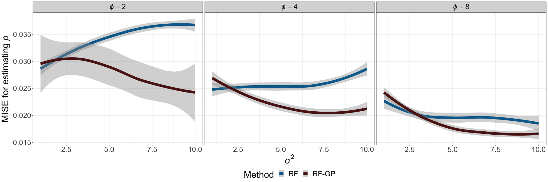
Figure 1: MISE for estimates of the mean function $p\left(\cdot\right)$ in (4) as a function of spatial signal strength $\sigma^{2}$ for different values of $\phi$.

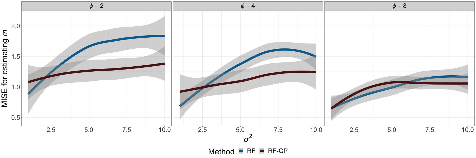
Figure 2: MISE for estimates of the non-linear covariate effect $m\left(\cdot\right)$ in (3) as a function of spatial signal strength $\sigma^{2}$ for different values of $\phi$.

5.1.2 Prediction performance

Next, we focus on prediction, which is often the primary focus of spatial inference procedure. We compare the prediction performance of all four methods with respect to the Relative Mean Squared Error (MSE) for the test data. As the name suggests, MSE computes the average squared difference between the true response and the predicted outcome. Here, we measure how closely the competing methods predict the true probabilities of the Bernoulli process generating the observed outcomes in the test data, i.e. $\mathbb{E}\left(Y|X,s\right)$. We note that as the spatial signal strength $(\sigma^{2})$ increases, the variance of the response increases. Hence, in order to make the performance metric comparable across different $\sigma^{2}$ values, we use Relative MSE, which accounts for the variance of the response as follows:

$$\mathrm{Relative\>MSE}\left(\{\hat{p}_{1},\hat{p}_{2},\ldots,\hat{p}_{n_{T}}\},\{p_{1},p_{2},\ldots,p_{n_{T}}\}\right)=\frac{\sum_{j=1}^{n_{T}}\left(\hat{p}_{j}-p_{j}\right)^{2}}{\mathrm{var}\left(\{p_{1},p_{2},\ldots,p_{n_{T}}\}\right)},$$

where $n_{T}$ is the number for samples in the test data, and $\{\hat{p}_{1},\hat{p}_{2},\ldots,\hat{p}_{n_{T}}\}$ are the prediction of the true probabilities $\{p_{1},p_{2},\ldots,p_{n_{T}}\}$. Here we note that, in the simulation setup, we have complete knowledge of true probabilities generating the response in the test data, hence we make use of MSE for comparing the prediction performances. In analysis of real data where we do not have the knowledge of true probabilities we use the outcomes in the test data to evaluate binary data specific prediction metrics like the mis-classification error or the Kullback-Leibler divergence.

The prediction results are presented in Figure 3. RF-GP produces better or comparable prediction performance to all its competitors across all scenarios. The classical RF, unlike the other three methods under consideration, doesn’t use any spatial information. This results in huge disparity between RF and RF-GP, which only increases as the spatial signal strength increases. RF-Loc, though performs better than RF, follows a similar pattern. In low spatial signal strength, RF-Loc outperforms RF-Sp, whereas RF-Sp outperforms RF-Loc for moderate spatial signal strength. This is because RF-sp adds several ($O(n)$) spatial covariates which can drown out the effect of the true covariates. This negatively impacts its performance at scenarios with low spatial correlation where the true covariate effect dominates the signal. RF-GP combines the best of both worlds and outperforms both RF-Loc and RF-Sp significantly for both low and moderate spatial signal strength. Even at very low (covariate) signal to (spatial) noise ratio, i.e., when $\sigma^{2}$ is large, RF-GP produces comparable results to that of RF-Sp. As far as spatial decay is concerned, the difference between RF-GP and the rest of the methods are highest, when $\phi$ is small, i.e. the data is very highly correlated. RF-GP can also account for weak correlation in the data and outperforms the rest of the methods even when $\phi$ is very high, albeit by smaller margins.

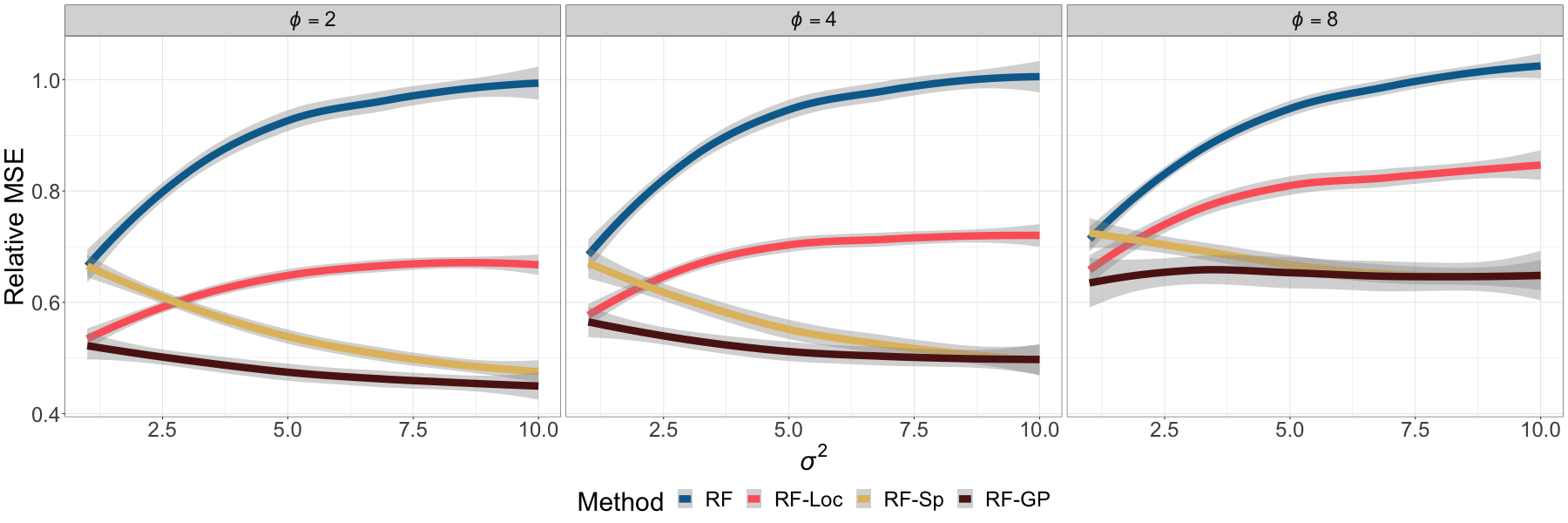
Figure 3: Relative MSE for spatial predictions of $\mathbb{E}\left(Y|X,w\right)$ in (3) as a function of spatial signal strength $\sigma^{2}$ for different values of $\phi$.

5.2 Soil type prediction

We demonstrate the utility of RF-GP to improve classification of spatial binary data in a real world application. We study the spatial pattern of soil types in the Meuse data (available in the sp package in R). This dataset contains information on soil type, heavy metal concentration, and landscape variables at 155 locations, spread over approximately $15\textrm{m}\times 15\textrm{m}$ area in the flood plain of the river Meuse in Netherlands. We consider the presence and absence data of the dominant soil type (Type 1) in the area. Soil type is primarily determined by its distance from the river. Additionally, surface water occurrence may also play a role in soil forming process (Pekel et al.,, 2016). Following Hengl et al., (2018), we consider both distance from river Meuse and surface water occurrence as the covariates for predicting the presence of the dominant soil type. In Figure 4, we demonstrate example of a test and training data split ($20\%-80\%$), whereas the background demonstrates different discretised levels of distances from river Meuse. A spatial structure is evident in the binary response, which seems to be correlated with distance from river, a highly spatial covariate by definition. Now we investigate if there is any spatial correlation in the binary response beyond the effect of the spatial covariates. We perform prediction with classical RF, and compare its performance with RF-GP, which unlike the former, explicitly models the spatial correlation. In Figure 4, we observe that RF prediction fail to account for spatial trends beyond covariate effects whereas RF-GP successfully accounts for this.

To highlight this, we focus on two pairs of locations in the RF prediction in Figure 4. For the pair of locations in the blue oval near the river, RF predicts it is highly probable that the dominant soil type will be present in these locations, whereas it is absent in the test data. Since RF only makes use of covariate information, this is consistent with the training data, where the dominant soil type is present near the river. As RF doesn’t take into consideration spatial information, it fails to account for the fact that in a number of nearby locations, albeit a little further from the river, the dominant soil type is absent. RF-GP accounts for this information, and correctly predicts a much lower probability of observing the specific soil type in these locations. For the pair of points in yellow oval in RF prediction in Figure 4, we observe an opposite scenario where RF predicts low-probability of the dominant soil type as these locations are further away from the river, but RF-GP accurately estimates a high probability of the soil type by leveraging spatial correlations. This indicates that incorporating the spatial information in RF might improve the prediction performance.

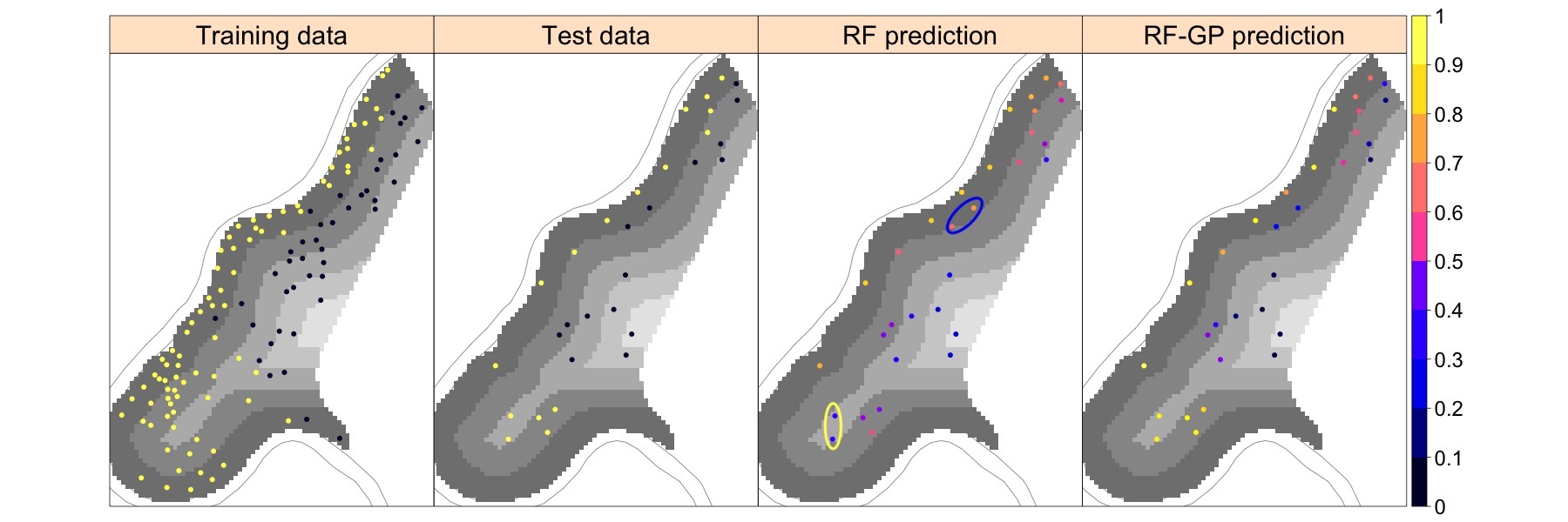
Figure 4: Plot of training and test data alongside prediction from classical RF and RF-GP overlaid on discretised distances from river. The blue and yellow oval in RF prediction points out two pairs of points, which classical RF mis-classifies due to not accounting for spatial correlation beyond covariate effect. RF-GP explicitly models this spatial correlation and correctly classifies these pairs of points.

In order to ensure that this is not an artifact of this specific train-test split, we consider 100 random $20\%-80\%$ test-train split of the data. We perform prediction with classical RF, RF-Sp, RF-Loc, and RF-GP. Here we do not have access to the probabilities corresponding to the underyling process generating the test data response, hence we measure the prediction performance based on test mis-classification error. This computes the fraction of mis-classification in binary prediction problems, and has the same functional form as that of MSE. In Figure 5, we plot the histogram of the mis-classification error and we report the median mis-classification rate corresponding to each method in Table 1. As expected, classical RF, which doesn’t use any spatial information beyond the covariate effects, has the highest mis-classification error. Both RF-Loc and RF-sp, which incorporates spatial information through additional covariates, perform similarly to each other, and improve over naïve RF. RF-GP, with its parsimonious modelling of spatial information performs the best among the all the competing algorithms. RF-GP offers a $33\%$ improvement from its nearest competitors (RF-Sp and RF-Loc) both in terms of the median classification error. It also has the thinnest tail (Figure 5), i.e., the lowest probability of producing extreme mis-classification rates due to sampling variability in the training data.

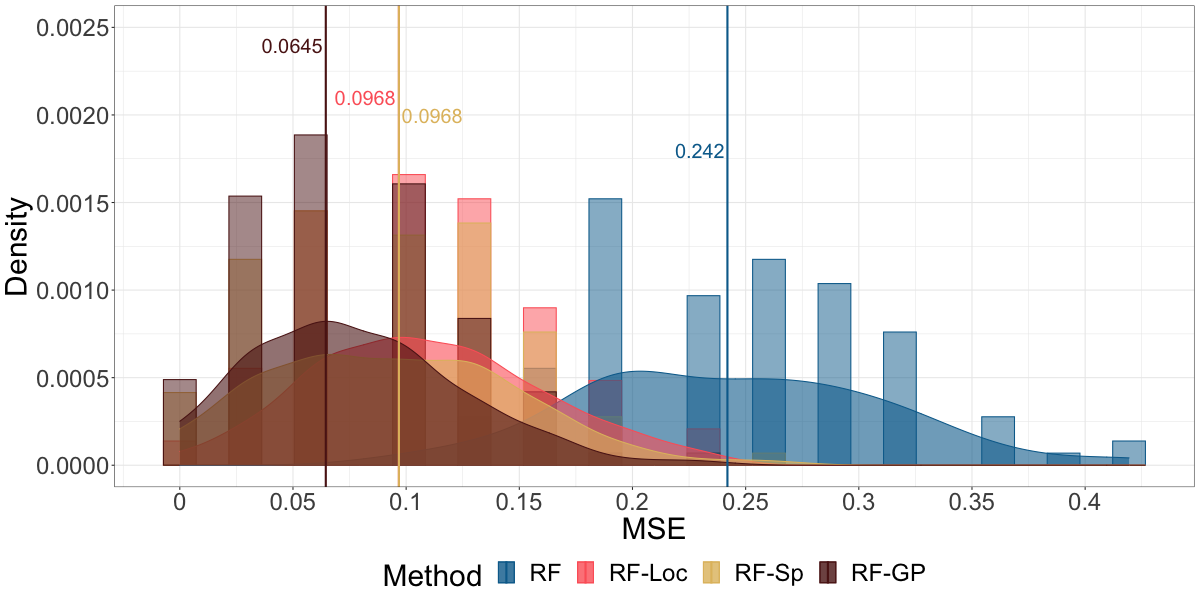
Figure 5: Histogram of the mis-classification errors correponding to RF, RF-Loc, RF-Sp, and RF-GP in Meuse data. The color-coordinated vertical lines indicates the median values corresponding to different methods.

	RF	RF-Loc	RF-Sp	RF-GP
Mis-classification error	$0.242$	$0.0968$	$0.0968$	$0.0645$

Table 1: Median values of the mis-classification error for the competing methods.

6 Discussion

We propose RF-GP, a novel approach for using Random Forests for binary spatially dependent data directly within the traditional generalized mixed model framework which accounts for spatial correlation via Gaussian Processes. We observe that Gini impurity measure used in classical RF for binary data can be re-imagined as an OLS loss with the binary outcome. We can then generalize the OLS loss to GLS loss to account for the spatial structure in the data when building the regression trees (Saha et al., 2021a, ) for estimating the mean function. Subsequently, we present a novel link-inversion method that allows estimating the covariate effect via a simple probit GLMM as well as facilitates predictions at new locations using scalable algorithms. Our approach is both a generalization of the classical RF and a generalization of the traditional spatial generalized linear mixed models, thereby retaining all advantages of the GP-based mixed model framework for estimation and prediction using GP.

Existing RF methods for spatial binary data depart the generalized mixed model framework and incorporate the spatial information as additional covariates, which is a hindrance in recovering the true covariate effect. Working directly within the traditional generalized mixed model setup allows us to bypass this problem. We also circumvent adding too many spatial covariates which can lead to curse of dimensionality and poor empirical performance. Simulation results and application in real data indicate that RF-GP compares quite favorably to that of classical RF and other state-of-the-art spatially informed RF methods.

There is very little theoretical support for existing RF methods for binary spatial data. We establish $\mathbb{L}_{2}$ consistency of RF-GP for estimation of both the mean function and the covariate effect. Traditional theoretical analysis of $\mathbb{L}_{2}$ consistency for RF (Scornet et al.,, 2015; Saha et al., 2021a, ) depends heavily on additivity of the mean function. We relax this assumption as it does not hold for generalized mixed effect models with nonlinear link functions. This result can be of independent interest for studying consistency of random forests in other settings where the mean function is not additive.

For large data, choosing the parameters for working correlation matrix and binary prediction in RF-GP through cross-validation can be computationally challenging. Future work will explore ways of scaling the parameter estimation. Additionally, extending RF-GP for categorical outcomes with more than two categories and for other types of non-Gaussian spatial data within the generalized mixed model framework is of potential future interest.

S1 Time-series GMEM with autoregressive error

We also study property of RF-GP for binary time-series with an autoregressive covariance structure for the temporal random effects. Assuming a lag or order $q$, i.e., $\mathrm{AR}(q)$ structure, the hierarchical model can be expressed as

$$Y_{i} \overset{ind}{\sim}\mbox{Bernoulli}(h(m(X_{i})+w_{i}))$$ (S1)

$$w_{i} =a_{1}w_{i-1}+a_{2}w_{i-2}+\ldots+a_{q}w_{i-q}+\eta_{i}$$

Here $\eta_{i}$ is a realization of a white noise process at time $i$. It can be shown that $w_{i}$ is a $\beta$-mixing process (Mokkadem,, 1988). When fitting RF-GP, we use a working covariance matrix also having an autoregressive structure (as justified in Section S2.1). The lag order for the working covariance matrix need not match auto-regression lag assumed for the data generation, and for all choices of lag the working covariance matrix satisfies the regularity assumptions 2. Hence, we immediately have the following result:

Corollary S1.1.

Consider a binary time series (S1) in a generalized mixed model setup with probit or logit link and with temporal random effects distributed as a sub-Gaussian stable $\mathrm{AR}(q)$ process. Let Q denote a diagonally dominant working precision matrix from a stationary $\mathrm{AR}(q^{\prime})$ process. Then RF-GP using Q produces an $\mathbb{L}_{2}$ consistent estimate of $\mathbb{E}(Y|X)$ and $m(X)$.

S2 Implementation of RF-GP

S2.1 Working correlation matrix

The estimate of the mean function $p(\cdot)$ in Section 3.1 requires a suitable working covariance matrix $\textbf{Q}^{-1}$ that adequately captures the spatial dependence in the data. The finite sample performance of GLS estimators depends on how closely the working covariance matrix approximates the population covariance matrix $\mbox{\boldmath$\Sigma$}=Cov(\mathbf{Y}\,|\,\textbf{X})$. In RF-GLS with continuous outcome, due to the linear relationship between the outcome and the spatial random effects, the population covariance of the outcome is the sum of the covariance of w and the noise covariance. In case of binary outcome with a non-linear link $h$, there is no closed form expression of the marginal population covariance matrix $\Sigma$ of $\mathbf{Y}\,|\,\textbf{X}$, even when w has a structured covariance matrix C.

For non-Gaussian data there is a long-established history of using working covariance matrices in generalized estimating equations (Liang and Zeger,, 1986). We follow the conventional GLM approach in considering working covariance matrices of the form

$$\textbf{Q}^{-1}=\sigma_{w}^{2}\mathbf{V}^{1/2}\textbf{R}(\mbox{\boldmath$\zeta$})\mathbf{V}^{1/2}$$ (S2)

where $\mathbf{V}$ is a diagonal matrix with entries $a(p(X_{i}))$, $a(\cdot)$ being a working variance function, and R is a working correlation matrix parameterized by $\zeta$, capturing the spatial dependence. Common choices of $v(\cdot)$ can be the Bernoulli ($a(p)=p(1-p)$) or Gaussian ($a\equiv 1$) working variance functions (McCullagh and Nelder,, 2019). We use the latter as other choices will involve the i=unknown mean function $p$. We show in Section 4 that this choice of the variance function along the choice of the correlation matrix described below leads to consistent estimates for our algorithm.

For the working spatial correlation matrix $\textbf{R}(\mbox{\boldmath$\zeta$})$, based on a first order Taylor series approximation

$$Cov(Y_{i},Y_{j}\,|\,\textbf{X}) =E(Cov(Y_{i},Y_{j}\,|\,\textbf{X},\textbf{w})\,|\,\textbf{X})+Cov(E(Y_{i}\,|\,\textbf{X},\textbf{w}),E(Y_{j}\,|\,\textbf{X},\textbf{w})\,|\,\textbf{X})$$

$$=0+Cov(h(m(X_{i})+w(s_{i})),h(m(X_{j})+w(s_{j}))\,|\,\textbf{X})$$

$$\approx Cov(h(m(X_{i}))+w(s_{i})h^{\prime}(m(X_{i})),h(m(X_{j}))+w(s_{j})h^{\prime}(m(X_{j}))\,|\,\textbf{X})$$

$$=h^{\prime}(m(X_{i}))h^{\prime}(m(X_{j}))C_{ij},$$

we see that $Corr(Y_{i},Y_{j}\,|\,\textbf{X})\propto C_{ij}$. Hence, we choose $\textbf{R}(\mbox{\boldmath$\zeta$})$ from the same covariance family $C$ which specifies the GP distribution of the spatial random effects w. However, we allow the parameter for $\zeta$ for R to be different from the parameters $\theta$ of the GP covariance function $C$ generating the spatial random effects. We use the popular Nearest Neighbor GP (NNGP) approximation of the working spatial matrix $\textbf{R}(\mbox{\boldmath$\zeta$})$. Theoretical justification of using NNGP working covariance function is provided in Proposition 4.1. Subsequent to choosing the functional form of the working precision matrix Q, we estimate the hyper-parameters specifying it using cross-validation, detailed afterwards.

S2.2 Estimation details

For the estimation of the mean function in RF-GP, which uses RF-GLS, we fix the number of trees in the to be $n_{tree}=100$; the minimum cardinality of leaf nodes to be $t_{c}=20$ and number of features to be considered at each split to be $M_{try}=\min\{1,\left[\frac{D}{3}\right]\}$, where $D$ is number of features in the covariate space. We assume the exponential covariance function for the spatial random effects $w$. Hence, as explained in Section S2.1, we also use the same covariance function form to define the working correlation matrix in S2.1. We need to estimate two sets of spatial parameters for fitting RF-GP. The first one being the spatial decay parameter of the exponential covariance function in the working correlation matrix $\mathbf{R}$, denoted as $\zeta$. The other one is the set of spatial parameters corresponding to the spatial process $w$, needed for estimation of the fixed effect and predictions. This is given by $\bm{\theta}=\left(\sigma^{2},\phi\right)$ where $\sigma^{2}$ is the variance and $\phi$ is the spatial decay. We estimate the parameters by 2-fold cross-validation with respect to the mis-classification error. We perform the cross-validation through a grid search with $\mbox{\boldmath$\zeta$}\in\left\{1,4,7,10,\infty\right\}$, $\sigma^{2}\in\left\{1,2.5,5,7.5,\ldots,25\right\}$, and $\phi=\frac{3}{\sqrt{2}f}$, where $f\in\left\{0.05,0.25,0.5,0.75,0.95\right\}$. Here we note that the first part of RF-GP, i.e., estimating the mean function using RF-GLS depends only on $\zeta$. We incorporate $\mbox{\boldmath$\zeta$}=\infty$ in the cross-validation parameter set as it corresponds to an identity working covariance matrix, in which case, the mean function estimation with RF-GLS becomes equivalent to the classical RF. This choice is included to account for possible absence of spatial correlation structure in the data and in practice implemented by using a very large $\mbox{\boldmath$\zeta$}(=1000)$. The methods were implemented in R. For model fitting, we used RandomForestsGLS (Saha et al., 2021b, ) to implement RF-GP and randomForest (Liaw and Wiener,, 2002) to implement the remaining methods. We used probit-NNGP (Saha et al., 2022b, ) implemented BRISC (Saha and Datta,, 2022) for binary prediction.

Estimating the covariate effect using link inversion (7) requires the mean estimates $\widehat{p(\textbf{x})}=\widehat{\mathbb{E}\left(Y|X=\mathbf{x}\right)}$ to lie in $\left(0,1\right)$. Neither RF nor RF-GP estimates are guaranteed to lie in $\left(0,1\right)$. For small imbalanced data, RF mean estimate at a covariate value can coincide with $0$ or $1$, depending on the predominant class. RF-GP estimates of the mean function are obtained using RF-GLS. Being a GLS estimate, it is not guaranteed to lie in $\left(0,1\right)$ although it is uniformly bounded (Lemma 4.4). For mean estimation, we truncate the original estimate at $[0,1]$. For link inversion, we interpolate the estimates to $(0,1)$ exploiting the assumed regularity of the covariate effect $m\left(\cdot\right)$. If the mean estimate at a covariate value lies outside $(0,1)$, we first generate points x uniformly in the covariate space and obtain $\widehat{p}(\textbf{x})$ from the RF-GLS estimate. Next we train any statistical interpolator $model$ with only the $\widehat{p}(\textbf{x})$’s which lie in $(0,1)$ and the corresponding x’s. Then for x’s for which $\widehat{p}(x)$ lie outside $(0,1)$, we replace $\widehat{p}(x)$ with the predicted value from the interpolator. We use classical RF for this interpolation as it preserves the range of the outcomes in the training data, although any other interpolator with the same property can also be used.

S3 Proofs

S3.1 Proof of Theorem 3.1

Proof.

In order to prove this, we begin with the following proposition showing that the Gini node impurity measure is a constant multiplier of the node variance.

Proposition S3.1.

For given data $(Y_{i},X_{i})\in\{0,1\}\times\mathbb{R}^{D};i=1,2,\cdots,n$, and a node $\mathcal{T}\subseteq\mathbb{R}^{D}$

$$\frac{1}{2}I(\mathcal{T})=\frac{1}{\sum_{i=1}^{n}\mathds{1}_{\{X_{i}\in\mathcal{T}\}}}\sum_{i=1}^{n}\mathds{1}_{\{X_{i}\in\mathcal{T}\}}(Y_{i}-\bar{Y}^{(\mathcal{T})})^{2},$$ (S3)

where, $\bar{Y}^{(\mathcal{T})}=\frac{1}{\sum_{i=1}^{n}\mathds{1}_{\{X_{i}\in\mathcal{T}\}}}\sum_{i=1}^{n}\mathds{1}_{\{X_{i}\in\mathcal{T}\}}Y_{i}$.

Proof.

We begin our proof with the following observation:

$$\bar{Y}^{(\mathcal{T})} =\frac{1}{\sum_{i=1}^{n}\mathds{1}_{\{X_{i}\in\mathcal{T}\}}}\sum_{i=1}^{n}\mathds{1}_{\{X_{i}\in\mathcal{T}\}}Y_{i}$$

$$=\frac{\sum_{i=1}^{n}\mathds{1}_{\{Y_{i}=1\}\cap\{X_{i}\in\mathcal{T}\}}}{\sum_{i=1}^{n}\mathds{1}_{\{X_{i}\in\mathcal{T}\}}}$$

$$=p^{({\mathcal{T}})},$$

where $p^{(\mathcal{T})}$ is defined in (2b) and the second inequality follows from the binary nature of $Y$. Substituting $p^{({\mathcal{T}})}$ for $\bar{Y}^{(\mathcal{T})}$ in (S3) we have,

$$\frac{1}{\sum_{i=1}^{n}\mathds{1}_{\{X_{i}\in\mathcal{T}\}}}\sum_{i=1}^{n}\mathds{1}_{\{X_{i}\in\mathcal{T}\}}(Y_{i}-\bar{Y}^{(\mathcal{T})})^{2}$$

$$= \frac{1}{\sum_{i=1}^{n}\mathds{1}_{\{X_{i}\in\mathcal{T}\}}}\sum_{i=1}^{n}\mathds{1}_{\{X_{i}\in\mathcal{T}\}}(Y_{i}-p^{({\mathcal{T}})})^{2}$$

$$= \frac{1}{\sum_{i=1}^{n}\mathds{1}_{\{X_{i}\in\mathcal{T}\}}}\left[\sum_{i=1}^{n}\mathds{1}_{\{Y_{i}=1\}\cap\{X_{i}\in\mathcal{T}\}}(1-p^{({\mathcal{T}})})^{2}+\mathds{1}_{\{Y_{i}=0\}\cap\{X_{i}\in\mathcal{T}\}}(-p^{({\mathcal{T}})})^{2}\right]$$

$$= \left(1-p^{({\mathcal{T}})}\right)^{2}\frac{\sum_{i=1}^{n}\mathds{1}_{\{Y_{i}=1\}\cap\{X_{i}\in\mathcal{T}\}}}{\sum_{i=1}^{n}\mathds{1}_{\{X_{i}\in\mathcal{T}\}}}+(-p^{({\mathcal{T}})})^{2}\left(1-\frac{\sum_{i=1}^{n}\mathds{1}_{\{Y_{i}=1\}\cap\{X_{i}\in\mathcal{T}\}}}{\sum_{i=1}^{n}\mathds{1}_{\{X_{i}\in\mathcal{T}\}}}\right)$$

$$=p^{({\mathcal{T}})}\left(1-p^{({\mathcal{T}})}\right)^{2}+p^{{(T)}^{2}}\left(1-p^{({\mathcal{T}})}\right)$$

$$=p^{({\mathcal{T}})}(1-p^{({\mathcal{T}})})$$

$$=\frac{1}{2}I(\mathcal{T})$$

where, the last equality follows from (2a). This completes the proof of the Proposition S3.1. ∎

Substituting the value of $I(\mathcal{T}),I(\mathcal{L})$ and $I(\mathcal{R})$ from Proposition S3.1 in (2c), we have,

$$\Delta_{n}^{CT}((d,c))=\frac{2}{\sum_{i=1}^{n}\mathds{1}_{\{X_{i}\in\mathcal{T}\}}}\sum_{i=1}^{n}\mathds{1}_{\{X_{i}\in\mathcal{T}\}}(Y_{i}-\bar{Y}^{(\mathcal{T})})^{2}-\frac{\sum_{i=1}^{n}\mathds{1}_{\{X_{i}\in\mathcal{L}\}}}{\sum_{i=1}^{n}\mathds{1}_{\{X_{i}\in\mathcal{T}\}}}\frac{2}{\sum_{i=1}^{n}\mathds{1}_{\{X_{i}\in\mathcal{L}\}}}\sum_{i=1}^{n}\mathds{1}_{\{X_{i}\in\mathcal{T}\}}(Y_{i}-\bar{Y}^{(\mathcal{L})})^{2}-\frac{\sum_{i=1}^{n}\mathds{1}_{\{X_{i}\in\mathcal{R}\}}}{\sum_{i=1}^{n}\mathds{1}_{\{X_{i}\in\mathcal{T}\}}}\frac{2}{\sum_{i=1}^{n}\mathds{1}_{\{X_{i}\in\mathcal{R}\}}}\sum_{i=1}^{n}\mathds{1}_{\{X_{i}\in\mathcal{R}\}}(Y_{i}-\bar{Y}^{(\mathcal{R})})^{2}=\frac{2}{\sum_{i=1}^{n}\mathds{1}_{\{X_{i}\in\mathcal{T}\}}}\left[\sum_{i=1}^{n}\mathds{1}_{\{X_{i}\in\mathcal{T}\}}(Y_{i}-\bar{Y}^{(\mathcal{T})})^{2}-\sum_{i=1}^{n}\mathds{1}_{\{X_{i}\in\mathcal{L}\}}(Y_{i}-\bar{Y}^{(\mathcal{L})})^{2}-\sum_{i=1}^{n}\mathds{1}_{\{X_{i}\in\mathcal{R}\}}(Y_{i}-\bar{Y}^{(\mathcal{R})})^{2}\right]=2v_{n}^{RT}((d,c))$$ (S4)

This completes the proof of the Theorem 3.1. ∎

S3.2 Proof of Proposition 3.1

Proof.

Since, $1>h>0$, and $f(t)\geqslant 0$, we have

$$0<\int h(z_{0}+t)d\mathbb{F}_{w}(t)=g_{h,\mathbb{F}_{w}}(z_{0})<\int_{\mathbb{R}}d\mathbb{F}_{w}(t)=1.$$

Additionally, for any $z_{1}>z_{0}$ we have

$$g_{h,\mathbb{F}_{w}}(z_{1})-g_{h,\mathbb{F}_{w}}(z_{0})=\int\left(h(z_{1}+t)-h(z_{0}+t)\right)d\mathbb{F}_{w}(t)>0$$

as $h$ is strictly increasing. Hence $g_{h,\mathbb{F}_{w}}$ is strictly increasing. Letting $I$ be the support of $m(\cdot)$ and $im(I)$ be its image after applying $m$, there exists an inverse map $g_{h,\mathbb{F}_{w}}^{+}:im(I)\mapsto I$, such that $g_{h,\mathbb{F}_{w}}^{+}(g_{h,\mathbb{F}_{w}}(z_{0}))=z_{0},\forall z_{0}\in I$. ∎

S3.3 Proofs for results of Section 4.4

Proof of Lemma 4.1.

From Assumption 1.b, $\{X_{i}\}$ is in i.i.d. process. 1.d dictates that $\{W_{i}\}$ is a $\beta$-mixing process, independent of $\{X_{i}\}$. Following the proof of Lemma A.1. in Saha et al., 2021a , $\{X_{i},W_{i}\}$ is a $\beta$-mixing process. By construction in (14), the i.i.d. process $\{U_{i}\}$ is independent of the $\beta$-mixing process $\{X_{i},W_{i}\}$. Hence a second application of the aforementioned result proves that $\{U_{i},X_{i},W_{i}\}$ is $\beta$-mixing process. We can similarly prove that for any finite $j\neq j^{\prime}<K\in\mathbb{N}$, $\{U_{i-j^{\prime}},X_{i-j^{\prime}},X_{i-j},W_{i-j^{\prime}}\}$ is a $\beta$-mixing process. ∎

Proof of Lemma 4.2.

We note that the split criterion (6b) is a function of expressions of the form $\textbf{Z}^{\top}\textbf{Q}\textbf{Y}$, $\textbf{Z}^{\top}\textbf{Q}\textbf{Z}$, $\textbf{Y}^{\top}\textbf{Q}\textbf{Y}$. Each entry of all these expressions is a quadratic form in Q.

For any two $n\times 1$ vectors u and v, under Assumption 2.a, we can write a quadratic form of Q as

$$\textbf{u}^{\top}\textbf{Q}\textbf{v} =\gamma\sum_{i}u_{i}v_{i}+\sum_{j\neq j^{\prime}=0}^{q}\rho_{j}\rho_{j^{\prime}}\sum_{i}u_{i-j}v_{i-j^{\prime}}+\sum_{i\in\mathcal{A}}\sum_{i^{\prime}\in\mathcal{A}^{\prime}}\tilde{\gamma}_{i,i^{\prime}}u_{i}v_{i^{\prime}},$$ (S5)

where $\gamma=\|\mbox{\boldmath$\rho$}\|_{2}^{2}$, ${\mathcal{A}},{\mathcal{A}}^{\prime}\subset\{1,2,\cdots,n\}$ with $|{\mathcal{A}}|,|{\mathcal{A}}^{\prime}|\leq 2q$, $\tilde{\gamma}_{i,i^{\prime}}$’s are fixed (independent of $n$) functions of L and $\rho$ in (11), and $u_{i}$, $v_{i}$ for $i\leq 0$ are defined to be zero.

First, we focus on the asymptotic limit of the node representative of the leaf-nodes given by (6c). We show that, alike the continuous case, in the binary case too, the GLS-loss based node representative converges to the mean of the response, conditional on the covariate belonging the specific leaf node. We will show that for a data-independent, pre-fixed tree with leaf nodes denoted by ${\mathcal{B}}_{1},{\mathcal{B}}_{2},\ldots,{\mathcal{B}}_{K}$, we have

$$\bm{\hat{\beta}}_{{l}}\overset{a.s.}{\to}\mathbb{E}(Y|X\in\mathcal{B}_{{l}})\text{ as $n\to\infty$}\mbox{ for }l=1,\ldots,K.$$ (S6)

where, $\bm{\hat{\beta}}_{{l}}$ corresponds to the estimate (6c) corresponding to node ${\mathcal{B}}_{l},l=1,2,\cdots,K$.

As $\bm{\hat{\beta}}=\left(\mathbf{Z}^{\top}\textbf{Q}\mathbf{Z}\right)^{-1}\mathbf{Z}^{\top}\textbf{Q}\mathbf{Y}$, we consider the asymptotic limits of $\left(\frac{1}{n}\mathbf{Z}^{\top}\textbf{Q}\mathbf{Z}\right)^{-1}$ and $\frac{1}{n}\mathbf{Z}^{\top}\textbf{Q}\mathbf{Y}$ separately. We first consider the asymptotic limit of $\frac{1}{n}\mathbf{Z}^{\top}\textbf{Q}\mathbf{Y}$. Following S5 we have:

$$\frac{1}{n}(\mathbf{Z}^{\top}\textbf{Q}\mathbf{Y})_{l} =\frac{1}{n}\left[\gamma\sum_{i}\mathbf{Z}_{i,l}Y_{i}+\sum_{j\neq j^{\prime}=0}^{q}\rho_{j}\rho_{j^{\prime}}\sum_{i}\mathbf{Z}_{i-j,l}Y_{i-j^{\prime}}+O_{b}(1)\right]$$ (S7)

where $O_{b}(1)$ denotes a sequence of random variances which are uniformly bounded.

1. Asymptotic limit of $\frac{1}{n}\sum_{i}\mathbf{Z}_{i,l}Y_{i}$ : By lemma 4.1, $\{U_{i},X_{i},w_{i}\}$ is a $\beta$-mixing process and $\mathbf{Z}_{i,l}Y_{i}$ is a function of $(U_{i},X_{i},w_{i})$, as as $\mathbf{Z}_{i,l}=\mathds{1}\{X_{i}\in\mathcal{B}_{l}\}$ and $Y_{i}=\mathds{1}\{U_{i}\leqslant h(m(X_{i})+w_{i})\}$. We use the Uniform Law of Large Number (ULLN) for $\beta$-mixing process in Theorem 1 from Nobel and Dembo, (1993), which shows that if a class of functions with uniformly integrable envelop satisfies uniform law of averages with respect to an i.i.d. process, then it also satisfies the uniform law of averages for stationary, $\beta$-mixing stochastic process with identical marginal distribution. We consider the class of function with a singleton function $(U_{i},X_{i},w_{i})\mapsto\mathbf{Z}_{i,l}Y_{i}$. Since $\mathbf{Z}_{i,l}Y_{i}\leqslant\mathbf{Z}_{i,l}\leq 1$ , which is uniformly integrable, we have that strong law holds for $\mathbf{Z}_{i,l}Y_{i}$, i.e.

   $$\lim_{n\to\infty}\frac{1}{n}\mathbf{Z}_{i,l}Y_{i}\overset{a.s.}{=}\mathbb{E}\left(\mathbf{Z}_{1,l}Y_{1}\right)=\mathbb{E}\left(Y|X\in\mathcal{B}_{l}\right)Vol(\mathcal{B}_{l})$$ (S8)

2. Asymptotic limit of $\frac{1}{n}\sum_{i}\mathbf{Z}_{i-j,l}Y_{i-j^{\prime}}$ : For $j\neq j^{\prime}$, by Lemma 4.1, $\{U_{i-j^{\prime}},X_{i-j^{\prime}},X_{i-j},W_{i-j^{\prime}}\}$ is a $\beta$-mixing process and $\mathbf{Z}_{i-j,l}Y_{i-j^{\prime}}$ is a function of $(U_{i-j^{\prime}},X_{i-j^{\prime}},X_{i-j},W_{i-j^{\prime}})$ as shown before. Since $\mathbf{Z}_{i-j,l}Y_{i-j^{\prime}}\leqslant\mathbf{Z}_{i-j,l}$ with $\mathbf{Z}_{i-j,l}$ uniformly integrable, applying Theorem 1 from Nobel and Dembo, (1993) with class of function containing the single function $(U_{i-j^{\prime}},X_{i-j^{\prime}},X_{i-j},W_{i-j^{\prime}})\mapsto\mathbf{Z}_{i-j,l}Y_{i-j^{\prime}}$, we have

   $$\lim_{n\to\infty}\frac{1}{n}\sum_{i}\mathbf{Z}_{i-j,l}Y_{i-j^{\prime}}\overset{a.s.}{=}\mathbb{E}\left(\mathbf{Z}_{2q-j,l}Y_{2q-j^{\prime}}\right)=\mathbb{E}\left(Y\right)Vol(\mathcal{B}_{l}),$$ (S9)

   where, the last equality follows from the independence of $\mathbf{Z}_{i-j,l}$ and $Y_{i-j^{\prime}}$ for $j\neq j^{\prime}$.

Combining (S8) and (S9), we have:

$$\lim_{n\to\infty}\frac{1}{n}(\mathbf{Z}^{\top}\textbf{Q}\mathbf{Y})_{l}\overset{a.s.}{=}\gamma\mathbb{E}(Y\mathds{I}(X\in\mathcal{B}_{l}))+Vol(\mathcal{B}_{l})\mathbb{E}(Y)\sum_{j\neq j^{\prime}=0}^{q}\rho_{j}\rho_{j^{\prime}}.$$ (S10)

This is the same limit as that for continuous $Y$ in Saha et al., 2021a . For prefixed data-independent partition, $\left(\mathbf{Z}^{\top}\textbf{Q}\mathbf{Z}\right)^{-1}$ is not affected by distribution of the outcome $Y$. Hence, this quantity also asymptotes to the same limit as in the continuous case.

$$\left(\lim_{n\to\infty}\frac{1}{n}\mathbf{Z}^{\top}\textbf{Q}\mathbf{Z}\right)^{-1} =\gamma^{-1}\left[diag(\mathbf{b}^{-1})-\frac{\left(\sum_{j\neq j^{\prime}=0}^{q}\rho_{j}\rho_{j^{\prime}}\right)}{\gamma+\sum_{j\neq j^{\prime}=0}^{q}\rho_{j}\rho_{j^{\prime}}}\mathbf{1}\mathbf{1}^{\top}\right].$$ (S11)

where $\mathbf{b}$ is the diagonal of the volume of the leaf nodes.

Multiplying (S11) and (S10) and simplifying, we have (S6). The GLS cost function corresponding to membership Z is $\left(\mathbf{Y}-\mathbf{Z}\bm{\hat{\beta}}(\mathbf{Z})\right)^{\top}\textbf{Q}\left(\mathbf{Y}-\mathbf{Z}\bm{\hat{\beta}}(\mathbf{Z})\right)=\mathbf{Y}^{\top}\textbf{Q}\mathbf{Y}-\mathbf{Y}^{\top}\textbf{Q}\mathbf{Z}\bm{\hat{\beta}}(\mathbf{Z})$. Since $v_{n,\mathbf{Q}}^{DART}((d,c))$ in (6b) is a difference of cost function corresponding to the membership matrix Z before and after the split, the $\mathbf{Y}^{\top}\textbf{Q}\mathbf{Y}$ component cancels out and it is enough to focus on asymptotic limit of differences of $\mathbf{Y}^{\top}\textbf{Q}\mathbf{Z}\bm{\hat{\beta}}(\mathbf{Z})$. Since we have already shown the asymptotic limits of $\frac{1}{n}(\mathbf{Z}^{\top}\textbf{Q}\mathbf{Y})_{l}$ and $\bm{\hat{\beta}}$ to be identical for both the continuous and binary outcome, following Saha et al., 2021a , we have that the asymptotic limit of $v_{n,\mathbf{Q}}^{DART}((d,c))$ in (6b) will coincide for both binary and continuous outcome, i.e. $\lim_{n\to\infty}v_{n,\mathbf{Q}}^{DART}((d,c))\overset{a.s.}{=}\Delta_{\textbf{Q}}^{*}((d,c))$. ∎

Proof of Lemma 4.3.

From Section 3.2 we have $p(X_{i}):=\mathbb{E}(Y_{i}|X_{i})=\mathbb{E}_{w}h(m(X_{i})+w(s_{i}))=g_{h,\mathbb{F}_{w}}(X_{i})$. As $m(\cdot)$ is continuous, and image of $h(\cdot)$ lies in $[0,1]$, $p(\cdot)$ is continuous by the dominated convergence theorem.

From Lemma 4.2 we have

$$\Delta_{\textbf{Q}}^{*}((d,c))= \gamma(\textbf{Q})Vol(\mathcal{A})\Big{[}\mathbb{V}(Y|\mathbf{X}\in\mathcal{A})-\mathbb{P}(\mathbf{X}\in\mathcal{A}^{R}|\mathbf{X}\in\mathcal{A})\mathbb{V}(Y|\mathbf{X}\in\mathcal{A}^{R})$$

$$-\mathbb{P}(\mathbf{X}\in\mathcal{A}^{L}|\mathbf{X}\in\mathcal{A})\mathbb{V}(Y|\mathbf{X}\in\mathcal{A}^{L})\Big{]}$$

We begin with the simple case with $D=1$ covariate. In this scenario, $d$ is always $1$ and we are only optimizing $\Delta_{\textbf{Q}}^{*}((d,c))$ over $c$. So any node $\mathcal{A}$ will be an interval by construction and without loss of generality we assume $\mathcal{A}=[\gamma_{1},\gamma_{2}]$.

$$\Delta^{*}((1,c))\left(\gamma Vol(\mathcal{A})\right)^{-1}$$ (S12)

$$=\mathbb{V}(Y|\mathbf{X}\in\mathcal{A})-\mathbb{P}(\mathbf{X}\in\mathcal{A}^{R}|\mathbf{X}\in\mathcal{A})\mathbb{V}(Y|\mathbf{X}\in\mathcal{A}^{R})-\mathbb{P}(\mathbf{X}\in\mathcal{A}^{L}|\mathbf{X}\in\mathcal{A})\mathbb{V}(Y|\mathbf{X}\in\mathcal{A}^{L})$$

$$=\mathbb{E}(Y^{2}|\mathbf{X}\in\mathcal{A})-\mathbb{E}(Y|\mathbf{X}\in\mathcal{A})^{2}-\mathbb{P}(\mathbf{X}\in\mathcal{A}^{R}|\mathbf{X}\in\mathcal{A})\left(\mathbb{E}(Y^{2}|\mathbf{X}\in\mathcal{A}^{R})-\mathbb{E}(Y|\mathbf{X}\in\mathcal{A}^{R})^{2}\right)$$

$$-\mathbb{P}(\mathbf{X}\in\mathcal{A}^{L}|\mathbf{X}\in\mathcal{A})\left(\mathbb{E}(Y^{2}|\mathbf{X}\in\mathcal{A}^{L})-\mathbb{E}(Y|\mathbf{X}\in\mathcal{A}^{L})^{2}\right)$$

$$-\mathbb{P}(\mathbf{X}\in\mathcal{A}^{L}|\mathbf{X}\in\mathcal{A})\left(\mathbb{E}(Y|\mathbf{X}\in\mathcal{A}^{L})-\mathbb{E}(Y|\mathbf{X}\in\mathcal{A}^{L})^{2}\right)$$

$$=-\mathbb{E}(Y|\mathbf{X}\in\mathcal{A})^{2}+\mathbb{P}(\mathbf{X}\in\mathcal{A}^{R}|\mathbf{X}\in\mathcal{A})\mathbb{E}(Y|\mathbf{X}\in\mathcal{A}^{R})^{2}+\mathbb{P}(\mathbf{X}\in\mathcal{A}^{L}|\mathbf{X}\in\mathcal{A})\mathbb{E}(Y|\mathbf{X}\in\mathcal{A}^{L})^{2}$$

$$=-\frac{1}{\left(\gamma_{2}-\gamma_{1}\right)^{2}}\left(\int_{\gamma_{1}}^{\gamma_{2}}p(t)\partial t\right)^{2}+\frac{\left(c-\gamma_{1}\right)}{\left(\gamma_{2}-\gamma_{1}\right)}\frac{1}{\left(c-\gamma_{1}\right)^{2}}\left(\int_{\gamma_{1}}^{c}p(t)\partial t\right)^{2}$$

$$\quad+\frac{\left(\gamma_{2}-c\right)}{\left(\gamma_{2}-\gamma_{1}\right)}\frac{1}{\left(\gamma_{2}-c\right)^{2}}\left(\int_{c}^{\gamma_{2}}p(t)\partial t\right)^{2}.$$

Following Scornet et al., (2015), we have that

$$\Delta_{\textbf{Q}}^{*}((1,c))\left(\lambda Vol(\mathcal{A})\right)^{-1}=\frac{1}{\left(c-\gamma_{1}\right)\left(\gamma_{2}-c\right)}\left(H(c)-J\frac{c-\gamma_{1}}{\gamma_{2}-\gamma_{1}}\right)^{2}$$ (S13)

where, $\lambda:=\lambda(\textbf{Q})$, $H(c)=\int_{\gamma_{1}}^{c}p(t)\partial t$ and $J=\int_{\gamma_{1}}^{\gamma_{2}}p(t)\partial t$.

Since $\lambda,Vol(\mathcal{A})$ are constants and $\Delta^{*}((1,c))=0;\>\>\forall c\in[\gamma_{1},\gamma_{2}]$, we have that $H(c)=J\frac{c-\gamma_{1}}{\gamma_{2}-\gamma_{1}}$. This proves the linearity of $H(\cdot)$ on $[\gamma_{1},\gamma_{2}]$, which, combined with continuity of $p(t)$ implies that $p(t)$ is constant on $[\gamma_{1},\gamma_{2}]$.

To extend the aforementioned $1$-dimensional results for general multi-dimensional covariate case, the proof deviates from the continuous response setting of Scornet et al., (2015). For continuous (Gaussian) $Y$, under assumption 1.c of additivity of $m(\cdot)$, i.e. $m(\textbf{x})=\sum_{d=1}^{D}m_{d}(x_{d})$, due to the linear nature of the integrand ($h(\textbf{x})=\textbf{x}$) we have $\mathbb{E}_{w}\left(h(m(\cdot)+w)\right)=E_{w}\left(m(\cdot)+w\right)=m(\cdot)$. Thus $E(Y|X)$ can be expressed as a sum of $m_{d}(x_{d})$ and the term $\sum_{l\neq d}m_{l}(x_{l})$ which is a constant w.r.t $x_{d}$. This is convenient as we see from (S12) that the theoretical split only depends on the conditional means in the parent and children nodes. Due to additivity, the conditional mean will be integrals of only the component $m_{d}(x_{d})$ plus some constant. To elucidate, for $D>1$ and choosing, without loss of generality, $d=1$, one can obtain

$$\psi(t)=\int_{x_{2},\ldots,x_{D}}E(Y|X=(t,x_{2},\ldots,x_{D}))dx_{2}\ldots dx_{D}=m_{1}(t)+\mbox{constant}.$$

This reduces $\Delta_{\textbf{Q}}^{*}((1,c))$ to the same form as (S13) with the function $\psi(t)$ replacing $p(t)$ and proves that the one dimensional $\phi(t)$ is constant implying that $m_{1}(t)$ is a constant.

In our scenario for binary data, this reduction of the problem from the multi-dimensional case to the established one-dimensional case is not straightforward due to non-additivity. The link function $h(\cdot)$ is usually non-linear for binary outcome. Additivity of $m(\cdot)$, i.e. $m(\textbf{x})=\sum_{d=1}^{D}m_{d}(x_{d})$ in Assumption 1.c, does not translate to separability structure of $p(\cdot)=\mathbb{E}_{w}\left(h(m(\cdot)+w)\right)$. This poses a major roadblock in further development.

We present a novel proof, that relaxes the assumption on additivity of $\mathbb{E}(Y|X)$. For a general multivariate case, we consider a node $\mathcal{A}=\prod_{d=1}^{D}[\gamma_{1}^{(d)},\gamma_{2}^{(d)}]$. Since $m(\cdot)$ is additive by Assumption 1.c, it is enough to prove that $m_{d}(\cdot)$ is constant on $[\gamma_{1}^{(d)},\gamma_{2}^{(d)}]$ for $d\in\{1,2,\cdots,D\}$. We prove this by contradiction. Let us assume, that $\exists d\in\{1,2,\cdots,D\}$, and corresponding $c^{(1)}_{d}$ and $c^{(2)}_{d}$ such that $m_{d}(c_{d}^{(1)})\neq m_{d}(c_{d}^{(2)})$. Without loss of generality, $m_{d}(c_{d}^{(1)})<m_{d}(c_{d}^{(2)})$. Now, using the same steps as equations (S12) and (S13) we have,

$$\psi_{d}(x_{d})=\int_{\gamma_{1}^{(1)}}^{\gamma_{2}^{(1)}}\ldots\int_{\gamma_{1}^{(d-1)}}^{\gamma_{2}^{(d-1)}}\int_{\gamma_{1}^{(d+1)}}^{\gamma_{2}^{(d+1)}}\ldots\int_{\gamma_{1}^{(D)}}^{\gamma_{2}^{(D)}}p(\textbf{x})\partial x_{1}\ldots\partial x_{d-1}\partial x_{d+1}\partial x_{D}=J_{d},$$ (S14a)

where, $$J_{d}$$ is a constant.

From the definition of Riemann integrability, we can approximate the aforementioned integral through a Riemann sum as follows: We divide each of $[\gamma_{1}^{(l)},\gamma_{2}^{(l)}];l\neq d$ into equal $K$ parts and consider the Riemann sum corresponding to the obtained $K^{D-1}$ partitions. For any $\varepsilon>0$, for $l=1,2$, $\exists N_{l}\in\mathbb{N}$, such that for all $K>N_{l}$ we have,

$$\bigg{|}\psi_{d}(c_{d}^{(l)})-\sum_{j^{(1)}=1}^{K}\ldots\sum_{j^{(d-1)}=1}^{K}\sum_{j^{(d+1)}=1}^{K}\ldots\sum_{j^{(D)}=1}^{K}p(\textbf{x}^{(l,d)}_{j^{(1)}\ldots j^{(d-1)}j^{(d+1)}\ldots j^{(D)}})\prod_{j\neq d}(\gamma_{2}^{(j)}-\gamma_{1}^{(j)})/n^{D-1}\bigg{|}<\epsilon,$$ (S14b)

where $\textbf{x}^{(l,d)}_{j^{(1)}\ldots j^{(d-1)}j^{(d+1)}\ldots j^{(D)}}=$
$(\alpha_{1}^{j^{(1)}},\ldots,\alpha_{d-1}^{j^{(d-1)}},c_{d}^{(l)},\alpha_{d+1}^{j^{(d+1)}},\ldots,\alpha_{D}^{j^{(D)}})$, with $\alpha_{q}^{j^{(q)}}=\gamma_{1}^{(q)}+(\gamma_{2}^{(q)}-\gamma_{1}^{(q)})j^{(q)}/n$, $\forall q=1,\ldots,d-1,d+1,\ldots,D$ and $\forall j^{(q)}=1,2,\cdots,K$.

From (S14a), we have that $\psi_{d}(c_{d}^{(1)}=\psi_{d}(c_{d}^{(2)}=J_{d}$. Hence, from (S14b), for $K>max(N_{1},N_{2})$, we have:

$$2\varepsilon\geqslant\prod_{j\neq d}(\gamma_{2}^{(j)}-\gamma_{1}^{(j)})/K^{D-1}\bigg{|} \sum_{j^{(1)}=1}^{K}\ldots\sum_{j^{(d-1)}=1}^{K}\sum_{j^{(d+1)}=1}^{K}\ldots\sum_{j^{(D)}=1}^{K}p(\textbf{x}^{(2,d)}_{j^{(1)}\ldots j^{(d-1)}j^{(d+1)}\ldots j^{(D)}})$$ (S14c)

$$-\sum_{j^{(1)}=1}^{K}\ldots\sum_{j^{(d-1)}=1}^{K}\sum_{j^{(d+1)}=1}^{K}\ldots\sum_{j^{(D)}=1}^{K}p(\textbf{x}^{(1,d)}_{j^{(1)}\ldots j^{(d-1)}j^{(d+1)}\ldots j^{(D)}})\bigg{|}$$

Note that $p(\cdot)=g_{h,\mathbb{F}_{w}}(m(\cdot))$ and $g_{h,\mathbb{F}_{w}}(\cdot)$ is differentiable (Assumption 1.e). Hence, for any choice of $(j^{(1)},\ldots,j^{(d-1)},j^{(d+1)},\ldots,j^{(D)})\in\{1,2,\cdots,K\}^{D-1}$, using Mean Value Theorem along with additivity of $m(\cdot)$, we have,

$$p(\textbf{x}^{(2,d)}_{j^{(1)}\ldots j^{(d-1)}j^{(d+1)}\ldots j^{(D)}})-p(\textbf{x}^{(1,d)}_{j^{(1)}\ldots j^{(d-1)}j^{(d+1)}\ldots j^{(D)}})$$ (S14d)

$$=g_{h,\mathbb{F}_{w}}(m(\textbf{x}^{(2,d)}_{j^{(1)}\ldots j^{(d-1)}j^{(d+1)}\ldots j^{(D)}}))-g_{h,\mathbb{F}_{w}}(m(\textbf{x}^{(1,d)}_{j^{(1)}\ldots j^{(d-1)}j^{(d+1)}\ldots j^{(D)}}))$$

$$=g^{\prime}_{h,\mathbb{F}_{w}}(m^{(0)}_{j^{(1)}\ldots j^{(d-1)}j^{(d+1)}\ldots j^{(D)}},\mathbb{F}_{W})\left(m(\textbf{x}^{(2,d)}_{j^{(1)}\ldots j^{(d-1)}j^{(d+1)}\ldots j^{(D)}})-m(\textbf{x}^{(1,d)}_{j^{(1)}\ldots j^{(d-1)}j^{(d+1)}\ldots j^{(D)}})\right)$$

$$=g^{\prime}_{h,\mathbb{F}_{w}}(m^{(0)}_{j^{(1)}\ldots j^{(d-1)}j^{(d+1)}\ldots j^{(D)}})\left(m_{d}(c_{d}^{(2)})-m_{d}(c_{d}^{(1)})\right)$$

$$\geqslant M^{\prime}\left(m_{d}(c_{d}^{(2)})-m_{d}(c_{d}^{(1)})\right)$$

where, $m^{(0)}_{j^{(1)}\ldots j^{(d-1)}j^{(d+1)}\ldots j^{(D)}}$ is a point between $m(\textbf{x}^{(1,d)}_{j^{(1)}\ldots j^{(d-1)}j^{(d+1)}\ldots j^{(D)}})$ and $m(\textbf{x}^{(1,d)}_{j^{(1)}\ldots j^{(d-1)}j^{(d+1)}\ldots j^{(D)}})$, $M^{\prime}$ is an uniform positive lowe bound on the derivative $g^{\prime}_{h,\mathbb{F}_{w}}$. Existence of $M^{\prime}$ is guaranteed from combining the fact that $g_{h,\mathbb{F}_{w}}$ is strictly increasing, hence $g^{\prime}_{h,\mathbb{F}_{w}}>0$, and $g^{\prime}_{h,\mathbb{F}_{w}}$ is continuous (Assumption 1.e) on $m([0,1]^{D})\subseteq[-M,M]$.

Since we assumed, $m_{d}(c_{d}^{(1)})<m_{d}(c_{d}^{(2)})$, the additivity of $m(\cdot)$ along with the strictly increasing nature of $h$ implies $p(\textbf{x}^{(1,d)}_{j^{(1)}\ldots j^{(d-1)}j^{(d+1)}\ldots j^{(D)}})<p(\textbf{x}^{(2,d)}_{j^{(1)}\ldots j^{(d-1)}j^{(d+1)}\ldots j^{(D)}})$. Hence, using (S14d), (S14c) can be simplified as

$$2\varepsilon\geqslant \prod_{j\neq d}(\gamma_{2}^{(j)}-\gamma_{1}^{(j)})/K^{D-1}\sum_{j^{(1)}=1}^{K}\ldots\sum_{j^{(d-1)}=1}^{K}\sum_{j^{(d+1)}=1}^{K}\ldots\sum_{j^{(D)}=1}^{K}\bigg{(}p(\textbf{x}^{(2,d)}_{j^{(1)}\ldots j^{(d-1)}j^{(d+1)}\ldots j^{(D)}})$$ (S14e)

$$\>\>\>\>\>\>\>\>\>\>\>\>\>\>\>\>\>\>\>\>\>\>\>\>\>\>\>\>\>\>\>\>\>\>\>\>\>\>\>\>\>\>\>\>\>\>\>\>\>\>\>\>\>\>\>\>\>\>\>\>\>\>\>\>\>\>\>\>\>\>\>\>\>\>\>\>\>\>\>\>\>\>\>\>\>\>\>\>\>\>\>\>\>\>\>\>\>\>\>\>\>\>\>\>\>\>\>\>\>\>\>\>-p(\textbf{x}^{(1,d)}_{j^{(1)}\ldots j^{(d-1)}j^{(d+1)}\ldots j^{(D)}})\bigg{)}$$

$$\geqslant\prod_{j\neq d}(\gamma_{2}^{(j)}-\gamma_{1}^{(j)})/K^{D-1}\sum_{j^{(1)}=1}^{K}\ldots\sum_{j^{(d-1)}=1}^{K}\sum_{j^{(d+1)}=1}^{K}\ldots\sum_{j^{(D)}=1}^{K}M^{\prime}\left(m_{d}(c_{d}^{(2)})-m_{d}(c_{d}^{(1)})\right)$$

$$=M^{\prime}(m_{d}(c_{d}^{(2)})-m_{d}(c_{d}^{(1)}))\prod_{j\neq d}(\gamma_{2}^{(j)}-\gamma_{1}^{(j)}).$$

Since we assumed $m_{d}(c_{d}^{(1)})<m_{d}(c_{d}^{(2)})$ and (S14e) holds for arbitrary $\varepsilon>0$, choosing small enough $\varepsilon$, we have a contradiction.

∎

Proof of Lemma 4.4.

Let $\textbf{p}_{n}$ denote the estimate (6c) of the node representatives. This quantity has the same functional form as in the continuous case. Hence from Equation (S14) of Saha et al., 2021a , we have the following:

$$\|\textbf{p}_{n}\|_{\infty} \leqslant\frac{\left(\gamma+\sum_{j\neq j^{\prime}=0}^{q}|\rho_{j}\rho_{j^{\prime}}|+\sum_{i\in{\mathcal{A}}_{1}}\sum_{i^{\prime}\in{\mathcal{A}}_{2}}|\tilde{\gamma}_{i,i^{\prime}}|\right)}{\xi}\max_{i}|y_{i}|,$$ (S15)

where, $\xi=\min_{i=1,\ldots,q+1}(\textbf{Q}_{ii}-\sum_{j\neq i}|\textbf{Q}_{ij}|)$. Under Assumption 2.b, $\xi>0$ and being binary, $|y_{i}|\leqslant 1$, hence from (S15), we have that $p_{n}(\cdot)$ is bounded. ∎

S3.4 Proof of consistency

In this Section we provide the proofs of the main results, Theorems 4.1 and 4.2 and Corollary 4.1. Least square estimators try to minimize the $\mathbb{L}_{2}$ risk. Since the true distribution of the data are unknown, the theoretical $\mathbb{L}_{2}$ risk is estimated through empirical $\mathbb{L}_{2}$ risk. In order to produce consistent estimators, first we choose an class of function $\mathcal{F}_{n}$ and then select the function belonging to that class of function, which minimizes the empirical risk. This class is often data driven and increases as the sample size increases (method of sieves, Grenander, (1981)). In this estimation process, two kinds of errors contribute to the $\mathbb{L}_{2}$ risk:

1. Approximation error: This measures how well the best estimator from the selected class of functions ($\mathcal{F}_{n}$) approximates the true function $m(\cdot)$.

2. Estimation error: This measures the distance of proposed estimator from the best estimator in $\mathcal{F}_{n}$. This is usually controlled by controlling the maximum deviation of the empirical $\mathbb{L}_{2}$ risk from the theoretical $\mathbb{L}_{2}$ risk for $\mathcal{F}_{n}$.

In order to ensure consistency, we need to control both kinds of error and ensure both vanish asymptotically, as sample size increases. This requires a careful choice of $\mathcal{F}_{n}$, as there is a tradeoff between these two types of errors. For a large $\mathcal{F}_{n}$, the Approximation error will be very small (as there it may very well contain $m(\cdot)$ or a nearby member), but might not uniformly control the Estimation error, as there are too many members in $\mathcal{F}_{n}$. Whereas, for a small $\mathcal{F}_{n}$, though its easy to control the Estimation error, the class of function might be too small to control the approximation error.

This framework of consistency analysis of least square based approach was first introduced in Nobel et al., (1996) and later generalized in Györfi et al., (2006). Scornet et al., (2015) adopted the theory developed in Györfi et al., (2006) to establish consistency results for Breiman’s RF for continuous outcomes with i.i.d. errors. In Saha et al., 2021a , the results of Györfi et al., (2006) was further generalized to accommodate GLS estimators which minimize a quadratic form loss. They also relaxed the i.i.d Assumption for continuous data and established consistency for absolutely regular ($\beta$-mixing) dependent stochastic processes. In both Györfi et al., (2006) and Saha et al., 2021a , the structure of the data generation procedure, where the continuous outcome $Y$ was modelled as an additive function of the covariate effect and the error process, played a pivotal role. For binary outcome, due to the inherent dependency of $Y$ on a non-linear function of covariate effect and the dependent error, we do not have that luxury. We highlighted the specific additional technical challenges in Section 4.4 and provided their proofs in Section S3.3. Equipped with these additional pieces, in this section, we reconciliate the proof of consistency of RF-GP approach for correlated binary outcomes with the proof for continuous outcomes in Saha et al., 2021a .

S3.4.1 Approximation error

In order to control the approximation error, we need to:

1. Variation of the mean in leaf nodes: Show that the variation of the mean function vanishes within the leaf nodes, as the sample size increases.

2. Mean approximation with $\mathcal{F}_{n}$: Consider a suitable class of functions ${\mathcal{F}}_{n}$, for which the approximation error can be controlled by controlling the variation of average within the leaf nodes. Since by A.i, this variation becomes arbitrarily close to $0$ as sample size increases, the approximation error is controlled asymptotically.

Establishing A.i can be broken down into the following steps:

1. Theoretical split criterion: The very first step of the argument involves defining a theoretical version $v^{*}$ (that does not dependent on $n$) of the empirical split criteria (dependent on $n$). Lemma 4.2 provides this limit of the empirical split criterion (6b) and shows that it is equivalent to the limit of the split criterion $v_{n}^{RT}$ in (6a) regression trees in Classical RF for continuous data.

2. Variation of the mean function in theoretical tree: If a theoretical tree is built based on the limiting theoretical split criteria (15), the variation of the true mean function within the leaf nodes needs to vanish as the depth of the tree grows. The central argument for proving this is to show that is the theoretical split criterion is zero for all permissible splits of a cell, then the mean function is constant on the given cell. The theoretical split criterion (15) for binary data has the same functional form (upto a constant) to that for the continuous case. However, due to the non-linear link $h$, the mean function for binary data is no longer additive in the components of $m$ even if $m$ is additive. Hence, the prove for this result differs from the continuous case and is provided in Lemma 4.3.

3. Stochastic equicontinuity of empirical split criteria: For a suitable subset of splits, the empirical split criteria (6b) needs to be stochastically equicontinuous with respect to the splits (collection of covariate choices and cutoff values used to sequentially build the tree). Stochastic equicontinuuty postulates that as the sample size increases, the empirical split criteria for two splits can be arbitrarily close with high probability by choosing set of cutoff values for the respective splits to be close enough to each other. The split criteria is primarily a function of the quantities $\hat{\beta}(\textbf{Z})$, $\textbf{Z}^{\top}\textbf{Q}\textbf{Y}$, $\textbf{Z}^{\top}\textbf{Q}\textbf{Z}$, and $\textbf{Y}^{\top}\textbf{Q}\textbf{Y}$. The proof of Lemma 4.2 shows that (6b) has the first two quantities has the same limit as in the continuous case, the third quantity does not depend on the outcome type, and the last quantity is bounded in $n$ as $Y$ is binary. These are sufficient to establish stochastic equicontinuity for the binary case.

4. Asymptotic equality of theoretical and empirical optimal splits: We consider the theoretical and empirical optimal splits obtained by optimizing the theoretical ($v^{*}$) and optimal split criteria ($v_{n}$). As sample size increases, at any fixed depth of the tree, the theoretical and empirical optimal splits need to become arbitrarily close with high probability. The proof for this is same is in the continuous case for i.i.d. data (Scornet et al.,, 2015) as it doesn’t involve finite sample structure of the split criterion, rather depends on its stochastic equicontinuity A.i.2 of the split criterion. As our finite sample split criterion with binary outcome to have similar regularity, we have A.i.3 for RF-GLS with binary outcome.

Finally, for A.ii, we can build a function class ${\mathcal{F}}_{n}$ and a valid candidate member $f_{0}^{(n)}$ in for estimating the mean function $p(\cdot)$ in the same way as in Saha et al., 2021a for continuous data, as the split criteria used are the same as are their limits under the two different data generation procedure (Lemma 4.2).

S3.4.2 Truncation error

The analysis of estimator error of RF-GP for binary data benefits from the bounded nature of the response. Unlike the continuous case analysis, where to accommodate unbounded errors, an additional level of complexity through truncation. First, both approximation error and estimation error are controlled under truncation to establish $\mathbb{L}_{2}$ consistency. Next, the results are extended to untruncated scenario by showing that the truncated estimator is asymptotically equal to the untruncated estimator by imposing assumptions on the tail decay of the error process.

In our scenario, due to the binary nature of the outcome, $Y$ is bounded. We show in Lemma 4.4 that this leads to an uniformly (in $n$) bounded RF-GP estimate of $\mathbb{E}(Y|X)$. This simplifies the proof of consistency by mitigating the need for any truncation. Consequently, we do not also need any assumption on the tail behavior of the dependent error process and can work with an improved scaling for $t_{n}$, i.e. the maximum number of nodes of a tree. Since binary outcome is bounded by definition and RF-GP estimates are also bounded (Lemma 4.4), we can take $\beta_{n}$ in Theorem 3 of Scornet et al., (2015) to be bounded, which implies the improved scaling for $t_{n}$.

S3.4.3 Estimation error

For tree estimators based on OLS loss, it suffices to control the squared error loss estimation error. When using a split criterion based on GLS loss (6b), one needs to control estimation error corresponding to both squared error loss and cross-product errors arising from minimizing the quadratic form. These terms respectively correspond to the diagonal and off-diagonal terms of the working precision matrix Q and, under Assumption 2.a, it is equivalent to proving the following

1. Squared error components:

   $$\lim_{n\to\infty}\mathbb{E}\left[\sup_{f\in\mathcal{F}_{n}}|\frac{1}{{n}}\sum_{i}|f(X_{i})-Y_{i}|^{2}-\mathbb{E}_{\dot{\mathcal{D}}_{n}}|f(\dot{X}_{1})-\dot{Y}_{1}|^{2}|\right]=0.$$ (S16)

2. Cross-product components: For all $1\leqslant j\leqslant q$

   $$\lim_{n\to\infty}\mathbb{E}\Bigg{[} \sup_{f\in\mathcal{F}_{n}}\Big{|}\frac{1}{n}\sum_{i}(f(X_{i})-Y_{i})(f(X_{i-j})-Y_{i-j})$$ (S17)

   $$-\mathbb{E}_{\dot{\mathcal{D}}_{n}}(f(\dot{X}_{1+j})-\dot{Y}_{1+j})(f(\dot{X}_{1})-\dot{Y}_{{1}})\Big{|}\Bigg{]}=0.$$

where, $\dot{X}_{i}$, $\dot{w}_{i}$ and $\dot{Y}_{i}=\mathrm{Bernoulli}(h(m(\dot{X}_{i})+\dot{w}_{i}))$ be such that $\dot{\mathcal{D}}_{n}:=\{(\dot{X}_{i},\dot{Y}_{i})|i=1,\ldots,n\}$ be identically distributed as ${\mathcal{D}}_{n}$ and $\dot{\mathcal{D}}_{n}\perp{\mathcal{D}}_{n}$.

S3.4.4 $\mathbb{L}_{2}$-consistency of RF-GP

We present a general technical result on $\mathbb{L}_{2}$-consistency of a wide class of GLS estimates for binary outcome under $\beta$-mixing (absolutely regular) error processes. We will use this result to prove consistency of the RF-GP estimate (Theorem 4.1), but the result is not specific to forest and tree estimators and can also be used for general nonparametric GLS estimators of binary outcome.

We will consider an optimal estimator $p_{n}\in{\mathcal{F}}_{n}$ with respect to quadratic loss:

$$p_{n}\in\arg\min_{f\in\mathcal{F}_{n}}\frac{1}{{n}}(f(\mathbf{X})-\mathbf{Y})^{\top}\textbf{Q}(f(\mathbf{X})-\mathbf{Y}).$$ (S18)

Theorem S3.1.

Consider a binary process $Y_{i}\overset{ind}{\sim}\mbox{Bernoulli}(h(m(X_{i})+w(s_{i})))$ where $\{w_{i}\}$ be a stationary $\beta$-mixing process satisfying Assumption 1.d. Let $p(X)=E(Y|X)$ and $p_{n}(.,\Theta):\mathbb{R}^{D}\to\mathbb{R}$ denote a GLS optimizer of the form (S18) with the matrix Q satisfying Assumption 2 and ${\mathcal{F}}_{n}$ being a data-dependent function class. If $p_{n}$ and ${\mathcal{F}}_{n}$ satisfies the following conditions:

1. Bounded $\mathcal{F}_{n}$: $\mathcal{F}_{n}$ is uniformly bounded, i.e. there exists $B<\infty$, such that $B\geq\sup_{f\in{\mathcal{F}}_{n}}$.

2. Approximation error: $\lim_{n\to\infty}\mathbb{E}_{\Theta}\left[\inf_{f\in\mathcal{F}_{n}}\mathbb{E}_{X}|f(X)-p(X)|^{2}\right]=0.$

3. Estimation error: Conditions (S16) and (S17)

   Then we have

   $$\lim_{n\to\infty}\mathbb{E}\left[\mathbb{E}_{X}(p_{n}(X,\Theta)-p(X))^{2})\right] =0,\mbox{ and }$$

   $$\lim_{n\to\infty}\mathbb{E}_{X}(\bar{p}_{n}(X)-p(X))^{2} =0;$$

   where $\bar{p}_{n}(X)=\mathbb{E}_{\Theta}p_{n}(X,\Theta)$ and $X$ is a new sample independent of the data.

Proof of Theorem S3.1.

The statement and proof of this theorem follows that of Theorem 5.1 in Saha et al., 2021a for continuous outcomes, adapted here to a bounded function and outcome. For sake of completeness, we provide the proof in details here.

Under Assumption 2, to show $\mathbb{L}_{2}$ consistency of $p_{n}(\cdot)$, it is enough to show that

$$\lim_{n\to\infty}\mathbb{E}\left[\mathbb{E}\left[\mbox{\boldmath$\rho$}^{\top}\left(p_{n}(\dot{X}^{(q+1)},\Theta)-p(\dot{X}^{(q+1)})\right)\right]^{2}\right]=0.$$ (S19)

Here the inner expectation is with respect to the distribution of the new data $\dot{D}_{n}$ and the outer expectation is with respect to the orignal data ${\mathcal{D}}_{n}$.

Focussing on the inner expectation, we have

$$\mathbb{E}\left[\mbox{\boldmath$\rho$}^{\top}\left(p_{n}(\dot{X}^{(q+1)})-\dot{Y}^{(q+1)}\right)\right]^{2}$$

$$=\mathbb{E}\left[\mbox{\boldmath$\rho$}^{\top}\left(p_{n}(\dot{X}^{(q+1)})-p(\dot{X}^{(q+1)})\right)+\mbox{\boldmath$\rho$}^{\top}\left(p(\dot{X}^{(q+1)})-\dot{Y}^{(q+1)}\right)\right]^{2}$$

$$=\mathbb{E}\left[\mbox{\boldmath$\rho$}^{\top}\left(p_{n}(\dot{X}^{(q+1)})-p(\dot{X}^{(q+1)})\right)\right]^{2}+\mathbb{E}\left[\mbox{\boldmath$\rho$}^{\top}\left(p(\dot{X}^{(q+1)})-\dot{Y}^{(q+1)}\right)\right]^{2}$$

$$+2\mathbb{E}\left[\mbox{\boldmath$\rho$}^{\top}\left(p_{n}(\dot{X}^{(q+1)})-p(\dot{X}^{(q+1)})\right)\mbox{\boldmath$\rho$}^{\top}\left(p(\dot{X}^{(q+1)})-\dot{Y}^{(q+1)}\right)\right]$$

$$=\mathbb{E}\left[\mbox{\boldmath$\rho$}^{\top}\left(p_{n}(\dot{X}^{(q+1)})-p(\dot{X}^{(q+1)})\right)\right]^{2}+\mathbb{E}\left[\mbox{\boldmath$\rho$}^{\top}\left(p(\dot{X}^{(q+1)})-\dot{Y}^{(q+1)}\right)\right]^{2}.$$

Hence, we have,

$$\mathbb{E}\left[\mbox{\boldmath$\rho$}^{\top}\left(p_{n}(\dot{X}^{(q+1)})-p(\dot{X}^{(q+1)}\right)\right]^{2} =\mathbb{E}\left[\mbox{\boldmath$\rho$}^{\top}\left(p_{n}(\dot{X}^{(q+1)})-\dot{Y}^{(q+1)}\right)\right]^{2}-\mathbb{E}\left[\mbox{\boldmath$\rho$}^{\top}\left(p(\dot{X}^{(q+1)})-\dot{Y}^{(q+1)}\right)\right]^{2}$$

$$=A^{2}+2\left(\left(\mathbb{E}\left[\mbox{\boldmath$\rho$}^{\top}\left(p(\dot{X}^{(q+1)})-\dot{Y}^{(q+1)}\right)\right]^{2}\right)^{\frac{1}{2}}\right)A,$$

where,

$$A:=\left(\mathbb{E}\left[\mbox{\boldmath$\rho$}^{\top}\left(p_{n}(\dot{X}^{(q+1)})-\dot{Y}^{(q+1)}\right)\right]^{2}\right)^{\frac{1}{2}}-\left(\mathbb{E}\left[\mbox{\boldmath$\rho$}^{\top}\left(p(\dot{X}^{(q+1)})-\dot{Y}^{(q+1)}\right)\right]^{2}\right)^{\frac{1}{2}}.$$

As $\left(\left(\mathbb{E}\left[\mbox{\boldmath$\rho$}^{\top}\left(p(\dot{X}^{(q+1)})-\dot{Y}^{(q+1)}\right)\right]^{2}\right)^{\frac{1}{2}}\right)$ is non-random (does not depend on ${\mathcal{D}}_{n}$), for the outer expectation it is enough to show $\mathbb{E}A^{2}\to 0$. Now,

$$\mathbb{E}A^{2} \leqslant 2\mathbb{E}\Bigg{[}\left(\mathbb{E}\left[\mbox{\boldmath$\rho$}^{\top}\left(p_{n}(\dot{X}^{(q+1)})-\dot{Y}^{(q+1)}\right)\right]^{2}\right)^{\frac{1}{2}}-\inf_{f\in\mathcal{F}_{n}}\left(\mathbb{E}\left[\mbox{\boldmath$\rho$}^{\top}\left(f(\dot{X}^{(q+1)})-\dot{Y}^{(q+1)}\right)\right]^{2}\right)^{\frac{1}{2}}\Bigg{]}^{2}$$

$$+2\mathbb{E}\Bigg{[}\inf_{f\in\mathcal{F}_{n}}\left(\mathbb{E}\left[\mbox{\boldmath$\rho$}^{\top}\left(f(\dot{X}^{(q+1)})-\dot{Y}^{(q+1)}\right)\right]^{2}\right)^{\frac{1}{2}}-\left(\mathbb{E}\left[\mbox{\boldmath$\rho$}^{\top}\left(p(\dot{X}^{(q+1)})-\dot{Y}^{(q+1)}\right)\right]^{2}\right)^{\frac{1}{2}}\Bigg{]}^{2}$$

By triangular inequality the second quantity can be bounded above as follows:

$$\mathbb{E}\Bigg{[}\inf_{f\in\mathcal{F}_{n}}\left(\mathbb{E}\left[\mbox{\boldmath$\rho$}^{\top}\left(f(\dot{X}^{(q+1)})-\dot{Y}^{(q+1)}\right)\right]^{2}\right)^{\frac{1}{2}}-\left(\mathbb{E}\left[\mbox{\boldmath$\rho$}^{\top}\left(p(\dot{X}^{(q+1)})-\dot{Y}^{(q+1)}\right)\right]^{2}\right)^{\frac{1}{2}}\Bigg{]}^{2}$$

$$\leqslant\mathbb{E}\inf_{f\in\mathcal{F}_{n}}\left(\mathbb{E}\left[\mbox{\boldmath$\rho$}^{\top}\left(f(\dot{X}^{(q+1)})-p(\dot{X}^{(q+1)})\right)\right]^{2}\right)$$

$$\leqslant\left(\gamma+\sum_{j\neq j^{\prime}}|\rho_{j}\rho_{j^{\prime}}|\right)\mathbb{E}\left[\inf_{f\in\mathcal{F}_{n}}\mathbb{E}_{\dot{X}_{1}}|f(\dot{X}_{1})-p(\dot{X}_{1})|^{2}\right]$$

By C.ii, the last term is the approximation error with asymptotically goes to $0$. Hence, it is enough to show $\mathbb{E}A_{1}^{2}\to 0$, where,

$$A_{1} :=\left(\mathbb{E}\left[\mbox{\boldmath$\rho$}^{\top}\left(p_{n}(\dot{X}^{(q+1)})-\dot{Y}^{(q+1)}\right)\right]^{2}\right)^{\frac{1}{2}}-\inf_{f\in\mathcal{F}_{n}}\left(\mathbb{E}\left[\mbox{\boldmath$\rho$}^{\top}\left(f(\dot{X}^{(q+1)})-\dot{Y}^{(q+1)}\right)\right]^{2}\right)^{\frac{1}{2}}$$

$$\leqslant\sup_{f\in\mathcal{F}_{n}}\Bigg{\{}\left(\mathbb{E}\left[\mbox{\boldmath$\rho$}^{\top}\left(p_{n}(\dot{X}^{(q+1)})-\dot{Y}^{(q+1)}\right)\right]^{2}\right)^{\frac{1}{2}}-\left(\frac{1}{{n}}\sum_{i}\left[\mbox{\boldmath$\rho$}^{\top}(p_{n}(\mathbf{X}^{(i)})-\mathbf{Y}^{(i)})\right]^{2}\right)^{\frac{1}{2}}$$

$$+\left(\frac{1}{{n}}\sum_{i}\left[\mbox{\boldmath$\rho$}^{\top}(p_{n}(\mathbf{X}^{(i)})-\mathbf{Y}^{(i)})\right]^{2}\right)^{\frac{1}{2}}-\left(\frac{1}{{n}}\left(p_{n}(\mathbf{X})-\mathbf{Y}\right)^{\top}\textbf{Q}\left(p_{n}(\mathbf{X})-\mathbf{Y}\right)\right)^{\frac{1}{2}}$$

$$+\left(\frac{1}{{n}}\left(p_{n}(\mathbf{X})-\mathbf{Y}\right)^{\top}\textbf{Q}\left(p_{n}(\mathbf{X})-\mathbf{Y}\right)\right)^{\frac{1}{2}}-\left(\frac{1}{{n}}\left(f(\mathbf{X})-\mathbf{Y}\right)^{\top}\textbf{Q}\left(f(\mathbf{X})-\mathbf{Y}\right)\right)^{\frac{1}{2}}$$

$$+\left(\frac{1}{{n}}\left(f(\mathbf{X})-\mathbf{Y}\right)^{\top}\textbf{Q}\left(f(\mathbf{X})-\mathbf{Y}\right)\right)^{\frac{1}{2}}-\left(\frac{1}{{n}}\sum_{i}\left[\mbox{\boldmath$\rho$}^{\top}(f(\mathbf{X}^{(i)})-\mathbf{Y}^{(i)})\right]^{2}\right)^{\frac{1}{2}}$$

$$+\left(\frac{1}{{n}}\sum_{i}\left[\mbox{\boldmath$\rho$}^{\top}(f(\mathbf{X}^{(i)})-\mathbf{Y}^{(i)})\right]^{2}\right)^{\frac{1}{2}}-\left(\mathbb{E}\left[\mbox{\boldmath$\rho$}^{\top}\left(f(\dot{X}^{(q+1)})-\dot{Y}^{(q+1)}\right)\right]^{2}\right)^{\frac{1}{2}}\Bigg{\}}$$

Here $\textbf{X}^{(i)}=(X_{i},X_{i-1},\ldots,X_{i-q})^{\top}$, $\textbf{Y}^{(i)}$ is similarly defined. Let $b_{t}$ denote the $t^{th}$ term in above equation for $t=1,2,\cdots,5$. The $3^{rd}$ term $b_{3}$ is negative as $p_{n}$ by definition ((S18)) is the minimizer of the GLS loss. Also, by triangular inequality

$$A_{1} \geqslant\left(\mathbb{E}\left[\mbox{\boldmath$\rho$}^{\top}\left(p(\dot{X}^{(q+1)})-\dot{Y}^{(q+1)}\right)\right]^{2}\right)^{\frac{1}{2}}-\inf_{f\in\mathcal{F}_{n}}\left(\mathbb{E}\left[\mbox{\boldmath$\rho$}^{\top}\left(f(\dot{X}^{(q+1)})-\dot{Y}^{(q+1)}\right)\right]^{2}\right)^{\frac{1}{2}}$$

$$\geqslant-\inf_{f\in\mathcal{F}_{n}}\left(\mathbb{E}\left[\mbox{\boldmath$\rho$}^{\top}\left(f(\dot{X}^{(q+1)})-p(\dot{X}^{(q+1)})\right)\right]^{2}\right)^{\frac{1}{2}}$$

Denoting the right-hand side of the above equation by $a$, we have $A_{1}^{2}\leq a^{2}+4(b_{1}^{2}+b_{2}^{2}+b_{4}^{2}+b_{5}^{2})$. Hence, to show $\mathbb{E}(A_{1}^{2})$ asymptoically vanishes it is enough to show the terms $\mathbb{E}(a^{2})$ and $\mathbb{E}(b_{t}^{2})$ for $t\neq 3$ vanish asymptotically.

By the approximation error condition C.ii, $\mathbb{E}(a^{2})$ is asymptotically $0$. Using the structure of Q, $\mathbb{E}(b_{1}^{2})$ and $\mathbb{E}(b_{5}^{2})$ are bounded above by the following:

$$\mathbb{E}\Bigg{[}\sup_{f\in\mathcal{F}_{n}}\Bigg{|}\frac{1}{{n}}\sum_{i}\left[\mbox{\boldmath$\rho$}^{\top}\left(f(X^{(i)})-Y^{(i)}\right)\right]^{2}-\mathbb{E}\left[\mbox{\boldmath$\rho$}^{\top}\left(f(\dot{X}^{(q+1)})-\dot{Y}^{(q+1)}\right)\right]^{2}\Bigg{|}$$

$$\leqslant\mathbb{E}\Bigg{[}\sup_{f\in\mathcal{F}_{n}}\Bigg{|}\gamma\left(\frac{1}{{n}}\sum_{i}(f(X_{i})-Y_{i})^{2}-\mathbb{E}(f(\dot{X}_{1})-\dot{Y}_{1})^{2}\right)$$

$$+2\sum_{j=1}^{q}\sum_{j^{\prime}\neq j}^{q}\rho_{j^{\prime}}\rho_{j^{\prime}-j}\Bigg{(}\frac{1}{n}\sum_{i}(f(X_{i})-Y_{i})(f(X_{i-j})-Y_{i-j})$$

$$-\mathbb{E}_{(}f(\dot{X}_{i})-\dot{Y}_{i})(f(\dot{X}_{i-j})-\dot{Y}_{{i-j}})\Bigg{)}\Bigg{|}\Bigg{]}$$

By the estimation error condition C.iii, this goes to $0$ asymptotically.

The terms $b_{2}^{2}$ and $b_{4}^{2}$ are differences between the full quadratic form of Q with one that only considers row $q+1$ onwards. Hence, each of them only involve terms from the first $q$ rows of the Cholesky matrix. Using Assumption 2.a, this becomes

$$\left(\sum_{1\leq i,j\leq q}|(\textbf{L}^{\top}\textbf{L})_{ij}|\right)\frac{1}{n}\mathbb{E}\max_{1\leqslant i\leq q}\sup_{f\in{\mathcal{F}}_{n}}(f(X_{i})-Y_{i})^{2}\\$$

Using 2.b and uniform bound of $\mathcal{F}_{n}$ (Condition C.i) and $Y$, this converges to $0$ as $n\to\infty$. This completes the proof of Theorem S3.1. ∎

S3.5 Proof of Theorem 4.1

We will establish Theorem 4.1 with help of Theorem S3.1 by choosing an uniformly bounded function class ${\mathcal{F}}_{n}$ that contains the estimator (6c) but simultaneously controls the approximation and estimation errors. We consider $\mathcal{F}_{n}$ to be a suitable subset of the class of all piece-wise constant functions on the data-driven obtained partitions. For a given partition $\mathcal{P}_{n}(\Theta)$, we define $\mathcal{F}_{n}$ as

$${\mathcal{F}}_{n}={\mathcal{F}}_{n}(\Theta)=\{p_{n}\}\cup\bigg{\{}\cup_{\mathbf{x}_{l}\in\mathcal{B}_{l}\in\mathcal{P}_{n}(\Theta)}\sum_{l=1}^{t_{n}}m(\textbf{x}_{l})I(\textbf{x}\in{\mathcal{B}}_{l})\bigg{\}},$$ (S20)

where $\forall l=1,2,\cdots,t_{n},{\mathcal{B}}_{l}$ is the subset of $[0,1]^{D}$ corresponding to the $l^{th}$ leaf node and $\textbf{x}_{l}$ is any point in ${\mathcal{B}}_{l}$.

1. Using Assumption 1.c, exploiting the continuity of $m_{d},d=1,2,\cdots,D$, we have that $\bigg{\{}\cup_{\mathbf{x}_{l}\in\mathcal{B}_{l}\in\mathcal{P}_{n}(\Theta)}\sum_{l=1}^{t_{n}}m(\textbf{x}_{l})I(\textbf{x}\in{\mathcal{B}}_{l})\bigg{\}}$ is bounded. From Lemma 4.4, we have that $p_{n}$ is bounded. This implies that condition C.i of Theorem 4.1 is satisfied.

2. To show the Approximation Error C.ii vanishes, we have shown in Section S3.4.1 that variation of the true function $p$ in the leaf nodes vanishes, hence following Scornet et al., (2015) a function class mitigates the approximation error as long as it contains at least one member of the form $\sum_{l}m(z_{l})I(x\in{\mathcal{B}}_{l})$ where $z_{l}$ is some fixed member of ${\mathcal{B}}_{l}$.

3. To show that C.iii in Theorem S3.1 is satisfied in the present scenario, we first consider the i.i.d. counterpart of in (S16) and (S17) as follows:

   1. Squared error component under independent process:

      $$\lim_{n\to\infty}\mathbb{E}\left[\sup_{f\in\mathcal{F}_{n}}|\frac{1}{{n}}\sum_{i}|f(X_{i})-Y^{*}_{i}|^{2}-\mathbb{E}_{\dot{\mathcal{D}}_{n}}|f(\dot{X}_{1})-\dot{Y}_{1}|^{2}|\right]=0,$$ (S21)

      where $Y_{i}^{*}=\mathrm{Bernoulli}(h(m(X_{i})+w_{i}^{*}))$, and $\{w^{*}_{i}\}$ denote an i.i.d. process, independent of ${\mathcal{D}}_{n}$ and $\dot{\mathcal{D}}_{n}$, such $w^{*}_{i}$ is identically distributed as $w_{i}$.

   2. Cross-product component under independent process: For all $1\leqslant j\leqslant q$,

      $$\lim_{n\to\infty}\mathbb{E}\Bigg{[}\sup_{f\in\mathcal{F}_{n}}\Big{|}\frac{1}{n}\sum_{i}(f(\tilde{X}_{i})-\tilde{Y}_{i})(f(\ddot{X}_{i-j})-\ddot{Y}_{i-j})-\mathbb{E}_{\dot{\mathcal{D}}_{n}}(f(\dot{X}_{1+j})-\dot{Y}_{1+j})(f(\dot{X}_{1})-\dot{Y}_{{1}})\Big{|}\Bigg{]}=0,$$ (S22)

      where, $\tilde{Y}_{i}=\mathrm{Bernoulli}(h(m(\tilde{X}_{i})+\tilde{w}_{i}))$, $\ddot{Y}_{i}=\mathrm{Bernoulli}(h(m(\ddot{X}_{i})+\ddot{w}_{i}))$ and for all $1\leqslant j\leqslant q$, $\{(\tilde{X}_{i},\ddot{X}_{i-j})\}_{i\geq j+1}$ and $\{(\tilde{w}_{i},\ddot{w}_{i-j})\}_{i\geq j+1}$ is a bivariate i.i.d. processes, independent of ${\mathcal{D}}_{n}$ and $\dot{\mathcal{D}}_{n}$, such that $(\tilde{X}_{i},\ddot{X}_{i-j})$ is identically distributed as $(X_{i},X_{i-j})$; $(\tilde{w}_{i},\ddot{w}_{i-j})$ is identically distributed as $(w_{i},w_{i-j})$ for all $i$.

   In Nobel and Dembo, (1993), a general ULLN for $\beta$-mixing process was established, which showed that is a class of functions $\mathcal{F}_{n}$ satisfies ULLN corresponding to an i.i.d counterpart of a $\beta$-mixing process $\{H_{i}\}$, $\mathcal{F}_{n}$ also satisfies ULLN for the true process $\{H_{i}\}$ if the class of functions $\mathcal{F}_{n}$ has a bounded envelope.

   As for binary data, we have shown in Lemma 4.4 that the RF-GP estimate (6c) is uniformly bounded in $n$. Hence choosing a function class $\mathcal{F}_{n}$ which is bounded and for which the i.i.d. ULLN’s (S21) and (S22) holds will suffice. When considering the function class ${\mathcal{F}}_{n}$ of all possible piecewise constant functions on the partitions generated by the data, Scornet et al., (2015) proved (S21) and Saha et al., 2021a proved (S22) for any i.i.d. processes without assumptions on the nature of the outcome. Hence, these results hold for our binary setting for i.i.d. process and application of the result Nobel and Dembo, (1993) subsequently proves the analogs (S16) and (S17) under $\beta$-mixing dependence.

This shows that all 3 conditions of Theorem S3.1 are satisfied by the chosen function class and the result is proved.

S3.6 Proof of Theorem 4.2

Equipped with Theorem 4.1, we can establish Theorem 4.2. First we prove that $\exists\varepsilon_{1},\varepsilon_{2}>0$ that do not depend on $n$, such that $p(\textbf{x})=\mathbb{E}(Y|X=\textbf{x})\in[\varepsilon_{1},1-\varepsilon_{2}]$. This is a direct consequence of Assumption 1 due to boundedness of $m(\cdot)$ and continuity of $g_{h,\mathbb{F}_{w}}$. As $h(\cdot)$ is strictly monotonic, there exists $\epsilon_{1}$ and $\epsilon_{2}$ such that $[\epsilon_{1},1-\epsilon_{2}]=Im(p)=g_{h,\mathbb{F}_{w}}(Im(m))$.

Next, we define an extension of the link-inversion function $g_{h,\mathbb{F}_{w}}(\cdot)$ from Proposition 3.1 as $\kappa:\mathbb{R}\mapsto\mathbb{R}$ as follows:

$$\kappa(\alpha)=\begin{cases}z&\quad\text{ if }\alpha\in[\varepsilon_{1},1-\varepsilon_{2}]\text{ such that }g_{h,\mathbb{F}_{w}}(z)=\alpha\\ g^{+}_{h,\mathbb{F}_{w}}(\varepsilon_{1})&\quad\text{ if }\alpha<\varepsilon_{1}\\ g^{+}_{h,\mathbb{F}_{w}}(1-\varepsilon_{2})&\quad\text{ if }\alpha>1-\varepsilon_{2}\end{cases}$$ (S23a)

Since the image of $p(\cdot)=g_{d,\mathbb{F}_{w}}(m(\cdot))$ is $[\epsilon_{1},1-\epsilon_{2}]$, the function $\kappa(\cdot)$ restricted to $g_{h,\mathbb{F}_{w}}(Im(m))$ agrees exactly with the inverse $g^{+}_{h,\mathbb{F}_{w}}(\cdot)$. From Theorem 4.1, $\bar{p}_{n}$ is an $\mathbb{L}_{2}$ consistent estimator of $\mathbb{E}(Y|X)$. Being inverse of a strictly increasing continuous function $z\mapsto g_{h,\mathbb{F}_{w}}$, $\kappa$ is a continuous function. Also as $\bar{p}_{n}$ is uniformly bounded (Lemma 4.4), it suffices to define $\kappa$ on a compact support that does not depend on $n$. This combined with the definition of $\kappa$ which also does not depend on $n$, we have $\kappa$ to be also uniformly bounded. Hence by continuous mapping theorem, $\kappa\circ\bar{p}_{n}$ is an $\mathbb{L}_{2}$ consistent estimator of $\kappa(\mathbb{E}(Y|X))=m(X)$, i.e.,

$$\lim_{n\to\infty}\mathbb{E}\int\left(\kappa(\bar{p}_{n}(X))-m(X)\right)^{2}\,dX=0.$$ (S23b)

S3.7 Proof of Corollary 4.1

We only need to show that Assumptions 1.d, 1.e, 2 are satisfied for a probit or logit link $h$, a Matérn GP $w(\cdot)$ and a Nearest Neighbor Gaussian Process (NNGP) working precision matrix Q.

A Matérn Gaussian Process on a 1-dimensional regular lattice with half-integer smoothness can be characterized via stochastic partial differential equations (SPDE) which coincides with the SPDE for a continuous-space Autoregressive (AR) process (Hartikainen and Särkkä,, 2010; Rasmussen,, 2003). When such a continuous-space process is sampled on a discrete set of points (regular lattice), the sampled process becomes an Autoregressive moving average (ARMA) process Ihara, (1993). As ARMA processes are $\beta$-mixing (Mokkadem,, 1988), assumption 1.d is satisfied.

Next we check assumption 1.e for a probit or a logit link $h(\cdot)$. Continuity of $g_{h,\mathbb{F}_{w}}(\cdot)$ is immediate due to bounded nature of $h(\cdot)$ by application of dominated convergence theorem (DCT). To assess differentiabilty, we note that

$$\frac{g_{h,\mathbb{F}_{w}}(z_{2})-g_{h,\mathbb{F}_{w}}(z_{1})}{z_{2}-z_{1}}=\int\frac{h(z_{2}+w)-h(z_{1}+w)}{z_{2}-z_{1}}\mathbb{F}_{w}.$$

As the derivatives of both probit $h(z)=\Pr(Z<z)$, $Z\sim N(0,1)$ and logit $h(z)=(1+\exp(-z))^{-1}$ are bounded in $\mathbb{R}$ by some $H$. We have $\bigg{|}\frac{h(z_{2}+w)-h(z_{1}+w)}{z_{2}-z_{1}}\bigg{|}\leq H$ and $g_{h,\mathbb{F}_{w}}(\cdot)$ is differentiable by another application of DCT. Also, using continuity of the derivativ of $h$ for both logit and probit link and one further application of DCT proves Assumption 1.e.

Finally we check Assumption 2.a for a precision matrix Q from a Nearest Neighbor Gaussian Process (NNGP) built from a Matérn GP with covariance function $C$. When using $q$ nearest neighbors, the matrix Q admits a Cholesky decomposition $\mathbf{V}^{\top}\mathbf{V}$ where the $i^{th}$ row of the lower triangular matrix $\mathbf{V}$ has sparse rows. For subsets $A,B\subset\{1,\ldots,n\}$, let $\textbf{C}_{A,B}$ denote the matrix $(C(s_{i},s_{j}))_{i\in A,j\in B}$. Also let $N[i]$ denote the set of $\max(q,i-1)$ neaerest neighbors of the location $s_{i}$ among $s_{1},\ldots,s_{i-1}$. The $i^{th}$ row consists of components of the vector $\mbox{\boldmath$\rho$}_{i}=(1,-\textbf{C}_{i,N[i]}\textbf{C}_{N[i],N[i]}^{-1})/\sqrt{1-\textbf{C}_{i,N[i]}\textbf{C}_{N[i],N[i]}^{-1}\textbf{C}_{N[i],i}}$ respectively at the positions $i,N[i]$ and zeros elsewhere. Thus for a 1-dimensional regular lattice design, for $i\geq q+1$ this simplifies to have $N[i]=\{i-1,\ldots,i-q\}$ and $\mbox{\boldmath$\rho$}_{i}=\mbox{\boldmath$\rho$}=(1,-\textbf{C}_{q+1,1:q}\textbf{C}_{1:q,1:q}^{-1})/\sqrt{1-\textbf{C}_{q+1,1:q}\textbf{C}_{1:q,1:q}^{-1}\textbf{C}_{1:q,q+1}^{\top}}$. Hence, for this design, $\mathbf{V}$ has the required banded structure with $\rho$ provided above and L such that $\textbf{L}^{\top}\textbf{L}=\textbf{C}_{1:q,1:q}^{-1}$.

References

- Albert and Chib, (1993) Albert, J. H. and Chib, S. (1993). Bayesian analysis of binary and polychotomous response data. Journal of the American statistical Association, 88(422):669–679.
- Banerjee et al., (2014) Banerjee, S., Carlin, B. P., and Gelfand, A. E. (2014). Hierarchical modeling and analysis for spatial data. CRC press.
- Berrett and Calder, (2012) Berrett, C. and Calder, C. A. (2012). Data augmentation strategies for the Bayesian spatial probit regression model. Computational Statistics & Data Analysis, 56(3):478–490.
- Biau, (2012) Biau, G. (2012). Analysis of a random forests model. Journal of Machine Learning Research, 13(Apr):1063–1095.
- Biau and Devroye, (2010) Biau, G. and Devroye, L. (2010). On the layered nearest neighbour estimate, the bagged nearest neighbour estimate and the random forest method in regression and classification. Journal of Multivariate Analysis, 101(10):2499–2518.
- Biau et al., (2008) Biau, G., Devroye, L., and Lugosi, G. (2008). Consistency of random forests and other averaging classifiers. Journal of Machine Learning Research, 9(9).
- Bradley, (2005) Bradley, R. C. (2005). Basic properties of strong mixing conditions. A survey and some open questions. arXiv preprint math/0511078.
- Breiman, (2001) Breiman, L. (2001). Random forests. Machine learning, 45(1):5–32.
- Breiman et al., (1984) Breiman, L., Friedman, J., Stone, C. J., and Olshen, R. A. (1984). Classification and regression trees. CRC press.
- Cao et al., (2022) Cao, J., Durante, D., and Genton, M. G. (2022). Scalable computation of predictive probabilities in probit models with Gaussian process priors. Journal of Computational and Graphical Statistics, 0(0):1–12.
- Carrasco and Chen, (2002) Carrasco, M. and Chen, X. (2002). Mixing and moment properties of various GARCH and stochastic volatility models. Econometric Theory, pages 17–39.
- Chen et al., (2020) Chen, W., Li, Y., Reich, B. J., and Sun, Y. (2020). Deepkriging: Spatially dependent deep neural networks for spatial prediction. arXiv preprint arXiv:2007.11972.
- Cressie and Wikle, (2015) Cressie, N. and Wikle, C. K. (2015). Statistics for spatio-temporal data. John Wiley & Sons.
- Datta et al., (2016) Datta, A., Banerjee, S., Finley, A. O., and Gelfand, A. E. (2016). On nearest-neighbor Gaussian process models for massive spatial data. Wiley Interdisciplinary Reviews: Computational Statistics, 8(5):162–171.
- De Oliveira, (2000) De Oliveira, V. (2000). Bayesian prediction of clipped Gaussian random fields. Computational Statistics & Data Analysis, 34(3):299–314.
- Diggle et al., (1998) Diggle, P. J., Tawn, J. A., and Moyeed, R. A. (1998). Model-based geostatistics. Journal of the Royal Statistical Society: Series C (Applied Statistics), 47(3):299–350.
- Du et al., (2009) Du, J., Zhang, H., Mandrekar, V., et al. (2009). Fixed-domain asymptotic properties of tapered maximum likelihood estimators. the Annals of Statistics, 37(6A):3330–3361.
- Fayad et al., (2016) Fayad, I., Baghdadi, N., Bailly, J.-S., Barbier, N., Gond, V., Hérault, B., El Hajj, M., Fabre, F., and Perrin, J. (2016). Regional scale rain-forest height mapping using regression-kriging of spaceborne and airborne LiDAR data: Application on French Guiana. Remote Sensing, 8(3):240.
- Finley et al., (2022) Finley, A. O., Datta, A., and Banerjee, S. (2022). spNNGP: R package for Nearest Neighbor Gaussian Process models. Journal of Statistical Software.
- Finley et al., (2019) Finley, A. O., Datta, A., Cook, B. D., Morton, D. C., Andersen, H. E., and Banerjee, S. (2019). Efficient algorithms for Bayesian nearest neighbor gaussian processes. Journal of Computational and Graphical Statistics, 28(2):401–414.
- Fox et al., (2020) Fox, E. W., Ver Hoef, J. M., and Olsen, A. R. (2020). Comparing spatial regression to random forests for large environmental data sets. PloS one, 15(3):e0229509.
- Friedman, (1991) Friedman, J. H. (1991). Multivariate adaptive regression splines. The annals of statistics, pages 1–67.
- Gelfand et al., (2000) Gelfand, A., Ravishanker, N., and Ecker, M. (2000). Generalized Linear Models: A Bayesian Perspective, chapter Modeling and inference for point-referenced binary spatial data, page 373–386. Marcel Dekker, Inc., New York, NY.
- Gemperli and Vounatsou, (2003) Gemperli, A. and Vounatsou, P. (2003). Fitting generalized linear mixed models for point-referenced spatial data. Journal of Modern Applied Statistical Methods, 2(2):23.
- Goehry, (2020) Goehry, B. (2020). Random forests for time-dependent processes. ESAIM: Probability and Statistics, 24:801–826.
- Gramacy and Lee, (2008) Gramacy, R. B. and Lee, H. K. H. (2008). Bayesian treed Gaussian process models with an application to computer modeling. Journal of the American Statistical Association, 103(483):1119–1130.
- Grenander, (1981) Grenander, U. (1981). Abstract inference. Technical report.
- Györfi et al., (2006) Györfi, L., Kohler, M., Krzyzak, A., and Walk, H. (2006). A distribution-free theory of nonparametric regression. Springer Science & Business Media.
- Hajjem et al., (2011) Hajjem, A., Bellavance, F., and Larocque, D. (2011). Mixed effects regression trees for clustered data. Statistics & probability letters, 81(4):451–459.
- Hajjem et al., (2014) Hajjem, A., Bellavance, F., and Larocque, D. (2014). Mixed-effects random forest for clustered data. Journal of Statistical Computation and Simulation, 84(6):1313–1328.
- Hajjem et al., (2017) Hajjem, A., Larocque, D., and Bellavance, F. (2017). Generalized mixed effects regression trees. Statistics & Probability Letters, 126:114–118.
- Hartikainen and Särkkä, (2010) Hartikainen, J. and Särkkä, S. (2010). Kalman filtering and smoothing solutions to temporal Gaussian process regression models. In 2010 IEEE international workshop on machine learning for signal processing, pages 379–384. IEEE.
- Hengl et al., (2015) Hengl, T., Heuvelink, G. B., Kempen, B., Leenaars, J. G., Walsh, M. G., Shepherd, K. D., Sila, A., MacMillan, R. A., Mendes de Jesus, J., Tamene, L., et al. (2015). Mapping soil properties of Africa at 250 m resolution: Random forests significantly improve current predictions. PloS one, 10(6):e0125814.
- Hengl et al., (2018) Hengl, T., Nussbaum, M., Wright, M. N., Heuvelink, G. B., and Gräler, B. (2018). Random forest as a generic framework for predictive modeling of spatial and spatio-temporal variables. PeerJ, 6:e5518.
- Ihara, (1993) Ihara, S. (1993). Information theory for continuous systems, volume 2. World Scientific.
- Liang and Zeger, (1986) Liang, K.-Y. and Zeger, S. L. (1986). Longitudinal data analysis using generalized linear models. Biometrika, 73(1):13–22.
- Liaw and Wiener, (2002) Liaw, A. and Wiener, M. (2002). Classification and regression by randomForest. R News, 2(3):18–22.
- Lin and Jeon, (2006) Lin, Y. and Jeon, Y. (2006). Random forests and adaptive nearest neighbors. Journal of the American Statistical Association, 101(474):578–590.
- McCullagh and Nelder, (2019) McCullagh, P. and Nelder, J. A. (2019). Generalized linear models. Routledge.
- Mokkadem, (1988) Mokkadem, A. (1988). Mixing properties of ARMA processes. Stochastic processes and their applications, 29(2):309–315.
- Nobel and Dembo, (1993) Nobel, A. and Dembo, A. (1993). A note on uniform laws of averages for dependent processes. Statistics & Probability Letters, 17(3):169–172.
- Nobel et al., (1996) Nobel, A. et al. (1996). Histogram regression estimation using data-dependent partitions. The Annals of Statistics, 24(3):1084–1105.
- Pekel et al., (2016) Pekel, J.-F., Cottam, A., Gorelick, N., and Belward, A. S. (2016). High-resolution mapping of global surface water and its long-term changes. Nature, 540(7633):418–422.
- Pellagatti et al., (2021) Pellagatti, M., Masci, C., Ieva, F., and Paganoni, A. M. (2021). Generalized mixed-effects random forest: A flexible approach to predict university student dropout. Statistical Analysis and Data Mining: The ASA Data Science Journal, 14(3):241–257.
- Rabinowicz and Rosset, (2022) Rabinowicz, A. and Rosset, S. (2022). Tree-based models for correlated data. Journal of Machine Learning Research, 23(258):1–31.
- Rasmussen, (2003) Rasmussen, C. E. (2003). Gaussian processes in machine learning. In Summer School on Machine Learning, pages 63–71. Springer.
- (47) Saha, A., Basu, S., and Datta, A. (2021a). Random forests for spatially dependent data. Journal of the American Statistical Association, pages 1–19.
- (48) Saha, A., Basu, S., and Datta, A. (2021b). RandomForestsGLS: Random Forests for Dependent Data. R package version 0.1.3.
- (49) Saha, A., Basu, S., and Datta, A. (2022a). RandomForestsGLS: An R package for Random Forests for dependent data. Journal of Open Source Software, 7(71):3780.
- Saha and Datta, (2022) Saha, A. and Datta, A. (2022). BRISC: Fast Inference for Large Spatial Datasets using BRISC. R package version 1.0.5.
- (51) Saha, A., Datta, A., and Banerjee, S. (2022b). Scalable predictions for spatial probit linear mixed models using nearest neighbor Gaussian processes. Journal of Data Science, 20(4).
- Scornet et al., (2015) Scornet, E., Biau, G., and Vert, J.-P. (2015). Consistency of random forests. The Annals of Statistics, 43(4):1716–1741.
- Segal, (1992) Segal, M. R. (1992). Tree-structured methods for longitudinal data. Journal of the American Statistical Association, 87(418):407–418.
- Stein, (2012) Stein, M. L. (2012). Interpolation of spatial data: some theory for kriging. Springer Science & Business Media.
- Stein et al., (2002) Stein, M. L. et al. (2002). The screening effect in kriging. The Annals of Statistics, 30(1):298–323.
- (56) Zhang, H. (2002a). On estimation and prediction for spatial generalized linear mixed models. Biometrics, 58(1):129–136.
- (57) Zhang, H. (2002b). On estimation and prediction for spatial generalized linear mixed models. Biometrics, 58(1):129–136.
Supplementary Materials for “Random forests for binary geospatial data”
Arkajyoti Saha, Abhirup Datta