Performance Analysis of Sequential Carrier- and Code-Tracking Receivers in the Context of High-Precision Space-Borne Metrology Systems
Abstract
Future space observatories achieve detection of gravitational waves
by interferometric measurements of a carrier phase, allowing to determine
relative distance changes, in combination with an absolute distance
measurement based on the transmission of pseudo-random noise chip
sequences. In addition, usage of direct-sequence spread spectrum modulation
enables data transmission. Hereafter, we report on the findings of
a novel performance evaluation of planned receiver architectures,
performing phase and distance readout sequentially, addressing the
interplay between both measurements. An analytical model is presented
identifying the power spectral density of the chip modulation at frequencies
within the measurement bandwidth as the main driver for phase noise.
This model, verified by numerical simulations, excludes binary phase-shift
keying modulations for missions requiring pico-meter noise levels
at the phase readout, while binary offset carrier modulation, where
most of the power has been shifted outside the measurement bandwidth,
exhibits superior phase measurement performance. Ranging analyses
of the delay-locked loop reveal strong distortion of the pulse shape
due to the preceding phase tracking introducing ranging bias variations.
Numerical simulations show that these variations, however, which originate
from data transitions, are compensated by the delay tracking loop,
enabling sub-meter ranging accuracy, irrespective of the modulation
type.
I Introduction
I-A High-precision space-borne metrology systems
Recent years have seen rapid advancements in missions using optical interferometry in space. Planned missions, such as the space observatories LISA [1] (Europe/US), TAIJI [2] and TIANQIN [3] (China), and DECIGO [4] (Japan), aim to detect gravitational waves by interferometric measurements across huge distances of up to several million kilometers in order to achieve the required strain sensitivity on the order of 1 part in .
LISA is a planned ESA/NASA mission, currently in Phase of the development, with a constellation of 3 spacecraft (SC) forming an equilateral triangle of 2.5 million km arm-length. The measurement methodology is as follows. Two one-way optical links are established in opposing directions between each pair of SC. These are primarily used for heterodyne interferometric measurements of the carrier phase to determine relative distance changes with an accuracy of approximately 10 pm in a measurement bandwidth from 0.1 mHz to 1 Hz [5]. In addition, accurate knowledge of the inter-SC distance is needed for a post-processing technique referred to as time-delay-interferometry [6]. Thereby, virtual Michelson interferometers are synthesized from individual arm measurements in order to suppress laser frequency noise [7] and tilt-to-length coupling noise [8] by several orders of magnitude. Therefore, as a secondary function, the links also allow determining the absolute distance (ranging) and exchanging data in between SC by modulating pseudo-random noise (PRN) sequences onto the carrier and data bits onto the PRN code sequences [9, 10]. Knowledge of the absolute distance is obtained by correlating the received PRN code sequence with a local SC replica, which yields the relative code delays and the associated inter-SC distance within an ambiguity range, in a similar way as done in the radio frequency domain by global navigation satellite systems (GNSS). The ambiguity can then be resolved by a combination of radio-frequency ranging measurements from ground stations and orbit prediction between measurements [5]. One of the promising detection architectures, facilitating this measurement methodology, employs a phase-locked loop (PLL), used for measuring the interferometric phase, sequentially followed by a delay-lock-loop (DLL), used for measuring the code delay to determine the range [11, 12].
I-B Related work
In order to validate the measurement methodology including the detection
architecture great effort has been made to identify
noise sources and evaluate the phase measurement and ranging accuracy.
Previous studies mainly focused on phase noise analysis, with significant
experimental work conducted in this domain [13, 14, 15, 16, 17].
Based on theoretical and experimental evaluation, dominating noise
contributions in the detection chain have been identified, in particular
shot noise [18, 19], laser intensity noise [20, 21, 22],
and sampling jitter and thermal drift [23], while alternative
designs have been proposed minimizing these effects [24, 25].
In addition, performance evaluations on analytical and experimental
basis considering the ranging accuracy have been conducted [26, 10, 27, 9, 28].
It should be noted that the authors of [10] have
been the first to discuss the impact of the PLL on the DLL ranging
performance and to highlight the importance of the modulation scheme.
However, only a small number of publications consider both the phase
measurement and the ranging accuracy [11, 12],
and these publications are mainly limited to experimental findings,
while a parametric evaluation of both measurement principles is absent.
In fact, a holistic evaluation of phase measurement and ranging accuracy
is indispensable as both parameters affect the feasibility of the
measurement methodology. Moreover, both measurements may affect each
other, via signal modulation and processing and thus phase measurement
performance may be antagonistic to ranging accuracy.
I-C Major contributions
In this article, we propose a theoretical foundation, unveiling the interplay between phase measurement and ranging of sequential carrier- and code-tracking receivers in the context of high-precision space-borne metrology systems. A generic model is introduced specifically for each core function, namely phase measurement and ranging, which, by neglecting external noise sources, provides in-depth insight into the performance resulting from the interplay of both measurements during signal tracking.
The main contributions of this article are given as follows.
-
1.
A novel measurement performance evaluation of sequential carrier- and code-tracking receivers considered for high-precision space-borne metrology systems is conducted on a theoretical level. Although, this analysis evaluates the performance losses resulting solely from architectural design choices the model is verified by using representative signals for high-precision space-borne metrology systems, including the respective noise sources, to compare analytical predictions to simulations and previous experimental results.
-
2.
The analytical model for phase noise reveals the compelling influence of the power spectral density of the pulse modulation at frequencies within the measurement bandwidth on the phase noise. This highlights the importance of the pulse modulation type as a design parameter.
-
3.
A semi-analytical model for the ranging accuracy reveals the impact of the phase measurement performed as a first step on the accuracy of the ranging performed as a second step. The model identifies data modulation of PRN sequences in combination with the processing of the phase measurement performed as a first step as driver for degradation of the ranging performance.
-
4.
Numerical validation of the models exposes that the simplest of the previously considered modulation schemes (binary phase-shift keying, [11, 9]) degrades the primary phase measurement accuracy to unacceptable levels for missions requiring pico-meter noise levels at the phase readout, while performance is fully recovered when adopting an alternative modulation scheme, namely binary offset carrier modulation. Similar modulation schemes have been proposed in the analysis focusing on the ranging performance [10, 12], while in this paper, we also assess the impact of the code modulation on the phase measurement performance and introduce a comprehensive performance analysis combining phase-readout and ranging. It is only through a combined analysis, as given in this paper, that the mutual dependencies and their parametric relationships become apparent.
The structure of the paper will be as follows. In the subsequent section, a generic signal and receiver architecture following the measurement principle as delineated in subsection I-A will be introduced. The focus of section III is on interferometric measurement performance. Thereby, the phase noise resulting from the architecture and the signal composition will be identified and modeled, yielding an analytic expression. This expression will be applied to two typical modulation schemes and compared to the result of a numerical breadboard setup in MATLAB. The ranging accuracy is modeled and assessed in section IV. Similarly to the phase measurement, an evaluation is performed for the identical modulation schemes, where we find that both schemes can achieve sub-meter ranging accuracies.
II Signal composition and receiver architecture
The signal model of (1) will be used for the performance assessment in the following sections. It has modulation features that support an absolute distance measurement combined with a high-precision but ambiguous carrier measurement and may represent the output of a heterodyne detection pre-processing step, as detailed in [26, 29].
| (1) |
The first argument in the cosine represents the carrier phase of the incoming science signal, given by the angular frequency and the time . The second argument carries a chip sequence, commonly known as PRN, enabling absolute ranging, where the chip sequence consists of chips with a chip period . Here, and represent the chip value of the -th chip and the pulse modulation, respectively. Thus, the pulse modulation can carry any function in the range from to , outside this range it reads zero. In addition, the chip sequence is modulated with a binary symbol (), with period , for data transmission. Importantly, the modulation depth is controlled by the parameter , known as modulation index. In this sense, only parts of the carrier signal are modulated by the chip sequence [12].
Contrary to typical GNSS architectures, high-precision optical metrology systems have a strong emphasis on the phase measurement, which requires decoupling of code and phase estimation in order to avoid disturbance effects of the DLL onto the PLL. This suggests using a sequential PLL–DLL architecture, as proposed by Delgado [11, 12, 29]. The advantage of this cascaded architecture is a reduction of the receiver complexity with separation of individual tracking functions into single components. A generic model following this approach is illustrated in Fig. 1.
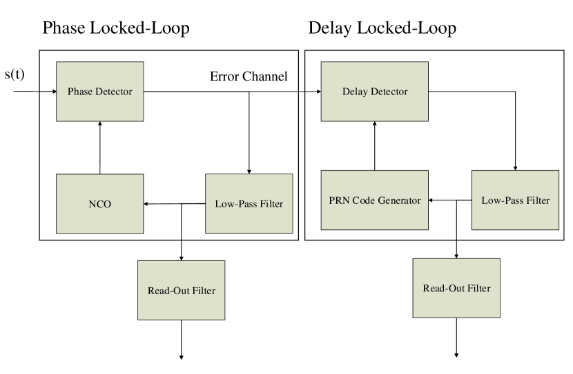
The receiver consists of two main components: the PLL and the DLL being responsible for the carrier tracking, i.e. the phase readout, and code tracking, i.e. the absolute ranging, respectively. The PLL represents a second-order all-digital PLL consisting of a phase detector, a first-order filter and a numerically controlled oscillator (NCO). This generic design is studied extensively in several textbooks [30, 31], and based on linear transfer models, it exhibits a low-pass filter behavior in its closed-loop response, while the error response yields a high-pass filter behavior [31]. Thus, the general principle is as follows. Presuming that the error response bandwidth of the PLL is smaller than the chip rate, the PLL is not able to track chip fluctuations, and the chip sequences will remain in the error channel of the PLL. Consequently, the error channel of the PLL serves as an input to the DLL, cf. Fig. 1. The DLL estimates the time of arrival (TOA) of the incoming PRN sequence based on an early-late discriminator, while a prompt channel is used for data retrieval. The output of the early-late discriminator is thereby low-pass filtered, yielding an update of the TOA for the PRN code generator.
Finally, Table I lists parameters derived from the generic model delineated in Fig. 1. Parameter values have been taken from tables listed in [29] and derived from [12], and where necessary, values not included were added to the table. Thus, these values are regarded as relevant within high-precision space-borne metrology systems, in particular LISA.
| Parameter (Unit) | Symbol | Value |
|---|---|---|
| Modulation index (-) | 0.1 | |
| Chip period (ms) | 0.001 | |
| Sampling rate (MHz) | 80 | |
| Symbol period (ms) | 0.064 | |
| Carrier frequency (Mrad/s) | 30 | |
| PLL bandwidth (closed loop) (kHz) | 250 | |
| DLL bandwidth (closed loop) (Hz) | 10 | |
| Read-out filter PLL (Hz) | 4 | |
| Read-out filter DLL (Hz) | 10 | |
| BPSK early-late spacing () | 0.5 | |
| BOC(1,1) early-late spacing () | 0.2 | |
| Wavelength at heterodyne detection (nm) | 1064 | |
| Responsivity (A/W) | 0.7 |
III Carrier tracking and phase read-out performance
III-A Signal modeling
The measured carrier phase must be of the highest possible accuracy in order to determine relative inter-SC distance changes. As shown in (1), the chip sequence will contribute to the phase measurement noise. Thereby, the data symbol values are not predefined and can be modeled as a random stream. In contrast, the chip values are predefined and follow a fixed pattern. Nevertheless, for sufficiently long PRN sequences, the chip stream will be considered random for the sake of the following development. Consequently, both variables may be modeled as Bernoulli variables , motivating the introduction of a new Bernoulli variable . Thus, the expression for the resulting stochastic noise term is given by:
| (2) |
Noting that the pulse modulation is independent of the index , the former can be expressed according to:
| (3) | ||||
| (4) |
where denotes the convolution operator. In the following section, this term will be used for the calculation of the phase noise measurement performance.
III-B Phase noise
Phase noise is commonly measured as a power spectral density (PSD) , where the variance of phase noise can be deduced from. Modeling the PLL as a linear time-invariant (LTI) system and taking into account the processing according to Fig. 1, the PSD at the readout is given by the noise power spectral density at the input of the PLL filtered by the closed-loop transfer function of the PLL and the read-out filter [31]. Since the sampling rate (80 MHz) of the PLL is significantly larger than its closed-loop bandwidth (250 kHz), the system can be well approximated by a continuous representation in the frequency domain [30]. Both, the closed-loop PLL and the read-out filter exhibit a low-pass filter behavior and may be idealized according to . Hereby, the boxcar function is defined via the Heaviside step function , according to: . Noting that the closed-loop bandwidth of the (250 kHz) exceeds the bandwidth of the read-out filter (Hz – kHz) by orders of magnitude, results in a PSD and the corresponding variance at the readout of:
| (5) | ||||
| (6) |
Thereby, (5) denotes the double-sided PSD, which will be used in the remainder of this paper. In addition, introducing the Fourier pairs , and and exploiting the convolution theorem on (4) yields . Thus the noise power spectral density at the input of the PLL is given by:
| (7) |
Thereby, the brackets , indicate the ensemble average over the Bernoulli variables and . If and are uncorrelated for , the noise power spectral density is solely given by the PSD of the pulse modulation multiplied by the modulation index squared. In this limit, inserting (7) into (5) and (6) yields:
| (8) | ||||
| (9) |
Equations (8) and (9) highlight the impact of the PSD of the pulse modulation on the phase noise performance, which is further quantified in the following section.
III-C Application and numerical verification
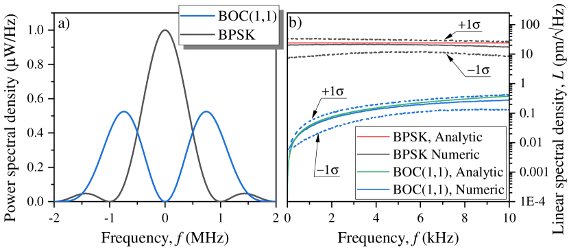
Typical types of pulse modulation schemes are binary phase shift keying (BPSK) and binary offset carrier (BOC). In this discussion, we will restrict ourselves specifically to BPSK-R (where the R indicates a rectangular pulse modulation) and sine-phased BOC(m,n), with . For a BPSK-R modulation with chip period , the PSD is given by: , with . Notably, this function exhibits a maximum at the origin, i.e. at frequencies not being filtered at the phase readout, cf. gray graph in Fig. 2 a). Inserting the PSD of the pulse modulation into 8 and 9 results in:
| (10) | ||||
| (11) | ||||
| (12) | ||||
| (13) |
Thereby, the sine cardinal has been approximated using a Taylor expansion
according to , as .
Importantly, the PSD of the phase noise exhibits a constant value
at low frequencies. Thus, the phase noise can only be reduced via
the chip period and the modulation index. However, when reducing
the modulation index to a level where the residual phase noise becomes
acceptable, the code tracking and associated ranging error, discussed
in the subsequent section, may become in-acceptably large. Similarly,
a smaller chip period may shift large parts of the spectral energy
of the modulation outside the receiver measurement bandwidth. This
situation can however be improved when applying modulation schemes
such as BOC, as shown hereafter.
First introduced by John Betz, BOC(m,n) is characterized by a square
sub-carrier modulation of the chips [32]. The frequency
of the sub-carrier is expressed by the index ,
where represents a reference frequency. The second
index defines the chip rate .
As we restricted the signal to exhibit a constant pulse modulation
, cf. (1), it is necessary to have a sub-carrier
multiple of the chip rate, yielding . With no
loss of generality, we set , expressed as .
Following these presumptions, the PSD of the sine-phased BOC(m,1)
is given by
[32]. In strong contrast to BPSK, the peak of the PSD
is shifted away from the origin, to .
Moreover, the power contribution at the origin reads zero, cf. blue
graph in Fig. 2 a). Finally,
performing similar approximations as for the BPSK modulation results
in a phase noise PSD and variance of:
| (14) | ||||
| (15) | ||||
| (16) | ||||
| (17) |
Strikingly, and in strong contrast to BPSK modulation, the phase noise
PSD for BOC(m,1) reads zero at the origin and increases quadratically.
Consequently, exhibits a maximum at .
The ratio at this maximum between BOC(m,1) and BPSK modulation is
. Thus as long
as , BOC(m,1) modulation exhibits
superior noise performance compared to BPSK modulation. A similar
conclusion holds for the variance.
The effect of the modulation becomes especially noticeable when considering
parameter values base-lined for LISA, see Table I.
In the context of LISA, two modulation schemes have been extensively
discussed in various publications: BPSK and Manchester encoding [33, 10, 11, 12, 27].
Within the ongoing spectral analysis, Manchester encoding can equivalently
be represented as a BOC(1,1). Moreover, in this context, the phase
read-out accuracy is analyzed in terms of displacement noise. For
this purpose, the phase noise is considered as linear spectral density
(LSD), obtained via the square root of the PSD. Converting the phase
noise into displacement noise by multiplication with the conversion
factor , where denotes the wavelength
at the heterodyne detection, yields a single-sided LSD
in , which for BPSK modulation exceeds
the BOC(1,1) LSD by five orders of magnitude.
This significant difference is verified by a numerical PLL simulation,
set up according to the generic model depicted in Fig. 1
and parameter values listed in Table I.
Thereby, 32 randomly generated PRN sequences, modulated either via
BPSK (gray lines) or BOC(1,1) (blue lines) have been considered. Fig.
2 b) illustrates the
single-sided LSD of the displacement noise, where the mean
value (solid lines) and the one-sigma interval (dashed lines) are
depicted after smoothing. Both numerical simulations agree well with
the respective analytical model, exhibiting a constant slope for the
LSD of the BPSK modulation and a linear one for the BOC(1,1) modulation.
Deviations from the analytical model are attributed to the finite
chip sequence length and are found to vanish for infinitely long sequences.
Importantly, these results manifest the superior phase noise performance
of the BOC(1,1) modulation. On the other hand, they exclude BPSK modulation
for the given set of parameter values for applications requiring pico-meter
noise levels at the phase readout.
Until now, the analysis has focused on an ideal heterodyne signal as described in (1). This approach facilitated a performance evaluation based exclusively on architectural design decisions. However, in practical scenarios, the incoming signal often deviates significantly from this ideal model. Consequently, in the following section, we contextualize our analysis with a focus on representative signals, particularly those encountered in the LISA mission.
The heterodyne signal of LISA is given by the beatnote of the received weak signal from a remote spacecraft and a local laser beam, having powers of 350 pW and 1 mW, respectively. These signals interfere at a photodiode, where based on the responsivity (cf. Table I), the incident power is converted into a photocurrent. While redundancy and averaging concepts for photodiode segments have been proposed [34, 35, 36], these aspects are beyond the scope of this paper, and the following analysis considers a single photodiode.
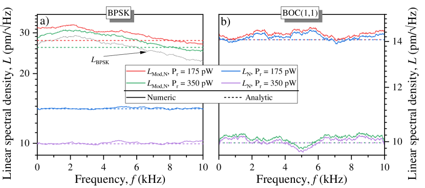
Following the detection principle of LISA, the nominal signal is affected by several noise contributions, see [37]. Tilt-to-length (TTL) coupling noise, arising from the coupling between pupil alignment offsets and spacecraft jitter, is removed in post-processing. Further neglecting stray light coupling noise (very small) and phasemeter internal noise, which depends on the specific hardware and can be made sufficiently small (1 pm/sqrt(Hz)), leaves two dominating contributors, namely shot noise and laser intensity noise. These noise contributions have been incorporated into the incoming signal model applied for the numerical PLL simulations, thus providing a LISA representative signal. Relevant parameter values have been taken from [22]. The resulting displacement noise spectra averaged over 16 randomly generated PRN sequences are depicted in Fig. 3 a) and b) after smoothing. In absence of the PRN modulation, the displacement noise LSD exhibits a flat spectrum, cf. purple curves Fig. 3 a) and b). These spectra are accurately described as uncorrelated summation of analytical formulations for shot noise [12] and laser intensity noise [20, 21, 22]. The same characteristics apply when the power of the incoming laser is halved, as shown by the blue curves in Fig. 3 a) and b). Comparing these results to those obtained for an incoming signal also comprising a PRN-modulated signal component, indicated as , substantiates the relevance of the choice of modulation in the context of LISA.
In Fig. 3 a), we illustrate the
impact of BPSK modulation. The phase noise is strongly dominated by
the modulation, irrespective of the power levels considered, cf. green
and red graphs. The influence becomes clearly evident by comparison
with the gray graph , representing phase noise that
derives solely from the BPSK modulation. In sharp contrast, Fig.
3 b) demonstrates the effect of
BOC(1,1) modulation, which contributes minimally to the overall phase
noise. These findings are consistent with the analytical models,
c.f. dashed lines, while deviations are again attributed to the finite
PRN chip sequence length. Importantly, these results verify the substantial
influence of the modulation scheme on the phase noise performance
for a LISA-representative environment.
Finally, without data transmission, the signal
consists of only periodical spreading sequences, which yield in the
frequency domain a comb around the origin spaced by the inverse of
the code sequence periodicity. Since ,
only the peak at the origin may affect the result, which in the case
of a BOC(m,1) modulation is suppressed, due to the symmetry properties
of the pulse.
IV Code tracking and ranging performance
IV-A Principle of DLL
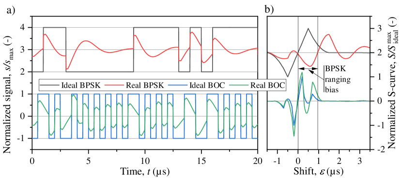
After carrier wiping, a DLL relying on the principle of a non-coherent early-late discriminator, and extensively used in GNSS applications, is capable of tracking the code according to (1). Thereby, the principle of the delay detector, see Fig. 1, relies on two local code replicas – forwarded and delayed in time, where the particular delay of the code replicas, i.e. the early-late spacing, depends strongly on the modulation technique [38, 39]. These replicas are correlated with the incoming signal over one symbol period, followed by a squared magnitude operation, to suppress data polarity. Finally, the difference between early and late correlation yields a value on the so-called S-curve . Thereby, the argument indicates the time shift between the replica and the incoming signal. The gray curve in Fig. 4 b) illustrates a S-curve for an exemplary BPSK-modulated incoming chip sequence which equals its replica. A time segment of the incoming signal, and thus of the replica, is depicted in Fig. 4 a) by the gray curve. For this ideal incoming signal, the zero crossing corresponds to perfect alignment between replica and incoming signal, and is usually considered as the tracking point of the loop, with a tracking range corresponding to the linear regime around the zero crossing. In addition, the blue graph in Fig. 4 b) depicts the S-curve for a BOC(1,1)-modulated signal and its identical replica, whose time segment is portrayed in Fig. 4 b), also by the blue graph. In contrast to the BPSK-modulated S-curve, there are additional stable tracking points, represented by additional zero-crossings within a region of positive slope. These play a key role during loop (re-)acquisition but are not further elaborated in the following discussion. Moreover, the linear range is reduced, due to the necessarily smaller early-late spacing, cf. Table I. Irrespective of the modulation, within the linear range, the time shift between the replica and the incoming signal is obtained via the division of the S-curve value by the constant slope in this regime. In this context, the slope is usually represented as a discriminator gain [38]. Finally, this shift serves as an input to the low-pass filter, which estimates the chip rate used as input to the PRN code generator.
IV-B Signal modeling
In strong contrast to the ideal, i.e. unfiltered, case stated in section IV-A, the architecture depicted in Fig. 1, not only wipes the carrier but also affects the code sequences. Based on standard control theory the code sequences are filtered by the impulse response of the error transfer function of the PLL, yielding the signal , at the input of the DLL. Taking into account the high-pass filter behavior of the error transfer function and the PSD of the two modulation methods, cf. Fig. 2 a), we find that BPSK-modulated sequences are significantly more distorted than BOC(1,1)-modulated sequences. This behavior is illustrated by the red and green curves of Fig 4 a), for BPSK and BOC(1,1) modulation, respectively, which constitute the filtered signals used as input to the DLL. Nonetheless, both signals are characterized by overshoots at the beginning of a chip value transition and strong damping toward the end of the chip. As a consequence, the resulting S-curves, based on the correlation of the filtered signal with an unfiltered replica, differ significantly from the ideal case. In particular, for BPSK modulation, cf. red graph in Fig 4 b), the distortion leads to additional stable tracking points. Besides the shape also the zero crossing of the linear range, i.e. the primary tracking point, is shifted by nearly one chip period, which will be referred to as ranging bias [40]. For BOC(1,1) modulation, alternation in shape and zero crossing are moderate, cf. green graph in Fig 4 b).
Moreover, due to the convolution operation of the filtering, i.e.
due to the filter memory, the symbols not only differ in sign, which
is well accounted for by the magnitude (squared) operation but rather
they depend on the input of the previous symbols. Consequently,
the corresponding S-curve varies over time, yielding a ranging bias
variation.
As a matter of fact, analyzing an uncorrelated chip sequence after
exposure to a high-pass filter, representative for the error transfer
function of the PLL, reveals a correlation time limited to several
chip periods. This behavior is observed for BPSK and BOC(1,1) modulation
for a bandwidth (BW) of 10 - 500 kHz, cf. Fig. 5
d), which appears as relevant PLL bandwidth range considering a chip
rate of 1 MHz. These findings exclude the persistence of correlation
over more than one symbol length (64 chips, cf. Table I).
Therefore, a symbol and its modulated data bit can have at most an
impact on the processing of the succeeding symbol and data bit (memory
effect).
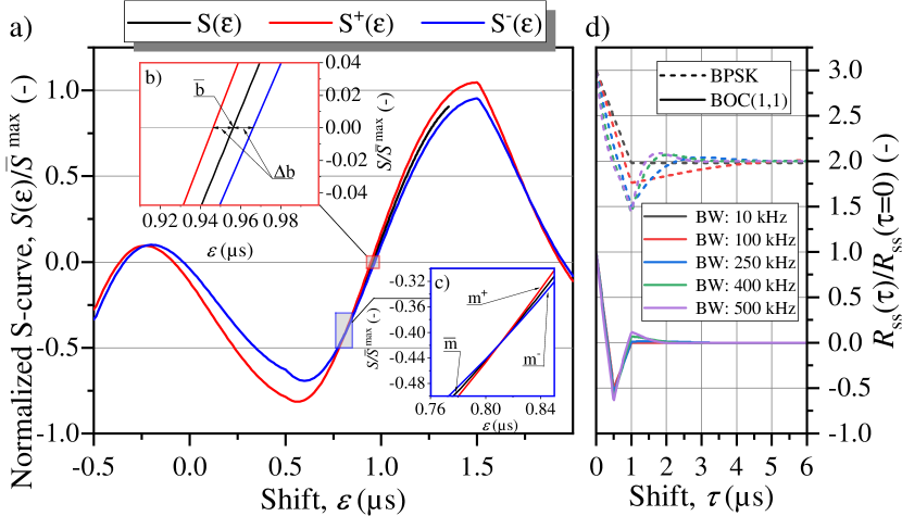
In addition, these findings are affirmed by numerical analysis based on randomly generated PRN sequences and parameter values stated in Table I, revealing that variations of the S-curve are restricted to and , depending on whether the current and previous data symbols exhibit the same () or opposite () value. These S-curves, depicted in Fig. 5 a) for an exemplary BPSK-modulated PRN sequence, promote the introduction of a mean S-curve in the linear range, exhibiting a mean ranging bias as portrayed in Fig. 5 b). Importantly, indicates the mean value based on the x-axis, which can be found via interpolation of in the linear range of and . This leads to a common offset between the mean S-curve and at the zero crossing. Consequently, the ranging bias can be modeled as:
Thereby, the variable expresses the similarity of the current and the previous data symbol, according to:
The boxcar function indicates the variation
in the symbol period . It shall be emphasized, that the mean
ranging bias and the deviation , strongly depend
on the specific code sequence and thus need to be determined numerically.
As long as the mean ranging bias is in the linear range of the S-curve
it only constitutes the tracking point of the DLL, which can be accounted
for by means of calibration and is thus omitted for further discussion.
In contrast, the variation of the ranging bias confines the accuracy
of the tracking loop. In order to identify the corresponding noise
contribution, one can use (2) which
describes the stochastic noise of BPSK modulation for the PLL, and
apply it instead to the DLL analyzed in this section, by establishing
a correspondence between the following parameters: ,
, , leading
to a noise spectral density of
This noise spectral density is low-pass filtered within the DLL, followed by a read-out filter. Approximating both filters as an ideal low-pass filter, the variance at the readout is given by:
| (18) |
Thereby, indicates the read-out filter bandwidth of the DLL, which is assumed to be much smaller than the inverse of the symbol period and smaller or equal to the bandwidth of the DLL low-pass filter. The error of the DLL is usually considered in terms of a ranging error. Thus, the code-tracking error of this semi-analytical model will be defined as , where denotes the speed of light. Similar expressions for the code-tracking error as stated in (18) have been found for alternative DLL implementations [41].
IV-C Application and numerical verification
Analogous to carrier tracking, also for code tracking numerical simulations
have been conducted comparing BPSK and BOC(1,1) modulation schemes
and verifying the semi-analytical model for the code-tracking error
, cf. (18). Besides
the baseline parameters as specified in Table I,
a set of 32 randomly generated PRN sequences has been considered.
In terms of the semi-analytical code-tracking error ,
BOC(1,1) modulation displays a superior performance, differing by
around one order of magnitude compared to the BPSK modulation, cf.
gray data points in Fig. 6
a) and b). This result is expected: as explained in section III,
the BPSK modulation holds its peak spectral energy at the origin,
leading to maximum damping due to the high-pass filter behavior of
the error transfer function of the PLL. On the other hand, the spectral
energy of the BOC(1,1) modulation is shifted away from the carrier,
yielding less spectral confinement, cf. Fig. 2
a), and hence less distorted PRN sequences, see Fig. 4
a) [12]. Consequently, the S-curve of the BOC(1,1)
modulation exhibits a smaller ranging bias variation as
well as an absolute ranging bias that is smaller by approximately
two orders of magnitude.
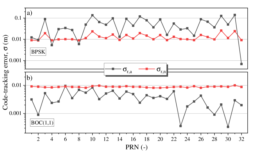
The code-tracking error
of the numerical DLL simulation is based on the variance
of the time shift , once the DLL has been settled.
Interestingly, a significant deviation between modeled and simulated
code-tracking errors is visible irrespective of the modulation scheme.
For BOC(1,1) modulation the numerical code-tracking error is nearly
constant over the set of PRN sequences, exhibiting a value of
9 mm, cf. red data points in Fig. 6
b). Moreover, a correlation to the semi-analytical model is not evident
at first glance. Although the code-tracking error of the model and
the simulation are clearly correlated for BPSK modulation, see red
data points in Fig. 6 a),
deviations are still apparent in terms of the amplitude of the code-tracking
error. These deviations are attributed to two effects: (i) the granularity
of the PRN code generator, and (ii) the varying slopes of the S-curves.
Regarding effect (i), the resolution of the PRN code generator is
confined by the sampling rate of the incoming chip sequence. For BOC(1,1)
modulation, the sampling rate of 80 MHz cannot resolve the ranging
bias variations [42]. Consequently, simulations
exhibit equal code-tracking errors, irrespective of the PRN sequence.
The increased ranging bias variation for the BPSK modulation leads
to a noticeable influence of the bias variation and hence establishes
a correlation between the semi-analytical model and the simulation.
Still, the variations are not fully resolved by the sampling rate.
In addition, effect (ii) is caused by the slope
of the S-curves, necessary for the detection of the time shift
. The DLL deduces the time shift based on the discriminator
gain and thus implies a constant S-curve slope, as delineated in section
IV-A. Because the slopes in the linear
range of the S-curves are not identical, see Fig. 5
c), the TOA estimation induces an error, yielding an additional deviation
from the proposed semi-analytical model.
Further insight into effect (i) is gained through the analytical model
of [42] which investigates the ranging error
resulting from the granularity of the PRN code generator. This model
reveals that for the considered parameter values, the dominant error
results from the granularity of the PRN code generator, i.e. the sampling
error.
In addition, the ranging performance has been evaluated for a LISA
representative signal that is degraded by the external shot noise
and laser intensity noise (see also subsection III-C).
These noise contributions lead to ranging errors that exceed the error
caused by the granularity of the PRN code generator, see above effect
(i). In this case, the ranging error for BOC(1,1) (around several
centimeters, depending on the specific code sequence) is around four
times smaller than for BPSK, which reveals the superiority of BOC(1,1)
encoding for LISA. Comparable findings have been reported in [10, 12].
Nonetheless, both modulation schemes are capable of achieving sub-meter
ranging errors, which is considered sufficient [29].
At this point, it shall be emphasized, that due to the specific TOA detection, pure analytical analysis for the DLL is much more complex compared to the PLL. In particular, this applies to common simplifications, e.g. performed by Betz [41] (or further ones not shown here), which are not applicable in this context. These findings reinforce the necessity of numerical analysis for distinct code sequences and receiver architectures.
V Conclusion
This paper revealed the compelling influence of the modulation scheme on the performance of sequential carrier- and code-tracking receiver architectures foreseen for future space-borne metrology systems.
A generic sequential PLL–DLL design including a representative signal consisting of a carrier modulated by code sequences has been introduced, enabling a novel analysis of the performance losses resulting exclusively from the architecture itself. Thereby, carrier- and code-tracking analyses have been conducted separately. In the former case a generic model has been introduced, exploiting the distinct parameter range and estimating the phase noise for an arbitrary but periodic modulation scheme. Thereby, the PSD of the pulse modulation within the read-out bandwidth has been identified as the main driver for phase noise. This model, subjected to BPSK and BOC(1,1) modulation revealed the superior phase noise performance of the latter. Moreover, it excluded BPSK as a modulation scheme for space-borne metrology systems demanding pico-meter noise levels at the phase readout, considering the stated set of parameter values. Finally, these results have been verified by numerical PLL simulations, which agreed well with the analytical model regardless of the modulation scheme.
Analysis of the code tracking has been focused on the TOA estimation,
taking into account the concept of the S-curve. Thereby, a varying
S-curve due to the PLL filtering of the incoming signal has been observed,
differing in shape and zero crossing from the ideal case. Remarkably,
analyses revealed that variations of the S-curve can be reduced to
two cases, depending on whether the current and previous data symbols
exhibit the same or opposite value, enabling a similar mathematical
approach for the code tracking as used before for the phase noise.
Finally, the model was compared with numerical DLL simulations. Differences
became apparent, which were primarily attributed to the granularity
of the PRN code generator. While both modulation schemes exhibited
sub-meter ranging errors, BOC(1,1) modulation surpasses but at least
equals the performance of the BPSK modulation.
Sequential carrier and code tracking architectures are thus in principle
capable of serving as receivers for high-precision space-borne measurement
systems, but performance is significantly affected by the modulation
scheme. While the analysis was restricted to one data symbol per PRN
sequence, it can easily be extended to analyses of PRN sequences exhibiting
multiple data symbols, facilitating higher data rates.
Acknowledgment
The authors thank T. Ziegler and S. Delchambre for their support and fruitful discussions.
References
- [1] K. Danzmann and the LISA Study Team, “LISA - an ESA cornerstone mission for the detection and observation of gravitational waves,” Adv. Space Res., vol. 32, no. 7, pp. 1233–1242, 2003.
- [2] Z. Luo, Y. Wang, Y. Wu, W. Hu, and G. Jin, “The Taiji program: A concise overview,” Prog. Theor. Exp. Phys., vol. 2021, no. 5, 2020, Art. no. 05A108.
- [3] J. Mei, Y.-Z. Bai, J. Bao, E. Barausse, L. Cai, E. Canuto, B. Cao, W.-M. Chen, Y. Chen, Y.-W. Ding et al., “The tianqin project: current progress on science and technology,” Prog. Theor. Exp. Phys., vol. 2021, no. 5, 2021, Art. no. 05A107.
- [4] S. Kawamura, M. Ando, N. Seto, S. Sato, M. Musha, I. Kawano, J. Yokoyama, T. Tanaka, K. Ioka, T. Akutsu et al., “Current status of space gravitational wave antenna decigo and b-decigo,” Prog. Theor. Exp. Phys., vol. 2021, no. 5, 2021, Art. no. 05A107.
- [5] K. Danzmann, T. A. Prince et al., “LISA assessment study report (yellow book),” European Space Agency, Tech. Rep. ESA/SRE(2011)3, 2011.
- [6] M. Tinto and S. V. Dhurandhar, “Time-delay interferometry,” Living Rev Relativ, vol. 24, no. 1, pp. 1–73, 2021.
- [7] M. Muratore, D. Vetrugno, and S. Vitale, “Revisitation of time delay interferometry combinations that suppress laser noise in LISA,” Classical Quantum Gravity, vol. 37, no. 18, 2020, Art. no. 185019.
- [8] N. Houba, S. Delchambre, T. Ziegler, G. Hechenblaikner, and W. Fichter, “LISA spacecraft maneuver design to estimate tilt-to-length noise during gravitational wave events,” Phys. Rev. D, vol. 106, no. 2, 2022, Art. no. 022004.
- [9] G. Heinzel, J. J. Esteban, S. Barke, M. Otto, Y. Wang, A. F. Garcia, and K. Danzmann, “Auxiliary functions of the LISA laser link: ranging, clock noise transfer and data communication,” Classical Quantum Gravity, vol. 28, no. 9, 2011, Art. no. 094008.
- [10] A. Sutton, K. McKenzie, B. Ware, and D. A. Shaddock, “Laser ranging and communications for LISA,” Opt. Express, vol. 18, no. 20, pp. 20 759–20 773, 2010.
- [11] J. J. Esteban, A. F. García, S. Barke, A. M. Peinado, F. G. Cervantes, I. Bykov, G. Heinzel, and K. Danzmann, “Experimental demonstration of weak-light laser ranging and data communication for LISA,” Opt. Express, vol. 19, no. 17, pp. 15 937–15 946, 2011.
- [12] J. J. Esteban Delgado, “Laser Ranging and Data Communication for the Laser Interferometer Space Antenna,” Ph.D. dissertation, Universidad de Granada, 2012.
- [13] D. Shaddock, B. Ware, P. G. Halverson, R. E. Spero, and B. Klipstein, “Overview of the LISA Phasemeter,” AIP Conf. Proc., vol. 873, no. 1, pp. 654–660, Nov. 2006.
- [14] Y.-R. Liang, Y.-J. Feng, G.-Y. Xiao, Y.-Z. Jiang, L. Li, and X.-L. Jin, “Experimental scheme and noise analysis of weak-light phase locked loop for large-scale intersatellite laser interferometer,” Rev. Sci. Instrum., vol. 92, no. 12, p. 124501, Dec. 2021.
- [15] Y. Li, C. Wang, L. Wang, H. Liu, and G. Jin, “A laser interferometer prototype with Pico-Meter measurement precision for taiji space gravitational wave detection missionin china,” Microgravity Sci. Technol., vol. 32, no. 3, pp. 331–338, Jun. 2020.
- [16] H.-S. Liu, Y.-H. Dong, Y.-Q. Li, Z.-R. Luo, and G. Jin, “The evaluation of phasemeter prototype performance for the space gravitational waves detection,” Rev. Sci. Instrum., vol. 85, no. 2, 2014, Art. no. 024503.
- [17] O. Gerberding, C. Diekmann, J. Kullmann, M. Tröbs, I. Bykov, S. Barke, N. C. Brause, J. J. Esteban Delgado, T. S. Schwarze, J. Reiche, K. Danzmann, T. Rasmussen, T. V. Hansen, A. Enggaard, S. M. Pedersen, O. Jennrich, M. Suess, Z. Sodnik, and G. Heinzel, “Readout for intersatellite laser interferometry: Measuring low frequency phase fluctuations of high-frequency signals with microradian precision,” Rev. Sci. Instrum., vol. 86, no. 7, 2015, Art. no. 074501.
- [18] B. J. Meers and K. A. Strain, “Modulation, signal, and quantum noise in interferometers,” Phys. Rev. A, vol. 44, pp. 4693–4703, Oct. 1991.
- [19] T. M. Niebauer, R. Schilling, K. Danzmann, A. Rüdiger, and W. Winkler, “Nonstationary shot noise and its effect on the sensitivity of interferometers,” Phys. Rev. A, vol. 43, pp. 5022–5029, May 1991.
- [20] G. Hechenblaikner, “Common mode noise rejection properties of amplitude and phase noise in a heterodyne interferometer,” J. Opt. Soc. Am. A, vol. 30, no. 5, pp. 941–947, May 2013.
- [21] L. Wissel, A. Wittchen, T. S. Schwarze, M. Hewitson, G. Heinzel, and H. Halloin, “Relative-intensity-noise coupling in heterodyne interferometers,” Phys. Rev. Appl., vol. 17, p. 024025, Feb. 2022.
- [22] L. Wissel, O. Hartwig, J. Bayle, M. Staab, E. Fitzsimons, M. Hewitson, and G. Heinzel, “Influence of laser relative-intensity noise on the laser interferometer space antenna,” Phys. Rev. Appl., vol. 20, p. 014016, Jul. 2023.
- [23] Y.-R. Liang, H.-Z. Duan, X.-L. Xiao, B.-B. Wei, and H.-C. Yeh, “Note: Inter-satellite laser range-rate measurement by using digital phase locked loop,” Rev. Sci. Instrum., vol. 86, no. 1, 2015, Art. no. 016106.
- [24] F. Ales, O. Mandel, P. Gath, U. Johann, and C. Braxmaier, “A phasemeter concept for space applications that integrates an autonomous signal acquisition stage based on the discrete wavelet transform,” Rev. Sci. Instrum., vol. 86, no. 8, 2015, Art. no. 084502.
- [25] Y.-R. Liang, “Note: A new method for directly reducing the sampling jitter noise of the digital phasemeter,” Rev. Sci. Instrum., vol. 89, no. 3, 2018, Art. no. 036106.
- [26] J. J. Esteban, I. Bykov, A. F. G. Marín, G. Heinzel, and K. Danzmann, “Optical ranging and data transfer development for LISA,” J. Phys.: Conf. Ser., vol. 154, no. 1, 2009, Art. no. 012025.
- [27] A. J. Sutton, K. McKenzie, B. Ware, G. de Vine, R. E. Spero, W. Klipstein, and D. A. Shaddock, “Improved optical ranging for space based gravitational wave detection,” Classical Quantum Gravity, vol. 30, no. 7, p. 075008, Mar. 2013.
- [28] S. Xie, H. Zeng, Y. Pan, D. He, S. Jiang, Y. Li, Y. Du, H. Yan, and H. chi Yeh, “Bi-directional prn laser ranging and clock synchronization for tianqin mission,” Opt. Commun., vol. 541, p. 129558, 2023.
- [29] S. Barke, N. Brause, I. Bykov, J. J. Esteban Delgado, A. Enggaard, O. Gerberding et al., “LISA Metrology System - Final Report,” no. ESA ITT AO/1-6238/10/NL/HB, 2014.
- [30] D. R. Stephens, Phase-Locked Loops for Wireless Communications: Digital and Analog Implementation. Springer New York, NY, 2002.
- [31] F. M. Gardner, Phaselock Techniques, 3rd ed. John Wiley & Sons, Inc., Hoboken, New Jersey, 2005.
- [32] J. W. Betz, “Binary offset carrier modulations for radionavigation,” Navigation, vol. 48, no. 4, pp. 227–246, 2001.
- [33] V. Wand, “Interferometry at low frequencies: optical phase measurement for LISA and LISA Pathfinder,” Ph.D. dissertation, Gottfried Wilhelm Leibniz Universität Hannover, 2007.
- [34] E. Morrison, B. J. Meers, D. I. Robertson, and H. Ward, “Automatic alignment of optical interferometers,” Appl. Opt., vol. 33, no. 22, pp. 5041–5049, Aug. 1994.
- [35] E. Morrison, B. J. Meers, D. I. Robertson, and H. Ward, “Experimental demonstration of an automatic alignment system for optical interferometers,” Appl. Opt., vol. 33, no. 22, pp. 5037–5040, Aug. 1994.
- [36] G. Heinzel, M. D. Álvarez, A. Pizzella, N. Brause, and J. J. E. Delgado, “Tracking length and differential-wavefront-sensing signals from quadrant photodiodes in heterodyne interferometers with digital phase-locked-loop readout,” Phys. Rev. Appl., vol. 14, p. 054013, Nov. 2020.
- [37] LISA Consortium, “LISA Performance Model and Error Budget,” 2021, LISA-LCST-INST-TN-003. Technical Report 2.1, ESA.
- [38] J. W. Betz, “Design and Performance of Code Tracking for the GPS M Code Signal,” in Proceedings of the 13th International Technical Meeting of the Satellite Division of The Institute of Navigation (ION GPS 2000), Salt Lake City, UT,, 2000, pp. 2140–2150.
- [39] A. J. Van Dierendonck, P. Fenton, and T. Ford, “Theory and Performance of Narrow Correlator Spacing in a GPS Receiver,” Navigation, vol. 39, no. 3, pp. 265–283, 1992.
- [40] J. W. Betz, “Effect of Linear Time-Invariant Distortions on RNSS Code Tracking Accuracy,” in Proceedings of the 15th International Technical Meeting of the Satellite Division of The Institute of Navigation (ION GPS 2002), Portland, OR,, 2002, pp. 1636–1647.
- [41] J. W. Betz and K. R. Kolodziejski, “Generalized theory of code tracking with an early-late discriminator part i: Lower bound and coherent processing,” IEEE Trans. Aerosp. Electron. Syst., vol. 45, no. 4, pp. 1538–1556, 2009.
- [42] P. Euringer, G. Hechenblaikner, F. Soualle, S. Delchambre, T. Ziegler, and W. Fichter, “Modeling of digital receiver-induced ranging bias variations in the context of high precision space-borne metrology systems,” in Proc. SPIE 12619, Modeling Aspects in Optical Metrology IX, 2023, p. 126190A.