Residual QPAS subspace (ResQPASS) algorithm for bounded-variable least squares (BVLS) with superlinear Krylov convergence

Abstract

This paper presents the Residual QPAS Subspace (ResQPASS) method that solves large-scale linear least-squares problems with bound constraints on the variables. The problem is solved by creating a series of small projected problems with increasing size. We project on the basis spanned by the residuals. Each projected problem is solved by the QPAS method that is warm-started with the working set and the solution of the previous problem. The method coincides with conjugate gradients (CG) applied to the normal equations when none of the constraints is active. When only a few constraints are active the method converges, after a few initial iterations, as the CG method. Our analysis links the convergence to Krylov subspaces. We also present an efficient implementation where the matrix factorizations using QR are updated over the inner iterations and Cholesky over the outer iterations.

49N45, 65K05, 65F10, 90C20

1 Introduction

Inverse problems reconstruct an unknown object from measurements based on a mathematical model that describes the data acquisition. It inverts the measured signal into information about an unknown object. A well known inverse problem is computed tomography (CT), where an unknown object is reconstructed from a projection sinogram. In algebraic reconstruction the problem is formulated as a linear least squares problem, $\min_{x\in\mathbb{R}^{n}}\|Ax-b\|^{2}_{2}$, that minimizes the mismatch between the data and model. Here, the matrix $A\in\mathbb{R}^{m\times n}$ models the propagation of the X-rays through the object [8], $x\in\mathbb{R}^{n}$ describes the unknown pixel values and $b\in\mathbb{R}^{m}$ is the vector with noisy measurements.

However, since $A$ is ill-conditioned, e.g. a vector with oscillating $+1$,$-1$ pixel values is in the near null space, the straightforward least-squares solution, $x=(A^{T}A)^{-1}A^{T}b$ will be contaminated due to the noise in the measurements [6]. To avoid overfitting to the noise, regularization techniques are used. For example, in Tikhonov regularization [2] the reconstruction problem is replaced by $\min_{x\in\mathbb{R}^{n}}\|Ax-b\|_{2}^{2}+\lambda\|Lx\|_{2}$ where a regularization term with a regularization operator $L$ is added. The regularization parameter $\lambda>0$ can be tuned such that the Morozov discrepancy principle is satisfied [12]. In LASSO [17] the problem becomes $\min_{x\in\mathbb{R}^{n}}\|Ax-b\|_{2}^{2}+\lambda\|Lx\|_{1}$. The regularization term now uses a $\ell_{1}$-norm that promotes sparsity in the solution. Elastic net [20] combines the $\ell_{1}$-norm and the $\ell_{2}$-norm in the regularization.

The focus of this paper is on an alternative regularization technique where bounds on the variables limit the sensitivity of the solution to measurement noise. We solve

(1) $$\min_{l\leq x\leq u}\,\frac{1}{2}\|Ax-b\|_{2}^{2},$$

where the lower and bounds are vectors $l,u\in\mathbb{R}^{n}$. This problem is known as the bounded-variable least squares (BVLS) that can, for example, be solved by the Stark-Parker algorithm [16]. When only lower bounds are used, it is a non-negative least squares (NNLS) problem [9]. Note that also the Lasso problem can be formulated as a non-negative QP problem.

This results in a constrained quadratic programming (QP) problem. We will call the objective $f(x)\coloneqq\frac{1}{2}\|Ax-b\|_{2}^{2}$. In tomography, for example, the bounds limit the pixel values of the reconstructed object.

The Karush-Kuhn-Tucker (KKT) optimality conditions [14] for Eq. 1 are

(2a) $$A^{T}(Ax-b)-\lambda+\mu =0$$

(2b) $$\lambda_{i}(x_{i}-\ell_{i}) =0 i\in\{1,\ldots,n\}$$

(2c) $$\mu_{i}(u_{i}-x_{i}) =0 i\in\{1,\ldots,n\}$$

(2d) $$\ell_{i}\leq x_{i} \leq u_{i} i\in\{1,\ldots,n\}$$

(2e) $$(\lambda,\mu) \geq 0$$

where $\lambda\in\mathbb{R}^{n}$ and $\mu\in\mathbb{R}^{n}$ are vectors with Lagrange multipliers associated, respectively, for the lower and upper bounds.

The state-of-the-art method to solve a general large-scale QP or linear programming (LP) problem are interior-point methods [14, 3], where each iteration a weighted sparse-matrix needs to be factorized by a Cholesky factorization. For large-scale LP problems column generation [11] is a technique where the block structure of the matrix is exploited by writing the solution as a convex combination of solutions of subproblems. This results in an iterative method that alternates between solving a master problem, which finds the coefficients of the convex combination, and a new subproblem that expands the vectors for the convex combination.

In this paper we use a linear combination of residuals as an approximation to the solution. Each iteration we solve a projected problem, similar to the master problem in column generation. The use of residuals as a basis for the expansion is common in Krylov methods.

The use of Krylov methods is widespread in scientific computing. They are attractive for applications with sparse matrices. Since a sparse-matrix vector product, $Av$, is computationally inexpensive and paralellisable, it is cheap to generate a Krylov subspace. The convergence of Krylov methods is well understood and various preconditioning techniques such as multigrid or incomplete factorisation techniques can accelerate the convergence. For a review of Krylov methods and various preconditioning techniques we refer to [10, 15].

For inverse problems that typically involve a non-square matrix Golub-Kahan bi-diagonalization is used [1]. It searches a solution in the subspace formed by the matrix powers,

(3) $$\mathcal{K}_{k}(A^{T}A,A^{T}b)=\text{span}\left\{A^{T}b,(A^{T}A)A^{T}b,\ldots,(A^{T}A)^{k-1}A^{T}b\right\}.$$

So far as we know Krylov methods have not been extended to include lower and upper bounds on the variables. There is a literature on enforcing non-negative constraints in [13].

In this paper we make the following contributions. We propose a new subspace method that uses the residuals from the KKT condition, (2). Each iteration we solve a small projected QP problem with dense matrices using the active-set QP algorithm (QPAS). When only a few bounds are active in the solution we observe superlinear convergence behavior. We explain this superlinear behavior by making the link to Krylov convergence theory. From a certain point on, the residuals can be written as polynomials of the normal matrix applied to a vector and the convergence is determined by the Ritz values of the projected matrix.

In addition, we contribute an efficient implementation that uses warm starting, as the basis is expanded, and updates the factorization of the matrices that need to be solved each iteration. Additional recurrence relations gives further improvements.

The analysis of the propagation of the rounding errors and the final attainable accuracy is not part of this study and will be the subject of a future paper.

The outline of the paper is as follows. In Section 2 we derive the algorithm and prove some properties of the basis. Section 3 discusses several ways to speed up the algorithm and Section 4 discusses some synthetic numerical experiments representative for different application areas. We conclude in Section 5.

2 The Residual QPAS Subspace method and its convergence

In this section we introduce the methodology and analyse the convergence.

2.1 Residual QPAS Subspace Method

We propose to solve Eq. 1 by iteratively solving a projected version of the problem. We write the solution $x_{k}=V_{k}y_{k}$ with a zero initial guess.

Definition 2.1.

The residual QPAS subspace iteration for a $A\in\mathbb{R}^{m\times n}$, $b\in\mathbb{R}^{m}$ and $l,u\in\mathbb{R}^{n}$, lower and upper bounds such that $l\leq 0\leq u$, generates a series of guesses $\{x_{k}\}_{k\in\mathbb{N}}$ that are solution of

(4) $$x_{k}=\operatorname*{argmin}_{x\in\operatorname{span}\{r_{0},\ldots,r_{k-1}\}} \|Ax-b\|_{2}^{2}$$

s.t. $$\,l\leq x\leq u$$

where

(5) $$r_{k}:=A^{T}(Ax_{k}-b)-\lambda_{k}+\mu_{k}$$

and $\lambda_{k},\mu_{k}\in\mathbb{R}^{n}$ are the Lagrange multipliers associated with the lower and upper bound. The feasible initial guess is $x_{0}=0$ and $r_{0}:=-A^{T}b$.

Remark 2.2.

The condition $l\leq 0\leq u$, to ensure feasibility of $x_{0}$, does not imply any restrictions on the problems that can be solved. The problem with arbitrary $l<u$, can always be shifted, such that $l\leq 0\leq u$ holds.

A high level implementation of this algorithm is given in algorithm 1 and a more detailed implementation in algorithm 3.

If $V_{k}\in\mathbb{R}^{n\times k}$ with $r_{k}$ is defined in (5), is a basis for $\text{span}\{r_{0},\ldots,r_{k-1}\}$, the optimization problem at iteration $k$ is

(6) $$\min_{y_{k}\in\mathbb{R}^{k}} \quad\frac{1}{2}\|AV_{k}y_{k}-b\|_{2}^{2}$$

s.t. $$\quad\ell_{i}\leq[V_{k}y_{k}]_{i}\leq u_{i}\quad i\in\{1,\ldots,m\}.$$

The coefficients $y_{k}\in\mathbb{R}^{k}$ are the projections of the unknown solution on $V_{k}$ and $k$ is the dimension of the subspace.

The corresponding KKT conditions for (6) are now:

(7a) $$V_{k}^{T}A^{T}(AV_{k}y_{k}-b)-V_{k}^{T}\lambda_{k}+V_{k}^{T}\mu_{k} =0$$

(7b) $$(\lambda_{k})_{i}([V_{k}y_{k}]_{i}-\ell_{i}) =0 i\in\{1,\ldots,n\}$$

(7c) $$(\mu_{k})_{i}(u_{i}-[V_{k}y_{k}]_{i}) =0 i\in\{1,\ldots,n\}$$

(7d) $$\ell_{i}\leq[V_{k}y_{k}]_{i} \leq u_{i} i\in\{1,\ldots,n\}$$

(7e) $$(\lambda_{k},\mu_{k}) \geq 0.$$

We call the active set the set $\mathcal{A}_{k}\subset\{1,\ldots,n\}$ where the bound constraint, (7d), become equalities.

As is done in Krylov-type methods (see [10]) we will use residuals $r_{k}$ to expand our basis. For every iteration $k$, the basis of the subspace becomes $V_{k}=\begin{bmatrix}r_{0}/\|r_{0}\|&\cdots&r_{k-1}/\|r_{k-1}\|\end{bmatrix}$. This choice of residual basis is natural for Krylov methods such as conjugate gradients (CG). We will prove their pairwise orthogonality in lemma 2.3, how this is a generalization of Krylov in lemma 2.7 and how there is asymptotic Krylov convergence in lemma 2.19.

Lemma 2.3 (Orthogonality of $r_{k}$ for optimal solution of projected system).

If $y^{*}_{k}\in\mathbb{R}^{k}$ is an optimal solution of Eq. 6 then the $\{r_{k}\}_{k\in\{1,2\ldots\}}$ as defined in Eq. 5 are pairwise orthogonal.

Proof 2.4.

If $y^{*}_{k}$ is optimal, the KKT conditions (7) hold. The stationarity conditions Eq. 7a can be rewritten as follows:

(8) $$V_{k}^{T}\left(A^{T}(AV_{k}y_{k}-b)-\lambda_{k}+\mu_{k}\right)=V_{k}^{T}r_{k}=0.$$

Since $V_{k}$ is a basis for $\text{span}[r_{0},r_{1},\ldots r_{k-1}]$, this proofs the orthogonality of the $r_{k}$’s to $V_{k}$.

Lemma 2.5 (Orthogonality of $r_{k}$ for feasible solution of projected system).

If $y_{k},\lambda_{k},\mu_{k}$ is a feasible solution of 7a then the $\{r_{k}\}_{k\in\{1,2\ldots\}}$ as defined in Eq. 5 are pairwise orthogonal.

Proof 2.6.

Again, Eq. 7a can be rewritten as as a orthogonality condition. So a feasible solution of the stationarity condition is orthogonal to the previous residuals.

There exists a natural link between the residuals in Eq. 5 and the Krylov-subspace.

Lemma 2.7 (Generalization of Krylov-subspace).

In the unconstrained case none of the bounds of Eq. 6 are ever active, we get:

(9) $$\mathcal{V}_{k+1}\coloneqq\operatorname{span}\left\{r_{0},r_{1},\ldots,r_{k}\right\}\cong\mathcal{K}_{k+1}(A^{T}A,r_{0})\coloneqq\operatorname{span}\left\{r_{0},A^{T}Ar_{0},\ldots,\left(A^{T}A\right)^{k}r_{0}\right\}.$$

With $r_{k}$ defined as in Eq. 5.

Proof 2.8.

If the problem is unconstrained, there are no Lagrange multipliers $\lambda$ and $\mu$. If none of the constraints are ever active, the complementarity condition Eqs. 7b and 7c ensures that $\lambda=0=\mu$. Thus our residuals $r_{k}$ simplify to

(10) $$r_{k}=A^{T}(AV_{k}y_{k}-b).$$

For $k=1$, the statement is trivial. Assume Eq. 9 holds for $k=j-1$. Then

(11) $$r_{k} =A^{T}A\begin{bmatrix}r_{0}&r_{1}&\cdots&r_{k-1}\end{bmatrix}\begin{bmatrix}y_{0}\\ \vdots\\ y_{k-1}\end{bmatrix}-A^{T}b$$

(12) $$=A^{T}A\left(y_{0}r_{0}+\cdots+y_{k-1}r_{k-1}\right)+r_{0}$$

(13) $$=r_{0}+y_{0}A^{T}Ar_{0}+\cdots+y_{k-1}A^{T}Ar_{k-1}.$$

Example 2.9.

If we now compare our method applied to the unconstrained problem, with the implementation of CG in matlab (pcg) applied to $A^{T}Ax=A^{T}b$, we notice in figure 1 that they converge similarly. This also suggests the possibility of preconditioning.

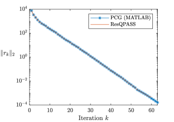
Figure 1: Comparison of conjugate gradients and ResQPASS for an unconstrained least squares problem. Here CG is applied to the normal equation $A^{T}A=A^{T}b$.

Example 2.10.

Let us look at an example with a limited number of active constraints, where we have control over the maximal number of active constraints. Consider the least-squares problem $\min\|Ax-b\|_{2}^{2}$ with $A\in\mathbb{R}^{1000\times 600}$ where 4% of the entries are 1 and the rest are 0. Let half of the entries of the exact solution $x^{*}$ be 0 and the others be $\pm 1$. Finally, let $b=Ax$. Let $m_{\max}$ be the maximal number of active constraints, then we add the following constraints to the problem:

(14) $$-\frac{1}{2}\|x^{*}_{i}\|-0.01\leq x_{i}\leq\frac{1}{2}\|x_{i}^{*}\|+0.01\qquad i\in\{1,\ldots,m_{\max}\}$$

The $0.01$ offset is to ensure that the lower- and upper bounds are never equal. The experiment is performed for $m_{\max}=\{0,1,2,4,8,16,32,64,128\}$. From the results in figure 2 we can conjecture that the method has two steps: discovery of the active set and Krylov convergence. Notice that the discovery phase takes a number of iterations, roughly equal to $m_{\max}$, or the number of active constraints. The number of iterations for the Krylov convergence is always more or less the same as for the unconstrained problem (where there is no discovery phase).

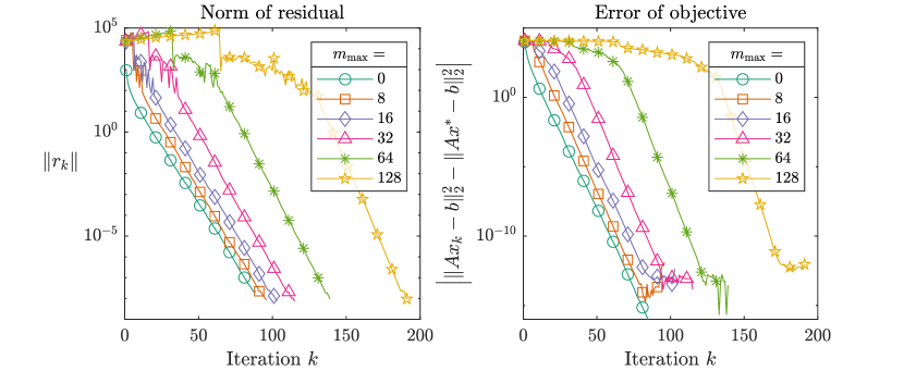
Figure 2: This figure illustrates the convergence behavior for different number of active constraints. The residual and objective behave similar to the unbounded ($m_{\max}=0$, Krylov convergence) case, with a delay that is roughly equal to $m_{\max}$, the number of active constraints in the problem.

2.2 Convergence theory

Algorithm 1 Residual QPAS subspace (ResQPASS)

1:$A\in\mathbb{R}^{m\times n},b\in\mathbb{R}^{m}$, $l,u\in\mathbb{R}^{n}$

2:$r_{0}=A^{T}b$

3:$V_{1}=[r_{0}/\|r_{0}\|]$

4:$y_{1}=0$

5:$\mathcal{W}_{1}=\emptyset$

6:for $k=1,2,\ldots,m$ do

7:     $y_{k}^{*},\lambda_{k},\mu_{k},\mathcal{W}_{k}^{*}\leftarrow$ Solve Eq. 6 using qpas, with initial guess $y_{k}$ and initial working set $\mathcal{W}_{k}$

8:     $r_{k}=A^{T}\left(AV_{k}y_{k}^{*}-b\right)-\lambda_{k}+\mu_{k}$

9:     if  $\|r_{k}\|_{2}\leq tol$ then

10:         $x=V_{k}y_{k}$ break;

11:     end if

12:     $V_{k+1}\leftarrow\begin{bmatrix}V_{k}&r_{k}/\|r_{k}\|\end{bmatrix}$

13:     $y_{k+1}\leftarrow\begin{bmatrix}(y_{k}^{*})^{T}&0\end{bmatrix}^{T}$

14:     $\mathcal{W}_{k+1}\leftarrow\mathcal{W}_{k}^{*}$

15:end for

Based in these observations we develop a convergence theory.

Lemma 2.11.

Let $\lambda_{k},\mu_{k}\in\mathbb{R}^{n}$ be the solution for the Lagrange multipliers of the projected KKT conditions, (7) for iteration $k$. Let $V_{k}\in\mathbb{R}^{n\times k}$ be the subspace generated by the residuals $r_{k}$, as in Definition 2.1. Then there exists an iteration $0<k_{0}\leq n$ such that for all iterations $k$, where $k_{0}\leq k$ holds, that $-\lambda_{k}+\mu_{k}\in\operatorname{span}([V_{k_{0}},A^{T}AV_{k_{0}-1}])$.

Proof 2.12.

$V_{k}$ can maximally grow to $n$ independent vectors and then ${\text{span}\{V_{n}\}=\mathbb{R}^{n}}$. In that case, the $-\lambda+\mu\in\mathbb{R}^{n}$, solutions of (2), are in $\text{span}(V_{n})$.

The number of active constraints is determined by the number of non-zeros in $-\lambda+\mu$, solutions of (2) and it is usually much smaller then $n$.

Because we solve (7) with a basis, the number of active bounds in $l\leq V_{k}y_{k}\leq u$ we have at least $k$ equalities. So the number of non-zeros in $-\lambda_{k}+\mu_{k}$, at iteration $k$, is at least $k$.

We can construct the following subspace of $\mathbb{R}^{n}$

(15) $$\text{span}\left\{-\lambda_{1}+\mu_{1},-\lambda_{2}+\mu_{2},\ldots,-\lambda_{k}+\mu_{k}\right\},$$

where the first vector has, at least, one non-zero, the second at least two, and so on. At some point, this space spans the exact active set of the problem and also $-\lambda^{*}+\mu^{*}$, the solution of the full problem (2), can be written as a linear combination of the vectors in this subspace. Once these vectors span the space of the active set, this basis does not expand anymore and linear dependence appears.

By construction, see definition of the residual vector (5), these vectors in (15) are equivalent with the following vectors

(16) $$\text{span}\left\{r_{1}-A^{T}(AV_{1}y_{1}-b),r_{2}-A^{T}(AV_{2}y_{2}-b),\ldots,r_{k}-A^{T}(AV_{k}y_{k}-b)\right\}.$$

As soon as linear dependence appears in (15), the last vector, $-\lambda_{k}+\mu_{k}$, can be written as a linear combination of the previous vectors. This means that there are coefficients $a_{l}\in\mathbb{R}$ such that

(17) $$-\lambda_{k}+\mu_{k}=r_{k}-A^{T}AV_{k}y_{k}=\sum_{l=1}^{k-1}(r_{l}-A^{T}(AV_{l}y_{l}-b))a_{l}\in\text{span}[V_{k},A^{T}AV_{k-1}],$$

where we use that $-A^{T}b=V_{k_{0}}\|A^{T}b\|e_{1}$, since we start with $x_{0}=0$.

At the first iteration $k$, where this linear dependence appears, we set $k_{0}:=k-1$.

The lemma 2.11 means that, for an iteration $k_{0}\leq k$, there is a $\alpha^{(k)}\in\mathbb{R}^{k_{0}}$ and a $\beta^{(k)}\in\mathbb{R}^{k_{0}-1}$ such that we can write the residual as

(18) $$r_{k} =A^{T}(AV_{k}y_{k}-b)-\lambda_{k}+\mu_{k}$$

$$=A^{T}AV_{k}y_{k}+V_{k_{0}}\alpha^{(k)}+A^{T}AV_{k_{0}-1}\beta^{(k)}$$

$$=A^{T}AV_{k}(y_{k}+(\beta^{(k)},0)^{T})+V_{k_{0}}\alpha^{(k)}\quad\forall k\geq k_{0}.$$

Here we use again that $A^{T}b=V_{k_{0}}\|A^{T}b\|e_{1}$, since we start with $x_{0}=0$. Since $\lambda_{k}$ and $\mu_{k}$ can still change with the iteration, the coefficients $\alpha^{(k)}$ and $\beta^{(k)}$ depend on $k$.

Lemma 2.13.

If $y_{k}\in\mathbb{R}^{k}$ and $\lambda_{k},\mu_{k}\in\mathbb{R}^{n}$ are the solution of (7) and the iteration $k\geq k_{0}$ is such that 2.11 holds, then there are $\gamma_{i}^{(k)}\in\mathbb{R}^{k_{0}}$ with $i\in\{0,\ldots,k-k_{0}\}$ such that the residual is

(19) $$r_{k}=A^{T}(AV_{k}y_{k}-b)-\lambda_{k}+\mu_{k}=\sum_{m=0}^{k-k_{0}+1}(A^{T}A)^{m}V_{k_{0}}\gamma^{(k)}_{m}\quad\forall k\geq k_{0}.$$

Proof 2.14.

Since lemma 2.11 holds, the residual ${r_{k}=A^{T}(AV_{k}y_{k}-b)-\lambda_{k}+\mu_{k}}$ can be rewritten for iteration $k_{0}$, as

(20) $$r_{k_{0}} =A^{T}AV_{k_{0}}y_{k_{0}}+V_{k_{0}}\alpha^{(k_{0})}+A^{T}AV_{k_{0}-1}\beta^{(k_{0})}$$

$$=A^{T}AV_{k_{0}}\left(y_{k}+(\beta^{(k_{0})}0)^{T}\right)+V_{k_{0}-1}\alpha^{(k_{0})}=\sum_{m=0}^{1}(A^{T}A)^{m}V_{k_{0}}\gamma^{(k_{0})}_{m},$$

where we can use $\gamma^{k_{0}}_{1}=y_{k_{0}}+(\alpha_{2}^{(k_{0})}0)^{T}$ and $\gamma^{(k_{0})}_{0}=\alpha_{1}^{(k_{0})}$. So the lemma holds for $k=k_{0}$.

The residual $r_{k_{0}}/\|r_{k_{0}}\|$ will be added to the basis and it becomes now $V_{k_{0}+1}=[V_{k}\,\,r_{k_{0}}/\|r_{k_{0}}\|]$.

The solution of the next iteration, $k_{0}+1$, is $V_{k_{0}+1}y_{k_{0}+1}=V_{k_{0}}(y_{k_{0}+1})_{1:k_{0}}+r_{k_{0}}/\|r_{k_{0}}\|(y_{k_{0}+1})_{k_{0}+1}$ and can be rewritten as a linear combination of the vectors $A^{T}AV_{k_{0}}$ and $V_{k_{0}}$. As a result, the residual for iteration $k_{0}+1$ is now

(21) $$r_{(k_{0}+1)}=(A^{T}A)^{2}V_{k_{0}}\gamma^{(k_{0}+1)}_{2}+(A^{T}A)V_{k_{0}}\gamma^{(k_{0}+1)}_{1}+V_{k_{0}}\gamma^{(k_{0}+1)}_{0}.$$

So for each next iteration $k>k_{0}$ this now becomes.

(22) $$r_{k} =(A^{T}A)^{k-k_{0}+1}V_{k_{0}}\gamma^{(k)}_{k-k_{0}+1}+(A^{T}A)^{k-k_{0}}V_{k_{0}}\gamma^{(k)}_{k-k_{0}}+\ldots+V_{k_{0}}\gamma^{(k)}_{0}$$

$$=\sum_{m=0}^{k-k_{0}+1}(A^{T}A)^{m}V_{k_{0}}\gamma^{(k)}_{m}.$$

We now define the subspace $W_{k_{0},l}$ as the space spanned by $l$ vectors since the linear dependence appeared in the Lagrange multipliers for iterations $k_{0}<k$, including the vector $v_{k_{0}}$. It is

(23) $$W_{k_{0},l}:=\text{span}\left\{v_{k_{0}},v_{k_{0}+l-1},\ldots,v_{k}\right\}=\text{span}\left\{r_{k_{0}-1},\ldots,r_{k_{0}+l-2}\right\}$$

where $k=k_{0}+l-1$.

We introduce the operator $B_{k_{0},l}$ on this subspace $W_{k_{0},l}$. The action of $B_{k_{0},l}$ on $W_{k_{0},l}$, restricted to $W_{k_{0},l}$ corresponds with the action of $A^{T}A$ on $W_{k_{0},l}$. The operator $B_{k_{0},l}$ is fully determined by its action on the basis vector of $W_{k_{0},l}$. But instead of the basis vectors we use the vectors $(A^{T}A)^{m}V_{k_{0}}\eta$ with $m\in\{1,\ldots,l\}$ with an arbitrary choice of $\eta\in\mathbb{R}^{k_{0}}$.

We then have the equalities, that should hold for any choice of $\eta\in\mathbb{R}^{k_{0}}$

(24) $$B_{k_{0},l}V_{k_{0}}\eta =(A^{T}A)V_{k_{0}}\eta,$$

$$B^{2}_{k_{0},l}V_{k_{0}}\eta =(A^{T}A)^{2}V_{k_{0}}\eta,$$

$$\vdots$$

$$B^{l}_{k_{0},l}V_{k_{0}}\eta =W_{k_{0},l}W_{k_{0},l}^{T}(A^{T}A)^{l}V_{k_{0}}\eta,$$

where, in the last equality, we project again on the subspace $W_{k_{0},l}$. Since these equalities must hold for any $\eta$, we can replace them with matrix equalities. This is similar to the Vorobyev moment problem, see [10].

Lemma 2.15.

Let $B_{k_{0},l}=W_{k_{0},l}\,T_{l,l}\,W_{k_{0},l}^{T}$ with $T_{l,l}\in\mathbb{B}^{k_{0}\times k_{0}}$ the operator defined by the equations (24). Let $\{r_{0},r_{1},\ldots,r_{k}\}$ the series of residual vectors from system (7). Then there is a polynomial $P_{l}(t)$ of order $l$ with $P_{l}(0)=1$ such that the projection of $r_{k}$ on $W_{k_{0},l}$ satisfies

(25) $$W_{k_{0},l}^{T}r_{k}=P_{l}(T_{l,l})e_{1}=0.$$

Proof 2.16.

Because $r_{k}\perp V_{k}$ it is also holds that also $r_{k}\perp W_{k_{0},l}$, since $W_{k_{0},l}\subset V_{k}$. We can then write, for $k\geq k_{0}$

(26) $$0=W_{k_{0},l}^{T}r_{k} =W^{T}_{l}\sum_{m=0}^{l}(A^{T}A)^{m}V_{k_{0}}\gamma^{(k)}_{m}=\sum_{m=0}^{l}W^{T}_{k_{0},l}(A^{T}A)^{m}V_{k_{0}}\gamma^{(k)}_{m}$$

$$=\sum_{m=0}^{l}W^{T}_{k_{0},l}B_{l}^{m}V_{k_{0}}\gamma^{(k)}_{m}=\sum_{m=0}^{l}W_{k_{0},l}^{T}W_{l}T_{l,l}^{m}W_{k_{0},l}^{T}V_{k_{0}}\gamma^{(k)}_{m}$$

$$=\sum_{m=0}^{l}T_{l,l}^{m}(\gamma^{(k)}_{m})_{k_{0}}e_{1}=P_{l}(T_{l,l})e_{1},$$

where we use the properties of (24)

Lemma 2.17.

Let $k>k_{0}$ such that lemma 2.11 holds. Let $W_{k_{0},l}=\operatorname{span}\{v_{k_{0}},\ldots,v_{k}\}$ then

(27) $$W_{k_{0},l}^{T}A^{T}AW_{k_{0},l}=T_{l,l}$$

is tridiagonal.

Proof 2.18.

The subspace $W_{k_{0},l}$ is spanned by the residuals $\text{span}\{r_{k_{0}-1},\ldots,r_{k_{0}+l-2}\}$, this equivalent to $\text{span}\{v_{k_{0}},\ldots,v_{k_{0}+l-1}\}$. Based on lemma 2.13, each of these can be written as

(28) $$v_{k_{0}+t+1}\|r_{k_{0}+t}\|=r_{k_{0}+t}=\sum^{t+1}_{m=0}(A^{T}A)^{m}V_{k_{0}}\gamma^{(k_{0}+t)}_{m},$$

for $t\in\{0,\ldots,l-2\}$.

When we apply that $A^{T}A$ on these residuals, we have

(29) $$A^{T}Ar_{k_{0}+t}=\sum^{t+1}_{m=0}(A^{T}A)^{m+1}V_{k_{0}}\gamma^{(k_{0}+t)}_{m}\in\text{span}\left\{r_{k_{0}-1},\ldots,r_{k_{0}+t+1}\right\}+\text{span}V_{k_{0}}.$$

Since $\text{span}\left\{r_{k_{0}-1},\ldots,r_{k_{0}+t}\right\}=\text{span}\left\{v_{k_{0}},\ldots,v_{k_{0}+t+1}\right\}$ we can write

(30) $$A^{T}AW_{k_{0},l}=W_{k_{0},l+1}H_{l+1,l},$$

where $H_{l+1,l}\in\mathbb{R}^{(l+1)\times l}$ has a Hessenberg structure, i.e all its elements below the first sub-diagonal are zero. Now, if we project back on $W_{k_{0},l}$ we get

(31) $$W_{k_{0},l}^{T}A^{T}AW_{k_{0},l}=H_{l,l}.$$

Since $A^{T}A$ is symmetric, the left hand side is symmetric, hence the matrix $H_{l,l}$ is also symmetric and becomes tridiagonal. We denote the matrix with $T_{l,l}$.

Lemma 2.19.

The polynomial $P_{l}(t)$ has zeros in the Ritz values $\theta_{j}^{(l)}$ of $T_{l,l}$.

Proof 2.20.

The proof follows section 5.3 of [18] or theorem 3.4.3 of [10]. The eigenvectors $y_{j}^{(l)}$ of the tridiagonal matrix $T_{l,l}$ span $\mathbb{R}^{l}$. We can then write $e_{1}=\sum_{j}\gamma_{j}y_{j}^{(l)}$.

When we assume that $\gamma_{j}=(y_{j}^{(l)},e_{1})=0$ then

(32) $$T_{l,l}y_{j}^{(l)}=\theta^{(l)}_{j}y_{j}^{(l)}.$$

Since $(T_{l,l}y^{(l)}_{j},e_{1})=(y^{(l)}_{j},T_{l,l}e_{1})=0$ this implies that also $(y_{j}^{(i)},e_{2})=0$. We can then see that $y_{j}^{(l)}\perp\{e_{1},e_{2},\ldots,e_{l}\}$. This leads to a contradiction. Hence, the linear system

(33) $$0=P_{l}(T_{l,l})e_{1}=\sum_{j=1}^{l}\gamma_{j}P_{l}(T_{l,l})y_{j}^{(l)}=\sum_{j=1}^{l}\gamma_{j}P_{l}(\theta_{j}^{(l)})y_{j}^{(l)}.$$

Since $\gamma_{j}$ are non-zero, the linear system determines the coefficients of $P_{l}(t)$ such that the Ritz values $\theta_{j}^{(l)}$ are zeros $P_{l}(t)$.

Remark 2.21.

Note that the objective of the minimization problem $f(V_{k}y_{k}^{*})$ decreases monotonically. The objective of our initial guess $f(V_{k+1}[(y_{k}^{*})^{T},0]^{T})$ is equal to the optimal objective of the previous iteration $f(V_{k}y_{k}^{*})$. At worst, QPAS will not make a step towards an improved solution. This does, however, not imply that we remain stuck in this point. Bounds could be removed from the working set and the basis is expanded.

As soon as the subset spanned by the Lagrange multipliers is invariant, it is clear which variables will be bound by the lower and the upper bounds. But the subspace might not be large enough to accurately solve the full KKT system. If the Lagrange multipliers at iteration $k>k_{0}$ can be written as $-\lambda_{k}+\mu_{k}=V_{k_{0}}d^{(k)}$ for some $d^{(k)}\in\mathbb{R}^{k_{0}}$. The eq. (7a) becomes

(34) $$V_{k}^{T}A^{T}(AV_{k}y_{k}-b)+V_{k}^{T}(-\lambda_{k}+\mu_{k})=V_{k}^{T}A^{T}(AV_{k}y_{k}-b)+V_{k}^{T}V_{k_{0}}d^{(k)}=0,$$

Depending on the sign of $(V_{k_{0}}d^{(k)})_{i}$ for $i\in\mathcal{W}_{k}$ the corresponding $x_{i}=(V_{k}y_{k})_{i}$ is equal to either $l_{i}$ or $u_{i}$.

Let $\mathcal{N}=\{1,\ldots,n\}\setminus\mathcal{A}$ the non-active set. We can write

(35) $$(AV_{k}y_{k})_{j} =\sum_{i=1}^{n}A_{ji}(V_{k}y_{k})_{i}=\sum_{i\in\mathcal{N}}A_{ji}(V_{k}y_{k})_{i}+\sum_{i\in\mathcal{A}}A_{ji}(V_{k}y_{k})_{i}$$

$$=\sum_{i\in\mathcal{N}}A_{ji}(V_{k}y_{k})_{i}+\sum_{i\in\mathcal{A},(V_{k_{0}}d)_{i}<0}A_{ji}l_{i}+\sum_{i\in\mathcal{A},(V_{k_{0}}d)_{i}>0}A_{ji}u_{i}$$

$$=\sum_{i\in\mathcal{N}}A_{ji}(V_{k}y_{k})_{i}+\tilde{b}$$

$$=\sum_{i\in\mathcal{N}}A_{ji}(V_{k})_{il}(y_{k})_{l}+\tilde{b}$$

when we insert the lower and upper bound we can replace the second part by there respective bounds and we can effectively summarize the terms by a right hand side $\tilde{b}$. In fact, we have eliminated the non-linear complementarity conditions. Using the notation $\tilde{A}={A}_{j\in\{1,2,\ldots,m\},i\in\mathcal{N}}$ we can rewrite the first equation from the KKT condition as

(36) $$V^{T}_{k}A^{T}\left(\tilde{A}\tilde{V}_{k}y_{k}+\tilde{b}-b\right)+V_{k}^{T}V_{k_{0}}d^{(k)}=0$$

The method then optimizes the remaining variables. This corresponds to solving a linear system. The Krylov convergence then determines the $y_{k}$ and the corresponding $d_{k}$ that determines the precise value of the Lagrange multipliers.

2.3 Algorithm

Until now we have used the $y_{k}\in\mathbb{R}^{k}$ to denote the solution of the projected problem (6). We will now introduce an inner iteration to solve for the optimal coefficients. We will use $y_{k}^{*}$ to denote the optimal solution of subspace $V_{k}$ and use $y_{k}$ to denote a guess for this solution, in the inner iteration. But this is not necessarily the optimal solution. The working set of an intermediate solution is denoted as $\mathcal{W}_{k}$. In similar way we will use $\mathcal{A}_{k}:=\mathcal{W}_{k}^{*}$ to denote the active set and the optimal working set.

Each outer iteration $k$, the projected optimization problems is solved with the QPAS algorithm [14]. The rationale behind the choice of QPAS is that it has warm-start capabilities that drastically improve the runtime of the algorithm. This is discussed in detail in Section 3.1.

We follow the same strategy as in [19] where a simplex method solves the minimization of $\|Ax-b\|_{1}$ and $\|Ax-b\|_{\infty}$ by creating a sequence of small projected problems.

The algorithm 1 describes the proposed method. The initial basis is the normalized initial residual. We then project the solution to the subspace and solve the small constraint optimization problem with QPAS. We start with $\mathcal{W}_{0}=\emptyset$. For $V_{1}$, the initial guess is $y_{1}=0$ and the working set $\mathcal{W}_{1}=\mathcal{W}_{0}$ is empty. After we have solved the projected problem, we calculate the residual and expand the basis. Because of lemma 2.3 the basis vector is orthogonal to the previous ones.

2.4 Stopping criteria

It is useful to have a stopping criterion to stop the method and return the solution. One possibility is to look at the residual $\|r_{k}\|_{2}$ and stop when it is small. Intuitively, this makes sense because $r_{k}$ is a measure of the distance to the solution that accounts for the bounds using the Lagrangian multipliers. Alternatively, but closely related, we can use the loss of positive definiteness in $V^{T}_{k}A^{T}AV_{k}$. This occurs when a basis vector is added that is linearly dependent on the previous basis. The detection of this loss is relatively straightforward, because a Cholesky factorisation is used and updated (see Section 3.2.2). Positive definiteness is necessary for Cholesky factorisation, and thus our update will fail. In experiments, both methods seem to work fine, as long as the threshold is not taken too small (because of rounding errors). Using both of these methods in tandem worked the best in our experiments, as sometimes semi-convergence would appear. When the semi-convergence sets in the residual would rise again.

3 Implementation

3.1 Warm start

By using the QPAS algorithm for the inner iterations, we can employ warm-starting. Let $\mathcal{W}^{*}_{k}$ be the active set, i.e the optimal working set, corresponding to the solution $y_{k}^{*}$, obtained from QPAS (see algorithm 4). Next, in iteration $k+1$, we expand the basis and warm start with the previous solution. We start QPAS with initial guess $\begin{bmatrix}(y_{k}^{*})^{T}&0\end{bmatrix}^{T}$. Because of this choice, the previous working set $\mathcal{W}_{k}$ is a valid initial working set for outer iteration $k+1$.

This approach yields a significant runtime improvement. In figure 3 we compare the number of QPAS inner iteration for each outer iteration $k$. It shows that once the active set is more or less discovered and superlinear Krylov convergence sets in (see Section 2.2) warm-starting bring significant benefit.

A final advantage of the warm starting is that when the number of QPAS iterations is limited (see also Section 3.3) and a cold start is used, the maximal size of the active set is equal to this limit. Warm starting starts from the previous working set and can then change, add or remove a number of constraints equal to this limit.

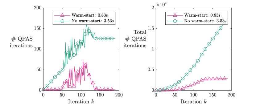
Figure 3: The figure shows the number of inner QPAS iterations required to reach optimality for a given subspace size. When we use warm-starting where the working set of the previous optimal subspace is used as initial guess, the number of inner iterations is reduced.

3.2 Factorisation update

3.2.1 Solving the linear system in QPAS with QR

In the QPAS algorithm (see algorithm 4), a system of equation is solved each iteration to obtain the Lagrange multiplier $\lambda_{k}$. The linear system is

(37) $$\begin{pmatrix}G&C^{T}_{\mathcal{W}_{k}}\\ C_{\mathcal{W}_{k}}&0\end{pmatrix}\begin{pmatrix}x\\ \lambda\end{pmatrix}=\begin{pmatrix}f\\ 0\end{pmatrix}.$$

Where $G$ is the Hessian of the QP-problem to be solved, $f$ is the linear term and $C$ is the matrix representing the inequality constraints. $C_{\mathcal{W}_{k}}$ is the matrix containing rows of $C$ with indices from the set $\mathcal{W}$. Block elimination leads to the following linear system that needs to be solved, each iteration,

(38) $$C_{\mathcal{W}_{k}}G^{-1}C^{T}_{\mathcal{W}_{k}}.$$

Every iteration, the working set $\mathcal{W}_{k}$ is expanded, reduced by one index or remains unchanged. This then means that the QR-factorization of $\left(C_{\mathcal{W}_{k}}G^{-1}C^{T}_{\mathcal{W}_{k}}\right)$ can be easily expanded or reduced. There exist routines to efficiently add or remove rows and columns from a QR factorization, [5].

3.2.2 Cholesky

The only linear system that we need to solve is the projected Hessian $G=V_{k}^{T}A^{T}AV_{k}^{T}\in\mathbb{R}^{k\times k}$. Because of the positive definiteness, a natural choice for a factorization is the (lower) Cholesky decomposition. The lower Cholesky decomposition of some Hermitian, positive definite matrix $H$ is $LL^{T}$ with $L$ a lower triangular matrix. As mentioned before, $G$ would only lose positive definiteness once the columns of $V$ become linearly dependent (and we thus have a solution). When this factorization (or its update) fails, the algorithm can be terminated. This allows us to properly terminate in cases where the residual does not shrink below the tolerance (semi-convergence).

When the basis expands $H$ becomes larger. If $H$ is expanded as follows

(39) $$\tilde{H}=\begin{bmatrix}H&c\\ c^{T}&d\end{bmatrix},$$

with $c\in\mathbb{R}^{k}$ a column vector and $d\in\mathbb{R}$ a scalar. Then the Cholesky factorisation can be updated as follows:

(40) $$\tilde{L}=\begin{bmatrix}L&0\\ L_{21}&L_{22}\end{bmatrix}$$

with

(41a) $$L_{21} =(L^{-1}c)^{T}$$

(41b) $$L_{22} =d-L_{21}L_{21}^{T}$$

Algorithm 2 Update of lower Cholesky factorization

1:procedure cholesky_append($L$, $c$, $d$)

2:     $U_{12}\leftarrow L^{-1}c$ $\triangleright$ Forward substitution

3:     $L\leftarrow\begin{bmatrix}L&0\\ U_{12}^{T}&\sqrt{d-U_{12}^{T}U_{12}}\end{bmatrix}$

4:     return $L$

5:end procedure

Remark 3.1.

The forward substitution in line 2 in 2 can be started before the Cholesky update has completed.

3.3 Limiting the inner iterations

In the early iterations it is often better to expand the basis first and then find the optimal coefficients. Indeed, a small basis cannot fully represent the solution and finding the optimal solution within this subspace is premature. An alternative is to limit the number of inner iterations and calculate the residual when this maximum is reached. In principle, we only require optimality at the final subspace. Limiting the number of inner iterations requires care. If we stop the inner iteration without feasibility then the orthogonality between the residuals is lost.

As can be seen in figure 4 that shows the number of inner iterations required to find the optimal solution for subspace $V_{k}$, there is a sweet spot for what the maximal number of inner iterations should be. If the number of inner iterations is high, we find the optimal solution in each intermediate subspace and we converge in the fewest number of outer iterations. However, each outer iteration takes longer because of the large number of inner iterations. Especially at the halfway point, it appears to be not useful to solve the projected problem exactly. An approximate (feasible) solution is sufficient up to a point. If the number of inner iterations is limited harshly, additional basis vectors are needed in the outer iterations leading to a larger subspace. This then has the effect of taking longer to converge. The sweet spot, in this example, seems to be 5 inner iterations, where we almost get a 33% speed-up.

Note that there is no effect on the orthogonality of the residuals if we stop with a feasible solution. This can be guaranteed if we stop the inner QPAS iterations when the maximum number of inner iteration is reached and $p=0$.

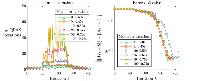
Figure 4: Limiting the number of inner iterations has little effect on the convergence but a big effect on the time to solution. At the left we show the number of inner iteration for various choices of maxit for the inner iteration. Note that we need to stop at an iteration wher $p=0$ to obtain feasibility to guarantee orthogonality. On the right we show the effect on the convergence. The time to solution is shown for each choice of inner iterations.

The final algorithm, with all improvements is written down in algorithms 3 and 4

Algorithm 3 Outer loop

1:procedure ResQPASS($A$, $b$, $l$, $u$, $\epsilon_{1}$, $\epsilon_{2}$, maxit)

2:     $r_{0}=-A^{T}b$

3:     $V_{1}=\begin{bmatrix}r_{0}/\|r_{0}\|\end{bmatrix}$

4:     $L=$ lower_cholesky($V_{1}^{T}A^{T}AV_{1}$)

5:     $\mathcal{W}_{0}=\emptyset$

6:     $y_{0}=[]$

7:     for $i=1,2,\ldots$ do

8:         $\left[y_{i},\mathcal{W}_{i},[\lambda_{i};\mu_{i}]\right]\leftarrow$

9:                 qpas($L,-b^{T}AV_{i},[-V^{T},V^{T}]^{T},[l^{T},u^{T}]^{T},[y_{i-1}^{T},0]^{T},\mathcal{W}_{i-1}$, maxit)

10:         $r_{i}=A^{T}(AV_{i}y_{i}-b)-\lambda_{i}+\mu_{i}$

11:         $v_{i+1}=r_{i}/\|r_{i}\|$

12:         $V_{i+1}=\begin{bmatrix}V_{i}&v_{i+1}\end{bmatrix}$

13:         if $\|r_{i}\|<\epsilon_{1}$ then

14:              return $V_{i}y_{i}$

15:         end if

16:         $c\leftarrow V_{i}^{T}A^{T}Av_{i+1}$

17:         $d\leftarrow v_{i+1}^{T}A^{T}Av_{i+1}$

18:         $L\leftarrow$ cholesky_append($L,c,d$) using algorithm 2

19:         if $|L|<\epsilon_{2}$ then$\triangleright$ $V_{i}^{T}A^{T}AV_{i}$ no longer pos. def.

20:              return $V_{i}y_{i}$

21:         end if

22:     end for

23:end procedure

Algorithm 4 QPAS with Cholesky factor and QR updates

1:procedure qpas($L,f,C,d,x_{0},\mathcal{W}_{0},\tt{maxit}$)

2:      $G^{-1}f\leftarrow$ Solve: $LL^{T}x=f$ $\triangleright$ Forward- and backward substitution

3:     for $k=0,1,2\ldots$ do

4:         Compute $p_{k},\lambda_{k}$ and helper variables for equality constrained subproblem:

5:         if $|\mathcal{W}_{k}|=0$ then

6:              $p_{k}\leftarrow-(x_{k}+G^{-1}f)$

7:              $\lambda,G^{-1}C^{T}_{\mathcal{W}_{k}},q\leftarrow\emptyset$

8:         else

9:              if $k=1$ then $\triangleright$ Warm-start

10:                  $G^{-1}C^{T}_{\mathcal{W}_{k}}\leftarrow$ Solve: $LL^{T}x=C^{T}_{\mathcal{W}_{k}}$

11:                  $[Q,R]\leftarrow\textsc{qr}\left(C_{\mathcal{W}_{k}}\left(G^{-1}C^{T}_{\mathcal{W}_{k}}\right)\right)$

12:                  $q\leftarrow-C_{\mathcal{W}_{k}}\left(x_{k}+G^{-1}f\right)$

13:              end if

14:              $\lambda_{k}\leftarrow$ Solve: $Rx=Q^{T}q$

15:              $p_{k}\leftarrow-\left(x_{k}\left(G^{-1}f\right)+\left(G^{-1}C^{T}_{\mathcal{W}_{k}}\lambda\right)\right)$

16:         end if

17:         Compute $x_{k+1}$ and update the working set $\mathcal{W}_{k+1}$:

18:         if $p_{k}=0$ then $\triangleright$ Optimum reached or unnecessary bound

19:              if $\forall i\in\mathcal{W}_{k}\cap\mathcal{I}:(\lambda_{k})_{i}\geq 0\textbf{ or }k\geq\tt{maxit}$ then

20:                  return $[x_{k},\mathcal{W}_{k},\lambda_{k}]$

21:              else

22:                  $j\leftarrow\operatorname*{argmin}_{j\in\mathcal{W}_{k}\cap\mathcal{I}}\lambda_{j}$

23:                  $\mathcal{W}_{k+1}\leftarrow\mathcal{W}_{k}\setminus\{j\}$

24:                  $G^{-1}C^{T}_{\mathcal{W}_{k+1}}\leftarrow$ remove column $j$ in $G^{-1}C^{T}_{\mathcal{W}_{k}}$

25:                  $[Q,R]\leftarrow$ Update QR factorisation,

26:                               with column, $j$ and row $j$ removed

27:                  $q\leftarrow$ Remove $q_{j}$ from $q$

28:                  $x_{k+1}\leftarrow x_{k}$

29:              end if

30:         else$\triangleright$ $\exists$ blocking constraint

31:              $\alpha_{k}\leftarrow\min\left(1,\min_{i\not\in\mathcal{W}_{k},\ C_{i}p_{k}<0}\frac{d_{i}-C_{i}x_{k}}{C_{i}p_{k}}\right)$

32:              $x_{k+1}\leftarrow x_{k}+\alpha_{k}p_{k}$

33:              if $\exists j\in\mathcal{I}$ blocking constraint then

34:                  $\mathcal{W}_{k+1}\leftarrow\mathcal{W}_{k}\cup\{j\}$

35:                  $G^{-1}C^{T}_{\mathcal{W}_{k+1}}\leftarrow\begin{pmatrix}G^{-1}C^{T}_{\mathcal{W}_{k}}&x\end{pmatrix}$ with $x:LL^{T}x=C^{T}_{j}$

36:                  $[Q,R]\leftarrow$ Update QR factorisation,

37:                               with column $C_{\mathcal{W}_{k}}x$ and row $C_{j}\left(G^{-1}C^{T}_{\mathcal{W}_{k+1}}\right)$ added

38:              else

39:                  $\mathcal{W}_{k+1}\leftarrow\mathcal{W}_{k}$

40:              end if

41:         end if

42:     end for

43:end procedure

3.4 Stability of QPAS

When a nonzero step $p$ is computed, a stepsize $\alpha_{k}$ is determined. The definition of $\alpha_{k}$ can be found in line 31 in 31, $C_{i}$ is the $i$-th row of matrix $C$. Two matrix vector products are computed in this step: $Cx_{k}$ and $Cp_{k}$. However, the definition of $x_{k+1}=x_{k}+\alpha_{k}p_{k}$ implies the possibility of a recursive relationship for $Cx_{k+1}$:

(42) $$Cx_{k+1}=Cx_{k}+\alpha_{k}Cp_{k}.$$

where $Cp_{k}$ was already computed to find $\alpha_{k}$. We expect this recursion to reduces runtime. This doesn’t cause instability in our experiment.

In figure 5 we compare the recursive case with 5 and 10 inner iterations to the direct case for a problem from example 2.10 with $A\in\mathbb{R}^{10,000\times 6,000}$ and $m_{\max}=256$. The norm of the recursion error is also shown. The direct method is the slowest, as expected. The case with 10 inner iterations behaves exactly the same as the direct case, only 5% faster. The case with 5 inner iterations is slightly slower because of the delayed convergence caused by the stringent bound on inner iterations. It is however still faster than the direct method.

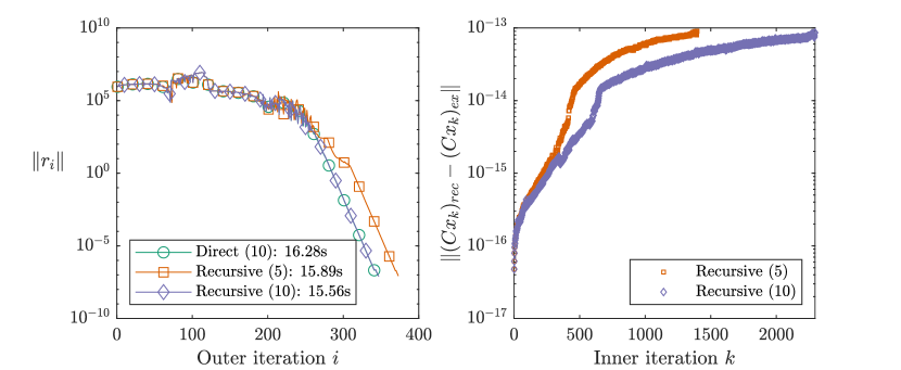
Figure 5: Comparison between the recursive version with 5 and 10 inner iterations and the direct version.

Note that a similar recurrence is used in CG for the residual. It also avoids a sparse-matrix multiplication and its effect on the rounding error is well studied, see for example Chapter 5 in [10].

4 Numerical experiments

The paper is accademic in nature and mainly explores the possibilities that projections and Krylov-like methods still offer. Therefore the problems are synthetic for now, to show that ResQPASS is promissing. Detailed error analysis and final attainable accuracy are future work along with in depth studies of specialised applications.

4.1 Conjugate Gradients (CG)

As mentioned in example 2.9, the unconstrained ResQPASS applied to $\|Ax-b\|$ converges like CG applied to $A^{T}Ax=A^{T}b$. For this experiment, the entries of $A\in\mathbb{R}^{m\times n}$ and $x_{ex}\in\mathbb{R}^{n}$ are drawn from a normal distribution with mean 0 and standard deviation 1 and all values smaller than 0 and bigger than 0.1 are set to 0. This gives us a sparse $A$ with $3.98\%$ fill. The right hand side is defined as $b=Ax_{ex}$. For our experiment we look at overdetermined and underdetermined systems with an aspect ratio of 10:6. The matrix $A^{T}A$ is close to a full matrix, especially for big $A$. In figure 6 we can see that ResQPASS is still able to exploit the sparsity. If we perform dense matrix-vector multiplication, the performance of ResQPASS and CG is similar for the overdetermined case, but ResQPASS is faster in the underdetermined case. CG can be sped up in this case by not computing $A^{T}A$ explicitly and performing the dense matrix-vector product $(A^{T}A)p$. Instead, we perform two sparse multiplications $A^{T}(Ap)$. In this case ResQPASS performs similarly but with a slight overhead.

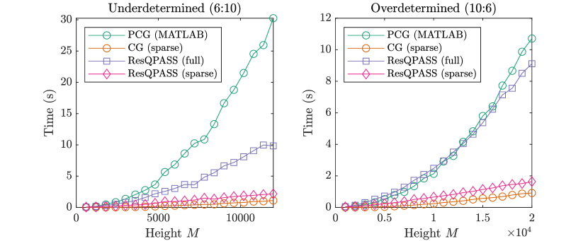
Figure 6: Comparison in runtime for varying sizes of $A$ between ResQPASS (with dense and sparse matrix multiplication) MATLAB’s CG implementation pcg and an improved version of CG that still exploits sparse matrix multiplication.

4.2 Bounded Variable Least Squares (BVLS)

In this experiment, we use the formulation of example 2.10 with $A\in\mathbb{R}^{10,000\times 6,000}$. First of all, the numerical improvements done to the QPAS method give already a significant advantage compared to MATLAB’s active-set based solver and a naive QPAS implementation. Projection still seems beneficial, as ResQPASS is faster than the improved QPAS. In figure 7 it is also clear that for this problem with a small number of active constraints, ResQPASS outperforms IP. For sufficiently large $m_{\max}$ ResQPASS would however cross over IP (like MATLAB’s QPAS does). This is because the runtime of interior-point (IP) methods is known to be independent of the number of active constraints, whereas for ResQPASS (and other active-set algorithms) it does depend on the number of active constraints [14].

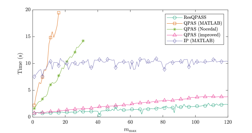
Figure 7: Comparison in runtime between ResQPASS, MATLAB’s QPAS implementation, the basic QPAS implementation mentioned in [14], algorithm 4 and MATLAB’s interior point implementation for different $m_{\max}$.

4.3 Nonnegative Matrix Factorisation (NMF)

The $n\times m$ matrix $A$ is given and we look for the unknown $U\in\mathbb{R}^{n\times p}$ and $V\in\mathbb{R}^{p\times m}$, with $X,Y\geq 0$ (elementwise), such that $\|A-XY\|$ is minimal. This can be achieved with the Alternating Least Squares (ALS) algorithm [7]. In the ALS algorithm nonnegative least squares problems need to be solved, for which ResQPASS could be used. As mentioned in remark 2.2 the problem should be translated such that 0 is feasible.

Let the function $\operatorname{vec}(X)$ be the vectorization of the matrix $X$, where columns are stacked. We can rewrite $\|A-UV\|^{2}$ as $\|\operatorname{vec}(A)-(I_{m}\otimes U)\operatorname{vec}(V)\|^{2}$ and $\|\operatorname{vec}(A)-(V^{T}\otimes I_{n})\operatorname{vec}(U)\|^{2}$ to get a classical least squares formulation.

Algorithm 5 NMF with ALS

1:procedure ALS(A,p)

2:     $U=\text{rand}(n,p)$

3:     for $i\in\{1,\ldots,10\}$ do

4:         $V={\displaystyle\operatorname*{argmin}_{V\geq 0}}\frac{1}{2}\|A-UV\|^{2}$

5:         $U={\displaystyle\operatorname*{argmin}_{U\geq 0}}\frac{1}{2}\|A-UV\|^{2}$

6:     end for

7:end procedure

We use the synthetic example of [4] where the matrix $A$ is constructed as follows. $X,Y$ are $n\times p$ and $p\times m$ matrices respectively, with uniformly drawn random entries between 0 and 1. Gaussian noise with mean 0 and standard deviation 0.1 is added to the product $XY$ and all negative values are set to 0 to obtain $A$.

The number of ALS iterations is fixed to 10 (20 minimizations) and the maximum number of inner QPAS iterations for ResQPASS is set to 10. In figure 8 we can see that ResQPASS has a big speed advantage (one or two orders of magnitude), without sacrifying accuracy of the solution.

Figure 8: Comparison between ALS implemented with either MATLAB’s nonnegative least squares (lsqnonneg) or ResQPASS for varrying sizes and 10 iterations

4.4 Contact problem

In contact problems the freedom of the solution is limited due to spatial limitations. These bounds limit the solution space and we require a subspace that is adapted to these circumstances. We study the convergence of a cartoon model for an inflated balloon with limited space for inflation. In a balloon the elastic forces are balanced by the pressure inside the balloon. This leads to a equilibrium between the curvature and the magnitude of the pressure. So the Laplacian applied to the solution is equal to the pressure vector, which is constant through the domain. This leads to a system of equations $Lx=p$, where $L\in\mathbb{R}^{n\times n}$ is the Laplacian, $x\in\mathbb{R}^{n}$ is the solution that models the surface deformation of the balloon, $p\in\mathbb{R}^{n}$ is the pressure vector.

However, if the solution is limited by lower and upper bounds, this results in a bounded variables QP problem. In this case we minimize the energy with bounds on the solution. This is

(43) $$\|Lx-p\|^{2}_{2}$$

$$l\leq x\leq u$$

For the cartoon example, we are using $l=0$ and $u=0.1$ and a constant pressure vector. The domain is $[0,1]^{2}$.

The matrix is the 3-point stencil approximation of the Laplacian. The matrix can be written as $A_{\text{2D}}=A_{1D}\otimes I+I\otimes A_{1D}$, where $A_{1D}$ is the 1D finite-difference Laplacian matrix, a tridiagonal matrix with constant diagonals. We use a mesh with 50x50 grid points and a pressure vector with a constant value of 4.

In figure 10 we show the convergence of the ResQPASS method for the contact problem, both for the preconditioned and the unpreconditioned problem. The corresponding solutions after 200 iterations are shown in figure 9.

The preconditioning matrix is based on the incomplete LU factorisation of the Hessian $A^{T}A$. We use a threshold of 0.1 for the ilut factorisation. Instead of using the residual (5) we use a preconditioned residual, solution of

(44) $$Mr_{k}=A^{T}(AV_{k}y_{k}-b)-\lambda_{k}+\mu_{k},$$

where $M=LU$ is built out of the incomplete factorisation. When none of the bounds are active this corresponds to the ILU preconditioned CG.

The unpreconditioned iteration does not reach the bounds in the first 200 iterations. It follows the CG convergence. However, for the preconditioned solution we reach the bounds after 15 iterations. From then on the subspace is adapted to the bounds. We see that the solution is adapted to these bounds, see left hand side of figure 9.

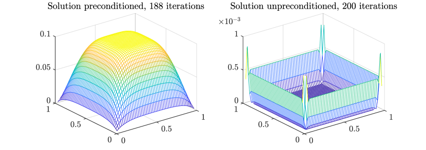
Figure 9: Solution after 200 iterations for the preconditioned and unpreconditioned problem. The unpreconditioned iteration converges very slowly and has not reached the bounds by iteration 200. However, the preconditioned iteration reaches the bounds starting from iteration 15. As explained earlier, the residuals that are used as a basis then start to include effects from the Lagrange multipliers and the solution adapts to the bounds. The preconditioned version reaches the desired tolerance before the maximum number of iterations is reached.

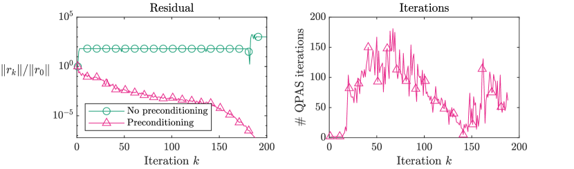
Figure 10: Left: The convergence for the contact problem (43) for the ResQPASS algorithm, both for preconditioned and unpreconditioned problem. We precondition the iteration using the incomplete LU factorisation of $A^{T}A$. This significantly accelerates the convergence of the problem.
Right: We show the number of inner QPAS iterations for the preconditioned problem. The first few iterations no bounds are reached, hence no inner iterations are required. But then as the bound become active a significant number of inner iterations is used. Because of the preconditioning, the solution can significantly change from one solution to the next, hence the significant number of inner iterations.

5 Discussion and conclusion

In this paper we present the Residual QPAS subspace method (ResQPASS). The method solves box-constrained linear least squa-res problems with a sparse matrix, where the variables can take values between a lower and an upper bound. In this paper we have proposed the subspace method, analysed the convergence and documented how it is efficiently implemented. It uses warm-starting and updates the factorisation.

Similar as in Krylov methods the sequence of residual vectors are pairwise orthogonal. The residual vectors that we use include the current guess for the Lagrange multipliers. The inner problem only needs to be solved for feasibility to obtain an orthogonal basis.

The ResQPASS works fast if the vector of Lagrange multipliers is sparse, i.e. when only a few of the box constraints are active and most Lagrange multipliers are zero. As soon as the active set is discovered, Krylov convergence sets in. We then converge fast to the solution. As in classical Krylov methods, when you restart, it is hard to benefit from superlinear convergence.

Note that it is possible to further accelerate the Krylov convergence with the help of a preconditioner. We then use residuals that are the solution of $Mr_{k}=A^{T}(Ax_{k}-b)-\lambda_{k}+\mu_{k}$ for some non-singular matrix $M$ that is cheap to invert. The residuals are then $M$-orthogonal.

However, there are many inverse problems where many unknowns hit the boundary. For example, a deblurring of a satellite picture against a black background. In that case the Lagrange multipliers are not sparse. However, the deviation from the bounds in $x$ is sparse, hence a dual ResQPASS algorithm might be applicable. Initial experiments confirm this intuition and the dual algorithm exhibits similar superlinear convergence. The analysis of the dual algorithm is the subject of a next paper.

Other applications can be found in contact problems in mechanics, where the subproblems touch each other in only a few places. These points of contact are often unknown upfront.

Other future work is a thorough analysis of the propagation of rounding errors and effects of the loss of orthogonality.

References

- [1] G. Golub and W. Kahan, Calculating the singular values and pseudo-inverse of a matrix, Journal of the Society for Industrial and Applied Mathematics, Series B: Numerical Analysis, 2 (1965), pp. 205–224.
- [2] G. H. Golub, P. C. Hansen, and D. P. O’Leary, Tikhonov regularization and total least squares, SIAM journal on matrix analysis and applications, 21 (1999), pp. 185–194.
- [3] J. Gondzio, Interior point methods 25 years later, European Journal of Operational Research, 218 (2012), pp. 587–601.
- [4] R. Gu, S. J. Billinge, and Q. Du, A fast two-stage algorithm for non-negative matrix factorization in smoothly varying data, Acta Crystallographica Section A: Foundations and Advances, 79 (2023).
- [5] S. Hammarling and C. Lucas, Updating the QR factorization and the least squares problem, (2008).
- [6] P. C. Hansen, J. G. Nagy, and D. P. O’leary, Deblurring images: matrices, spectra, and filtering, SIAM, 2006.
- [7] T. Hastie, R. Mazumder, J. D. Lee, and R. Zadeh, Matrix completion and low-rank SVD via fast alternating least squares, The Journal of Machine Learning Research, 16 (2015), pp. 3367–3402.
- [8] A. C. Kak and M. Slaney, Principles of computerized tomographic imaging, SIAM, 2001.
- [9] C. L. Lawson and R. J. Hanson, Solving least squares problems, SIAM, 1995.
- [10] J. Liesen and Z. Strakos, Krylov subspace methods: principles and analysis, Oxford University Press, 2013.
- [11] M. E. Lübbecke and J. Desrosiers, Selected topics in column generation, Operations research, 53 (2005), pp. 1007–1023.
- [12] V. A. Morozov, Methods for solving incorrectly posed problems, Springer Science & Business Media, 2012.
- [13] J. G. Nagy and Z. Strakos, Enforcing nonnegativity in image reconstruction algorithms, in Mathematical Modeling, Estimation, and Imaging, vol. 4121, SPIE, 2000, pp. 182–190.
- [14] J. Nocedal and S. J. Wright, Numerical optimization, Springer, 1999.
- [15] Y. Saad, Iterative methods for sparse linear systems, SIAM, 2003.
- [16] P. B. Stark and R. L. Parker, Bounded-variable least-squares: an algorithm and applications, Computational Statistics, 10 (1995), pp. 129–129.
- [17] R. Tibshirani, Regression shrinkage and selection via the LASSO, Journal of the Royal Statistical Society: Series B (Methodological), 58 (1996), pp. 267–288.
- [18] H. A. Van der Vorst, Iterative Krylov methods for large linear systems, no. 13, Cambridge University Press, 2003.
- [19] W. Vanroose and J. Cornelis, Krylov-simplex method that minimizes the residual in -norm or -norm, arXiv preprint arXiv:2101.11416, (2021).
- [20] H. Zou and T. Hastie, Regularization and variable selection via the elastic net, Journal of the royal statistical society: series B (statistical methodology), 67 (2005), pp. 301–320.