Parametric dependence between random vectors via copula-based divergence measures
Steven De Keyser, Irène Gijbels
Abstract. This article proposes copula-based dependence quantification between multiple groups of random variables of possibly different sizes via the family of -divergences. An axiomatic framework for this purpose is provided, after which we focus on the absolutely continuous setting assuming copula densities exist. We consider parametric and semi-parametric frameworks, discuss estimation procedures, and report on asymptotic properties of the proposed estimators. In particular, we first concentrate on a Gaussian copula approach yielding explicit and attractive dependence coefficients for specific choices of , which are more amenable for estimation. Next, general parametric copula families are considered, with special attention to nested Archimedean copulas, being a natural choice for dependence modelling of random vectors. The results are illustrated by means of examples. Simulations and a real-world application on financial data are provided as well.
The fundamental problem of measuring dependence between two random variables is customary in the analysis of bivariate data. Linear relationships are embodied in the Pearson correlation coefficient and concordance measures like Kendall’s tau or Spearman’s rho, among many others, extend to incorporate monotone dependence. The interest of generalizations of such concordance measures to more than two univariate random variables is also widely recognized, see e.g. Nelsen (1996), Schmid and Schmidt (2007) and Gijbels et al. (2021). Important is the compliance with certain postulated axioms, starting with Rényi (1959) and followed by e.g. Lancaster (1963), Schweizer and Wolff (1981) and Embrechts et al. (2002) for the case of two univariate random variables, and e.g. Wolff (1980), Nelsen (1996) and Gijbels et al. (2021) when the interest is in more than two variables.
Another extension consists of looking at two groups of random variables. In this context, one is typically aware of the statistical analysis of canonical correlations, as in Hotelling (1936). Grothe et al. (2014) suggest using concordance measures and Mordant and Segers (2022) measure dependence between two random vectors via optimal transport, making a Gaussian assumption when going to statistical inference. Often, dependence capturing is restricted to monotone relationships, either due to making rather stringent assumptions (e.g. Gaussianity), or because the measures in question have limited detection ability (e.g. concordance measures do not measure tail dependence).
De Keyser and Gijbels (2023) work in the broader setting of random vectors, think of e.g. answers to different questionnaires or groups of financial assets like shares from different stock indexes, and define the general family of -dependence measures, which complies with their postulated properties that are driven by the objective of quantifying any deviation from independence. In this article, we elaborate more on these dependence measures. After proving several desirable properties, we focus on some examples of maximal dependence in singular copula distributions. Thereafter, we assume absolute continuity and concentrate on parametric and semi-parametric modelling and estimation from a copula density point of view.
Unlike numerous dependence measures (concordance measures, tail dependence coefficients, -copula distances like the Hoeffding’s of Geißer et al. (2010), ) inquiring about the (bounded) copula cdf, we now have functionals of the density. Copula densities may have rather cumbersome mathematical expressions, but numerical approximations are at hand if the dependence coefficient has no explicit analytical form in terms of the copula parameters. We also take extra care at boundaries, where copula densities commonly tend to infinity or zero.
The family of -dependence measures includes many popular measures that have a strong ability to detect deviations from independence, and there exists a great deal of statistics providing inference procedures and pursuing practical usefulness. The outline of this paper is the following.
Section 2 discusses possible axioms for dependence measures in the general context of random vectors, and they are verified for the proposed dependence measures is Section 3. A Gaussian copula approach and corresponding statistical inference is considered in Section 4, after which general parametric copulas are dealt with in Section 5, where the focus will be on maximum likelihood estimation. Some simulation studies are presented in Section 6, and a real life application to financial data is to be found in Section 7. We end this paper with a brief discussion in Section 8. For proofs related to the asymptotic properties of the proposed estimators (Theorems 1 and 2), we refer to the Appendix.
2. Notation and axioms
The general setting is the same is in De Keyser and Gijbels (2023), i.e. we consider a -dimensional random vector having marginal random vectors for composed of marginal univariate random variables for , with , which are assumed to be continuous. The interest is in dependence measures . We have continuous marginal cdf’s, say , of for and . Sklar’s theorem (Sklar (1959)) guarantees the existence of a unique (-dimensional) copula of and marginal (-dimensional) copulas of for . They bring forth respective probability measures and . Plausible axioms for a valid dependence measure are as follows.
(A1)
For every permutation of : ; and for every permutation of , for , it holds:
.
(A2)
.
(A3)
if and only if are mutually independent.
(A4)
with equality if and only if is independent of .
(A5)
is well defined for any -dimensional random vector and is a functional of solely the copula of .
(A6)
Let for and be strictly increasing, continuous transformations. Then
where for .
(A7)
Let be a strictly decreasing, continuous transformation for a fixed and a fixed . Then
where .
(A8)
Let be a sequence of -dimensional random vectors having copulas , then
if uniformly, where denotes the copula of .
We now bring forward the family of -dependence measures and show its compliance with the above properties. For (A8), we will restrict ourselves to uniform convergence of the copula densities.
3. -dependence measures
Write for the Lebesgue decomposition of with respect to the product measure , i.e.
is absolutely continuous with respect to (denoted as ) and is singular with respect to (denoted as ).
3.1. Definition and properties
The family of -dependence measures between random vectors is defined in De Keyser and Gijbels (2023) as follows.
Definition 1. (-dependence measures)
Consider a continuous, convex function with . Extend by defining
The -dependence between is the quantity defined by
with the set on which is concentrated.
We use the convention .
The maximum value of is , and attained when . After looking at some examples of maximal -dependence in singular copulas, we restrict ourselves in this paper to with the Lebesgue measure (hence, and ), implying that
(1)
,
where , and the copula densities (w.r.t. and ) corresponding to and for and with for . Before showing compliance of the -dependence measures with our stated axioms, we define an artificial normalization to be a continuous, strictly increasing mapping satisfying and . As an example, Joe (1989) suggests in case , because then the normalized dependence coefficient reduces to in case of a bivariate Gaussian distribution with correlation .
Proposition 1.Let be defined by (1) and normalized to
where is an artificial normalization as explained above. Then, satisfies (A1),(A2),(A5),(A6) and (A7). If is strictly convex at , property (A3) is satisfied, and (A4) holds if is strictly convex on . Axiom (A8) is fulfilled if we replace and by the existing densities and , and when is uniformly bounded from below and above by a strictly positive constant.
Proof.
Property (A1) holds because of Fubini’s theorem and knowing that permuting the components of a random vector, results in permuting the copula components accordingly. The results stated about (A2) and (A3) follow from Theorem 1 of De Keyser and Gijbels (2023) and applying the normalization.
For Property (A4), suppose that has copula density with marginal copula density of . Put Then,
where we used Jensen’s inequality. If is independent from , we have and the equality holds. If is strictly convex, the equality holds if and only if
, where is a function of not depending on almost surely for almost every . Integrating this equality with respect to gives , i.e. .
Obviously, by definition, Property (A5) and hence also (A6) are fulfilled. Next, in the context of Property (A7), assume without loss of generality that gets transformed to for a strictly decreasing transformation and let be the copula density of with . Then, with and with the copula density of . Hence,
by simply doing a substitution .
Finally, given there exist such that for all , and uniformly on , some basic analysis implies that
uniformly on as , where are the marginal copula densities of for . Property (A8) in terms of copula densities is then satisfied by the Lebesgue dominated convergence theorem.
∎
Remark 1.
For showing (A3), we assumed that is strictly convex at . While convexity is usually defined as a global property of a function, we use Definition 1 of local strict convexity of Liese and Vajda (2006), i.e. is strictly convex at if it is convex and not locally linear at .
Remark 2.
Consistency results for dependence measures based on the copula cdf are typically based on the weak uniform convergence of the empirical copula process. In copula density terms, the stated conditions in Proposition 1 for fulfilling (A8) are rather stringent. Indeed, it is known that many of the common copula families (e.g. normal, Student, Clayton, Gumbel) have densities that explode to infinity near some boundaries points, see e.g. Omelka et al. (2009). This means that consistency arguments relying on uniform convergence are typically limited to compact subsets of . However, there are theoretical properties that favour copula density based dependence measures, see Remark 3.
Remark 3.
When using a dependence measure that compares the true copula cdf to the one under independence, like the Hoeffding’s of Geißer et al. (2010) (with ) using the -distance, the independence characterization Axiom (A3) is still satisfied, but stays rather ambiguous. The reason is that such dependence measures can be made arbitrarily small, while maintaining an exact deterministic relationship (singularity) between all the variables. An explicit proof of this follows from Theorem 3.2.2 of Nelsen (2006), telling us that we can approximate the independence copula arbitrarily and uniformly closely by copulas (shuffles of Min) exhibiting a perfect deterministic relationship (‘complete dependence’ in the sense of Lancaster (1963)). The copula density based -dependence measures are more alert to such singularities.
It is also interesting to think about the meaning of maximal -dependence. Such maximal dependence occurs if there is a certain singularity (and hence the copula density does not exist everywhere). First, we give an overview of popular choices for , the corresponding name, and its maximum value , see Table 1.
Note that all the -functions in Table 1 are strictly convex on , except for the total variation distance, which is only strictly convex at . The mutual information is a prominent quantity in information theory, see e.g. Cover and Thomas (2006). Differential Shannon entropy quantifies the average amount of uncertainty and mutual information equals
the difference between the differential entropy under independence and under the true model. A general family is with , for which and for (for , this is the total variation distance).
We refer to Liese and Vajda (2006) and references therein for further statistical applications, as well as for other choices of . For the Jensen-Shannon divergence, we refer to Österreicher and Vajda (2003).
Name
mutual information
Pearson distance
Hellinger distance
total variation distance
Jensen-Shannon distance
Table 1: Common choices for the function .
3.2. Perfect dependence
Next to independence, there is some kind of maximal dependence at the opposite end of the spectrum, to which we will refer as perfect dependence. Perfect dependence is inherent to the dependence measure and occurs if and only if the measure in question reaches its maximum value.
Two random variables are often seen as maximally dependent if their copula is the Fréchet upper or lower bound copula, that is if almost surely, with the cdf of for , or if almost surely. In this case, concordance measures like Kendall’s tau and Spearman’s rho are maximal. This however focuses on monotonic dependence, and perfect co- or counter-monotonicity are only particular cases of ‘strict dependence’ as in Rényi (1959), telling that for some function , or for some function (deterministic predictability of one variable through the other). When (or ) is invertible, we get the ‘complete dependence’ of Lancaster (1963).
More general is the ‘pure dependence’ of Geenens and Lafaye de Micheaux (2022), being the existence of a function such that for a certain , and with , where is the image of under . We provide an example of pure dependence.
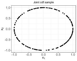
Example 1. Consider (equality in distribution) with
(2)
and interconnected by the copula
(3)
where is the indicator function. Figure 1 shows scatter plots of and based on a random sample of size . This is clearly an example of pure dependence, with function given by . Note however that this is not an example of strict dependence nor of complete dependence.
We can easily extent this notion of pure dependence to random variables , and formulate it in terms of , as the existence of a such that for certain , and with . The intuition associated with pure dependence is akin to understanding perfect dependence inherent in the -dependence measures.
Figure 1: Scatter plot (sample size ) of bivariate copula (3) (left) and cdf (right) when (2) are the marginals.
Theorem 1 of De Keyser and Gijbels (2023) suggests that perfect -dependence ( maximal) between random vectors arises when there exists a such that and (i.e. , hence , where is the Borel sigma-algebra on . Restricting to -functions that are strictly convex at , and satisfy , this is the only case in which is maximal (and hence we obtain a characterization of perfect dependence). We illustrate this singularity between random vectors by means of another example.
Example 2. Consider having copula
for . Then and have a Gumbel copula and and the comonotonicity copula. We have , since is concentrated on . Also, , since ( the copula of and the copula of .
On the other hand, we have since
and (now defining as the copula of and as the copula of ). In fact, this is an example of , , but .
In Example 6, we illustrate that (for one particular choice of ) is actually nothing more than of a two dimensional Gumbel copula, which is pretty intuitive, since and both have the comonotonicity copula and thus and can be seen as one, as well as and , and (just as ) has a Gumbel copula.
In short, -dependence is maximal when there is a singularity among random variables belonging to different random vectors, indifferent to plausible singularities between random variables within one and the same random vector.
4. A Gaussian copula approach
In this section, we assume a Gaussian copula model for . Although a restricted framework, it leads to interesting statistical inference results. In fact, we only assume finite second moments and the existence of the covariance matrix of , say
where contains the covariances between the components of and for , and the within covariances of for . If has a normal distribution, a straightforward calculation shows that (1) reduces to
(4)
with
the covariance matrix under mutual independence of , and . In (4), we used a superscript referring to the Gaussian assumption and emphasize the dependence on merely the covariance matrix . For certain specific choices of the function , the above integral allows a closed form solution in terms of the covariance matrix . We shall go deeper into the cases and , and denote the resulting dependence measures as and (for the other choices of listed in Table 1, there is no such elegant closed form solution to (4)). It is a straightforward calculation to show that
(5)
and, denoting for the identity matrix,
(6)
It is also easily checked that, if and , i.e. in the case of two univariate random variables, the expression (6) reduces to what was found in Section 4 of Geenens and Lafaye de Micheaux (2022).
Notice that (5) and (6) are formulated in terms of covariance matrices. However, since our dependence measures are copula-based, they should be scale-invariant. Let be the diagonal matrix with the variances on the diagonal. Then, the correlation matrix corresponding to satisfies , such that is just a rescaling of by multiplying the latter with the product of all variances. From this, we easily see that . Moreover,
with the correlation matrix corresponding to , implying that . For general , we obtain this relation by performing the substitution in (4).
Also, since we do not care about univariate marginals, needs not to be the traditional Pearson correlation matrix of a multivariate normal distribution, but can be the margin free Gaussian copula correlation matrix of normal scores, that is
(7)
for , and , where Corr stands for the traditional Pearson correlation, and for the standard normal quantile function.
Statistical inference
Based on a sample for from , with for a sample from for , the sample version of (7) is known as the matrix of normal scores rank correlation coefficients (Hájek and Šidák (1967)),
(8)
defined through normal scores
obtained from the univariate empirical cdf for and .
The quantity is computed as the conventional Pearson correlation of the bivariate sample of scores and by noting that
which follows from the fact that for and is the rank of in the sample . Being rank-based, makes the variance of the normal scores independent of the data.
A next natural step in estimating is to just plug in instead of the unknown matrix . Let be the set of all covariance matrices and the set of all positive definite ones. Let be the map defined by for , and the Frobenius matrix norm, i.e. . If we can show the Fréchet differentiability of the mapping
(9)
on , then the delta method turns an asymptotic normality result for into an asymptotic normality result for . For general , interchanging Fréchet differentiation and Lebesgue integration in (4) would be useful, and holds if there exists an integrable function on dominating the Fréchet derivative of the integrand of (4) uniformly on . Here, special attention is again devoted to either or , because we have the more explicit expressions (5) and (6). Theorem 1 states formally the asymptotic normality result for .
Theorem 1.Let have a Gaussian copula with correlation matrix , and let be given by (8), based on which the plug-in estimator is constructed. If the mapping defined in (9) is Fréchet differentiable, then the estimator is asymptotically normal. Moreover, if differentiation and integration in (4) can be interchanged, we have in addition the expression for the asymptotic variance:
with asymptotic variance
where is the diagonal matrix consisting of the diagonal of , and with
defining , , and
for
In particular, one can show that
and
defining
The expression for in Theorem 1 was obtained in the proof using the explicit formula (5) that we have for the mutual information (similarly for the Hellinger distance). In the following example, we verify, for , the general formula for relying on interchanging the Fréchet derivative and Lebesgue integral.
Example 3.
In case , the different terms in the general formula for , for a certain , can be calculated as follows. First, using (A1) in the proof of Theorem 1, we have
where
Next, observe that
Using , it is also straightforward to see that
and
and finally
Combining all this, we obtain that
where we used the following properties of quadratic forms
for certain compatible matrices , the cyclic trace property, and the fact that and . Hence, we have verified that the general formula for also brings us to
We end this section by looking at a specific four dimensional Gaussian copula family.
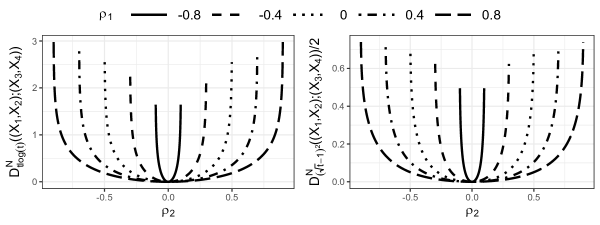
Example 4. Consider a four dimensional random vector having a Gaussian copula with correlation matrix
Then one can check that
(10)
and
(11)
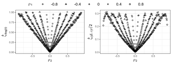
Figure 2: Mutual information (10) (left) and half Hellinger distance (11) (right) as a function of for different values of .
In (11), we normalized the Hellinger distance, guaranteeing a dependence measurement in (recall Proposition 1). For the mutual information, an artificial normalization is required, but we do not do not implement it here. Figure 2 shows how (10) and (11) depend on for different values of .
Some observations are:
•
iff .
•
For (singularity of and w.r.t. ), we must have and see that and .
•
If (absolute continuity of and w.r.t. , but singularity of w.r.t. ), we get and .
•
For (singularity of and w.r.t. ), , and , being the mutual information and half Hellinger distance of a bivariate Gaussian copula with correlation and is maximal iff .
Note that the principal components of are
and similarly, those of are
Moreover, , but
And so, we see that if , , i.e. the principal components and are perfectly correlated. This means that the four dimensional random vector is propagated in a three dimensional subspace (scatterplot of constitutes a hyperplane), resulting in the singularity of with respect to and explaining maximal dependence.
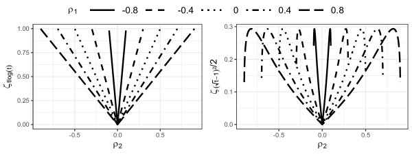
Figure 3: Asymptotic standard deviation of mutual information (left) and half Hellinger distance (right) as a function of for different values of .
Figure 3 shows the asymptotic standard deviation of the mutual information and of the half Hellinger distance (as in Theorem 1) as a function of for different values of , which can be calculated as
In general, we see that higher degrees of dependence come with higher asymptotic variance. For the Hellinger distance, however, the asymptotic variance goes down to zero when we get close to the previously discussed singularity, i.e. when gets close to satisfying . For instance, if , the asymptotic variance is maximal at , after which it converges to zero for . From its mathematical expression above, and its general form in Theorem 1, we see the factor in case of singularity makes the asymptotic variance of the Hellinger distance tend to zero.
5. A maximum likelihood approach
A Gaussian copula model is restricted to monotone dependence structures in terms of correlations. However, in many cases other relationships are present. Think for instance of comovements in the tails of stock returns. Thanks to Proposition 1 (in particular the fulfillment of Axiom (A3)), we know that -dependence measures are able to capture such associations as well. In practice, a sufficiently flexible estimation methodology is required. If one is willing to, for example, assume a Clayton copula model for two random variables and , we can use this assumption to estimate and hence, next to a monotone relationship, possible lower tail dependence is guaranteed to be incorporated as well.
5.1. Maximum likelihood-based inference
In general, in this section, we assume a specified parametric model for the copula density of , say , where . Notice that a Gaussian copula is also a parametric copula of this form when we stack all upper triangle elements of the correlation matrix in a vector. The univariate marginals for and are approached in either a parametric, or non-parametric way, leading to two different estimation procedures.
Case 1: parametric marginals.
A first option is to also assume a parametric statistical density model for , say . Based on a sample from , the full log-likelihood is
(12)
Let and be the MLE of , obtained by maximizing (12). It is a very well-known result that under certain regularity conditions (true lies in an open subset in which the log-density admits third derivatives w.r.t. the parameters that are uniformly bounded by an integrable function, and interchanging of derivatives and integral for score equations, see e.g. Theorem 4.1 on page 429 in Lehmann (1983)), one has
that is an asymptotically normal estimator.
If is -dimensional and all one dimensional, (12) is a -dimensional optimization problem. In case of a multivariate normal distribution, one has for the vector of upper triangle elements of the correlation matrix of the normal copula, and the mean and variance of .
Given estimators of (e.g. also based on MLE using the sample ), the pseudo log-likelihood for estimating is
If is -dimensional and all one dimensional, this is
an -dimensional optimization problem, after having done one dimensional optimization problems. This method is known as the inference functions for margins (IFM) method, and extensively studied in Section 10.1 of Joe (1997). Asymptotic normality is known to hold under the same regularity conditions as for the MLE.
For a multivariate normal distribution, it is known that .
Case 2: non-parametric marginals. If no appropriate parametric models can be proposed for the marginals, an option consists of estimating the marginals via the empirical cdf
and the copula parameter through maximizing
(13)
resulting in an estimator for . Again under the same regularity conditions, it is shown in Genest et al. (1995) that is asymptotically normal. If is the Gaussian copula density, there is no known expression for the maximizer of (13) over all correlation matrices, and numerical maximization is often used (see Section 5.5.3 in McNeil et al. (2005) for more details), being quite unfeasible in high dimensions. Of course, we have the results from Section 4 dealing with the Gaussian copula case.
In all the above cases, we have an asymptotically normal estimator for . A natural estimator for the copula density is then . If is unbounded, we will generally not have uniform consistency of (recall Remark 2). Nevertheless, Fréchet differentiability of the mapping
(14)
suffices to turn the asymptotic normality result of into an asymptotic normality result for the plug-in estimator . Still, the estimator would often require high-dimensional numerical integration, because usually the integral in (14) does not have a closed-form expression in terms of . That is why we suggest the following general approach.
Let be a user defined sample size for each , and with for , a sample from having distribution given that , that is
We then propose
(15)
as estimator for the -dependence given in (1). The rationale is that -dependence measures can be seen as an expectation and the empirical mean in (15) tries to approximate this integral. Since we have an explicit form of the estimated copula, we can take as many samples as we want when is given, and the larger , the better the approximation will be. It is intuitively clear (yet not trivial to prove) that, for large enough in some sense, the asymptotic properties of carry over to . A conditional law of large numbers will give substance to this, see Remark 4. Theorem 2 states the asymptotic normality result for .
Theorem 2.Let be an asymptotically normal estimator for based on which the estimator (15) is constructed, where the user chosen parameter is such that
for .
If the mapping defined in (14) is Fréchet differentiable, the estimator is asymptotically normal. Moreover, if the derivative can be moved into the integral, we have the expression for the asymptotic variance-covariance:
as , where is the asymptotic variance-covariance matrix of , and
defining , the ’th component of as , and
Remark 4. A conditional version of Kolmogorov’s law of large numbers (see Theorem 4.2 in Majerek et al. (2005)) yields, for all ,
as . Formally, this means that
This implies that the condition on in Theorem 2, stating that
is reasonable. Indeed, take arbitrary. Take for example . Let arbitrary. For these and , we can take since is user defined, and hence
A small value of corresponds to a good approximation of the integral in already for smaller .
Before looking into another class of parametric copulas, we focus on the Gaussian setting once more.
Example 5.
Consider the simple case of estimating, for two univariate random variables with cdf’s and Gaussian copula, the parameter
with the standard normal quantile function and Corr the Pearson correlation, and afterwards their mutual information via for a certain estimator of . The following semi-parametric approaches might be considered.
•
Approach 1: Assume a Gaussian copula model and estimate the marginals non-parametrically. In particular, take the estimator (8).
•
Approach 2: Assume a Gaussian copula model, estimate the marginals non-parametrically, and the copula parameter via the pseudo-likelihood (13).
If we look at Approach 1 from a matrix point of view, i.e. estimator in (8), we can apply Theorem 1 with
such that
as . From a one parameter point of view, with estimator that is on the off-diagonal of , we know that
as , since, as seen in the proof of Theorem 1, the estimator has the same asymptotic distribution as in the case where the marginals are known, i.e. as the usual sample Pearson correlation in case of a bivariate normal distribution. Hence, noting that , the univariate delta method implies that
as it should.
As for Approach 2, the resulting estimator, say , has an asymptotic variance that is rather complex to calculate. In Genest et al. (1995), it is shown that this asymptotic variance cannot be smaller than the one of the maximum likelihood estimator in case the marginals are known. Thus, since has the same asymptotic distribution as the maximum likelihood estimator in a bivariate Gaussian model, cannot have a smaller asymptotic variance than , and hence the asymptotic variance of cannot be smaller than the asymptotic variance of . We conclude that Approach 1, in which we have a nice explicit formula for the estimator, always performs at least equally well as Approach 2 in terms of asymptotic variance.
5.2. Nested Archimedean copulas framework
We now turn some attention to a specific parametric family of copulas. The hierarchical models of nested Archimedean copulas extend the frequently used Archimedean copulas and are an instinctive choice for modelling dependence between random vectors. See e.g. Hofert and Pham (2013) for the following definition.
Definition 2. (nested Archimedean copulas) A nested Archimedean copula with two nesting levels and child copulas is given by
(16)
where denotes the dimension of the root copula , and each child copula for is an Archimedean copula with a completely monotone generator , that is
and is continuous with and for all .
Note that we can further nest the child copulas in (16), although this is superfluous for our purposes (in particular because that makes densities excessively complicated). The condition for all is called complete monotonicity of the function and a sufficient condition to guarantee that (16) indeed is a copula, is that for all have completely monotone first order derivatives. The latter condition is often softened (but definitely not equivalent) to the sufficient nesting condition (e.g. Okhrin and Ristig (2014)), telling us that all being in a same family of Archimedean copulas for , say with parameter , such that for suffices to have complete monotonicity of these derivatives. Hofert and Pham (2013) explicitly calculated the copula density of (16) in several settings. Before looking at an example of the behaviour of a -dependence measure in case of a nested Archimedean copula, we make the following remark.
Remark 5. The estimator (15) is quite a general one in terms of a certain copula family and function , motivated from the population version (1). In some cases, it might be better to first simplify (1) and afterwards do the empirical mean approximation. For example, suppose the interest is in the Hellinger distance . A straightforward calculation shows that (1) can also be written as
suggesting
(17)
where for is a sample drawn from , as numerical approximation, assuming here that no estimation is done (if is estimated, we use the notation ). The benefit of is that
guaranteeing fast convergence of the law of large numbers, while the variance of the summand in (15) might be infinite. We further illustrate this in the following example.
Example 6.
Consider having a four dimensional partially nested Archimedean copula given by
(18)
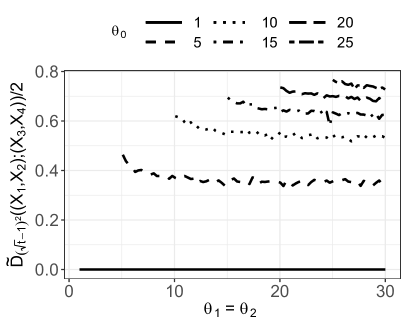
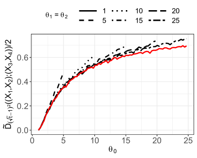
where is the generator of a Gumbel copula with parameter for satisfying and (sufficient nesting condition). We numerically approximate half the Hellinger distance using (17) with . Note that no estimation of the marginals is involved here. Figure 4 shows half the Hellinger distance as a function of for different values of , and as a function of for different values of .
Figure 4: Half Hellinger distance of copula (18) as a function of for different values of (left), and as a function of for different values of (right). The red line in the right plot shows half the Hellinger distance of a bivariate Gumbel copula with parameter .
Note that if , we have such that
meaning that and are independent.
In general, we observe that the strength of dependence between and is predominantly determined by the parameter . Nested Archimedean copulas allow us to on the one hand control the dependence within each random vector (by parameters and here) and on the other hand control what remains to be specified between the random vectors (parameter here). Notice that if and (i.e. and both tend to have a comonotonicity copula), the half Hellinger distance tends to the half Hellinger distance of a bivariate Gumbel copula with parameter (red line in the right plot).
Coming back to Remark 5, suppose we would compute the Hellinger distance of this bivariate Gumbel copula with parameter , say , using the non-simplified empirical version (15) (but now with known and a true sample from with fixed ) instead of , i.e. using
(19)
where for is a sample drawn from . Then, the pitfall is that
for since
for a fixed . The above can be seen from the fact that for the Gumbel generator , it holds that as . Hence, the law of large numbers still holds, but the convergence will be slower due to infinite variance, see also Section 6.2.
6. Simulation experiments
In this section, we perform some simulations that ought to complement the theoretical results that we obtained. First, we focus on Theorem 1 and investigate how well the asymptotic normal distribution approximates the finite-sample distribution of the plug-in estimator for the mutual information and Hellinger distance in case of a Gaussian copula model. Second, we numerically assess how well the estimator (15) performs in the setting of Example 6, and compare the numerical quality of given in (19) with the numerical quality of given in (17) within a bivariate Gumbel copula model.
6.1. Asymptotic normality under Gaussian copula model
Recall the asymptotic normality result of Theorem 1 for the estimator , with the matrix of sample normal scores rank correlation coefficients (8) and given in (5) and (6) for and respectively. We first turn our attention to Example 4 once more. In Figure 3, we depicted the asymptotic standard deviation
and . If we generate samples from e.g. a four dimensional multivariate Gaussian distribution with mean zero and covariance matrix as in Example 4, we obtain estimates of , say . An empirical Monte Carlo version of , with SD being the standard deviation, is then given by
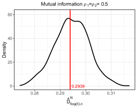
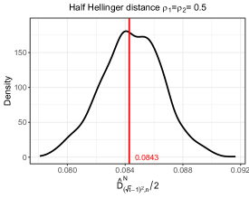
which we can compute for different values of and , see Figure 5 for some plots in case and . Comparing with Figure 3 of Example 4, this empirically verifies the formula for the asymptotic variance in Theorem 1 in this particular setting. Kernel density estimates for the density of when are included as well.
Figure 5: Empirical standard deviation (sample size ) and in the setting of Example 4, and kernel density estimates for and when and . The red vertical lines indicate the true value of the dependence coefficient.
Let now be the plug-in estimator of the asymptotic standard deviation obtained by using instead of the true . Based on a sample for from a certain multivariate distribution having a Gaussian copula, we are able to compute one realization of the actual sampling distribution of the studentized estimator
,
and several replications will give an idea about the entire distribution, which should, according to Theorem 1 approximately be a standard normal one for larger values of . We consider four settings which we can generate samples from:
•
Setting 1: , with standard normal marginals and a Gaussian copula having an autoregressive AR(1) correlation matrix with .
•
Setting 2: as Setting 1, but now with marginals
a distribution with degrees of freedom for
an exponential distribution with mean for
a beta distribution with parameters and for
an -distribution with degrees of freedom and for .
•
Setting 3: similar to Setting 1, but with .
•
Setting 4: , with standard normal marginals and a Gaussian copula having an equicorrelated correlation matrix with .
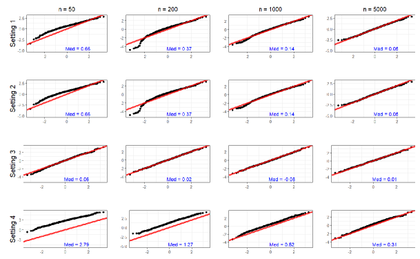
Mutual information
Figure 6: Normal Q-Q plots for Monte Carlo runs of the studentized plug-in estimator for the mutual information under four different settings with sample sizes . The median (“Med”) of the studentized estimates is indicated in blue.
Each time, we draw samples of sizes and make normal Q-Q plots to assess the goodness-of-fit with a standard normal distribution. See Figure 6 for the results of the mutual information, and Figure 7 for the half Hellinger distance.
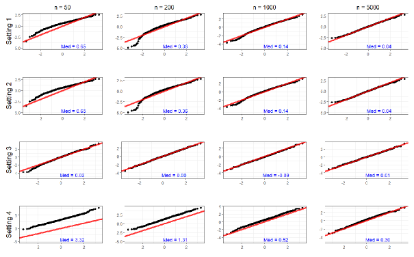
Half Hellinger distance
Figure 7: Normal Q-Q plots for Monte Carlo runs of the studentized plug-in estimator for the half Hellinger distance under four different settings with sample sizes . The median (“Med”) of the studentized estimates is indicated in blue.
In each setting, we have a qualitative normal approximation for larger sample sizes. Sampling from a multivariate normal distribution or from a multivariate normal copula with various marginals does not give a significant difference (Setting 1 versus Setting 2). For rather small correlations (Setting 1 and Setting 2), we observe a more pronounced lack-of-fit than for higher correlations (Setting 3). Increasing the total dimension to (Setting 4) results in a large positive bias for small sample size, which is no shock since empirical covariance matrices tend to be more biased when the number of parameters to estimate increases.
6.2. Nested Archimedean copula model
In the context of a general parametric copula family, the estimator (15) relies on an estimator for the copula parameter on the one hand, and on a numerical integral approximation on the other hand. In Example 6, we mathematically illustrated that, in a bivariate Gumbel copula with parameter , the estimator is doomed to have a slower convergence than the estimator relying on a simplified integral approximation as in (17).
Via a small simulation, we now compare the performance of these two estimators when and , based on samples drawn from this bivariate Gumbel copula. We consider and compare in Table 2 the sample bias, variance and mean squared error of and .
The estimator is based on maximizing the pseudo likelihood with non-parametric marginals, i.e. , using a starting value of . The true value of the dependence coefficient equals , and was computed, not by doing an empirical mean approximation of the two dimensional integral, but using numerical integration. As expected, the performance of is poor due to a large variance that needs very large values of to go down.
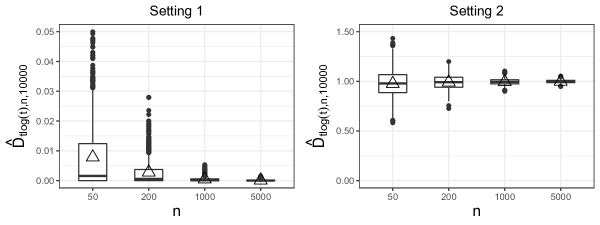
Next, we investigate how well the estimator performs in terms of increasing for the half Hellinger distance between and having the four dimensional copula given in (18) in Example 6. The estimator for the mutual information is also considered. We look at two settings:
•
Setting 1: , such that , since and are independent.
•
Setting 2: , such that and , computed via the true and samples to numerically approximate the integral.
bias
var
mse
bias
var
mse
Table 2: Sample bias, variance and mean squared error of two estimators for the half Hellinger distance in a bivariate Gumbel copula with parameter , based on replications, a sample size , and . The true value equals .
We take , with as starting value for for maximizing the likelihood. The starting values for and are taken as the maximizers of the individual pseudo likelihoods (also with non-parametric marginals) corresponding to the marginal samples of and respectively, with both starting values equal to . In each setting, we take Monte Carlo runs and sample sizes and fix for every .
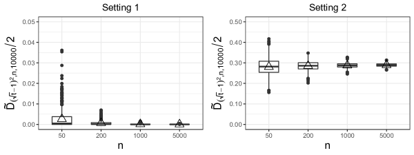
Figure 8: Boxplots of estimated dependence coefficients for different sample sizes in different settings. The triangles indicate the mean values.
Mutual information
Half Hellinger distance
Setting 1
Setting 2
Setting 1
Setting 2
Table 3: Empirical Monte Carlo variances of estimated dependence coefficients for different sample sizes in different settings, based on replications.
Boxplots are shown in Figure 8. For each dependence coefficient and in each setting, the bias and variance tend to zero when the sample size increases. Table 3 shows empirical Monte Carlo variances of each estimator. They indicate that cases of stronger dependence (Setting 2) are harder to estimate than cases of weak dependence (Setting 1) where the asymptotic variance is smaller (as we have seen for some Gaussian examples too).
7. A financial application
Quantifying the strength of relationship between variables is fundamental in finance, e.g. in portfolio management. Individual constituents are often (positively) related to one another because of contingency on macro-economic factors, known as systematic risk. For instance, market downturns can have detrimental consequences on the portfolio as association between assets can significantly increase. This phenomenon is known as asymmetric dependence, see e.g. Alcock and Satchell (2018). Closely related is the concept of financial contagion, e.g. Gallegati (2012), Celik (2012), Wang and Hui (2017) and Akhtaruzzaman et al. (2021), among others, evidencing stronger linkages across markets in times of recession.
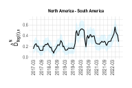
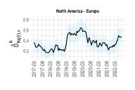
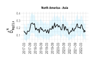
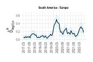
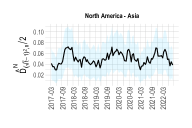
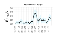
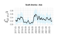
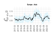
These markets can be considered within one and the same region, or can be spread over multiple different regions. We might for instance have a random vector describing equity indexes in North America and look at the intra-dependence, or investigate the inter-dependence with European indexes , neglecting the within region dependence. Here, we will use the -dependence measures between and , intending to illustrate cross-regional financial contagion during the COVID-19 pandemic.
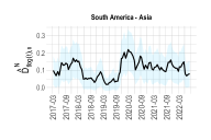
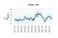
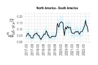
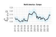
In particular, we analyse historical daily logarithmic returns of stock indexes from North-America (US S&P500, Canadian S&P/TSX Composite Index and Mexican IPC Index), South-America (Brazilian IBOVESPA and Argentina Merval Index), Europe (Euronext 100, German GDAXI, Spanish IBEX 35 and Norwegian OMX Index) and Asia (Japanese Nikkei 225, Chinese SSE Composite Index, Indian S&P BSE 500 and Hong Kong HSI Index), over a time span of Dec 07, 2016 to Dec 06, 2022. The data can freely be accessed and downloaded at https://finance.yahoo.com/. Notice that logarithmic returns are i.i.d. when assuming a random walk market. Each set of index returns in each continent is considered as a random vector , and inter-regional financial dependence is assessed as for .
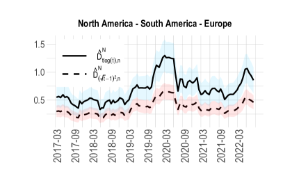
We first make use of the method discussed in Section 4, relying on the assumption of a Gaussian copula model. A primary impression of inter-regional financial contagion during the COVID-19 period is obtained by looking at the dependence over time. In total, we have non-missing log-returns in the given period that are common for each stock index. We divide this data into windows of size with slide step , i.e. and a final ’th window . Next, we compute for the returns in each window and assign this to the date corresponding to the left bound of that window. As such, we get an idea of how the dependence between groups of stock indexes across different continents evolved over time, keeping in mind that a certain date reflects the dependence calculated from the future days available in the dataset. Thanks to Theorem 1, we can also add approximated confidence bounds for each window, with the lower quantile of a standard normal distribution.
Figure 9: Estimated mutual information and half Hellinger distance between groups of equity indexes of different continents over time. Regions with confidence are shown in blue.
Figure 9 shows the results for the mutual information and half Hellinger distance with . In all cases, we observe a (for some more pronounced than others) hump during the first year of the pandemic, attracting our attention. In the first half of , the Corona pandemic gave rise to a stock market crash. Many indexes around the world were recovered by the end of . See Akhtaruzzaman et al. (2021) and references therein for more detailed information. We define the pre-crisis (period ) to be the period Dec 07, 2016 to Nov 29, 2019, the crisis period (period ) Dec 02, 2019 to Dec 30, 2020, and the post-crisis period (period ) as Jan 04, 2021 to Dec 06, 2022. For these respective periods, there are and observed log-returns available. Denote with for the Gaussian copula -dependence between and in period , with asymptotic standard deviation , and corresponding sample versions and . A test for financial contagion is
whose rejection provides statistical evidence for stronger linkages across markets during the crisis than before, and
whose rejection illustrates weaker inter-regional dependence after the crisis than during. Asymptotic approximate -values for these test are respectively given by
(20)
and
(21)
where and are the corresponding test values.
Financial contagion -values
Mutual information
Half Hellinger distance
NA - SA
NA - EU
NA - AS
SA - EU
SA - AS
EU - AS
Table 4: P-values (20) for test of increased linkages between inter-regional equity indexes from pre-crisis to crisis and (21) for test of decreased linkages from crisis to post-crisis, using the mutual information or half Hellinger distance as dependence measure (NA = North America, SA = South America, EU = Europe, AS = Asia).
For two continents neither of which is Asia, we have statistical evidence for inter-regional financial contagion at significance level . When Asia is included, we find larger -values, especially for .
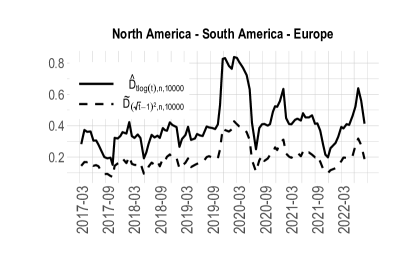
Figure 10: Estimated mutual information and Hellinger distance between equity indexes of North America, South America and Europa over time, using a Gaussian copula (left) and a nested Clayton copula (right).
Over the past year, vaccination campaigns in Asia have been losing efficiency, healthcare systems have been struggling, and putting an end to the Chinese Zero-COVID policy has led to a new flare-up.
We now look at the vector dependence between North America, South America and Europa simultaneously, not taking Asia into account. Figure 10 shows the estimated mutual information and Hellinger distance (we multiplied the half Hellinger distance with a factor in order to see the line more clearly) on the hand hand using the Gaussian copula approach (left) and on the other hand by fitting a nine dimensional nested Clayton copula (right) via the copula pseudo likelihood with non-parametrically estimated marginals using as starting value for the parameter of the root copula, and maximum likelihood estimates (also pseudo likelihood and non-parametric marginals) for the parameters of the child copulas, obtained with all three starting values equal to . We opt for the Clayton family, as possible lower tail dependence might be incorporated as well in this copula family. Using this latter estimation approach, i.e. or , where we took , the hump of increased dependence during the COVID-19 financial recession is even more expressed.
Finally, notice that returns can also be considered on a different periodicity, such as monthly returns. Longer horizons often allow to better capture the general trend as they are not affected so much by noise that might be present on a daily basis. For instance, as we are considering stock indexes from across the entire globe, trading hours depend on the geographic location and differences in opening and closing hours of the stock exchange might impact the dependence structure.
8. Discussion
In this paper, we started from the general objective of quantifying dependence between a finite, arbitrary amount of random vectors. We postulated desirable properties giving preference to a copula based perspective, and proved conformity for our proposed family of -dependence measures. A notion of perfect dependence is not among the axioms, but a characterization of it is possible for certain choices of , and was illustrated by means of examples.
Assuming a Gaussian copula model, an asymptotic normality result for the suggested plug-in estimator was established and could be interpreted further for specific -functions. Extensions to general parametric copula families were also obtained, focusing on maximum likelihood estimation and again a plug-in approach. Special attention went to nested Archimedean copulas, allowing for different parameters to control the intra- and inter-vector dependence. Simulations investigated finite-sample performances. In a real data analysis, the estimates indicate substantial levels of financial contagion during the COVID-19 recession.
Among the interests for further research are high-dimensional settings ( large), in which regularisation techniques are obliging. Also, semi- or non-parametric modelling of the copula can offer more flexible dependence capturing, and as such dig deeper than associations restricted to correlations (as in Gaussian copulas) and tail dependence (as in Archimedean copulas). These issues will be studied by the authors in future research.
Acknowledgement. The authors gratefully acknowledge support from the Research Fund KU Leuven [C16/20/002 project].
References
Akhtaruzzaman et al. (2021)
Akhtaruzzaman, M., Boubaker, S., and Sensoy, A.
Financial contagion during COVID–19 crisis.
Finance Res. Lett., 38:101604, 2021.
Alcock and Satchell (2018)
Alcock, J. and Satchell, S.
Asymmetric Dependence in Finance: Diversification, Correlation
and Portfolio Management in Market Downturns.
John Wiley & Sons, Chichester, England, 2018.
Celik (2012)
Celik, S.
The more contagion effect on emerging markets: The evidence of
DCC-GARCH model.
Econ. Model., 29(5):1946–1959, 2012.
Cover and Thomas (2006)
Cover, T. M. and Thomas, J. A.
Elements of Information Theory.
John Wiley & Sons, Hoboken, New Jersey, 2006.
De Keyser and Gijbels (2023)
De Keyser, S. and Gijbels, I.
Copula-based divergence measures for dependence between random
vectors.
In García-Escudero, L. A., Gordaliza, A., Mayo, A., Gomez, M.
A. L., Gil, M. A., Grzegorzewski, P., and Hryniewicz, O., editors,
Advances in Intelligent Systems and Computing, Vol. 1433, Building
Bridges between Soft and Statistical Methodologies for Data Science, pages
104–111. Springer, 2023.
Embrechts et al. (2002)
Embrechts, P., McNeil, A. J., and Straumann, D.
Correlation and dependence in risk management: properties and
pitfalls.
In Dempster, M., editor, Risk Management: Value at Risk and
Beyond, pages 176–223. Cambridge University Press, 2002.
Gallegati (2012)
Gallegati, M.
A wavelet-based approach to test for financial market contagion.
Stat. Data. Anal., 56(11):3491–3497,
2012.
Geenens and Lafaye de Micheaux (2022)
Geenens, G. and Lafaye de Micheaux, P.
The Hellinger correlation.
J. Am. Stat. Assoc., 117(538):639–653,
2022.
Geißer et al. (2010)
Geißer, S., Ruppert, M., and Schmid, F.
A multivariate version of Hoeffding’s Phi-Square.
J. Multivar. Anal., 101(10):2571–2586,
2010.
Genest et al. (1995)
Genest, C., Ghoudi, K., and Rivest, L.-P.
A semiparametric estimation procedure of dependence parameters in
multivariate families of distributions.
Biometrika, 82(3):543–552, 1995.
Gijbels et al. (2021)
Gijbels, I., Kika, V., and Omelka, M.
On the specification of multivariate association measures and their
behaviour with increasing dimension.
J. Multivar. Anal., 182:104704, 2021.
Grothe et al. (2014)
Grothe, O., Schnieders, J., and Segers, J.
Measuring association and dependence between random vectors.
J. Multivar. Anal., 123:96–110, 2014.
Hájek and Šidák (1967)
Hájek, J. and Šidák, Z.
Theory of Rank Tests.
Academia, Prague, 1967.
Hofert and Pham (2013)
Hofert, M. and Pham, D.
Densities of nested Archimedean copulas.
J. Multivar. Anal., 118:37–52, 2013.
Hotelling (1936)
Hotelling, H.
Relations between two sets of variates.
Biometrika, 28(3/4):321–377, 1936.
Joe (1989)
Joe, H.
Estimation of entropy and other functionals of a multivariate
density.
Ann. Inst. Statist. Math., 41(4):683–697,
1989.
Joe (1997)
Joe, H.
Multivariate Models and Dependence Concepts.
Chapman & Hall, London, New York, 1997.
Klaassen and Wellner (1997)
Klaassen, C. A. J. and Wellner, J. A.
Efficient estimation in the bivariate normal copula model: normal
margins are least favourable.
Bernoulli, 3(1):55–77, 1997.
Lancaster (1963)
Lancaster, H. O.
Correlation and complete dependence of random variables.
Ann. Math. Stat., 34(4):1315–1321, 1963.
Lehmann (1983)
Lehmann, E. L.
Theory of Point Estimation.
Springer-Verlag, New York, 1983.
Liese and Vajda (2006)
Liese, F. and Vajda, I.
On divergences and informations in statistics and information theory.
IEEE Trans. Inf. Theory, 52(10):4394–4412, 2006.
Majerek et al. (2005)
Majerek, D., Nowak, W., and Ziba, W.
Conditional strong law of large number.
Int. J. Pure. Appl. Math., 20(2):143–156,
2005.
McNeil et al. (2005)
McNeil, A. J., Frey, R., and Embrechts, P.
Quantitative Risk Management: Concepts, Techniques and Tools.
Princeton University Press, New Jersey, 2005.
Mordant and Segers (2022)
Mordant, G. and Segers, J.
Measuring dependence between random vectors via optimal transport.
J. Multivar. Anal., 189:104912, 2022.
Nelsen (1996)
Nelsen, R. B.
Nonparametric measures of multivariate association.
In Ruschendorf, L., Schweizer, B., and Taylor, M. D., editors,
Lecture Notes - Monograph Series Vol. 28, Distributions with Fixed
Marginals and Related Topics, pages 223–232. Institute of Mathematical
Statistics, 1996.
Nelsen (2006)
Nelsen, R. B.
An Introduction to Copulas.
Springer Science and Business Media, New York, 2006.
Okhrin and Ristig (2014)
Okhrin, O. and Ristig, A.
Hierarchical Archimedean copulae: The hac package.
J. Stat. Softw., 58(4):1–20, 2014.
Omelka et al. (2009)
Omelka, M., Gijbels, I., and Veraverbeke, N.
Improved kernel estimation of copulas: weak convergence and
goodness-of-fit testing.
Ann. Stat., 37(5B):3023–3058, 2009.
Österreicher and Vajda (2003)
Österreicher, F. and Vajda, I.
A new class of metric divergences on probability spaces and its
applicability in statistics.
Ann. Inst. Statist. Math., 55(3):639–653,
2003.
Rényi (1959)
Rényi, A.
On measures of dependence.
Math. Acad. Sci. Hungar., 10:441–451, 1959.
Schmid and Schmidt (2007)
Schmid, F. and Schmidt, R.
Multivariate extensions of Spearman’s rho and related statistics.
Stat. Probab. Lett., 77(4):407–416, 2007.
Schweizer and Wolff (1981)
Schweizer, B. and Wolff, E. F.
On nonparametric measures of dependence for random variables.
Ann. Stat., 9(4):879–885, 1981.
Sklar (1959)
Sklar, A.
Fonctions de repartition à n dimensions et leurs marges.
Publications de l’Institut Statistique de l’Université
de Paris, 8:229–231, 1959.
Wang and Hui (2017)
Wang, X. and Hui, X.
Mutual information based analysis for the distribution of financial
contagion in stock markets.
Discrete Dyn. Nat. Soc., 2017:3218042, 2017.
Wolff (1980)
Wolff, E. F.
-dimensional measures of dependence.
Stochastica, 4(3):175–188, 1980.
Appendix
Proof of Theorem 1
We first consider the specific cases and . Recall that for these cases, expression (4) reduces to (5) and (6), which are simpler expressions. Later in the proof, we look at the expression for for general .
Case
We start by showing the Fréchet differentiability of the map
From Corollary 4.5 in Mordant and Segers (2022), we have that the Fréchet derivative of at in the direction of a certain equals
with the diagonal matrix containing the diagonal of . Let now be such that as . Already note that will be in for small enough since . Consider now the function
Then, we see that and , where
with the diagonal block of . Jacobi’s formula in matrix calculus tells us that the Fréchet derivative of in the direction of is given by . Hence, the Fréchet derivative of the map
in the direction of equals
Furthermore, the Jacobian of is given by
such that the Fréchet derivative of (being nothing more than a total derivative) at in the direction of is equal to
Applying the chain rule, we have shown that the Fréchet derivative of at evaluated in equals
where the last equality follows from the exact same arguments as in Corollary 4.5 of Mordant and Segers (2022). Notice that this Fréchet derivative is linear, as it should be.
Case
We continue by showing the Fréchet differentiability of . Therefore, note that
By the chain rule, the Fréchet derivative of at in the direction of equals
From basic matrix calculus, the derivative of at evaluated in is
Obviously has the identity as derivative, and the product rule gives
as Fréchet derivative of . The derivative of at in the direction of , is the derivative of at in the direction of , i.e.
From this, it is easily seen that
is the derivative of , and, by using the product rule again,
is the Fréchet derivative of at evaluated in . Notice that the above derivative is not yet specifically of the from for a certain matrix . However, since all linear maps are of that form, and Fréchet derivatives are linear maps, we should be able to find such . Let
be the projection matrix onto the coordinates, satisfying , and
Observe that
using the cyclic trace property and the fact that
Knowing this, it is quickly seen that the Fréchet derivative of at in the direction of equals
General case
We now look at the Fréchet derivative of the integrand of in (4) for general . The derivative of in the direction of equals
By the chain rule, the derivative of evaluated at is
The derivative of in the direction of equals
Next, since the Jacobian of the function is
it is quickly seen that the Fréchet derivative of the factor in the integrand of (4) in front of in the direction of equals
Regarding the term within the -function, note that the derivative of evaluated in equals
such that, using a similar reasoning as before
is the Fréchet derivative of the term inside the -function in the direction of . Denote now for the density function of a distribution, and similarly . The product and chain rule tell us that the Fréchet derivative of the integrand of in the direction of is given by
Hence,
First of all, by definition
Furthermore, since a quadratic form is just a number, we also have that
(A1)
where we used the linearity and cyclic property of the trace operator, and a similar reasoning with the projection matrices as in the case . The other terms can be handled in a similar way, resulting in
Applying the delta method
Next, we consider the estimator . Theorem 3.1 in Klaassen and Wellner (1997) tells us that
as , where , with for , for is a sample from the distribution. The same expansion holds when is the empirical correlation matrix of , see e.g. Lemma 4.17 in Mordant and Segers (2022). Hence
as , i.e. making use of the empirical correlation matrix based on a true Gaussian sample or based on a pseudo Gaussian sample, results in the same asymptotic expansion. Suppose further that is the eigendecomposition of . Then for and a sample from . From Lemma 4.16 of Mordant and Segers (2022), we have
as , where is a random symmetric matrix with if and if independently (and similarly for ). Moreover, for , it holds that
We find
as .
Applying the delta method (and using that ), we obtain
as . The latter asymptotic expression is centered Gaussian with asymptotic variance
using the trace cyclical property and finishing the proof. ∎
Proof of Theorem 2
Note that because of the condition on , both estimators and have the same asymptotic normality result. The fact that is asymptotically normal, follows from the delta method. If furthermore we can interchange differentiation and integration, the Fréchet derivative (total derivative) of in the direction of is given by
Hence, an asymptotic normality result for ,
gives rise to an asymptotic normality result for , and thus for ,