Spherical Wavefronts Improve MU-MIMO Spectral Efficiency When Using Electrically Large Arrays

Abstract

Modern multiple-input multiple-output (MIMO) communication systems are almost exclusively designed under the assumption of locally plane wavefronts over antenna arrays. This is known as the far-field approximation and is soundly justified at sub-6-GHz frequencies at most relevant transmission ranges. However, when higher frequencies and shorter transmission ranges are used, the wave curvature over the array is no longer negligible, and arrays operate in the so-called radiative near-field region. This letter aims to show that the classical far-field approximation may significantly underestimate the achievable spectral efficiency of multi-user MIMO communications operating in the 30-GHz bands and above, even at ranges beyond the Fraunhofer distance. For planar arrays with typical sizes, we show that computing combining schemes based on the far-field model significantly reduces the channel gain and spatial multiplexing capability. When the radiative near-field model is used, interference rejection schemes, such as the optimal minimum mean-square-error combiner, appear to be very promising, when combined with electrically large arrays, to meet the stringent requirements of next-generation networks.

Sect. I Introduction and motivation

The increasing demand for ubiquitous, reliable, fast, and scalable wireless services is pushing today’s radio technology toward its ultimate limits. In this context, it is natural to continue searching for more bandwidth, which in turn pushes the operation towards higher frequencies [1]. 5G is designed to operate in bands up to $71$ GHz [2]. THz communications in the band from 0.1 to 10 THz is considered as a highly promising technology for 6G and beyond [1]. The use of high frequencies translates into higher path losses per antenna, which can be compensated for by antenna arrays. This combination undermines a fundamental assumption of multiple antenna communications: the wavefronts of radiated waves are locally planar over antenna arrays [3].

When an antenna radiates a wireless signal in free space, the wavefront of the electromagnetic waves has a different shape depending on the observation distance. Traditionally, two regions have been distinguished [4]: the Fresnel and the far-field regions. Wireless communications have almost exclusively operated in the antenna (array) far field, which is conventionally characterized by propagation distances beyond the Fraunhofer distance. When arrays between $10$ cm and $1$ m are utilized, the typical communication ranges up to $100$ m are almost entirely in the Fresnel region when using a carrier frequency in the range $30$–$300\,\mathrm{GHz}$ [5]. Thus, the plane wave approximation does not hold anymore, and spherical wavefront propagation must be considered instead [5]. This offers the opportunity for spatial-multiplexing in low-rank single-user MIMO systems [6, 7] and for high-accuracy estimation of source position [8]. However, this line of research constitutes a minor fraction of the vast literature that relies on the plane-wave approximation.

\begin{overpic}[width=433.62pt]{figures/fig1} \put(45.0,50.0){\footnotesize{$L_{\mathsf{H}}$}} \put(81.0,25.0){{\footnotesize{$L_{\mathsf{V}}$}}} \put(66.0,6.5){\footnotesize{$d_{\mathsf{H}}$}} \put(71.5,6.0){\footnotesize{$\sqrt{A}$}} \put(15.0,33.5){\rotatebox{90.0}{\footnotesize{$d_{\mathsf{V}}$}}} \put(15.0,41.0){\rotatebox{90.0}{\footnotesize{$\sqrt{A}$}}} \put(31.0,7.0){\footnotesize{$\mathbf{s}_{k}$}} \put(25.0,2.0){\footnotesize{$\varphi_{k}$}} \put(39.0,5.0){\footnotesize{$\theta_{k}$}} \put(13.0,12.0){\footnotesize{$\mathbf{r}_{1}$}} \put(82.0,49.0){\footnotesize{$\mathbf{r}_{N}$}} \put(93.0,30.0){\footnotesize{$X$}} \put(45.0,54.0){\footnotesize{$Y$}} \put(19.0,5.0){\footnotesize{$Z$}} \end{overpic}

Figure 1: Diagram of the 2D planar array located in the $XY$-plane.

Our objective is to show that, in the bands above $6$ GHz, the classical far-field approximation may profoundly underestimate the achievable performance of multi-user MIMO communication systems equipped with planar arrays of practical size, i.e., in the order of half-a-meter. The underestimation is already large in the mmWave band around $30\,\mathrm{GHz}$ bands, and is further exacerbated when higher frequencies are considered. Our numerical analysis also shows that, when the radiative near-field channel model is used, minimum mean-square-error (MMSE) combining vastly outperforms maximum ratio (MR), thanks to the sub-wavelength spatial resolution that largely increases its interference suppression capabilities. Particularly, MMSE combining enables serving very many user equipments; in the order of $1500$ UEs/km² per channel use (in line with 5G requirements [9]), while ensuring fairness across them (and thus significantly increasing the performance at the cell edge). This makes the combination of MMSE combining and electrically large arrays a promising candidate to meet the stringent capacity requirements of next-generation networks.

Sect. II System and signal model

We consider a planar array centered around the origin of the $XY$-plane, as shown in Figure 1. The array consists of $N_{\mathsf{V}}$ horizontal rows and $N_{\mathsf{H}}$ antennas per row, for a total of $N=N_{\mathsf{H}}N_{\mathsf{V}}$ antennas. Each antenna has an area $A$ and the spacing is $d_{\mathsf{H}}$ and $d_{\mathsf{V}}$ along the horizontal and vertical directions, respectively. Thus, the horizontal and vertical lengths of the array are $L_{\mathsf{H}}=N_{\mathsf{H}}\sqrt{A}+\left(N_{\mathsf{H}}-1\right)d_{\mathsf{H}}$ and $L_{\mathsf{V}}=N_{\mathsf{V}}\sqrt{A}+\left(N_{\mathsf{V}}-1\right)d_{\mathsf{V}}$, respectively. The antennas are numbered from left to right and from the bottom row to the top row so that antenna $n$ is located at $\mathbf{r}_{n}=\left[x_{n},y_{n},0\right]^{\mathsf{T}}$, where $x_{n}=\Delta_{\mathsf{H}}\left(-\frac{N_{\mathsf{H}}-1}{2}+\textrm{mod}\left(n-1,N_{\mathsf{H}}\right)\right)$ and $y_{n}=\Delta_{\mathsf{V}}\left(-\frac{N_{\mathsf{V}}-1}{2}+\left\lfloor{(n-1)}/{N_{\mathsf{H}}}\right\rfloor\right)$ with $\Delta_{\mathsf{H}}=\sqrt{A}+d_{\mathsf{H}}$ and $\Delta_{\mathsf{V}}=\sqrt{A}+d_{\mathsf{V}}$. We assume that $K$ single-antenna UEs communicate with the planar array depicted in Figure 1 and transmit signals with polarization in the $Y$ direction when traveling in the $Z$ direction [10]. LoS propagation is considered, as it becomes predominant when considering high frequencies (and hence shrinking the transmission range) [5]. We denote by $\mathbf{s}_{k}=\left[x_{k},y_{k},z_{k}\right]^{\mathsf{T}}$ the arbitrary location for source $k$ so that the signal impinges on the planar array with azimuth and elevation angles given by $\varphi_{k}=\tan^{-1}({x_{k}}/{z_{k}})$ and $\theta_{k}=\tan^{-1}({y_{k}}/{\sqrt{x_{k}^{2}+z_{k}^{2}}})$, respectively.

We let $\mathbf{h}_{k}=\left[h_{k1},\dots,h_{kN}\right]^{\mathsf{T}}\in\mathbb{C}^{N}$ denote the channel of UE $k$. In particular, $h_{kn}=\left|h_{kn}\right|e^{-\mathsf{j}\phi_{kn}}$ is the channel from source $k$ to receive antenna $n$, with $\left|h_{kn}\right|^{2}$ being the channel gain and $\phi_{kn}\in\left[0,2\pi\right)$ denoting the phase shift. In the remainder, perfect channel state information is assumed, since the channels $\left\{\mathbf{h}_{k}\right\}_{k=1}^{K}$ can be estimated arbitrarily well from pilot signals, thanks to the line-of-sight (LoS) propagation.

II-A Channel model

To model $\mathbf{h}_{k}$, we extend the prior work [10], which only considers the case $d_{\mathsf{H}}=d_{\mathsf{V}}=\sqrt{A}$. The extension to the case $d_{\mathsf{H}}\neq d_{\mathsf{V}}$ with $d_{\mathsf{H}},d_{\mathsf{V}}\geq\sqrt{A}$ is as follows.

$$\zeta_{kn}=\frac{1}{12\pi}\sum_{i=0}^{1}{\sum_{j=0}^{1}{\frac{g_{i}\left(x_{kn}\right)g_{j}\left(y_{kn}\right)\left|z_{k}\right|}{\left(g_{j}^{2}\left(y_{kn}\right)+z_{k}^{2}\right)\sqrt{g_{i}^{2}\left(x_{kn}\right)+g_{j}^{2}\left(y_{kn}\right)+z_{k}^{2}}}}}+ \frac{1}{6\pi}\sum_{i=0}^{1}{\sum_{j=0}^{1}{\tan^{-1}\left(\frac{g_{i}\left(x_{kn}\right)g_{j}\left(y_{kn}\right)}{\left|z_{k}\right|\sqrt{g_{i}^{2}\left(x_{kn}\right)+g_{j}^{2}\left(y_{kn}\right)+z_{k}^{2}}}\right)}}$$ (1)

 

Corollary 1.

Consider a lossless isotropic antenna located at $\mathbf{s}_{k}$ that transmits a signal that has polarization in the $Y$ direction when traveling in the $Z$ direction. The free-space channel gain $\zeta_{kn}$ at the $n$th receive antenna, located at $\mathbf{r}_{n}$ is given by (1), shown at the top of the page, where

$$g_{i}\left(\alpha\right)\triangleq\sqrt{A}/2+\left(-1\right)^{i}\alpha$$ (2)

while $x_{kn}=x_{k}-x_{n}$ and $y_{kn}=y_{k}-y_{n}$. $\blacksquare$

From Corollary 1, the following model is obtained.

Corollary 2 (Exact model).

The channel entry $h_{kn}=\left|h_{kn}\right|e^{-\mathsf{j}\phi_{kn}}$ is obtained as

$$\left|h_{kn}\right| =\sqrt{\zeta_{k,n}}$$ (3)

$$\phi_{kn} =2\pi\,\textrm{mod}\left(\frac{\left\|\mathbf{d}_{kn}\right\|}{\lambda},1\right)$$ (4)

where $\zeta_{kn}$ is defined in (1) and $\mathbf{d}_{kn}={\mathbf{s}_{k}}-{\mathbf{r}_{n}}$. $\blacksquare$

The above model provides a general expression for $h_{kn}$ that allows to quantify its channel gain in the so-called radiative near-field of the array [11, 10]. Since it captures the fundamental properties of wave propagation, we call it the exact model. Notice that it is substantially different from the classical far-field model, e.g., [3], that assumes locally planar wavefronts over arrays and is valid for distances beyond the Fraunhofer distance $d_{F}=2\left(L_{\mathsf{H}}^{2}+L_{\mathsf{V}}^{2}\right)/\lambda$ [12, Eq. (3)].

Figure 2: Difference in the amplitude (left axis) and phase (right axis) between the exact model and the far-field approximation.

Corollary 3 (Far-field approximation).

If UE $k$ is in the far-field region of the array, i.e., $d_{k}\cos\varphi_{k}\gg\max\left(L_{\mathsf{H}},L_{\mathsf{V}}\right)$, then $h_{kn}\approx h_{kn}^{\rm FF}$ with $h_{kn}^{\rm FF}=\left|h_{kn}^{\rm FF}\right|e^{-\mathsf{j}\phi_{kn}}$ being modeled as

$$\left|h_{kn}^{\rm FF}\right|=\sqrt{\frac{A\cos\varphi_{k}}{4\pi d_{k}^{2}}}$$ (5)

$$\phi_{kn}^{\rm FF}=\mathbf{k}^{\mathsf{T}}\left(\varphi_{k},\theta_{k}\right)\mathbf{r}_{n}$$ (6)

where $\mathbf{k}\left(\varphi_{k},\theta_{k}\right)=\frac{2\pi}{\lambda}\left[\cos\theta_{k}\sin\varphi_{k},\sin\theta_{k},\right.$ $\left.\cos\theta_{k}\cos\varphi_{k}\right]^{\mathsf{T}}$ is the wave vector, e.g., [13]. $\blacksquare$

We notice that the propagation channel in MIMO systems has been almost exclusively modeled as in Corollary 3. For modern arrays of cellular networks of size $1\times 0.5\,\mathrm{m}^{2}$, this is a justified assumption when sub$-6$ GHz bands are used. In this case, $d_{F}\leq 50\,\mathrm{m}$ and, thus, most receivers are in the far-field of the transmitter. The situation changes substantially in the frequency range $30$-$300\,\mathrm{GHz}$, in which $d_{F}\geq 250\,\mathrm{m}$, and typical operating distances are entirely below it. This implies that the far-field approximation cannot be used, and the exact propagation model derived in Corollary 1 must be considered instead. As is known, the radiative near-field can create both noticeable amplitude variations and phase variations over the wavefront. To measure the impact of such variations, Figure 2 reports the results for $L_{\mathsf{H}}=0.5\,\mathrm{m}$, $L_{\mathsf{V}}=1.0\,\mathrm{m}$, $A=\left(\lambda/4\right)^{2}$, $d_{\mathsf{H}}=0.5\lambda$, and $d_{\mathsf{H}}=2\lambda$, considering a UE located at $30\,\mathrm{m}$ from the base station (BS), which is elevated by $10\,\mathrm{m}$. Amplitude variations are reported with dotted lines (using the left axis), whereas phase variations are represented by the solid lines (using the right axis). While the amplitude variations are negligible, the phase variations are significant, particularly when the carrier frequency increases.

Note that the model in Corollary 1 is also accurate in the far-field, thus there is no need to determine beforehand if the communication scenario is in the radiative near-field region or not. We conclude by noticing that the above discussion does not require the use of physically large arrays (cf. [15]), but holds true for commercially-sized arrays, e.g., in the order of half-a-meter wide and height. What matters is the size relative to the wavelength, the so-called electromagnetic size.

II-B System model

We consider the uplink. The received signal is modeled as $\mathbf{y}\in\mathbb{C}^{N}=\sum_{k=1}^{K}{\mathbf{h}_{k}s_{k}}+\mathbf{n}$, where $s_{k}\sim\mathcal{N}_{\mathbb{C}}\left(0,p_{k}\right)$ is the data from UE $k$ and $\mathbf{n}\in\mathbb{C}^{N}$ is the thermal noise with i.i.d. elements distributed as $\mathcal{N}_{\mathbb{C}}\left(0,\sigma^{2}\right)$. To decode $s_{k}$, $\mathbf{y}$ is processed with the combining vector $\mathbf{v}_{k}\in\mathbb{C}^{N}$. By treating the interference as noise, the spectral efficiency (SE) for UE $k$ is $\log_{2}\left(1+\gamma_{k}\right)$, where

$$\gamma_{k}=\frac{p_{k}\left|\mathbf{v}_{k}^{\mathsf{H}}\mathbf{h}_{k}\right|^{2}}{\sum_{i\neq k}{p_{i}\left|\mathbf{v}_{k}^{\mathsf{H}}\mathbf{h}_{i}\right|^{2}}+\sigma^{2}\left\|\mathbf{v}_{k}\right\|^{2}}$$ (7)

is the signal-to-interference-plus-noise ratio (SINR). We consider both MR and MMSE combining. MR has low computational complexity and maximizes the power of the desired signal, but neglects interference. MMSE has higher complexity but it maximizes the SINR in (7). Other suboptimal schemes, e.g. zero-forcing, are not considered for space limitation. In the first case, $\mathbf{v}_{k}^{\rm MR}=\mathbf{h}_{k}/\left\|\mathbf{h}_{k}\right\|$, while in the second case

$$\mathbf{v}_{k}^{\rm MMSE}=\left(\sum_{i=1}^{K}{{p_{i}\mathbf{h}_{i}\mathbf{h}_{i}^{\mathsf{H}}}}+{\sigma^{2}}\mathbf{I}_{N}\right)^{-1}\mathbf{h}_{k}$$ (8)

with $\mathbf{I}_{N}$ being the identity matrix of order $N$.

The vast majority of MIMO literature for high frequencies (e.g., in the mm-Wave frequency bands) rely on the far-field approximation in Corollary 3 and, instead of estimating $\mathbf{h}_{k}$ directly, estimate the three parameters $\{d_{k},\theta_{k},\varphi_{k}\}$. The latter are used to obtain estimates of $\{\mathbf{h}^{\rm FF}_{k};k=1,\ldots,K\}$ through (5) and (6), which are eventually used to compute the combiner. If the communication scenario is in the radiative near-field region, then the system operates inevitably in a mismatched mode, no matter how good $\{d_{k},\theta_{k},\varphi_{k}\}$ have been estimated. From the above discussion, it thus follows that the combining vectors $\left\{\mathbf{v}_{k}\right\}_{k=1}^{K}$ can in practice follow either the exact model defined in Corollary 2 or the far-field approximation defined in Corollary 3. The aim of this letter is to quantify the impact of such inaccurate channel modeling.

Sect. III The impact of a mismatched design

We assume that the BS is located at a height of $b=10\,\mathrm{m}$. We further assume the following parameters, in line with the form factor of current 5G arrays: $L_{\mathsf{H}}=0.5\,\mathrm{m}$, $L_{\mathsf{V}}=1.0\,\mathrm{m}$, $A=\left(\lambda/4\right)^{2}$, $d_{\mathsf{H}}=0.5\lambda$ and $d_{\mathsf{V}}=2\lambda$. The communication takes places over a bandwidth of $B=100\,\mathrm{MHz}$, with the total receiver noise power $\sigma^{2}=-87\,\mathrm{dBm}$. Each UE transmits with power $p_{k}=20\,\mathrm{dBm}$ $\forall k$. We assume a carrier frequency of $f_{0}=28\,\mathrm{GHz}$ such that $\lambda=10.71\,\mathrm{mm}$, $N_{\mathsf{H}}=62$, and $N_{\mathsf{V}}=42$, to focus on a 5G hot-spot scenario. When relevant, throughout the letter, we also consider higher carrier frequencies that cover future use cases and scenarios.

III-A Channel gain

We consider UE 1 and assume that it is located along the $Z$ axis with coordinates $\mathbf{s}_{1}=\left[0,-b,d\right]^{\mathsf{T}}$. In Figure 3, the dashed black line reports the normalized channel gain $\left|\mathbf{v}_{1}^{\mathsf{H}}\mathbf{h}_{1}\right|^{2}/\left\|\mathbf{v}_{1}\right\|^{2}$ achieved with the exact model, whereas the solid lines correspond to the channel gain measured with the combiners based on the far-field model. Particularly, the cyan and the blue lines refers to the cases $f_{0}=5\,\mathrm{GHz}$ and $f_{0}=28\,\mathrm{GHz}$, respectively, whereas the red and the green lines refer to $f_{0}=71\,\mathrm{GHz}$ and $f_{0}=300\,\mathrm{GHz}$, respectively. Markers correspond to the Fraunhofer distances, obtained as $d_{F}=2\left(L_{\mathsf{H}}^{2}+L_{\mathsf{V}}^{2}\right)/\lambda$ [12, Eq. (3)]. For $f_{0}=300\,\mathrm{GHz}$, $d_{F}=2.5\,\mathrm{km}$ falls outside the selected range.

We see that, thanks to the large values of $N$, the channel gain with the exact model depends very weakly on the carrier frequency (a difference of at most $0.3\,\mathrm{dB}$ between $5$ and $300$ GHz at the local maximum of the curve), and we thus only report one line, for clarity. The same channel gain is achieved with the mismatched model only for sub-$6\,\mathrm{GHz}$ frequencies, irrespective of the distance. This validates the accuracy of the far-field approximation for such frequency bands. On the contrary, if higher frequencies are considered, then large differences are observed for transmission ranges below the Fraunhofer distance. This is a direct consequence of the inaccuracy of the far-field approximation in the Fresnel region. The gap increases as $f_{0}$ increases. Interestingly, we observe that, for transmission ranges of practical interest (up to a hundred of meters), it is significant already for $f_{0}\geq 71\,$GHz. Finally, note that the normalized channel gain is not monotonically decreasing as the distance from the BS increases, but shows a local maximum. This is due to the specific choice of the BS height $b$: when the UE is too close to the BS, the smaller path loss is overwhelmed by the loss due to the array directivity at larger elevations. Thus, the local maximum increases as $b$ increases.

\begin{overpic}[width=476.98463pt]{figures/fig3} \put(74.5,27.5){\footnotesize{$d_{F}$}} \put(73.5,27.0){\vector(-2,-1){7.0}} \put(78.0,26.0){\vector(1,-3){3.5}} \put(72.5,28.0){\vector(-3,1){34.0}} \end{overpic}

Figure 3: Normalized channel gain $\left|\mathbf{v}_{1}^{\mathsf{H}}\mathbf{h}_{1}\right|^{2}/\left\|\mathbf{v}_{1}\right\|^{2}$ as a function of the distance of UE $1$ along $Z$ axis.

III-B Interference gain

We now analyze the normalized interference gain $\left|\mathbf{v}_{1}^{\mathsf{H}}\mathbf{h}_{2}\right|^{2}/\left\|\mathbf{v}_{1}\right\|^{2}$ with the exact and mismatched models. We assume UE $1$ is placed at a fixed position along the $Z$ axis $\mathbf{s}_{1}=\left[0,-10\,\mathrm{m},+20\,\mathrm{m}\right]^{\mathsf{T}}$, whereas the interfering UE $2$ is transmitting from different locations $\mathbf{s}_{2}=\left[x_{2},-10\,\mathrm{m},z_{2}\right]^{\mathsf{T}}$ over the $XZ$-plane (i.e., at the same height as UE $1$). We assume $f_{0}=28\,\mathrm{GHz}$ and consider both MR and MMSE. Note that, at $f_{0}=28\,\mathrm{GHz}$, $d_{F}\approxeq 233.3\,\mathrm{m}$, and hence both UEs are in the near-field region.

Figure 4 reports the normalized interference gain with the exact model. MMSE combining is used in Figure 44(a), whereas the MR is considered in Figure 44(b). Each figure contains a magnification around UE $1$’s location, in which the relative distance of UE $2$ from UE $1$ is measured in wavelengths (for a total span of around $1.07\times 1.07\,\mathrm{m}^{2}$). Figure 44(a) shows that the interference with MMSE is high only in a small region around UE $1$, whose semi-major axis (along both directions) is fractions of the wavelength. This means that MMSE can efficiently reject any interfering signal that comes from a location that is at least a few centimeters away. On the contrary, Figure 44(b) shows that MR experiences high interference from locations that are either along the $Z$ direction or along a semi-circle with radius equal to the distance of UE $1$.

\begin{overpic}[width=476.98463pt]{figures/fig4a} \put(56.0,34.0){\scriptsize{{\color[rgb]{1,1,1}\acs{UE} $1$'s position}}} \put(55.0,7.0){\framebox(0.0,0.0)[bl]{\includegraphics[scale={.16}]{figures/fig4a_zoom}}} \put(59.5,33.0){\color[rgb]{1,1,1}\vector(1,-2){8.0}} \put(55.7,33.0){\color[rgb]{1,1,1}\vector(-1,-1){6.0}} \end{overpic}

(a) MMSE combining.

\begin{overpic}[width=476.98463pt]{figures/fig4b} \put(56.0,34.0){\scriptsize{{\color[rgb]{1,1,1}\acs{UE} $1$'s position}}} \put(55.0,7.0){\framebox(0.0,0.0)[bl]{\includegraphics[scale={.16}]{figures/fig4b_zoom}}} \put(59.5,33.0){\color[rgb]{1,1,1}\vector(1,-2){8.0}} \put(55.7,33.0){\color[rgb]{1,1,1}\vector(-1,-1){6.0}} \end{overpic}

(b) MR combining.

Figure 4: Interference gain behavior using the exact model for a fixed UE as a function of different locations of an interfering UE.

\begin{overpic}[width=476.98463pt]{figures/fig5a} \put(56.0,34.0){\scriptsize{{\color[rgb]{1,1,1}\acs{UE} $1$'s position}}} \put(55.0,7.0){\framebox(0.0,0.0)[bl]{\includegraphics[scale={.16}]{figures/fig5a_zoom}}} \put(59.5,33.0){\color[rgb]{1,1,1}\vector(1,-2){8.0}} \put(55.7,33.0){\color[rgb]{1,1,1}\vector(-1,-1){6.0}} \end{overpic}

(a) MMSE combining.

\begin{overpic}[width=476.98463pt]{figures/fig5b} \put(56.0,34.0){\scriptsize{{\color[rgb]{1,1,1}\acs{UE} $1$'s position}}} \put(55.0,7.0){\framebox(0.0,0.0)[bl]{\includegraphics[scale={.16}]{figures/fig5b_zoom}}} \put(59.5,33.0){\color[rgb]{1,1,1}\vector(1,-2){8.0}} \put(55.7,33.0){\color[rgb]{1,1,1}\vector(-1,-1){6.0}} \end{overpic}

(b) MR combining.

Figure 5: Interference gain behavior using the mismatched model for a fixed UE as a function of different locations of an interfering UE.

Figure 5 plots the results obtained with the mismatched model. Unlike Figure 4, we now see that the interference gain with the two combining strategies exhibits a similar behaviour. The impact of the mismatched model is particularly evident with the MMSE combiner. In particular, we observe that the lower values of the interference gain are at least three orders of magnitude higher than those in Figure 4 (note that the same colorbar scale is used in all figures, including the magnifications). The conclusion is that MMSE can suppress interference much more efficiently when used with the exact model, whereas MR is greatly suboptimal in both cases.

III-C Spectral efficiency analysis

We now evaluate the SE of a single-cell network, assuming that $K$ UEs are randomly displaced in the sector $\left[-\pi/3,+\pi/3\right)$ with a minimum distance of $15\,\mathrm{m}$ from BS.

Figure 6 reports the cumulative distribution function (CDF) of the SE achieved by MMSE and MR when the carrier frequency is $f_{0}=5\,\mathrm{GHz}$, $28\,\mathrm{GHz}$, and $71\,\mathrm{GHz}$. The number of UEs is $K=100$, and the cell radius is $R=230\,\mathrm{m}$, which corresponds approximately to the Fraunhofer distance at $28\,\mathrm{GHz}$, and is in line with current 5G cell sizes. The dashed and solid refer to the results obtained with the exact and mismatched model, respectively. Let us focus on the results of Figure 66(a), obtained with the MMSE combiner. For all frequencies, the performance using the exact model to build the combiner is much better than the one obtained with the mismatched model. However, increasing the carrier frequency has a two-fold beneficial impact on the SE. On the one hand, the average SE increases as $f_{0}$ increases. On the other hand, the CDF with the exact model exhibits a steeper behavior, meaning that more fairness across the UE positions is guaranteed. The conclusion is that the use of the exact model dramatically improves the interference suppression capabilities of MMSE combining. This is not the case with MR combining. Indeed, Figure 66(b) shows that only marginal differences exist between exact and mismatched models, including the fairness properties.

A similar conclusion can be drawn in Figure 77(a), which collects the CDFs for the SE achieved by MMSE and MR combiners for a variable number of UEs ($K=50$, $100$, and $150$) when $f_{0}=28\,\mathrm{GHz}$ and $R=230\,\mathrm{m}$. We notice that the results are only marginally affected by the number of UEs when the exact model is used to build the combiner (dashed lines). This is not true for the combiners based on the mismatched model (solid lines) and/or based on MR combining (not reported here for the sake of brevity, as, similarly to Figure 66(b), both models provide very similar results when using MR combining). The same conclusion applies on the fairness performance, which is guaranteed by the usage of MMSE combining based on the exact model.

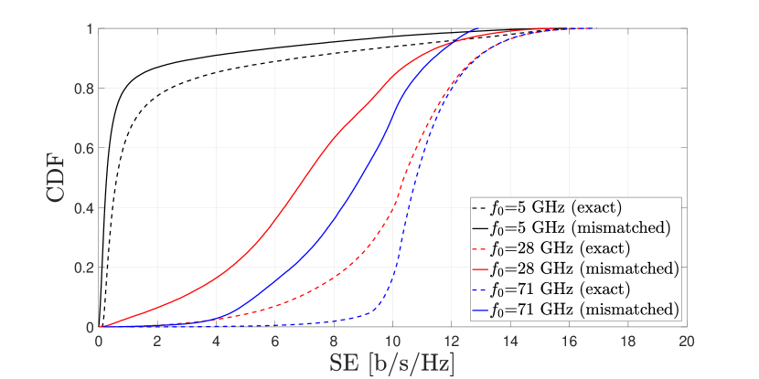
(a) MMSE combining.

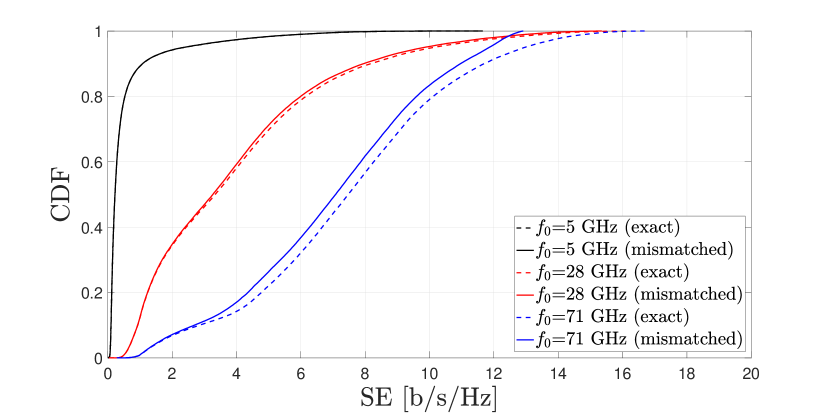
(b) MR combining.

Figure 6: CDF of the SE as a function of the carrier frequency when $K=100$ and $R=230$ m, corresponding to the Fraunhofer distance at $28\,\mathrm{GHz}$.

To further quantify the benefits brought by MMSE combining with the exact model, Figure 77(b) provides the average SE per UE as a function of $K$. The cell sector radius $R$ is $230\,\mathrm{m}$, and the carrier frequency is $f_{0}=28\,\mathrm{GHz}$. As can be seen, the gap between the exact and mismatched models is very significant. Moreover, the SE maintains nearly flat as $K$ increases up to $K=100$, which translates into a density of around $1500$ devices/km² per channel use, as requested in 5G [9]. Note that the excellent interference suppression capabilities let MMSE based on the exact model maintain the gap with other schemes when $K$ reaches very large values. The same trend is confirmed when measuring the average SE per UE as a function of $R$ (not reported for the sake of brevity): the performance gap using current 5G frequencies is very significant for $R\leq 50\,\mathrm{m}$, and even more significant when considering sub-THz frequencies and smaller cell sizes.

Sect. IV Conclusion

The main conclusion of this letter is that it is time for multi-user MIMO communication theorists to abandon the far-field approximation when considering carrier frequencies above $6$ GHz. We instead need to consider more complicated channel models that capture the radiative near-field characteristics, in particular concerning the spherical phase variations. This also affects beamforming codebooks. We showed that interference-aware combining schemes based on the radiative near-field model can effectively exploit the extra degrees-of-freedom offered by the propagation channel to deal with interference so as to enhance the scalability (in terms of number of UEs) and fairness of the system. This applies already to 5G multi-user MIMO communications above $6$ GHz (e.g., in the range of mmWave bands), and will be further exacerbated by beyond-5G communications, operating in the sub-THz spectrum.

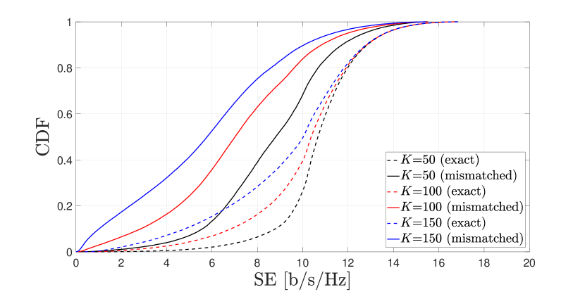
(a) CDF of the SE with MMSE combining for different values of $K$.

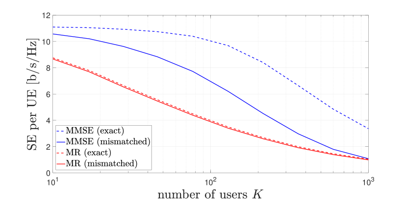
(b) SE per UE of both MMSE and MR as a function of $K$.

Figure 7: Impact of the number of active UEs on the SE performance.

References

- [1] T. S. Rappaport, Y. Xing, O. Kanhere, S. Ju, A. Madanayake, S. Mandal, A. Alkhateeb, and G. C. Trichopoulos, “Wireless communications and applications above 100 GHz: Opportunities and challenges for 6G and beyond,” IEEE Access, vol. 7, pp. 78 729–78 757, Jun. 2019.
- [2] 3rd Generation Partnership Project (3GPP), “Technical specification group radio access network; NR; Physical channels and modulation (Release 17),” Tech. Rep. 3GPP TS 38.211 V17.3.0, Sep. 2022.
- [3] R. W. Heath Jr. and A. Lozano, Foundations of MIMO Communication. Cambridge University Press, 2018.
- [4] K. T. Selvan and R. Janaswamy, “Fraunhofer and Fresnel distances: Unified derivation for aperture antennas,” IEEE Ant. Prop. Mag., vol. 59, no. 4, pp. 12–15, Aug. 2017.
- [5] H. Do, S. Cho, J. Park, H.-J. Song, N. Lee, and A. Lozano, “Terahertz line-of-sight MIMO communication: Theory and practical challenges,” IEEE Commun. Mag., vol. 59, no. 3, Mar. 2021.
- [6] F. Bøhagen, P. Orten, and G. E. Øien, “On spherical vs. plane wave modeling of line-of-sight MIMO channels,” IEEE Trans. Commun., vol. 57, no. 3, Mar. 2009.
- [7] E. Torkildson, U. Madhow, and M. Rodwell, “Indoor millimeter wave MIMO: Feasibility and performance,” IEEE Trans. Wireless Commun., vol. 10, no. 12, pp. 4150–4160, Dec. 2011.
- [8] B. Friedlander, “Localization of signals in the near-field of an antenna array,” IEEE Trans. Signal Process., vol. 67, no. 15, Aug. 2019.
- [9] Radiocommunication sector of International Telecommunication Union (ITU-R), “Minimum requirements related to technical performance for IMT-2020 radio interface(s),” Tech. Rep. ITU-R M.2410-0, Nov. 2017.
- [10] E. Björnson and L. Sanguinetti, “Power scaling laws and near-field behaviors of massive MIMO and intelligent reflecting surfaces,” IEEE Open J. Commun. Society, vol. 1, pp. 1306–1324, Sep. 2020.
- [11] D. Dardari, “Communicating with large intelligent surfaces: Fundamental limits and models,” IEEE J. Sel. Areas Commun., vol. 38, no. 11, pp. 2526–2537, Nov. 2020.
- [12] E. Björnson, Ö. T. Demir, and L. Sanguinetti, “A primer on near-field beamforming for arrays and reconfigurable intelligent surfaces,” in Proc. Asilomar, Pacific Grove, CA, USA, Nov. 2021.
- [13] E. Björnson, J. Hoydis, and L. Sanguinetti, “Massive MIMO networks: Spectral, energy, and hardware efficiency,” Foundations and Trends in Signal Processing, vol. 3-4, no. 11, 2017.
- [14] Ericsson. (2022) Massive MIMO solutions accelerate 5G mid-band. [Online]. Available: https://www.ericsson.com/en/ran/massive-mimo
- [15] H. Lu and Y. Zeng, “How does performance scale with antenna number for extremely large-scale MIMO?” in Proc. IEEE Int. Conf. Commun. (ICC), Montreal, Canada, Jun. 2021.