Systematic KMTNet Planetary Anomaly Search. VIII. Complete Sample of 2019 Subprime Field Planets

Abstract

We complete the publication of all microlensing planets (and “possible planets”) identified by the uniform approach of the KMT AnomalyFinder system in the 21 KMT subprime fields during the 2019 observing season, namely KMT-2019-BLG-0298, KMT-2019-BLG-1216, KMT-2019-BLG-2783, OGLE-2019-BLG-0249, and OGLE-2019-BLG-0679 (planets), as well as OGLE-2019-BLG-0344, and KMT-2019-BLG-0304 (possible planets). The five planets have mean log mass-ratio measurements of $(-2.6,-3.6,-2.5,-2.2,-2.3)$, median mass estimates of $(1.81,0.094,1.16,7.12,3.34)\,M_{\rm Jup}$, and median distance estimates of $(6.7,2.7,5.9,6.4,5.6)\,{\rm kpc}$, respectively. The main scientific interest of these planets is that they complete the AnomalyFinder sample for 2019, which has a total of 25 planets that are likely to enter the statistical sample. We find statistical consistency with the previously published 33 planets from the 2018 AnomalyFinder analysis according to an ensemble of five tests. Of the 58 planets from 2018-2019, 23 were newly discovered by AnomalyFinder. Within statistical precision, half of all the planets have caustic crossings while half do not (as predicted by Zhu et al. 2014), an equal number of detected planets result from major-image and minor-image light-curve perturbations, and an equal number come from KMT prime fields versus subprime fields.

1 Introduction

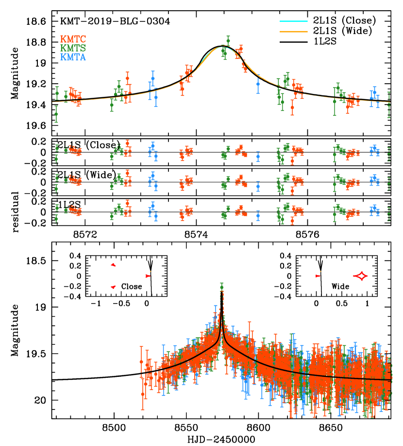
Figure 12: Data (color-coded by observatory) together with the predictions and residuals for the two planetary models of KMT-2019-BLG-0304 specified in Table 12, as well as the 1L2S model specified in Table 13. All three models can explain the data equally well. Hence, this event cannot be cataloged as “planetary”.

We present the analysis of all planetary events that were identified by the KMTNet AnomalyFinder algorithm (Zang et al., 2021, 2022) and occurred during the 2019 season within the 21 subprime KMTNet fields, covering $\sim 84\,{\rm deg}^{2}$ that lie in the periphery of the richest microlensing region of the Galactic bulge, and which are observed with cadences $\Gamma=0.2$–$1\,{\rm hr}^{-1}$. This work follows the publications of complete samples of the 2018 prime (Wang et al., 2022; Hwang et al., 2022; Gould et al., 2022), and subprime (Jung et al., 2022) AnomalyFinder events, the 2019 prime (Zang et al., 2021; Hwang et al., 2022; Zang et al., 2022) events, as well as a complete sample of all events from 2016-2019 with planet-host mass ratios $q<10^{-4}$ (Zang et al., 2023). The above references are (ignoring duplicates) Papers I, IV, II, III, V, VI, and VII, in the AnomalyFinder series. The locations and cadences of the KMTNet fields are shown in Figure 12 of Kim et al. (2018a). Our immediate goal, which we expect to achieve within a year, is to publish all AnomalyFinder planets from 2016-2019. Over the longer term, we plan to apply AnomalyFinder to all subsequent KMT seasons, beginning 2021.

For the 2019 subprime fields, the AnomalyFinder identified a total of 182 anomalous events (from an underlying sample of 1895 events), which were classified as “planet” (9), “planet/binary” (10), “binary/planet” (18), “binary” (136), and “finite source” (9). Among the 136 in the “binary” classification, 56 were judged by eye to be unambiguously non-planetary in nature. Among the 9 in the “planet” classification, 4 were previously published (including 2 AnomalyFinder discoveries), while one had been recognized but remained unpublished. Among the 10 in the “planet/binary” classification, 3 were either published planets (1) or had been recognized by eye (2), and among the 18 in the “binary/planet” classification, one was a previously published planet. Among the 136 classified as “binary”, 1 (a two-planet system) was published. Thus, in total, the AnomalyFinder recovered 9 planets that had been previously found by eye, including 6 that were published and 3 others that had not been published. The latter are KMT-2019-BLG-1216, OGLE-2019-BLG-0249, and OGLE-2019-BLG-0679.

Our overall goal is to present full analyses of all events with mass ratios $q<0.03$. To this end, we carry out systematic investigations of all of the AnomalyFinder candidates (other than the 56 classified by eye as unambiguously non-planetary) using end-of-season pipeline data. Any (unpublished) event that is found to have a viable solution with $q<0.06$ is then reanalyzed based on tender loving care (TLC) rereductions. If there are viable planetary solutions ($q<0.03$), then we report a detailed analysis regardless of whether the planetary interpretation is decisively favored. If the TLC analysis leads to viable solutions with $0.03<q<0.05$ then we report briefly on the analysis but do not present all details. In the 2019 subprime sample, there was one such event, KMT-2019-BLG-0967, with $q=0.040\pm 0.004$. This event also has a competing solution in which the anomaly is generated by a binary source rather than a low-mass companion, so it could not be included in the final sample even if the sample boundary were moved upward. Finally, we note that one event, OGLE-2019-BLG-1352, that was selected as “finite source” and hence required detailed investigation, may well have strong evidence of a planet based on extensive follow-up data. However, we find that, even if so, the signal from survey-only data is not strong enough to claim a planet. Hence, we do not include it in the present paper.

2 Observations

The description of the observations is nearly identical to that in Gould et al. (2022) and Jung et al. (2022). The KMTNet data are taken from three identical 1.6m telescopes, each equipped with cameras of 4 deg² (Kim et al., 2016) and located in Australia (KMTA), Chile (KMTC), and South Africa (KMTS). When available, our general policy is to include Optical Gravitational Lensing Experiment (OGLE) and Microlensing Observations in Astrophysics (MOA) data in the analysis. However, none of the 7 events analyzed here were alerted by MOA. OGLE data were taken using their 1.3m telescope with $1.4\,{\rm deg}^{2}$ field of view at Las Campanas Observatory in Chile (Udalski et al., 2015). For the light-curve analysis, we use only the $I$-band data.

As in those papers, Table 1 gives basic observational information about each event. Column 1 gives the event names in the order of discovery (if discovered by multiple teams), which enables cross identification. The nominal cadences are given in column 2, and column 3 shows the first discovery date. The remaining four columns show the event coordinates in the equatorial and galactic systems. Events with OGLE names were originally discovered by the OGLE Early Warning System (Udalski et al., 1994; Udalski, 2003). Events with KMT names and discovery dates were first found by the KMT AlertFinder system (Kim et al., 2018c), while those listed as “post-season” were found by the KMT EventFinder system (Kim et al., 2018a).

Two events, OGLE-2019-BLG-0249 and OGLE-2019-BLG-0679, were observed by Spitzer as part of a large-scale microlensing program (Yee et al., 2015), but these data will be analyzed elsewhere. As is generally the case, these Spitzer observations were supported by ground-based observations. In the case of OGLE-2019-BLG-0679, these observations consisted of 21 epochs, spread over 72 days, of $I/H$ observations on the ANDICAM camera at the SMARTS 1.3m telescope in Chile, whose aim was to determine the source color. We will make use of these observations only for that purpose, i.e., not for the modeling. On the other hand, OGLE-2019-BLG-0249 was the object of intensive ground-based observations. These require special handling, as described in Section 3.5.1. To the best of our knowledge, there were no other ground-based follow-up observations of any of these events.

The KMT and OGLE data were reduced using difference image analysis (Tomaney & Crotts, 1996; Alard & Lupton, 1998), as implemented by each group, i.e., Albrow et al. (2009) and Woźniak (2000), respectively.

3 Light Curve Analysis

3.1 Preamble

With one exception that is explicitly noted below, we reproduce here Section 3.1 of Jung et al. (2022), which describes the common features of the light-curve analysis. We do so (rather than simply referencing that paper) to provide easy access to the formulae and variable names used throughout this paper. The reader who is interested in more details should consult Section 3.1 of Gould et al. (2022). Readers who are already familiar with these previous works can skip this section, after first reviewing the paragraph containing Equation (9), below.

All of the events can be initially approximated by 1L1S models, which are specified by three Paczyński (1986) parameters, $(t_{0},u_{0},t_{\rm E})$, i.e., the time of lens-source closest approach, the impact parameter in units of $\theta_{\rm E}$ and the Einstein timescale,

$$t_{\rm E}={\theta_{\rm E}\over\mu_{\rm rel}};\qquad\theta_{\rm E}=\sqrt{\kappa M\pi_{\rm rel}};\qquad\kappa\equiv{4\,G\over c^{2}\,{\rm au}}\simeq 8.14\,{{\rm mas}\over M_{\odot}},$$ (1)

where $M$ is the lens mass, $\pi_{\rm rel}$ and ${\mbox{\boldmath$\mu$}}_{\rm rel}$ are the lens-source relative parallax and proper-motion, respectively, and $\mu_{\rm rel}\equiv|{\mbox{\boldmath$\mu$}}_{\rm rel}|$. The notation “$n$L$m$S” means $n$ lenses and $m$ sources. In addition to these 3 non-linear parameters, there are 2 flux parameters, $(f_{S},f_{B})$, that are required for each observatory, representing the source flux and the blended flux.

We then search for “static” 2L1S solutions, which generally require 4 additional parameters $(s,q,\alpha,\rho)$, i.e., the planet-host separation in units of $\theta_{\rm E}$, the planet-host mass ratio, the angle of the source trajectory relative to the binary axis, and the angular source size normalized to $\theta_{\rm E}$, i.e., $\rho=\theta_{*}/\theta_{\rm E}$.

We first conduct a grid search with $(s,q)$ held fixed at a grid of values and the remaining 5 parameters allowed to vary in a Monte Carlo Markov chain (MCMC). After we identify one or more local minima, we refine these by allowing all 7 parameters to vary.

We often make use of the heuristic analysis introduced by Hwang et al. (2022) and modified by Ryu et al. (2022) based on further investigation in Gould et al. (2022). If a brief anomaly at $t_{\rm anom}$ is treated as due to the source crossing the planet-host axis, then one can estimate two relevant parameters

$$s^{\dagger}_{\pm}={\sqrt{4+u_{\rm anom}^{2}}\pm u_{\rm anom}\over 2};\quad\tan\alpha={u_{0}\over\tau_{\rm anom}},$$ (2)

where $u_{\rm anom}^{2}=\tau_{\rm anom}^{2}+u_{0}^{2}$ and $\tau_{\rm anom}=(t_{\rm anom}-t_{0})/t_{\rm E}$. Usually, $s^{\dagger}_{+}>1$ corresponds to anomalous bumps and $s^{\dagger}_{-}<1$ corresponds to anomalous dips. This formalism predicts that if there are two degenerate solutions, $s_{\pm}$, then they both have the same $\alpha$ and that there exists a $\Delta\ln s$ such that

$$s_{\pm}=s^{\dagger}_{\rm pred}\exp(\pm\Delta\ln s),$$ (3)

where $\alpha$ and $s^{\dagger}$ are given by Equation (2). To test this prediction in individual cases, we can compare the purely empirical quantity $s^{\dagger}\equiv\sqrt{s_{+}s_{-}}$ with prediction from Equation (2), which we always label with a subscript, i.e., either $s^{\dagger}_{+}$ or $s^{\dagger}_{-}$. This formalism can also be used to find “missing solutions” that have been missed in the grid search, as was done, e.g., for the case of KMT-2021-BLG-1391 (Ryu et al., 2022).

For cases in which the anomaly is a dip, the mass ratio $q$ can be estimated,

$$q=\biggl{(}{\Delta t_{\rm dip}\over 4\,t_{\rm E}}\biggr{)}^{2}{s^{\dagger}\over|u_{0}|}|\sin^{3}\alpha|,$$ (4)

where $\Delta t_{\rm dip}$ is the full duration of the dip. In some cases, we investigate whether the microlens parallax vector,

$${\mbox{\boldmath$\pi$}}_{\rm E}\equiv{\pi_{\rm rel}\over\theta_{\rm E}}\,{{\mbox{\boldmath$\mu$}}_{\rm rel}\over\mu_{\rm rel}}$$ (5)

can be constrained by the data. When both $\pi_{\rm E}$ and $\theta_{\rm E}$ are measured, they can be combined to yield,

$$M={\theta_{\rm E}\over\kappa\pi_{\rm E}};\qquad D_{L}={{\rm au}\over\theta_{\rm E}\pi_{\rm E}+\pi_{S}},$$ (6)

where $D_{L}$ is the distance to the lens and $\pi_{S}$ is the parallax of the source.

To model the parallax effects due to Earth’s orbital motion, we add two parameters $(\pi_{{\rm E},N},\pi_{{\rm E},E})$, which are the components of ${\mbox{\boldmath$\pi$}}_{\rm E}$ in equatorial coordinates. We also add (at least initially) two parameters ${\mbox{\boldmath$\gamma$}}=[(ds/dt)/s,d\alpha/dt]$, where $s{\mbox{\boldmath$\gamma$}}$ are the first derivatives of projected lens orbital position at $t_{0}$, i.e., parallel and perpendicular to the projected separation of the planet at that time, respectively. In order to eliminate unphysical solutions, we impose a constraint on the ratio of the transverse kinetic to potential energy,

$$\beta\equiv\bigg{|}{\rm KE\over PE}\bigg{|}={\kappa M_{\odot}{\rm yr}^{2}\over 8\pi^{2}}\,{\pi_{\rm E}\over\theta_{\rm E}}\gamma^{2}\biggr{(}{s\over\pi_{\rm E}+\pi_{S}/\theta_{\rm E}}\biggr{)}^{3}<0.8.$$ (7)

It often happens that $\gamma$ is neither significantly constrained nor significantly correlated with ${\mbox{\boldmath$\pi$}}_{\rm E}$. In these cases, we suppress these two degrees of freedom.

Particularly if there are no sharp caustic-crossing features in the light curve, 2L1S events can be mimicked by 1L2S events. Where relevant, we test for such solutions by adding at least 3 parameters $(t_{0,2},u_{0,2},q_{F})$ to the 1L1S models. These are the time of closest approach and impact parameter of the second source and the ratio of the second to the first source flux in the $I$-band. If either lens-source approach can be interpreted as exhibiting finite source effects, then we must add one or two further parameters, i.e., $\rho_{1}$ and/or $\rho_{2}$. And, if the two sources are projected closely enough on the sky, one must also consider source orbital motion.

In a few cases, we make kinematic arguments that solutions are unlikely because their inferred proper motions $\mu_{\rm rel}$ are too small. If planetary events (or, more generally, anomalous events with planet-like signatures) traced the overall population of microlensing events, then the fraction with proper motions less than a given $\mu_{\rm rel}\ll\sigma_{\mu}$ would be,

$$p(\leq\mu_{\rm rel})={(\mu_{\rm rel}/\sigma_{\mu})^{3}\over 6\sqrt{\pi}}\rightarrow 4\times 10^{-3}\biggl{(}{\mu_{\rm rel}\over 1\,{\rm mas}\,{\rm yr}^{-1}}\biggr{)}^{3}\qquad{\rm(old)},$$ (8)

where (following Gould et al. 2021) the bulge proper motions are approximated as an isotropic Gaussian with dispersion $\sigma_{\mu}=2.9\,{\rm mas}\,{\rm yr}^{-1}$.

However, subsequent to the work of Gould et al. (2022) and Jung et al. (2022), Gould (2022) showed that the proper-motion distribution of observed planetary microlensing events scales $\propto d\mu\,\mu^{\nu}\exp(-(\mu/2\sigma_{\mu})^{2})$ where $\sigma_{\mu}=3.06\pm 0.29\,{\rm mas}\,{\rm yr}^{-1}$ and $\nu=1.02\pm 0.29$. Hence, in place of Equation (8), we adopt

$$p(\leq\mu_{\rm rel})={(\mu_{\rm rel}/2\sigma_{\mu})^{\nu+1}\over[(\nu+1)/2]!}\rightarrow{\mu_{\rm rel}^{2}\over 4\sigma_{\mu}^{2}}\rightarrow 2.8\times 10^{-2}\biggl{(}{\mu_{\rm rel}\over 1\,{\rm mas}\,{\rm yr}^{-1}}\biggr{)}^{2},$$ (9)

where we have evaluated at $\sigma_{\mu}=3.0\,{\rm mas}\,{\rm yr}^{-1}$ and $\nu=1$. For example, $p(\leq 0.5\,{\rm mas}\,{\rm yr}^{-1})=0.7\%$ and $p(\leq 0.1\,{\rm mas}\,{\rm yr}^{-1})=0.03\%$.

3.2 KMT-2019-BLG-0298

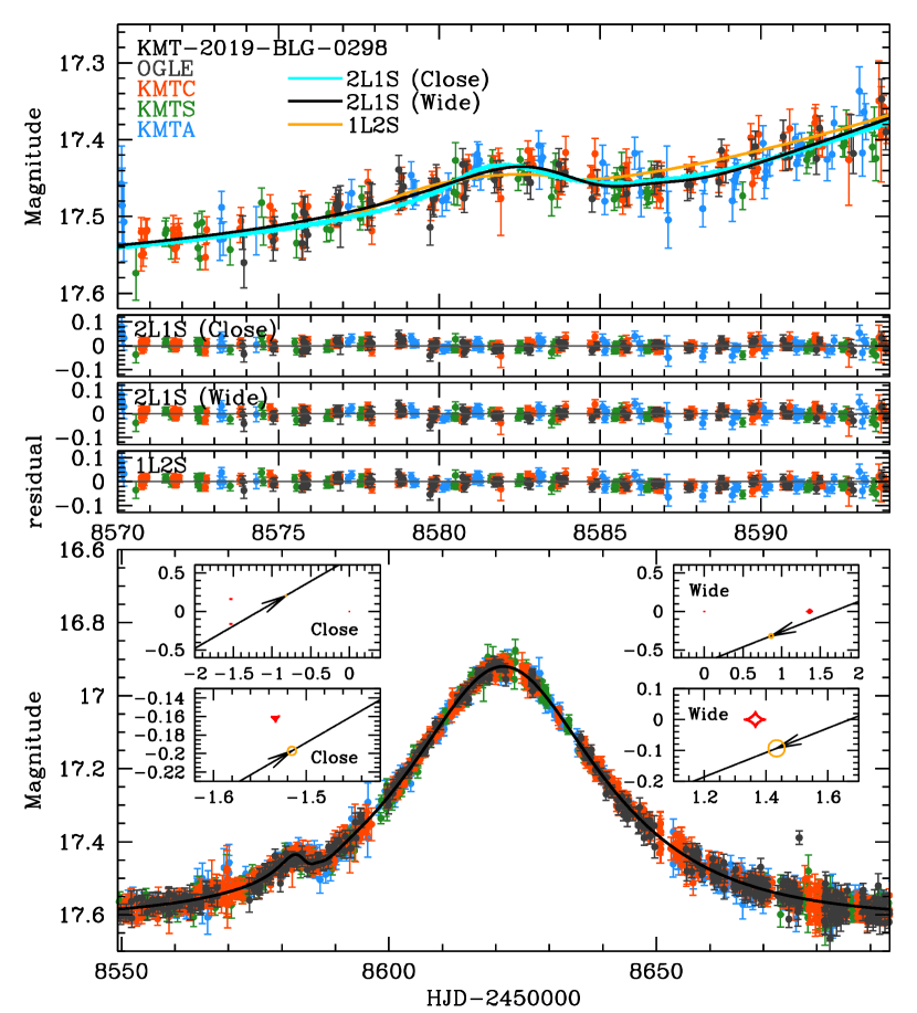
Figure 1: Data (color-coded by observatory) together with the predictions and residuals for the two planetary models of KMT-2019-BLG-0298 specified in Table 2, plus the 1L2S model. The caustic topologies are shown in the insets for both the close and wide geometries, but the wide geometry is decisively favored by $\Delta\chi^{2}=19$. The 1L2S model is excluded at $\Delta\chi^{2}=125$.

Figure 1 shows a low-amplitude $(\Delta I\simeq~{}0.5)$ microlensing event, peaking at $t_{0}=8621.4$ and punctuated by a smooth bump at $t_{\rm anom}\simeq 8582.$, i.e., $-39.4$ days before peak. Assuming that the source is unblended (as is reasonable for such a bright source), the remaining Paczyński (1986) parameters are $u_{0}=0.60$ and $t_{\rm E}=28\,$days. Then $\tau_{\rm anom}=-1.41$ and $u_{\rm anom}=1.53$. Because the source is bright (so, large), while the caustics are likely to be small (because $u_{\rm anom}>1$), we consider that the bump could be due to either a major-image or minor-image perturbation. For these, Equation (2) predicts $s^{\dagger}_{+}=2.02$ and $\alpha=158^{\circ}$, and $s^{\dagger}_{-}=0.49$ and $\alpha=338^{\circ}$, respectively.

The grid search returns two solutions, whose refinements are shown in Table 2. The wide solution is substantially preferred by $\Delta\chi^{2}=19$. For this solution, the heuristic prediction of $\alpha$ is confirmed, while the fit value of $s=s_{\rm outer}=1.89$ indicates that there could be another solution near $s_{\rm inner}=(s^{\dagger}_{+})^{2}/s_{\rm outer}=2.16$. As a matter of due diligence, we seed an MCMC with this value and indeed find a local minimum at $s_{\rm inner}=2.22$. However, this solution is ruled out at $\Delta\chi^{2}=205$, which confirms its failure to be detected in the grid search. The reasons that the degeneracy is decisively broken in this case is that the inner/outer degeneracy is most severe for angles $\alpha=\pm 90^{\circ}$ (Zhang et al., 2022), whereas in this case $\alpha=(90+68)^{\circ}$.

Although, there is no signature of finite-source effects in the light curve (i.e., all values $\rho<0.046$ are consistent at $1\,\sigma$), the absence of a signal actually places significant constraints: $\rho<0.061$ at $2\,\sigma$ and $\rho<0.077$ at $3\,\sigma$. That is, sufficiently larger sources would be impacted by the caustic. See the inset in Figure 1. Hence, when we carry out a Bayesian analysis in Section 5.1, we will ultimately incorporate a $\rho$-envelope function to represent this constraint. For the present, however, we simply note that, in light of the source-radius estimate $\theta_{*}=6.1\,\mu{\rm as}$ derived in Section 4.1, the $1\,\sigma$ range corresponds to Einstein radii, $\theta_{\rm E}>0.13\,{\rm mas}$ and lens-source relative proper motions, $\mu_{\rm rel}>1.7\,{\rm mas}\,{\rm yr}^{-1}$. These values imply that while there is no compelling reason to believe that $\theta_{\rm E}$ is large, it could be relatively large, e.g., $\theta_{\rm E}\sim 0.75\,{\rm mas}$ and still be consistent with the typical range of microlensing proper motions, $\mu_{\rm rel}\lesssim 10\,{\rm mas}\,{\rm yr}^{-1}$. If so, this would favor a nearby lens and thus a potentially large (hence, measurable) microlens parallax, $\pi_{\rm E}$.

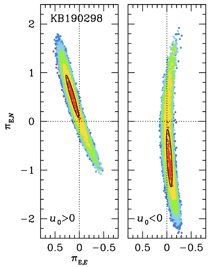
Figure 2: Scatter plot on the ${\mbox{\boldmath$\pi$}}_{\rm E}$ plane derived from the MCMC of the two parallax models of KMT-2019-BLG-0298 presented in Table 2, color coded (red, yellow, green, cyan, blue) for $\Delta\chi^{2}<(1,4,9,16,25)$. The contours are effectively 1-D, with widths $\sigma(\pi_{{\rm E},\parallel})\equiv\sigma_{\parallel}\sim 0.039$ and 0.046. The black contours show the mean and covariances ($\Delta\chi^{2}=1$) that are used in Section 5.1.

Therefore, as a matter of due diligence, and despite the relatively short Einstein timescale, $t_{\rm E}=28\,$day, we undertake a parallax analysis. The results, given in Table 2, are consistent with ${\mbox{\boldmath$\pi$}}_{\rm E}=0$, and in this sense the parallax is “undetected”. Nevertheless, as shown in Figure 2, the fit does place 1-dimensional (1-D) constraints on ${\mbox{\boldmath$\pi$}}_{\rm E}$, and we will incorporate these into the Bayesian analysis in Section 5.1. However, because ${\mbox{\boldmath$\pi$}}_{\rm E}$ is poorly constrained in the orthogonal direction, the free fit allows for $\pi_{\rm E}$ values that would be very unlikely in a posterior fit. These would unphysically broaden the errors in $q$ and other parameters. We note that (except for $u_{0}$), all the parameter values from the parallax fits are consistent with those from the standard fits at $1\,\sigma$. Hence, we will finally report $(s,q)$ and the physical parameters that are derived from them based on the standard fit of Table 2.

Because the anomaly is a smooth, featureless bump, we must also consider the possibility that it is due to an extra source, i.e., 1L2S, rather than an extra lens. However, we find that such models are excluded by $\Delta\chi^{2}=125$.

3.3 KMT-2019-BLG-1216

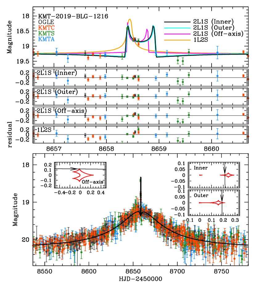
Figure 3: Data (color-coded by observatory) together with the predictions and residuals for the three planetary models of KMT-2019-BLG-1216 specified in Table 3, plus the 1L2S model. The caustic topologies are shown in the insets for the inner, outer, and off-axis models. The first two are perfectly degenerate but the last is decisively disfavored at $\Delta\chi^{2}=24$. The 1L2S model is excluded at $\Delta\chi^{2}=57$.

Figure 3 shows a low-amplitude, generally smooth microlensing event, peaking at $t_{0}=8658.44$, except for 6 elevated points (from 3 observatories) over an interval of 5.2 hours. The maximum extent of the deviation, defined by the two limiting points that lie on the 1L1S curve, is 15.4 hours and is centered at $t_{\rm anom}\simeq 8658.62$, i.e., just $+0.18$ days after peak. A 1L1S fit to the unperturbed parts of the light curve yields $u_{0}=0.18$ and $t_{\rm E}=90\,$days. Then, $\tau_{\rm anom}=+0.002$ and $u_{\rm anom}=0.18$. The first anomalous point is about 0.4 mag brighter than the others and is almost 1 mag brighter than the point that precedes it by 2.3 hours. Therefore, the anomaly is very likely to be a caustic entrance that is followed by a caustic trough, but it is difficult to make a further assessment by eye. Within the heuristic framework of an on-axis (or near-axis) anomaly, Equation (2) predicts $s^{\dagger}_{+}=1.094$ and $\alpha=89.4^{\circ}$.

The grid search returns three solutions, whose refinements are shown in Table 3 and are illustrated in Figure 3. Two of these are a classical inner/outer degeneracy (Gaudi & Gould, 1997), in which (as is often the case, Yee et al. 2021), the outer-solution caustic has a resonant topology, with the source intersecting its “planetary wing”. These two solutions have nearly identical values of $\alpha=89.6^{\circ}$, which are in excellent agreement with the heuristic prediction, and $s^{\dagger}=\sqrt{s_{\rm inner}s_{\rm outer}}=1.094$, which is also in near perfect agreement.

However, there is also a third solution, which has a fully resonant topology, and in which the source intersects an off-axis cusp. As illustrated by Figure 3, the degeneracy of the inner/outer solutions is intrinsic, while the off-axis solution degeneracy is only possible because of a lack of data during the latter part of the caustic perturbation. Nevertheless, because the off-axis solution is disfavored by $\Delta\chi^{2}=24$, we reject it.

As a matter of due diligence, we check for 1L2S solutions, but find that these are rejected by $\Delta\chi^{2}=57$.

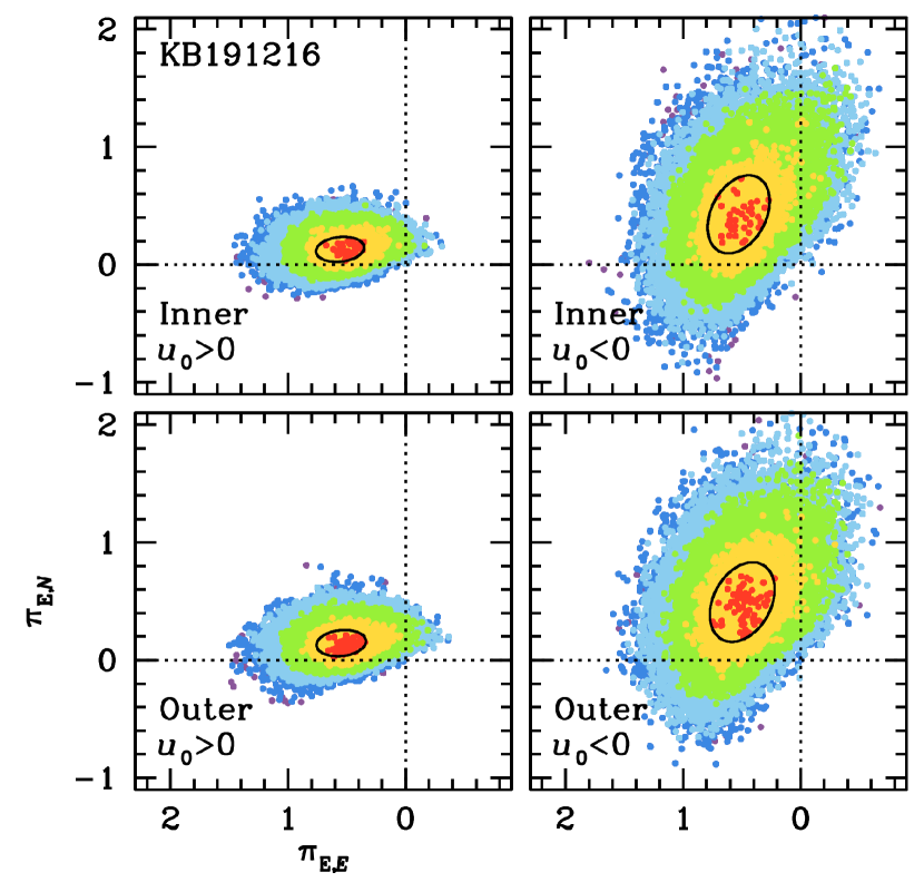
Figure 4: Scatter plot on the ${\mbox{\boldmath$\pi$}}_{\rm E}$ plane derived from the MCMC of the four parallax models of KMT-2019-BLG-1216 presented in Table 4, color coded (red, yellow, green, cyan, blue) for $\Delta\chi^{2}<(1,4,9,16,25)$. The black contours show the mean and covariances ($\Delta\chi^{2}=1$) that are used in Section 5.2.

While $\rho$ is not well measured, there is weak $\chi^{2}$ minimum at $\rho\sim 6\times 10^{-4}$ and a secure $3\,\sigma$ upper limit of $\rho<11\times 10^{-4}$. In Section 4.2, we will show that $\theta_{*}\simeq 0.40\,\mu{\rm as}$. Hence, these $\rho$ values correspond to $\theta_{\rm E}\sim 0.67\,{\rm mas}$ and $\theta_{\rm E}>0.36\,{\rm mas}$. Thus, it is at least plausible that $\theta_{\rm E}$ is relatively large, which would be consistent with a nearby lens and so a relatively large (hence, measurable) microlens parallax $\pi_{\rm E}=\pi_{\rm rel}/\theta_{\rm E}$. Therefore, despite the faintness of the source, we attempt a parallax analysis. The results are shown in Table 4 and illustrated in Figure 4.

We will approach this ${\mbox{\boldmath$\pi$}}_{\rm E}$ measurement cautiously. While there is no reason to doubt this measurement based on the modeling, the best-fit values of $\pi_{\rm E}$ are relatively large, and the improvement is only $\Delta\chi^{2}=10.5$ for 4 degrees of freedom (dof). Even assuming Gaussian statistics, this has false alarm probability of $p=(1+\Delta\chi^{2}/2)\exp(-\Delta\chi^{2}/2)=3\%$.

Our orientation toward such a measurement depends on our prior expectation on the magnitude of $\pi_{\rm E}$. For a typical microlensing event, the expected value is much closer to zero, and the fraction of events with such large $\pi_{\rm E}$ values is small. In such conditions, a $p=3\%$ measurement cannot be considered compelling: in addition to the relatively high false-alarm probability, the large parallax could be due to systematics. However, KMT-2019-BLG-1216 is far from typical: it has an exceptionally large $t_{\rm E}$ and there is evidence for a possibly large $\theta_{\rm E}$. Therefore, we will begin the Bayesian analysis in Section 5.2 by examining the posterior distributions in the absence of the ${\mbox{\boldmath$\pi$}}_{\rm E}$ constraint before deciding whether to incorporate it.

3.4 KMT-2019-BLG-2783

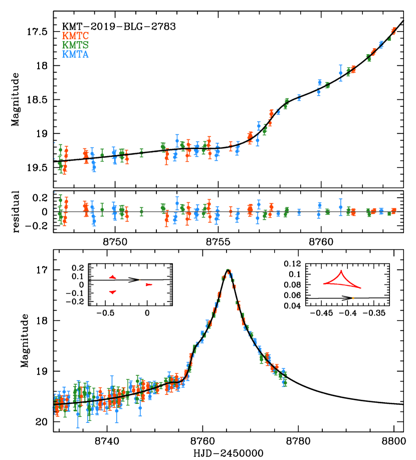
Figure 5: Data (color-coded by observatory) together with the prediction and residuals for the model of KMT-2019-BLG-2783 specified in Table 5. The caustic topology is shown in the insets.

Figure 5 shows a smooth, somewhat complex, perturbation on the rising wing of a microlensing event that peaks at $t_{0}=8764.4$, i.e., close to the end of the season. When this anomaly is excised, a 1L1S fit yields $u_{0}=0.06$ and $t_{\rm E}=24\,$days. The anomaly is characterized by a dip at $t_{\rm anom,dip}\simeq 8756.3$, followed by a bump at $t_{\rm anom,bump}\simeq 8758.0$. If the dip is regarded as the driving feature, then $\tau_{\rm anom,dip}=-0.34$ and $u_{\rm anom}=0.34$, $s^{\dagger}_{-}=0.84$ and $\alpha_{-}=350^{\circ}$, while if the bump is regarded as the driving feature, then $\tau_{\rm anom,bump}=-0.27$ and $u_{\rm anom}=0.27$, $s^{\dagger}_{+}=1.14$ and $\alpha_{+}=168^{\circ}$. In either case, if the heuristic prediction is correct, then the non-driving feature (bump or dip, respectively) would have to be naturally explained by the resulting geometry.

In fact, the grid search returns only a single solution whose refinement is shown in Table 5. The $s^{\dagger}_{-}$ prediction is qualitatively confirmed, while the $\alpha$ prediction is off by $\sim 10^{\circ}$. The $s^{\dagger}_{-}$ inaccuracy derives from the difficulty in judging the exact position of the dip in the presence of the bump. As can be seen from Figure 5, the error in the $\alpha$ estimate is due to the generic problem that minor-image caustics lie off-axis, which is exacerbated by the fact that $q$ is large, implying that the separation of the caustics is also large (Han, 2006). As anticipated in the previous paragraph, the bump is then naturally explained by the fact that the source passes close to a cusp as it exits the trough between the two minor-image caustics. Indeed, there is also a bump before the dip, which is much weaker because the source passes much farther from the cusp. This bump is hardly noticeable in the data because of larger error bars, but it can be discerned in the model.

The source passes about 0.015 from the cusp, which creates a $3\,\sigma$ limit, $\rho<0.01$. This is of relatively little interest because, given the estimate $\theta_{*}=0.39\,\mu{\rm as}$ that is derived in Section 4.3, it corresponds to a limit $\mu_{\rm rel}>0.6\,{\rm mas}\,{\rm yr}^{-1}$, which excludes only a small fraction of parameter space. Nevertheless, we will include the constraints on $\rho$ via an envelope function when we carry out the Bayesian analysis in Section 5.3.

Due to the brevity of the event, the faintness of the source, as well as the absence of any data more than 10 days after $t_{0}$, we do not attempt a parallax analysis.

3.5 OGLE-2019-BLG-0249

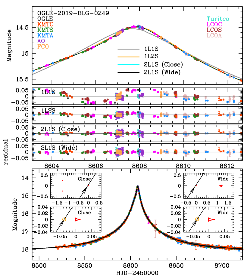
Figure 6: Data (color-coded by observatory) together with the predictions and residuals for the two planetary models of OGLE-2019-BLG-0249 specified in Table 7 with the caustic topologies shown as insets. Also shown are the 1L1S and 1L2S models.

Figure 6 shows a long microlensing event of a relatively bright source that, in the absence of model light curves, might be taken for a 1L1S event. However, the residuals to the 1L1S model clearly show a dip at $t_{\rm anom}=8606.0$, i.e., $\Delta t_{\rm anom}\sim-1.5\,$day before the peak at $t_{0}\simeq 8607.5$. Because the source is bright, it is plausible to guess that it might be unblended. This turns out to be not precisely the case, but proceeding on this assumption, $u_{0}=0.04$ and $t_{\rm E}=58\,$day. Hence, $\tau_{\rm anom}=0.026$, $u_{\rm anom}=0.048$, $s^{\dagger}_{+}=0.976$ and $\alpha=303^{\circ}$. Table 6 shows that the $\alpha$ prediction is accurate to high precision, but $s^{\dagger}=\sqrt{s_{\rm close}s_{\rm wide}}=0.985$ is slightly off. The reason is that the source flux is only about 76% of the baseline flux. This does not affect $\alpha$, which can be written in terms of the invariant $t_{\rm eff}\equiv u_{0}t_{\rm E}$ (for high-magnification events, Yee et al. 2012), as $\tan\alpha=t_{\rm eff}/\Delta t_{\rm anom}$. However, it does affect $s^{\dagger}$, with the 24% blending fraction driving $s^{\dagger}$ about 24% closer to unity.

3.5.1 A Survey+Followup Event

In addition to survey data from OGLE and KMT, OGLE-2019-BLG-0249 was intensively observed by many follow-up observatories (see Figure 6), in part because it was a Spitzer target and in part because it was a moderately-high magnification event ($A_{\rm max}=33$) in a low-cadence field (see Table 1). The current AnomalyFinder series of papers includes the analysis of events only if they are (1) identified as anomalous by the AnomalyFinder algorithm, which is applied to KMT data alone, and (2) have a plausible planetary solution based on survey data alone. This “publication grade” analysis then (3) lays the basis for deciding whether the planet is ultimately included in the complete AnomalyFinder sample. From the standpoint of (2) and (3), it is therefore essential to ask how the event would have been evaluated in the absence of followup data.

Nevertheless, if this evaluation determines that the planet should be in the AnomalyFinder papers and/or if it is included in the final sample, the followup data may be used to improve the characterization of the planet.

OGLE-2019-BLG-0249 is the first planet with extensive followup data to be included in this series, following 7 previous papers containing a total of 37 planets and “possible planets”. There have, of course, been other published planets that had extensive followup data and that will ultimately enter the AnomalyFinder sample. For example, the planetary anomaly in OGLE-2019-BLG-0960 was originally discovered in followup data, and therefore Yee et al. (2021) carefully assessed that this planet could be adequately characterized based on survey data alone. Another relevant example is OGLE-2016-BLG-1195, for which the MOA group obtained intensive data over peak (including the anomaly) by using their survey telescope in followup mode (Bond et al., 2017). In principle, one should assess whether this anomaly would have been adequately characterized had MOA observed at its normal cadence. However, as a practical matter, this is unnecessary because the KMT and Spitzer groups showed that this planet could be adequately characterized based on an independent survey-only data set (Shvartzvald et al., 2017).

3.5.2 Survey-Only Analysis

Thus, we began by analyzing the survey data alone. These results have already been reported above in Table 6, when we compared them to the heuristic predictions. We note that before making these fits, we removed the KMTC points during the two days $|{\rm HJD}^{\prime}-8706|<1$, due to saturation and/or significant nonlinearity of this very bright target. We also checked that if these excluded points were re-introduced, which we do not advocate, the parameters were affected by $\lesssim 2\,\sigma$.

In addition to the two planetary solutions shown in Table 6, there are two local minima derived from the grid search that, when refined, have binary-star mass ratios, i.e., $q\sim 0.15$ and $q\sim 0.25$, with source trajectories passing roughly parallel to a side of a Chang & Refsdal (1979, 1984) caustic (not shown). This is a common form of planet/binary degeneracy for dip-type anomalies (Han & Gaudi, 2008). However, in the present case, these binary solutions are rejected by $\Delta\chi^{2}=64$. See Table 6,

As a matter of due diligence, we also fit the data to 1L2S models. These usually give poor fits to dip-type anomalies, but there can be exceptions. However, in this case, we find that 1L2S is ruled out by $\Delta\chi^{2}=475$.

3.5.3 Followup Data

The followup observations were all, directly or indirectly, initiated in response to an alert that this event would be monitored by Spitzer. Although the Spitzer observations themselves could not begin until 9 July (due to telescope-pointing restrictions), i.e., 66 days after $t_{0}$, OGLE-2019-BLG-0249 was chosen by the Spitzer team on 29 April (6 days before $t_{0}$) in order to “claim” any planets that were discovered (which would also ultimately require that the microlens parallax be measured at sufficient precision). See the protocols of Yee et al. (2015).

On 30 April, the Tsinghua Microlensing Group, working with the Spitzer team, initiated observations on three 1-meter telescopes from the Las Cumbres Observatory at the same locations as the KMT telescopes, which we designate in parallel as LCOC, LCOS, and LCOA, using an SDSS $i$ filter.

Based on these observations, combined with ongoing survey observations by OGLE and KMT, these teams noted that the event was probably anomalous and, on this basis, alerted the microlensing community by email. Because this alert was triggered by an anomaly, such observations can be used only to characterize the planet, but not to “claim” its detection according to the Spitzer protocols (Yee et al., 2015). (However, from Section 3.5.2, we can see that this issue has subsequently become moot.) Four observatories in the Microlensing Follow Up Network ($\mu$FUN), which is composed mainly of small telescopes, responded to this alert, i.e., the (Auckland, Farm Cove, Kumeu, Turitea) observatories, respectively, in (Auckland, Pakuranga, Auckland, Palmerston) New Zealand, with respectively, (0.41, 0.36, 0.41, 0.36) meter mirrors, and respectively, ($R$, white, $R$, $R$) filters.

We found that the Kumeu observations were not of sufficient quality to include them in the analysis. In addition, there were two other observatories, both in Chile, i.e., the Danish 1.5 meter and the SMARTS 1.3 meter, that began observations on May 10 and 11, respectively, i.e., 5–6 days after $t_{0}$. We do not include these observations because they were taken too late to help constrain any of the event parameters.

3.5.4 Survey+Followup Analysis

Table 7 shows the parameters after incorporating the followup data into the fit. The values of $q$ increase by about 10%, corresponding to $\sim 2\,\sigma$, which is not surprising given that the additional data are concentrated on the anomaly. The changes in $s$ are similar. From the comparisons of Tables 6 and 7, the most puzzling (and potentially most consequential) change is that $\rho$ drops by a factor $\sim 2$ without much change in the error bar. We investigate this and find that these three parameters are tightly correlated, which is very plausible given that they are all derived from the same short feature in the light curve, so that the three parameter changes are all expressions of the same additions to the data set.

3.5.5 Parallax Analysis

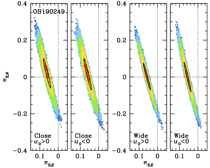
Figure 7: Scatter plot on the ${\mbox{\boldmath$\pi$}}_{\rm E}$ plane derived from the MCMC of the four parallax models of OGLE-2019-BLG-0249 presented in Table 7, color coded (red, yellow, green, cyan, blue) for $\Delta\chi^{2}<(1,4,9,16,25)$. The contours are effectively 1-D, with typical widths $\sigma_{\parallel}\sim 0.0080$ and 0.0065, for the close and wide solutions respectively. The black contours show the mean and covariances that are used in Section 5.4.

Because the event is long ($t_{\rm E}\sim 75\,$day) and reaches relatively high magnification ($A_{\rm max}\sim 30$), and because the source is relatively bright ($I_{S}\sim 18$), it is plausible that substantial parallax information can be extracted. We therefore add four parameters, i.e., ${\mbox{\boldmath$\pi$}}_{\rm E}$ and $\gamma$, and report the results in Table 7. A scatter plot of the MCMC on the ${\mbox{\boldmath$\pi$}}_{\rm E}$ plane is shown in Figure 7 for each of the four solutions. As in the case of KMT-2019-BLG-0298, the contours are essentially 1-D, with axis ratios $\sim 10$. However, contrary to that case, even the long axes of the error ellipses are relatively small, $\sigma_{\perp}\sim 0.08$, which is comparable to the offsets of the 1-D contours from the origin. Hence, the argument given in Section 3.2 for adopting the standard-model parameters (but incorporating the ${\mbox{\boldmath$\pi$}}_{\rm E}$ constraints) does not apply, and we therefore use the full parallax solutions from Table 7 when we carry out the Bayesian analysis in Section 5.4.

3.6 OGLE-2019-BLG-0679

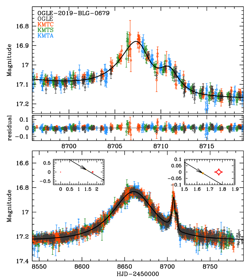
Figure 8: Data (color-coded by observatory) together with the prediction and residuals for the model of OGLE-2019-BLG-0679 specified in Table 8. The caustic topology is shown in the insets.

Figure 8 shows a roughly 10-day bump, which peaks at $t_{\rm anom}\simeq 8707.6$ and is itself punctuated by a shorter 2-day bump on its falling wing, all on the falling wing of a microlensing event that peaks at $t_{0}=8660.7$. When this anomaly is excised, a 1L1S fit (assuming no blending, as is plausible for such a bright source) yields $u_{0}=0.87$ and $t_{\rm E}=31\,$days. Hence, $\tau_{\rm anom}=1.51$, $u_{\rm anom}=1.74$, $s^{\dagger}_{+}=2.20$ and $\alpha=30^{\circ}$.

The grid search returns only one solution, whose refinement is shown in Table 8. The value of $\alpha$ is in good agreement with the heuristic prediction, while the fitted value of $s_{\rm inner}=2.22$ is in “surprising” agreement with $s^{\dagger}_{+}$, given that the anomaly does not appear to be caustic crossing. Figure 8 shows that the solution has an “inner” topology. In fact, if we had used the fit values for $u_{0}$ and $t_{\rm E}$ (as opposed to those assuming no blending), we would have derived $s^{\dagger}=2.13$, which would suggest that there might be another solution at $s_{\rm outer}=(s^{\dagger}_{+})^{2}/s_{\rm inner}=2.04$. However, it is clear from the caustic topology in Figure 8 that the peak of the bump is due to the source passing the on-axis cusp and the shorter, post-peak bump is due to passage of the off-axis cusp. Hence, in a hypothetical “outer” solution, this extra bump would occur before the peak of the main bump. Thus, there is no degeneracy.

Although $\rho$ is not measured, the constraints on $\rho$ are of some interest. That is, we will show in Section 4.5 that $\theta_{*}\sim 7.0\,\mu{\rm as}$, so the $3\,\sigma$ limit, $\rho<0.03$, rules out $\mu_{\rm rel}<2.8\,{\rm mas}\,{\rm yr}^{-1}$, which is a reasonably well populated part of parameter space. We will therefore incorporate the $\rho$ envelope function when we carry out the Bayesian analysis in Section 5.5.

Because the source is relatively bright ($I_{S}\sim 17.3$) and the anomaly is long after the peak and has two features that are separated by 4 days, we attempt a parallax analysis. That is, while in many cases, the change in source trajectory induced by parallax could be compensated (or mimicked) by lens orbital motion, this is much more difficult when the model must accommodate additional light-curve features. See, e.g., An & Gould (2001).

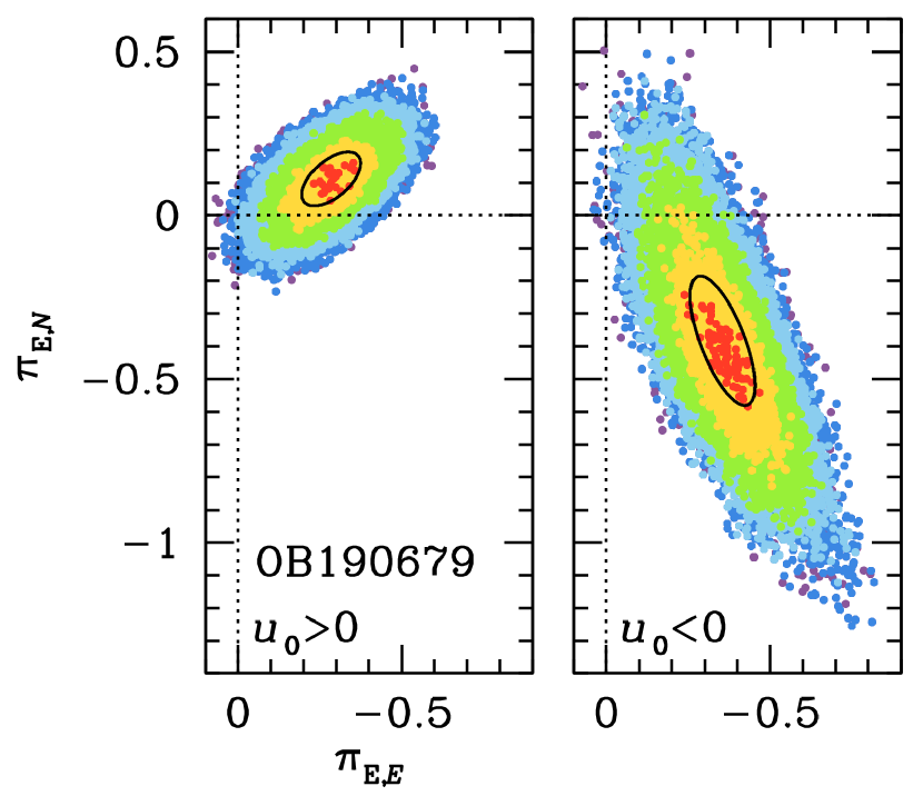
Figure 9: Scatter plot on the ${\mbox{\boldmath$\pi$}}_{\rm E}$ plane derived from the MCMC of the two parallax models of OGLE-2019-BLG-0679 presented in Table 8, color coded (red, yellow, green, cyan, blue) for $\Delta\chi^{2}<(1,4,9,16,25)$. The black contours show the mean and covariances that are used in Section 5.5.

The results are shown in Table 8 and illustrated in the ${\mbox{\boldmath$\pi$}}_{\rm E}$ scatter plot from the MCMC in Figure 9. Including parallax and orbital motion improves the fit $\Delta\chi^{2}=29$. Nevertheless, as we explain in some detail in Section 5.5, we will adopt the standard-model parameters for purposes of this paper. However, we document the details of the parallax fit here in anticipation that they will be useful when the ground-based and space-based parallax fits are later integrated. While we do not know what the space-based parallax fits will reveal, we do note that preliminary reduction of the Spitzer data shows a fall of $\sim 20$ flux units over 37 days, which should be enough to strongly constrain the parallax. In brief, when quoting parameters from this paper, only the “Standard” column in Table 8 should be used.

3.7 OGLE-2019-BLG-0344

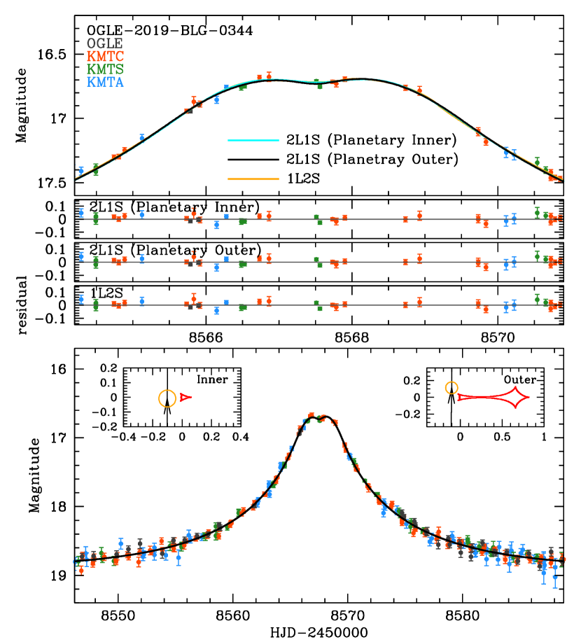
Figure 10: Data (color-coded by observatory) together with the predictions and residuals for the two planetary models of OGLE-2019-BLG-0344 specified in Table 9 as well as the 1L2S model specified in Table 11. All three models can explain the data equally well. In addition, there are 6 other non-planetary 2L1S models, most of which also can explain the data equally well. See Figure 11. Hence, this event cannot be cataloged as “planetary”.

Figure 10 shows a moderately-high magnification microlensing event, peaking at $t_{0}=8567.53$ and punctuated by a short dip that is almost exactly at peak. A 1L1S fit to the data (with the anomaly excluded) yields $u_{0}=0.10$ and $t_{\rm E}=14\,$days. Hence, $\tau_{\rm anom}=0$, $u_{\rm anom}=0.1$, $s^{\dagger}_{-}=0.95$, and $\alpha=270^{\circ}$.

A grid search does indeed return two planetary solutions whose refinements are shown in Table 9 and that are in good agreement with these predictions, i.e., $s^{\dagger}=\sqrt{s_{\rm inner}s_{\rm outer}}=0.95$, and $\alpha=270^{\circ}$. However, it also returns six other solutions. Before discussing these, we first note that the planetary solutions are somewhat suspicious in that they have relatively large values of $\rho\simeq 0.06$. We will show in Section 4.6 that $\theta_{*}\simeq 1.03\,\mu{\rm as}$. If these solutions are correct, they would therefore imply $\theta_{\rm E}=17\,\mu{\rm as}$ and $\mu_{\rm rel}=0.44\,{\rm mas}\,{\rm yr}^{-1}$. The first of these falls in the category of “exciting if true”, while the second has a relatively implausible $p=0.5\%$ probability according to Equation (9). Therefore, we also show for comparison the solutions with $\rho=0$, which are disfavored by $\Delta\chi^{2}=8$.

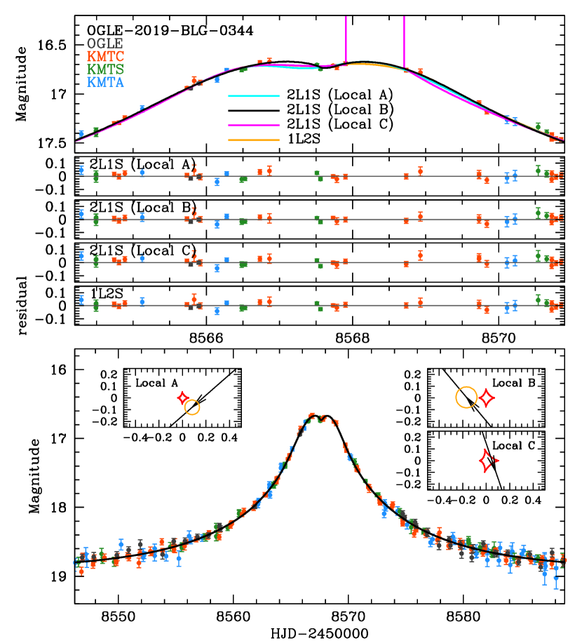
Figure 11: Data (color-coded by observatory) together with the predictions and residuals for the three close-binary models of OGLE-2019-BLG-0344 specified in Table 10, as well as the 1L2S model. Two of the three close-binary models can explain the data about as well as the planetary models. In addition, there are three wide-binary models that are not shown. These viable binary-lens models provide an additional reason that this event cannot be cataloged as “planetary”.

The six other solutions come in three pairs, which each approximately obey the close/wide degeneracy (Dominik, 1999). We label these pairs (A,D), (B,E), and (C,F). The close solutions are given in Table 10 and illustrated in Figure 11. One of these also has an implausibly large $\rho$, so we show the $\rho=0$ solutions in all cases. The bottom line is that if we consider the free $\rho$ case, then Local B is preferred over either planetary solution by $\Delta\chi^{2}=6$, while if we consider the $\rho=0$ case, then Local A is within $\Delta\chi^{2}<1$ of either planetary solution. Hence, there is no reason to believe that the companion is a planet rather than another star. To avoid clutter, we do not present a table or figure for the three wide solutions, but the situation is qualitatively similar.

Finally, we investigate 1L2S models, which are shown in Table 11. In this case, the apparent “dip” is the result of two sources of nearly equal brightness successively passing the lens, with nearly equal impact parameters and with an interval of 2.0 days. The values of $\rho_{1}$ and $\rho_{2}$ are each poorly measured, and if we were to take them at face value, then the two stars would nearly overlap in projection. Hence, we also consider the $\rho_{1}=\rho_{2}=0$ case. This has the best $\chi^{2}$ for any of the $\rho=0$ cases.

We conclude that the lens-source system could be either 1L2S or 2L1S and, if the latter, the lens could equally well be planetary or binary in nature. Hence, we strongly counsel against classifying this event as “planetary.”

3.8 KMT-2019-BLG-0304

In many ways, KMT-2019-BLG-0304 is very similar to OGLE-2019-BLG-344 (Section 3.7), except that the anomaly near peak is a bump rather than a dip. Figure 12 shows a moderately-high magnification microlensing event, peaking at $t_{0}=8574.0$ and punctuated by a short bump at $t_{\rm anom}=8574.5$, i.e. just $\Delta t_{\rm anom}=0.5\,$day after peak. The source is extremely faint, $I_{S}\sim 23$, which implies (e.g., Yee et al. 2012) that in 1L1S and 2L1S fits, the parameter combinations $t_{\rm eff}\equiv u_{0}t_{\rm E}$, $t_{*}\equiv\rho t_{\rm E}$, and $t_{q}\equiv qt_{\rm E}$, will be much better determined than $(u_{0},t_{\rm E},\rho,q)$. For the 1L1S fit, we find $t_{\rm eff}=13.7\,$day. This implies $\alpha=\tan^{-1}(t_{\rm eff}/\Delta t_{\rm anom})=88^{\circ}$, which is independent of $t_{\rm E}$. On the other hand, the prediction for $s^{\dagger}_{+}$ does depend on $t_{\rm E}$. Noting that $u_{\rm anom}=u_{0}/\sin\alpha\simeq u_{0}$, this can be written as

$$s^{\dagger}_{+}={1\over 2}\biggl{(}\sqrt{4+{u_{0}^{2}\over\sin^{2}\alpha}}+{u_{0}\over\sin\alpha}\biggr{)}\rightarrow 1+{u_{0}\over 2}+{u_{0}^{2}\over 8}.$$ (10)

Adopting $t_{\rm E}=165\,$day as a fiducial value, this implies $u_{0}=0.083$, and thus, $s^{\dagger}_{+}=1.04$.

A grid search does indeed return two planetary solutions whose refinements are shown in Table 12, which are in good agreement with these predictions, i.e., $s^{\dagger}=\sqrt{s_{\rm inner}s_{\rm outer}}=1.05$, and $\alpha=88^{\circ}$. In contrast to the case of KMT-2019-BLG-0304, there are no other 2L1S solutions. However, as in that case, there is a competitive 1L2S model, whose parameters are given in Table 13.

At present, there is no way to distinguish between these two solutions. The “free $\rho$” 1L2S solution does predict an unusually low proper motion, $\mu_{\rm rel}\sim 0.2\,{\rm mas}\,{\rm yr}^{-1}$. However, as shown in Table 13, the 1L2S solution remains competitive even when we impose $\rho=0$. In principle, the solutions could be distinguished by measuring the colors of the two sources: because the secondary source is $\sim 3.7$ mag fainter than the primary, it should be substantially redder. However, the event is heavily extincted, $A_{I}\sim 4.4$, so that even the primary source does not yield a good color measurement from the entire event. Hence, measurement of the color of the secondary source, likely 5 mag fainter in the $V$ band, is completely hopeless. Therefore, we strongly counsel against including this event as planetary.

We note that the 2L1S and 1L2S models do predict very different $t_{\rm E}$ and therefore (because $f_{S}t_{\rm E}$ is an invariant), different source fluxes. Hence, it is conceivable that these could be distinguished by measuring the source flux from future adaptive optics (AO) observations on next-generation extremely large telescopes (ELTs). However, we only mention this possibility and do not pursue it in the present context.

4 Source Properties

As in Section 3.1, above, we begin by reproducing (with slight modification) the preamble to Section 4 of Jung et al. (2022). Again, this is done for the convenience of the reader. Readers who are familiar with Jung et al. (2022) may skip this preamble.

If $\rho$ can be measured from the light curve, then one can use standard techniques (Yoo et al., 2004) to determine the angular source radius, $\theta_{*}$ and so infer $\theta_{\rm E}$ and $\mu_{\rm rel}$:

$$\theta_{\rm E}={\theta_{*}\over\rho};\qquad\mu_{\rm rel}={\theta_{\rm E}\over t_{\rm E}}.$$ (11)

However, in contrast to the majority of published by-eye discoveries (but similarly to most of new AnomalyFinder discoveries reported in Zang et al. 2021, 2022, 2023; Hwang et al. 2022; Gould et al. 2022; Jung et al. 2022), most of the planetary events reported in this paper have only upper limits on $\rho$, and these limits are mostly not very constraining. As discussed by Gould et al. (2022), in these cases, $\theta_{*}$ determinations are not likely to be of much use, either now or in the future. Nevertheless, the source color and magnitude measurement that are required inputs for these determinations may be of use in the interpretation of future high-resolution observations, either by space telescopes or AO on large ground-based telescopes (Gould, 2022). Hence, like Gould et al. (2022), we calculate $\theta_{*}$ in all cases.

Our general approach is to obtain pyDIA (Albrow, 2017) reductions of KMT data at one (or possibly several) observatory/field combinations. These yield the microlensing light curve and field-star photometry on the same system. We then determine the source color by regression of the $V$-band light curve on the $I$-band light curve. For the $I$-band source magnitudes, we adopt the values and errors from the parameter tables in Section 3 after aligning the reporting system (e.g., OGLE-IV or KMT pySIS) to the pyDIA system via regression of the $I$-band light curves. While Gould et al. (2022) were able to calibrate the KMT pyDIA color-magnitude diagrams (CMDs) using published field star photometry from OGLE-III (Szymański et al., 2011) or OGLE-II (Szymański, 2005; Kubiak & Szymański, 1997; Udalski et al., 2002), only 3 of the 7 subprime-field events in this paper are covered by these catalogs. Hence, for the remaining 4, we work directly in the KMTC pyDIA magnitude system. Because the $\theta_{*}$ measurements depend only on photometry relative to the clump, they are unaffected by calibration. In the current context, calibration is only needed to interpret limits on lens light. Where relevant, we carry out an alternative approach to calibration.

We then follow the standard method of Yoo et al. (2004). We adopt the intrinsic color of the clump $(V-I)_{0,\rm cl}=1.06$ from Bensby et al. (2013) and its intrinsic magnitude from Table 1 of Nataf et al. (2013). We obtain $[(V-I),I]_{\rm S,0}=[(V-I),I]_{\rm S}+[(V-I),I]_{\rm cl,0}-[(V-I),I]_{\rm cl}$. We convert from $V/I$ to $V/K$ using the $VIK$ color-color relations of Bessell & Brett (1988) and then derive $\theta_{*}$ using the relations of Kervella et al. (2004a, b) for giant and dwarf sources, respectively. After propagating errors, we add 5% in quadrature to account for errors induced by the overall method. These calculations are shown in Table 14. Where there are multiple solutions, only the one with the lowest $\chi^{2}$ is shown. However, the values of $\theta_{*}$ can be inferred for the other solutions by noting the corresponding values of $I_{S}$ in the event-parameter tables and using $\theta_{*}\propto 10^{-I_{S}/5}$. In any case, these are usually the same within the quoted error bars.

Where relevant, we report the astrometric offset of the source from the baseline object.

Comments on individual events follow, where we also note any deviations from the above procedures.

4.1 KMT-2019-BLG-0298

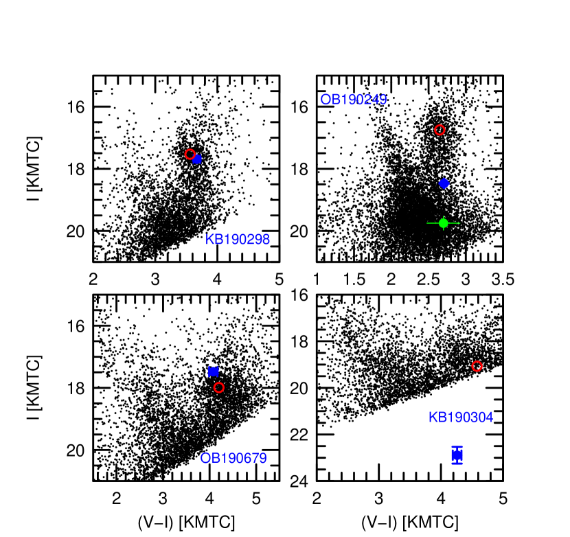
Figure 13: Color-magnitude diagrams for 4 of the 7 events analyzed in this paper, each identified by an abbreviation, e.g., KB190298 for KMT-2019-BLG-0298. The centroid of the red clump and the lens position are always shown in red and blue, respectively. Where relevant, the blended light is shown in green. When there are multiple solutions, we show only the source and blend for the lowest-$\chi^{2}$ solution.

The positions of the source and clump centroid are shown in blue and red respectively in Figure 13 together with the background of neighboring field stars. The blended light is consistent with zero, so it is not represented in the CMD. The source position (derived from difference imaging) is offset from the baseline object by 24 mas, which is consistent with measurement error.

On the other hand, the $1\,\sigma$ error on the blended flux is about 7% of the source flux, which would correspond to $I_{B}\sim 20.4$. According to the KMT website, there are $A_{I}\sim 2.9\,$mag of extinction toward this line of sight, while the mean distance modulus of the bar is 14.30 (Nataf et al., 2013). Hence, a bulge lens star that saturated this $1\,\sigma$ limit would have $M_{I}\sim 3.2$, implying that no useful limit can be placed on flux from the lens.

While the normalized source size is not well measured, it is constrained to be $\rho<0.075$ at $3\,\sigma$. From the values of $\theta_{*}=6.12\,{\rm mas}$ and $t_{\rm E}=27.7\,$day in Tables 14 and 2, we therefore obtain $\theta_{\rm E}>0.082\,{\rm mas}$ and $\mu_{\rm rel}>1.1\,{\rm mas}\,{\rm yr}^{-1}$. As can be seen from Equation (9), this is only marginally constraining. Nevertheless, we will use the $\rho$ envelope function in Section 5.1 to constrain the Bayesian analysis.

Finally, we note that Gaia (Gaia Collaboration et al., 2016, 2018) reports a source proper motion

$${\mbox{\boldmath$\mu$}}_{S}(N,E)=(-5.91\pm 0.41,-4.20\pm 0.64)\,{\rm mas}\,{\rm yr}^{-1}\qquad({\rm Gaia}).$$ (12)

There are two reasons for mild caution regarding this result. First, the same solution yields a $3.6\,\sigma$ negative parallax, $\pi_{S}=-1.696\pm 0.469\,{\rm mas}$. Second, the Gaia RUWE parameter is 1.25. It is extremely unlikely that the large negative parallax is due to normal statistical fluctuations if one interprets the error bars naively. Jung et al. (2022) showed that “high” RUWE numbers are indicative of spurious source proper motions in microlensing events. While, these “high” values were all above 1.7, i.e., far above the RUWE value of 1.25 for KMT-2019-BLG-0298, it is still the case that this RUWE value is somewhat above average. Noting that Rybizki et al. (2022) found that Gaia errors in microlensing fields are typically underestimated by a factor of two, we accept the estimate of Equation (12), but we double the error bars. With this revision, the negative parallax becomes $<2\,\sigma$.

We note that the source is a typical bulge clump giant, both from its proper motion and its position on the CMD.

4.2 KMT-2019-BLG-1216

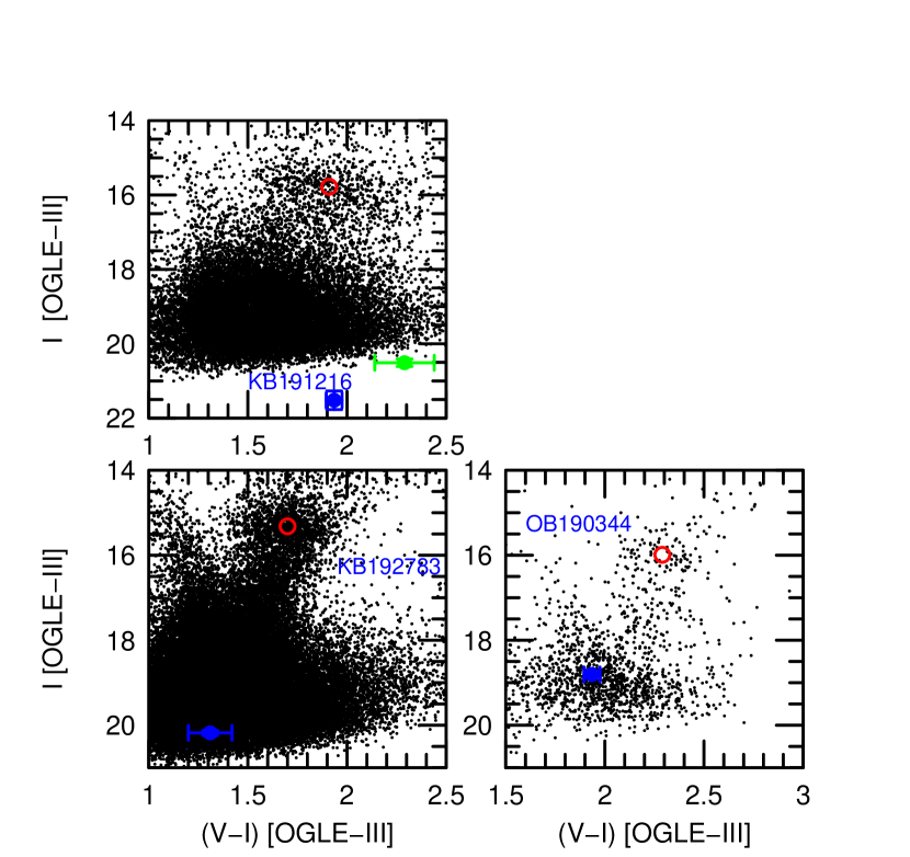
Figure 14: Color-magnitude diagrams for the remaining 3 events analyzed in this paper. See caption of Figure 13.

The positions of the source and clump centroid are shown in blue and red respectively in Figure 14, while the blended light is shown in green.

Our procedures differ substantially from most other events in this paper. First, we do not obtain a reliable source color from regression because the $V$-band signal is too weak. Therefore, to determine the source position on the CMD, it is unnecessary to make use of the pyDIA reductions. Instead, we go directly from the OGLE-IV value and error shown in Table 3 to the calibrated OGLE-III system by finding the $I$-band offset between OGLE-III and OGLE-IV from comparison stars. We then find the offset relative to the clump (Table 14) and infer from this offset the $(V-I)_{S,0}$ intrinsic color using the Hubble Space Telescope (HST) CMD from Baade’s Window (Holtzman et al., 1998).

To find $I_{B}$, we subtract this source flux from the flux of the baseline object in the OGLE-III catalog, $I_{\rm base}=20.15$. Unfortunately, there is no color measurement for this object in the OGLE-III catalog. Therefore, to estimate its color, we first identify its counterpart in the KMTC pyDIA catalog. After transforming the photometry to the OGLE-III system, we find agreement for $I_{\rm base}$ within 0.03 mag. Therefore, we transform the pyDIA $(V-I)_{\rm base}$ into the OGLE-III system and then proceed to find $(V-I)_{B}$ in the usual way.

The baseline object is offset from the source by 120 mas, which means it cannot be the lens, and in fact cannot be dominated by the lens. If there were no errors in the estimates of $I_{\rm base}$ and $I_{S}$, this would imply that the blend flux would place a very conservative upper limit on the lens flux. In fact, $I_{S}$ has a 0.25 mag error from the modeling, although this has only a small effect on $I_{B}$ because $>70\%$ of the baseline light comes from the blend. The error in the DoPhot (Schechter et al., 1993) photometry of the baseline object is of greater concern. While it is encouraging that OGLE-III and KMTC pyDIA agree closely on this measurement, both could be affected by the mottled background of these crowded fields (Park et al., 2004). Therefore, to be truly conservative, we place a limit on the lens flux of twice the inferred blend flux, i.e., $I_{L}>I_{B}-0.75=19.76$.

When calculating $\theta_{*}$, we take account of the correlation between $I_{S,0}$ and $(V-I)_{S,0}$ in the above-described color-magnitude-relation method. That is, at each possible offset (i.e., taking account of the 0.25 mag error in $I_{S}$) we allow for a 0.1 mag spread in $(V-I)_{S,0}$, centered on the value for that $I_{S}$. Then we consider the ensemble of all such estimates within the quoted error of $I_{S}$.

4.3 KMT-2019-BLG-2783

The positions of the source and clump centroid are shown in blue and red respectively in Figure 14. After transforming the source flux to the OGLE-III system and comparing to the OGLE-III baseline object, we find that the blended light is consistent with zero. From the pyDIA analysis, we find that the source is offset from the baseline object by only 14 mas, which is consistent with zero within the measurement errors.

We find that all values of $\rho<(8,12,15)\times 10^{-3}$ are consistent at $(1,2,3)\,\sigma$. Given the value $\theta_{*}=0.39\,{\rm mas}$ from Table 14 and $t_{\rm E}=23.6\,$day from Table 5, these values correspond to $\mu_{\rm rel}>(0.75,0.50,0.40)\,{\rm mas}\,{\rm yr}^{-1}$. These are virtually unconstraining according to Equation (9). Nevertheless, we will include a $\rho$-envelope function in the Bayesian analysis of Section 5.3.

Based on the absence of blended light, we set the limit on lens flux at half the source flux, i.e., $I_{L}>I_{S}+0.75=20.93$.

4.4 OGLE-2019-BLG-0249

The positions of the source and clump centroid are shown in blue and red respectively in Figure 13. The blended light (green) cannot be determined from the KMT pyDIA analysis because there is no true “baseline” during 2019. Rather, we find the blended flux from OGLE-IV and transform to the pyDIA system, $I_{B}=19.75\pm 0.05$. While the source color is determined with high precision from this very bright event, the error in the blend color is very large, $(V-I)_{B}=2.70\pm 0.22$. Nevertheless, the color plays no significant role because, as we will show, the blend is unlikely to be related to the event.

Using a special pyDIA reduction, with a late-season-based template, we find that the source position (derived from difference images) is offset from the baseline object by 53 mas. Taking account of the fact that these late-season images are still magnified by $A\sim 1.06$, this separation should be corrected to $\Delta\theta_{S,\rm base}=56\,{\rm mas}$. This implies that the separation of the source (and so, lens) from the blend is $\Delta\theta_{S,B}=(1+f_{S}/f_{B})\Delta\theta_{S,\rm base}=240\,{\rm mas}$. Hence, on the one hand, it cannot be the lens and is very unlikely to be a companion to either the source or the lens. On the other hand, it lies well within the point-spread function (PSF), so it is undetectable in seeing-limited images.

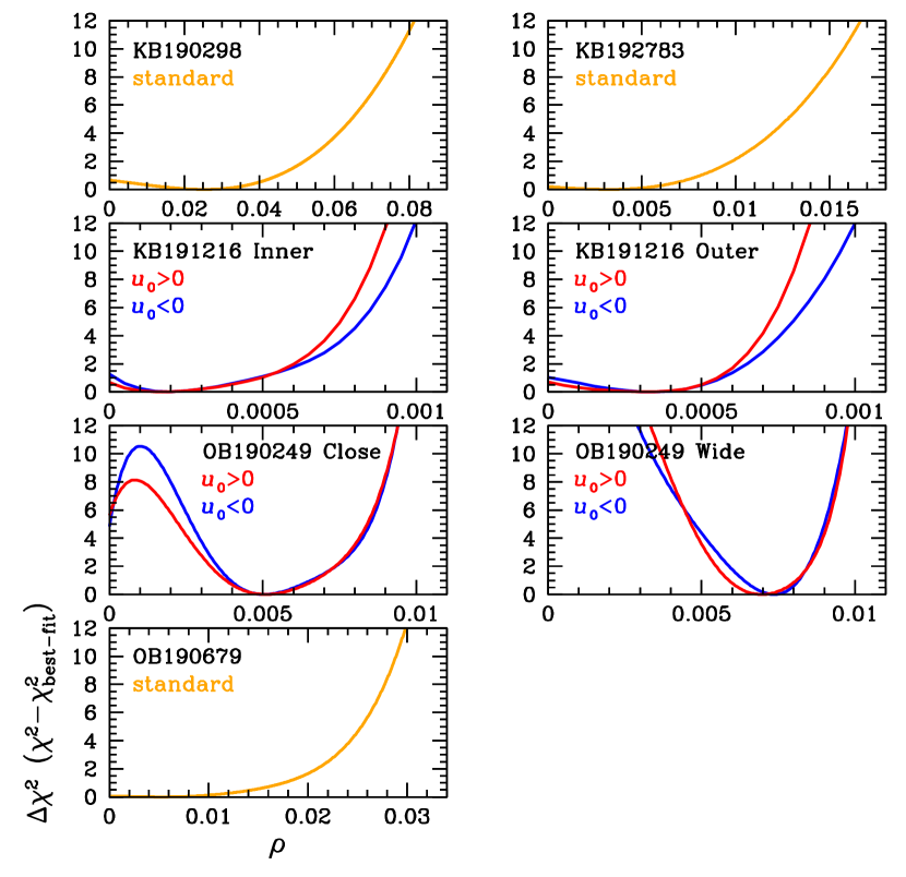
Figure 15: Envelope functions for $\chi^{2}$ versus $\rho$ for all 5 planetary events in this paper.

When ${\mbox{\boldmath$\pi$}}_{\rm E}$ and $\gamma$ are included in the fits, there are well defined minima in $\rho$ for the wide solutions, but less so for the close solutions. See Figure 15. Hence, we will use $\rho$-envelope functions in the Bayesian analysis of Section 5.4 in all cases.

We set the limit on lens flux as that of the blend flux, i.e., $I_{L}>I_{B,\rm Cousins}\simeq I_{B,\rm pyDIA}-0.1=19.65$, where we have estimated (based on other events) a 0.1 mag offset between the pyDIA and standard systems. Note that while it is true that the blend flux could be underestimated due the mottled background of crowded bulge fields, it is also the case that the lens flux can comprise no more than $3/4$ of all the blended flux: otherwise the remaining light would be so far from the source as to be separately resolved.

Finally, we adopt the Gaia proper motion measurement,

$${\mbox{\boldmath$\mu$}}_{S}(N,E)=(-5.29\pm 0.39,-3.92\pm 0.77)\,{\rm mas}\,{\rm yr}^{-1}\qquad({\rm Gaia}),$$ (13)

noting that it has a RUWE value of 1.00.

4.5 OGLE-2019-BLG-0679

The positions of the source and clump centroid are shown in blue and red respectively in Figure 13. According to the better ($u_{0}<0$) solution in Table 8, blended light is detected at $2.5\,\sigma$. For Gaussian statistics, this would have a low false-alarm probability, $p\sim 0.7\%$. Nevertheless, as we now discuss, we treat this detection cautiously.

The key point is that the offset between the source and the baseline object is only 17 mas, which is consistent with zero within the measurement error. This would naturally be explained if there were no blended light or, as a practical matter, much less than is recorded in Table 8. In principle, it might also be explained by the blend being associated with the event, either the lens or a companion to the lens or the source. However, this possibility is itself somewhat problematic. That is, this is a heavily extincted field, $A_{I}=3.8$, so if this blend is behind most of the dust, then $I_{B,0}\sim 15.7$. Hence, if it is in the bulge (e.g., as a companion to the source or as part of the lens system) then it is a giant, i.e., $M_{I}\sim 1.3$. And to be an unevolved main-sequence lens (or companion to the lens), it would have to be at $D_{L}\lesssim 2\,{\rm kpc}$. Of course, this is not impossible, but it is far from typical.

Secondly, there is much experience showing that microlensing photometry does not obey Gaussian statistics, so the $p<1\%$ false-alarm probability cannot be taken at face value. The combination of this reduced confidence with the low prior probability for so much blended light so close to the lens is what makes us cautious about this interpretation. While we adopt the source flux as measured by the fit (i.e., less than the baseline flux), we do not claim to have detected blended light, and therefore we do not show an estimate of the blend in Figure 13.

For both the standard and parallax fits, $\rho$ is poorly constrained. Hence, we will apply the $\rho$-envelope function in the Bayesian analysis of Section 5.5. See Figure 15.

The color measurement, which is tabulated in Table 14 and illustrated in Figure 13, presented some difficulties because the event is low amplitude and suffers heavy extinction. Both factors contribute to low flux variation in the $V$ band. Our usual approach, based on regression of the magnified event in KMTC data, yields $(V-I)_{S}=4.01\pm 0.12$. By comparison, the color of baseline object, which has more than twice the flux of the difference object even at the peak of the event, has an identical central value but substantially smaller error, $(V-I)_{\rm base}=4.01\pm 0.06$. This coincidence of color values would be a natural consequence of the zero-blending hypothesis, but the errors are too large to draw any strong conclusions. Note that both central values place the source $\Delta(V-I)=-0.19$ blueward of the clump.

We made two further efforts to clarify the situation. First, we made independent reductions of KMTS data. These produced a similar color, but with an error bar that was more than twice as large. Combining KMTC and KMTS yields $(V-I)_{S}=4.01\pm 0.11$, which is not a significant improvement.

Second we found the offset from the clump in $(I-H)$, making use of ANDICAM $H$-band data for the light curve and VVV data for the baseline-object and field-star $H$-band photometry. And we compare these to the offsets in $(V-I)$ using the color-color relations of Bessell & Brett (1988). For the baseline object, we find $\Delta(I-H)_{\rm base}=-0.12\pm 0.02$, corresponding to $\Delta(V-I)_{\rm base}=-0.10\pm 0.02$, which is marginally consistent with the direct $V/I$ measurement at $1.4\,\sigma$.

On the other hand, the regression of the $H$-band light curve leads to $\Delta(I-H)_{S}=+0.17\pm 0.06$. This is inconsistent at $4.6\,\sigma$ with the color offset of baseline object. In principle, $\Delta(I-H)$ need not be the same for the source and the baseline because the baseline can have a contribution from blended light of a different color. However, to explain such a large offset from just 15% of the $I$-band light would require an extraordinarily red blend. Considering, in particular, that the blend lies just 1.3 mag below the clump, we consider this to be very unlikely.

In the face of this somewhat contradictory evidence, we adopt $\Delta(V-I)_{S}=-0.12\pm 0.09$. That is, first, given that the baseline light is dominated by the source, it provides the best first guidance to the source color. We then adopt a compromise value between the $V/I$ and $I/H$ determinations that is consistent with both at $\sim 1\,\sigma$. This value is also well within the $1\,\sigma$ interval of the source-color determination in $V/I$. For the error bar, we adopt the offset between these two baseline-object determinations, in recognition of the fact that they disagree by more than $1\,\sigma$. We consider that the $I/H$ determination of the source color is most likely spurious.

Although unsatisfying, any errors in our adopted resolution of this issue do not have significant implications for the results reported in this paper. The source color (as well as the degree of blending) only impact the $\theta_{*}$ determination, and only at $\lesssim 15\%$. This would be of some concern if we had a precise $\rho$ measurement, in which case it would impact $\theta_{\rm E}$ at the same level. However, we basically have only an upper limit on $\rho$, and this fact completely dominates the uncertainty in $\theta_{\rm E}$. We have presented a thorough documentation of this issue mainly for reference, in case it becomes relevant to the interpretation of Spitzer data. That is, when Spitzer data do not cover the peak of the light curve (as appears to be the case for OGLE-2019-BLG-0679), the parallax measurement can sometimes be substantially improved if the Spitzer source flux is independently constrained via a ground-Spitzer color-color relation together with a ground-based color measurement. Hence, a thorough understanding of potential uncertainties in the latter can be of direct relevance.

We do not attempt to place any limit on the lens light. At the $2\,\sigma$ level, $I_{B}>18.8$, which (assuming the blend lies behind most of the dust) corresponds to $I_{B,0}>15.0$, and so is not constraining.

Finally, we note that Gaia reports a proper motion measurement

$${\mbox{\boldmath$\mu$}}_{S}(N,E)=(-6.04\pm 0.28,-6.35\pm 0.51)\,{\rm mas}\,{\rm yr}^{-1}\qquad({\rm Gaia\ DR3}).$$ (14)

However, it also reports a RUWE number, 1.75. Based on a systematic investigation of Gaia proper motions of microlensed sources, Jung et al. (2022) concluded that such high-RUWE measurements were often spurious or, at least, suspicious. In the present case, caution is further indicated by the fact that the Gaia DR2 measurement, ${\mbox{\boldmath$\mu$}}_{S}(N,E)=(-6.98\pm 0.79,-3.42\pm 1.12)\,{\rm mas}\,{\rm yr}^{-1}$, is inconsistent with the DR3 measurement, even though they are based mostly on the same data.

These discrepancies lead us to make our own independent measurement of ${\mbox{\boldmath$\mu$}}_{S}$ based on almost 10 years of OGLE-IV data, which yields,

$${\mbox{\boldmath$\mu$}}_{S}(N,E)=(-5.32\pm 0.37,-8.36\pm 0.16)\,{\rm mas}\,{\rm yr}^{-1}\qquad({\rm OGLE-IV}).$$ (15)

This measurement is strongly inconsistent with the Gaia DR3 measurement, casting further doubt upon the latter. However, as we discuss in Section 5.5, the OGLE-IV measurement is, similar to Gaia DR3, in significant tension with other information about the event.

Therefore, we do not incorporate any ${\mbox{\boldmath$\mu$}}_{S}$ measurement in the Bayesian analysis of Section 5.5. Nevertheless, as we will discuss in that section, the various estimates of ${\mbox{\boldmath$\mu$}}_{S}$ raise enough concerns about the microlensing ${\mbox{\boldmath$\pi$}}_{\rm E}$ measurement as to convince us to report the “Standard” (i.e., non-parallax) solution for our final values.

4.6 OGLE-2019-BLG-0344

As discussed in Section 3.7, this event has planetary solutions, but it cannot be claimed as a planet. Hence, the CMD analysis is presented solely for completeness. Because the source is consistent with being unblended in the planetary fits, we simply adopt the parameters of the OGLE-III baseline object as those of the microlensed source. These are shown as a blue circle in Figure 14, while the source centroid is shown as a red circle.

4.7 KMT-2019-BLG-0304

Due to heavy extinction, the red clump on the CMD is partially truncated by the $V$-band threshold. Therefore, we determine the height of the clump in the $I$-band by matching the pyDIA to the VVV catalog (Minniti et al., 2010, 2017) and then determining the $(V-I)$ color from the portion of the red clump that survives truncation. This is shown as a red circle in Figure 13. We then determine the offset from the clump in the $I$ band (Table 14) and then apply the HST color-magnitude relation, as in Section 4.2. Note that the color of the red clump centroid plays no role in this calculation, and it is shown in Figure 13 only to maintain a consistent presentation with other events.

5 Physical Parameters

To make Bayesian estimates of the lens properties, we follow the same procedures as described in Section 5 of Gould et al. (2022). We refer the reader to that work for details. Below, we repeat the text from Section 5 of Jung et al. (2022) for the reader’s convenience.

In Table 15, we present the resulting Bayesian estimates of the host mass $M_{\rm host}$, the planet mass $M_{\rm planet}$, the distance to the lens system $D_{L}$, and the planet-host projected separation $a_{\perp}$. For the three of the five events, there are two or more competing solutions. For these cases (following Gould et al. 2022), we show the results of the Bayesian analysis for each solution separately, and we then show the “adopted” values below these. For $M_{\rm host}$, $M_{\rm planet}$, and $D_{L}$, these are simply the weighted averages of the separate solutions, where the weights are the product of the two factors at the right side of each row. The first factor is simply the total weight from the Bayesian analysis. The second is $\exp(-\Delta\chi^{2}/2)$ where $\Delta\chi^{2}$ is the $\chi^{2}$ difference relative to the best solution. For $a_{\perp}$, we follow a similar approach provided that either the individual solutions are strongly overlapping or that one solution is strongly dominant. If neither condition were met, we would enter “bi-modal” instead. However, in practice, this condition is met for all 3 events for which there is potentially an issue. Note that in all cases (including those with only one solution), we have provided symmetrized error bars in the “adopted” solution, for simplicity of cataloging. The reader interested in recovering the asymmetric error bars can do so from the table.

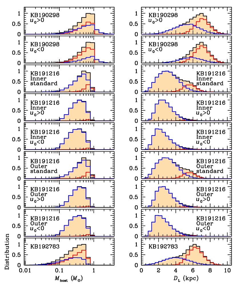
Figure 16: Histograms of the host mass (left) and lens distance (right) for 3 of the 5 unambiguously planetary events, as derived from the Bayesian analysis. Disk (blue) and bulge (red) distributions are shown separately, with their total shown in black.

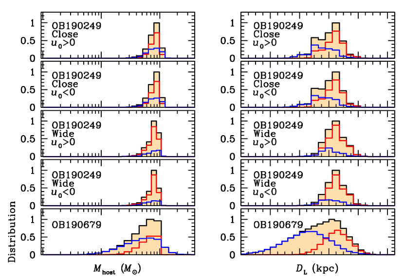
Figure 17: Histograms of the host mass (left) and lens distance (right) for the remaining 2 unambiguously planetary events, as derived from the Bayesian analysis. Disk (blue) and bulge (red) distributions are shown separately, with their total shown in black.

We present Bayesian analyses for 5 of the 7 events, but not for OGLE-2019-BLG-0344 and KMT-2019-BLG-0304, for which we cannot distinguish between competing interpretations of the event. See Sections 3.7 and 3.8. Figures 16 and 17 show histograms for $M_{\rm host}$ and $D_{L}$ for these 5 events.

5.1 KMT-2019-BLG-0298

As discussed in Section 3.2, we accept the event parameters from the standard (7-parameter) solution in Table 2, but incorporate the ${\mbox{\boldmath$\pi$}}_{\rm E}$ constraints from the parallax-plus-orbital-motion solution. Again, the reason for this is that the ${\mbox{\boldmath$\pi$}}_{\rm E}$ constraints are essentially 1-D, so the parallax MCMC explores regions of very high $|{\mbox{\boldmath$\pi$}}_{\rm E}|$, which would be highly suppressed after incorporating Galactic priors.

In the Bayesian analysis, there are four constraints, i.e., on $t_{\rm E}$, ${\mbox{\boldmath$\mu$}}_{S}$, $\rho$, and ${\mbox{\boldmath$\pi$}}_{\rm E}$. The first is $t_{\rm E}=27.71\pm 0.62\,$day from Table 2. The second is ${\mbox{\boldmath$\mu$}}_{S}(N,E)=(-5.91\pm 0.82,-4.20\pm 1.28)\,{\rm mas}\,{\rm yr}^{-1}$ from Section 4.1. The third is given by $\exp(-\Delta\chi^{2}(\rho)/2)$, where $\Delta\chi^{2}(\rho)$ is the envelope function that is shown in Figure 15. For the fourth, we represent the ${\mbox{\boldmath$\pi$}}_{\rm E}$ scatter plots shown in Figure 2 as Gaussian ellipses (also illustrated in this figure) with means and covariance matrices derived from the MCMC. These have central values and error bars similar to those shown in Table 2 (based on medians) and with correlation coefficients 0.95 and 0.60 for the $u_{0}>0$ and $u_{0}<0$ solutions, respectively. They are highly linear structures with minor axes $\sigma_{\parallel}=(0.039,0.046)$ and axis ratios of $\sigma_{\perp}/\sigma_{\parallel}=(11.0,12.3)$ for the respective cases.

The Bayesian estimates (Table 15 and Figure 16) favor $M\sim 0.7\,M_{\odot}$ hosts that are in or near the bulge, i.e., small $\pi_{\rm rel}$. This preference is due to the ${\mbox{\boldmath$\pi$}}_{\rm E}$ constraint, which is, effectively, a 1-D structure passing through the origin. Hence, for randomly oriented ${\mbox{\boldmath$\mu$}}_{\rm rel}$ (so ${\mbox{\boldmath$\pi$}}_{\rm E}$), the fraction of surviving simulated events scales $\propto\pi_{\rm E}^{-1}$, while the very weak constraints on $\rho$ (so $\mu_{\rm rel}$), imply that typical $\mu_{\rm rel}\sim 5\,{\rm mas}\,{\rm yr}^{-1}$ are favored, so $\theta_{\rm E}\sim 0.4\,{\rm mas}$. Low $\pi_{\rm E}$ then drives $\pi_{\rm rel}=\pi_{\rm E}\theta_{\rm E}$ to low values, and it drives $M=\theta_{\rm E}/\kappa\pi_{\rm E}$ to the higher range of the available mass function. Nevertheless, the fact that the $(u_{0}>0)$ solution for ${\mbox{\boldmath$\pi$}}_{\rm E}$ closely tracks the direction of Galactic rotation (i.e., $\sim 30^{\circ}$ north through east), combined with the fact that the source is measured to be moving at $\mu_{S}\sim 7.3\,{\rm mas}\,{\rm yr}^{-1}$ at $\sim-145^{\circ}$ (north through east, i.e., almost anti-rotation), permits disk hosts with very small $D_{L}$. See Figure 16.

5.2 KMT-2019-BLG-1216

As discussed in Section 3.3, we adopt a cautious attitude toward incorporating the ${\mbox{\boldmath$\pi$}}_{\rm E}$ measurement. That is, given the relatively high value of $\pi_{\rm E}\sim 0.6$, the $p=3\%$ false-alarm probability of this measurement would be too high to accept it for typical microlensing events, for which $\pi_{\rm E}$ is generally much closer to zero. Therefore, we begin the Bayesian analysis using the standard (7-parameter) solution in Table 3. There are then three constraints, i.e., on $t_{\rm E}$ (from Table 3), on $\rho$ (from the envelope function in Figure 15), and on the lens flux, $I_{L}>19.76$ from Section 5.2. The results are shown in Table 15 and illustrated in Figure 16.

The results favor nearby lenses $D_{L}\sim 3.5\,{\rm kpc}$, corresponding to $\pi_{\rm rel}\sim 0.17\,{\rm mas}$. The reason is that while $\rho$ is not measured, it is constrained at, e.g., $2\,\sigma$ to be $\rho\lesssim 8.5\times 10^{-4}$, corresponding to $\theta_{\rm E}>0.47\,{\rm mas}$. Because this is a long event, this threshold corresponds to $\mu_{\rm rel}>1.9\,{\rm mas}$, which is moderately low. Hence, somewhat bigger $\theta_{\rm E}$ are favored by Galactic kinematics, e.g., $\theta_{\rm E}\sim 0.8\,{\rm mas}$, which would also correspond to the weak minimum of the $\rho$-envelope function. Considering the “effective top” of the mass function $M\lesssim 1\,M_{\odot}$, these values respectively imply $\pi_{\rm rel}\gtrsim 0.03\,{\rm mas}$ and $\pi_{\rm rel}\gtrsim 0.08\,{\rm mas}$. For $M\sim 0.5\,M_{\odot}$, i.e., closer to the peak of the mass function, these values are doubled. Hence, nearby lenses are strongly favored, while a broad range of masses is permitted.

The Bayesian results do not give any reason to be suspicious of the ${\mbox{\boldmath$\pi$}}_{\rm E}$ measurement. The main takeaway from Figure 16 is that despite the powerful Galactic priors favoring bulge lenses (e.g., Batista et al. 2011), which tend to “override” the $\rho$ constraint, disk lenses are strongly favored. It is notable that the direction of ${\mbox{\boldmath$\pi$}}_{\rm E}$, for ($u_{0}<0$), is consistent with that of Galactic rotation at $1\,\sigma$. While the central value of this solution, $\pi_{\rm E}=0.7\pm 0.2$, is substantially higher than would be naively indicated by the Bayesian analysis, the error is large. Therefore we incorporate this result.

We find that the main effect of incorporating the ${\mbox{\boldmath$\pi$}}_{\rm E}$ measurement is to effectively eliminate the bulge and near-bulge lenses, which (as explained above) were previously allowed due to the Galactic priors “overriding” the $\rho$ constraint.

5.3 KMT-2019-BLG-2783

There is only one solution, upon which there are three constraints, i.e., on $t_{\rm E}=23.6\,$day (from Table 5), on $\rho$ (from the envelope function in Figure 15), and on the lens flux, $I_{L}>20.93$ from Section 4.3. However, given that the $2\,\sigma$ limit, $\rho<0.011$, corresponds to $\mu_{\rm rel}>0.5\,{\rm mas}\,{\rm yr}^{-1}$, the $\rho$ constraint effectively plays no role. On the other hand, the lens-flux constraint, combined with the low extinction ($A_{I}\sim 0.73$, see Table 14) eliminates solar-type lenses even in the bulge, and then progressively eliminates increasingly less massive stars for increasingly nearby disk lenses. The net result is that the Bayesian results are compatible with a very broad range of distances, but a mass distribution that is sharply curtailed at the high end. See Figure 16.

5.4 OGLE-2019-BLG-0249

There are four solutions (two parallax solutions for each of the close and wide topologies), on which there are five constraints, i.e., on $t_{\rm E}$, $\rho$, $I_{L}$, ${\mbox{\boldmath$\mu$}}_{S}$ and ${\mbox{\boldmath$\pi$}}_{\rm E}$. The first comes from Table 7, the second from the $\rho$-envelope functions discussed in Section 4.4 and shown in Figure 15, the third is $I_{L}>19.65$ (from Section 4.4), and the fourth is from Gaia (Equation (13)). Finally, we characterize the ${\mbox{\boldmath$\pi$}}_{\rm E}$ constraints as 2-D Gaussian distributions, whose $\Delta\chi^{2}=1$ contours are shown as black ellipses in Figure 7. These have central values and error bars similar to those shown in Table 7 (based on medians) and with correlation coefficients (0.91,0.92,0.95,0.94) for the (close, $u_{0}>0$; close, $u_{0}<0$; wide, $u_{0}>0$; wide, $u_{0}<0$) solutions, respectively. They are highly linear structures with minor axes $\sigma_{\parallel}=(0.0080,0.0079,0.0064,0.0067)$ and axis ratios of $\sigma_{\perp}/\sigma_{\parallel}=(9.9,11.0,12.0,12.1)$ for the respective cases.

The result is that the host is very well constrained to be an upper main-sequence star that is in or near the bulge. See Table 15 and Figure 17. The reason that these constraints are much tighter than for any other event analyzed in this paper is that, while neither $\theta_{\rm E}$ nor (the vector) ${\mbox{\boldmath$\pi$}}_{\rm E}$ is well measured, both $\theta_{\rm E}$ and (the scalar) $\pi_{\rm E}$ are reasonably well constrained.

In the case of $\theta_{\rm E}$, the $\rho$-envelope functions have relatively broad, but nonetheless well-defined, minima. It is true that these functions turn over for $\rho\lesssim 0.001$ for the close solution. However, these values typically result in masses $M\gtrsim 5\,M_{\odot}$, and so are excluded by the mass function. Regarding ${\mbox{\boldmath$\pi$}}_{\rm E}$, despite the high axis ratios mentioned above, the (scalar) $\pi_{\rm E}$ are well constrained (and to very similar values) in the four cases because the lines from the origin that are perpendicular to these linear structures all pass though the $1\,\sigma$ contour, with $\sigma_{\perp}\simeq\pi_{{\rm E},\rm best}$.

5.5 OGLE-2019-BLG-0679

As foreshadowed in Sections 3.6 and 4.5, we ultimately decided to report final results (for this paper) based on the “Standard” solution of Table 8. We detail our reasons for this decision at the end of this subsection.

Hence, there is only one solution on which there are two constraints , i.e., on $t_{\rm E}$, and $\rho$. The first comes from Table 8, and the second comes from the $\rho$-envelope function discussed in Section 4.5 and shown in Figure 15.

Table 15 and Figure 17 show that the posterior distributions of both mass and distance are very broad, and the lens system can almost equally well reside in the bulge or disk. This is a consequence of the fact that the only measured constraint is $t_{\rm E}$, while $\theta_{\rm E}$ effectively has only a lower limit.

We made the decision to adopt the “Standard” solution as follows. We first carried out Bayesian analyses for both the “Standard” and “Parallax” solutions to understand how they differ not only with respect to the parameters that we normally report (in Table 15) and display (in Figure 17) but also for the source proper motion, ${\mbox{\boldmath$\mu$}}_{S}$, which is normally considered a nuisance parameter. Before continuing, we note that including the parallax measurement somewhat reduced the estimates of the host mass and distance but left broad distributions for both.

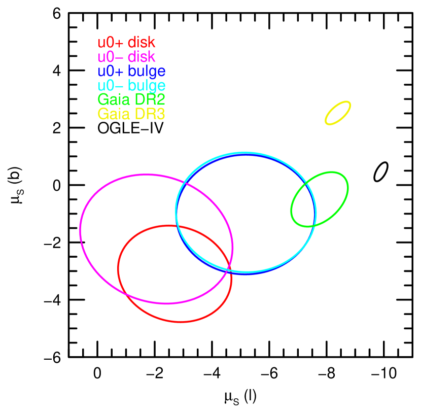
Figure 18: Comparison of the posterior distributions of ${\mbox{\boldmath$\mu$}}_{S}$ for OGLE-2019-BLG-0679, for four classes of model (as indicated in the legend) to the Gaia DR2, Gaia DR3, and OGLE-IV measurements of the same quantity. In particular, Gaia DR3 and OGLE-IV are both in strong tension with all the other error ellipses, including Gaia DR2.

We found that, regardless of which solution ($u_{0}>0$ or $u_{0}<0$) was correct, and regardless of whether the host was assumed to be in the disk or the bulge, both the Gaia DR3 and OGLE-IV measurements of ${\mbox{\boldmath$\mu$}}_{S}$ were inconsistent at $\gtrsim 2\,\sigma$ with the posterior ${\mbox{\boldmath$\mu$}}_{S}$ distributions. See Figure 18. These tensions can be understood by considering the example of disk lenses in the $u_{0}>0$ solution (red), for which $\pi_{{\rm E},b}\simeq 0.3\pm 0.1$. Because ${\mbox{\boldmath$\mu$}}_{\rm rel}$ and ${\mbox{\boldmath$\pi$}}_{\rm E}$ have the same direction, this implies that $\mu_{{\rm rel},b}$ should also be positive. As the prior distributions of ${\mbox{\boldmath$\mu$}}_{{\rm hel},S}$ and ${\mbox{\boldmath$\mu$}}_{{\rm hel},L}$ are basically symmetric in $b$, while ${\mbox{\boldmath$\mu$}}_{{\rm rel},{\rm hel}}={\mbox{\boldmath$\mu$}}_{{\rm hel},L}-{\mbox{\boldmath$\mu$}}_{{\rm hel},S}$, the posterior distributions are driven to positive and negative values for the lenses and sources, respectively.

This “conflict” may well have a perfectly reasonable explanation. As discussed in Section 4.5, the Gaia DR3 measurement may simply be wrong, as signaled both by its high RUWE number and its strong disagreement with both Gaia DR2 and OGLE-IV. See Figure 18. Similarly, the OGLE-IV measurement may be wrong. Alternatively, it may be that either Gaia DR3 or OGLE-IV is correct (or basically correct), that the host lies in the bulge (blue and cyan ellipses), and that the event characteristics are $2\,\sigma$ outliers. In addition, it could be that the ${\mbox{\boldmath$\pi$}}_{\rm E}$ measurement suffers from unrecognized systematics. Given that any of these three explanations is possible in principle, that they can lead to very different results, and that the matter will probably be resolved within a year by the Spitzer parallax measurement, the most prudent course is to defer judgment until the Spitzer data can be properly evaluated. This course will also minimize the possibility that confusion will propagate though the literature.

5.6 OGLE-2019-BLG-0344

Because there is no compelling reason to believe that the planetary solution is correct, we do not present a Bayesian analysis.

5.7 KMT-2019-BLG-0304

Because there is no compelling reason to believe that the planetary solution is correct, we do not present a Bayesian analysis.

6 Discussion

We have analyzed here all 5 of the previously unpublished planets found by the KMT AnomalyFinder algorithm toward the 21 KMT subprime fields. We also analyzed the two events that have nonplanetary solutions, but are consistent with planetary interpretations. Such events are rarely published, but they are a standard feature of the AnomalyFinder series because they can be important for understanding the statistical properties of the sample as a whole. A total of 5 such events were previously published from the 2018 season (Gould et al., 2022; Jung et al., 2022).

6.1 Summary of All 2019 Subprime AnomalyFinder Planets

Table 16 shows these 5 planets and 2 “possible planets” in the context of the ensemble of all such 2019 subprime AnomalyFinder events. The horizontal line distinguishes between objects that we judge as likely to enter the final statistical sample and those that we do not. Note that among the latter, OGLE-2019-BLG-1470 is definitely planetary in nature, but it has a factor $\sim 3$ discrete degeneracy in its mass ratio, $q$. On the other hand, KMT-2019-BLG-0414 has an alternate, orbiting binary-source (xallarap) solution that is disfavored by only $\Delta\chi^{2}=4$, and so it cannot be claimed as a planet.

Thus, of the 11 events (containing 12 planets) that are “above the line”, almost half are published here. This is the main accomplishment of the present work. Among these 5 planets, none is truly exceptional in its own right, although OGLE-2019-BLG-0679 has a relatively large normalized projected separation, $s=2.18$. Indeed, among the 53 previously published (or summarized) AnomalyFinder planets from 2018 and 2019 (Gould et al., 2022; Jung et al., 2022; Zang et al., 2022, 2023), only one had a larger separation, i.e., OGLE-2018-BLG-0383, with $s=2.45$ (Wang et al., 2022).

6.2 2018+2019 Planets: 4 Discrete Characterizations

Because the AnomalyFinder planets for the 2019 prime fields (Zang et al., 2022), as well as all of the 2018 fields (Gould et al., 2022; Jung et al., 2022), have previously been published (or summarized), our work permits several types of comparison between different seasons, different classes of planets, and different methods and conditions of discovery. At the highest level we can compare the 2018 and 2019 seasons in terms of number of planets found by field type (prime versus subprime), method of discovery (by-eye versus AnomalyFinder), source trajectory (caustic crossing or not caustic crossing), and type of perturbation (major image, minor image, or central caustic). Table 17 presents these comparisons and summaries.

6.2.1 Statistical Consistency of 2018 and 2019

The first point is that the 2018 and 2019 seasons are consistent with respect to all of these breakdowns. For example, there were 33 and 25 total detections, respectively, i.e., a difference of $8\pm\sqrt{58}$ according to Poisson statistics. Of all the various comparisons that one could make among the various subcategories, the most “discrepant” is in the difference between the fraction of events identified by the AnomalyFinder, 52% versus 37%, i.e., a difference of $15\%\pm 13\%$, according to binomial statistics. Similarly, the fraction of planets found via major versus minor image perturbations: 55% versus 42%, i.e., a difference of $13\%\pm 14\%$.

Combining five tests, i.e., the Poisson test of total detections and the 4 binomial tests of Table 14, we find $\chi^{2}=3.37$ for 5 dof.

6.2.2 AnomalyFinder Yielded 40% of All Detections

Given that the two seasons are statistically consistent, we should ask what can be learned from their combined statistics. In particular, with 58 planets, this is a factor more than 2.5 times larger than any other homogeneously detected planetary microlensing sample (Suzuki et al., 2016). Perhaps the most striking feature of Table 17 is that 23 of the 58 planets (40%) were initially identified by AnomalyFinder, despite the fact that KMT’s publicly available data (the same as are input to AnomalyFinder) had previously been systematically searched by several experienced modelers. This may indicate the difficulty of by-eye searches in the era of massive microlensing data sets. It also shows that samples derived from by-eye searches alone are not even approximately complete.

At the same time, AnomalyFinder has not replaced by-eye searches: the two actually work hand-in-hand. AnomalyFinder typically identifies of order 250 candidates (after human review of a much larger candidate list) that each requires detailed investigation to various levels. The first step in these massive reviews is to consult the summaries of systematic by-eye investigations, particularly those of C. Han, thereby reducing the number that require new or additional investigations by a factor 3–5. The by-eye searches also serve as a check on the AnomalyFinder completeness. In fact, for 2021, we deliberately accelerated the by-eye searches with three new “mass production” papers (Ryu et al., 2022, 2023; Shin et al., 2023), as well as many other papers on individual planets (see Ryu et al. 2023 for a list), so that about 18 planets that are suitable for statistical studies were identified and prepared for publication prior to running the AnomalyFinder algorithm.

In contrast to the other three statistical indicators that are discussed below, the AnomalyFinder fraction of planets depends on a human factor. For example, when the 2016-2017 data are analyzed, the fraction could go down simply because there has been more time to apply the by-eye approach. And, going forward, the rate could go down because humans have learned more about planetary signatures based on the results from 2018-2019. On the other hand, the rate could go up if humans become less diligent, knowing that the planets will “eventually” be found anyway.

6.2.3 50%$\pm$7% of Planets Have Caustic Crossings

Zhu et al. (2014) predicted that for about half of the planets detected in a KMTNet-like survey, the source would cross a caustic. These crossings are important because they allow the normalized source radius, $\rho$, to be measured, which in turn enables measurement of $\theta_{\rm E}$ and $\mu_{\rm rel}$. In addition to helping to characterize the planet, these measurements allow one to predict when the source and lens will be sufficiently separated to resolve them using AO on large telescopes, which can lead to measurements of the host and planet masses and the system distance. The 2018-2019 AnomalyFinder statistical sample confirms this prediction of Zhu et al. (2014) at relatively high statistical precision.

We note that a large minority of planetary events that do not have caustic crossing nevertheless yield good $\rho$ measurements because the planet is detected when the source passes over a magnification“ridge” that extends from the tip of a cusp. See, for example, OGLE-2016-BLG-1195 (Bond et al., 2017; Shvartzvald et al., 2017). Gould (2022) showed, based on a larger (but inhomogeneous) sample of 102 planetary events, which substantially overlaps the current one, that about 2/3 yield $\rho$ measurements, even though only about 1/2 have caustic crossings.

Of the five planetary events analyzed in the present work, only one (KMT-2019-BLG-1216) has a caustic crossing. Yet, due to inadequate data over the caustic, $\rho$ is not well measured. This problem is likely to be much more common in subprime fields, particularly those that (like KMT-2019-BLG-1216) have cadences of $\Gamma=0.4\,{\rm hr}^{-1}$. None of the 4 planetary events that lacked caustic crossings yielded precise $\rho$ measurements, although for OGLE-2019-BLG-0249, $\rho$ was reasonably well constrained.

6.2.4 50%$\pm$7% of Major/Minor Image Perturbations Are Major

It has long been known that for microlensing events with high, or even moderate, sensitivity to planets, the $(\log s,\log q)$ sensitivity diagrams are nearly symmetric about zero in $\log s$. One aspect of this symmetry is understood at a very deep level, while another aspect remains, to the best of our knowledge, completely unexplored.

Griest & Safizadeh (1998) showed that, for low $q$, there is a deep symmetry in the lens equation for $s\leftrightarrow s^{-1}$ in the immediate neighborhood of the host (or, more accurately, the “center of magnification”). For example, the very first planet to exhibit such a degeneracy, OGLE-2005-BLG-071 (Udalski et al., 2005), has nearly identical $\chi^{2}$ for the two solutions (Dong et al., 2009a). Hence, because the magnification pattern is nearly identical for the two cases, a given source trajectory will generate very similar light curves, and hence nearly equal detectabilities. As a result, all published sensitivity diagrams for high-magnification events (whose planet sensitivity is completely dominated by the source passage close to the center of magnification), are nearly perfectly symmetric. See, for example, OGLE-2007-BLG-050 (Batista et al., 2009) and OGLE-2008-BLG-279 (Yee et al., 2009).

By contrast, for source trajectories that pass closer to the planetary caustics than to the central caustics, the magnification structures, and hence the resulting light-curve morphologies, are completely different. Major images generally have much larger caustics that are flanked by narrow magnification ridges, while minor images have smaller caustic pairs that are threaded by broad magnification troughs. Because of these two very different morphologies, one might expect the symmetry in the sensitivity profiles to break down.

In the very first systematic study of such sensitivity, Gaudi et al. (2002) presented $(\log s,\log q)$ plots for 43 microlensing events. Despite the fact that they span a very broad range of peak magnifications, many of these events display rough symmetry in their sensitivity profiles. However, in detail, many individual events also have an asymmetry in the minimum detectable $\log q$ for $\pm\log s$, with more sensitivity for $\log s<0$. On the other hand, their Figure 13, which combines the sensitivities of these 43 events, shows a slight deviation from symmetry toward positive $\log s$. However, they do not comment upon either effect.

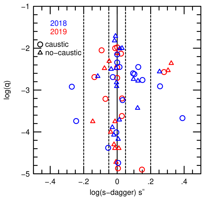
Figure 19: Scatter plot of $\log s^{\dagger}$ versus $\log q$ for 58 AnomalyFinder planets from 2018 and 2019. Here, $s^{\dagger}_{\pm}=(\sqrt{u_{\rm anom}+4}\pm u_{\rm anom})/2$, $u_{\rm anom}$ is the lens-source separation normalized to $\theta_{\rm E}$ at the time of the anomaly, and the “$\pm$” refers to major and minor image perturbations, respectively. A majority of detections have $|\log s^{\dagger}|<0.05$ (inner dashed lines), for which the same light-curve morphology can almost equally be generated by positive or negative $\log s$, including with large absolute values. Hence, there is no correspondence between the signs of $\log s^{\dagger}$ and $\log s$ in this regime. By contrast, for $|s^{\dagger}|>0.2$ (outer dashed lines), the anomalies are generally associated with the planetary caustics, so that $\log s^{\dagger}$ and $\log s$ have the same sign. In this regime there is suggestive evidence (6 versus 2 detections) that there is more overall senstivity to wide separation planets.

Here, we investigate detections in the 2018-2019 AnomalyFinder sample from the standpoint of image perturbations rather than planet-host separation. As will become clear, these represent orthogonal perspectives. Figure 19 shows a scatter plot of $\log q$ versus $\log s^{\dagger}$, for which positive and negative values correspond to major-image and minor-image perturbations, respectively. See Equation (2).

There are three notable features. First, a majority (35/58) of the planets lie within $|\log s^{\dagger}|<0.05$. In this regime, there is essentially no correlation between the signs of $\log s^{\dagger}$ and $\log s$ because either light-curve morphology can almost equally be generated by $s>1$ and $s<1$ lens geometries. The fact that a majority of detections lie in this narrow zone simply reflects the well-known fact that planet sensitivity is higher for relatively high (Gould & Loeb, 1992; Abe et al., 2013) and very high (Griest & Safizadeh, 1998) magnification events. Note that, in this regime, $u_{\rm anom}\simeq(\ln 100)|\log s^{\dagger}|$, so $u_{\rm anom}<0.23$, i.e., $A_{\rm anom}>4.4$. Nevertheless, it is still of interest that the detections are about equally distributed between positive and negative values in this inner zone. That is, the light-curve morphologies are generally very different for positive and negative $\log s^{\dagger}$ (perturbations of the major and minor images), but apparently this leads to very similar planet sensitivities. This question could be investigated to much higher precision based on already existing (or future) planet-sensitivity studies by subdividing the simulations according to $\alpha$ into those with perturbations of the major or minor image.

The second notable feature is that for $|\log s^{\dagger}|>0.2$ (outer dashed lines), there are substantially more (6 versus 2) major-image than minor-image planets. In this regime, the anomalies are generally closely associated with the planetary caustics (and this is so for all 8 cases from Figure 19). Moreover, both of the minor-image perturbations are caustic-crossing, whereas this is the case for only half of the major-image perturbations. Because of small-number statistics, no strong conclusions can be drawn from either of these two comparisons. However, both conform to our naive impression that for planets that are far from the Einstein ring, it should be easier to detect the isolated bump due to a wide-separation planet than the weak dip of a close-separation planet, unless the source actually interacts with one of the two small caustics. Again this issue can be more precisely explored from detailed simulations than from current planet samples, due to small-number statistics.

The third notable feature is that in the intermediate region, i.e., the transition between the central-caustic and the planetary-caustic regimes, there are about an equal number (7 versus 8) of major-image and minor-image perturbations. This suggests that in this regime, the substantially different light-curve morphologies lead to about equal sensitivity. This is again deserving of systematic study via simulations. One might also note that all but one of the major-image perturbations in this regime are from 2018, while all but two of the minor-image perturbations are from 2019, However, as we cannot imagine any physical cause for this near dichotomy, we ascribe it to the random “noticeable effects” that one often discovers when viewing scatter plots.

6.2.5 55%$\pm$7% of Detections Are From Prime Fields

KMT devotes approximately half of its observing time to the 6 prime fields and the other half to the 21 subprime fields. While there are many considerations that go into this division, such as sensitivity to the Galactic distribution of planets, probing planets in a broad range of mass ratios, and probing other types of dim or dark objects like black holes, one consideration is certainly “return of planets on observing-time investment”. Prior to the start of KMT’s commissioning observations in 2015, Henderson et al. (2014) had already shown that there would be diminishing returns from concentrating all observations on the “most productive” fields. This understanding, as well as the experience of OGLE, which pioneered a multi-tiered observing approach, contributed to KMT adopting this strategy. Thus, it is of some interest that the planet return is in fact approximately proportional to the invested observing time.

6.3 6-D Distribution

In Figure 20, we show a six-dimensional (6-D) representation of the 58 planets from 2018 and 2019 AnomalyFinder searches that are discussed in this section. It is an update to Figure 14 from Jung et al. (2022) which included the subset of 33 planets from that paper. To recapitulate their description, it includes 2 continuous dimensions (given by the axes) and 4 discrete dimensions that are represented by colors and point types. The abscissa and ordinate are $\log q$ and $I_{S,\rm anom}\equiv I_{S}-2.5\log[A(u_{\rm anom})]$, with the latter being the source brightness in the unperturbed event at the time of the anomaly. The description of the symbols is identical to those of Jung et al. (2022), and they are also given in the legend.

Previously, Jung et al. (2022) had noted a “paucity of by-eye detections of non-caustic-crossing events (open bluish symbols) at low-$q$: i.e., 1 out of 5 for $\log q<-3$ compared to 7 out of 12 for $\log q>-3$”. This trend is strongly confirmed by the larger sample: 2 out of 12 for $\log q<-3$ compared to 9 out of 16 for $\log q>-3$. They also noted that 14 out of their 16 caustic-crossing planets were discovered by eye and that the remaining two were both in prime fields and at low $\log q<-3$. They suggested this was “a regime where machines may do better than people because the relatively weak signals of low-$q$ events are spread out over a greater number of data points.” In the 2019 sample, almost equal numbers of caustic-crossing planets were found by each method, so that total now is 23 out of 29 caustic-crossing planets, i.e., still heavily favoring by-eye detections. Moreover, the other trend is strongly confirmed: now out of 6 AnomalyFinder caustic-crossing planets, none are from subprime fields, and only one had $\log q>-3$. This strengthens the evidence for the Jung et al. (2022) conjecture that machines excel in the high-cadence, low-$q$ regime for caustic-crossing planets.

One feature of this diagram noted by Jung et al. (2022) that is not confirmed is the apparent threshold of AnomalyFinder detection at $I_{S,\rm anom}=18.75$. There had been only one major exception (OGLE-2018-BLG-0962), which has $I_{S,\rm anom}=20.4$. While there are still no detections fainter than this (previous) outlier, The 1.5 magnitudes, $18.75<I_{S,\rm anom}\lesssim 20.25$, are now “filled in” with a total of 10 planets. Thus, $I_{S,\rm anom}\sim 20.25$ now appears to be the detection floor. This will be tested as additional seasons are analyzed in this series.

Table 1: Event Names, Cadences, Alerts, and Locations

Name	$\Gamma\,({\rm hr}^{-1})$	Alert Date	RAJ2000	DecJ2000	$l$	$b$
KMT-2019-BLG-0298	1.0	05 Apr 2019	17:39:30.72	$-27$:38:17.30	$+0.40$	$+1.83$
OGLE-2019-BLG-0445	0.4
KMT-2019-BLG-1216	0.4	11 Jun 2019	17:53:55.35	$-35$:08:11.90	$-4.43$	$-4.69$
OGLE-2019-BLG-1033	0.2
KMT-2019-BLG-2783	1.0	Post Season	17:57:10.06	$-33$:47:18.67	$-2.92$	$-4.59$
OGLE-2019-BLG-0249	0.1	09 Mar 2019	17:41:36.84	$-34$:42:06.30	$-5.35$	$-2.30$
KMT-2019-BLG-0109	0.4
OGLE-2019-BLG-0679	0.1	05 May 2019	17:42:57.70	$-27$:46:22.37	$+0.69$	$+1.11$
KMT-2019-BLG-2688	1.0
OGLE-2019-BLG-0344	0.2	20 Mar 2019	17:23:52.38	$-29$:32:48.59	$-3.08$	$+3.66$
KMT-2019-BLG-0149	0.4
KMT-2019-BLG-0304	1.0	05 Apr 2019	17:41:18.70	$-32$:31:47.82	$-3.54$	$-1.10$

Table 2: Standard & Parallax 2L1S Models for KMT-2019-BLG-0298

Parameters	Close	Wide	Wide	Wide
	Standard	Standard	$u_{0}>0$	$u_{0}<0$
$\chi^{2}_{\rm tot}$/dof	3494.6/3689	3476.0/3689	3474.9/3685	3475.0/3685
$t_{0}$ (${\rm HJD^{\prime}}$)	8621.421 $\pm$ 0.027	8621.337 $\pm$ 0.034	8621.224 $\pm$ 0.060	8621.226 $\pm$ 0.064
$u_{0}$	0.589 $\pm$ 0.018	0.613 $\pm$ 0.020	0.587 $\pm$ 0.028	-0.607 $\pm$ 0.021
$t_{\rm E}$ (days)	28.506 $\pm$ 0.571	27.715 $\pm$ 0.617	27.979 $\pm$ 0.661	27.273 $\pm$ 0.641
$s$	0.491 $\pm$ 0.007	1.892 $\pm$ 0.030	1.845 $\pm$ 0.054	1.857 $\pm$ 0.051
$q$ ($10^{-3}$)	2.143 $\pm$ 0.253	2.485 $\pm$ 0.343	2.883 $\pm$ 0.680	3.004 $\pm$ 0.763
$\langle{\rm log}\,q\rangle$	-2.665 $\pm$ 0.051	-2.603 $\pm$ 0.059	-2.534 $\pm$ 0.101	-2.518 $\pm$ 0.104
$\alpha$ (rad)	5.753 $\pm$ 0.010	2.766 $\pm$ 0.005	2.827 $\pm$ 0.057	-2.855 $\pm$ 0.069
$\rho$ ($10^{-2}$)	1.179 $\pm$ 0.891	2.680 $\pm$ 1.650	3.188 $\pm$ 2.172	3.409 $\pm$ 2.384
$\pi_{{\rm E},N}$			0.537 $\pm$ 0.440	-0.850 $\pm$ 0.590
$\pi_{{\rm E},E}$			0.152 $\pm$ 0.128	-0.049 $\pm$ 0.057
$ds/dt$ (yr-1)			0.047 $\pm$ 0.959	0.143 $\pm$ 1.026
$d\alpha/dt$ (yr-1)			0.196 $\pm$ 0.474	-0.221 $\pm$ 0.563
$f_{\rm S,OGLE}$	1.399 $\pm$ 0.070	1.502 $\pm$ 0.081	1.407 $\pm$ 0.111	1.473 $\pm$ 0.084
$f_{\rm B,OGLE}$	0.022 $\pm$ 0.070	-0.083 $\pm$ 0.081	0.010 $\pm$ 0.111	-0.055 $\pm$ 0.084

Note. — As discussed in Section 3.2, we accept the event parameters from the “Wide Standard” solution for this event, but incorporate the ${\mbox{\boldmath$\pi$}}_{\rm E}$ constraints from the parallax-plus-orbital-motion solutions in the Bayesian analysis of Section 5.1.

Table 3: Standard 2L1S Models for KMT-2019-BLG-1216

Parameters	Inner	Outer	Off-axis
$\chi^{2}_{\rm tot}$/dof	1236.1/1374	1236.3/1374	1260.6/1374
$t_{0}$ (${\rm HJD^{\prime}}$)	8658.443 $\pm$ 0.239	8658.448 $\pm$ 0.235	8660.978 $\pm$ 0.292
$u_{0}$	0.189 $\pm$ 0.036	0.175 $\pm$ 0.036	0.125 $\pm$ 0.007
$t_{\rm E}$ (days)	88.729 $\pm$ 15.031	94.466 $\pm$ 16.881	138.780 $\pm$ 8.103
$s$	1.118 $\pm$ 0.018	1.074 $\pm$ 0.022	0.990 $\pm$ 0.003
$q$ ($10^{-4}$)	2.438 $\pm$ 0.538	2.323 $\pm$ 0.511	84.727 $\pm$ 10.535
$\langle{\rm log}\,q\rangle$	-3.617 $\pm$ 0.099	-3.637 $\pm$ 0.098	-2.066 $\pm$ 0.055
$\alpha$ (rad)	1.561 $\pm$ 0.014	1.561 $\pm$ 0.014	0.013 $\pm$ 0.032
$\rho$ ($10^{-4}$)	4.409 $\pm$ 1.897	4.184 $\pm$ 1.750	1.757 $\pm$ 0.662
$f_{\rm S,OGLE}$	0.044 $\pm$ 0.010	0.040 $\pm$ 0.010	0.025 $\pm$ 0.002
$f_{\rm B,OGLE}$	0.087 $\pm$ 0.010	0.090 $\pm$ 0.009	0.105 $\pm$ 0.002

Table 4: Parallax 2L1S Models for KMT-2019-BLG-1216

Parameters	Inner		Outer
	$u_{0}>0$	$u_{0}<0$	$u_{0}>0$	$u_{0}<0$
$\chi^{2}_{\rm tot}$/dof	1226.3/1370	1226.4/1370	1226.3/1370	1226.5/1370
$t_{0}$ (${\rm HJD^{\prime}}$)	8659.089 $\pm$ 0.345	8659.053 $\pm$ 0.340	8659.115 $\pm$ 0.338	8659.048 $\pm$ 0.325
$u_{0}$	0.110 $\pm$ 0.030	-0.122 $\pm$ 0.035	0.119 $\pm$ 0.035	-0.137 $\pm$ 0.037
$t_{\rm E}$ (days)	137.465 $\pm$ 33.221	134.147 $\pm$ 36.134	129.232 $\pm$ 36.368	120.992 $\pm$ 30.846
$s$	1.083 $\pm$ 0.013	1.086 $\pm$ 0.016	1.037 $\pm$ 0.022	1.047 $\pm$ 0.023
$q$ ($10^{-4}$)	2.264 $\pm$ 0.593	2.197 $\pm$ 0.594	2.209 $\pm$ 0.616	2.319 $\pm$ 0.585
$\langle{\rm log}\,q\rangle$	-3.644 $\pm$ 0.116	-3.661 $\pm$ 0.121	-3.658 $\pm$ 0.120	-3.639 $\pm$ 0.114
$\alpha$ (rad)	1.602 $\pm$ 0.022	-1.600 $\pm$ 0.020	1.603 $\pm$ 0.022	-1.599 $\pm$ 0.020
$\rho$ ($10^{-4}$)	2.537 $\pm$ 1.266	2.696 $\pm$ 1.384	2.772 $\pm$ 1.350	3.089 $\pm$ 1.514
$\pi_{{\rm E},N}$	0.122 $\pm$ 0.101	0.381 $\pm$ 0.299	0.132 $\pm$ 0.103	0.453 $\pm$ 0.316
$\pi_{{\rm E},E}$	0.543 $\pm$ 0.194	0.523 $\pm$ 0.238	0.535 $\pm$ 0.199	0.490 $\pm$ 0.255
$ds/dt$ (yr-1)	-0.010 $\pm$ 0.880	-0.010 $\pm$ 0.920	-0.050 $\pm$ 0.870	0.010 $\pm$ 0.890
$d\alpha/dt$ (yr-1)	0.090 $\pm$ 0.860	-0.190 $\pm$ 0.890	0.050 $\pm$ 0.870	-0.290 $\pm$ 0.910
$f_{\rm S,OGLE}$	0.023 $\pm$ 0.007	0.025 $\pm$ 0.008	0.026 $\pm$ 0.008	0.029 $\pm$ 0.009
$f_{\rm B,OGLE}$	0.108 $\pm$ 0.007	0.106 $\pm$ 0.008	0.106 $\pm$ 0.008	0.102 $\pm$ 0.009

Table 5: Standard 2L1S Model for KMT-2019-BLG-2783

Parameters	Values
$\chi^{2}_{\rm tot}$/dof	2113.9/2103
$t_{0}$ (${\rm HJD^{\prime}}$)	8765.395 $\pm$ 0.037
$u_{0}$	0.057 $\pm$ 0.003
$t_{\rm E}$ (days)	23.669 $\pm$ 1.065
$s$	0.814 $\pm$ 0.007
$q$ ($10^{-3}$)	3.262 $\pm$ 0.762
$\langle{\rm log}\,q\rangle$	-2.483 $\pm$ 0.101
$\alpha$ (rad)	6.277 $\pm$ 0.023
$\rho$ ($10^{-3}$)	5.131 $\pm$ 3.515
$f_{\rm S,KMTC}$	0.138 $\pm$ 0.008
$f_{\rm B,KMTC}$	0.062 $\pm$ 0.007

Table 6: Survey-Only 2L1S Models for OGLE-2019-BLG-0249

Parameters	Planetary		Binary
	Close	Wide	Close	Wide
$\chi^{2}_{\rm tot}$/dof	1672.5/1682	1670.7/1682	1733.2/1682	1751.1/1682
$t_{0}$ (${\rm HJD^{\prime}}$)	8607.442 $\pm$ 0.004	8607.436 $\pm$ 0.004	8607.446 $\pm$ 0.004	8607.488 $\pm$ 0.004
$u_{0}$ ($10^{-3}$)	30.934 $\pm$ 0.288	31.221 $\pm$ 0.290	32.388 $\pm$ 0.341	28.418 $\pm$ 0.245
$t_{\rm E}$ (days)	76.387 $\pm$ 0.624	76.596 $\pm$ 0.618	76.912 $\pm$ 0.615	84.974 $\pm$ 0.689
$s$	0.581 $\pm$ 0.010	1.663 $\pm$ 0.030	0.231 $\pm$ 0.003	5.657 $\pm$ 0.110
$q$ ($10^{-3}$)	5.918 $\pm$ 0.320	6.166 $\pm$ 0.335	153.281 $\pm$ 8.331	247.573 $\pm$ 17.120
$\langle{\rm log}\,q\rangle$	-2.226 $\pm$ 0.023	-2.209 $\pm$ 0.024	-0.813 $\pm$ 0.024	-0.603 $\pm$ 0.030
$\alpha$ (rad)	5.287 $\pm$ 0.003	5.292 $\pm$ 0.003	2.974 $\pm$ 0.005	2.960 $\pm$ 0.004
$\rho$ ($10^{-3}$)	9.635 $\pm$ 1.582	10.692 $\pm$ 1.466	17.631 $\pm$ 0.751	16.683 $\pm$ 0.645
$f_{\rm S,OGLE}$	0.718 $\pm$ 0.007	0.722 $\pm$ 0.007	0.720 $\pm$ 0.007	0.715 $\pm$ 0.007
$f_{\rm B,OGLE}$	0.219 $\pm$ 0.007	0.216 $\pm$ 0.007	0.217 $\pm$ 0.006	0.220 $\pm$ 0.007

Table 7: Survey+Followup 2L1S Models for OGLE-2019-BLG-0249

Parameters	Close			Wide
	Standard	$u_{0}>0$	$u_{0}<0$	Standard	$u_{0}>0$	$u_{0}<0$
$\chi^{2}_{\rm tot}$/dof	2101.7/2081	1828.1/2077	1828.2/2077	2100.7/2081	1831.4/2077	1831.4/2077
$t_{0}$ (${\rm HJD^{\prime}}$)	8607.430 $\pm$ 0.003	8607.415 $\pm$ 0.011	8607.414 $\pm$ 0.011	8607.426 $\pm$ 0.003	8607.807 $\pm$ 0.017	8607.805 $\pm$ 0.019
$u_{0}$ ($10^{-3}$)	31.133 $\pm$ 0.269	30.859 $\pm$ 0.366	-30.911 $\pm$ 0.369	31.363 $\pm$ 0.277	39.021 $\pm$ 0.490	-39.064 $\pm$ 0.512
$t_{\rm E}$ (days)	75.628 $\pm$ 0.585	76.264 $\pm$ 0.645	76.309 $\pm$ 0.687	75.923 $\pm$ 0.597	76.592 $\pm$ 0.598	76.649 $\pm$ 0.647
$s$	0.554 $\pm$ 0.004	0.543 $\pm$ 0.010	0.545 $\pm$ 0.010	1.753 $\pm$ 0.014	1.777 $\pm$ 0.014	1.775 $\pm$ 0.015
$q$ ($10^{-3}$)	6.643 $\pm$ 0.195	7.461 $\pm$ 0.270	7.455 $\pm$ 0.268	6.983 $\pm$ 0.214	7.819 $\pm$ 0.229	7.805 $\pm$ 0.237
$\langle{\rm log}\,q\rangle$	-2.177 $\pm$ 0.013	-2.127 $\pm$ 0.015	-2.127 $\pm$ 0.016	-2.156 $\pm$ 0.013	-2.106 $\pm$ 0.013	-2.107 $\pm$ 0.013
$\alpha$ (rad)	5.295 $\pm$ 0.002	5.298 $\pm$ 0.012	-5.298 $\pm$ 0.012	5.302 $\pm$ 0.003	5.302 $\pm$ 0.004	-5.302 $\pm$ 0.005
$\rho$ ($10^{-3}$)	5.138 $\pm$ 1.308	5.925 $\pm$ 1.231	6.084 $\pm$ 1.197	6.375 $\pm$ 1.057	7.369 $\pm$ 0.803	7.413 $\pm$ 0.804
$\pi_{{\rm E},N}$		0.016 $\pm$ 0.076	0.008 $\pm$ 0.082		-0.003 $\pm$ 0.068	-0.005 $\pm$ 0.075
$\pi_{{\rm E},E}$		0.061 $\pm$ 0.019	0.059 $\pm$ 0.020		0.056 $\pm$ 0.019	0.056 $\pm$ 0.018
$ds/dt$ (yr-1)		-0.339 $\pm$ 0.688	-0.249 $\pm$ 0.744		0.048 $\pm$ 0.528	0.051 $\pm$ 0.527
$d\alpha/dt$ (yr-1)		0.419 $\pm$ 1.419	-0.569 $\pm$ 1.469		-0.002 $\pm$ 0.303	-0.026 $\pm$ 0.308
$f_{\rm S,OGLE}$	0.727 $\pm$ 0.007	0.719 $\pm$ 0.008	0.720 $\pm$ 0.008	0.730 $\pm$ 0.007	0.724 $\pm$ 0.007	0.724 $\pm$ 0.007
$f_{\rm B,OGLE}$	0.211 $\pm$ 0.006	0.218 $\pm$ 0.007	0.218 $\pm$ 0.007	0.208 $\pm$ 0.006	0.213 $\pm$ 0.007	0.213 $\pm$ 0.007

Table 8: Standard & Parallax 2L1S Models for OGLE-2019-BLG-0679

Parameters	Standard	$u_{0}>0$	$u_{0}<0$
$\chi^{2}_{\rm tot}$/dof	4194.4/4438	4164.9/4434	4163.2/4434
$t_{0}$ (${\rm HJD^{\prime}}$)	8660.604 $\pm$ 0.056	8660.775 $\pm$ 0.085	8660.766 $\pm$ 0.075
$u_{0}$	0.831 $\pm$ 0.016	0.804 $\pm$ 0.026	-0.817 $\pm$ 0.027
$t_{\rm E}$ (days)	32.608 $\pm$ 0.469	33.252 $\pm$ 0.734	32.939 $\pm$ 0.729
$s$	2.216 $\pm$ 0.023	2.161 $\pm$ 0.034	2.167 $\pm$ 0.035
$q$ ($10^{-3}$)	4.785 $\pm$ 0.146	4.072 $\pm$ 0.508	3.837 $\pm$ 0.395
$\langle{\rm log}\,q\rangle$	-2.319 $\pm$ 0.013	-2.387 $\pm$ 0.049	-2.410 $\pm$ 0.044
$\alpha$ (rad)	0.537 $\pm$ 0.003	0.551 $\pm$ 0.011	-0.570 $\pm$ 0.017
$\rho$ ($10^{-3}$)	9.204 $\pm$ 6.906	19.579 $\pm$ 7.847	17.335 $\pm$ 8.553
$\pi_{{\rm E},N}$		0.108 $\pm$ 0.078	-0.398 $\pm$ 0.192
$\pi_{{\rm E},E}$		-0.293 $\pm$ 0.087	-0.358 $\pm$ 0.101
$ds/dt$ (yr-1)		0.368 $\pm$ 0.413	0.554 $\pm$ 0.332
$d\alpha/dt$ (yr-1)		0.177 $\pm$ 0.193	-0.369 $\pm$ 0.205
$f_{\rm S,OGLE}$	1.824 $\pm$ 0.067	1.729 $\pm$ 0.106	1.766 $\pm$ 0.109
$f_{\rm B,OGLE}$	0.203 $\pm$ 0.067	0.295 $\pm$ 0.106	0.255 $\pm$ 0.109

Note. — As discussed in Section 3.6, we adopt the “Standard” parameters for this event.

Table 9: Planetary Models for OGLE-2019-BLG-0344

Parameters	Inner		Outer
	free $\rho$	$\rho=0$	free $\rho$	$\rho=0$
$\chi^{2}_{\rm tot}$/dof	1612.8/1621	1620.2/1622	1612.1/1621	1619.9/1622
$t_{0}$ (${\rm HJD^{\prime}}$)	8567.532 $\pm$ 0.014	8567.529 $\pm$ 0.014	8567.533 $\pm$ 0.014	8567.528 $\pm$ 0.013
$u_{0}$	0.103 $\pm$ 0.005	0.102 $\pm$ 0.004	0.103 $\pm$ 0.005	0.103 $\pm$ 0.005
$t_{\rm E}$ (days)	14.413 $\pm$ 0.470	14.108 $\pm$ 0.366	14.578 $\pm$ 0.496	14.227 $\pm$ 0.426
$s$	0.621 $\pm$ 0.044	0.540 $\pm$ 0.015	1.459 $\pm$ 0.114	1.696 $\pm$ 0.069
$q$ ($10^{-2}$)	2.374 $\pm$ 0.528	2.958 $\pm$ 0.457	2.567 $\pm$ 0.601	3.058 $\pm$ 0.584
$\langle{\rm log}\,q\rangle$	-1.627 $\pm$ 0.096	-1.530 $\pm$ 0.067	-1.595 $\pm$ 0.102	-1.526 $\pm$ 0.083
$\alpha$ (rad)	4.714 $\pm$ 0.023	4.706 $\pm$ 0.021	4.713 $\pm$ 0.022	4.713 $\pm$ 0.025
$\rho$ ($10^{-2}$)	5.809 $\pm$ 1.166		6.269 $\pm$ 1.097
$f_{\rm S,OGLE}$	0.365 $\pm$ 0.021	0.380 $\pm$ 0.018	0.365 $\pm$ 0.021	0.388 $\pm$ 0.019
$f_{\rm B,OGLE}$	0.063 $\pm$ 0.021	0.048 $\pm$ 0.018	0.062 $\pm$ 0.021	0.040 $\pm$ 0.019

Table 10: Close Binary-Star Models for OGLE-2019-BLG-0344

Parameters	Local A		Local B		Local C
	free $\rho$	$\rho=0$	free $\rho$	$\rho=0$	free $\rho$	$\rho=0$
$\chi^{2}_{\rm tot}$/dof	1617.2/1621	1620.7/1622	1605.9/1621	1626.1/1622	1637.8/1621	1637.9/1622
$t_{0}$ (${\rm HJD^{\prime}}$)	8567.444 $\pm$ 0.019	8567.450 $\pm$ 0.016	8567.687 $\pm$ 0.027	8567.616 $\pm$ 0.021	8568.157 $\pm$ 0.025	8568.166 $\pm$ 0.026
$u_{0}$	0.113 $\pm$ 0.006	0.110 $\pm$ 0.005	0.125 $\pm$ 0.005	0.111 $\pm$ 0.006	0.049 $\pm$ 0.002	0.048 $\pm$ 0.002
$t_{\rm E}$ (days)	13.916 $\pm$ 0.389	13.846 $\pm$ 0.361	13.794 $\pm$ 0.367	13.697 $\pm$ 0.380	13.771 $\pm$ 0.320	13.764 $\pm$ 0.328
$s$	0.315 $\pm$ 0.013	0.301 $\pm$ 0.007	0.362 $\pm$ 0.017	0.302 $\pm$ 0.010	0.462 $\pm$ 0.011	0.467 $\pm$ 0.010
$q$	0.527 $\pm$ 0.162	0.515 $\pm$ 0.135	0.804 $\pm$ 0.168	1.841 $\pm$ 0.824	0.333 $\pm$ 0.025	0.329 $\pm$ 0.025
$\langle{\rm log}\,q\rangle$	-0.273 $\pm$ 0.131	-0.288 $\pm$ 0.116	-0.079 $\pm$ 0.079	0.281 $\pm$ 0.173	-0.474 $\pm$ 0.032	-0.480 $\pm$ 0.032
$\alpha$ (rad)	2.412 $\pm$ 0.035	2.419 $\pm$ 0.028	3.999 $\pm$ 0.037	3.882 $\pm$ 0.061	1.245 $\pm$ 0.016	1.248 $\pm$ 0.016
$\rho$ ($10^{-2}$)	4.936 $\pm$ 2.014		8.504 $\pm$ 0.539		0.114 $\pm$ 0.103
$f_{\rm S,OGLE}$	0.397 $\pm$ 0.020	0.399 $\pm$ 0.019	0.412 $\pm$ 0.018	0.412 $\pm$ 0.018	0.360 $\pm$ 0.011	0.360 $\pm$ 0.011
$f_{\rm B,OGLE}$	0.031 $\pm$ 0.020	0.029 $\pm$ 0.018	0.016 $\pm$ 0.017	0.016 $\pm$ 0.017	0.069 $\pm$ 0.011	0.068 $\pm$ 0.011

Table 11: 1L2S Models for OGLE-2019-BLG-0344

Parameters	free $\rho$	$\rho=0$
$\chi^{2}_{\rm tot}$/dof	1609.7/1620	1613.7/1622
$t_{0,1}$ (${\rm HJD^{\prime}}$)	8566.544 $\pm$ 0.071	8566.528 $\pm$ 0.069
$t_{0,2}$ (${\rm HJD^{\prime}}$)	8568.511 $\pm$ 0.069	8568.506 $\pm$ 0.065
$u_{0,1}$	0.082 $\pm$ 0.006	0.077 $\pm$ 0.004
$u_{0,2}$	0.092 $\pm$ 0.012	0.080 $\pm$ 0.005
$t_{\rm E}$ (days)	15.215 $\pm$ 0.440	15.394 $\pm$ 0.430
$\rho_{1}$ ($10^{-2}$)	4.432 $\pm$ 2.775
$\rho_{2}$ ($10^{-2}$)	7.721 $\pm$ 3.885
$q_{\rm F}$	1.032 $\pm$ 0.189	1.054 $\pm$ 0.180
$f_{\rm S,OGLE}$	0.328 $\pm$ 0.015	0.320 $\pm$ 0.014
$f_{\rm B,OGLE}$	0.101 $\pm$ 0.015	0.108 $\pm$ 0.014

Table 12: 2L1S Standard Models for KMT-2019-BLG-0304

Parameters	Close		Wide
	free $\rho$	$\rho=0$	free $\rho$	$\rho=0$
$\chi^{2}_{\rm tot}$/dof	2394.3/2387	2394.9/2388	2393.8/2387	2394.8/2388
$t_{0}$ (${\rm HJD^{\prime}}$)	8574.014 $\pm$ 0.346	8574.020 $\pm$ 0.361	8574.019 $\pm$ 0.341	8574.039 $\pm$ 0.327
$u_{0}$	0.083 $\pm$ 0.024	0.098 $\pm$ 0.048	0.099 $\pm$ 0.029	0.093 $\pm$ 0.030
$t_{\rm E}$ (days)	166.981 $\pm$ 45.725	144.948 $\pm$ 62.216	140.494 $\pm$ 38.089	151.043 $\pm$ 45.234
$s$	0.713 $\pm$ 0.033	0.722 $\pm$ 0.052	1.546 $\pm$ 0.051	1.569 $\pm$ 0.051
$q$ ($10^{-2}$)	1.220 $\pm$ 0.340	1.415 $\pm$ 0.445	1.494 $\pm$ 0.422	1.496 $\pm$ 0.435
$\langle{\rm log}\,q\rangle$	-1.917 $\pm$ 0.122	-1.863 $\pm$ 0.138	-1.838 $\pm$ 0.139	-1.828 $\pm$ 0.127
$\alpha$ (rad)	1.536 $\pm$ 0.025	1.537 $\pm$ 0.024	1.538 $\pm$ 0.024	1.536 $\pm$ 0.023
$\rho$ ($10^{-3}$)	1.667 $\pm$ 1.008		1.954 $\pm$ 1.211
$f_{\rm S,KMTC}$	0.009 $\pm$ 0.003	0.011 $\pm$ 0.006	0.011 $\pm$ 0.004	0.010 $\pm$ 0.003
$f_{\rm B,KMTC}$	0.180 $\pm$ 0.002	0.177 $\pm$ 0.004	0.176 $\pm$ 0.002	0.177 $\pm$ 0.002
$t_{\rm eff}(u_{0}t_{\rm E})$	14.098 $\pm$ 0.796	14.581 $\pm$ 1.025	14.393 $\pm$ 0.887	14.492 $\pm$ 0.820
$t_{*}(\rho t_{\rm E})$	0.299 $\pm$ 0.164		0.299 $\pm$ 0.164
$t_{q}(qt_{\rm E})$	2.044 $\pm$ 0.411	2.018 $\pm$ 0.466	2.142 $\pm$ 0.447	2.305 $\pm$ 0.463
$f_{\rm S}t_{\rm E}$	1.578 $\pm$ 0.084	1.631 $\pm$ 0.137	1.633 $\pm$ 0.101	1.635 $\pm$ 0.094

Table 13: 1L2S Models for KMT-2019-BLG-0304

Parameters	free $\rho$	$\rho=0$
$\chi^{2}_{\rm tot}$/dof	2389.5/3687	2393.9/3689
$t_{0,1}$ (${\rm HJD^{\prime}}$)	8573.946 $\pm$ 0.478	8573.928 $\pm$ 0.491
$t_{0,2}$ (${\rm HJD^{\prime}}$)	8574.478 $\pm$ 0.048	8574.520 $\pm$ 0.039
$u_{0,1}$	0.202 $\pm$ 0.066	0.207 $\pm$ 0.067
$u_{0,2}$ ($10^{-3}$)	3.732 $\pm$ 1.432	3.411 $\pm$ 1.024
$t_{\rm E}$ (days)	95.002 $\pm$ 25.114	92.397 $\pm$ 24.558
$\rho_{1}$ ($10^{-2}$)	4.834 $\pm$ 3.066
$\rho_{2}$ ($10^{-3}$)	4.989 $\pm$ 2.087
$q_{\rm F}$ ($10^{-2}$)	3.234 $\pm$ 0.451	3.399 $\pm$ 0.460
$f_{\rm S,KMTC}$	0.019 $\pm$ 0.007	0.020 $\pm$ 0.008
$f_{\rm B,KMTC}$	0.169 $\pm$ 0.007	0.169 $\pm$ 0.007
$t_{\rm eff,1}(u_{0,1}t_{\rm E})$	19.637 $\pm$ 1.650	19.799 $\pm$ 1.686
$t_{\rm eff,2}(u_{0,2}t_{\rm E})$	0.362 $\pm$ 0.075	0.324 $\pm$ 0.039
$t_{*,1}(\rho_{1}t_{\rm E})$	4.429 $\pm$ 3.152
$t_{*,2}(\rho_{2}t_{\rm E})$	0.518 $\pm$ 0.149
$f_{\rm S}t_{\rm E}$	1.865 $\pm$ 0.222	1.895 $\pm$ 0.235

Table 14: CMD Parameters

Name	$(V-I)_{\rm S}$	$(V-I)_{\rm cl}$	$(V-I)_{\rm S,0}$	$I_{\rm S}$	$I_{\rm cl}$	$I_{\rm cl,0}$	$I_{\rm S,0}$	$\theta_{*}\ (\mu{\rm as})$
KMT-2019-BLG-0298	3.67$\pm$0.06	3.56$\pm$0.03	1.11$\pm$0.07	17.69$\pm$0.06	17.53$\pm$0.03	14.42	14.58$\pm$0.07	6.117$\pm$0.530
KMT-2019-BLG-1216	N.A.	1.91$\pm$0.03	1.04$\pm$0.14	21.52$\pm$0.25	15.78$\pm$0.05	14.61	20.35$\pm$0.25	0.396$\pm$0.047
KMT-2019-BLG-2783	1.31$\pm$0.11	1.70$\pm$0.03	0.67$\pm$0.11	20.18$\pm$0.06	15.32$\pm$0.05	14.59	19.45$\pm$0.08	0.387$\pm$0.051
OGLE-2019-BLG-0249	2.71$\pm$0.01	2.65$\pm$0.02	1.10$\pm$0.02	18.47$\pm$0.01	16.75$\pm$0.04	14.62	16.34$\pm$0.04	2.695$\pm$0.155
OGLE-2019-BLG-0679	N.A.	4.20$\pm$0.03	0.94$\pm$0.10	17.48$\pm$0.06	17.99$\pm$0.05	14.41	13.90$\pm$0.08	7.004$\pm$0.958
OGLE-2019-BLG-0344	1.93$\pm$0.04	2.29$\pm$0.04	0.70$\pm$0.06	18.80$\pm$0.03	15.99$\pm$0.05	14.59	17.40$\pm$0.06	1.026$\pm$0.090
KMT-2019-BLG-0304	N.A.	4.58$\pm$0.05	0.74$\pm$0.07	22.89$\pm$0.36	19.07$\pm$0.08	14.60	18.42$\pm$0.37	0.680$\pm$0.128

Note. — $(V-I)_{\rm cl,0}=1.06$

Table 15: Bayesian Estimates

Events	$M_{\rm host}(M_{\odot})$	$M_{\rm planet}(M_{\rm J})$	$a_{\perp}(\rm au)$	$D_{\rm L}(\rm kpc)$	Gal.Mod.	$\chi^{2}$
KB190298 $(u_{0}>0)$	$0.686_{-0.356}^{+0.395}$	$1.787_{-0.926}^{+1.029}$	$5.763_{-2.603}^{+3.165}$	$6.555_{-1.854}^{+1.218}$	1.00	1.00
KB190298 $(u_{0}<0)$	$0.710_{-0.343}^{+0.370}$	$1.850_{-0.895}^{+0.966}$	$5.525_{-2.129}^{+2.741}$	$6.921_{-1.344}^{+1.032}$	0.72	0.95
Adopted	$0.70\pm 0.37$	$1.81\pm 0.96$	$5.67\pm 2.70$	$6.71\pm 1.39$
KB191216 (Inner, standard)	$0.525_{-0.247}^{+0.271}$	$0.134_{-0.063}^{+0.069}$	$2.987_{-1.295}^{+1.838}$	$3.573_{-1.338}^{+1.836}$	1.00	1.00
KB191216 (Outer, standard)	$0.521_{-0.239}^{+0.265}$	$0.127_{-0.059}^{+0.065}$	$2.859_{-1.233}^{+1.751}$	$3.441_{-1.272}^{+1.782}$	0.93	0.95
KB191216 (Inner, $u_{0}>0$)	$0.413_{-0.172}^{+0.229}$	$0.101_{-0.042}^{+0.056}$	$2.560_{-0.944}^{+1.253}$	$2.895_{-0.852}^{+1.134}$	0.54	1.00
KB191216 (Inner, $u_{0}<0$)	$0.361_{-0.162}^{+0.252}$	$0.088_{-0.039}^{+0.061}$	$2.323_{-0.896}^{+1.318}$	$2.607_{-0.810}^{+1.230}$	0.93	0.95
KB191216 (Outer, $u_{0}>0$)	$0.422_{-0.176}^{+0.226}$	$0.103_{-0.043}^{+0.055}$	$2.591_{-0.957}^{+1.262}$	$2.931_{-0.864}^{+1.140}$	0.64	1.00
KB191216 (Outer, $u_{0}<0$)	$0.370_{-0.169}^{+0.253}$	$0.090_{-0.041}^{+0.062}$	$2.359_{-0.927}^{+1.355}$	$2.649_{-0.846}^{+1.272}$	1.00	0.90
Adopted	$0.39\pm 0.21$	$0.094\pm 0.050$	$2.44\pm 1.12$	$2.74\pm 1.02$
KB192783	$0.339_{-0.197}^{+0.254}$	$1.160_{-0.672}^{+0.871}$	$1.850_{-0.930}^{+0.937}$	$5.913_{-2.118}^{+1.224}$	1.00	1.00
Adopted	$0.34\pm 2.25$	$1.16\pm 0.77$	$1.85\pm 0.93$	$5.91\pm 1.67$
OB190249 (Close, $u_{0}>0$)	$0.912_{-0.204}^{+0.170}$	$7.129_{-1.598}^{+1.326}$	$1.837_{-0.438}^{+0.457}$	$6.333_{-1.026}^{+0.672}$	0.89	1.00
OB190249 (Close, $u_{0}<0$)	$0.912_{-0.210}^{+0.165}$	$7.124_{-1.645}^{+1.288}$	$1.840_{-0.429}^{+0.419}$	$6.357_{-1.002}^{+0.648}$	1.00	0.95
OB190249 (Wide, $u_{0}>0$)	$0.865_{-0.206}^{+0.179}$	$7.090_{-1.684}^{+1.467}$	$5.201_{-0.782}^{+0.938}$	$6.633_{-0.636}^{+0.684}$	0.46	0.19
OB190249 (Wide, $u_{0}<0$)	$0.850_{-0.216}^{+0.163}$	$6.954_{-1.767}^{+1.330}$	$5.079_{-0.848}^{+0.989}$	$6.687_{-0.654}^{+0.672}$	0.46	0.19
Adopted	$0.91\pm 0.19$	$7.12\pm 1.47$	$1.84\pm 0.44$	$6.37\pm 0.82$
OB190679	$0.665_{-0.350}^{+0.407}$	$3.337_{-1.758}^{+2.039}$	$6.988_{-3.034}^{+3.385}$	$5.631_{-1.980}^{+1.452}$	1.00	1.00
Adopted	$0.66\pm 0.38$	$3.34\pm 1.90$	$6.99\pm 3.21$	$5.63\pm 1.71$

Table 16: AnomalyFinder Planets in KMT Sub-prime Fields for 2019

Event Name	KMT Name	$\log q$	$s$	Reference
OB190960a	KB191591	$-4.87$	1.00	Yee et al. (2021)
KB191806a	KB191806	$-4.72$	0.94	Zang et al. (2023)
KB191367a	KB191367	$-4.30$	0.94	Zang et al. (2023)
KB191216a	KB191216	$-3.62$	1.11	This Work
KB190298	KB190298	$-2.53$	1.85	This Work
KB192783	KB192783	$-2.48$	0.81	This Work
OB190468cb	KB192696	$-2.46$	0.85	Han et al. (2022a)
OB190679	KB192688	$-2.36$	2.18	This Work
OB190362c	KB190075	$-2.13$	0.90	Chung et al. (2022)
OB190249c	KB190109	$-2.12$	0.54	This Work
OB190299	KB192735	$-2.00$	0.99	Han et al. (2021)
OB190468bb,c	KB192696	$-1.98$	0.72	Han et al. (2022a)
OB191470c,d,e	KB192814	$-2.32$	1.17	Kuang et al. (2022)
KB190414c,f	KB190414	$-2.25$	0.35	Han et al. (2022b)
KB190304c,f	KB190304	$-1.84$	1.57	This Work
OB190344c,f,g	KB190149	$-1.52$	1.70	This Work

Note. — Event names are abbreviations for, e.g., OGLE-2019-BLG-0960 and KMT-2019-BLG-1216. a: Inconsequential $s$ degeneracy. b: 2-planet system. c: $s$ degeneracy. d: large $q$ degeneracy. e: planet in binary system. f: 1L2S/2L1S degeneracy. g: planet/binary degeneracy.

Table 17: Breakdown of Detections by 4 Questions

Q&A	Year
Field Type?	2018	19	14
Prime, Subprime	2019	13	12
	Total	32	26
Identified By?	2018	11	22
AnomalyFinder, Eye	2019	12	13
	Total	23	35
Caustic Crossing?	2018	16	17
Yes, No	2019	13	12
	Total	29	29
Image Perturbed?	2018	17	14	2
Major, Minor, Central	2019	9	12	4
	Total	26	26	6

Figure 20: 6-dimensional scatter plot of 58 planets from 2018–2019. (1) Abscissa: log mass ratio. (2) Ordinate: source magnitude of unperturbed event at time of anomaly. The remaining four dimensions are shown in the legend and are the same as in Figure 14 from Jung et al. (2022).

References

- Abe et al. (2013) Abe, F., Airey, C., Barnard, E., et al. 2013, MNRAS, 431, 2975
- Alard & Lupton (1998) Alard, C. & Lupton, R.H. 1998, ApJ, 503, 325
- Albrow (2017) Albrow, M.D. Michaeldalbrow/Pydia: InitialRelease On Github., vv1.0.0, Zenodo
- Albrow et al. (2009) Albrow, M. D., Horne, K., Bramich, D. M., et al. 2009, MNRAS, 397, 2099
- An & Gould (2001) An, J.H., & Gould, A. 2001, ApJ, 563, L111
- Batista et al. (2009) Batista, V., Dong, S., Gould, A., et al. 2009, ApJ, 508, 467
- Batista et al. (2011) Batista, V., Gould, A., Dieters, S. et al. A&A, 529, 102
- Bensby et al. (2013) Bensby, T. Yee, J.C., Feltzing, S. et al. 2013, A&A, 549, A147
- Bessell & Brett (1988) Bessell, M.S., & Brett, J.M. 1988, PASP, 100, 1134
- Bond et al. (2017) Bond, I.A., Bennett, D.P., Sumi, T. et al. 2017, MNRAS, 469, 2434
- Chang & Refsdal (1979) Chang, K. & Refsdal, S. 1979, Nature, 282, 561
- Chang & Refsdal (1984) Chang, K. & Refsdal, S. 1984, A&A, 130, 157
- Chung et al. (2022) Chung, S.-J., Yee, J.C., Udalski, A., 2022, JKAS, 55, 123
- Dong et al. (2009a) Dong, S., Gould, A., Udalski, A., et al. 2009a, ApJ, 695, 970
- Dominik (1999) Dominik, M. 1999, A&A, 349, 108
- Gaia Collaboration et al. (2016) Gaia Collaboration, Prusti, T., de Bruijne, J.H.J., et al. 2016, A&A, 595, A1
- Gaia Collaboration et al. (2018) Gaia Collaboration, Brown, A. G. A., Vallenari, A., et al. 2018, A&A, 616, 1
- Gaudi & Gould (1997) Gaudi, B.S. & Gould, A. 1997, ApJ, 486, 85
- Gaudi et al. (2002) Gaudi, B.S., Albrow, M.D., An, J. 2002, ApJ, 566, 463
- Gonzalez et al. (2012) Gonzalez, O. A., Rejkuba, M., Zoccali, M., et al. 2012, A&A, 543, A13
- Gould (2022) Gould, A. 2022, arXiv:2209.12501
- Gould & Loeb (1992) Gould, A. & Loeb, A. 1992, ApJ, 396, 104
- Gould et al. (2021) Gould, A., Zang, W., Mao, S., & Dong, S., 2021, RAA, 21, 133
- Gould et al. (2022) Gould, A., Han, C., Zang, W.., 2022, A&A, 664A, 13
- Griest & Safizadeh (1998) Griest, K. & Safizadeh, N. 1998, ApJ, 500, 37
- Han (2006) Han, C. 2006, ApJ, 638, 1080
- Han & Gaudi (2008) Han, C. & Gaudi, B.S. 2008, ApJ, 689, 53
- Han et al. (2021) Han, C., Udalski, A., Kim, D., et al. 2021, A&A, 655A, 21
- Han et al. (2022a) Han, C., Udalski, A., Lee, C.-U., et al. 2022a, A&A, 658A, 93
- Han et al. (2022b) Han, C., Lee, C.-U., Gould, A., et al. 2022, A&A, 666A, 132
- Henderson et al. (2014) Henderson, C.B., Gaudi, B.S., Han, C., et al. 2014, ApJ, 794, 52
- Holtzman et al. (1998) Holtzman, J.A., Watson, A.M., Baum, W.A., et al. 1998, AJ, 115, 1946
- Hwang et al. (2022) Hwang, K.-H., Zang, W., Gould, A., et al.., 2022, AJ, 163, 43
- Jung et al. (2022) Jung, Y.K., Zang, W., Han, C., et al. 2022, AJ, 164, 262
- Kervella et al. (2004a) Kervella, P., Bersier, D., Mourard, D., et al. 2004a, A&A, 428, 587
- Kervella et al. (2004b) Kervella, P., Thévenin, F., Di Folco, E., & Ségransan, D. 2004b, A&A, 426, 297
- Kim et al. (2016) Kim, S.-L., Lee, C.-U., Park, B.-G., et al. 2016, JKAS, 49, 37
- Kim et al. (2018a) Kim, D.-J., Kim, H.-W., Hwang, K.-H., et al., 2018a, AJ, 155, 76
- Kim et al. (2018c) Kim, H.-W., Hwang, K.-H., Shvartzvald, Y., et al. 2018c, arXiv:1806.07545
- Kubiak & Szymański (1997) Kubiak, M. & Szymański, M.K. 1997, Acta Astron., 47, 319
- Kuang et al. (2022) Kuang, R., Zang, W., Jung, Y.K., et al. 2022, MNRAS, 516, 1704
- Minniti et al. (2010) Minniti, D., Lucas, P. W., Emerson, J. P., et al. 2010, New Astron., 15, 433
- Minniti et al. (2017) Minniti, D., Lucas, P., VVV Team, 2017, yCAT 2348, 0
- Nataf et al. (2013) Nataf, D.M., Gould, A., Fouqué, P. et al. 2013, ApJ, 769, 88
- Paczyński (1986) Paczyński, B. 1986, ApJ, 304, 1
- Park et al. (2004) Park, B.-G., DePoy, D.L.., Gaudi, B.S., et al. 2004, ApJ, 609, 166
- Rybizki et al. (2022) Rybizki, J., Green, G.M., Rix, H.-W., et al. 2022, MNRAS, 510, 2597
- Ryu et al. (2022) Ryu, Y.-H., Jung, Y.K., Yang, H., et al. 2022, AJ, 164, 180
- Ryu et al. (2023) Ryu, Y.-H., Shin, I.-G., Yang, H., et al. 2023, AJ, 165, 83
- Schechter et al. (1993) Schechter, P.L., Mateo, M., & Saha, A. 1993, PASP, 105, 1342
- Shin et al. (2023) Shin, I.-G., Yee, J.C., Gould, A., et al. 2023, AJ, 165, 8
- Shvartzvald et al. (2017) Shvartzvald, Y., Yee, J.C., Calchi Novati, S. et al. 2017, ApJ, 840, L3
- Suzuki et al. (2016) Suzuki, D., Bennett, D.P., Sumi, T., et al. 2016, ApJ, 833, 145
- Szymański (2005) Szymański, M.K. 2005, Acta Astron., 55, 43
- Szymański et al. (2011) Szymański, M.K., Udalski, A., Soszyński, I., et al. 2011, Acta Astron., 61, 83
- Tomaney & Crotts (1996) Tomaney, A.B. & Crotts, A.P.S. 1996, au, 112, 2872
- Udalski (2003) Udalski, A. 2003, Acta Astron., 53, 291
- Udalski et al. (1994) Udalski, A.,Szymanski, M., Kaluzny, J., et al. 1994, Acta Astron., 44, 227
- Udalski et al. (2002) Udalski, A., Szymański, M., Kubiak, M., et al., 2002, Acta Astron., 52, 217
- Udalski et al. (2005) Udalski, A., Jaroszyński, M., Paczyński, B, et al. 2005, ApJ, 628, L109.
- Udalski et al. (2015) Udalski, A., Szymański, M.K., & Szymański, G. 2015, Acta Astron., 65, 1
- Wang et al. (2022) Wang, H., Zang, W., Zhu, W, et al. 2022, MNRAS, 510, 1778
- Woźniak (2000) Woźniak, P. R. 2000, Acta Astron., 50, 421
- Yee et al. (2009) Yee, J.C., Udalski, A., Sumi, T. et al. 2009, ApJ, 703, 2082
- Yee et al. (2012) Yee, J.C., Shvartzvald, Y., Gal-Yam, A. et al. 2012, ApJ, 755, 102
- Yee et al. (2015) Yee, J.C., Gould, A., Beichman, C., 2015, ApJ, 810, 155
- Yee et al. (2021) Yee, J.C., Zang, W., Udalski, A. et al. 2021, AJ, 162, 180
- Yoo et al. (2004) Yoo, J., DePoy, D.L., Gal-Yam, A. et al. 2004, ApJ, 603, 139
- Zang et al. (2021) Zang, W., Hwang, K.-H., Udalski, A., et al. 2021, AJ, 162, 163
- Zang et al. (2022) Zang, W., Yang, H., Han, C., et al. 2022, MNRAS, 515, 928
- Zang et al. (2023) Zang, W., Jung, Y.K., Yang, H., et al. 2023, AJ, in press, arXiv:2210.12344
- Zhang et al. (2022) Zhang, K., Gaudi, B.S. & Bloom, J.S., 2022, Nature Astronomy, 6, 782
- Zhu et al. (2014) Zhu, W., Penny, M., Mao, S., Gould, A., & Gendron, R. 2014, ApJ, 788, 73