Finding Support Examples for In-Context Learning

Abstract

In-context learning is a new learning paradigm where a language model observes a few examples and then directly outputs the test input’s prediction. Previous works have shown that it is sensitive to the provided examples and randomly sampled examples probably cause inferior performance. In this paper, we propose finding “support examples” for in-context learning: Given a training dataset, it aims to select one permutation of a few examples, which can well characterize the task for in-context learning and thus lead to superior performance. Although for traditional gradient-based training, there are extensive methods to find a coreset from the entire dataset, they struggle to identify important in-context examples, because in-context learning occurs in the language model’s forward process without gradients or parameter updates and thus has a significant discrepancy with traditional training. Additionally, the strong dependency among in-context examples makes it an NP-hard combinatorial optimization problem and enumerating all permutations is infeasible. Hence we propose LENS, a fiLter-thEN-Search method to tackle this challenge in two stages: First we filter the dataset to obtain informative in-context examples individually. Specifically, we propose a novel metric, InfoScore, to evaluate the example’s in-context informativeness based on the language model’s feedback, and further propose a progressive filtering process to filter out uninformative examples. Then we propose diversity-guided example search which iteratively refines and evaluates the selected example permutations, to find examples that fully depict the task. The experimental results show that LENS significantly outperforms a wide range of baselines.

1 Introduction

In-Context Learning (ICL) is a new paradigm using the language model (LM) to perform many NLP tasks (Brown et al., 2020; Dong et al., 2022; Zhao et al., 2023). In ICL, by conditioning on a few training examples, LM can directly output the prediction of a given test input without parameter updates. Restricted by LM’s max input length, it is typical to randomly sample a small set of examples from the entire dataset for in-context learning (Brown et al., 2020; Zhang et al., 2022a). However, in-context learning is sensitive to the provided examples and randomly sampled in-context examples show significant instability and probably cause inferior performance (Lu et al., 2022; Chang and Jia, 2023). In this paper, we propose to select a small list of examples that are informative and representative for the entire dataset as in-context examples. Inspired by the traditional machine learning method, Support Vector Machine (SVM) (Cortes and Vapnik, 1995), where a few support vectors are closest to the decision boundary and provide crucial discriminative information for SVM, we name the selected examples for ICL as support examples since they provide crucial task information for the LM and their quantity is usually limited, too.

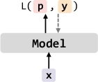
(a) Model Training

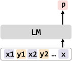
(b) In-context learning

Figure 1: In-context learning and model training learn in different ways , where and are forward and backward processes, respectively, and L($\cdot$,$\cdot$) is the loss function.

Examples	Acc
The casting of Raymond J. Barry as the ‘assassin’ greatly enhances the quality … It was [great]	82.0
At some point , all this visual trickery stops being clever … It was [terrible]	85.3
1. The casting of Raymond … It was [great] 2. At some point , all this visual trickery… It was [terrible]	56.0
1. At some point , all this visual trickery … It was [great] 2. The casting of Raymond … It was [terrible]	74.4

Table 1: The case study of examples’ combinatorial dependency on SST-2, where “it was [great/terrible]” is the template. Although two examples bring good performance separately, combining them instead hurts performance.

There is a similar problem in traditional gradient-based deep learning like fine-tuning (Devlin et al., 2019), typically called Coreset Selection (Guo et al., 2022), which aims to select a set of representative training examples for the dataset to benefit many downstream scenarios like data-efficient learning (Adadi, 2021), active learning (Ren et al., 2022), neural architecture search (Shim et al., 2021), etc. However, it is challenging for these coreset selection methods to select important in-context examples because there is a significant discrepancy between traditional training and ICL. As shown in Figure 1, the “learning” paradigms of model training and ICL are highly different. Traditional training depends on back-propagation’s gradients to update parameters while ICL occurs in LM’s forward process without gradients and parameter updates. Existing coreset selection methods are always coupled with the training procedure, i.e., they usually depend on gradients or run with the training procedure. For example, Paul et al. (2021) select informative examples by their gradients’ norm. Toneva et al. (2019) evaluate each example’s importance by counting how many times it is forgotten, i.e., the example is misclassified after being correctly classified in the previous epoch. Additionally, coreset selection methods mainly depend on the example’s gradients as the feature of example selection (Mirzasoleiman et al., 2020; Killamsetty et al., 2021a, b; Guo et al., 2022). However, LM performs ICL through inference, which does not rely on gradients or parameter updates. Hence, the gap between gradient-based training and ICL makes these methods struggle to effectively select informative examples for in-context learning.

Another challenge is the strong dependency among in-context examples. Previous work (Lu et al., 2022) shows that even the same example set with different orderings can result in drastically different performance from random-guess level to state-of-the-art. Here we also conduct an additional case study to shed light on examples’ combinatorial dependency in Table 1. We see that compared with two examples’ individual performance, combining them instead significantly hurts the performance. To cope with examples’ dependency, a straightforward method is to enumerate all possible examples’ combinations and verify their performance. However, it will lead to combinatorial explosion and thus is infeasible.

To tackle these challenges, we propose LENS, a fiLter-thEN-Search that finds support examples in two stages: in the first stage, we filter the dataset to obtain informative in-context examples individually. Specifically, we propose InfoScore to evaluate the example’s in-context informativeness based on the LM’s feedback, and further propose a progressive filtering process to filter out uninformative examples; In the second stage, we propose a diversity-guided example search method that iteratively refines and evaluates the selected examples to find support examples that can fully depict the task. We summarize our contributions as follows:

• To the best of our knowledge, we are the first to define the support examples selection problem for in-context learning and introduce a novel filter-then-search method to tackle it.

• We conduct experiments on various text classification datasets and compare our method with a wide range of baselines. Experimental results demonstrate that our method significantly outperforms baselines and previous coreset selection methods bring marginal improvements over the random baseline, which shows the necessity of ICL-specific designing for finding support examples.

• We conduct further analyses on support examples and find that they exhibit different trends from random examples in many aspects, which can shed light on the principle of them and ICL. We provide the following key takeaways: 1. Support examples are less sensitive to the order compared with random examples (Lu et al., 2022). 2. Ground truth labels matter for support examples, while the previous study (Min et al., 2022b) show that they are not important for randomly sampled examples. 3. One LM’s support examples can be well transferred to other LMs with different sizes and pre-training corpora and keep the superiority over random examples.

• We provide comprehensive empirical results of previous coreset selection methods on ICL, which has not been explored. We will release the implementation of our method and baselines to facilitate future research.

2 Background:In-Context Learning

In this section, we introduce the definition of in-context learning. We focus on text classification’s in-context learning using the causal language model (Radford et al., 2018). Given a language model $G$, $n$ examples $\{x_{i},y_{i}\}_{i=1}^{n}$ and a test input $x_{test}$, the prediction of $x_{test}$ is generated as:

$$\operatorname*{arg\,max}_{y\in\mathcal{Y}}p_{G}(y|x_{1}\oplus y_{1}\cdots x_{n}\oplus y_{n}\oplus x_{test}),$$ (1)

where $\mathcal{Y}$ is the label space and $\oplus$ is the concatenation operation. To deal with classification tasks, the original label is often mapped to word or words in $G$’s vocabulary. For example, the positive/negative label in a binary sentiment classification can be mapped to “great”/“terrible”. For simplicity, we omit the verbalizer, special tokens and prompting templates in Eq (1).

As Eq.(1) shows, $G$ receives the task’s supervision only from the concatenated $\{x_{i},y_{i}\}_{i=1}^{n}$ and directly output the prediction of $x_{test}$. Typically, $n$ is limited by the max input length of $G$, so it is typical for researchers to randomly sample a small set of samples from the entire dataset $\mathcal{D}$  (Brown et al., 2020; Zhang et al., 2022a). However, ICL is sensitive to the provided examples and random in-context examples show significant instability and probably cause inferior performance(Lu et al., 2022; Chen et al., 2022). In this paper, we focus on selecting a small list of support examples that are informative for the task and performant for in-context learning, from the entire dataset $\mathcal{D}$.

3 Method

The strong dependency among in-context examples makes selecting support examples essentially an NP-hard combinatorial optimization problem. Enumerating all combinations and evaluating them is infeasible due to the combinatorial explosion. In this section, we propose LENS, a fiLter-thEN-Search method to find support examples: 1. we first filter the training dataset to obtain informative examples individually, 2. then we search the example permutation that fully depicts the task from them. In this paper, we instantiate the two stages as a novel example metric with progressive filtering and diversity-guided example search, we leave the development of more powerful components as future work. We introduce these two stages below.

3.1 Informative Examples Filtering

0:  Training set $\mathcal{D}=\{e_{i}\}_{i=1}^{n}$, language model $G$, desired candidate size $m$, progressive factor $\mathcal{\rho}$, initial score data size $l$.

0:  Individually informative examples $\mathcal{D}^{\prime}$

1:  $\mathcal{D^{\prime}}\leftarrow\mathcal{D}$

2:  $S\leftarrow$ Randomly sample $l$ examples from $\mathcal{D}$.

3:  while $|\mathcal{D}^{\prime}|>m$ do

4:     for $e_{i}\sim\mathcal{D}^{\prime}$ do

5:        $\operatorname{s}(e_{i})\leftarrow I(e_{i},S)$

6:     end for

7:     if $|\mathcal{D}^{\prime}|/\mathcal{\rho}<m$ then

8:        $\mathcal{D}^{\prime}\leftarrow$ the top-$m$ of $\mathcal{D}^{\prime}$ using $\{s(e_{i})\}_{i=1}^{|\mathcal{D}^{\prime}|}$

9:        Break;

10:     else

11:        $\mathcal{D}^{\prime}\leftarrow$ the top $\frac{1}{\mathcal{\rho}}$ of $\mathcal{D}^{\prime}$ using $\{s(e_{i})\}_{i=1}^{|\mathcal{D}^{\prime}|}$

12:     end if

13:     $S^{\prime}\leftarrow$ Randomly sample $l*(\mathcal{\rho}-1)$ examples from $\mathcal{D}$

14:     $S\leftarrow S\cup S^{\prime}$

15:  end while

16:  return  $\mathcal{D}^{\prime}$

Algorithm 1 Progressive Example Filtering

In the first stage, we aim to find those informative examples individually. There are extensive methods to measure the example’s importance for gradient-based training, like the example’s gradient norm (Paul et al., 2021), loss value in the early training stage or the times of being forgotten (Toneva et al., 2019), etc. However, these methods struggle to identify important in-context examples since ICL is based on LM-inference without gradients and parameter updates. Here we propose  InfoScore (Informativeness Score) to measure the individual in-context informativeness of one example $e=\{x,y\}$ for ICL based on LM’s feedback as:

$$I(e,\mathcal{D}) =\sum_{e^{\prime}\in\mathcal{D}}c(e,e^{\prime})$$ (2)

$$c(e,e^{\prime}) =p_{G}(y^{\prime}|x,y,x^{\prime})-p_{G}(y^{\prime}|x^{\prime}),$$ (3)

where $e^{\prime}=\{x^{\prime},y^{\prime}\}$, and $\mathcal{D}$ is the training dataset. Eq (3) is the gap between the probabilities of the ground truth $y^{\prime}$ conditioned on $(e,x^{\prime})$ and $(x^{\prime})$, respectively. So it evaluates how informative $e$ is for the LM to correctly classify $x^{\prime}$ and thus measures $e$’s contribution for $e^{\prime}$ in ICL. Hence, $I(e,\mathcal{D})$, the sum of Eq (3) over $\mathcal{D}$, can evaluate the example’s task-level in-context informativeness.

However, computing all examples’ InfoScores over the entire dataset is quadratic in $|\mathcal{D}|$ and thus infeasible. We further propose a progressive filtering process to filter out uninformative examples progressively, where promising examples receive more computation while low-quality examples get less computation, shown in Algorithm 1.

We filter out uninformative examples in a progressive manner. We first sample a small set of examples from $\mathcal{D}$ as initial “score set” (line 2) to coarsely evaluate the InfoScore of each example and filter the entire dataset to 1/$\rho$ of its original size (line 5). At the following iteration, we proportionally expand the size of the score set to $\mathcal{\rho}$ times by randomly sampling more examples from training set (line 13$\sim$15) and use it to calculate InfoScore of the remaining promising examples. As the score set is expanded, the subsequent InfoScore can be calculated in a more fine-grained way and better filter informative examples. Meanwhile, the uninformative examples are filtered out in the previous iteration, which helps save the computational cost. We repeat this procedure until a small set of examples is left.

Thus we achieve filtering examples with high in-context informativeness in the complexity of $O(N*\log_{\mathcal{\rho}}N)$, where $N$ is the size of training set. In experiments, we set $\rho$ to $N^{\frac{1}{C}}$ to make it a linear complexity, where $C$ is a constant. According to the size of dataset, $\rho$ is usually set between 2 - 3.

3.2 Diversity-Guided Example Search

0:  Candidate examples $\mathcal{D}^{\prime}=\{e_{i}\}_{i=1}^{m}$, candidates’ feature $\{f(e_{i})\}_{i=1}^{m}$, a small validation set $V$, iteration num $\mathcal{I}$, beam size $\mathcal{B}$, example substitution size $\mathcal{B}^{\prime}$

0:  A performant examples’ permutation.

1:  $\mathcal{E}=\{E_{i}\}_{i=1}^{\mathcal{B}}\leftarrow$ initialize $\mathcal{B}$ examples’ permutations

2:  for $i$ in $1,2\cdots\mathcal{I}$ do

3:     $\mathcal{E}^{\prime}\leftarrow\{\}$

4:     for $E$ in $\{E_{j}\}_{j=1}^{\mathcal{B}}$ do

5:        for $b$ in $1,2\cdots\mathcal{B}^{\prime}$ do

6:           $e*\leftarrow$Randomly sample an example from $E$

7:           $e^{*}_{new}\leftarrow\operatorname{argmax}_{e\in\mathcal{D}^{\prime}}s(e,E-e^{*})$

8:           $E^{*}\leftarrow$ Replace $e^{*}$ in $E$ with $e^{*}_{new}$

9:           $\mathcal{E}^{\prime}\leftarrow\mathcal{E}^{\prime}\cup\{E^{*}\}$

10:        end for

11:        for $b$ in $1,\cdots\mathcal{B}-\mathcal{B}^{\prime}$ do

12:           $E^{*}\leftarrow$ Randomly shuffle $E$

13:           $\mathcal{E}^{\prime}\leftarrow\mathcal{E}^{\prime}\cup\{E^{*}\}$

14:        end for

15:        $\mathcal{E}\leftarrow$ Evaluate $\mathcal{E}^{\prime}$ on $V$ and get the top-$\mathcal{B}$

16:     end for

17:  end for

18:  return  The top-1 of $\mathcal{E}$

Algorithm 2 Diversity-Guided Search

After filtering, we get individually informative examples $\mathcal{D}^{\prime}$. Since the in-context examples have high combinatorial dependency (see Table 1), a straightforward method is to enumerate all possible combinations and evaluate them on a validataion set. However, although we have reduced the candidate examples by filtering, it is still impossible to evaluate all combinations. For example, if there are 50 examples retained after filtering and we want to find a combination of 8 examples from them, it can lead to $\textbf{C}_{50}^{8}$ (about 536 million) combinations, let alone considering the examples’ orders.

Hence we propose diversity-guided example search to iteratively refine the example selection from filtered examples and obtain the support examples, as shown in Algorithm 2. It starts with a set of initial example permutations. At each iteration, we use the diversity of in-context examples to guide the update of the current candidate permutations. Specifically, for each candidate permutation $E=[e_{i}]_{i=1}^{n}$, we randomly select an example $e^{*}$ in $E$ and update it with the example $e^{*}_{new}$ as:

$$e^{*}_{new} =\operatorname{argmax}_{e\in\mathcal{D}^{\prime}}s(e,E^{\prime})$$ (4)

$$s(e,E^{\prime}) =I(e,S)-\lambda\sum_{e^{\prime}\in E^{\prime}}\operatorname{sim}(f(e),f(e^{\prime})),$$ (5)

where $E^{\prime}=E-e^{*}$, $\lambda$ is pre-defined hyper-parameter, $S=\{e_{i}^{s}\}_{i=1}^{m}$ is the final score set of the filtering stage. The subsequent term of $s(e,E^{\prime})$ in Eq (5) corresponds to the diversity between $e$ and $E^{\prime}$, and $f(\cdot)$ is the example’s feature vector calculated as:

$$f(e)=[c(e,e^{s}_{1}),c(e,e^{s}_{2})\cdots,c(e,e^{s}_{|S|})],$$ (6)

where $f(e)$ describes $e$’s contribution on $S$’s each example $e^{s}_{i}$ in ICL and thus directly encodes $e$’s in-context feature. If two examples’ $f(\cdot)$ are similar, their effect on ICL can be redundant and we should avoid selecting both of them in one permutation. Note that $I(e,S)$ and each $c(e,e^{s}_{i})$ in $f(e)$ are calculated in the filtering stage and can be reused.

With $s(e,E^{\prime})$ and $f(e)$, the updated candidate permutations can be informative and diverse, and help the LM correctly predict various examples, which can better help find the support examples that fully depict the task in ICL. In this paper, we propose and verify a simple yet effective example ICL feature. We leave the development of more powerful ones as future work.

Since examples’ order can significantly influence the performance (Lu et al., 2022), we also update $E$ with different orders by randomly shuffling (line 10$\sim$13), which can reduce the risk of missing performant combinations of examples due to poor ordering. In order To explore the example search space more comprehensively and alleviate risk of the local-optimal example permutation, we consider the beam search (Jurafsky and Martin, 2009) here instead of greedy search. Specifically, we update each candidate example permutations by diversity-based example substitution and random shuffling for $B^{\prime}$ and $B-B^{\prime}$ times, respectively (line 5, 10). Then we leverage a small validation set sampled from $(\mathcal{D}-\mathcal{D}^{\prime})$ to evaluate them and keep the top-$\mathcal{B}$ permutations with best performance as next iteration’s candidates. Through these, we can the mitigate issue of local-optimal example permutation, better iteratively refine and evaluate the candidate permutations with high informativeness and diversity in turn and obtain the examples that can fully depict the task.

To initialize example permutations $E$ with informativeness and diversity, we formulate it as discrete optimization that maximizes $\sum_{e\in E}s(e,E-e)$, which can be solved by the discrete optimization solver like CPLEX (Cplex, 2009).

4 Experiments

4.1 Experimental Settings

Dataset

In this paper, we conduct experiments on eight text classification datasets across three task families, including Sentiment Classification: SST-2, SST-5 (Socher et al., 2013), Amazon (McAuley and Leskovec, 2013) and MR (Pang and Lee, 2005); Subjectivity Classification: Subj (Pang and Lee, 2004); Topic Classification: TREC (Voorhees and Tice, 2000), AGNews (Zhang et al., 2015) and DBPedia (Lehmann et al., 2015).

Method Comparison

We mainly compare our proposed methods with the following baselines: Random: We randomly select examples from the training set; Random & Validation: We evaluate multiple sets of random examples on the validation set and select the best one. We consider Random & Validation under two settings whose computational cost is similar to our method: 1. the size of validation set is the same as ours at stage 2 (100) and the number of random example sets is the same as our searched and evaluated example permutations (640). 2. the size of validation set is larger, 1000, and the number of random example sets is 100. We also consider a wide range of Coreset Selection methods in gradient-based learning scenarios, according to the methodologies, they can be divided into multiple categories including: Geometry-Based Method: it assumes that data points that are close in the feature space have similar properties, including Herding (Chen et al., 2012) and K-Center Greedy (Sener and Savarese, 2018); Uncertainty-Based Method: it assumes examples with higher uncertainty can have a greater impact on the model and should be contained in coreset, including Least Confidence, Entropy, Margin (Coleman et al., 2020) and CAL (Margatina et al., 2021); Error/Loss Based Method: It assumes the example that contributes more to the error or loss during training is more important and should be included in coreset, including Forgetting (Toneva et al., 2019) and GraNd (Paul et al., 2021); Gradient Matching Based Method: Since deep models are usually trained by gradient descent, it tries to find a coreset whose gradients can imitate the entire dataset’s gradients, including CRAIG (Mirzasoleiman et al., 2020) and GradMatch (Killamsetty et al., 2021a); Submodularity-Based Method: Submodular functions (Iyer and Bilmes, 2013) naturally measure a subset’s informativeness and diversity and can thus be powerful for coreset selection, including Facility Location and Graph Cut (Iyer and Bilmes, 2013); Bilevel Optimization Based Method: It transforms the coreset selection problem into a bilevel-optimization problem whose outer and inner objectives are subset selection and model parameter optimization, respectively: Glister (Killamsetty et al., 2021b). Due to the page limit, we introduce these methods and their implementation details in Appendix A and Appendix B.1, respectively.

Implementation Details

For the LM, we follow  Min et al. (2022a) to use GPT2-L (Radford et al., 2018). We set the number of retained examples of filtering $m$, the weight of diversity $\lambda$, the beam size $\mathcal{B}$ and the number of diversity search iterations as 500, 1, 8 and 10 respectively. We show the overall hyper-parameters, implementation details, analysis details and complexity analysis in Appendix B. For baselines and LENS, we run each method under 4 prompt templates over 10 random seeds (40 in total) and report the average performance with and without calibration (Zhao et al., 2021), unless otherwise specified. We show the overall templates and dataset statistics in Appendix C and D.

4.2 Main Results

Method	SST-2	SST-5	Amazon	MR	Subj	TREC	AGNews	DBPedia	Average
zero-shot	63.0/80.3	27.5/33.3	31.2/37.6	61.7/77.4	51.0/52.0	38.7/27.7	59.8/59.9	32.3/37.6	45.6/50.7
Random	57.9/64.4	27.5/23.9	73.7/78.5	59.5/67.1	55.0/60.9	30.3/24.9	33.6/47.8	16.3/64.7	44.2/54.0
Herding	62.0/63.7	24.8/20.5	75.4/71.9	54.1/57.3	56.5/56.7	26.4/22.2	38.7/35.7	7.4/61.7	43.2/48.7
K-Center Greedy	58.6/61.6	25.1/23.0	78.6/76.3	59.0/61.3	59.9/57.0	31.3/26.4	42.3/37.8	32.1/72.1	48.4/51.9
Entropy	62.4/67.4	25.5/26.6	71.4/76.2	54.1/56.2	53.9/51.7	26.2/21.3	30.6/35.3	14.5/46.9	42.3/47.7
LeastConfidence	58.4/63.0	26.0/23.2	73.8/72.1	55.9/57.3	58.0/51.9	23.5/21.5	31.6/36.7	9.1.59.9	42.0/48.2
Margin	62.4/67.4	26.1/22.6	76.9/76.6	54.1/56.2	53.9/51.7	24.2/21.0	38.1/45.0	7.1/58.4	42.9/49.9
Cal	59.3/66.7	25.3/25.5	75.7/75.4	66.2/67.7	64.6/55.6	31.8/30.7	42.3/46.6	30.3/73.9	49.4/55.3
Forgetting	61.6/68.2	27.7/23.5	77.1/78.2	56.7/59.4	55.1/53.2	28.7/28.6	33.4/39.8	10.5/64.7	43.9/52.0
GraNd	54.6/56.5	27.8/24.9	75.5/73.4	52.8/55.8	55.7/51.9	28.2/23.9	33.4/53.2	21.2/64.0	43.7/50.5
CRAIG	63.4/72.0	26.4/25.3	75.4/80.6	59.3/66.7	57.0/54.8	32.0/24.8	37.4/55.4	29.5/71.0	47.6/56.3
GradMatch	57.0/61.9	26.3/23.4	75.1/76.0	56.6/62.1	55.8/64.6	25.8/21.4	32.6/39.4	9.7/57.8	42.3/49.6
FacilityLocation	65.5/73.2	23.9/24.3	77.7/77.6	61.7/69.6	59.0/54.5	35.7/29.1	42.5/58.6	30.4/74.3	49.6/57.7
GraphCut	65.0/71.4	25.3/24.6	76.5/78.4	66.3/72.3	63.2/56.6	34.7/28.4	41.9/50.8	14.0/47.3	48.4/53.7
Glister	59.0/61.0	25.8/25.2	78.0/77.7	60.1/66.6	60.6/57.0	29.4/23.4	38.6/41.1	24.1/69.8	46.7/52.7
Random & Valid (100)	70.1/72.8	33.2/29.6	76.3/78.4	53.2/57.9	60.7/58.9	30.3/24.9	40.1/33.6	37.2/56.7	50.1/51.6
Random & Valid (1000)	65.0/62.6	29.0/30.8	78.5/78.6	57.7/62.5	61.9/53.4	32.8/29.4	43.5/56.1	37.8/73.6	49.5/55.9
LENS	86.3/87.6	44.9/42.1	80.2/83.9	83.1/83.9	86.4/81.5	59.0/48.8	77.9/78.1	40.8/80.7	69.8/73.3

Table 2: Results on GPT2-L. Each entry shows the ICL accuracy without and with calibration (Zhao et al., 2021).

We show the results in Table 2. We observe that our method significantly outperforms baselines on all datasets with or without calibration mechanism, which shows our method’s best overall ability to find task-representative support examples across different settings and task families. Specially, our method shows better performance than the Random-Validation baseline and this directly demonstrates its non-triviality. Meanwhile, previous methods for gradient-based learning have similar performance with the Random baseline, and this indicates: 1. there is a non-negligible gap between ICL and these methods 2. it is necessary to design to ICL-specific method to find support examples.

Additionally, the Random baseline slightly underperforms the Zero-Shot, which shows that random examples are hard to fully characterize the task and the necessity of finding support examples for ICL. In experiments, we observe that Random-Validation suffers from the ICL’s instability. Specifically, we find that considerable example permutations selected by the validation set do not consistently yield satisfactory results on the test set and this degrades its performance, whereas our method is more robust and less susceptible to this issue.

4.3 Analysis

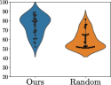
(a) SST-2

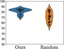
(b) Amazon

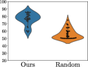
(c) MR

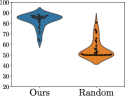
(d) Subj

Figure 2: The performance distribution of support examples and random examples with multiple orders.

The Sensitivity of Support Examples to Orders

The recent study (Lu et al., 2022) shows that the ordering of in-context examples for ICL has a significant influence on the performance. Specifically, to the same set of randomly sampled examples, different orders can result in near state-of-the-art and random-guess performance. In this section, we explore the effect of ordering for our support examples on SST-2, Amazon, MR and Subj. For each task, we select four sets of support examples and four sets of random examples and then evaluate their performance with eight randomly sampled orders. We show the performance distribution in Figure 2. We see that random examples with different orders show highly unstable performance where the worst drops to the random-guess level, which is consistent with the conclusion in previous work (Lu et al., 2022). In contrast, the support examples’ performance is significantly more stable than random examples. Generally, most orders can still lead to approximately equivalent performance as the searched orders and few orders lead to the random-guess performance. The phenomenon is compatible with the conclusion from the recent work (Chen et al., 2022), which shows a strong negative correlation between ICL sensitivity and accuracy. Moreover, our support examples’ lower sensitivity to the ordering demonstrates that they can more effectively depict and characterize the corresponding task.

Examples	SST-2	MR	TREC	AGNews	Average
GPT2-XL
Random	60.3	66.7	34.4	56.9	54.6
LENS	73.0	70.7	44.0	60.4	62.0
GPT2-M
Random	59.6	65.0	33.4	51.7	52.4
LENS	82.0	75.5	37.5	75.3	67.6
GPT-Neo-2.7B
Random	57.3	55.8	29.4	71.6	53.5
LENS	62.5	65.2	45.0	80.2	63.2

Table 3: The transfer of GPT2-L’s support examples on LMs with different sizes and pre-training corpora: GPT2-M, GPT2-XL and GPT-Neo-2.7B.

Transferablity across Different LMs

In the main experiments, we get GPT2-L’s support examples and evaluate them using the same LM. And here we explore the transferability of these support examples across different LMs with various sizes and pre-training corpora. Specifically, we test the support examples of main experiments on GPT2-M (355M), GPT2-XL (1.5B) and GPT-Neo-2.7B (Black et al., 2021). The results are shown in Table 3. We see that GPT2-L’s support examples also show better performance than the Random baseline. Additionally, our support examples also demonstrate the consistent superiority on GPT-Neo-2.7B which has a different pre-training corpus from GPT2-L. Since random examples’ performance can not be well transferred to other LMs (Lu et al., 2022), these can show the strong transferability of our support examples and the utility of our method when more powerful LMs are proposed.

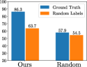
(a) SST-2

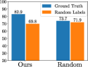
(b) Amazon

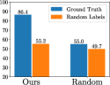
(c) Subj

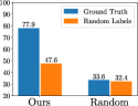
(d) AGNews

Figure 3: The results under gold and random labels.

Ground Truth Matters for Support Examples

Recently, Min et al. (2022b) suggests that ground truth (GT) labels are not important for ICL, which differs from traditional supervised learning. In their experiments, for randomly sampled examples, using ground truth labels or not leads to similar ICL performance. Here we explore the effect of ground truth labels for support examples. We show the performance of support examples and random examples with GT or random labels in Figure 3. We see that the results on random examples are consistent with that in the previous paper (Min et al., 2022b). However, we observe a significantly different trend in support examples. Specifically, after removing GT labels, support examples’ performance gets a strong degradation. We suppose it is because while random examples can not characterize the task well and thus their GT labels are not important, the GT labels of support examples contain crucial task information and input-output correspondence, so their GT labels are important for ICL’s performance. Meanwhile, we find that under random labels, support examples also yield noticeable improvements over the random examples, which indicates that the inputs of support examples are also more informative for the task.

The Impact of Hyper-parameters

	SST-2	Subj	TREC	Average
Random	57.9	55.0	30.3	47.7
$p$=1.5	86.6	86.1	59.5	77.4
$p$=2	86.3	86.4	59.0	77.2
$p$=3	85.1	86.0	58.7	76.6
$m$ = 50	83.6	84.1	56.2	74.6
$m$ = 500	86.3	86.4	59.0	77.2
$m$ = 1000	86.1	85.9	59.1	77.0
$\lambda$ = 1	86.3	86.4	59.3	77.3
$\lambda$ = 2	86.5	86.2	58.8	77.2
$\lambda$ = 0.5	85.9	86.1	58.7	76.9
$\lambda$ = 0	67.5	68.2	37.7	57.8
$\mathcal{B}$ = 1	83.1	76.2	42.2	67.2
$\mathcal{B}$ = 4	85.9	86.0	58.5	76.8
$\mathcal{B}$ = 8	86.3	86.4	59.0	77.2

Table 4: Impact of different hyper-parameters.

In this section, we evaluate the effect of each hyper-parameter. Specifically, we evaluate the effect of progressive ratio $p$, the number of stage 1’s retained examples $m$, the weight of diversity $\lambda$ and the beam size $\mathcal{B}$ by separately tuning them and observing performance. Table 4 shows the results. When $\mathcal{B}$ is set to 0, i.e., we remove stage 2 and just select those examples with the highest InfoScore, the performance gets significantly degraded, and this directly demonstrates the effectiveness and necessity of stage 2. Except when $\mathcal{B}=0$, our method leads to consistent performance improvements compared with the Random baseline in general, across various hyper-parameter configurations, which indicates our method’s robustness to hyper-parameters. Meanwhile, we observe two slight performance degradations when $m=100$ or $\mathcal{B}=1$. For the case that $m=100$, we suppose that is because there are too few examples being retained after stage 1, limiting candidate examples’ diversity. When $\mathcal{B}=1$, our stage 2 degrades to greedy search guided by the diversity, causing it susceptible to the local optimum issue.

InfoScore and Progressive Filtering

	Subj	AGNews
Random	55.0	33.6
Filtering (Uninformative)	52.5	27.4
Filtering (Informative)	65.8	47.8
Filtering + Search	86.4	77.9

Table 5: The Effect of Progressive Filtering.

In this section, we evaluate the effect of InfoScore and progressive filtering in stage 1. Specifically, we randomly sample examples from the retained examples of stage 1 and test their average performance across 4 prompt templates with 10 random orders (40 in total). We compare the Random baseline, our filtering method and another filtering variant that filters uninformative examples, which retains those examples with low InfoScore at each iteration. We show the results in Table 5. We observe that just the proposed filtering method also leads to better ICL performance than randomly sampled examples, which directly shows that stage 1 is effective for filtering out the uninformative examples. Meanwhile, the performance points of Filtering (Informative), Random and Filtering (Uninformative) present a descending trend, which demonstrates that the proposed InfoScore can indicate the examples’ in-context informativeness. However, compared with our entire method, Filtering (Informative) still shows a significant discrepancy. This indicates the necessity of considering in-context examples’ dependency and the effectiveness of the proposed diversity-guided search.

5 Related Work

Since we introduce a wide range of coreset selection methods in Section 4.1, we omit them here and mainly introduce previous works about example selection for ICL. Previous works mainly consider example-level retrieval for ICL. Liu et al. (2022) leverage a semantic embedder to retrieve relevant examples for the given test input. Das et al. (2021) and Hu et al. (2022) use dense retrievers trained by task-specific targets’ similarities to retrieve in-context examples for question answering and dialogue state tracking, respectively. Rubin et al. (2022); Shi et al. (2022) train the demonstration retriever based on the feedback of the language model for semantic parsing. Wu et al. (2022) use Sentence-BERT (Reimers and Gurevych, 2019) to retrieve relevant examples and introduce an information-theoretic-driven criterion to rerank their permutations. Levy et al. (2022); Ye et al. (2023) further consider diversity in example retrieval. Different from these methods which aim to provide example-specific information for the test input, we focus on task-level example selection, which seeks to find examples that are representative for the task and is complementary to them. Moreover, because the large language models (Brown et al., 2020; Zhang et al., 2022a; Black et al., 2021) almost adopt purely causal Transformer (Vaswani et al., 2017) decoder architecture, we can calculate task-level in-context examples representation in advance and reuse them for different test inputs. Since these two settings’ goals are orthogonal and complementary, we regard the hybrid setting and method as future work. Another line of methods is active learning (Ren et al., 2022) for ICL. It aims to select some examples from a large pool of unlabeled data and annotate them for ICL. Zhang et al. (2022b) propose to learn an active example selector by off-line reinforcement learning and use it to select examples to annotate for ICL. Su et al. (2022) propose a graph-based annotation method, vote-k, and use Sentence-BERT to retrieve relevant examples from the annotated examples for ICL. In this paper, we explore a different setting for ICL’s example selection, where we select support examples from the annotated dataset since there are massive annotated datasets for various tasks and the prevailing large language model has shown impressive data annotation ability (Efrat and Levy, 2020; Gao et al., 2022; Ye et al., 2022; Meng et al., 2022).

6 Conclusion

In this paper, we propose a two-stage filter-then-search method to find support examples for in-context learning from the annotated dataset: First we propose InfoScore to select informative examples individually with a progressive filtering process. Then we propose diversity-guided example search which iteratively refines and evaluates the selected examples, to find the example permutations that fully depict the task. The experimental results show that our method significantly outperforms extensive baselines, and further analyses show that each component contributes critically to the improvements and shed light on the principles of support examples and in-context learning.

Limitations

These are the limitations of this work:

• Due to the computation resources limitation, we mainly conduct experiments on GPT2-L (Radford et al., 2018) and analyze the cross-LM transferability of support examples in section 4.3. We see the exploration on more LMs as future work.

• In this paper, the proposed filter-then-search framework explores how to find support examples of in-context learning. We see exploring and analyzing more principles of in-context learning as future work.

• Language models have exhibited various kinds of bias (Bender et al., 2021), since our filtering stage is based on its feedback, the filtered example might also exhibit these biases. We see language model debiasing as an important future research topic.

Appendix A Baselines

We mainly compare our proposed methods with following baselines: Random: We randomly select examples with random orderings from the training set; Random & Validation: We evaluate multiple sets of random examples on the validation set and select the best one. We consider Random & Validation under two settings whose computational cost is similar to our method: 1. the size of validation set is the same as ours at stage 2 (100) and the number of random example sets is the same as our searched and evaluated example permutations (640). 2. the size of validation set is larger, 1000, and the number of random example sets is 100. We also consider a wide range of Coreset Selection methods in traditional gradient-based learning scenarios, according to the methodologies, they can be divided into multiple categories including: Geometry-Based Method: it assumes that data points that are close in the feature space have similar properties. The Herding method (Chen et al., 2012) adds one data point each time into the coreset to greedily minimize the distance between coreset center and the original dataset center. The K-Center Greedy method (Sener and Savarese, 2018) selects examples to minimize the largest distance between each example in coreset and its closest example in set of examples that are not in coreset. Uncertainty-Based Method: it assumes examples with higher uncertainty can have a greater impact on the model and should be contained in coreset. Coleman et al. (2020) propose Least Confidence (the max probability over all labels), Entropy and Margin (max probability margin between different labels) to measure the examples’ uncertainty scores and build coreset. CAL (Margatina et al., 2021) selects examples whose predictive likelihood exhibits the greatest divergence from their neighbors to build the coreset. Error/Loss Based Method: It assumes the example that contributes more to the error or loss during training is more important and should be added to coreset. Toneva et al. (2019) propose Forgetting to evaluate each example’s importance by counting how many times it is forgotten, i.e., it is misclassified after begin correctly classified in previous training epochs. Paul et al. (2021) propose the GraNd score to select informative examples. GraNd is the gradient norm expectation of the example. The larger one example’s GraNd is, the more important it is. Gradient Matching Based Method: Since deep models are usually trained by gradient descent, it tries to find a coreset whose gradients can imitate the entire dataset’s gradients. Mirzasoleiman et al. (2020) propose CRAIG to convert the gradient matching problem to the maximization of a monotone submodular function and optimize it greedily. Killamsetty et al. (2021a) propose GradMatch based on CRAIG, which adds a regularization term to discourage assigning large weights to individual examples and improves the used greedy algorithm. Submodularity-Based Method: Submodular functions (Iyer and Bilmes, 2013) naturally measure the subset’s informativeness and diversity and thus can be powerful for coreset selection. Iyer and Bilmes (2013) leverage Facility Location and Graph Cut as submodular functions to select the coreset. Bilevel Optimization Based Method: It transforms the coreset selection problem into a bilevel-optimization problem whose outer and inner objectives are subset selection and model parameter optimization, respectively. Glister (Killamsetty et al., 2021b) leverages a validation set on the outer optimization and the log-likelihood in the bilevel optimization.

To reduce the gap between these methods and ICL, we use the same LM (GPT2-L) with “last pooling” fine-tuned on the whole dataset for 5 epochs to obtain relevant metrics, e.g., gradients or forgetting times for these methods. Following Guo et al. (2022), we use the gradients of the final fully-connected layer’s parameters as these methods’ example feature.

Appendix B Implementation Details

B.1 Baseline Details

For those previous coreset selection methods, to reduce the gap between these methods and ICL, we use the same LM (GPT2-L) with “last pooling” fine-tuned on the whole dataset for 5 epochs to obtain relevant metrics, e.g., gradients or forgetting times for these methods. Following Guo et al. (2022), we use the gradients of the final fully-connected layer’s parameters as these methods’ example feature. For baselines that output a weighted subset of examples, e.g., CRAIG or GradMatch, we just adopt its examples for simplicity since there are few methods to weighting in-context examples for ICL.

B.2 Method Details

We find each prompting template’s corresponding support examples separately in our method and compared methods, i.e., we select examples for each prompting template separately. For simplicity, we calculate Eq (3) without calibration for experiments without or with calibration. For the filtering stage, we set the progressive factor and the size of initial score set according to the dataset’s size. Specifically, we set the progressive factor to make the filter iterations be 4.

We run all experiments under the label balance setting and the total number of in-context examples for most datasets except DBPedia is set to 8. The number of some datasets’ in-context examples is not 8 but close to 8 because 8 can not be divided by the number of its labels, e.g., 5 for SST-5. Since DBPedia has 14 labels and significantly longer input sequence, we run experiments on it under the label-unbalance setting and set the total number of examples to 4. In label balance setting, we 1. filter the same number of examples for each label, 2. initialize the example permutation of stage 2 with balanced labels 3. update $e^{*}$ with $e^{*}_{new}$, whose label is the same as $e^{*}$.

We list the total number of examples in Table 6. And we set the size of initial score set to make the times of LM’s forwards to be around 10K. We list the progressive factor $p$ and the size of initial score set $|S_{0}|$in Table 7. For other hyper-parameters, we conduct grid search for the number of retained examples of filtering $m$, the weight of diversity $\lambda$, the beam size $\mathcal{B}$ and the iteration of diversity-guided search over {500,1000}, {0.5,1,2}, {4,8,16} and {5,10,15} respectively on the SST-2 dataset. And we set them to be 500, 1, 8 and 10 respectively.

B.3 Experimental Details

In section “The Sensitivity of Support Examples to Orders”, since the performance is sensitive to the prompting templates, we show the performance distribution under a specific prompting template. In other analysis experiments, for simplicity, we report the average performance under four different prompting templates without calibration, unless otherwise specified.

B.3.1 The Complexity of Our Method

Progressive Filtering

in the filtering stage, we need to compute pairwise Eq 3 for $N*l*\rho/\rho=N*l$ times, where $N$ is size of training set. Since we filter the dataset into $1/\rho$ of its previous size until a small set of examples is left, the number of iteration is $log_{\mathcal{\rho}}N)$. Thus the filtering stage’s complexity over $N$ is $O(N*\log_{\mathcal{\rho}}N)$. In experiments, we set $\rho$ to $N^{\frac{1}{C}}$ to make it a linear complexity, where $C$ is a constant. According to the size of dataset, $\rho$ is usually set between 2 - 3, shown in Table 7.

Diversity-Guided Example Search

At each iteration, we have $\mathcal{B}$ candidate permutations and separately update them $B$ times. And then we evaluate these updated candidate permutations on the small validation set sampled from the remaining training set, whose size is fixed. Since updating the candidate permutations reuses the intermediate results of the filtering stage and does not involve the computation of the LLM (see Eq (4) and (5)), we omit it for complexity analysis. So the complexity of diversity-guided example search is consistant, $\mathcal{B}*\mathcal{B}$.

Appendix C Prompting Templates

We show the prompting verbalizers and templates in Table 8.

Appendix D Dataset Split and Statistics

We use the same dataset split in the previous work (Min et al., 2022a). Due to computational resource limitations, for Amazon, AGNews and DBPedia, we conduct experiments on a randomly sampled subset of it (30000 and 2000 for the training and test set), and we show the overall dataset statistics in Table 6.

	Training Size	Test Size	Label	Examples
SST-2	6921	873	2	8
SST-5	8544	2210	5	10
Amazon	30000	2000	2	8
MR	8662	2000	2	8
Subj	8000	2000	2	8
TREC	5452	500	6	12
AGNews	30000	7601	4	8
DBPedia	30000	2000	14	4

Table 6: Data statistics.

	$p$	$|S_{0}|$
SST-2	2	14
SST-5	2	11
Amazon	3	4
MR	2	11
Subj	2	12
TREC	2	20
AGNews	3	4
DBPedia	3	4

Table 7: The progressive factor $p$ and the size of initial score set $S_{0}$ for each dataset.

0.95p0.92

Task Family: Sentiment Classification

Task: SST-2

Prompting Verbalizer: {great, terrible}

Prompting Templates:

• “[INPUT] A [VERBALIZER] one. ”

• “[INPUT] It was [VERBALIZER]. ”

• “[INPUT] All in all [VERBALIZER]. ”

• “[INPUT] A [VERBALIZER] piece. ”

Example:

Input:
I have to admit that I am baffled by jason x.

It was terrible.
If you answered yes, by all means enjoy the new guy.

It was great.
$\cdots$

Never comes together as a coherent whole.

It was

Output:

terrible.

Task: SST-5

Prompting Verbalizer: {great, good, okay, bad, terrible}

Prompting Templates: Same as SST-2

Task: Amazon

Prompting Verbalizer: {great, good, okay, bad, terrible}

Prompting Templates: Same as SST-2

Task: MR

Prompting Verbalizer: {great, terrible}

Prompting Templates: Same as SST-2

Task Family: Topic Classification

Task: TREC

Prompting Verbalizer: {Description, Entity, Expression, Human, Location, Number}

Prompting Templates:

• “[INPUT] Topic: [VERBALIZER]. ”

• “[INPUT] Subject: [VERBALIZER]. ”

• “[INPUT] This is about [VERBALIZER]. ”

• “[INPUT] It is about [VERBALIZER] piece. ”

Example:

Input:
How do storms form ?

Topic: Description.
What city in Florida is Sea World in?

Topic: Location.
$\cdots$

What university fired Angela Davis?

Topic:

Output:

Human.

Task: AGNews

Prompting Verbalizer: {World, Sports, Business, Technology}

Prompting Templates: Same as TREC

Task: DBPedia

Prompting Verbalizer: {Company, Educational Institution, Artist, Athlete, Office Holder, Mean of Transportation, Building, Natural Place, Village, Animal, Plant, Album, Film, Written Work}

Prompting Templates: Same as AGNews

Task Family: Subjective Classification

Task: Subj

Prompting Verbalizer: {subjective, objective}

Prompting Templates:

• “[INPUT] This is [VERBALIZER]. ”

• “[INPUT] It’s all [VERBALIZER]. ”

• “[INPUT] It’s [VERBALIZER]. ”

• “[INPUT] Is it [VERBALIZER]? ”

Example:

Input:
There are two distince paths in life good vs . evil. It’s subjective.
Photographed with melancholy richness and eloquently performed yet also decidedly uncinematic.

It’s objective.
$\cdots$

The film is an homage to power , strength and individualism.

It’s

Output:

subjective

Table 8: The prompting verbalizers and templates for each task.

References

- Adadi (2021) Amina Adadi. 2021. A survey on data-efficient algorithms in big data era. J. Big Data, 8(1):1–54.
- Bender et al. (2021) Emily M. Bender, Timnit Gebru, Angelina McMillan-Major, and Shmargaret Shmitchell. 2021. On the dangers of stochastic parrots: Can language models be too big? In FAccT ’21: 2021 ACM Conference on Fairness, Accountability, and Transparency, Virtual Event / Toronto, Canada, March 3-10, 2021, pages 610–623. ACM.
- Black et al. (2021) Sid Black, Leo Gao, Phil Wang, Connor Leahy, and Stella Biderman. 2021. GPT-Neo: Large Scale Autoregressive Language Modeling with Mesh-Tensorflow.
- Brown et al. (2020) Tom B. Brown, Benjamin Mann, Nick Ryder, Melanie Subbiah, Jared Kaplan, Prafulla Dhariwal, Arvind Neelakantan, Pranav Shyam, Girish Sastry, Amanda Askell, Sandhini Agarwal, Ariel Herbert-Voss, Gretchen Krueger, Tom Henighan, Rewon Child, Aditya Ramesh, Daniel M. Ziegler, Jeffrey Wu, Clemens Winter, Christopher Hesse, Mark Chen, Eric Sigler, Mateusz Litwin, Scott Gray, Benjamin Chess, Jack Clark, Christopher Berner, Sam McCandlish, Alec Radford, Ilya Sutskever, and Dario Amodei. 2020. Language models are few-shot learners. In Advances in Neural Information Processing Systems 33: Annual Conference on Neural Information Processing Systems 2020, NeurIPS 2020, December 6-12, 2020, virtual.
- Chang and Jia (2023) Ting-Yun Chang and Robin Jia. 2023. Data curation alone can stabilize in-context learning.
- Chen et al. (2022) Yanda Chen, Chen Zhao, Zhou Yu, Kathleen R. McKeown, and He He. 2022. On the relation between sensitivity and accuracy in in-context learning. CoRR, abs/2209.07661.
- Chen et al. (2012) Yutian Chen, Max Welling, and Alexander J. Smola. 2012. Super-samples from kernel herding. CoRR, abs/1203.3472.
- Coleman et al. (2020) Cody Coleman, Christopher Yeh, Stephen Mussmann, Baharan Mirzasoleiman, Peter Bailis, Percy Liang, Jure Leskovec, and Matei Zaharia. 2020. Selection via proxy: Efficient data selection for deep learning. In 8th International Conference on Learning Representations, ICLR 2020, Addis Ababa, Ethiopia, April 26-30, 2020. OpenReview.net.
- Cortes and Vapnik (1995) Corinna Cortes and Vladimir Vapnik. 1995. Support-vector networks. Machine learning, 20(3):273–297.
- Cplex (2009) IBM ILOG Cplex. 2009. V12. 1: User’s manual for cplex. International Business Machines Corporation, 46(53):157.
- Das et al. (2021) Rajarshi Das, Manzil Zaheer, Dung Thai, Ameya Godbole, Ethan Perez, Jay Yoon Lee, Lizhen Tan, Lazaros Polymenakos, and Andrew McCallum. 2021. Case-based reasoning for natural language queries over knowledge bases. In Proceedings of the 2021 Conference on Empirical Methods in Natural Language Processing, EMNLP 2021, Virtual Event / Punta Cana, Dominican Republic, 7-11 November, 2021, pages 9594–9611. Association for Computational Linguistics.
- Devlin et al. (2019) Jacob Devlin, Ming-Wei Chang, Kenton Lee, and Kristina Toutanova. 2019. BERT: pre-training of deep bidirectional transformers for language understanding. In Proceedings of the 2019 Conference of the North American Chapter of the Association for Computational Linguistics: Human Language Technologies, NAACL-HLT 2019, Minneapolis, MN, USA, June 2-7, 2019, Volume 1 (Long and Short Papers), pages 4171–4186. Association for Computational Linguistics.
- Dong et al. (2022) Qingxiu Dong, Lei Li, Damai Dai, Ce Zheng, Zhiyong Wu, Baobao Chang, Xu Sun, Jingjing Xu, Lei Li, and Zhifang Sui. 2022. A survey for in-context learning.
- Efrat and Levy (2020) Avia Efrat and Omer Levy. 2020. The turking test: Can language models understand instructions? CoRR, abs/2010.11982.
- Gao et al. (2022) Jiahui Gao, Renjie Pi, Yong Lin, Hang Xu, Jiacheng Ye, Zhiyong Wu, Xiaodan Liang, Zhenguo Li, and Lingpeng Kong. 2022. Zerogen: Self-guided high-quality data generation in efficient zero-shot learning. CoRR, abs/2205.12679.
- Guo et al. (2022) Chengcheng Guo, Bo Zhao, and Yanbing Bai. 2022. Deepcore: A comprehensive library for coreset selection in deep learning. In Database and Expert Systems Applications - 33rd International Conference, DEXA 2022, Vienna, Austria, August 22-24, 2022, Proceedings, Part I, volume 13426 of Lecture Notes in Computer Science, pages 181–195. Springer.
- Hu et al. (2022) Yushi Hu, Chia-Hsuan Lee, Tianbao Xie, Tao Yu, Noah A. Smith, and Mari Ostendorf. 2022. In-context learning for few-shot dialogue state tracking. CoRR, abs/2203.08568.
- Iyer and Bilmes (2013) Rishabh K. Iyer and Jeff A. Bilmes. 2013. Submodular optimization with submodular cover and submodular knapsack constraints. In Advances in Neural Information Processing Systems 26: 27th Annual Conference on Neural Information Processing Systems 2013. Proceedings of a meeting held December 5-8, 2013, Lake Tahoe, Nevada, United States, pages 2436–2444.
- Jurafsky and Martin (2009) Dan Jurafsky and James H. Martin. 2009. Speech and language processing: an introduction to natural language processing, computational linguistics, and speech recognition, 2nd Edition. Prentice Hall series in artificial intelligence. Prentice Hall, Pearson Education International.
- Killamsetty et al. (2021a) KrishnaTeja Killamsetty, Durga Sivasubramanian, Ganesh Ramakrishnan, Abir De, and Rishabh K. Iyer. 2021a. GRAD-MATCH: gradient matching based data subset selection for efficient deep model training. In Proceedings of the 38th International Conference on Machine Learning, ICML 2021, 18-24 July 2021, Virtual Event, volume 139 of Proceedings of Machine Learning Research, pages 5464–5474. PMLR.
- Killamsetty et al. (2021b) KrishnaTeja Killamsetty, Durga Sivasubramanian, Ganesh Ramakrishnan, and Rishabh K. Iyer. 2021b. GLISTER: generalization based data subset selection for efficient and robust learning. In Thirty-Fifth AAAI Conference on Artificial Intelligence, AAAI 2021, Thirty-Third Conference on Innovative Applications of Artificial Intelligence, IAAI 2021, The Eleventh Symposium on Educational Advances in Artificial Intelligence, EAAI 2021, Virtual Event, February 2-9, 2021, pages 8110–8118. AAAI Press.
- Lehmann et al. (2015) Jens Lehmann, Robert Isele, Max Jakob, Anja Jentzsch, Dimitris Kontokostas, Pablo N. Mendes, Sebastian Hellmann, Mohamed Morsey, Patrick van Kleef, Sören Auer, and Christian Bizer. 2015. Dbpedia - A large-scale, multilingual knowledge base extracted from wikipedia. Semantic Web, 6(2):167–195.
- Levy et al. (2022) Itay Levy, Ben Bogin, and Jonathan Berant. 2022. Diverse demonstrations improve in-context compositional generalization. CoRR, abs/2212.06800.
- Liu et al. (2022) Jiachang Liu, Dinghan Shen, Yizhe Zhang, Bill Dolan, Lawrence Carin, and Weizhu Chen. 2022. What makes good in-context examples for gpt-3? In Proceedings of Deep Learning Inside Out: The 3rd Workshop on Knowledge Extraction and Integration for Deep Learning Architectures, DeeLIO@ACL 2022, Dublin, Ireland and Online, May 27, 2022, pages 100–114. Association for Computational Linguistics.
- Lu et al. (2022) Yao Lu, Max Bartolo, Alastair Moore, Sebastian Riedel, and Pontus Stenetorp. 2022. Fantastically ordered prompts and where to find them: Overcoming few-shot prompt order sensitivity. In Proceedings of the 60th Annual Meeting of the Association for Computational Linguistics (Volume 1: Long Papers), pages 8086–8098, Dublin, Ireland. Association for Computational Linguistics.
- Margatina et al. (2021) Katerina Margatina, Giorgos Vernikos, Loïc Barrault, and Nikolaos Aletras. 2021. Active learning by acquiring contrastive examples. In Proceedings of the 2021 Conference on Empirical Methods in Natural Language Processing, EMNLP 2021, Virtual Event / Punta Cana, Dominican Republic, 7-11 November, 2021, pages 650–663. Association for Computational Linguistics.
- McAuley and Leskovec (2013) Julian J. McAuley and Jure Leskovec. 2013. Hidden factors and hidden topics: understanding rating dimensions with review text. In Seventh ACM Conference on Recommender Systems, RecSys ’13, Hong Kong, China, October 12-16, 2013, pages 165–172. ACM.
- Meng et al. (2022) Yu Meng, Martin Michalski, Jiaxin Huang, Yu Zhang, Tarek F. Abdelzaher, and Jiawei Han. 2022. Tuning language models as training data generators for augmentation-enhanced few-shot learning. CoRR, abs/2211.03044.
- Min et al. (2022a) Sewon Min, Mike Lewis, Hannaneh Hajishirzi, and Luke Zettlemoyer. 2022a. Noisy channel language model prompting for few-shot text classification. In Proceedings of the 60th Annual Meeting of the Association for Computational Linguistics (Volume 1: Long Papers), ACL 2022, Dublin, Ireland, May 22-27, 2022, pages 5316–5330. Association for Computational Linguistics.
- Min et al. (2022b) Sewon Min, Xinxi Lyu, Ari Holtzman, Mikel Artetxe, Mike Lewis, Hannaneh Hajishirzi, and Luke Zettlemoyer. 2022b. Rethinking the role of demonstrations: What makes in-context learning work? In Proceedings of the 2022 Conference on Empirical Methods in Natural Language Processing, EMNLP 2022, Abu Dhabi, United Arab Emirates, December 7-11, 2022, pages 11048–11064. Association for Computational Linguistics.
- Mirzasoleiman et al. (2020) Baharan Mirzasoleiman, Jeff A. Bilmes, and Jure Leskovec. 2020. Coresets for data-efficient training of machine learning models. In Proceedings of the 37th International Conference on Machine Learning, ICML 2020, 13-18 July 2020, Virtual Event, volume 119 of Proceedings of Machine Learning Research, pages 6950–6960. PMLR.
- Pang and Lee (2004) Bo Pang and Lillian Lee. 2004. A sentimental education: Sentiment analysis using subjectivity summarization based on minimum cuts. In Proceedings of the 42nd Annual Meeting of the Association for Computational Linguistics, 21-26 July, 2004, Barcelona, Spain, pages 271–278. ACL.
- Pang and Lee (2005) Bo Pang and Lillian Lee. 2005. Seeing stars: Exploiting class relationships for sentiment categorization with respect to rating scales. In ACL 2005, 43rd Annual Meeting of the Association for Computational Linguistics, Proceedings of the Conference, 25-30 June 2005, University of Michigan, USA, pages 115–124. The Association for Computer Linguistics.
- Paul et al. (2021) Mansheej Paul, Surya Ganguli, and Gintare Karolina Dziugaite. 2021. Deep learning on a data diet: Finding important examples early in training. In Advances in Neural Information Processing Systems 34: Annual Conference on Neural Information Processing Systems 2021, NeurIPS 2021, December 6-14, 2021, virtual, pages 20596–20607.
- Radford et al. (2018) Alec Radford, Jeffrey Wu, Rewon Child, David Luan, Dario Amodei, and Ilya Sutskever. 2018. Language models are unsupervised multitask learners.
- Reimers and Gurevych (2019) Nils Reimers and Iryna Gurevych. 2019. Sentence-bert: Sentence embeddings using siamese bert-networks. In Proceedings of the 2019 Conference on Empirical Methods in Natural Language Processing and the 9th International Joint Conference on Natural Language Processing, EMNLP-IJCNLP 2019, Hong Kong, China, November 3-7, 2019, pages 3980–3990. Association for Computational Linguistics.
- Ren et al. (2022) Pengzhen Ren, Yun Xiao, Xiaojun Chang, Po-Yao Huang, Zhihui Li, Brij B. Gupta, Xiaojiang Chen, and Xin Wang. 2022. A survey of deep active learning. ACM Comput. Surv., 54(9):180:1–180:40.
- Rubin et al. (2022) Ohad Rubin, Jonathan Herzig, and Jonathan Berant. 2022. Learning to retrieve prompts for in-context learning. In Proceedings of the 2022 Conference of the North American Chapter of the Association for Computational Linguistics: Human Language Technologies, NAACL 2022, Seattle, WA, United States, July 10-15, 2022, pages 2655–2671. Association for Computational Linguistics.
- Sener and Savarese (2018) Ozan Sener and Silvio Savarese. 2018. Active learning for convolutional neural networks: A core-set approach. In 6th International Conference on Learning Representations, ICLR 2018, Vancouver, BC, Canada, April 30 - May 3, 2018, Conference Track Proceedings. OpenReview.net.
- Shi et al. (2022) Peng Shi, Rui Zhang, He Bai, and Jimmy Lin. 2022. XRICL: cross-lingual retrieval-augmented in-context learning for cross-lingual text-to-sql semantic parsing. CoRR, abs/2210.13693.
- Shim et al. (2021) Jae-hun Shim, Kyeongbo Kong, and Suk-Ju Kang. 2021. Core-set sampling for efficient neural architecture search. CoRR, abs/2107.06869.
- Socher et al. (2013) Richard Socher, Alex Perelygin, Jean Wu, Jason Chuang, Christopher D. Manning, Andrew Y. Ng, and Christopher Potts. 2013. Recursive deep models for semantic compositionality over a sentiment treebank. In Proceedings of the 2013 Conference on Empirical Methods in Natural Language Processing, EMNLP 2013, 18-21 October 2013, Grand Hyatt Seattle, Seattle, Washington, USA, A meeting of SIGDAT, a Special Interest Group of the ACL, pages 1631–1642. ACL.
- Su et al. (2022) Hongjin Su, Jungo Kasai, Chen Henry Wu, Weijia Shi, Tianlu Wang, Jiayi Xin, Rui Zhang, Mari Ostendorf, Luke Zettlemoyer, Noah A. Smith, and Tao Yu. 2022. Selective annotation makes language models better few-shot learners. CoRR, abs/2209.01975.
- Toneva et al. (2019) Mariya Toneva, Alessandro Sordoni, Remi Tachet des Combes, Adam Trischler, Yoshua Bengio, and Geoffrey J. Gordon. 2019. An empirical study of example forgetting during deep neural network learning. In 7th International Conference on Learning Representations, ICLR 2019, New Orleans, LA, USA, May 6-9, 2019. OpenReview.net.
- Vaswani et al. (2017) Ashish Vaswani, Noam Shazeer, Niki Parmar, Jakob Uszkoreit, Llion Jones, Aidan N. Gomez, Lukasz Kaiser, and Illia Polosukhin. 2017. Attention is all you need. In Advances in Neural Information Processing Systems 30: Annual Conference on Neural Information Processing Systems 2017, December 4-9, 2017, Long Beach, CA, USA, pages 5998–6008.
- Voorhees and Tice (2000) Ellen M. Voorhees and Dawn M. Tice. 2000. Building a question answering test collection. In SIGIR 2000: Proceedings of the 23rd Annual International ACM SIGIR Conference on Research and Development in Information Retrieval, July 24-28, 2000, Athens, Greece, pages 200–207. ACM.
- Wu et al. (2022) Zhiyong Wu, Yaoxiang Wang, Jiacheng Ye, and Lingpeng Kong. 2022. Self-adaptive in-context learning. CoRR, abs/2212.10375.
- Ye et al. (2022) Jiacheng Ye, Jiahui Gao, Zhiyong Wu, Jiangtao Feng, Tao Yu, and Lingpeng Kong. 2022. Progen: Progressive zero-shot dataset generation via in-context feedback. In Findings of the Association for Computational Linguistics: EMNLP 2022, Abu Dhabi, United Arab Emirates, December 7-11, 2022, pages 3671–3683. Association for Computational Linguistics.
- Ye et al. (2023) Jiacheng Ye, Zhiyong Wu, Jiangtao Feng, Tao Yu, and Lingpeng Kong. 2023. Compositional exemplars for in-context learning. CoRR, abs/2302.05698.
- Zhang et al. (2022a) Susan Zhang, Stephen Roller, Naman Goyal, Mikel Artetxe, Moya Chen, Shuohui Chen, Christopher Dewan, Mona T. Diab, Xian Li, Xi Victoria Lin, Todor Mihaylov, Myle Ott, Sam Shleifer, Kurt Shuster, Daniel Simig, Punit Singh Koura, Anjali Sridhar, Tianlu Wang, and Luke Zettlemoyer. 2022a. OPT: open pre-trained transformer language models. CoRR, abs/2205.01068.
- Zhang et al. (2015) Xiang Zhang, Junbo Jake Zhao, and Yann LeCun. 2015. Character-level convolutional networks for text classification. In Advances in Neural Information Processing Systems 28: Annual Conference on Neural Information Processing Systems 2015, December 7-12, 2015, Montreal, Quebec, Canada, pages 649–657.
- Zhang et al. (2022b) Yiming Zhang, Shi Feng, and Chenhao Tan. 2022b. Active example selection for in-context learning. CoRR, abs/2211.04486.
- Zhao et al. (2023) Wayne Xin Zhao, Kun Zhou, Junyi Li, Tianyi Tang, Xiaolei Wang, Yupeng Hou, Yingqian Min, Beichen Zhang, Junjie Zhang, Zican Dong, Yifan Du, Chen Yang, Yushuo Chen, Zhipeng Chen, Jinhao Jiang, Ruiyang Ren, Yifan Li, Xinyu Tang, Zikang Liu, Peiyu Liu, Jian-Yun Nie, and Ji-Rong Wen. 2023. A survey of large language models. CoRR, abs/2303.18223.
- Zhao et al. (2021) Zihao Zhao, Eric Wallace, Shi Feng, Dan Klein, and Sameer Singh. 2021. Calibrate before use: Improving few-shot performance of language models. In Proceedings of the 38th International Conference on Machine Learning, ICML 2021, 18-24 July 2021, Virtual Event, volume 139 of Proceedings of Machine Learning Research, pages 12697–12706. PMLR.