Natural Gradient Hybrid Variational Inference with Application to Deep Mixed Models

Weiben Zhang is a PhD student and Michael Smith is Professor of Management (Econometrics) at the Melbourne Business School, University of Melbourne, Australia. Worapree Maneesoonthorn is Associate Professor and Rubén Loaiza-Maya is Senior Lecturer at the Department of Econometrics and Business Statistics, Monash University, Australia. Worapree Maneesoonthorn gratefully acknowledges support by the Australian Research Council through grant DP200101414. Rubén Loaiza-Maya gratefully acknowledges support by the Australian Research Council through grant DE230100029. Weiben Zhang gratefully acknowledges support from the University of Melbourne through the Faculty of Business and Economics Graduate Research Scholarship. Correspondence should be directed to Michael Smith at mikes70au@gmail.com.

Stochastic models with global parameters $\theta$ and latent variables $z$ are common, and variational inference (VI) is popular for their estimation. This paper uses a variational approximation (VA) that comprises a Gaussian with factor covariance matrix for the marginal of $\theta$, and the exact conditional posterior of $\text{\boldmath$z$}|\text{\boldmath$\theta$}$. Stochastic optimization for learning the VA only requires generation of $z$ from its conditional posterior, while $\theta$ is updated using the natural gradient, producing a hybrid VI method. We show that this is a well-defined natural gradient optimization algorithm for the joint posterior of $(\text{\boldmath$z$},\text{\boldmath$\theta$})$. Fast to compute expressions for the Tikhonov damped Fisher information matrix required to compute a stable natural gradient update are derived. We use the approach to estimate probabilistic Bayesian neural networks with random output layer coefficients to allow for heterogeneity. Simulations show that using the natural gradient is more efficient than using the ordinary gradient, and that the approach is faster and more accurate than two leading benchmark natural gradient VI methods. In a financial application we show that accounting for industry level heterogeneity using the deep model improves the accuracy of probabilistic prediction of asset pricing models.

Keywords: Asset Pricing; Bayesian Neural Networks; Natural Gradient Optimization; Random Coefficients; Re-parameterization trick; Tikhonov damping; Variational Bayes.

1 Introduction

Black box variational inference (VI) methods (Ranganath et al.,, 2014) that employ a generic approximating family for the Bayesian posterior distribution are popular. The approximation is usually learned by minimizing the Kullback-Leibler divergence between the two, with stochastic gradient ascent (SGA) the most common choice of algorithm to solve the optimization problem (Bottou,, 2010, Hoffman et al.,, 2013). Here, the variational approximation (VA) is updated in the direction of the (noisy) ordinary gradient of the objective function. However, the natural gradient gives the steepest direction for this optimization problem (Amari,, 1998), and stochastic natural gradient ascent (SNGA) is an alternative algorithm that can converge in fewer steps and avoid plateaus in the objective function (Rattray et al.,, 1998, Martens,, 2020). But for large scale problems computing the natural gradient is usually impractical for approximations outside the exponential family. In this paper, we show that the natural gradient can be computed quickly for the VA family proposed by Loaiza-Maya et al., (2022), thereby extending the class of VAs to which SNGA can be applied. Doing so can greatly reduce the time required to learn this approximation compared to SGA.

Loaiza-Maya et al., (2022) suggested a VI method where the target vector $\psi$ is partitioned into two components $\text{\boldmath$\psi$}=(\text{\boldmath$\theta$}^{\top},\text{\boldmath$z$}^{\top})^{\top}$. The method samples $z$ from its conditional posterior, while using (noisy) ordinary gradients to update the marginal VA for $\theta$. The authors show these two steps together form a well-defined SGA algorithm for solving the variational optimization for the joint posterior of $\psi$, and call their method “hybrid VI”. The approach is particularly useful when $z$ is a high-dimensional vector of latent variables, which are also sometimes called local parameters (Hoffman et al.,, 2013). However, the method can suffer from slow convergence in common with other first order stochastic optimization methods for a number of problems, such as training some neural networks (Zhang et al.,, 2018). In this paper we improve the efficiency of hybrid VI by using SNGA optimization. The objective is to reduce the number of draws of $z$—typically the slowest step of the algorithm—by providing faster convergence of the variational optimization. We show that the combination of natural gradient based optimization and hybrid VI provides a particularly attractive VI method for complex high-dimensional target posteriors.

The natural gradient is equal to the ordinary gradient pre-multiplied by the inverse of the Fisher information matrix (FIM) (Amari,, 1998), and the computation, storage and factorization of the latter can be costly. We show that in hybrid VI the FIM of the VA of $\psi$ is equal to that of the FIM of the marginal VA of $\theta$. When the dimension of $\theta$ is low relative to that of $z$—as is often the case when $z$ is a vector of latent variables—then the additional cost of computing the natural gradient of the VA for $\psi$ is minor compared to the ordinary gradient. This additional cost is more than off-set by the savings gained from the smaller number of draws of $z$ required, thus improving the overall efficiency of the hybrid VI algorithm. For the marginal VA of $\theta$ we use a Gaussian distribution with a factor covariance matrix (Miller et al.,, 2017, Mishkin et al.,, 2018, Ong et al., 2018a, , Tran et al.,, 2020). Fast to compute analytical re-parameterized natural gradient updates that use the Tikhonov damped Fisher information matrix are derived. Tikhonov damping, combined with adaptive learning rates, addresses the numerical difficulties often encountered with natural gradient updates when training complex models (Osawa et al.,, 2019).

There is growing interest in using NGA in VI. Martens, (2020) gives an overview and discussion of NGA as a second order optimization method, while Martens and Grosse, (2015), Khan and Nielsen, (2018) and Zhang et al., 2019b show that natural gradient based VI methods can improve the efficiency of training neural networks, which we also find here. Khan and Nielsen, (2018) consider the case where the VA is from the exponential family, and Lin et al., (2019) where the VA is a mixture of exponential distributions. Martens and Grosse, (2015) and Tran et al., (2020) approximate the FIM by block diagonal matrices to reduce computation cost. Tan, (2022) considers efficient application of SNGA to learn high-dimensional Gaussian VAs based on Cholesky factorization, whereas Lin et al., (2021) suggests transforming the variational parameters to simplify computation of the natural gradient for some fixed form VAs.

We illustrate our VI approach by using it to estimate several stochastic models. Our main focus is on deep mixed models (DMM), which are a class of probabilistic Bayesian neural networks. Mixed models (also called random coefficient or multi-level models) are widely used to capture heterogeneity in statistical modeling (McCulloch and Searle,, 2004), and DMMs extend this approach to deep learning  (Wikle,, 2019, Tran et al.,, 2020, Simchoni and Rosset,, 2021). Following Tran et al., (2020), in our DMM the output layer coefficients vary by a group variable and follow a Gaussian distribution, allowing for heterogeneity. To apply hybrid VI, the vector $z$ contains the output layer group level coefficient values. Using simulation studies, we establish that SNGA is much faster and more reliable than SGA for learning the VA in hybrid VI. We also show for our examples that the natural gradient hybrid VI is faster and more accurate than the alternative natural gradient based VI methods of Tran et al., (2020) and Tan, (2022).

Recent studies suggests that deep models have strong potential in financial modeling (Gu et al.,, 2020, 2021, Fang and Taylor,, 2021). We use our approach to estimate three factor (Fama and French,, 1993) and five factor (Fama and French,, 2015) financial asset pricing models. We use monthly returns on 2583 stocks between January 2005 and December 2014 to train a DMM with feed forward neural network architecture that accounts for heterogeneity in 548 industry groups. Accuracy of the learned model is assessed using posterior predictive distributions computed for both the training data, and also for a validation period from January 2015 to December 2019. The results suggest that the DMM improves probabilistic predictive accuracy compared to existing (non-deep) linear mixed modeling, and (non-mixed) feed forward neural networks.

The rest of the paper is organized as follows. Section 2 provides a brief introduction to the hybrid VI approach, and Section 3 extends hybrid VI to employ the natural gradient. Section 4 outlines DMMs and in simulation studies shows how natural gradient hybrid VI leads to an increase in computational efficiency and accuracy for training a DMM, compared to both ordinary gradient hybrid VI and the benchmark natural gradient methods of Tran et al., (2020) and Tan, (2022). Section 5 contains the financial asset pricing study, while Section 6 discusses the contribution of our study and directions for future work.

2 Hybrid Variational Inference

2.1 Variational inference

We consider a stochastic model with data $y$ and unknowns $\psi$. Bayesian inference for $\psi$ employs its posterior density $p(\text{\boldmath$\psi$}|\text{\boldmath$y$})\propto p(\text{\boldmath$y$}|\text{\boldmath$\psi$})p(\text{\boldmath$\psi$})\equiv g(\text{\boldmath$\psi$})$, where $p(\text{\boldmath$y$}|\text{\boldmath$\psi$})$ is the likelihood and $p(\text{\boldmath$\psi$})$ is the prior. The posterior is often difficult to evaluate, and in VI it is approximated using a density $q(\text{\boldmath$\psi$})\in{\cal Q}$, with ${\cal Q}$ a family of flexible but tractable densities. The density $q$ is called the “variational approximation” (VA) and obtained by minimizing a distance metric between $p(\text{\boldmath$\psi$}|\text{\boldmath$y$})$ and $q(\text{\boldmath$\psi$})$. The Kullback-Leibler divergence (KLD) is the most popular choice, and it is easily shown that minimizing the KLD corresponds to maximizing the Evidence Lower Bound (ELBO)

$$\mathcal{L}=E_{q}\left[\log g(\text{\boldmath$\psi$})-\log q(\text{\boldmath$\psi$})\right]$$

over $q\in{\cal Q}$, where the expectation above is with respect to $\text{\boldmath$\psi$}\sim q$. This optimization problem is called “variational optimization” and the method used for its solution determines the speed of the VI method; for overviews of VI see Ormerod and Wand, (2010), Blei et al., (2017), and Zhang et al., 2019a .

2.2 Variational inference for latent variable models

Stochastic models that have both unknown parameters $\theta$ and latent variables $z$ are popular. Examples include mixed models where $z$ are random coefficients (Tran et al.,, 2020), tobit models where $z$ are uncensored data (Danaher et al.,, 2020), state space models where $z$ are latent states (Wang et al.,, 2022), and topic models where $z$ are topics (Blei et al.,, 2003). There are a number of ways to apply VI to this case. The most popular strategy is to set $\text{\boldmath$\psi$}=(\text{\boldmath$\theta$}^{\top},\text{\boldmath$z$}^{\top})^{\top}$ and approximate the “augmented posterior” $p(\text{\boldmath$\psi$}|\text{\boldmath$y$})$; for recent examples, see Hoffman and Blei, (2015), Loaiza-Maya and Smith, (2019) and Tan, (2021). However, because $\mbox{dim}(\text{\boldmath$z$})$ is often very large, approximating the augmented posterior can introduce substantial cumulative error. One alternative is to integrate out $z$ using numerical or Monte Carlo methods, such as importance sampling (Gunawan et al.,, 2017, Tran et al.,, 2020). However, this can prove slow or even computationally infeasible for large models. Another alternative that is both accurate and scalable was suggested by Loaiza-Maya et al., (2022), which we briefly outline below.

2.3 Hybrid variational inference

For latent variable models consider the VA

$$q_{\lambda}(\text{\boldmath$\psi$})=p(\text{\boldmath$z$}|\text{\boldmath$\theta$},\text{\boldmath$y$})q^{0}_{\lambda}(\text{\boldmath$\theta$})\,,$$ (1)

where $q^{0}_{\lambda}(\text{\boldmath$\theta$})$ is the density of a fixed form VA with parameters $\lambda$. Then it is possible to show that the ELBO for the augmented posterior of $\text{\boldmath$\psi$}=(\text{\boldmath$\theta$}^{\top},\text{\boldmath$z$}^{\top})^{\top}$ is equal to the ELBO of the marginal posterior of $\theta$; that is,

$${\cal L}(\text{\boldmath$\lambda$})\equiv E_{q_{\lambda}}\left[\log g(\text{\boldmath$\psi$})-\log q_{\lambda}(\text{\boldmath$\psi$})\right]=E_{q^{0}_{\lambda}}\left[\log\left(p(\text{\boldmath$y$}|\text{\boldmath$\theta$})p(\text{\boldmath$\theta$})\right)-\log q^{0}_{\lambda}(\text{\boldmath$\theta$})\right]\equiv{\cal L}^{0}(\text{\boldmath$\lambda$})\,.$$ (2)

Here, both ELBO’s are denoted as functions of $\lambda$ because this vector parameterizes both $q^{0}_{\lambda}$ and $q_{\lambda}\in{\cal Q}$. The equality at (2) means that solving the variational optimization for $\psi$ with respect to $\lambda$ also solves the variational optimization problem for $\theta$ with $z$ integrated out exactly. We stress this point because it is the source of the increased accuracy of this VI method.

Loaiza-Maya et al., (2022) use a stochastic gradient ascent (SGA) algorithm (Bottou,, 2010) to solve the variational optimization. The key input to SGA is an unbiased estimate of the ordinary gradient $\nabla_{\lambda}{\cal L}(\text{\boldmath$\lambda$})$ , and these authors show how the re-parameterization trick (Kingma and Welling,, 2014, Rezende et al.,, 2014) combined with the VA at (1) gives an efficient gradient estimate. The re-parameterization is of the model parameters $\text{\boldmath$\theta$}=h(\text{\boldmath$\varepsilon$}^{0},\text{\boldmath$\lambda$})\sim q^{0}_{\lambda}$ in terms of a random vector $\text{\boldmath$\varepsilon$}^{0}\sim f_{\text{\boldmath$\varepsilon$}^{0}}$ that is invariant to $\lambda$, and a deterministic function $h$. The latent variables $z$ are not re-parameterized. If the joint density of $\text{\boldmath$\varepsilon$}=\left((\text{\boldmath$\varepsilon$}^{0})^{\top},\text{\boldmath$z$}^{\top}\right)^{\top}$ is denoted as

$$f_{\text{\boldmath$\varepsilon$}}(\text{\boldmath$\varepsilon$})=f_{\text{\boldmath$\varepsilon$}}(\text{\boldmath$\varepsilon$}^{0},\text{\boldmath$z$})=f_{\text{\boldmath$\varepsilon$}^{0}}(\text{\boldmath$\varepsilon$}^{0})p(\text{\boldmath$z$}|h(\text{\boldmath$\varepsilon$}^{0},\text{\boldmath$\lambda$}),\text{\boldmath$y$})\,,$$

then Loaiza-Maya et al., (2022) show that the gradient can be written as an expectation with respect to $\text{\boldmath$\varepsilon$}\sim f_{\varepsilon}$ as

$$\nabla_{\lambda}\mathcal{L}(\bm{\lambda})=E_{f_{\varepsilon}}\left[\frac{\partial h(\text{\boldmath$\varepsilon$},\text{\boldmath$\lambda$})^{\top}}{\partial\text{\boldmath$\lambda$}}\left(\nabla_{\theta}\log g(\text{\boldmath$\theta$},\text{\boldmath$z$})-\nabla_{\theta}\log q_{\lambda}^{0}(\text{\boldmath$\theta$})\right)\right]\,.$$ (3)

An unbiased approximation to the expectation is evaluated by plugging in a single draw from $f_{\varepsilon}$ obtained by first drawing from $f_{\varepsilon^{0}}$, and then from $p(\text{\boldmath$z$}|\text{\boldmath$\theta$},\text{\boldmath$y$})$ with $\text{\boldmath$\theta$}=h(\text{\boldmath$\varepsilon$}^{0},\text{\boldmath$\lambda$})$. For many stochastic models, generation from $p(\text{\boldmath$z$}|\text{\boldmath$\theta$},\text{\boldmath$y$})$ can be done either exactly or approximately using MCMC or other methods. This provides a framework where MCMC can be used within a well-defined SGA variational optimization, so that these authors refer to the method as hybrid VI. In the next section we extend the approach of these authors to use the natural gradient to further reduce the computational burden of hybrid VI.

3 Natural Gradient Hybrid Variational Inference

3.1 Natural gradient ascent

Given a starting value $\text{\boldmath$\lambda$}^{(0)}$, SGA recursively updates the variational parameters as

$$\bm{\lambda}^{(t+1)}=\bm{\lambda}^{(t)}+\bm{\rho}^{(t)}\circ\left.\widehat{\nabla_{\lambda}\mathcal{L}(\bm{\lambda})}\right|_{\text{\boldmath$\lambda$}=\text{\boldmath$\lambda$}^{(t)}},\;t=0,1,\ldots$$ (4)

until reaching convergence. Here, $\bm{\rho}^{(t)}$ are adaptive learning rates, ‘$\circ$’ is the Hadamard (element-wise) product, and $\widehat{\nabla_{\lambda}\mathcal{L}(\bm{\lambda})}$ is an unbiased estimator of the gradient that is evaluated at $\text{\boldmath$\lambda$}=\text{\boldmath$\lambda$}^{(t)}$. While convergence of SGA follows from the conditions in Robbins and Monro, (1951), the algorithm does not exploit the information geometry of $q_{\lambda}(\bm{\psi})$ that can increase the speed of convergence in variational optimization (Khan and Nielsen,, 2018). In contrast, using the natural gradient does so (Amari,, 1998, Honkela et al.,, 2010). The main idea is that $\widehat{\nabla_{\lambda}\mathcal{L}(\bm{\lambda})}$ is replaced in (4) by the unbiased estimate of the natural gradient

$$\widetilde{\nabla}_{\lambda}\mathcal{L}(\bm{\lambda})\equiv F(\bm{\lambda})^{-1}\widehat{\nabla_{\lambda}\mathcal{L}(\bm{\lambda})},$$ (5)

where the Fisher information matrix (FIM)

$$F(\bm{\lambda})=E_{q_{\lambda}}\left[\nabla_{\lambda}\log q_{\lambda}(\bm{\psi})\nabla_{\lambda}\log q_{\lambda}(\bm{\psi})^{\top}\right]=-E_{q_{\lambda}}\left[\frac{\partial^{2}\log q_{\lambda}(\text{\boldmath$\psi$})}{\partial\text{\boldmath$\lambda$}\partial\text{\boldmath$\lambda$}^{\top}}\right]\,,$$

points $\widehat{\nabla_{\lambda}\mathcal{L}(\bm{\lambda})}$ towards the steepest direction of the objective function. This approach, known as stochastic natural gradient ascent (SNGA), typically requires far fewer iterations to reach convergence than SGA; see Martens, (2020) for a recent overview of natural gradient optimization.

The main requirement of NGA is that a tractable expression for $F(\bm{\lambda})$ is available. Its derivation for the VA at (1) may appear challenging, but Theorem 1 shows that $F(\text{\boldmath$\lambda$})$ for this VA is tractable whenever the FIM for $q^{0}_{\lambda}$ is also.

Theorem 1 (Fisher information matrix for hybrid VI).

Let $q_{\lambda}(\text{\boldmath$\psi$})=p(\text{\boldmath$z$}|\text{\boldmath$\theta$},\text{\boldmath$y$})q^{0}_{\text{\boldmath$\lambda$}}(\text{\boldmath$\theta$})$ and denote the Fisher information matrix of the marginal approximation $q^{0}_{\lambda}(\bm{\theta})$ as $F^{0}(\bm{\lambda})=E_{q_{\lambda}^{0}}\left[\nabla_{\lambda}\log q_{\lambda}^{0}(\bm{\theta})\nabla_{\lambda}\log q_{\lambda}^{0}(\bm{\theta})^{\top}\right]$. Then it holds that

$$F(\bm{\lambda})=F^{0}(\bm{\lambda})$$

Proof: See Appendix A

The corollary below follows immediately from Theorem 1.

Corollary 1.1 (Natural gradient for hybrid VI).

If $\widehat{\nabla_{\lambda}\mathcal{L}(\bm{\lambda})}$ is an unbiased estimate of the gradient of the evidence lower bound, then an unbiased estimate of the natural gradient is given by

$$\widetilde{\nabla}_{\lambda}\mathcal{L}(\bm{\lambda})=F^{0}(\bm{\lambda})^{-1}\widehat{\nabla_{\lambda}\mathcal{L}(\bm{\lambda})}\,.$$ (6)

Theorem 1 and Corollary 1.1 have three important implications for the use of SNGA to solve the variational optimization problem with the VA at (1). First, the natural gradient can be constructed for a wide range of latent variable models because it does not require evaluation of the density $p(\text{\boldmath$z$}|\text{\boldmath$\theta$},\text{\boldmath$y$})$ or its derivative, but only the ability to generate from it. Second, evaluation of the natural gradient is scalable with respect to the dimension of $z$. In contrast, other VI methods for latent variables can scale poorly; for example, the computational complexity of the FIM increases with the dimension of $\bm{z}$ for the VA in Tan, (2022). A third implication is that in Corollary 1.1 the computation of the FIM and $\widehat{\nabla_{\lambda}\mathcal{L}(\bm{\lambda})}$ can be done separately. This allows variance reduction techniques when estimating the latter, such as the use of control variates (Paisley et al.,, 2012, Ranganath et al.,, 2014, Tran et al.,, 2017) or the re-parametrization trick as adopted here. Algorithm 1 gives our proposed natural gradient hybrid VI approach, which we label “NG-HVI”. Tikhonov damping is used in step (c) as now discussed.

Initiate $\text{\boldmath$\lambda$}^{(0)}$ and set $t=0$

repeat

     (a) Generate $\text{\boldmath$\theta$}^{(t)}\sim q_{\lambda^{(t)}}^{0}(\text{\boldmath$\theta$})$ using its re-parametrized representation

     (b) Generate ${\text{\boldmath$z$}}^{(t)}\sim p(\text{\boldmath$z$}|{\text{\boldmath$\theta$}}^{(t)},\text{\boldmath$y$})$

     (c) Compute the (Tikhonov damped and stochastic) natural gradient

$$\widetilde{\nabla}_{\lambda}\mathcal{L}(\text{\boldmath$\lambda$}^{(t)})=\widetilde{F}^{0}(\bm{\lambda}^{(t)})^{-1}\left.\widehat{\nabla_{\lambda}\mathcal{L}(\bm{\lambda})}\right|_{\text{\boldmath$\lambda$}=\text{\boldmath$\lambda$}^{(t)}}$$

     (d) Compute step size $\bm{\rho}^{(t)}$ using an adaptive method (e.g. an ADA method)

     (e) Set $\text{\boldmath$\lambda$}^{(t+1)}=\text{\boldmath$\lambda$}^{(t)}+\bm{\rho}^{(t)}\circ\widetilde{\nabla}_{\lambda}\mathcal{L}(\text{\boldmath$\lambda$}^{(t)})$

     (f) Set $t=t+1$

until either a stopping rule is satisfied or a fixed number of steps is taken

Algorithm 1 Hybrid VI with Stochastic Natural Gradient Ascent (NG-HVI)

3.2 Tikhonov damping

The natural gradient can provide an unreliable update in regions where the FIM is close to singular, or where the objective function has high curvature. For example, both problems can arise in training complex deep models (Martens and Grosse,, 2015, Osawa et al.,, 2019). There is an extensive literature on improving the stability of second order optimization, and here we employ Tikhonov damping combined with an adaptive learning rate. We replace $F^{0}$ in (6) with the damped FIM

$$\widetilde{F}^{0}(\bm{\lambda})=F^{0}(\bm{\lambda})+\delta\text{diag}\left(F^{0}(\bm{\lambda})\right)\,,$$ (7)

where $\operatorname{diag}(F^{0})$ is a diagonal matrix comprising the leading diagonal elements of $F^{0}$, and $\delta>0$ is a damping factor. Damping moves the FIM away from singular and unstable values, while taking into account the scale. In our empirical studies we set $\delta=10$, which produces strong results, although performance of the training algorithm may be further improved by tuning $\delta$ as in George et al., (2018) and Osawa et al., (2019). We combine Tikhonov damping with a momentum based adaptive step size from the ADA family—we use ADADELTA of Zeiler, (2012)—which is widely observed to improve convergence for stochastic gradient optimization.

3.3 Fixed form approximation

For the marginal VA of $\theta$, we use Gaussian VAs $q_{\lambda}^{0}(\text{\boldmath$\theta$})=\phi_{m}(\text{\boldmath$\theta$};\text{\boldmath$\mu$},\Sigma)$ with a factor model covariance matrix, also called “low rank plus diagonal”, as suggested by Miller et al., (2017), Ong et al., 2018a and Mishkin et al., (2018). If $m=\mbox{dim}(\text{\boldmath$\theta$})$, then $\Sigma=BB^{\top}+D^{2}$, with $D$ a diagonal matrix and $B$ an $(m\times p)$ matrix where $p<<m$, so that the number of variational parameters scales linearly with $m$. We set the upper triangular elements of $B$ to zero and the leading diagonal elements unconstrained, which can increase the speed of optimization. The variational parameters are $\text{\boldmath$\lambda$}=(\text{\boldmath$\mu$}^{\top},\mbox{vech}(B)^{\top},\text{\boldmath$d$}^{\top})^{\top}$, where “vech” is the half-vectorization operator is applied to a rectangular matrix, and $d$ is a vector containing the non-zero entries of $D$.

An advantage of this factorization is that it has a convenient generative representation given by

$$\text{\boldmath$\theta$}=\text{\boldmath$\mu$}+B\text{\boldmath$\varepsilon$}_{1}^{0}+\text{\boldmath$d$}\circ\text{\boldmath$\varepsilon$}_{2}^{0}\,,$$

that defines the transformation $h$ with $\text{\boldmath$\varepsilon$}^{0}=((\text{\boldmath$\varepsilon$}_{1}^{0})^{\top},(\text{\boldmath$\varepsilon$}_{2}^{0})^{\top})^{\top}\sim N(\bm{0},I_{m+p})$. A second advantage is that the derivatives of $q^{0}_{\lambda}$ required to evaluate the re-parameterized gradient at (3) are given in closed form in Ong et al., 2018a and are fast to compute. A third advantage is that the damped natural gradient $\widetilde{F}^{0}(\bm{\lambda})^{-1}\widehat{\nabla_{\lambda}\mathcal{L}(\bm{\lambda})}$ can also be computed efficiently as follows.

Ong et al., 2018b show that the FIM is sparse with

$$F^{0}(\text{\boldmath$\lambda$})=\left[\begin{array}[]{ccc}F_{11}(\text{\boldmath$\lambda$})&\bm{0}&\bm{0}\\ \bm{0}&F_{22}(\text{\boldmath$\lambda$})&F_{32}(\text{\boldmath$\lambda$})^{\top}\\ \bm{0}&F_{32}(\text{\boldmath$\lambda$})&F_{33}(\text{\boldmath$\lambda$})\\ \end{array}\right]\,,$$ (8)

where the block matrices in $F^{0}$ follow the partition of $\lambda$, and $\bm{0}$ denotes a conformable matrix of zeros. These authors derive closed form expressions for $F_{11},F_{22},F_{32}$ and $F_{33}$. The damped FIM is equal to (8) but with the leading diagonal blocks replaced by $\widetilde{F}_{jj}(\text{\boldmath$\lambda$})=F_{jj}(\text{\boldmath$\lambda$})+\delta\mbox{diag}\left(F_{jj}(\text{\boldmath$\lambda$})\right)$ for $j=1,2,3$. The first elements of the damped natural gradient can be computed as $\widetilde{F}_{11}(\text{\boldmath$\lambda$})^{-1}\widehat{\nabla_{\mu}{\cal L}(\text{\boldmath$\lambda$})}$, using the closed form expression for $\widetilde{F}_{11}(\text{\boldmath$\lambda$})^{-1}$ given in Appendix B. The remaining elements

$$\left[\begin{array}[]{cc}\widetilde{F}_{22}(\text{\boldmath$\lambda$})&F_{32}(\text{\boldmath$\lambda$})^{\top}\\ F_{23}(\text{\boldmath$\lambda$})&\widetilde{F}_{33}(\text{\boldmath$\lambda$})\end{array}\right]^{-1}\left(\begin{array}[]{c}\widehat{\nabla_{\rm{vech}(B)}{\cal L}(\text{\boldmath$\lambda$})}\\ \widehat{\nabla_{d}{\cal L}(\text{\boldmath$\lambda$})}\end{array}\right)\,,$$ (9)

are obtained using a conjugate gradient solver. Full details on the efficient calculation of the damped natural gradient are given in Part B of the Web Appendix.

Tran et al., (2020) approximate $F^{0}$ as block diagonal to enable faster computation of the (un-damped) natural gradient. If a block diagonal approximation is employed here, then there is no need to solve (9) because $\widetilde{F}_{jj}(\text{\boldmath$\lambda$})^{-1}$ for $j=2,3$ can also be computed in closed form. However, we found it unnecessary to approximate the damped FIM in our empirical work. Moreover, these authors set $p=1$ to speed computations, although such a restriction is unnecessary in our method.

3.4 Example 1: Linear regression with random effect

To demonstrate the significant improvements NG-HVI can provide in even very simple models, we consider a linear regression with a random effect. This has five fixed effect covariates and intercept with coefficients $\beta$, an additive random effect $\alpha_{k}\sim N(0,\sigma^{2}_{\alpha})$ for groups $k=1,\ldots,K$, and errors $\epsilon_{i}\sim N(0,\sigma^{2}_{\epsilon})$. We generate datasets of five thousand observations from this data generating process (DGP) using different values for the number of groups $K$ and ratios of random effect to noise variance $\sigma^{2}_{\alpha}/\sigma^{2}_{\epsilon}$, as listed in Table 1.

To compute VI using NG-HVI we set $\text{\boldmath$\theta$}=(\text{\boldmath$\beta$}^{\top},\log(\sigma^{2}_{\alpha}),\log(\sigma^{2}_{\epsilon}))^{\top}$ and $\text{\boldmath$z$}=(\alpha_{1},\dots,\alpha_{K})^{\top}$, and observe that it is straightforward to draw from the conditional posterior $p(\text{\boldmath$z$}|\text{\boldmath$\theta$},\text{\boldmath$y$})$ of this model; see Part C of the Web Appendix. We use two benchmark methods. The first is hybrid VI using the same VA at (1), but learned using SGA as in Loaiza-Maya et al., (2022) and labeled “SG-HVI”. The second is the data augmentation VI method suggested by Tan, (2022), and labeled “DAVI”. This uses an $(K+8)$ dimensional Gaussian approximation for $\psi$, assuming a sparse covariance matrix and utilizing the re-parameterization proposed by Tan, (2021) along with SNGA to learn the approximation.

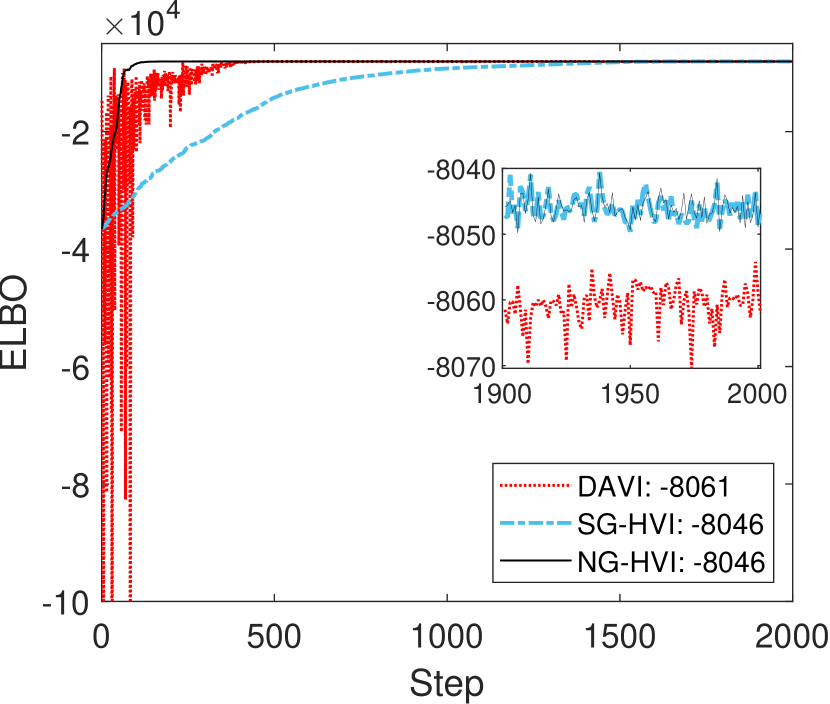
(a) Trace of ELBO against step

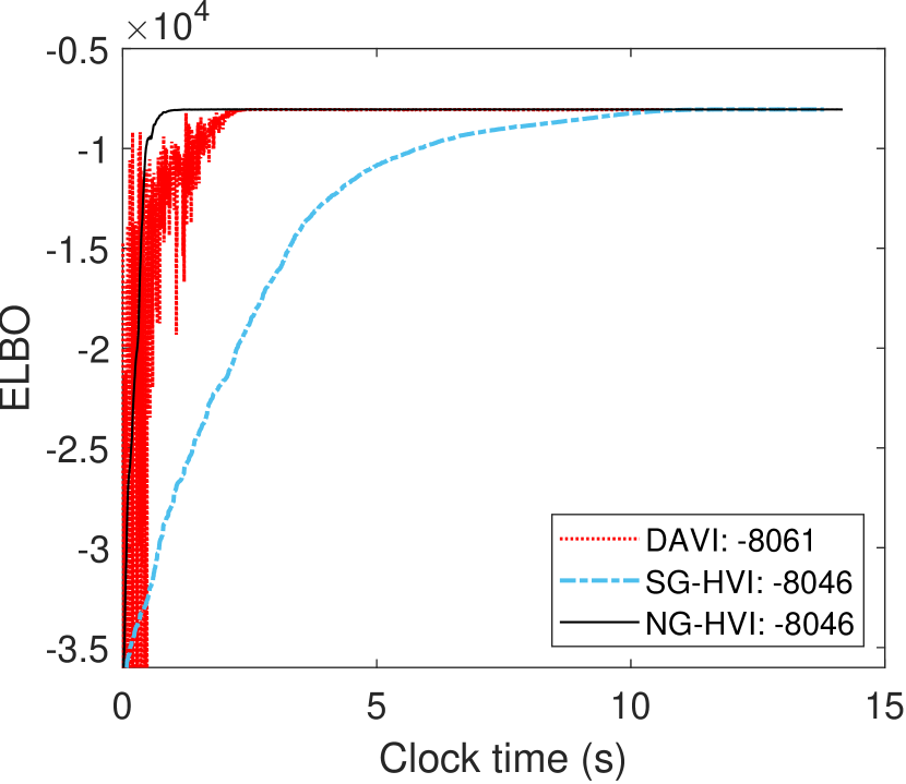
(b) Trace of ELBO against clock-time

Figure 1: Plots of the noisy ELBO function for the linear random effects regression with $\sigma^{2}_{\epsilon}=\sigma^{2}_{\alpha}=1$ and $K=1000$. Panel (a) plots against optimization step number, and panel (b) plots against wall clock time (seconds). The results for DAVI are plotted as a dotted red line, SG-HVI as a dash-dot blue line, and NG-HVI as a solid black line. The average of the noisy ELBO function values over the last 100 steps are also reported.

To compare methods we compute the noisy ELBO, which at step $t$ of the optimization is

$$\widehat{\mathcal{L}(\text{\boldmath$\lambda$}^{(t)})}=\log p(\text{\boldmath$y$}|\text{\boldmath$z$}^{(t)},\text{\boldmath$\theta$}^{(t)})+\log p(\text{\boldmath$z$}^{(t)}|\text{\boldmath$\theta$}^{(t)})+\log p(\text{\boldmath$\theta$}^{(t)})-\log q_{\lambda^{(t)}}(\text{\boldmath$\psi$}^{(t)})\,,$$ (10)

where $\text{\boldmath$\lambda$}^{(t)}$ are the variational parameters at step $t$, and $\text{\boldmath$\psi$}^{(t)}\sim q_{\lambda^{(t)}}$ is a random draw conditional on $\text{\boldmath$\lambda$}^{(t)}$. For the hybrid VI methods proposed in this paper, (10) further simplifies to $\widehat{\mathcal{L}(\text{\boldmath$\lambda$}^{(t)})}=\log p(\text{\boldmath$y$}|\text{\boldmath$z$}^{(t)},\text{\boldmath$\theta$}^{(t)})+\log p(\text{\boldmath$\theta$}^{(t)})-\log q^{0}_{\lambda^{(t)}}(\text{\boldmath$\theta$}^{(t)})$. Figure 1 plots $\widehat{\mathcal{L}(\text{\boldmath$\lambda$}^{(t)})}$ against (a) step number, and (b) clock time, for data simulated with $\sigma^{2}_{\epsilon}=\sigma^{2}_{\alpha}=1$, $K=1000$ groups and 5 data points in each group. We make four observations. First, the natural gradient methods (DAVI and NG-HVI) both converge at a much faster rate than SG-HVI. Second, NG-HVI converges faster than DAVI and to a larger value. The latter is because the VA at (1) is more accurate than that of DAVI. Third, the maximum ELBO value is the same for both SG-HVI and NG-HVI because they employ the same VA. Last, when compared to the exact posterior computed using MCMC, the variational posteriors from NG-HVI are more accurate than those from DAVI; see Part C of the Web Appendix.

Datasets were generated using different values of $K$ and ratios $\sigma^{2}_{\alpha}/\sigma^{2}_{\epsilon}$, and the accuracy of DAVI and NG-HVI measured by the average of $\widehat{\mathcal{L}(\text{\boldmath$\lambda$}^{(t)})}$ over the last 100 steps of the NGA algorithms. Table 1 reports these values for DAVI, along with the difference with NG-HVI. The latter is computed for $p\in\{0,1,2,3\}$ factors for the Gaussian factor approximation $q^{0}$ to illustrate the robustness of the hybrid VI method. The case $p=0$ corresponds to a mean field Gaussian approximation for the marginal VA in $\theta$, although we stress this is not a mean field approximation for $\psi$. NG-HVI is more accurate than DAVI, with the improvement being greatest for $K=1000$. The choice of $p$ has little impact on the NG-HVI results, with only slightly higher ELBO values for larger $p$. Further details on this example can be found in Part C of the Web Appendix.

Table 1: Improvement in ELBO of NG-HVI over DAVI for different DGP settings and number of factors $p$.

DGP Setting		$ELBO_{DAVI}$		$ELBO_{HVI}-ELBO_{DAVI}$
$K$	$\sigma^{2}_{\alpha}/\sigma^{2}_{\epsilon}$			$p=0$	$p=1$	$p=2$	$p=3$
100	$0.01$	-7327.1		6.2	7.0	7.2	7.7
	$1$	-7470.1		2.9	3.7	3.7	4.2
	$10$	-7583.8		0.7	1.2	1.9	2.1
500	$0.01$	-7234.9		8.1	8.4	9.1	8.9
	$1$	-7787.3		5.8	6.1	6.6	6.4
	$10$	-8340.4		1.9	2.4	3.4	2.9
1000	$0.01$	-7242.6		46.5	47.3	47.3	47.5
	$1$	-8061.0		14.1	14.8	14.7	14.8
	$10$	-9155.7		17.5	17.9	18.3	18.5

Note: Positive numbers in the last four columns indicate improved accuracy of NG-HVI relative to DAVI.

4 Hybrid Variational Inference for Deep Mixed Models

4.1 Deep mixed models

Bayesian neural networks are probabilistic neural networks estimated using Bayesian inference; see Jospin et al., (2022) for an introduction. Following Tran et al., (2020), we consider a Bayesian neural network with random output layer coefficients to allow for group-level heterogeneity, which these authors call a deep mixed model (DMM).

For a feed forward network with $L$ layers, the DMM we consider draws observation $i$, belonging to group $k$, from

$$y_{i} \sim {\cal D}\left(f_{L+1}\left((\text{\boldmath$\beta$}+\text{\boldmath$\alpha$}_{k})^{\top}\text{\boldmath$h$}^{(L)}_{i}\right)\right)\;\mbox{ for }i=1,\dots,n$$

$$\text{\boldmath$h$}^{(l)}_{i} = f_{l}\left(W_{l}\text{\boldmath$h$}^{(l-1)}_{i}\right)\;\mbox{ for }l=1,\ldots,L\,,$$ (11)

where $f_{l}$ is an activation function, $\text{\boldmath$h$}_{i}^{(l)}$ for $l\geq 1$ is the vector of $l^{th}$ layer values for observation $i$ with the first element a constant off-set, $\text{\boldmath$h$}^{(0)}_{i}=\text{\boldmath$x$}_{i}$ is the input vector, and $W_{l}$ is the weight matrix at layer $l$. The output value $y_{i}$ has probability distribution ${\cal D}$ with parameters that are a function of $h^{(L+1)}_{i}=f_{L+1}\left((\text{\boldmath$\beta$}+\text{\boldmath$\alpha$}_{k})^{\top}\text{\boldmath$h$}^{(L)}_{i}\right)$, where we assume a linear activation function $f_{L+1}$ in our examples. The output layer coefficients are decomposed into a fixed effect term $\beta$ and a random effects term $\text{\boldmath$\alpha$}_{k}\sim N(\bm{0},\Omega_{\alpha})$ that varies over group $k=1,\ldots,K$. The random effects allow translation of the nodes from layer $L$ into the output layer to be heterogeneous over the $K$ groups. The introduction of random coefficients into the output layer of other deep neural networks is similar.

4.2 NG-HVI for DMM

The unknowns in the DMM model at (11) include weights $\text{\boldmath$w$}=(\mbox{vec}(W_{1})^{\top},\ldots,\mbox{vec}(W_{L})^{\top})^{\top}$, fixed effects $\beta$, random effects values $\text{\boldmath$\alpha$}_{1},\ldots,\text{\boldmath$\alpha$}_{K}$, covariance matrix $\Omega_{\alpha}$ and any other parameters used to specify the distribution ${\cal D}$. Bayesian estimation involves selecting priors for all unknowns and then evaluating their joint posterior distribution. The selection of appropriate priors for weights in Bayesian neural networks is an area of current research; see Tran et al., (2022) for a discussion. Here, we adopt the simple priors $\text{\boldmath$w$}\sim N(\bm{0},\sigma_{w}^{2}I)$ and $\text{\boldmath$\beta$}\sim N(\bm{0},\sigma^{2}_{\beta}I)$ with $\sigma^{2}_{w}=\sigma^{2}_{\beta}=100$. If $\mbox{dim}(\text{\boldmath$h$}_{i}^{(l)})=m_{l}$, then following Tan, (2022) a prior $\Omega_{\alpha}^{-1}\sim\mbox{Wishart}(0.01I,\nu)$ is adopted for the precision matrix, so that the prior for $\Omega_{\alpha}$ is an inverse Wishart, with $\nu=m_{L}+1$. We stress that other priors for $\text{\boldmath$w$},\text{\boldmath$\beta$},\Omega_{\alpha}$ can also be adopted just as readily when using our black box VI method.

Because $K$ is often large in practice, computation of the posterior can be challenging. However, setting $\text{\boldmath$z$}=(\text{\boldmath$\alpha$}_{1}^{\top},\ldots,\text{\boldmath$\alpha$}_{K}^{\top})^{\top}$ and $\theta$ to a vector comprising all the other unknowns, the proposed NG-HVI method is well-suited to train such DMMs. To implement step (c) of Algorithm 1, evaluation of the gradient $\nabla_{\theta}\log g(\text{\boldmath$\theta$},\text{\boldmath$z$})$ is required. The gradient with respect to $w$ can be evaluated using back-propagation (Rumelhart et al.,, 1986). We follow Tan, (2021) and re-parameterize $\Omega_{\alpha}^{-1}=LL^{\top}$ using its Cholesky factor $L=\{l_{ij}\}$ and set $l$ to a vector of the elements $\{l_{ij};j<i\}\cup\{\log(l_{ii});i=1,\ldots,m_{L}\}$. These elements are on the real line, and both the prior for $l$ and the gradient $\nabla_{l}\log g(\text{\boldmath$\theta$},\text{\boldmath$z$})$ are available in closed form; see Appendix C. The gradients with respect to the other elements of $\theta$ depend on the choice for ${\cal D}$, but are usually available either in closed form or using numerical differentiation. Another requirement to implement the algorithm is for generation from $p(\text{\boldmath$z$}|\text{\boldmath$\theta$},\text{\boldmath$y$})$ at step (b) to be feasible, which is also contingent on choice ${\cal D}$.

The implementation of NG-HVI is outlined below for two DMMs with Gaussian and Bernoulli distributions ${\cal D}$ for the output variable. The performance of the method is assessed using data simulated from two examples, where the first DGP matches the DMM fit, while the second DGP does not match the DMM fit (so that there is model mis-specification). SG-HVI and two existing natural gradient VI methods act as benchmarks. Performance is evaluated using the posterior predictive distribution, computed as outlined in Part D of the Web Appendix.

4.3 Example 2: Gaussian DMM

We generate data from the DMM at (11) with $L=2$ hidden layers, each with 5 neurons and offset (so $m_{1}=m_{2}=6$) and the ReLU activation function. The output distribution is

$$y_{i}\sim N\left((\text{\boldmath$\beta$}+\text{\boldmath$\alpha$}_{k})^{\prime}\text{\boldmath$h$}^{(2)}_{i},\sigma^{2}_{\epsilon}\right).$$ (12)

There are $K=1000$ random effect groups, with 6 observations drawn from each to form training data, and a further 2 observations drawn from each group to form test data. The input vector $\text{\boldmath$x$}_{i}$ also consists of $m_{0}=6$ values, with unity the first element and the remaining $5$ values generated from a correlated multivariate Gaussian distribution. We fix $\sigma^{2}_{\epsilon}=20$ and $\Omega_{\alpha}$ to a $6\times 6$ diagonal matrix. Further details on this DGP are given in Part D of the Web Appendix.

This DMM is estimated using SG-HVI, NG-HVI and DAVI. All three algorithms have a marginal Gaussian VA for $\theta$, where SG-HVI and NG-HVI employ a factor covariance structure with $p=3$, while DAVI uses an unrestricted covariance. We did not study how $p$ affects the accuracy of the VA, although Ong et al., 2018a found in their examples that low values were sufficient. To implement the HVI estimators, at step (b) of Algorithm 1 the density $p(\text{\boldmath$z$}|\text{\boldmath$\theta$},\text{\boldmath$y$})=\prod_{k=1}^{K}p(\text{\boldmath$\alpha$}_{k}|\text{\boldmath$\theta$},\text{\boldmath$y$})$ is a product of Gaussians, from which it is fast and simple to draw. The prior for $\sigma^{2}_{\epsilon}$ is a standard Inverse Gamma distribution with shape and scale parameters equal to 1.01. We also implemented the natural gradient algorithm of Tran et al., (2020), labeled “NAGVAC”, using the code provided by the authors, but found that in our simulated example the algorithm with default setup did not work well, so the results are not included here.

Figure 2(a) plots the noisy ELBO (10) for DAVI and the two HVI methods. The two natural gradient methods (DAVI and NG-HVI) converge in fewer steps than the first order method SG-HVI. The NG-HVI method reaches a higher maximum ELBO value after 3000 iterations. Table 2 reports the predictive accuracy from the fitted DMMs, summarized using the $R^{2}$ coefficient for both the training and test data, and NG-HVI dominates. We also optimised the model using SG-HVI with 10000 steps, and found that by using more steps SG-HVI can achieve similar results as NG-HVI.

Table 2: Predictive Accuracy for the Gaussian DMM

	Estimation Method
	DAVI	SG-HVI	SG-HVI	NG-HVI
$R^{2}_{train}$	0.7571	0.7462	0.8025	0.8047
$R^{2}_{test}$	0.5961	0.5466	0.6388	0.6332
Total steps	3000	3000	10000	3000
Time to fit (min)	25.73	2.49	8.29	2.61

Note: Computation times are for a standard laptop.

One hundred replicate datasets were generated from the DGP, and the same three methods were used to fit these datasets, with each method optimized over 3000 steps. Figure 2(b) gives boxplots of the $R^{2}$ values for the test data predictions. We conclude that the dominance NG-HVI observed for the single dataset is a robust result.

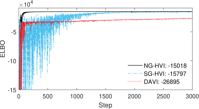
(a) Convergence of noisy ELBO.

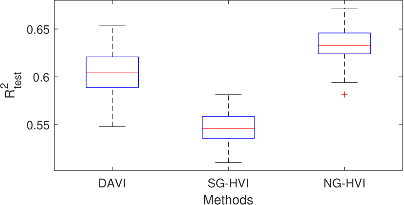
(b) Predictive Robustness

Figure 2: Simulation results from the Gaussian DMM. Panel (a) depicts convergence of the noisy ELBO against optimization step number. Panel (b) depicts boxplots of the out-of-sample predictive $R^{2}$ resulting from 100 repeated simulated datasets.

4.4 Example 3: Bernoulli DMM

In this example we compare the performance of the two HVI methods and NAGVAC. We replicate the example given in Section 6.1.4 of Tran et al., (2020), where data is generated from a Bernoulli distribution with a parameter that is a smooth nonlinear function of five covariates and a single scalar random effect; see Part D of the Web Appendix for the full specification of this DGP. The DGP deviates from the original only by the use of a logistic link function, rather than a probit link function, so as to advantage the NAGVAC estimator which employs a logistic link. There are $K=1000$ random effect groups, and from each we draw 14 observations to form training data, a further 4 observations to form test data, and an additional 4 observations as validation data to implement the NAGVAC stopping rule.

Table 3: Predictive metrics for the Bernoulli DMM

		Naive		NAGVAC		NAGVAC		SG-HVI		NG-HVI
				(stopping rule)		(no rule)
$PCE_{train}$		0.5019		0.4240		0.1238		0.1184		0.1294
$PCE_{test}$		0.6775		0.4191		0.1271		0.1355		0.1440
$F1_{train}$		0.8690		0.8959		0.9676		0.9685		0.9657
$F1_{test}$		0.8643		0.9012		0.9657		0.9620		0.9629
Time per step (secs)		–		33.59		33.59		0.48		0.50
Total steps		–		42		3000		3000		3000
Total time(min)		–		23.51		1679.45		24.23		24.88

Note: Low PCE values and high F1 values correspond to greater predictive accuracy. For the VI methods the learned Bernoulli DMMs use the variational posterior mean of the parameters. The NAGVAC method is implemented with and without the stopping rule of Tran et al., (2020). Computation times are for a standard laptop.

We use NG-HVI to learn the DMM at (11) with $L=2$ hidden layers, each with 5 neurons and an offset (so $m_{1}=m_{2}=6$), and ReLU activation functions. If $\epsilon_{i}\sim N(0,1)$, the output $y_{i}=\mathds{1}(y^{*}_{i}>0)$ is determined by the latent variable

$$y^{*}_{i}=(\text{\boldmath$\beta$}+\text{\boldmath$\alpha$}_{k})^{\prime}\text{\boldmath$h$}^{(2)}_{i}+\epsilon_{i}\,,$$

which corresponds to adopting a Bernoulli distribution for ${\cal D}$ with $f_{L+1}(x)=\Phi(x)$. Therefore, this example features model mis-specification because the DMM does not encompass the DGP.

To implement HVI, the latent variable vector is $\text{\boldmath$z$}=(\text{\boldmath$\alpha$}^{\top},\text{\boldmath$y$}^{*})$ with $\text{\boldmath$y$}^{*}=(y^{*}_{1},\ldots,y^{*}_{n})^{\top}$. At step (b) of Algorithm 1, an MCMC scheme with five sweeps is used that draws alternately from the conditional posteriors of $\alpha$ and $\text{\boldmath$y$}^{*}$, initialized at their values from the last step of the optimization. This is fast to implement, with details given in Part D of the Web Appendix. The NAGVAC algorithm is used to estimate the same DMM, but with a logistic link and $\Omega_{\alpha}$ a diagonal matrix, which matches the DGP to advantage this approach.

Comparison of the different methods is based on their predictive accuracy for both the training and test data. Table 3 reports the $F1$ score and the predictive cross entropy (PCE) defined by Tran et al., (2020), where low PCE values and high F1 values correspond to greater predictive accuracy. Results for naïve predictions using group-specific proportions are provided as a benchmark. Results are provided for NAGVAC using the stopping rule given by Tran et al., (2020), and also without the rule and 3000 optimization steps. The computational time using a standard laptop is also provided for all methods. We make three observations about the Bernoulli DMMs learned using the different methods. First, using NAGVAC with stopping rule has poor accuracy. Second, while using NAGVAC without the stopping rule improved accuracy, the computing time required is excessive. Third, both HVI methods are faster and more accurate.

Figure 3: Simulation results for the Bernoulli DMM.

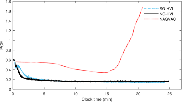
(a) Convergence of predictive cross entropy for the test data using the three methods.

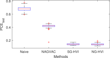
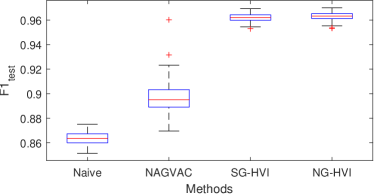
(b) Boxplots of test data posterior predictive metrics for Example 3 from 100 simulated datasets. Low PCE values and high F1 values indicate better prediction accuracy.

To further illustrate, Figure 3(b)(a) plots the PCE metric against clock time for the methods. The poor convergence of NAGVAC can be seen, as can the fast convergence of NG-HVI. To show the robustness of these results, 100 replicate datasets are generated and the methods used to learn the Bernoulli DMM for each. Figure 3(b)(b) gives boxplots of the PCE and F1 metrics for the test data. Due to the excessive computation time, only the NAGVAC results with stopping rule are given.

5 DMM for Financial Asset Pricing

There is growing interest in the use of machine learning methods for asset pricing in the financial literature (Fang and Taylor,, 2021, Feng et al.,, 2022). Compared to traditional linear models, there is evidence that neural networks can increase the predictive accuracy for asset returns (Gu et al.,, 2020), as well as there being heterogeneity across industries (Diallo et al.,, 2019, Gu et al.,, 2020).

To explore both features, we estimate Gaussian DMMs with the output layer given at (12), and either the three factors of Fama and French, (1993) (hereafter “FF3”), or the five factors of Fama and French, (2015) (hereafter “FF5”), as inputs. The three factors in FF3 are the excess market return (ERM), a firm size factor (SMB) and a value premium (HML). The five factors in FF5 extends these to include a firm profitability factor (RMW) and an firm investment strategy factor (CMA). The random effect groups are defined by the 4-digit Security Industry Code (SIC), so that the DMM captures industry variation in the factor risk premia. Two architectures are used. The first has one hidden layer of 8 neurons, and the second has 3 hidden layers of 32, 16 and 8 neurons as used by Gu et al., (2020). We do not identify an optimal architecture, and are unaware of other studies that do so for asset pricing models.

Table 4: The ten most populated 4-digit SIC groups between 2005 and 2019

SIC	Industry Description	No. of Companies
6726	Unit Investment Trusts, Face-Amount Certificate Offices,
	and Closed-End Management Investment Offices	$280$
6722	Management Investment Offices, Open-End	$116$
6798	Real Estate Investment Trusts	$100$
6020	Commercial Banks, Not Elsewhere Classified	$68$
2834	Pharmaceutical Preparations	$58$
6022	State Commercial Banks	$52$
6021	National Commercial Banks	$51$
1311	Crude Petroleum and Natural Gas	$41$
7372	Prepackaged Software	$37$
6331	Fire, Marine, and Casualty Insurance	$34$

Our output data are monthly returns between 2005 and 2019 (inclusive) for the 2583 U.S. companies in the Centre for Research in Security Prices (CRSP) database that were publicly listed during the entire period. The first 10 years are used for training, and the last 5 years for testing. The monthly factor values were obtained from the Kenneth French’s data library. In total, there are 548 industry groups, of which 260 groups feature only one company in the sample period, and 41 groups feature more than 10 companies. Table 4 summarizes the 10 most populated 4-digit SIC groups in our sample period.

Table 5: FF3 and FF5 Probabilistic Asset Pricing Models

Model Label	Model Description
Linear	Gaussian linear regression.
Random Intercept	Gaussian linear regression with random intercept.
Random Coefficients	Gaussian linear regression with random intercept and coefficients.
FNN	Deep feed forward neural network model, estimated using MATLAB “train” routine. This has a Levenberg-Marquardt training function, mean squared error performance function, and ReLU activation functions for all layers except the output layer, which uses linear activation. For probabilistic prediction the residuals are assumed independent Gaussian.
DMM	Same architecture as FNN, with random coefficients for the output layer, estimated using NG-HVI.

5.1 Predictive accuracy

Table 5 outlines five probabilistic asset pricing models. Their predictive accuracy for both the training and test data is measured using the $R^{2}$ metric for point predictions, and the log-score (LS) for probabilistic forecasts; higher values of both correspond to greater accuracy. Table 6 reports values for the five predictive models and both the FF3 and FF5 cases. Focusing on the test data results, we make four observations. First, introducing a random intercept to a linear model does not improve results, and neither does the LS improve when introducing random coefficients. Second, the FNN does not improve predictive accuracy over-and-above the traditional linear models. Third, the three hidden layer architecture dominates the shallow single layer. Last, the DMM produces a substantial improvement in predictive accuracy compared to all alternatives when using the three hidden layer architecture.

Table 6: Predictive accuracy of the five competing models.

	Fama-French 3 Factors
	$LS_{train}$	$LS_{test}$	$R^{2}_{train}$	$R^{2}_{test}$
Linear	-1.3297	-1.2502	0.1635	0.1073
Random Intercept	-1.3297	-1.2502	0.1635	0.1073
Random Coefficients	-1.3191	-1.2503	0.1953	0.1151
FNN(LM,[8])	-1.3277	-1.2589	0.1668	0.0879
DMM(NG-HVI,[8])	-1.2833	-1.2527	0.2128	0.0583
FNN(LM,[32 16 8])	-1.3319	-1.2530	0.1688	0.1011
DMM(NG-HVI,[32 16 8])	-1.2812	-1.2320	0.1934	0.1151
	Fama-French 5 Factors
	$LS_{train}$	$LS_{test}$	$R^{2}_{train}$	$R^{2}_{test}$
Linear	-1.3294	-1.2511	0.1639	0.1052
Random intercept	-1.3294	-1.2511	0.1639	0.1052
Random coefficients	-1.3178	-1.2513	0.2018	0.1051
FNN(LM,[8])	-1.3279	-1.2461	0.1665	0.1018
DMM(NG-HVI,[8])	-1.2768	-1.2477	0.2284	0.0533
FNN(LM,[32 16 8])	-1.3269	-1.2447	0.1697	0.1016
DMM(NG-HVI,[32 16 8])	-1.2871	-1.2366	0.1924	0.1118

For the FNN and DMM models two architectures are considered. The highest metric value (indicating increased accuracy) is highlighted in bold in each column.

5.2 The implied heterogeneous relationship from DMM

For the best performing DMM model, Figure 4 plots Lek profiles (Gevrey et al.,, 2003) of the FF3 factors to visualize the heterogeneous relationships for the ten most populated SIC codes given in Table 4. These depict how each factor affects expected stock returns, while the remaining factors are fixed at their values on dates that correspond to different market conditions: July 2005 (low market volatility), May 2012 (median market volatility); and October 2008 (extreme market volatility).

The profiles suggest non-linearity is not a prominent feature, but complex interactions between the factors are. There is substantial industry-based heterogeneity in the slopes. Market volatility does not seem to affect the slopes of ERM meaningfully, but does so for the other two factors. In the median market volatility case, HML has a negative slope for some industries, indicating that investors prefer high value rather than high growth stocks in these industries. Equivalent Lek profiles for the FF5 model are provided in Part E of the Web Appendix.

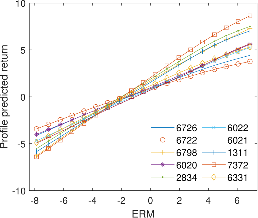
(a) ERM (low vol.)

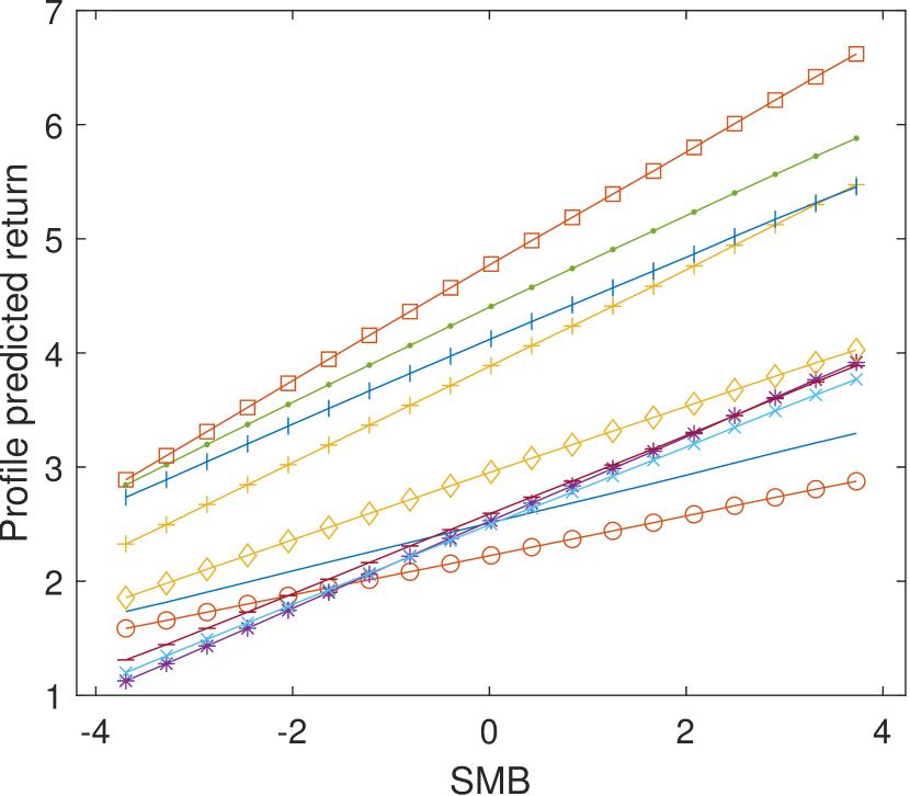
(b) SMB (low vol.)

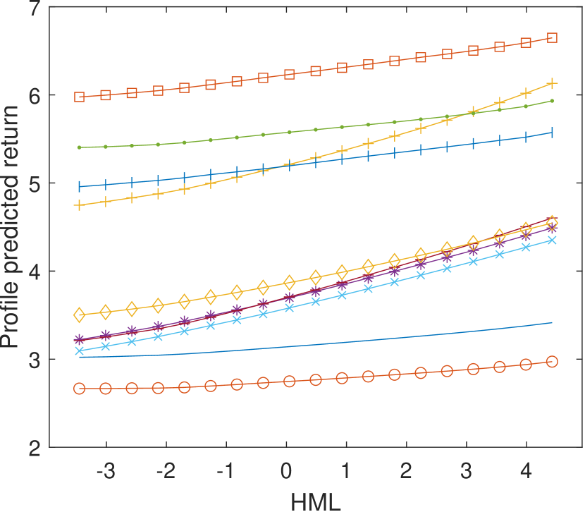
(c) HML (low vol.)

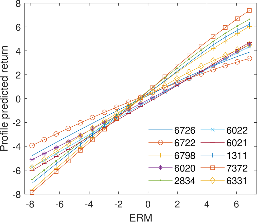
(d) ERM (median vol.)

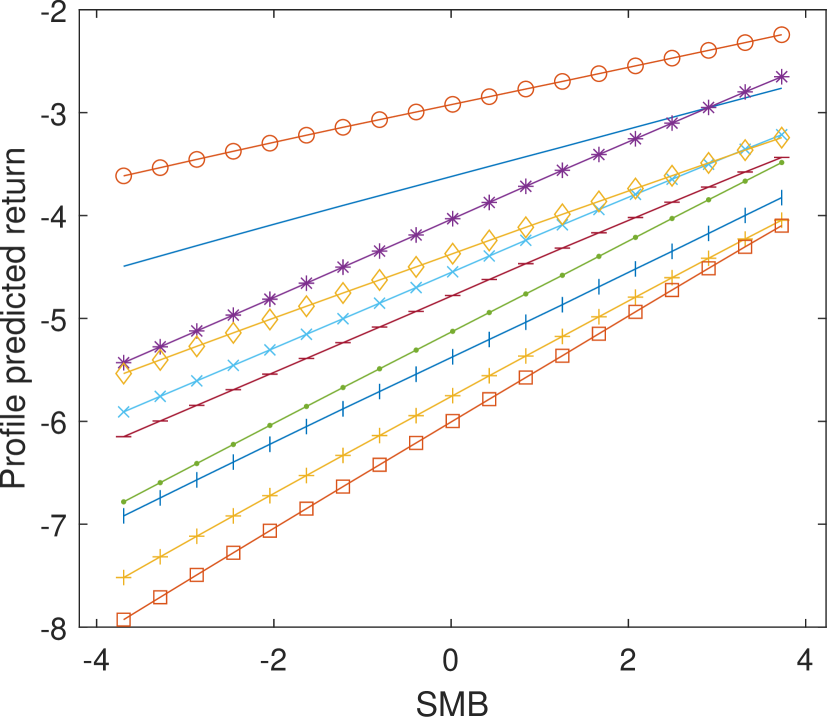
(e) SMB (median vol.)

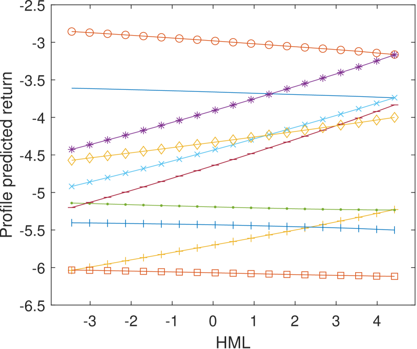
(f) HML (median vol)

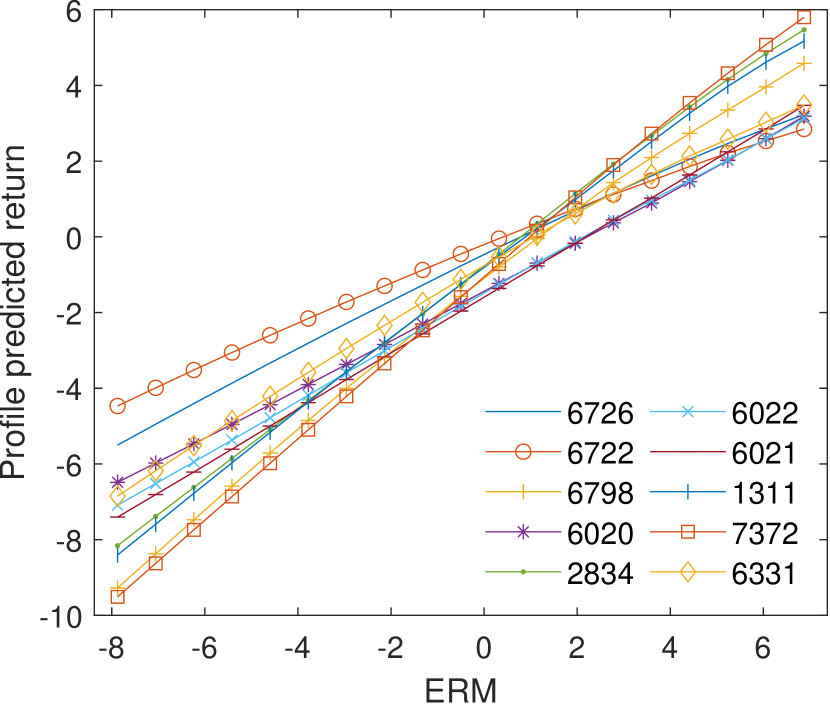
(g) ERM (extreme vol.)

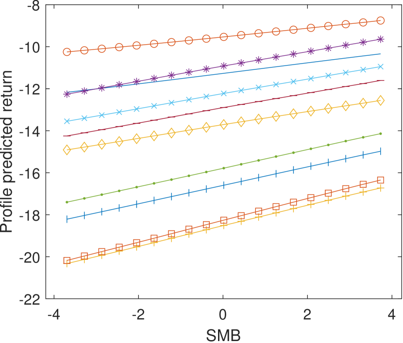
(h) SMB (extreme vol.)

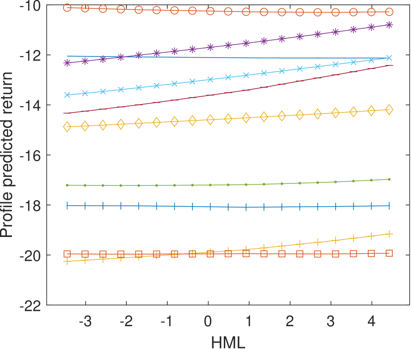
(i) HML (extreme vol.)

Figure 4: Lek profile depicting the heterogeneous responses implied by the DMM asset pricing model. The first row uses inputs on July 2005 (low market volatility month), the second row uses inputs on May 2012 (median market volatility month) and the last row inputs on October 2008 (extreme market volatility month).

6 Discussion

While natural gradient stochastic optimization methods have strong potential in variational inference, their use is limited due to the computational complexity for VAs outside the exponential family. In this paper, we propose a natural gradient method (NG-HVI) that employs the VA at (1). Doing so has three advantages which we list here. First, Theorem 1 and Corollary 1.1 show that the computational complexity of evaluating the natural gradient grows only with $\mbox{dim}(\text{\boldmath$\theta$})$, not the dimension of the target density $p(\text{\boldmath$\psi$}|\text{\boldmath$y$})$. When $\mbox{dim}(\text{\boldmath$\theta$})<<\mbox{dim}(\text{\boldmath$\psi$})$ (for example, as is the case with many latent variable models) this reduces the computational complexity of evaluating the natural gradient greatly. Second, the proposed VA may be far from Gaussian because the conditional posterior $p(\text{\boldmath$z$}|\text{\boldmath$\theta$},\text{\boldmath$y$})$ may be also. This density, nor its derivatives, are not required to implement Algorithm 1. Instead, it is only necessary to draw from this conditional posterior, which can be achieved using a wide array of existing methods. Last, that approximation at (1) is necessarily more accurate than any other VA for $\psi$ that shares the same marginal $q^{0}(\text{\boldmath$\theta$})$. In practice, the importance of this feature grows with the dimension of $z$, because the cumulative error of even well-calibrated fixed form VAs for $z$ grows as well. We demonstrate these advantages in our empirical work. The results suggest that learning the VA using SNGA proves more efficient and stable than using SGA as originally suggested by Loaiza-Maya et al., (2022). The proposed method also out-performed the two natural gradient benchmark methods for our examples. While these examples are latent variable models, NG-HVI can also be used with other stochastic models with $\psi$ partitioned in other ways, as long as generation of $z$ from its conditional posterior is viable. For example, $z$ may contain discrete-valued parameters, which is a case that is difficult to deal with using standard VI methods (Tran et al.,, 2019, Ji et al.,, 2021).

Heterogeneity is documented in many studies and using random coefficients is a popular way of capturing this (Gelman and Hill,, 2006). Thus, the DMMs proposed by Tran et al., (2020) that employ random coefficients on the output layer of a probabilistic Bayesian neural network have strong potential. However, DMMs are hard to train because the posterior is complex and the dimension of $z$ is often high. Our empirical work demonstrates that NG-HVI is an effective approach for doing so, and that it improves substantially on SG-HVI. One alternative is to use importance sampling to integrate out the random coefficients, as suggested in the original study of Tran et al., (2020). However, this is more computationally demanding than NG-HVI, and the method scales poorly with the number of output layer nodes. The potential of DMMs is demonstrated in the financial study, where the combination of a feed forward neural network and industry-based heterogeneity produces a significant increase in predictive accuracy using the Fama and French factors as inputs.

We finish by noting two directions for further work. First, while we employ the Gaussian factor covariance VA for $q^{0}$, other VAs for which fast natural gradient updates can be computed may also be used. This includes a Gaussian VA with fast Cholesky updates as suggested by Tan, (2022), the implicit copula VAs of Han et al., (2016), Smith et al., (2020), the mixture VAs of Lin et al., (2019) or the tractable fixed forms suggested by Lin et al., (2021). Second, the promising results of the financial study encourage the further exploration of the use of DMMs in asset pricing.

Appendix A Proof of Theorem 1

Observe that because $q_{\lambda}(\bm{\psi})=q^{0}_{\lambda}(\bm{\theta})p(\bm{z}|\bm{\theta},\bm{y})$, where $p(\bm{z}|\bm{\theta},\bm{y})$ is not a function of $\lambda$, then

$$F(\bm{\lambda}) =E_{q_{\lambda}}\left[\nabla_{\lambda}\log q_{\lambda}(\bm{\psi})\nabla_{\lambda}\log q_{\lambda}(\bm{\psi})^{\top}\right]$$

$$=E_{q_{\lambda}}\left[\left(\nabla_{\lambda}\log q^{0}_{\lambda}(\bm{\theta})+\nabla_{\lambda}\log p(\bm{z}|\bm{\theta},\bm{y})\right)\left(\nabla_{\lambda}\log q^{0}_{\lambda}(\bm{\theta})+\nabla_{\lambda}\log p(\bm{z}|\bm{\theta},\bm{y})\right)^{\top}\right]$$

$$=E_{q_{\lambda}}\left[\nabla_{\lambda}\log q^{0}_{\lambda}(\bm{\theta})\nabla_{\lambda}\log q^{0}_{\lambda}(\bm{\theta})^{\top}\right]$$

$$=E_{q_{\lambda}^{0}}\left[E_{p(\bm{z}|\bm{\theta},\bm{y})}\left[\nabla_{\lambda}\log q^{0}_{\lambda}(\bm{\theta})\nabla_{\lambda}\log q^{0}_{\lambda}(\bm{\theta})^{\top}\right]\right]$$

$$=E_{q_{\lambda}^{0}}\left[\nabla_{\lambda}\log q^{0}_{\lambda}(\bm{\theta})\nabla_{\lambda}\log q^{0}_{\lambda}(\bm{\theta})^{\top}\right]=F^{0}(\bm{\lambda})$$

which proves the result.

Appendix B Matrix inverse

In Section 3.3, application of the Woodbury formula and standard matrix identities provides the expression

$$\widetilde{F}_{11}(\text{\boldmath$\lambda$})^{-1} = -H^{-1}+H^{-1}G(I+G^{\top}H^{-1}G)^{-1}G^{\top}H^{-1}$$

where $H=\widetilde{E}-(1+\delta)D^{-2}$, $G=D^{-2}B\widetilde{C}$, $\widetilde{E}=-D^{-2}\mbox{diag}(\sum_{i=1}^{p}\text{\boldmath$e$}_{i}\circ\text{\boldmath$b$}_{i})D^{-2}$, $E=BC$, $C=\widetilde{C}\widetilde{C}^{\top}$, and $\widetilde{C}=(I+B^{\top}D^{-2}B)^{-1}$. The vectors $\text{\boldmath$e$}_{i}$ and $\text{\boldmath$b$}_{i}$ denote the $i^{th}$ column of matrices $E$ and $B$, respectively. Because $H$ is a diagonal matrix, no $m\times m$ matrices need to be stored to compute $\widetilde{F}_{11}(\text{\boldmath$\lambda$})^{-1}\widehat{\nabla_{\mu}{\cal L}(\text{\boldmath$\lambda$})}$.

Appendix C Prior and gradient for $l$

In Section 4.2, the precision matrix $\Omega_{\alpha}^{-1}=LL^{\top}$ is re-parameterized to $\text{\boldmath$l$}=\mbox{vech}^{\star}(L)$, where the operator ‘$\mbox{vech}^{\star}$’ is the half-vectorization of the Cholesky factor $L$, but where the logarithm is taken of the diagonal elements. The Jacobian of this transformation is easy to calculate (e.g. see Theorem 4 in Deemer and Olkin, (1951)), resulting in the prior density $p(\text{\boldmath$l$})\propto p(\Omega_{\alpha}^{-1})\prod_{i=1}^{m_{L}}l_{ii}^{(m_{L}-i+2)}$, where $p(\Omega_{\alpha}^{-1})$ is the Wishart prior for the precision matrix.

The derivative $\nabla_{l}\log g(\text{\boldmath$\theta$},\text{\boldmath$z$})=\sum_{k=1}^{K}\nabla_{l}\log p(\text{\boldmath$y$}_{k},\text{\boldmath$\alpha$}_{k}|\text{\boldmath$\theta$})+\nabla_{l}\log p(\text{\boldmath$\theta$})$. Using results from Tan, (2021),

$$\nabla_{l}\log p(\text{\boldmath$y$}_{k},\text{\boldmath$\alpha$}_{k}|\text{\boldmath$\theta$}) =D^{L}\mbox{vech}(L^{-T}-\text{\boldmath$\alpha$}_{k}\text{\boldmath$\alpha$}_{k}^{\top}L)$$

$$\nabla_{l}\log p(\text{\boldmath$\theta$}) =D^{L}\mbox{vech}\left((\nu-m_{L}-1)L^{-T}-S^{-1}L\right)+\mbox{vech}(\mbox{diag}(\text{\boldmath$u$}))\,,$$

where $D^{L}$ is a diagonal matrix of order $m_{L}(m_{L}+1)/2$ with diagonal given by $vech(J^{L})$, and $J^{L}$ is an $m_{L}\times m_{L}$ matrix with the same leading diagonal as $L$, but unity off-diagonal elements. The vector $u$ is of length $m_{L}$ with $ith$ element equal to $m_{L}-i+2$.

Online Appendix for “Natural Gradient Hybrid Varitaional Inference with Application to Deep Mixed Models”

This Online Appendix has five parts:

• Part A: Notational conventions and matrix differentiation rules used.

• Part B: Additional details on the efficient evaluation of the natural gradient.

• Part C: Additional details and empirical results for Section 3, including an additional illustrative example of a probit model.

• Part D: Additional details for the examples in Section 4.

• Part E: Additional results for the financial example in Section 5.

Part A: Notational conventions and matrix differentiation rules used
 
We outline the notational conventions that we adopt in computing derivatives throughout the paper, which are the same as adopted in Loaiza-Maya et al., (2022). For a $d$-dimensional vector valued function $g(\bm{x})$ of an $n$-dimensional argument $\bm{x}$, $\frac{\partial g}{\partial\bm{x}}$ is the $d\times n$ matrix with element $(i,j)$ $\frac{\partial g_{i}}{\partial x_{j}}$. This means for a scalar $g(\bm{x})$, $\frac{\partial g}{\partial\bm{x}}$ is a row vector. When discussing the SGA algorithm we also sometimes write $\nabla_{x}g(\bm{x})=\frac{\partial g}{\partial\bm{x}}^{\top}$, which is a column vector. When the function $g(\bm{x})$ or the argument $\bm{x}$ are matrix valued, then $\frac{\partial g}{\partial\bm{x}}$ is taken to mean $\frac{\partial\text{vec}(g(\bm{x}))}{\partial\text{vec}(\bm{x})}$, where $\text{vec}(A)$ denotes the vectorization of a matrix $A$ obtained by stacking its columns one underneath another. If $g(x)$ and $h(x)$ are matrix valued functions, say $g(x)$ takes values which are $d\times r$ and $h(x)$ takes values which are $r\times n$, then a matrix valued product rule is

$$\frac{\partial g(x)h(x)}{\partial x} =(h(x)^{\top}\otimes I_{d})\frac{\partial g(x)}{\partial x}+(I_{n}\otimes g(x))\frac{\partial h(x)}{\partial x}$$

where $\otimes$ denotes the Kronecker product and $I_{a}$ denotes the $a\times a$ identity matrix for a positive integer $a$.

Some other useful results used repeatedly throughout the derivations below are

$$\text{vec}(ABC)=(C^{\top}\otimes A)\text{vec}(B),$$

for conformable matrices $A$, $B$ and $C$ the derivative

$$\frac{\partial A^{-1}}{\partial A} =-(A^{-T}\otimes A^{-1}).$$

We also write $K_{m,n}$ for the commutation matrix (see, for example, Magnus and Neudecker, 1999).

Last, for scalar function $g(x)$ of scalar-valued argument $x$, we sometimes write $g^{\prime}(x)=\frac{d}{dx}g(x)$ and $g^{\prime\prime}(x)=\frac{d^{2}}{dx^{2}}g(x)$ for the first and second derivatives with respect to $x$ whenever it appears clearer to do so.

Part B: Additional details on the efficient evaluation of the damped natural gradient
 

Here we provide further details on the efficient evaluation of the damped natural gradient

$$\widetilde{\nabla}_{\lambda}\mathcal{L}(\bm{\lambda})\equiv\widetilde{F}^{0}(\bm{\lambda})^{-1}\widehat{\nabla_{\lambda}\mathcal{L}(\bm{\lambda})}\,,$$

for the VA at (1) with the Gaussian VA with factor covariance matrix for $q^{0}_{\lambda}$ given in Section 3.4.

First, restating the closed form expressions given in Ong et al., 2018a for the re-parameterization gradient at (7) gives

$$\nabla_{\mu}{\cal L}(\text{\boldmath$\lambda$}) = E_{f_{\varepsilon}}\left[\nabla_{\theta}\log g(\text{\boldmath$\theta$},\text{\boldmath$z$})+(BB^{\top}+D^{2})^{-1}(B\text{\boldmath$\varepsilon$}_{1}^{0}+\text{\boldmath$d$}\circ\text{\boldmath$\varepsilon$}_{2}^{0})\right]$$

$$\nabla_{\rm{vech}(B)}{\cal L}(\text{\boldmath$\lambda$}) = E_{f_{\varepsilon}}\left[\nabla_{\theta}\log g(\text{\boldmath$\theta$},\text{\boldmath$z$})(\text{\boldmath$\varepsilon$}_{1}^{0})^{\top}+(BB^{\top}+D^{2})^{-1}(B\text{\boldmath$\varepsilon$}_{1}^{0}+\text{\boldmath$d$}\circ\text{\boldmath$\varepsilon$}_{2}^{0})(\text{\boldmath$\varepsilon$}_{1}^{0})^{\top}\right]$$

$$\nabla_{d}{\cal L}(\text{\boldmath$\lambda$}) = E_{f_{\varepsilon}}\left[\mbox{diag}\left(\nabla_{\theta}\log g(\text{\boldmath$\theta$},\text{\boldmath$z$})(\text{\boldmath$\varepsilon$}_{2}^{0})^{\top}+(BB^{\top}+D^{2})^{-1}(B\text{\boldmath$\varepsilon$}_{1}^{0}+\text{\boldmath$d$}\circ\text{\boldmath$\varepsilon$}_{2}^{0})(\text{\boldmath$\varepsilon$}_{2}^{0})^{\top}\right)\right]\,,$$

where ${\rm diag}(A)$ is the vector of diagonal elements of the square matrix $A$. The expectations are evaluated at a single draw from the density

$$\text{\boldmath$\varepsilon$}=\left((\text{\boldmath$\varepsilon$}^{0}_{1})^{\top},(\text{\boldmath$\varepsilon$}^{0}_{2})^{\top},\text{\boldmath$z$}^{\top}\right)^{\top}\sim f_{\text{\boldmath$\varepsilon$}}(\text{\boldmath$\varepsilon$}^{0},\text{\boldmath$z$})=f_{\text{\boldmath$\varepsilon$}^{0}}(\text{\boldmath$\varepsilon$}^{0})p(\text{\boldmath$z$}|h(\text{\boldmath$\varepsilon$}^{0},\text{\boldmath$\lambda$}),\text{\boldmath$y$})\,,$$

with $\text{\boldmath$\varepsilon$}^{0}=((\text{\boldmath$\varepsilon$}_{1}^{0})^{\top},(\text{\boldmath$\varepsilon$}_{2}^{0})^{\top})^{\top}$, the transformation $h(\text{\boldmath$\varepsilon$}^{0},\text{\boldmath$\lambda$})=\text{\boldmath$\mu$}+B\text{\boldmath$\varepsilon$}_{1}^{0}+\text{\boldmath$d$}\circ\text{\boldmath$\varepsilon$}_{2}^{0}$ and $f_{\varepsilon_{0}}$ is the density of a $N(\bm{0},I_{m+p})$ distribution. Generating from $p(\text{\boldmath$z$}|h(\text{\boldmath$\varepsilon$}^{0},\text{\boldmath$\lambda$}),\text{\boldmath$y$})$ is undertaken either directly using a Monte Carlo method, or approximately using a few steps of an MCMC scheme initialized at the draw of $z$ obtained at the previous step of the NGA algorithm. In the computations above, the $m\times m$ matrix $(BB^{\top}+D^{2})^{-1}$ is not evaluated or stored directly, but is replaced by the Woodbury formula $(BB^{\top}+D^{2})^{-1}=D^{-2}-D^{-2}B(I+B^{\top}D^{-2}B)^{-1}B^{\top}D^{-2}$ in the equations. Multiplying through enables efficient evaluation.

Second, to evaluate the damped FIM, we first note that for the Gaussian factor covariance VA for $q^{0}_{\lambda}$, the FIM $F^{0}$ is given by the patterned matrix at (8). Ong et al., 2018b give the following closed form expressions for the block matrices:

$$F_{11}(\text{\boldmath$\lambda$}) = (BB^{\top}+D^{2})^{-1}$$

$$F_{22}(\text{\boldmath$\lambda$}) = 2(B^{\top}\Sigma^{-1}B\otimes\Sigma^{-1})$$

$$F_{33}(\text{\boldmath$\lambda$}) = 2(D\Sigma^{-1}\circ\Sigma^{-1}D)$$

$$F_{32}(\text{\boldmath$\lambda$}) = 2(B^{\top}\Sigma^{-1}D\otimes\Sigma^{-1})E_{m}^{\top}$$

where $E_{m}$ is an $m\times m^{2}$ permutation matrix such that for an $m\times m$ matrix $A$, $E_{m}\mbox{vec}(A)=\mbox{diag}(A)$.

The damped FIM is equal to (8), but with the leading diagonal blocks replaced by $\widetilde{F}_{jj}(\text{\boldmath$\lambda$})=F_{jj}(\text{\boldmath$\lambda$})+\delta\mbox{diag}\left(F_{jj}(\text{\boldmath$\lambda$})\right)$ for $j=1,2,3$. The elements $\widetilde{F}_{11}(\text{\boldmath$\lambda$})^{-1}\widehat{\nabla_{\mu}{\cal L}(\text{\boldmath$\lambda$})}$ are computed using the analytical expression for $\widetilde{F}_{11}(\text{\boldmath$\lambda$})^{-1}$ given in Appendix B of the paper. The remaining elements of the damped natural gradient are obtained by using a pre-conditioned conjugate gradient solver (such as “pcg” in MATLAB) to solve the system

$$\left[\begin{array}[]{cc}\widetilde{F}_{22}(\text{\boldmath$\lambda$})&F_{32}(\text{\boldmath$\lambda$})^{\top}\\ F_{23}(\text{\boldmath$\lambda$})&\widetilde{F}_{33}(\text{\boldmath$\lambda$})\end{array}\right]^{-1}\left(\begin{array}[]{c}\widehat{\nabla_{\rm{vech}(B)}{\cal L}(\text{\boldmath$\lambda$})}\\ \widehat{\nabla_{d}{\cal L}(\text{\boldmath$\lambda$})}\end{array}\right)\,.$$

Part C: Additional Details for the Simulation in Section 3
 
C.1: Linear random effects model
In the random effects model we set the fixed effect vector $\text{\boldmath$\beta$}=(0.8292,-1.3250,3.9909,1.6823,-1.7564,0.5580)$, and the covariate vector $\text{\boldmath$x$}_{i}$ consists of an intercept and five values generated from a correlated Gaussian. The error variance $\sigma^{2}_{\epsilon}=1$ throughout, and the random effect variance $\sigma^{2}_{\alpha}$ is varied as outlined in Section 3.

To generate the latent variables in the HVI methods, it is straightforward to show that $p(\text{\boldmath$\alpha$}|\text{\boldmath$\theta$},\text{\boldmath$y$})=\prod_{k=1}^{K}p(\alpha_{k}|\text{\boldmath$\theta$},\text{\boldmath$y$}_{k})$, where $\alpha_{k}|\text{\boldmath$\theta$},\text{\boldmath$y$}_{k}\sim N(\mu_{\alpha_{k}},\sigma^{2}_{\alpha_{k}})$ with

$$\mu_{\alpha_{k}} =\sigma^{2}_{\alpha_{k}}\frac{\text{\boldmath$\iota$}_{k}^{\top}(\text{\boldmath$y$}_{k}-X_{k}\text{\boldmath$\beta$})}{\sigma^{2}_{e}}$$

$$\sigma^{2}_{\alpha_{k}} =\left(\frac{1}{\sigma^{2}_{\alpha}}+\frac{\text{\boldmath$\iota$}_{k}^{\top}\text{\boldmath$\iota$}_{k}}{\sigma^{2}_{e}}\right)^{-1}$$

Here $X_{k}$ and $\text{\boldmath$y$}_{k}$ are the covariate matrix and response variable corresponding to group $k$, respectively. The vector $\text{\boldmath$\iota$}_{k}$ comprises unity elements and is the same length as $\text{\boldmath$y$}_{k}$.

Computation of the exact posterior using MCMC is standard, and the exact marginal posteriors are presented in Figure A1 for the case where $\sigma^{2}_{\epsilon}=\sigma^{2}_{\alpha}=1$ and $K=1000$. Variational posterior densities are also given for the NG-HVI.The variational posteriors from NG-HVI are more accurate than those from DAVI, with the latter poorly calibrating the approximations for $\sigma^{2}_{\alpha}$ and $\sigma^{2}_{\epsilon}$ and under-estimating the variance for $\beta$. In particular, the variational posterior for the intercept coefficient $\beta_{1}$ produced by DAVI in panel (a) has very small variance.

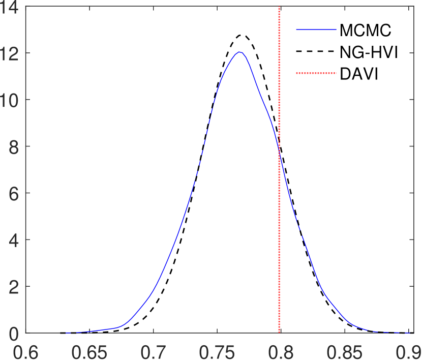
(a) posterior of $\beta_{1}$

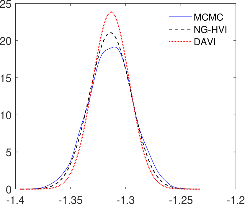
(b) posterior of $\beta_{2}$

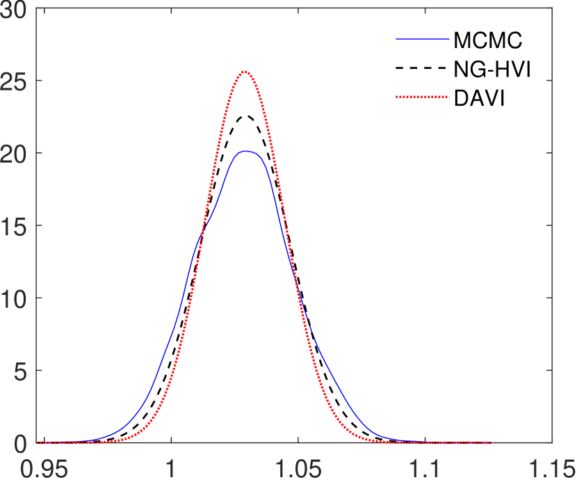
(c) posterior of $\beta_{3}$

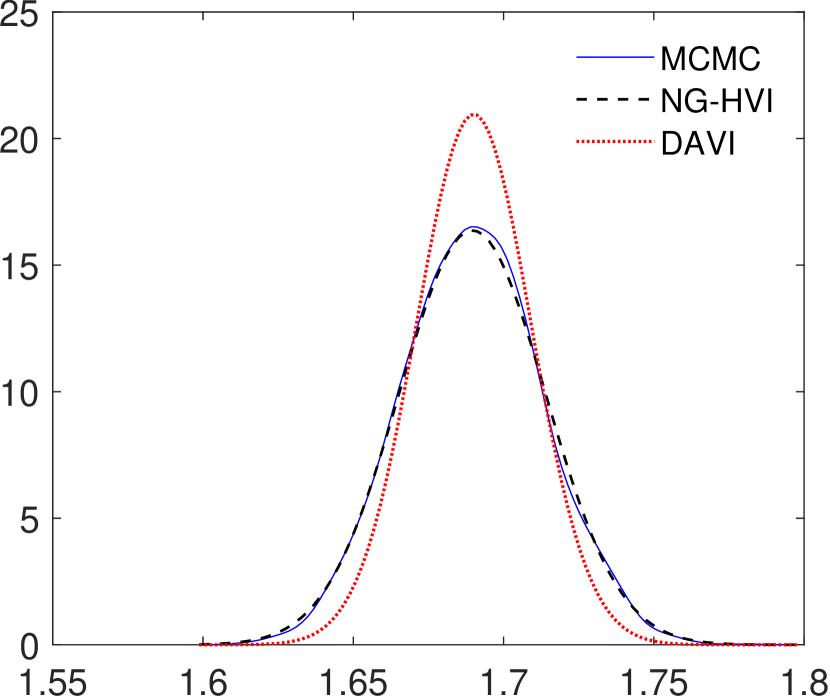
(d) posterior of $\beta_{4}$

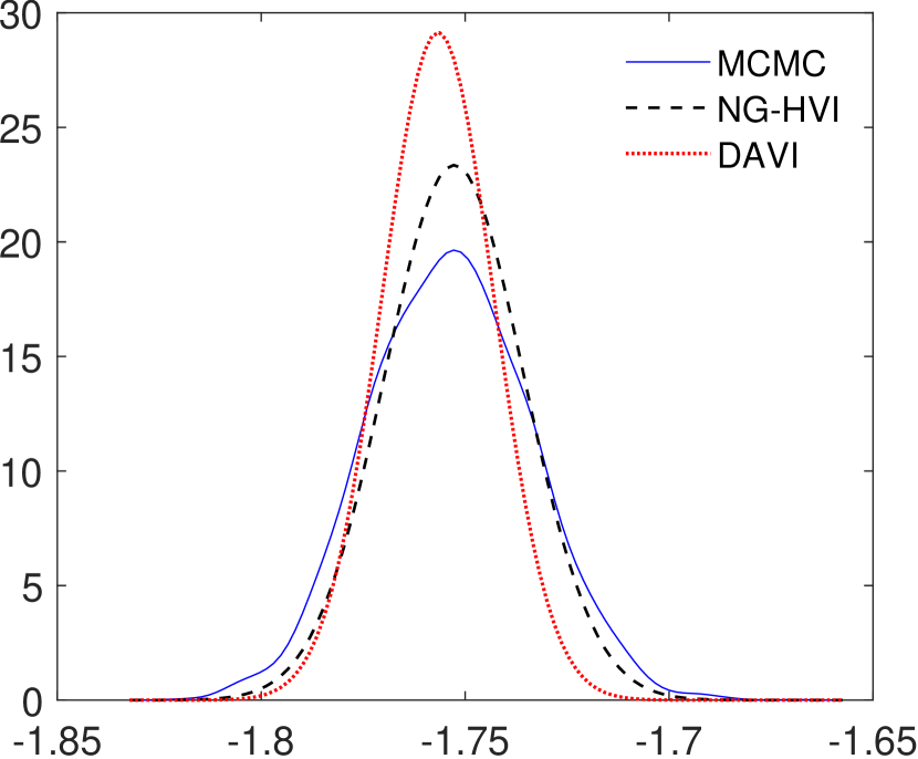
(e) posterior of $\beta_{5}$

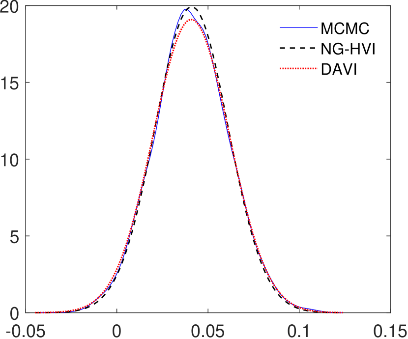
(f) posterior of $\beta_{6}$

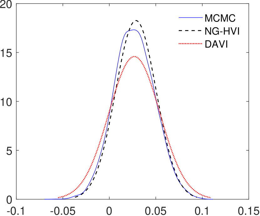
(g) Posterior density of $\log(\sigma^{2}_{\epsilon})$

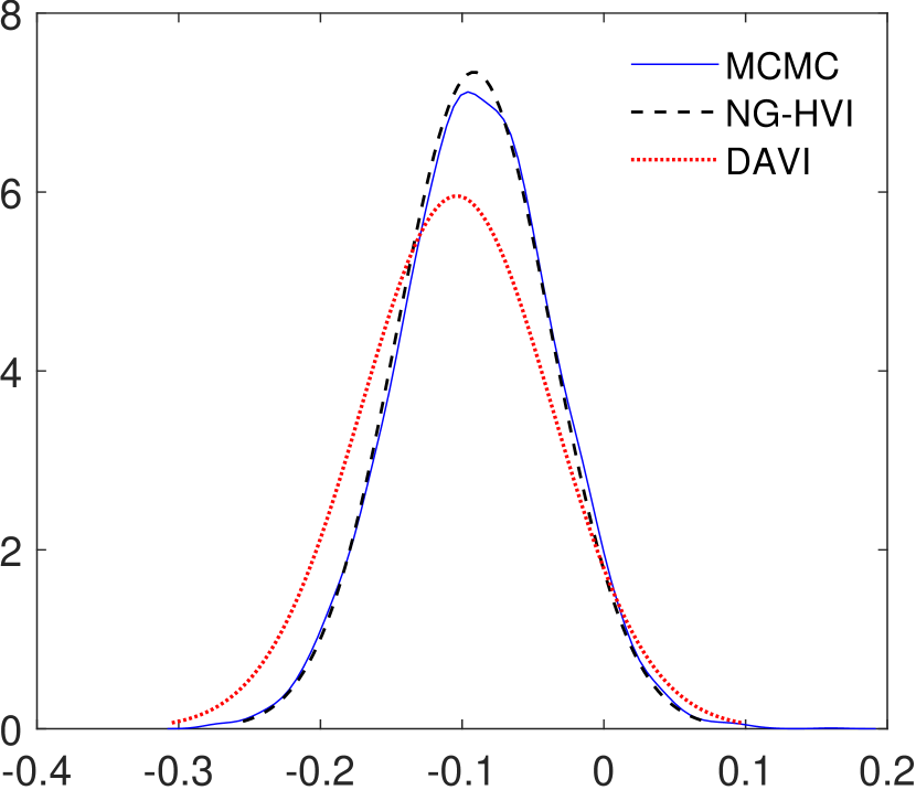
(h) Posterior density of $\log(\sigma^{2}_{\alpha})$

Figure A1: Comparison of the approximate posterior densities of the elements of $\theta$ from the VI methods and the exact posterior obtained using MCMC. These results are for the linear random effects regression when of $\sigma^{2}_{\epsilon}=\sigma^{2}_{\alpha}=1$ and $K=1000$.

C.2: Probit random effects model
We outline an additional example that extends the linear random effects model in Section 3.4 (Example 1) to a probit model with random effect. This further illustrates the increase in optimization efficiency using SNGA over SGA. Consider a probit model with a scalar random effect:

$$y_{i}^{*} =\text{\boldmath$\beta$}^{\top}\text{\boldmath$x$}_{i}+\alpha_{k}+\epsilon_{i}$$

$$y_{i} =\mathds{1}(y_{i}^{*}>0)\,,$$

where the indicator function $\mathds{1}(X)=1$ if $X$ is true, and zero otherwise, and $\epsilon_{i}\sim N(0,1)$. Following much of the random effects literature, index $k$ denotes the group membership of observation $i$.

We generate $n=2000$ observations from a DGP that has $K=100$ groups and $3$ covariates as follows:

1. Generate $\text{\boldmath$x$}^{0}_{i}\sim N_{3}(\text{\boldmath$\mu$}_{x},\Sigma_{x})$ with $\text{\boldmath$\mu$}_{x}=\mathbf{0}_{3},\Sigma_{x}=\L\L^{\prime}+diag(\text{\boldmath$d$})$, and set $\text{\boldmath$x$}_{i}=(1,\text{\boldmath$x$}^{0,\top}_{i})^{\top}$.

2. Generate $\text{\boldmath$\beta$}\sim N(\mathbf{0}_{4},10I_{4})$.

3. Generate $\alpha_{k}\sim N(0,1)$ for $k=1,\dots,100$.

4. Generate $y_{i}^{*}\sim N(\text{\boldmath$\beta$}^{\top}\text{\boldmath$x$}_{i}+\alpha_{k},1)$ and set $y_{i}=\mathds{1}(y_{i}^{*}>0)$ for $i=1,\ldots,2000$.

In this example $y_{i}^{*}$ and $\alpha_{k}$ are both latent variables, so for implementing the HVI methods we set $\text{\boldmath$z$}=(\text{\boldmath$y$}^{*\top},\text{\boldmath$\alpha$}^{\top})^{\top}$ where is $\text{\boldmath$y$}^{*}=(y_{1}^{*},y_{2}^{*},\dots,y_{n}^{*})^{\top},\text{\boldmath$\alpha$}=(\alpha_{1},\alpha_{2},\dots,\alpha_{K})^{\top}$. To generate from the distribution $\text{\boldmath$z$}|\text{\boldmath$\theta$},\text{\boldmath$y$}$ we use MCMC to generate alternately from $\text{\boldmath$\alpha$}|\text{\boldmath$y$}^{\star},\text{\boldmath$\theta$}$ and then from $\text{\boldmath$y$}^{\star}|\text{\boldmath$\alpha$},\text{\boldmath$y$}$. Generation from each is very fast because their densities are products of independent univariate Gaussian densities. We find that just five sweeps of this MCMC scheme, initialized at the values of $z$ from the last step of the stochastic optimization algorithm, provides strong results. The approach of using MCMC within SGA was explored by Loaiza-Maya et al., (2022) for more complex models and found to work well.

In this simulation, the values $\text{\boldmath$y$}^{*}$ are known. Therefore, to monitor convergence, the root mean squared error

$$RMSE=\sqrt{\frac{\sum_{i=1}^{2000}(\hat{y}_{i}^{*}-y_{i}^{*})^{2}}{2000}}$$

is computed, where $\hat{y}_{i}^{*}$ is the variational mean of the latent variable $y_{i}^{*}$. Figure A2 plots this against (a) step number of the HVI algorithm, and (b) wall clock time. By this measure, NG-HVI convergences in less than half the time required by SG-HVI.

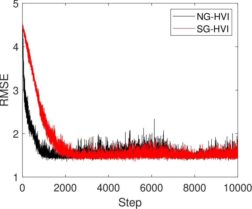
(a) Convergence of RMSE against steps

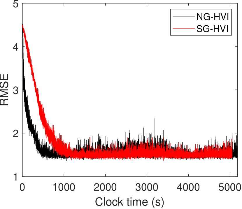
(b) Convergence of RMSE against wall clock

Figure A2: Convergence of RMSE.

Part D: Additional Details for the Examples in Section 4
 
D.1: Parameterization, priors and gradients
This section provides further details on the parameterization and choice of priors, then provides the required gradients and derivatives to implement the HVI method.

The model parameters of the Gaussian DMM in Section 4 are $\text{\boldmath$\theta$}=(\text{\boldmath$w$}^{\top},\text{\boldmath$\beta$}^{\top},\sigma^{2}_{\epsilon},\text{\boldmath$l$}^{\top})^{\top}$. For variational inference, we need to transform $\sigma^{2}_{\epsilon}$ to the real line. Thus we introduce $\theta_{\epsilon}=\log(\sigma^{2}_{\epsilon})$ and the updated model parameters are $\text{\boldmath$\theta$}=(\text{\boldmath$w$}^{\top},\text{\boldmath$\beta$}^{\top},\theta_{\epsilon},\text{\boldmath$l$}^{\top})^{\top}$. Then we have $g(\text{\boldmath$\theta$},\text{\boldmath$z$})=\prod_{k=1}^{K}\bigl{(}p(\text{\boldmath$y$}_{k}|\text{\boldmath$\alpha$}_{k},\text{\boldmath$\theta$})p(\text{\boldmath$\alpha$}_{k}|\text{\boldmath$\theta$})\bigr{)}p(\text{\boldmath$\theta$})$ with

$$p(\text{\boldmath$y$}_{k}|\text{\boldmath$\alpha$}_{k},\text{\boldmath$\theta$}) =\phi(\text{\boldmath$y$}_{k};H_{k}(\text{\boldmath$\beta$}+\text{\boldmath$\alpha$}_{k}),\sigma^{2}_{\epsilon})$$

$$P(\text{\boldmath$\alpha$}_{k}|\text{\boldmath$\theta$}) =\phi(\text{\boldmath$\alpha$}_{k};\boldmath{0},\Omega_{\alpha})$$

$$p(\text{\boldmath$w$}) =\phi(\text{\boldmath$w$};\boldmath{0},\sigma^{2}_{w}I)$$

$$p(\text{\boldmath$\beta$}) =\phi(\text{\boldmath$\beta$};\boldmath{0},\sigma^{2}_{\beta}I)$$

$$p(\theta_{\epsilon}) =\frac{b^{a}}{\Gamma(a)}\exp(\theta_{\epsilon})^{-a}\exp\bigl{(}-b\,\exp(-\theta_{\epsilon})\bigr{)}$$

$$p(\text{\boldmath$l$}) =2^{m_{L}}p(\Omega_{\alpha}^{-1})\prod_{i=1}^{m_{L}}l_{ii}^{(m_{L}-i+2)}$$

Here, $p(\theta_{\epsilon})$ was constructed by using the prior $p(\sigma^{2}_{\epsilon})=p_{IG}(\sigma^{2}_{\epsilon};a,b)$ and deriving the corresponding prior on $\theta_{\epsilon}$. The density of a $N(\text{\boldmath$\mu$},\Sigma)$ distribution is denoted as $\phi(\text{\boldmath$x$};\text{\boldmath$\mu$},\Sigma)$, and $p(\Omega_{\alpha}^{-1})$ has is the density of a Wishart distribution with degrees of freedom $\nu$ and scale matrix $0.01I$. For this example we set $\sigma^{2}_{w}=100$ and $\sigma^{2}_{\beta}=100$. $H_{k}$ is the $n_{k}\times(m_{L}+1)$ matrix with each row containing $\text{\boldmath$h$}^{(L)}_{i}$ for $i\in k$.

Given above definitions, the function $\log g(\text{\boldmath$\theta$},\text{\boldmath$z$})$ with $\text{\boldmath$z$}=(\text{\boldmath$\alpha$}_{1}^{\top},\dots,\text{\boldmath$\alpha$}_{K}^{\top})^{\top}$ can be written as:

$$\log g(\text{\boldmath$\theta$},\text{\boldmath$z$})=\sum_{k=1}^{K}\bigl{(}\log p(\text{\boldmath$y$}_{k}|\text{\boldmath$\alpha$}_{k},\text{\boldmath$\theta$})+\log p(\text{\boldmath$\alpha$}_{k}|\text{\boldmath$\theta$})\bigr{)}+\log p(\text{\boldmath$w$})+\log p(\text{\boldmath$\beta$})+\log p(\theta_{\epsilon})+\log p(\text{\boldmath$l$})$$

The gradient of $\log p(\text{\boldmath$y$}_{k}|\text{\boldmath$\alpha$}_{k},\text{\boldmath$\theta$})$ with respect to $w$ and $\beta$ can be evaluated jointly. Denote $\text{\boldmath$c$}=(\text{\boldmath$w$}^{\top},\text{\boldmath$\beta$}^{\top})$, then

$$\nabla_{c}\log p(\text{\boldmath$y$}_{k}|\text{\boldmath$\alpha$}_{k},\text{\boldmath$\theta$}) =\sigma^{-2}_{\epsilon}\nabla_{c}\text{\boldmath$\eta$}_{k}$$

$$\text{\boldmath$\eta$}_{k} =H_{k}(\text{\boldmath$\beta$}+\text{\boldmath$\alpha$}_{k})$$

$\nabla_{c}\text{\boldmath$\eta$}_{k}$ can be evaluated using standard back-propagation algorithm. The gradient of $\log p(\text{\boldmath$y$}_{k}|\text{\boldmath$\alpha$}_{k},\text{\boldmath$\theta$})$ with respect to $\theta_{\epsilon}$ can be computed as:

$$\nabla_{\theta_{\epsilon}}\log p(\text{\boldmath$y$}_{k}|\text{\boldmath$\alpha$}_{k},\text{\boldmath$\theta$}) =-\frac{1}{2}n_{k}+\frac{1}{2}\exp(-\theta_{\epsilon})(\text{\boldmath$y$}_{k}-\text{\boldmath$\eta$}_{k})^{\top}(\text{\boldmath$y$}_{k}-\text{\boldmath$\eta$}_{k})$$

See Appendix C in the manuscript for the gradient of $\log g(\text{\boldmath$\theta$},\text{\boldmath$z$})$ with respect to $l$. It is straight forward to show the following:

$$\nabla_{\text{\boldmath$w$}}\log p(\text{\boldmath$w$}) =-1/\sigma^{2}_{w}\text{\boldmath$w$}$$

$$\nabla_{\text{\boldmath$\beta$}}\log p(\text{\boldmath$\beta$}) =-1/\sigma^{2}_{\beta}\text{\boldmath$\beta$}$$

$$\nabla_{\theta_{\epsilon}}\log p(\theta_{\epsilon}) =-a+b\exp(-\theta_{\epsilon})$$

The model parameters of the Bernoulli DMM in Section 4 are $\text{\boldmath$\theta$}=(\text{\boldmath$w$}^{\top},\text{\boldmath$\beta$}^{\top},\text{\boldmath$\omega$}^{\top})^{\top}$, where $\omega$ is the non-zero elements of diagonal matrix $\Omega_{\alpha}$ with each element follows an $IG(0.1,0.1)$ distribution. Again, for variational inference we use log-transformation to transform $\omega$ to real line. The prior for $w$ and $\beta$ are normal distribution with mean $\mathbf{0}$ and $\sigma^{2}_{w}=50$, $\sigma^{2}_{\beta}=5$. The function $\log g(\text{\boldmath$\theta$},\text{\boldmath$z$})$ with $\text{\boldmath$z$}=(y_{1}^{*},\dots,y_{n}^{*},\text{\boldmath$\alpha$}_{1}^{\top},\dots,\text{\boldmath$\alpha$}_{K}^{\top})^{\top}$ is now:

$$g(\text{\boldmath$\theta$},\text{\boldmath$z$}) =\sum_{k=1}^{K}\sum_{j=1}^{n_{k}}\bigl{(}(\mathds{1}(y^{*}_{j}\leq 0,y_{j}=0)+\mathds{1}(y^{*}_{j}>0,y_{j}=1))\log p(y^{*}_{j}|\text{\boldmath$\alpha$}_{k},\text{\boldmath$\theta$})+\log p(\text{\boldmath$\alpha$}_{k}|\text{\boldmath$\theta$})\bigr{)}$$

$$\quad+\log p(\text{\boldmath$w$})+\log p(\text{\boldmath$\beta$})+\log p(\text{\boldmath$\omega$})$$

$$=\sum_{k=1}^{K}\sum_{j=1}^{n_{k}}\bigl{(}\log p(y^{*}_{j}|\text{\boldmath$\alpha$}_{k},\text{\boldmath$\theta$})+\log p(\text{\boldmath$\alpha$}_{k}|\text{\boldmath$\theta$})\bigr{)}+\log p(\text{\boldmath$w$})+\log p(\text{\boldmath$\beta$})+\log p(\text{\boldmath$\omega$})$$

$\mathds{1}(y^{*}_{j}\leq 0,y_{j}=0)+\mathds{1}(y^{*}_{j}>0,y_{j}=1)$ always sum to $1$ as $y_{i}^{*}$ is drawn from truncated normal using HVI methods, thus the second equation follows. The gradient of $\log p(y^{*}_{j}|\text{\boldmath$\alpha$}_{k},\text{\boldmath$\theta$})$ with respect to $w$ and $\beta$ again can be evaluate using back-propagation algorithm in a similar way as above, with $\sigma^{2}_{\epsilon}=1$.

D.2: Additional details on Example 2
In the data generating process (DGP) in Section 4.3, we simulated data from a DMM with two hidden layers, each with 5 neurons. The inputs $\text{\boldmath$x$}_{i}\sim N(\bm{0},V_{x})$ with

$$V_{x}=\begin{pmatrix}1&0&-0.5&0.2&0\\ 0&1&0&-0.5&0.2\\ -0.5&0&1&0&-0.5\\ 0.2&-0.5&0&1&0\\ 0&0.2&-0.5&0&1\end{pmatrix}\,,$$

and $\text{\boldmath$\alpha$}_{k}\sim N(0,\Omega_{\alpha})$ with $\Omega_{\alpha}^{-1}=diag(1.0443,9.0498,0.4569,0.5190,0.2857,2.7548)$. The output layer fixed effect coefficient vector $\text{\boldmath$\beta$}=(0.8292,-1.3250,3.9909,1.6823,-1.7564,0.5580)^{\top}$, where the first element is the offset. The hidden layer weights are fixed across simulations, with their values derived by fitting NAGVAC to the simulated dataset provided in Tran et al., (2020) and use the weighting matrices in the last step of this algorithm. We use $6$ observations from each group for training, $2$ observations from each group for testing, and another $2$ observations from each group for implementing the NAGVAC stopping rule.

To implement step (b) of Algorithm 1, the conditional posterior $\text{\boldmath$\alpha$}_{k}|\text{\boldmath$y$}_{k},\text{\boldmath$\theta$}\sim N(\text{\boldmath$\mu$}_{k},\Sigma_{k})$ with

$$\text{\boldmath$\mu$}_{k} =\Sigma_{k}H_{k}^{\top}(\text{\boldmath$y$}_{k}-H_{k}\text{\boldmath$\beta$})/\sigma^{2}_{\epsilon}$$

$$\Sigma_{k} =(\Omega_{\alpha}^{-1}+H_{k}^{\top}H_{k}/\sigma^{2}_{\epsilon})^{-1}$$

We also use NAGVAC to fit the data using the code provided by the authors with default values. This approach assumes diagonal $\Omega_{\alpha}$, which matches the DGP. It also employs a stopping rule based on improvements in predictive cross entropy (PCE) for validation data, for which we draw a further 2 observations per group from the DGP. However, we find that NAGVAC does not work well with the simulated data in this example in terms of predictive accuracy, producing negative $R^{2}$ for both in-sample and out-of-sample prediction. Thus we do not include the results of NAGVAC in this example.

D.3: Additional details on Example 3
The DGP in Example 3 in Section 4 generates $y_{i}\sim\mbox{Bernoulli}(p_{i})$ where

$$p_{i} =\frac{1}{1+exp(-\eta_{i})}$$

$$\eta_{i} =2+3(x_{i,1}-2x_{i,2})^{2}-5\left(\frac{x_{i,3}}{(1+x_{i,4})^{2}}\right)-5x_{i,5}+a_{k}\,.$$

Following Tran et al., (2020), the five covariates $x_{i,j},j=1,\dots,5$ are generated from uniform distributions $\mathcal{U}(-1,1)$ and $a_{k}\sim N(0,1)$. This DGP is the same as that suggested by these authors, except that we employ a logistic function for determining $p_{i}$, rather than a probit function. The reason for the difference is to advantage the NAGVAC algorithm which also uses a logistic link.

Both HVI methods employ an MCMC step within the SNGA optimization. For both HVI methods, we draw alternately from the conditional posterior of $\alpha$ and $y^{*}$. These both factorize into products over the groups and observations, respectively, with

$$\text{\boldmath$\alpha$}_{k}|\text{\boldmath$\theta$},\text{\boldmath$y$}_{k}^{*} \sim\mathcal{N}\left((\Omega_{\alpha}^{-1}+H_{k}^{\prime}H_{k})^{-1}H_{k}^{\prime}(\text{\boldmath$y$}_{k}^{*}-H_{k}^{\prime}\text{\boldmath$\beta$}),(\Omega_{\alpha}^{-1}+H_{k}^{\prime}H_{k})^{-1}\right)$$

$$y_{i}^{*}|\text{\boldmath$\alpha$}_{k},\text{\boldmath$\theta$},y_{i} \sim\begin{cases}TN_{(0,\infty)}(\text{\boldmath$h$}^{(L)\top}_{i}\text{\boldmath$\beta$}+\text{\boldmath$\alpha$}_{k},1)\quad\text{ if }y_{i}=1\\ TN_{(-\infty,0)}(\text{\boldmath$h$}^{(L)\top}_{i}\text{\boldmath$\beta$}+\text{\boldmath$\alpha$}_{k},1)\quad\text{ if }y_{i}=0\end{cases}$$

Here $H_{k}$ has the same definition as above, while $TN_{(a,b)}(\mu,\sigma^{2})$ represents truncated normal distribution with mean $\mu$, variance $\sigma^{2}$ and support $[a,b]$. We run this MCMC scheme for 5 sweeps, after initializing $\text{\boldmath$\alpha$},\text{\boldmath$y$}^{*}$ at their values from the last step of the optimization algorithm. The approach of using MCMC within SGA was explored by Loaiza-Maya et al., (2022) for more complex models and found to work well.

D.4: Algorithms for evaluating DMM predictive distributions

Denote $\text{\boldmath$\lambda$}^{*}$ to be the fitted variational parameter, and $X_{train}$, $\text{\boldmath$y$}_{train}$ and $n_{train}$ to be the design matrix, output vector and number of observations in the training data set, respectively. For the testing sample denote these quantities as $X_{test}$, $\text{\boldmath$y$}_{test}$ and $n_{train}$.

for $j=1:J$ do

     (1) Generate $\text{\boldmath$\theta$}^{j}\sim q_{\text{\boldmath$\lambda$}^{*}}(\text{\boldmath$\theta$})$.

     (2) Generate $\text{\boldmath$\alpha$}^{j}$ from conditional variational posterior $q_{\text{\boldmath$\lambda$}^{*}}(\text{\boldmath$\alpha$}|\text{\boldmath$\theta$}^{j})$.

     for $i=1:n_{test}$ do.

         (3.1) Set $\eta^{j}_{i}=f_{L+1}\big{(}(\text{\boldmath$\beta$}^{j}+\text{\boldmath$\alpha$}^{j}_{k})^{\top}\text{\boldmath$h$}^{(L)}_{i}\big{)}\circ f_{L}\left(W_{L}^{j}\text{\boldmath$h$}^{(L-1)}_{i}\right)\circ\dots\circ f_{1}\left(W^{j}_{1}\text{\boldmath$x$}_{test,i}\right)$.

         (3.2) Set $p^{j}_{i}=\phi(y_{i};\eta^{j}_{i},\sigma_{\epsilon}^{2,j})$.

     end for

end for

for $i=1:n_{test}$ do

     (4.1) $\hat{y}_{i}=\frac{1}{J}\sum_{j=1}^{J}\eta^{j}_{i}$.

     (4.2) $\hat{p}_{i}=\frac{1}{J}\sum_{j=1}^{J}p^{j}_{i}$.

end for

(5.1) $R^{2}_{test}=1-\frac{\sum_{i=1}^{n_{test}}(y_{i}-\hat{y}_{i})^{2}}{\sum_{i=1}^{n_{test}}(y_{i}-\bar{y})^{2}}$ with $\bar{y}=\frac{1}{n_{test}}\sum_{i=1}^{n_{test}}y_{i}$

(5.2) $RMSE_{test}=\sqrt{\sum_{i=1}^{n_{test}}(y_{i}-\hat{y}_{i})^{2}/n_{test}}$.

(5.3) $LS_{test}=\frac{1}{n_{test}}\sum_{i=1}^{n_{test}}\log{\hat{p}_{i}}$.

Algorithm 2 Evaluating performance of variational predictive distribution for Gaussian DMM

For HVI methods, we generate $\text{\boldmath$\alpha$}^{j}$ from its variational conditional posterior $p(\text{\boldmath$\alpha$}_{k}|\text{\boldmath$\theta$}^{j},X_{train},\text{\boldmath$y$}_{train})$. For DAVI we generate $\text{\boldmath$\alpha$}^{j}$ from calibrated variational approximation $q_{\text{\boldmath$\lambda$}^{*}}(\text{\boldmath$\alpha$}|\text{\boldmath$\theta$}^{j},X_{train},\text{\boldmath$y$}_{train})$. As NAGVAC integrate out $\alpha$, it does not calibrate a variational posterior for the random effects, thus we generate $\text{\boldmath$\alpha$}^{j}$ from calibrated normal distribution $N(\mathbf{0},\Omega_{\alpha}^{j})$.

Denote $\text{\boldmath$\lambda$}^{*}$ to be the fitted variational parameter, and $X_{train}$, $\text{\boldmath$y$}_{train}$ and $n_{train}$ to be the design matrix, output vector and number of observations in the training data set, respectively. For the testing sample denote these quantities as $X_{test}$, $\text{\boldmath$y$}_{test}$ and $n_{train}$.

for $j=1:J$ do

     (1) Generate $\text{\boldmath$\theta$}^{j}\sim q_{\text{\boldmath$\lambda$}^{*}}(\text{\boldmath$\theta$})$.

     (2) Implement the following Gibbs sampling scheme:

     for $r=1:R$ do

         (2.1) Generate ${\text{\boldmath$\alpha$}_{k}}^{j}\sim p(\text{\boldmath$\alpha$}_{k}|{\text{\boldmath$\theta$}}^{j},{\text{\boldmath$y$}^{*,j}}_{train})$ for $k=1,\dots,K$.

         (2.2) Generate $\text{\boldmath$y$}_{train,i}^{*,j}\sim p(\text{\boldmath$y$}_{train,i}^{*,j}|{\text{\boldmath$\alpha$}}^{j},{\text{\boldmath$\theta$}}^{j},\text{\boldmath$y$}_{train,i},\text{\boldmath$x$}_{train,i})$ for $i=1,\dots,n_{train}$.

     end for

     for $i=1:n_{test}$ do

         (3.1) Set $\eta^{j}_{i}=f_{L+1}\big{(}(\text{\boldmath$\beta$}^{j}+\text{\boldmath$\alpha$}^{j}_{k})^{\top}\text{\boldmath$h$}^{(L)}_{i}\big{)}\circ f_{L}\left(W_{L}^{j}\text{\boldmath$h$}^{(L-1)}_{i}\right)\circ\dots\circ f_{1}\left(W^{j}_{1}\text{\boldmath$x$}_{test,i}\right)$.

         (3.2) ${p}^{j}_{i}=\Phi(\eta^{j}_{i})$.

     end for

end for

for $i=1:n_{test}$ do

     (4.1) $\widehat{p}_{i}=\frac{1}{J}\sum_{j=1}^{J}{p}^{j}_{i}$.

     (4.2) $\widehat{y}_{i}=I(\widehat{p}_{i}>0.5)$.

end for

(5) $PCE_{test}=-\sum_{i=1}^{n_{test}}(y_{i}log(\widehat{p}_{i})+(1-y_{i})log(1-\widehat{p}_{i}))/n_{test}$.

Algorithm 3 Evaluating performance of variational predictive distribution for Bernoulli DMM

At step (2) of the above algorithm, we generate $\text{\boldmath$\alpha$}^{j}$ from calibrated normal distribution $N(\mathbf{0},\Omega_{\alpha}^{j})$ for NAGVAC, due to the same reason described above. As NAGVAC uses logit link, ${p}^{j}_{i}=1/\left(1+exp(-\eta^{j}_{i})\right)$.

E: Additional Results for Section 5.
The following figures provide Lek profiles for the FF5 model for different months that correspond to high, median and extreme volatility as measured by the VIX index.

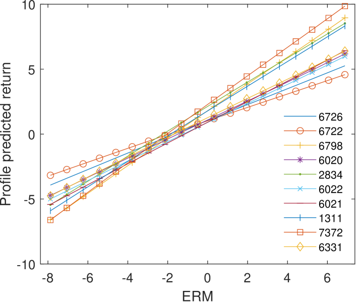
(a) ERM

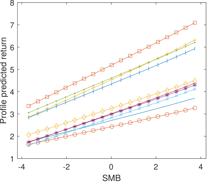
(b) SMB

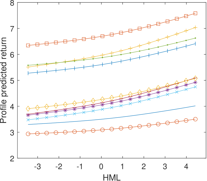
(c) HML

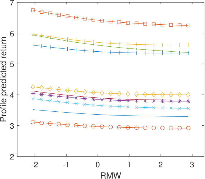
(d) RMW

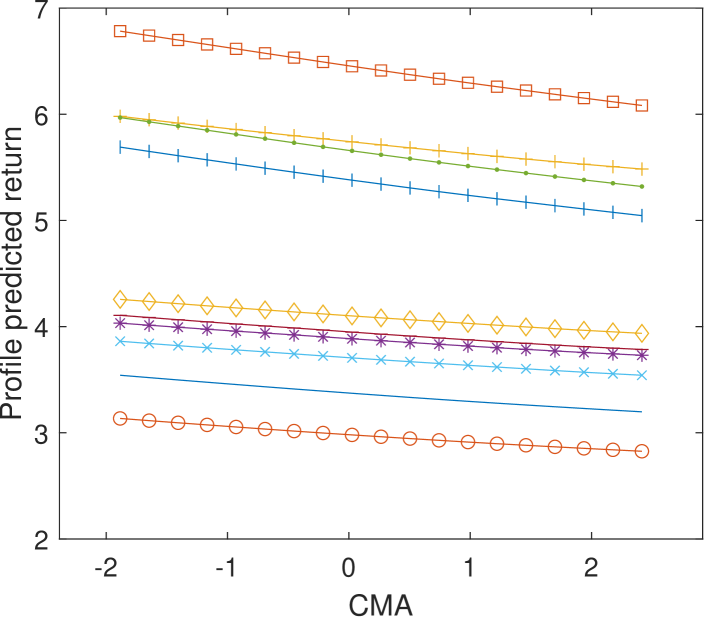
(e) CMA

Figure A3: Non-linear transformation and heterogeneity of DMM model (5FF). For July 2005 which has low level of stock market volatility (as measured by VIX index).

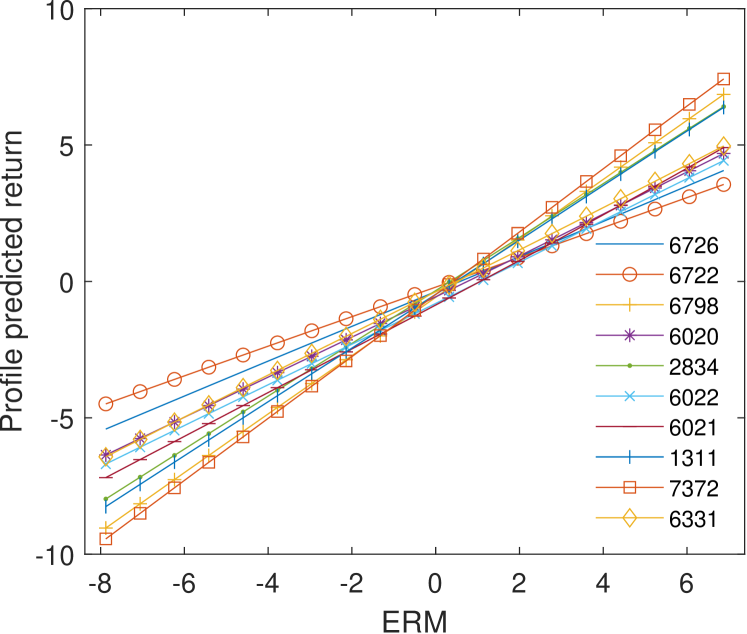
(a) ERM

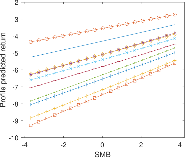
(b) SMB

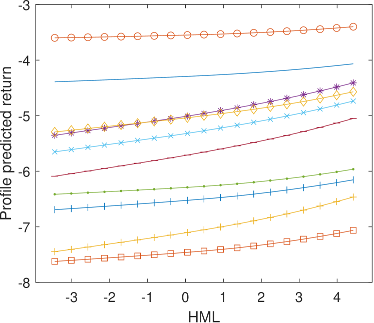
(c) HML

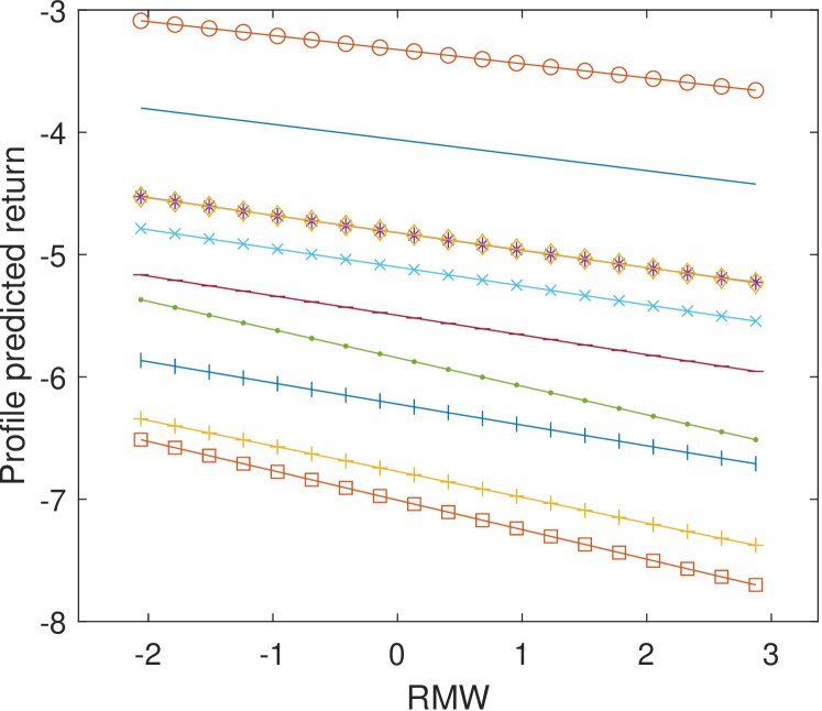
(d) RMW

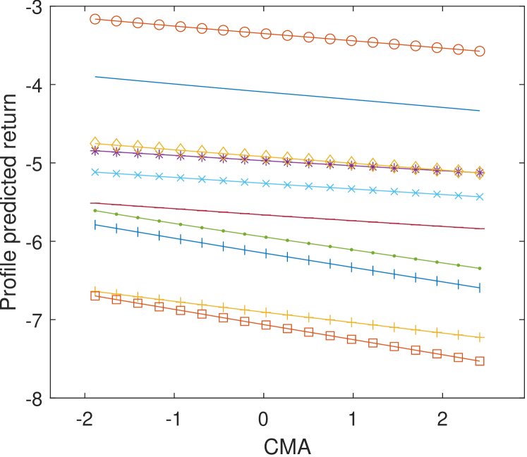
(e) CMA

Figure A4: Non-linear transformation and heterogeneity of DMM model (5FF). For May 2012 which has the median level of stock market volatility (as measured by VIX index).

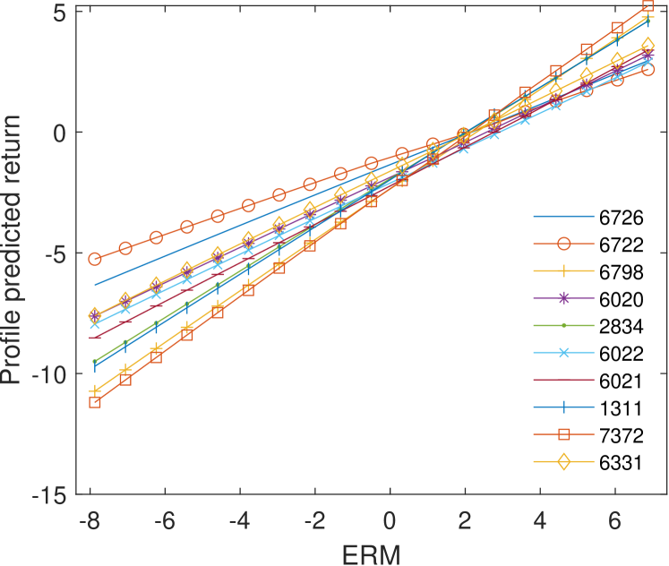
(a) ERM

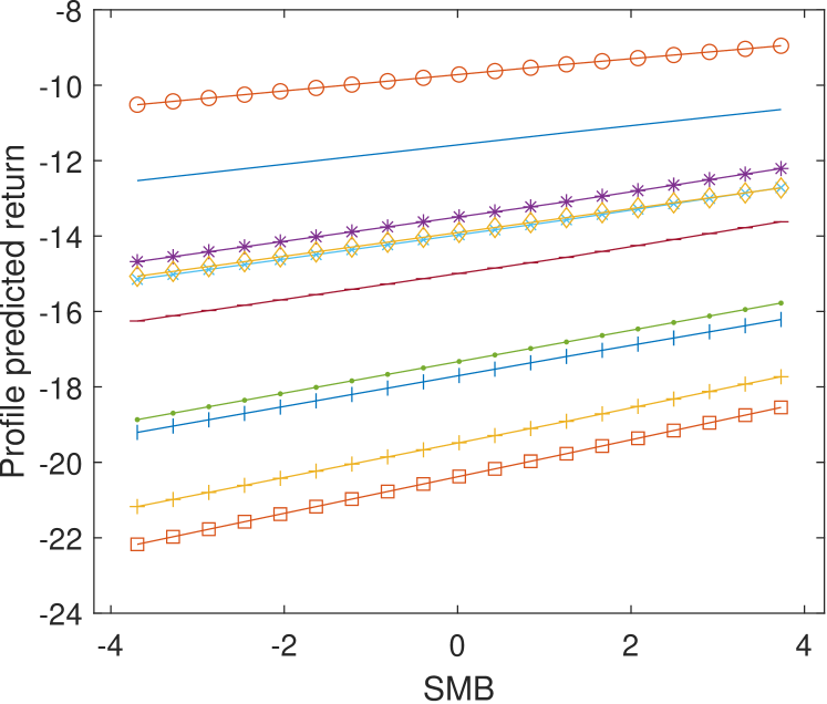
(b) SMB

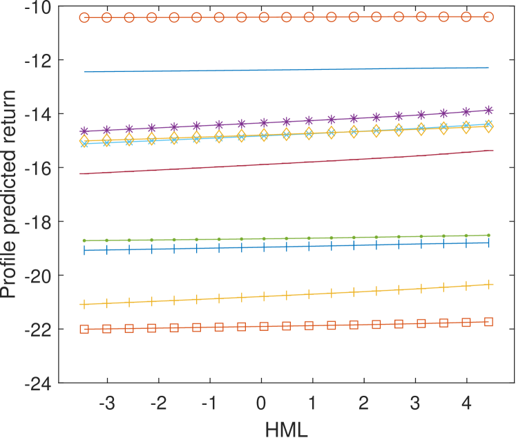
(c) HML

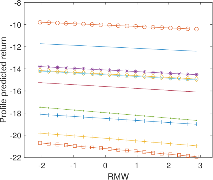
(d) RMW

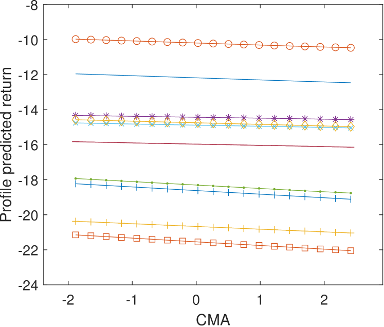
(e) CMA

Figure A5: Non-linear transformation and heterogeneity of DMM model (5FF). For October 2008 which has the highest level of stock market volatility (as measured by VIX index).

References

- Amari, (1998) Amari, S.-i. (1998). Natural Gradient Works Efficiently in Learning. Neural Computation, 10(2):251–276.
- Blei et al., (2017) Blei, D. M., Kucukelbir, A., and McAuliffe, J. D. (2017). Variational Inference: A Review for Statisticians. Journal of the American Statistical Association, 112(518):859–877.
- Blei et al., (2003) Blei, D. M., Ng, A. Y., and Jordan, M. I. (2003). Latent Dirichlet Allocation. Journal of Machine Learning Research, 3(Jan):993–1022.
- Bottou, (2010) Bottou, L. (2010). Large-scale Machine Learning with Stochastic Gradient Descent. In Lechevallier, Y. and Saporta, G., editors, Proceedings of COMPSTAT’2010, pages 177–186. Physica-Verlag HD.
- Danaher et al., (2020) Danaher, P. J., Danaher, T. S., Smith, M. S., and Loaiza-Maya, R. (2020). Advertising Effectiveness for Multiple Retailer-Brands in a Multimedia and Multichannel Environment. Journal of Marketing Research, 57(3):445–467.
- Deemer and Olkin, (1951) Deemer, W. L. and Olkin, I. (1951). The jacobians of certain matrix transformations useful in multivariate analysis: Based on lectures of PL Hsu at the University of North Carolina, 1947. Biometrika, 38(3/4):345–367.
- Diallo et al., (2019) Diallo, B., Bagudu, A., and Zhang, Q. (2019). A Machine Learning Approach to the Fama-French Three- and Five-Factor Models. Available at SSRN 3440840.
- Fama and French, (1993) Fama, E. F. and French, K. R. (1993). Common Risk Factors in the Returns on Stocks and Bonds. Journal of Financial Economics, 33(1):3–56.
- Fama and French, (2015) Fama, E. F. and French, K. R. (2015). A Five-Factor Asset Pricing Model. Journal of Financial Economics, 116(1):1–22.
- Fang and Taylor, (2021) Fang, M. and Taylor, S. (2021). A Machine Learning Based Asset Pricing Factor Model Comparison Anomaly Portfolios. Economics Letters, 204:109919.
- Feng et al., (2022) Feng, G., Polson, N. G., and Xu, J. (2022). Deep Learning in Characteristics-Sorted Factor Models. arXiv preprint arXiv:1805.01104.
- Gelman and Hill, (2006) Gelman, A. and Hill, J. (2006). Data Analysis Using Regression and Multilevel/Hierarchical Models. Analytical Methods for Social Research. Cambridge University Press.
- George et al., (2018) George, T., Laurent, C., Bouthillier, X., Ballas, N., and Vincent, P. (2018). Fast Approximate Natural Gradient Descent in a Kronecker Factored Eigenbasis. In Bengio, S., Wallach, H., Larochelle, H., Grauman, K., Cesa-Bianchi, N., and Garnett, R., editors, Advances in Neural Information Processing Systems, volume 31. Curran Associates, Inc.
- Gevrey et al., (2003) Gevrey, M., Dimopoulos, I., and Lek, S. (2003). Review and Comparison of Methods to Study the Contribution of Variables in Artificial Neural Network Models. Ecological Modelling, 160(3):249–264.
- Gu et al., (2020) Gu, S., Kelly, B., and Xiu, D. (2020). Empirical Asset Pricing via Machine Learning. The Review of Financial Studies, 33(5):2223–2273.
- Gu et al., (2021) Gu, S., Kelly, B., and Xiu, D. (2021). Autoencoder Asset Pricing Models. Journal of Econometrics, 222(1, Part B):429–450.
- Gunawan et al., (2017) Gunawan, D., Tran, M.-N., and Kohn, R. (2017). Fast Inference for Intractable Likelihood Problems using Variational Bayes. arXiv preprint arXiv:1705.06679.
- Han et al., (2016) Han, S., Liao, X., Dunson, D., and Carin, L. (2016). Variational Gaussian copula inference. In Gretton, A. and Robert, C. C., editors, Proceedings of the 19th International Conference on Artificial Intelligence and Statistics, volume 51 of Proceedings of Machine Learning Research, pages 829–838, Cadiz, Spain. PMLR.
- Hoffman and Blei, (2015) Hoffman, M. and Blei, D. (2015). Stochastic Structured Variational Inference. In Lebanon, G. and Vishwanathan, S. V. N., editors, Proceedings of the Eighteenth International Conference on Artificial Intelligence and Statistics, volume 38 of Proceedings of Machine Learning Research, pages 361–369, San Diego, California, USA. PMLR.
- Hoffman et al., (2013) Hoffman, M. D., Blei, D. M., Wang, C., and Paisley, J. (2013). Stochastic Variational Inference. The Journal of Machine Learning Research, 14(1):1303–1347.
- Honkela et al., (2010) Honkela, A., Raiko, T., Kuusela, M., Tornio, M., and Karhunen, J. (2010). Approximate Riemannian conjugate gradient learning for fixed-form variational Bayes. The Journal of Machine Learning Research, 11:3235–3268.
- Ji et al., (2021) Ji, G., Sujono, D., and Sudderth, E. B. (2021). Marginalized Stochastic Natural Gradients for Black-Box Variational Inference. In Proceedings of the 38th International Conference on Machine Learning, pages 4870–4881. PMLR. ISSN: 2640-3498.
- Jospin et al., (2022) Jospin, L. V., Laga, H., Boussaid, F., Buntine, W., and Bennamoun, M. (2022). Hands-On Bayesian Neural Networks – A Tutorial for Deep Learning Users. IEEE Computational Intelligence Magazine, 17(2):29–48. Conference Name: IEEE Computational Intelligence Magazine.
- Khan and Nielsen, (2018) Khan, M. E. and Nielsen, D. (2018). Fast yet Simple Natural-Gradient Descent for Variational Inference in Complex Models. In 2018 International Symposium on Information Theory and Its Applications (ISITA), pages 31–35, Singapore. IEEE.
- Kingma and Welling, (2014) Kingma, D. P. and Welling, M. (2014). Auto-Encoding Variational Bayes. arXiv preprint arXiv:1312.6114.
- Lin et al., (2019) Lin, W., Khan, M. E., and Schmidt, M. (2019). Fast and Simple Natural-Gradient Variational Inference with Mixture of Exponential-Family Approximations. In Chaudhuri, K. and Salakhutdinov, R., editors, Proceedings of the 36th International Conference on Machine Learning, volume 97 of Proceedings of Machine Learning Research, pages 3992–4002. PMLR.
- Lin et al., (2021) Lin, W., Nielsen, F., Emtiyaz, K. M., and Schmidt, M. (2021). Tractable structured natural-gradient descent using local parameterizations. In Proceedings of the 38th International Conference on Machine Learning, pages 6680–6691. PMLR. ISSN: 2640-3498.
- Loaiza-Maya and Smith, (2019) Loaiza-Maya, R. and Smith, M. S. (2019). Variational Bayes Estimation of Discrete-Margined Copula Models With Application to Time Series. Journal of Computational and Graphical Statistics, 28(3):523–539.
- Loaiza-Maya et al., (2022) Loaiza-Maya, R., Smith, M. S., Nott, D. J., and Danaher, P. J. (2022). Fast and Accurate Variational Inference for Models with Many Latent Variables. Journal of Econometrics, 230(2):339–362.
- Martens, (2020) Martens, J. (2020). New Insights and Perspectives on the Natural Gradient Method. Journal of Machine Learning Research, 21(146):1–76.
- Martens and Grosse, (2015) Martens, J. and Grosse, R. (2015). Optimizing Neural Networks with Kronecker-factored Approximate Curvature. In Bach, F. and Blei, D., editors, Proceedings of the 32nd International Conference on Machine Learning, volume 37 of Proceedings of Machine Learning Research, pages 2408–2417, Lille, France. PMLR.
- McCulloch and Searle, (2004) McCulloch, C. E. and Searle, S. R. (2004). Generalized, Linear, and Mixed Models. John Wiley & Sons.
- Miller et al., (2017) Miller, A. C., Foti, N. J., and Adams, R. P. (2017). Variational Boosting: Iteratively Refining Posterior Approximations. In Precup, D. and Teh, Y. W., editors, Proceedings of the 34th International Conference on Machine Learning, volume 70 of Proceedings of Machine Learning Research, pages 2420–2429. PMLR.
- Mishkin et al., (2018) Mishkin, A., Kunstner, F., Nielsen, D., Schmidt, M., and Khan, M. E. (2018). SLANG: Fast structured covariance approximations for Bayesian deep learning with natural gradient. Advances in Neural Information Processing Systems, 31.
- (35) Ong, V. M.-H., Nott, D. J., and Smith, M. S. (2018a). Gaussian Variational Approximation With a Factor Covariance Structure. Journal of Computational and Graphical Statistics, 27(3):465–478.
- (36) Ong, V. M.-H., Nott, D. J., Tran, M.-N., Sisson, S. A., and Drovandi, C. C. (2018b). Likelihood-Free Inference in High Dimensions with Synthetic Likelihood. Computational Statistics & Data Analysis, 128:271–291.
- Ormerod and Wand, (2010) Ormerod, J. T. and Wand, M. P. (2010). Explaining Variational Approximations. The American Statistician, 64(2):140–153.
- Osawa et al., (2019) Osawa, K., Tsuji, Y., Ueno, Y., Naruse, A., Yokota, R., and Matsuoka, S. (2019). Large-Scale distributed Second-Order Optimization Using Kronecker-Factored Approximate Curvature for Deep Convolutional Neural Networks. In Proceedings of the IEEE/CVF Conference on Computer Vision and Pattern Recognition, pages 12359–12367.
- Paisley et al., (2012) Paisley, J., Blei, D., and Jordan, M. (2012). Variational Bayesian inference with stochastic search. arXiv preprint arXiv:1206.6430.
- Ranganath et al., (2014) Ranganath, R., Gerrish, S., and Blei, D. (2014). Black Box Variational Inference. In Kaski, S. and Corander, J., editors, Proceedings of the Seventeenth International Conference on Artificial Intelligence and Statistics, volume 33 of Proceedings of Machine Learning Research, pages 814–822, Reykjavik, Iceland. PMLR.
- Rattray et al., (1998) Rattray, M., Saad, D., and Amari, S.-i. (1998). Natural gradient descent for on-line learning. Physical Review Letters, 81(24):5461.
- Rezende et al., (2014) Rezende, D. J., Mohamed, S., and Wierstra, D. (2014). Stochastic Backpropagation and Approximate Inference in Deep Generative Models. In Xing, E. P. and Jebara, T., editors, Proceedings of the 31st International Conference on Machine Learning, volume 32 of Proceedings of Machine Learning Research, pages 1278–1286, Bejing, China. PMLR.
- Robbins and Monro, (1951) Robbins, H. and Monro, S. (1951). A Stochastic Approximation Method. The Annals of Mathematical Statistics, 22(3):400–407.
- Rumelhart et al., (1986) Rumelhart, D. E., Hinton, G. E., and Williams, R. J. (1986). Learning Representations by Back-Propagating Errors. Nature, 323(6088):533–536.
- Simchoni and Rosset, (2021) Simchoni, G. and Rosset, S. (2021). Using random effects to account for high-cardinality categorical features and repeated measures in deep neural networks. Advances in Neural Information Processing Systems, 34:25111–25122.
- Smith et al., (2020) Smith, M. S., Loaiza-Maya, R., and Nott, D. J. (2020). High-Dimensional Copula Variational Approximation Through Transformation. Journal of Computational and Graphical Statistics, 29(4):729–743.
- Tan, (2021) Tan, L. S. L. (2021). Use of Model Reparametrization to Improve Variational Bayes. Journal of the Royal Statistical Society: Series B (Statistical Methodology), 83(1):30–57.
- Tan, (2022) Tan, L. S. L. (2022). Analytic Natural Gradient Updates for Cholesky Factor in Gaussian Variational Approximation. arXiv preprint arXiv:2109.00375.
- Tran et al., (2022) Tran, B.-H., Rossi, S., Milios, D., and Filippone, M. (2022). All you need is a good functional prior for Bayesian deep learning. Journal of Machine Learning Research, 23(74):1–56.
- Tran et al., (2019) Tran, D., Vafa, K., Agrawal, K., Dinh, L., and Poole, B. (2019). Discrete flows: Invertible generative models of discrete data. Advances in Neural Information Processing Systems, 32.
- Tran et al., (2020) Tran, M.-N., Nguyen, N., Nott, D., and Kohn, R. (2020). Bayesian Deep Net GLM and GLMM. Journal of Computational and Graphical Statistics, 29(1):97–113.
- Tran et al., (2017) Tran, M.-N., Nott, D. J., and Kohn, R. (2017). Variational Bayes with intractable likelihood. Journal of Computational and Graphical Statistics, 26(4):873–882.
- Wang et al., (2022) Wang, H., Bhattacharya, A., Pati, D., and Yang, Y. (2022). Structured Variational Inference in Bayesian State-space Models. In Camps-Valls, G., Ruiz, F. J. R., and Valera, I., editors, Proceedings of The 25th International Conference on Artificial Intelligence and Statistics, volume 151 of Proceedings of Machine Learning Research, pages 8884–8905. PMLR.
- Wikle, (2019) Wikle, C. K. (2019). Comparison of deep neural networks and deep hierarchical models for spatio-temporal data. Journal of Agricultural, Biological and Environmental Statistics, 24(2):175–203.
- Zeiler, (2012) Zeiler, M. D. (2012). ADADELTA: An Adaptive Learning Rate Method. arXiv preprint arXiv:1212.5701.
- (56) Zhang, C., Butepage, J., Kjellstrom, H., and Mandt, S. (2019a). Advances in Variational Inference. IEEE Transactions on Pattern Analysis and Machine Intelligence, 41(8):2008–2026.
- (57) Zhang, G., Martens, J., and Grosse, R. B. (2019b). Fast Convergence of Natural Gradient Descent for Over-Parameterized Neural Networks. In Advances in Neural Information Processing Systems, volume 32. Curran Associates, Inc.
- Zhang et al., (2018) Zhang, G., Sun, S., Duvenaud, D., and Grosse, R. (2018). Noisy Natural Gradient as Variational Inference. In Dy, J. and Krause, A., editors, Proceedings of the 35th International Conference on Machine Learning, volume 80 of Proceedings of Machine Learning Research, pages 5852–5861. PMLR.