Detecting Jumps on a Tree: a Hierarchical Pitman-Yor Model for Evolution of Phenotypic Distributions

Abstract

This work focuses on clustering populations with a hierarchical dependency structure that can be described by a tree. A particular example that is the focus of our work is the phylogenetic tree, with nodes often representing biological species. Clustering of the populations in this problem is equivalent to identify branches in the tree where the populations at the parent and child node have significantly different distributions. We construct a nonparametric Bayesian model based on hierarchical Pitman-Yor and Poisson processes to exploit this hierarchical structure, with a key contribution being the ability to share statistical information between subpopulations. We develop an efficient particle MCMC algorithm to address computational challenges involved with posterior inference. We illustrate the efficacy of our proposed approach on both synthetic and real-world problems.

1 Introduction

Modern datasets are characterized by rich underlying structure, resulting from the mechanistic, spatio-temporal processes that led to their generation. Trees are a widely used example, representing a hierarchical organization of observations into partially overlapping sets at multiple granularities. A classic example, and one that is the focus of this work, are phylogenetic trees used in phylogenetic comparative analyses. These show relationships between various species evolving from a common ancestor, with observations at nodes corresponding to measured phenotypes of the species. In this paper we take a broader view, and also consider evolving languages and other social norms on trees. Accounting for the underlying tree structure is important to understand relationships between and variations among the different nodes in the tree, and allows practitioners to share statistical strength between distinct but related sets of observations.

In phylogenetic comparative analyses, a number of approaches have been proposed to study the evolution of phenotypes of species whose relationship is given by a known phylogenetic tree. Many assume a single phenotype for each species, with the node values corresponding to the true means for the species. These then model the phenotypes as either evolving gradually according to some diffusion process like Brownian motion (Felsenstein, 1985; Freckleton et al., 2002; Brawand et al., 2011), or abruptly through a series of jumps, modeled by a compound Poisson process or the pure-jump part in a Levy process (Landis et al., 2012; Landis & Schraiber, 2017; Duchen et al., 2017).

In practice, the true species mean is unknown, and these approaches treat the estimated means as the true ones, known without error. This ignores within-species phenotypic variations due to measurement errors or arising from both genetic and environmental causes, leading to errors in the estimation of the model parameters (Felsenstein, 2008; Revell & Graham Reynolds, 2012). To address this issue, several authors have developed methods that take account of the intraspecific variation (Ives et al., 2007; Felsenstein, 2008; Revell & Graham Reynolds, 2012; Kostikova et al., 2016; Ansari & Didelot, 2016). These methods often allow multiple observations at each species and model them as independent and identical draws from the distribution associated with that species, with the distributions across species linked by the known phylogenetic tree. The latter linkage is achieved by allowing the phenotype distribution to evolve along the tree. Typically, the distribution at each node (i.e., species) is chosen as an element of some parametric family of probability distributions, often a Gaussian distribution for continuous phenotypes, and a categorical distribution for discrete phenotypes. The parameters of this distribution then evolve along the tree as before, again either gradually or through a jump process.

Parametric modeling approaches, while simple to work with, come with strong assumptions on the distributions of observations at each node, assumptions that are typically not satisfied in practice. A more flexible approach models these distributions with nonparametric priors that have much larger support over the space of probability distributions, and that allow modelers to approximate arbitrary multimodal distributions. An early work in this direction is that of Ansari & Didelot (2016), who considered categorical measurements, and modeled these by associating a Dirichlet distribution with each node. While the Dirichlet distribution is strictly speaking a parametric density, under mild conditions, its support includes all distributions on the associated categorical space. This opens the path to truly nonparametric priors like the Dirichlet process (Ferguson, 1973) that can approximate arbitrary probability distributions. The work of Ansari & Didelot (2016) models the evolution of the phenotype distribution with a series of Poisson distributed jumps, each jump triggering a new distribution drawn independently from a Dirichlet distribution. This assumption that the distributions before and after each jump are completely independent of each other considerably weakens the connection between species within the phylogenetic tree, and can result in less stable estimation of the model parameters at nodes with few observations. It can also make detecting small changes between distributions difficult.

In this work, we take a fully nonparametric hierarchical Bayesian approach to model evolving distributions on a phylogenetic tree. Rather than modeling the new distribution after a jump as independent of the old one, we center it at the old distribution, capturing the fact that a priori, we expect it to be similar to the old distribution. Such a hierarchical approach allows statistical sharing across nodes of the tree, so that nodes with few observations can be informed by observations across the rest of the tree, with the influence of observations waning with distance. Our work uses the Pitman-Yor process (Pitman & Yor, 1997) as its nonparametric workhorse because of a convenient marginalization property that it possesses, a property that allows us to integrate out intermediate clusters, affording computational tractability.

We organize the paper as follows. In section 2, we outlined the proposed hierarchical Pitman-Yor process (HPYP) model, and section 3 describes the novel MCMC algorithm. We apply our model to a number of synthetic and real datasets in section 4.

2 Model

We consider data consisting of collections of measurements organized along a known tree. Two specific examples are phenotypes from different species and social norms from different cultural communities. In the former, the tree represents the evolutionary history of the species under consideration, and in the latter, it might represent the historical relationship between cultures (e.g., through migration patterns). Each node in the tree, whether an internal node or a leaf, represents a population (e.g, species or community), and has associated with it a collection of zero or more observations. The branch lengths quantify the dissimilarity between parent and child populations. Denote the observed dataset as ${\mathcal{D}}=\left\{{x}_{\left(i,j\right)},~{}i=1,\dotsc,{N},~{}j=1,\dotsc,{N}_{i}\right\}$, where ${N}$ is the number of nodes and ${N}_{i}$ is the number of observations at node $i$. Often, observations are present only at the leaf nodes, corresponding for instance to measured phenotypes from present-day species, though our model allows observations at internal nodes (e.g. from measurements from fossil data).

We model the set of observations at each node as independent and identical draws from a corresponding node probability distribution, with the hierarchical dependence among these distributions determined by the tree structure. We will use ${G}_{i}$ to denote the distribution at node $i$. The distributions $G_{i}$ and $G_{j}$ at two distinct nodes $i$ and $j$ may or may not be identical. Specifically, in this work, we aim to detect significant changes in the distributions, which we represent as “jumps” distributed over the tree. Starting from the root, and moving towards the leaves, the distribution remains constant until a jump is encountered, after which a new distribution is sampled, and the process recurses. The distribution associated with any node is then the nearest distribution on the path linking it to the root.

We model the jumps as a realization of a Poisson process, so that there might be zero, one or multiple jumps on each branch of the tree. Moving down the tree from root to leaf, if there are no jumps between two nodes $i$ and $j$, then the associated distributions $G_{i}$ and $G_{j}$ are identical. It follows then that the shorter the separation between two nodes is, the more likely their associated distributions are identical. In the event of a jump, Ansari & Didelot (2016) model the new distribution $G_{new}$ as independent of the old distribution $G_{old}$; specifically, they model it as a draw from a fixed-parameter Dirichlet distribution. A more realistic assumption, and one that we make, is that the new distribution is generated from some distribution centered at the old one. This hierarchical modeling approach has two advantages. First, under the approach of Ansari & Didelot (2016), conditioned on there being at least one jump between two nodes, the distribution of the child node is independent of the actual number of jumps. By contrast, by centering the new distribution on the old one, the similarity decreases as the number of jumps increases. In particular, the new distribution continues to be centered at the old one, with variance increasing with the number of jumps. Secondly, a hierarchical modeling approach is useful in data-scarce settings, where individual nodes might have only a few observations, and it is important to pool information across multiple nodes. Under the approach of Ansari & Didelot (2016), since the new distribution is independent of the old, it can only be informed by the observations directly associated with it. This can result in a less stable estimate if only a few observations are associated with that distribution. By contrast, organizing all distributions together in a hierarchical fashion models distributions separated by fewer jumps as more similar, so that observations associated with other distributions have an influence that diminishes with separation. By shrinking the distributions towards each other, we can thus avoid overfitting, and allow better estimates.

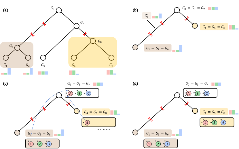
Figure 1: An example of tree node partition introduced by jumps (red crosses) and the corresponding probability distributions. (a) Color coded groups of distributions (nodes). The bar graphs show the distributions at corresponding leaf nodes. (b) The pruned tree induced by the jumps in (a), with each group represented by one node. The underlying distributions are shown by bar graphs. (c) A step in generating observations from the Chinese restaurant franchise process (see sections 2.1 and 2.2). Here, having sampled observations from the left group ${G}_{1}$ (brown) and the root group ${G}_{0}$ (white) are obtained, the first observation of the right group ${G}_{4}$ (yellow) is sampled. (d) The final clustering of all observations.

Under our modeling approach, since the distribution only changes when a jump occurs, the locations of the jumps specifies a partition of nodes, with nodes having the same distribution belonging to the same group. Consequently, tree nodes in the same group can be collapsed into a single node, with all associated observations assigned to it. We call this process pruning. Figure 1(a) clarifies these ideas through an example tree with nine nodes and their associated distributions, the root distribution ${G}_{0}$, five leaf distributions ${G}_{1},\dots,{G}_{5}$ and three internal distributions ${G}_{6}$, ${G}_{7}$ and ${G}_{8}$. It also shows the groups (color blocks) introduced by the jumps (red crosses) at two branches in the tree. Here, the distribution at root ${G}_{0}$ is the same as ${G}_{7}$ and ${G}_{3}$, so that they belong to one group. There are two jumps at the left branch of the root, but only one jump at the right branch of ${G}_{7}$, which means that the left group of populations (${G}_{1}$, ${G}_{2}$ and ${G}_{6}$) has a weaker dependence on the root distribution compared to the right group (${G}_{4}$, ${G}_{5}$ and ${G}_{8}$). Figure 1(b) demonstrates the pruned tree introduced by these jumps and the distributions associating with it, where ${G}_{1}$ represents the distribution of the left group, ${G}_{0}$ of the root, and ${G}_{4}$ represents that of the right group. Note that there is a intermediate distribution ${G}^{\prime}_{1}$ between the root and the left group ${G}_{1}$, though as we will see below, our modeling does not require us to instantiate the intermediate distributions. In this figure, like in the rest of this work, we focus on the situation where the distributions are discrete, with the bar graphs denoting discrete distributions at observed nodes, and from which observations are drawn independently.

2.1 The Hierarchical Pitman-Yor Process (HPYP) on the pruned tree

We now formalize the intuition above into a mathematical model. A key component of our model is the Pitman-Yor process (Pitman & Yor, 1997), a nonparametric prior over probability distributions. A Pitman-Yor process (PYP) is specified by a concentration parameter $\alpha$, a discount parameter ${d}\in(0,1)$ and a base probability measure ${H}$ on some space. A realization from it is a discrete probability measure ${G}$ on the same space, and can approximate arbitrary probability distributions on that space. We write this as $\left.{G}\,\middle|\,\alpha,{d},{H}\right.\sim\mathrm{Pitman\text{-}Yor}(\alpha,{d},{H}).$ The base distribution $H$ serves as the center of the prior, with $\mathbb{E}[{G}]=H$. The concentration and discount parameter satisfy $\alpha\geq-{d}$ and control the shape and spread of this prior around $H$. The Chinese restaurant process (CRP) describes the distribution of observations drawn i.i.d. from G, with G marginalized out, as follows: the first observation ${x}_{1}$ is generated directly from the base measure $H$, and conditioning on the first $j$ observations, the $(j+1)$-st observation is generated from the $K_{j}+1$-component mixture distribution

$$\left.{x}_{j+1}\,\middle|\,\{{x}_{1},\dots,{x}_{j}\},~{}\alpha,~{}{d},~{}H\right.\sim\sum_{k=1}^{K_{j}}\frac{{n}_{k}-{d}}{\alpha+j}\delta_{y_{k}}+\frac{\alpha+K_{j}\cdot{d}}{\alpha+j}H.$$ (1)

Here $K_{j}$ denotes the total number of clusters formed by the first $j$ observations, and ${n}_{k}$ and $y_{k}$ are the cluster size and the first observation of cluster $k$, respectively.

Returning to our model from the previous section, we model the root distribution $G_{0}$ as a sample from a Pitman-Yor process. Since we focus mostly on discrete spaces, we set the base distribution to the uniform distribution; on Euclidean spaces, one might set it to the Gaussian distribution. We will also use the Pitman-Yor process to model the change in distribution after each jump. Specifically, if the distribution before a jump is $G_{old}$, then the new distribution after the jump is sampled from a Pitman-Yor process whose base measure is $G_{old}$, thereby ensuring it is centered at the old distribution:

$$\left.{G}_{new}\,\middle|\,\alpha,{d},{G}_{old}\right.\sim\mathrm{Pitman\text{-}Yor}(\alpha,{d},{G}_{old}).$$

This forms a hierarchical Pitman-Yor process (HPYP) on the pruned tree.

We choose the Pitman-Yor process rather than the more well-known Dirichlet process because of a convenient marginalization property it possesses when the concentration parameter $\alpha$ is zero. This can result in significant savings when there are multiple jumps in a branch. For instance, observe the left branch in Figure 1(b), with a sequence of 3 consecutively sampled distributions $G_{0},G^{\prime}_{1}$ and $G_{1}$. With the marginalization property, $\left.{G}_{1}\,\middle|\,{G}_{0}\right.$ (with $G^{\prime}_{1}$ marginalized out) still forms a Pitman-Yor process: $\left.{G}_{1}\,\middle|\,{G}_{0}\right.\sim\mathrm{Pitman\text{-}Yor}(0,{d}^{2},{G}_{0})$. In general, on a branch with $b$ jumps, the bottom-most distribution ${G}_{child}$ is a realization of a Pitman-Yor process centered at the topmost distribution ${G}_{parent}$, with discount parameter being ${d}^{b}$:

$$\left.{G}_{child}\,\middle|\,{G}_{parent}\right.\sim\mathrm{Pitman\text{-}Yor}(0,{d}^{b},{G}_{parent}).$$ (2)

Thanks to this property, instead of having to instantiate all the intermediate measures, we can marginalize out those without any associated observations, only keeping track of the number of jumps in each branch. In Ansari & Didelot (2016), the authors do not face this issue since the new distribution is independent of the old one, so that it does not matter whether there is one or more than one jumps on a branch. We have already stated the limitations of this approach.

2.2 Chinese restaurant franchise (CRF) to generate observations

To generate observations ${\mathcal{D}}=\left\{{x}_{\left(i,j\right)},~{}i=1,\dotsc,{N},~{}j=1,\dotsc,{n}_{i}\right\}$ from HPYP, we use the Chinese restaurant franchise (CRF) (Teh et al., 2006). This is essentially a coupling of the CRPs associated with the Pitman-Yor processes on the tree nodes. Consider the node $i$ and its parent $i^{\prime}$ in the pruned tree. According to the CRP, a new sample at node $i$ either joins an existing cluster or samples a new cluster from the base measure (equation 1). Since the base measure ${G}_{i^{\prime}}$ is itself distributed as a PYP, it will have its own restaurant, with each cluster in the child nodes corresponding to a customer in this restaurant.

In general, there will be a restaurant associated with each node in the pruned tree. Following earlier notation, let ${x}_{\left(i,j\right)}$ denote the $j$-th sample at node $i$ in the CRF generative process. Denote the cluster assignment of ${x}_{\left(i,j\right)}$ by an integer $t_{\left(i,j\right)}$. We will see that generating one observation may lead, through the creation of new clusters, to latent samples being generated at ancestor nodes. To describe this, we define the cluster configuration of sample ${x}_{\left(i,j\right)}$ with a vector of varying length of the form $c_{\left(i,j\right)}=(t_{\left(i,j\right)},t_{\left(i^{\prime},j^{\prime}\right)},t_{\left(i^{\prime\prime},j^{\prime\prime}\right)},...)$, where $i^{\prime}$, $i^{\prime\prime}$, $\dots$ are the ancestor nodes of node $i$. Here, the first element, $t_{\left(i,j\right)}$, denotes the cluster joined by ${x}_{\left(i,j\right)}$ at node $i$. If $t_{\left(i,j\right)}$ represents an existing cluster, the cluster configuration $c_{\left(i,j\right)}$ will be of length 1, and there are no new clusters to be generated at the ancestor nodes. When $t_{\left(i,j\right)}$ corresponds to a new cluster, then that cluster value must be drawn from the base measure $G_{i^{\prime}}$ of node $i$. Since $G_{i^{\prime}}$ itself is PYP distributed, this cluster value corresponds to a new sample $\tilde{x}_{i^{\prime},j^{\prime}}$ from the CRP of the parent node $i^{\prime}$. Its cluster assignment $t_{\left(i^{\prime},j^{\prime}\right)}$ forms the second element of $c_{\left(i,j\right)}$. The size of $c_{\left(i,j\right)}$ continues to grow if $\tilde{x}_{i^{\prime},j^{\prime}}$ creates a new cluster leading to a new sample at its parent node. This process stops when a sample joins an existing cluster. The length of $c_{\left(i,j\right)}$ varies according to the number of new clusters generated in the process and the maximum length is the depth of node $i$.

The cluster configuration fully describes the generative process of one single observation. Applying this procedure to all observations in the pruned tree forms the full CRF process in generating the data. Since we set $\alpha=0$, the only parameter to tune in this model is the discount parameter ${d}$. Our experiment in section 4.1.1 shows that as long as it does not take values close to one, our model will perform well.

2.3 Inhomogeneous Poisson process for the jumps

As stated before, we model the jumps or changepoints as a realization of a rate-$\lambda$ Poisson process. The Poisson process can be homogeneous (with $\lambda$ a constant) or inhomogeneous, with $\lambda(p)$ varying with position $p$ on the tree. In either event, the probability of a jump in an infinitesimal interval $(p,p+\Delta p)$ on the tree is $\lambda(p)\Delta p$. A very natural approach to modeling the inhomogeneous rate involves the use of distance from the root. Here, every position $p$ on the tree has an associated time $t$, with $t$ increasing along each branch, and with the root having $t=0$. Now, the Poisson intensity is indexed by $t$, and might reflect global events that modulate the rate of jumps. Observe that for a balanced tree, the number of branches increases exponentially with $t$, and for a homogeneous Poisson process, so does the average number of jumps. Thus, a time-varying intensity function $\lambda(t)$ is also useful to control the number of jumps: by allowing it to decrease appropriately with distance from the root, one can ensure that the probability of a jump is constant over time. Since our model only cares about the number of jumps in each branch (and not their exact positions along the branch), we can also keep the jump probability constant using a homogeneous Poisson process after rescaling the branch lengths so that branches closer to the leaves are shorter. Specifically, every point on the tree is associated with a time: the distance from the root. If there are $k$ branches that share the same time tag, the jump rate at each of them needs to be scaled down by a factor of $k$ in order to have a constant jump intensity over time. Through the time-rescaling theorem, we can equivalently rescale the branch lengths, while keeping the Poisson rate constant. This is the approach we take in our experiments: it is computationally slightly simpler than simulating from an inhomogeneous Poisson process, and also allows prior distributions on the Poisson rate to be specified more easily. When learning the jump rate, we place over $\lambda$ an exponential distribution prior. The synthetic study in section 4.1.2 further investigates the performance of our model with different prior settings of the jump rate, and we find that it is generally robust to model misspecification.

Let ${\bm{b}}=({b}_{1},\dotsc,{b}_{|{\bm{b}}|})$ denote the vector of number of jumps on each branch of the tree. The full generative process for observing the data ${\mathcal{D}}=\left\{{x}_{\left(i,j\right)}\right\}$ at the nodes $i=1,\dots,{N}$ is as follows:

1. Rescale the tree branches to have a constant jump rate over time (as described above).

2. If unknown, smulate the Poisson intensity $\lambda$ from the prior. We use a weakly informative $\text{Gamma}(1,\rho)$ prior.

3. Instantiate ${\bm{b}}$ from a rate-$\lambda$ Poisson process on the rescaled tree.

4. Prune the tree according to the jumps to obtain the pruned tree, where each node represent a group of populations in the original tree with the same distribution.

5. Construct HPYP, with a PYP at each jump on the pruned tree.

6. Generate observations sequentially according to the Chinese restaurant franchise (CRF) associated with the HPYP of the pruned tree.

3 Posterior Inference

Given observations ${\mathcal{D}}=\left\{{x}_{\left(i,j\right)},~{}i=1,\dotsc,{N},~{}j=1,\dotsc,{N}_{i}\right\}$ at the nodes of the tree, we aim to recover the posterior distribution over the number and locations of jumps on the phylogenetic tree. We approximate this distribution by simulation, using a Markov chain Monte Carlo (MCMC) algorithm outlined in Algorithm 2. The state space of this algorithm are the jump configuration $\mathbf{b}$ and the jump rate $\lambda$, and the algorithm proceeds by alterately updating one given the other. In what follows, we will first give details of these update rules, before describing how the posterior samples can be used to produce point estimates of the jump locations.

1) Updating the jumps

Our MCMC algorithm begins by initializing a realization of the jumps according to the prior distribution. At each step of our sampler, we will use a Metropolis-Hastings algorithm to update the jump configuration. Specifically, given a current vector of jump counts ${\bm{b}}$ on the branches of the tree, a new proposal ${\bm{b}}^{*}$ is generated from a distribution $q\left({\bm{b}}^{*}\,\middle|\,{\bm{b}}\right)$, which is then accepted with probability $\min\{1,A({\bm{b}},{\bm{b}}^{*})\}$, where

$$A({\bm{b}},{\bm{b}}^{*}) =~{}\frac{p\left({\bm{b}}^{*}\,\middle|\,\lambda,{\mathcal{D}}\right)q\left({\bm{b}}\,\middle|\,{\bm{b}}^{*}\right)}{p\left({\bm{b}}\,\middle|\,\lambda,{\mathcal{D}}\right)q\left({\bm{b}}^{*}\,\middle|\,{\bm{b}}\right)}=~{}\frac{p\left({\mathcal{D}}\,\middle|\,{\bm{b}}^{*}\right)}{p\left({\mathcal{D}}\,\middle|\,{\bm{b}}\right)}\frac{p\left({\bm{b}}^{*}\,\middle|\,\lambda\right)q\left({\bm{b}}\,\middle|\,{\bm{b}}^{*}\right)}{p\left({\bm{b}}\,\middle|\,\lambda\right)q\left({\bm{b}}^{*}\,\middle|\,{\bm{b}}\right)}.$$ (3)

Evaluating the acceptance rate requires accessing three quantities, the proposal distribution $q\left({\bm{b}}^{*}\,\middle|\,{\bm{b}}\right)$, the prior distribution of jumps $p\left({\bm{b}}\,\middle|\,\lambda\right)$, and the data likelihood $p\left({\mathcal{D}}\,\middle|\,{\bm{b}}\right)$.

A natural choice for the proposal distribution is to first randomly select a branch and then propose the number of jumps on that branch from the prior, keeping all other elements of ${\bm{b}}$ unchanged. However, such a proposal struggles to move jumps from a branch to its parent or child. Doing so would require first introducing jumps into the parent/child node and then removing jumps from the current branch, or conversely, first removing jumps from the current branch and then introducing jumps in the parent or child branch. Both these intermediate states can have relatively low probability compared to the starting and end states, so that the MCMC algorithm can mix poorly, struggling to move between states with comparable probabilities. To address this issue, we consider an additional swap proposal, which picks two adjacent branches (a parent-child pair), and proposes exchanging the number of jumps on these, keeping the other elements of ${\bm{b}}$ unchanged. We find that randomly selecting one of these two proposal distributions each MCMC iteration dramatically improves mixing of our algorithm. For both proposal distributions, we can easily calculate $q({\bm{b}}^{*}|{\bm{b}})$ and $q({\bm{b}}|{\bm{b}}^{*})$.

The prior distribution $p\left({\bm{b}}\,\middle|\,\lambda\right)$ is simply a product of independent Poisson distributions for each branch, and is easy to evaluate. The last term $p\left({\mathcal{D}}\,\middle|\,{\bm{b}}\right)$, the probability of the data given the jumps, is however not tractable, requiring one to marginalize out all cluster configurations given the jump vector ${\bm{b}}$. We circumvent this through the pseudo-marginal approach of Andrieu et al. (2009). This recognizes that when the likelihood $p\left({\mathcal{D}}\,\middle|\,{\bm{b}}\right)$ has a positive unbiased estimator $\hat{p}\left({\mathcal{D}}\,\middle|\,{\bm{b}}\right)$, then including this in the MCMC state, and accepting a new configuration ${\bm{b}}^{*}$ with probability

$$A({\bm{b}},{\bm{b}}^{*})=\frac{\hat{p}\left({\mathcal{D}}\,\middle|\,{\bm{b}}^{*}\right)}{\hat{p}\left({\mathcal{D}}\,\middle|\,{\bm{b}}\right)}\frac{p\left({\bm{b}}^{*}\,\middle|\,\lambda\right)q\left({\bm{b}}\,\middle|\,{\bm{b}}^{*}\right)}{p\left({\bm{b}}\,\middle|\,\lambda\right)q\left({\bm{b}}^{*}\,\middle|\,{\bm{b}}\right)}$$ (4)

still yields a Metropolis-Hastings update that targets the correct distribution. To efficiently construct the unbiased estimator, we take a particle filtering approach (Andrieu et al., 2010), with each particle a realization of the latent cluster configurations $c_{(i,j)}$ of the data, and with particles updated sequentially by adding one observation at a time.

Let $S$ be the total number of particles. The particle filtering procedure starts by considering the first observation $x_{(1,1)}$, without loss of generality, we assume it belongs to node $1$. All particles are initialized as ${\mathcal{C}}^{s}_{\left(1,1\right)}=\left\{c_{\left(1,1\right)}\right\}$, $s=1,\dots,S$, with $c_{(1,1)}=(1,1,...)$. In other words, all particles assign the first observation to cluster $1$ in node $1$. As required by the CRF, this new cluster must belong to a cluster in its parent node, which forms cluster $1$ in that node, and so on, all the way up to the root node.

Now, the particles are sequentially updated, moving from observation $x_{({i},{j})}$ to incorporate the next. We use $(i,j)^{-}$ and $(i,j)^{+}$ to index observations preceding and following $(i,j)$. We denote the state of particle $s$ updated with data up until observation $(i,j)$ by $\mathcal{C}^{s}_{i,j}$, $s=1,\dots,S$. Given ${\mathcal{D}}_{\left(i,j\right)^{-}}$, observations until $(i,j)^{-}$, when the next observation $x_{\left(i,j\right)}$ is encountered, particle $s$ is expanded from the previous step by including ${c}^{s}_{\left(i,j\right)}$, a cluster configuration of ${x}_{\left(i,j\right)}$. This is sampled from the conditional distribution $p\left(c_{\left(i,j\right)}\,\middle|\,{x}_{\left(i,j\right)},{\mathcal{D}}_{\left(i,j\right)^{-}},\mathcal{C}_{\left(i,j\right)^{-}}=\mathcal{C}^{s}_{\left(i,j\right)^{-}},{\bm{b}}\right)$ This update step is a standard Gibbs update step for the CRF, described by Teh (2006) and the appendix, and is easy to implement. After all particles are updated, each will have a possibly different clustering structure for $x_{(i,j)}$ and the preceding observations. Each particle is then assigned an importance weight, with that of particle $s$ given by

$${w}^{s}_{\left(i,j\right)} =p\left({x}_{\left(i,j\right)^{+}}\,\middle|\,{\mathcal{C}}^{s}_{\left(i,j\right)},{\mathcal{D}}_{\left(i,j\right)},{\bm{b}}\right)=\sum_{c_{\left(i,j\right)^{+}}}p\left({x}_{\left(i,j\right)^{+}}\,\middle|\,c_{\left(i,j\right)^{+}},{\mathcal{C}}^{s}_{\left(i,j\right)},{\mathcal{D}}_{\left(i,j\right)}\right)p\left(c_{\left(i,j\right)^{+}}\,\middle|\,{\mathcal{C}}^{s}_{\left(i,j\right)},{\mathcal{D}}_{\left(i,j\right)}\right).$$ (5)

After computing the importance weights, particles with low weights can be eliminated by sampling the particles with replacement proportional to the importance weights. This forms the collection of particles at the end of step $\left(i,j\right)$, and the process is repeated.

Although computing the weights ${w}^{s}_{\left(i,j\right)}$ requires a full bottom to top travel of the pruned tree, this is not hard to evaluate, as $p\left({x}_{\left(i,j\right)^{+}}\,\middle|\,c_{\left(i,j\right)^{+}},\mathcal{C}_{\left(i,j\right)},{\mathcal{D}}_{\left(i,j\right)}\right)=0$ when the table configuration of the succeeding observation $c_{\left(i,j\right)^{+}}$ does not agree with its label. The weights at step $s$ also gives an unbiased estimator of the partial likelihood $p\left({x}_{\left(i,j\right)}\,\middle|\,{\mathcal{D}}_{\left(i,j\right)^{-}},{\bm{b}}\right)$,

$$\hat{p}\left({x}_{\left(i,j\right)}\,\middle|\,{\mathcal{D}}_{\left(i,j\right)^{-}},{\bm{b}}\right)=\frac{1}{S}\sum_{s=1}^{S}w^{s}_{(i,j)}.$$

and an unbiased estimator of the overall likelihood is simply the product of all the sequential estimators:

$$\hat{p}\left({\mathcal{D}}\,\middle|\,{\bm{b}}\right)=\prod_{\left(i,j\right)}\hat{p}\left({x}_{\left(i,j\right)}\,\middle|\,{\mathcal{D}}_{\left(i,j\right)^{-}},{\bm{b}}\right)$$

Algorithm 1 fully states the particle filtering algorithm, and we refer the reader to Andrieu et al. (2010) for details of the unbiasedness properties.

2) Updating the jump rate

Given the jumps ${\bm{b}}$, the conditional posterior of $\lambda$ is independent of the data, and with a Gamma$(1,\rho)$ prior, follows the Gamma distribution:

$$\left.\lambda\,\middle|\,{\bm{b}},{\mathcal{D}}\right.\sim\mathrm{Gamma}(1+\sum_{i=1}^{{|{\bm{b}}|}}{b}_{i},~{}\rho+{|{\bm{b}}|}).$$ (6)

3.1 Point estimates of the jump configuration

Our MCMC algorithm generates samples of jump configurations from the posterior distribution. We can use the MCMC samples to estimate the posterior probability that at least one jump occurs on a particular branch: this is just proportion of posterior samples whose jump configuration assigns at least one jump to that branch. While such a vector of posterior jump probabilities is a useful summary statistic, this ignores the strong correlation between jumps on different branches. For instance, a branch and its child branch might have similar posterior jump probabilities, however these might have a strong negative correlation, as any MCMC realization will have a jump on only one of the branches. In this section, we describe a novel summary statistic that accounts for such correlations.

As described in the section on pruning, a configuration of jumps induces a clustering of the tree nodes, with a pair of nodes belonging to the same cluster if there is no jump on the shortest path connecting them. Each posterior sample corresponds to a different clustering, and we can construct a median clustering by minimizing the posterior expectation of Binder’s loss function under equal misclassification costs (Bianchini et al., 2018; Lau & Green, 2007). Let $z_{i}\in\mathbb{N}$ denote the cluster that node $i$ is assigned to, and $Z=(z_{0},\dots,z_{N})^{\top}$ be the vector of cluster assignments of all nodes in the tree. Consider a loss function that counts the number of node pairs where a clustering $Z$ disagrees with a median estimate $\hat{Z}$:

$$L(Z,\hat{Z})=\sum_{0\leq i<i^{\prime}\leq{N}}(\mathbb{I}(z_{i}\neq z_{i^{\prime}},\hat{z}_{i}=\hat{z}_{i^{\prime}})+\mathbb{I}(z_{i}=z_{i^{\prime}},\hat{z}_{i}\neq\hat{z}_{i^{\prime}}))$$

Then, with $l(\hat{Z})=\sum_{0\leq i<i^{\prime}\leq{N}}\mathbb{I}(\hat{z_{i}}=\hat{z_{i^{\prime}}})\cdot\left(p\left(z_{i}=z_{i^{\prime}}\,\middle|\,{\mathcal{D}}\right)-\frac{1}{2}\right)$, the posterior median is

$$\operatorname*{arg\,min}_{\hat{Z}}\mathbb{E}\left[\,L(Z,\hat{Z})\,\middle|\,{\mathcal{D}}\,\right]=\operatorname*{arg\,max}_{\hat{Z}}l(\hat{Z})$$ (7)

In practice, we use the first half of the MCMC chain (after burn-in) to estimate $p\left(z_{i}=z_{i^{\prime}}\,\middle|\,{\mathcal{D}}\right)$, the posterior probability of any two nodes belong to the same cluster. We then go through all clusterings in the second half of the MCMC chain to locate the one that maximizes $l(Z)$, $\hat{Z}$. This serves as an approximate solution to equation 7, whose jump locations $\hat{\bm{b}}$ corresponding to clustering $\hat{Z}$ forms our final estimate of jumps.

We use Bayes factors to quantify uncertainty in our estimates. The Bayes factor serves as an index of evidence when comparing alternative statistical models (Kass & Raftery, 1995). In our case, we are comparing the null model $M_{0}$ where there are no jumps on the tree, and the alternative model $M_{1}$ where there exists at least one jump. The Bayes factor $K$ is the odds ratio of the data ${\mathcal{D}}$ under the models $M_{0}$ and $M_{1}$:

$$K=\frac{p\left({\mathcal{D}}\,\middle|\,M_{1}\right)}{p\left({\mathcal{D}}\,\middle|\,M_{0}\right)}=\left.\frac{p\left(M_{1}\,\middle|\,{\mathcal{D}}\right)}{p\left(M_{0}\,\middle|\,{\mathcal{D}}\right)}\middle/\frac{p(M_{1})}{p(M_{0})}\right..$$

A larger Bayes factor suggests strong evidence towards the alternative. As suggested by Jeffreys (1961), the rule of thumb is that $\log_{10}K<1$ implies substantial to no evidence towards $M_{1}$, while $\log_{10}K\in[1,2)$ indicates a strong evidence and $\log_{10}K\geq 2$ represents a decisive evidence supporting $M_{1}$.

Computing the Bayes factors is straightforawrd given MCMC samples. The terms $p(M_{0})$ and $p(M_{1})$ are just the probabilities that a realization of the underlying Poisson process has no jump and its complement. The posterior probabilities $p\left({\mathcal{D}}\,\middle|\,M_{0}\right)$ and $p\left({\mathcal{D}}\,\middle|\,M_{1}\right)$ are also easy to estimate from the MCMC samples, these are just the proportion of posterior samples with no jump, or with at least one jump.

Function ParticleFilter(${\bm{b}}$, $S$, ${\mathcal{D}}$, $d$, $\mathcal{T}$):

       Input : Number of particles $S$, dataset ${\mathcal{D}}=\left\{{x}_{\left(i,j\right)}\right\}$, Pitman-Yor process discount parameter $d$, the phylogeny tree $\mathcal{T}$ and number of jumps on each branch ${\bm{b}}$.

       Output : The estimated likelihood $\hat{p}\left({\mathcal{D}}\,\middle|\,{\bm{b}}\right)$.

      

      for $s\leftarrow 1$ to $S$ do

             $\mathcal{T}^{s}\leftarrow\textnormal{{TrimTree(}}\textnormal{\emph{$\mathcal{T},{\bm{b}}$}}\textnormal{{)}}$

              // the simplifed tree

             Equip an empty restaurant at each node of $\mathcal{T}^{s}$

             Initialize $\mathcal{T}^{s}$ with the first observation ${x}_{\left(1,1\right)}$

             $\mathcal{C}_{\left(1,1\right)}^{s}\leftarrow$ table configurations of $\mathcal{T}^{s}$

            

      for ${x}_{\left(i,j\right)}\in{\mathcal{D}}$, $\left(i,j\right)>\left(1,1\right)$ do

             for $s\leftarrow 1$ to $S$ do

                   Sample $\tilde{c}_{\left(i,j\right)}^{s}$, seating arrangement for observation ${x}_{\left(i,j\right)}$

                   Calculate the weight of the sample, $\tilde{w}_{\left(i,j\right)}^{s}$, from equation 5

                   $\tilde{\mathcal{C}}_{\left(i,j\right)}^{s}\leftarrow\tilde{c}_{\left(i,j\right)}^{s}\cup\mathcal{C}_{\left(i,j\right)^{-}}^{s}$

                  

            $\left\{\mathcal{C}_{\left(i,j\right)}^{s}\right\}\leftarrow$ $S$ samples from $\left\{\tilde{\mathcal{C}}_{\left(i,j\right)}^{s}\right\}$ with weights $\left\{\tilde{w}_{\left(i,j\right)}^{s}\right\}$

             $w_{\left(i,j\right)}^{s}\leftarrow$ the original resampling weight of $\mathcal{C}_{\left(i,j\right)}^{s}$, $s=1,\dots,S$

            

      return $\hat{p}\left({\mathcal{D}}\,\middle|\,{\bm{b}}\right)=\prod_{\left(i,j\right)}\left[\frac{1}{S}\sum_{s=1}^{S}w^{s}_{(i,j)}\right]$

Algorithm 1 Particle Filtering

Function ParticleMCMC($S$, ${\mathcal{D}}$, $d$, $\mathcal{T}$, $M$):

       Input : Number of particles $S$, dataset ${\mathcal{D}}=\left\{{x}_{\left(i,j\right)}\right\}$, Pitman-Yor process discount parameter ${d}$ and the phylogeny tree $\mathcal{T}$, number of iterations $M$.

       Output : A chain of posterior samples of the jump rate $\lambda$ and jump locations ${\bm{b}}$.

      

      Initialize $\lambda\leftarrow$ sample from $\exp\left(L^{-1}\right)$

       Given $\lambda$, initialize ${\bm{b}}\leftarrow$ sample from $\mathrm{Poisson}(\lambda L_{i})$, $i=1,\dots,B$

       Estimate the likelihood $\mathcal{L}\leftarrow$ ParticleFilter(${\bm{b}},S,{\mathcal{D}},d,\mathcal{T}$)

       for $l\leftarrow 1$ to $M$ do // Metropolis-Hastings within Gibbs

             Given ${\bm{b}}$, $\lambda\leftarrow$ sample from equation 6

             Given $\lambda$, propose ${\bm{b}}^{*}$ from $q\left({\bm{b}}^{*}\,\middle|\,{\bm{b}}\right)$

             Estimate the likelihood $\mathcal{L}^{*}\leftarrow$ ParticleFilter(${\bm{b}}^{*},S,{\mathcal{D}},d,\mathcal{T}$)

             Compute $A({\bm{b}},{\bm{b}}^{*})=\frac{\mathcal{L}^{*}}{\mathcal{L}}\cdot\frac{p\left({\bm{b}}^{*}\,\middle|\,\lambda\right)q\left({\bm{b}}\,\middle|\,{\bm{b}}^{*}\right)}{p\left({\bm{b}}\,\middle|\,\lambda\right)q\left({\bm{b}}^{*}\,\middle|\,{\bm{b}}\right)}$

             With probability $\min\{1,A({\bm{b}},{\bm{b}}^{*})\}$, ${\bm{b}}\leftarrow{\bm{b}}^{*}$ and $\mathcal{L}\leftarrow\mathcal{L}^{*}$.

            

      return posterior samples of $\lambda$ and ${\bm{b}}$

Algorithm 2 Particle Markov Chain Monte Carlo

4 Experiments

In this section, we evaluate our model and algorithm on several synthetic and real datasets. Our main comparison is with the treeBreaker approach of Ansari & Didelot (2016). We implemented our algorithm in Python3, and used a C++ implementation of treeBreaker publicly available on Github. Most of our experiments focus on the situation of binary data with exactly one observation at each leaf node, as this is the only case treeBreaker can handle. However, our implementation can be used in more complicated situations, such as when the data is not binary, when observations also live in internal nodes or when multiple observations are obtained at a node. In the post-marital residence data, we demonstrated the efficacy of our model in detecting changes of distribution in residence patterns.

For all experiments, we first rescaled the tree as described in section 2, allowing us to model the jumps as a homogeneous Poisson process. Unless otherwise specified, we place an exponential prior on the Poisson rate $\lambda$, whose parameter is selected so that a priori, the mean number of jumps on the rescaled tree is $1$. For most of the experiments, we set the discount parameter of our model to be $0.5$; as we show in section 4.1.1, the choice of the discount parameter does not have a significant impact on the result. In general, we do not recommend using a too large discount parameter, as it models small changes in the distribution, and can lead to identifiability issues. As our observations are always discrete, we set the base measure $H$ to be a multinomial distribution with equal probability for all outcomes. For all experiments, we run 50,000 MCMC iteration with the first half discarded as burn-in. We report the total CPU runtime and effective sample size (ESS) of jump rate to assess MCMC mixing. ESS is computed with the effectiveSize function from the R package coda (Plummer et al., 2006) and is an estimation of the number of uncorrelated samples corresponding to the MCMC samples. Dividing it by the total CPU runtime of the algorithm yields ESS per second (ESS/s), a measure of MCMC performance that balances mixing and computational expense.

4.1 Synthetic studies

An important variable that can affect model performance is the amount of change in the distribution introduced by a jump, something we will refer to as “jump size”. We quantify the jump size by the total variation (TV) and empirical total variation (EmpTV) between the distribution before and after a jump. The latter refers to the total variation distance between empirical distributions of samples simulated from the two distributions, and is important as it reflects the variability in setting up the synthetic data.

We designed three synthetic studies to evaluate performance. The first two focus the robustness of our algorithm to model misspecification. In the first study, we demonstrate on the effect of different choices of the discount parameter ${d}$, and examine the identifiability of the location of the target jump with various jump sizes. The second study looks at how sensitive our approach is to a wrongly specified jump rates. After establishing the robustness of our model, we conduct the last synthetic study to compare the performance of our algorithm with treeBreaker.

4.1.1 Effect of the discount parameter on the identifiability of jumps

This experiment uses synthetic binary data to assess our model’s sensitivity to hyperparameter settings. For each replication of this experiment, we generated a random binary tree with 100 leaf nodes using the function rtree in the R package ape (Paradis & Schliep, 2019). A jump is uniformly assigned to a branch among those where the subtree below has 10% to 50% of the total number of leaves in the tree, thereby ensuring the jump affects sufficient observations. Figure 2 (left) shows a tree used in this study and a branch randomly selected to have a jump. We then construct two Bernoulli distributions – one before the jump, and one after. Observations on leaves in the subtree below the jump are generated from the Bernoulli distribution after the jump, and the rest from the distribution before the jump. We set the two distributions to be symmetric about $0.5$, one having success probability $(0.5+p)$, and the other $(0.5-p)$, with $p$ the jump size, equaling the total variation distance between the distributions. We let $p$ take values $0.2,0.4,0.6$ and $0.8$, and also varied the discount parameter to values in $\left\{0.1,0.3,0.5,0.7,0.9\right\}$. For each setting of the total variation and discount parameter, we ran 20 replications.

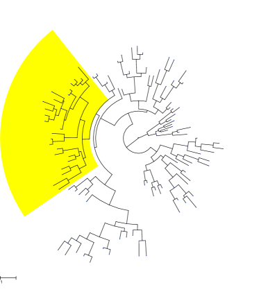
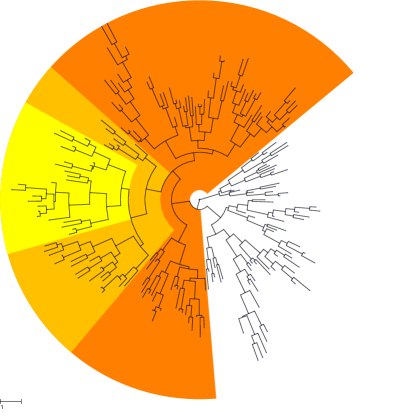
Figure 2: The simulated tree for (left) the first two synthetic studies in section 4.1.1 and 4.1.2, and (right) the third synthetic study in section 4.1.3. Color shading highlights the subtrees affected by branches with jumps.

We evaluate performance using two quantities. The first, which we refer to as “target jump identified”, takes value one when the posterior median estimate of jumps (described in section 3.1) exactly matches the ground truth, i.e. when the target branch and only the target branch is present in the posterior median. The second uses the MCMC samples to compute the Bayes factor of the model with at least one jump to the null model with no jump (see section 3.1 for details). The Bayes factor shows how confident we are of the existence of jumps, with a Bayes factor greater than $10^{2}$ suggests decisive evidence towards the existence of jumps in the tree (see section 3).

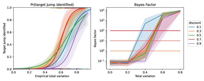
Figure 3: Synthetic study results of section 4.1.1. (left) Estimated probability of identifying the target jump (and the 95% confidence band) versus the empirical total variation. The probability is estimated by fitting a logistic regression to he indicator of identifying the target jump. (right) Bayes factor (mean and the 95% percentile band) versus the total variation. The Bayes factor is truncated at $10^{4}$ to make the plot. The horizontal lines marks the conventional decision boundaries of Bayes factor described in section 3.1.

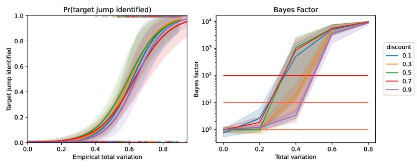
Figure 4: Synthetic study results of section 4.1.1 when the jump rate is known. (left) Estimated probability of identifying the target jump (and the 95% confidence band) versus the empirical total variation. The probability is estimated by fitting a logistic regression to he indicator of identifying the target jump. (right) Bayes factor (mean and the 95% percentile band) versus the total variation. The Bayes factor is truncated at $10^{4}$ to make the plot. The horizontal lines marks the conventional decision boundaries of Bayes factor described in section 3.1.

Figure 3 summarizes the results. with the left panel plotting the probability of identifying the target jump versus the empirical total variation, and the right panel plots the Bayes factor (truncated at $10^{4}$) versus the total variation. For the former, we fit a logistic regression model on the indicator variable, with the empirical total variation as the covariate variable. When the total variation is small (0.2 and 0.4), there is little evidence in the data to support the existence of a jump, and thus, as we expected, both the Bayes factor and the probability of identifying the target is small. For large jump sizes ($\mathrm{TV}=0.8$), the presence of a jump is identified as indicated the large Bayes factor, with ‘Target jump identified’x equal to 1 with high probability, suggesting that there are also few false positives.

Different choices of the discount parameter do not strongly impact the ability to determine the existence of jumps, although a very large discount parameter can harm the ability to correctly locating the jump in the tree. We can see this in the left panel of the figure, where, even when the empirical total variation is large, the probability of identifying the target jump for $d=0.9$ is consistently below other choices of $d$. This is expected, since with a high discount parameter, the model favors many jumps with smaller sizes, resuling in false positives. In practice, we recommend the user to choose a moderate discount parameter, and in the rest of experiments, we fix $d=0.5$.

We further evaluate our algorithm when the jump rate is fixed to have on average one jump in the tree, $\lambda=1/L$. The results are shown in figure 4. Similar to the case when the jump rate is learnt, our algorithm performs well when there is a large change in the distribution before and after the jump. Interestingly, the effect of the discount parameter vanishes in this case, as fixing the jump rate discourages introducing redundant jumps in the model.

4.1.2 Robustness to misspecification of jump rate

In this section, we study how sensitive our approach is to misspecification of the jump rate. Our setup is similar to the previous section (section 4.1.1), except here, we fix the discount parameter to be 0.5. We place an exponential prior on the Poisson jump rate, and investigate performance as we vary its mean between 0.5, 1, 2, 5, or 10 jumps in the tree. In all cases, the ground truth had exactly one branch with jumps.

The results are shown in figure 5, and it is clear that the choice of prior on the rate does not have a significant impact on the probability of identifying the target branch. Thus, when learning the jump rate, our model is very robust to potential misspecification of the prior on jump rate.

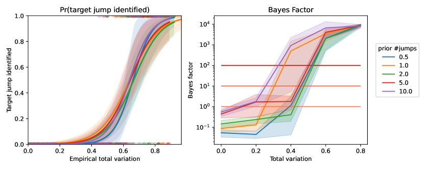
Figure 5: Synthetic study results of section 4.1.2. (left) Estimated probability of identifying the target jump (and the 95% confidence band) versus the empirical total variation. The probability is estimated by fitting a logistic regression to he indicator of identifying the target jump. (right) Bayes factor (mean and the 95 percentile band) versus the total variation. The Bayes factor is truncated at $10^{4}$ to make the plot. The horizontal lines marks the conventional decision boundaries of Bayes factor described in section 3.1.

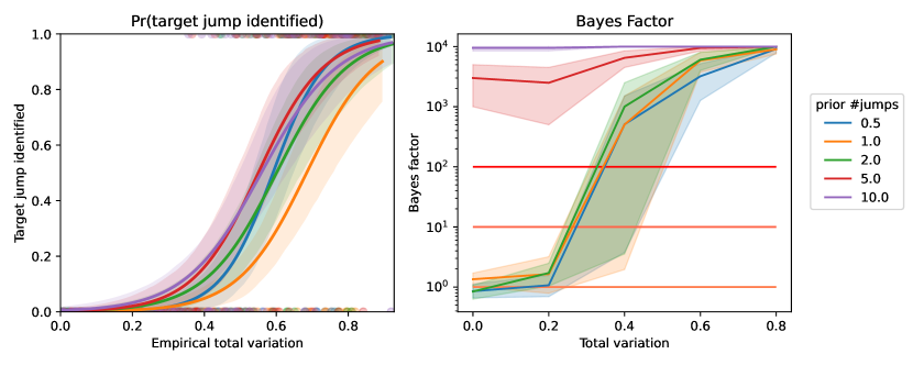
Figure 6: Synthetic study results of section 4.1.2 when the jump rate is known. (left) Estimated probability of identifying the target jump (and the 95% confidence band) versus the empirical total variation. The probability is estimated by fitting a logistic regression to he indicator of identifying the target jump. (right) Bayes factor (mean and the 95 percentile band) versus the total variation. The Bayes factor is truncated at $10^{4}$ to make the plot. The horizontal lines marks the conventional decision boundaries of Bayes factor described in section 3.1.

We also investigate performance when the jump rate is fixed to have also on average 0.5, 1, 2, 5, or 10 number of jumps in the tree, and the result is shown in figure 6. In this case, fixing the jump rate incorrectly has a stronger impact on performance, and the right panel shows that with a high prior number of jumps (5 or 10), the Bayes factor stays very high even when the data provides weak support to the existence of jumps. Taking this into account, we recommend learning the jump rate when there is no strong prior knowledge of the number of jumps in the tree.

4.1.3 Comparison with treeBreaker (Ansari & Didelot, 2016)

Recall that the main difference between the model of treeBreaker and our model is that treeBreaker assumes independence between the distributions before and after a jump while our approach captures the similarity between them by centering the new one on the old one. As a consequence, we expect that for trees with multiple moderate-sized jumps, our model can better leverage the dependency structure between the distributions to outperform treeBreaker. The advantages of our approach are clearest with moderate sized jumps because when the jump size is too small, both approaches will not be able to detect any jumps, and when it is too large, one can to identify the jumps even without considering the dependency structure. Accordingly, we design our study as follows. We first simulated a binary tree with 200 leaves as in the first two synthetic studies, and assigned jumps to three nested branches. Figure 2 (right) shows the simulated tree and the locations of those jumps. The branches are selected to have about 75%, 50% and 25% leaves in the subtrees, so that the four clusters (with different color shadings in figure 2 (right)) of nodes have roughly the same number of observations. The observation distributions of these four clusters are designed to reflect the nested structure of the jumps, with all the three jumps in the “same direction” and of the same size. To be specific, let $p$ denote the total variation between the distributions before and after a jump. The Bernoulli distribution at the root takes 1 with probability $(0.5-1.5p)$, whereas the following ones have probability $(0.5-0.5p)$, $(0.5+0.5p)$, $(0.5+1.5p)$ respectively. With this design, the total variation can take values between 0 and $1/3$, and we simulate 100 datasets for $p$ set to $\{0.05,0.15,0.25\}$ each.

To compare the performance with treeBreaker, we report the average receiver operating characteristic (ROC) curves and area under curve (AUC) for both approaches in figure 7. The ROC curve plots the true positive rate against the false positive rate, and AUC measures the area under a ROC curve. The diagonal line (dotted lines in figure 7) represents random guessing with $\mathrm{AUC}=0.5$. The more a ROC curve bends towards the top left corner, the better the performance is, and as a consequence, high AUC also implies a sound performance of the algorithm. In this study, every run of our algorithm and treeBreaker infers a set of branches with jumps, consisting of the true positives and false positives. Aggregating all the results gives the average ROC curve and the corresponding AUC shown in figure 7. As we expected, when the jump size is relatively small, our approach produces a higher AUC than treeBreaker and performs better. When the total variation is 0.05, the treeBreaker has an average AUC of 0.5 with the ROC curve almost lie exactly on the diagonal line, which suggests that it cannot differentiate branches with jumps from the rest of branches in the tree. Our model performs much better under this situation, as we obtained an average AUC of 0.67. This case is the most difficult one, as the small total variation really cannot provide much evidence to support the existence of jumps. The reason why our approach behaves better in this case is that our model utilizes the shared statistical strength in the dependency structure between the populations, which gives us additional power in detecting jumps. When the jump size increases to (TV=0.15), the difference in AUC of the two models reduces to 0.05, and the ROC curves lie much closer to each other. Although our model still performs better in this case, the edge is not as clear as in the case with a smaller jump size. When the jump size is relatively large (TV = 0.25), our ROC and AUC agree with those of treeBreaker, which suggests that our algorithm has a comparable performance with treeBreaker.

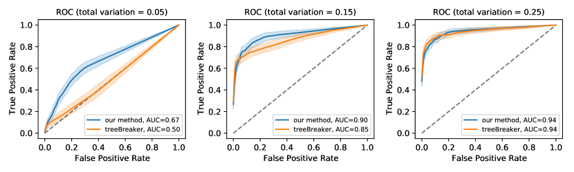
Figure 7: Average ROC curve (with 95 percentile band) and AUC results of section 4.1.3.

4.2 Cytotoxic T-lymphocytes (CTLs) escape mutations in HIV

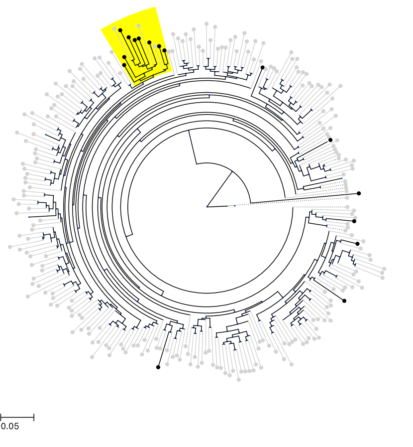
Figure 8: The data and result of the real data study to detect human leukocyte antigen (HLA)-driven evolution of HIV (section 4.2). Dots at leaf nodes represent whether allele B57 exists (black) or not (light grey) in the subject. The Bayes factor we obtained is $+\infty$ suggesting strong evidence towards having jumps in the tree. The color shaded area marks the jump we detected using our algorithm, which is consistent with the findings of Ansari & Didelot (2016). The total runtime of our algorithm is 2098.8s, and it produces ESS/s = 9667.

Human leukocyte antigen (HLA) type I genes are very important to the human immune system, encoding proteins on the surface of human cells which bring epitopes (segments of viral proteins) to the surface when a cell is infected by a virus (Shankarkumar, 2004). Thanks to this functionality, cytotoxic T-lymphocytes (CTLs) (also known as T-cells) can identify the infected cells by recognizing the epitopes and destroy them. HLA-driven mutations of the virus that result in weak binding of epitopes with HLA-encoded proteins can lead to virus escaping the immune response of the host.

In the work of Ansari & Didelot (2016), treeBreaker is applied to the problem of detecting HLA-driven evolution of HIV to determine whether host HLA alleles are randomly distributed on the tips of the virus phylogenetic tree or whether there are clades where the distributions are distinct from each other. The dataset used is from a cohort with 261 subjects (leaf nodes in the tree) published by Carlson et al. (2008). The whole genomes of the viruses are aligned and divided into 10 segments of 1000 nucleotides, and a phylogenetic tree is inferred from each of these alignments. This results in 10 different trees to describe the dependency structure of these 261 populations. One is interested in the distribution of alleles; specifically whether an allele of HLA is present or not forms a binary distribution and observations are available on the leaf nodes of every estimated phylogenetic tree. Ansari & Didelot (2016) studied a number of alleles and identified a jump associated to the distribution of HLA allele B57 in the first phylogenetic tree.

A version of this dataset is available online. Although it slightly differs from the one described in Ansari & Didelot (2016), the difference is too small to significantly affect the final result. We ran our algorithm on this dataset and found that the existence of jumps is strongly supported by the Bayes factor. Figure 8 shows the branch with jumps we detected. This finding agrees with the result in Ansari & Didelot (2016); both methods identify the same clade where 9 out of the 12 hosts have the B57 allele (10 out of 12 in Ansari & Didelot (2016) as their data slightly differs from the one we use), which is a much higher proportion compared to the rest of the tree, where only 7 hosts have allele B57.

4.3 Detecting changes in post-marital residence patterns

Unlike treeBreaker, our implementation also works on more complex scenarios, including the case where the data is not binary. In this study, we apply our approach to detect changepoints in the distribution of post-marital residence patterns within the Uto-Aztecan language family, a dataset where observations take one of four values. The measurements correspond to where newly-wed couple might live after marriage: with the family of the husband (patrilocality), of the wife (matrilocality), of either the husband or the wife (ambilocality) or a new residence separated from their families (neolocality). Moravec et al. (2018) studied the post-marital residence patterns in five different language families. We note that their work focused on how the post-marital residence state transits on individuals, whereas our model focuses on the distributional change in the populations, and therefore, cannot directly compare the two approaches.

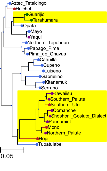
Figure 9: The data and result of the real data study to detect changes in post-marital residence patterns (section 4.3). Dots at the leaf nodes represent the data where the four categories are patrilocality (blue), matrilocality (red), ambilocality (purple) and neolocality (green). We obtain a Bayes factor of 908.76 and locate two branches with jumps as shown with color shading in the tree. The runtime of our algorithm is 208.8s, and it produces ESS/s = 10.

We obtained the dataset directly from the authors and only explore the Uto-Aztecan language family, the smallest among the five. This language family forms a language tree with node representing language communities. There are 26 communities at leaf of the tree, and the primary social norm of post-marital residence is obtained for each of them. Running our algorithm on this dataset produces a Bayes factor of 908.76 which strongly suggests changes of distributions happening in the tree. In total, we locate two branches with jumps in the tree, and figure 9 shows the data and our results. Professor Murray Cox, a domain expert, helped us gain insight into the result. For the cluster at the root (above both jumps), new couples in the population prefer to reside with the husband (patrilocality). The first jump at the top portion of the tree creates a cluster at the subtree of Guarijio and Tarahumara, where new couples tend to seek new residence (neolocality). These two languages are spoken in a region with quite poor soil, so newly married couples have to move to a new location to find productive farming land. The second jump at the bottom portion of the tree instead switches towards a distribution that strongly favors matrilocality and ambilocality. This is probably due to the change of practices result from transitioning into more desert-plains environment.

5 Discussions

Our approach models the evolution of distributions on a phylogenetic tree, and it can be viewed as an analogue to a pure jump model on individual trait evolution. However, it also connects to the continuous random walk model on individual trait evolution. With a large discount parameter, samples from the PYP has smaller variance, which means that the generated distribution will be closer to the center. This behavior mimics the effect of having jumps with a smaller step size. With multiple small jumps on each branch along the tree, the pure jump model will have the ability to model gradual evolution as well as rapid evolution at the same time. Therefore, our proposed method could be regarded as the bridge between a continuous process model and a pure jump model of distribution evolution on the tree.

There are a number of potential future directions. A natural extension to develop our model to work with continuous distributions. Carrying this out is relatively straightforward, and requires framing each node density $G_{i}$ as a mixture model specified by a Pitman-Yor prior. Another direction is to extend the dependency structure from a tree to a network so that it finds a much wider applications in real-world problems. As for the theoretical direction, we are interested in the asymptotic behavior of the model, as well as assessing the mixing of the MCMC. Also, finding new applications of our approach, especially beyond the scope of evolution trees, can be very exciting.

References

- (1)
- Andrieu et al. (2010) Andrieu, C., Doucet, A. & Holenstein, R. (2010), ‘Particle markov chain monte carlo methods’, Journal of the Royal Statistical Society: Series B (Statistical Methodology) 72(3), 269–342.
- Andrieu et al. (2009) Andrieu, C., Roberts, G. O. et al. (2009), ‘The pseudo-marginal approach for efficient monte carlo computations’, The Annals of Statistics 37(2), 697–725.
- Ansari & Didelot (2016) Ansari, M. A. & Didelot, X. (2016), ‘Bayesian inference of the evolution of a phenotype distribution on a phylogenetic tree’, Genetics 204(1), 89–98.
- Bianchini et al. (2018) Bianchini, I., Guglielmi, A., Quintana, F. A. et al. (2018), ‘Determinantal point process mixtures via spectral density approach’, Bayesian Analysis .
- Brawand et al. (2011) Brawand, D., Soumillon, M., Necsulea, A., Julien, P., Csárdi, G., Harrigan, P., Weier, M., Liechti, A., Aximu-Petri, A., Kircher, M. et al. (2011), ‘The evolution of gene expression levels in mammalian organs’, Nature 478(7369), 343.
- Carlson et al. (2008) Carlson, J. M., Brumme, Z. L., Rousseau, C. M., Brumme, C. J., Matthews, P., Kadie, C., Mullins, J. I., Walker, B. D., Harrigan, P. R., Goulder, P. J. et al. (2008), ‘Phylogenetic dependency networks: inferring patterns of ctl escape and codon covariation in hiv-1 gag’, PLoS computational biology 4(11), e1000225.
- Duchen et al. (2017) Duchen, P., Leuenberger, C., Szilágyi, S. M., Harmon, L., Eastman, J., Schweizer, M. & Wegmann, D. (2017), ‘Inference of evolutionary jumps in large phylogenies using lévy processes’, Systematic biology 66(6), 950–963.
-
Felsenstein (1985)
Felsenstein, J. (1985), ‘Phylogenies and the
comparative method’, The American Naturalist 125(1), 1–15.
http://www.jstor.org/stable/2461605 - Felsenstein (2008) Felsenstein, J. (2008), ‘Comparative methods with sampling error and within-species variation: contrasts revisited and revised’, The American Naturalist 171(6), 713–725.
- Ferguson (1973) Ferguson, T. S. (1973), ‘A bayesian analysis of some nonparametric problems’, The annals of statistics pp. 209–230.
- Freckleton et al. (2002) Freckleton, R. P., Harvey, P. H. & Pagel, M. (2002), ‘Phylogenetic analysis and comparative data: a test and review of evidence’, The American Naturalist 160(6), 712–726.
- Ives et al. (2007) Ives, A. R., Midford, P. E. & Garland Jr, T. (2007), ‘Within-species variation and measurement error in phylogenetic comparative methods’, Systematic biology 56(2), 252–270.
- Jeffreys (1961) Jeffreys, H. (1961), The theory of probability, Oxford University Press.
- Kass & Raftery (1995) Kass, R. E. & Raftery, A. E. (1995), ‘Bayes factors’, Journal of the american statistical association 90(430), 773–795.
- Kostikova et al. (2016) Kostikova, A., Silvestro, D., Pearman, P. B. & Salamin, N. (2016), ‘Bridging inter-and intraspecific trait evolution with a hierarchical bayesian approach’, Systematic biology 65(3), 417–431.
- Landis et al. (2012) Landis, M. J., Schraiber, J. G. & Liang, M. (2012), ‘Phylogenetic analysis using lévy processes: finding jumps in the evolution of continuous traits’, Systematic biology 62(2), 193–204.
- Landis & Schraiber (2017) Landis, M. & Schraiber, J. G. (2017), ‘Punctuated evolution shaped modern vertebrate diversity’, bioRxiv p. 151175.
- Lau & Green (2007) Lau, J. W. & Green, P. J. (2007), ‘Bayesian model-based clustering procedures’, Journal of Computational and Graphical Statistics 16(3), 526–558.
- Moravec et al. (2018) Moravec, J. C., Atkinson, Q., Bowern, C., Greenhill, S. J., Jordan, F. M., Ross, R. M., Gray, R., Marsland, S. & Cox, M. P. (2018), ‘Post-marital residence patterns show lineage-specific evolution’, Evolution and Human Behavior 39(6), 594–601.
- Paradis & Schliep (2019) Paradis, E. & Schliep, K. (2019), ‘Ape 5.0: an environment for modern phylogenetics and evolutionary analyses in R’, Bioinformatics 35, 526–528.
- Pitman & Yor (1997) Pitman, J. & Yor, M. (1997), ‘The two-parameter poisson-dirichlet distribution derived from a stable subordinator’, The Annals of Probability pp. 855–900.
-
Plummer et al. (2006)
Plummer, M., Best, N., Cowles, K. & Vines, K. (2006), ‘CODA: convergence diagnosis and output analysis for
MCMC’, R News 6(1), 7–11.
https://journal.r-project.org/archive/ - Revell & Graham Reynolds (2012) Revell, L. J. & Graham Reynolds, R. (2012), ‘A new bayesian method for fitting evolutionary models to comparative data with intraspecific variation’, Evolution: International Journal of Organic Evolution 66(9), 2697–2707.
- Shankarkumar (2004) Shankarkumar, U. (2004), ‘The human leukocyte antigen (hla) system’, International Journal of Human Genetics 4(2), 91–103.
- Teh (2006) Teh, Y. W. (2006), A hierarchical bayesian language model based on pitman-yor processes, in ‘Proceedings of the 21st International Conference on Computational Linguistics and the 44th annual meeting of the Association for Computational Linguistics’, Association for Computational Linguistics, pp. 985–992.
- Teh et al. (2006) Teh, Y. W., Jordan, M. I., Beal, M. J. & Blei, D. M. (2006), ‘Hierarchical dirichlet processes’, Journal of the american statistical association 101(476), 1566–1581.