The Provable Benefits of Unsupervised Data Sharing for Offline Reinforcement Learning

Abstract

Self-supervised methods have become crucial for advancing deep learning by leveraging data itself to reduce the need for expensive annotations. However, the question of how to conduct self-supervised offline reinforcement learning (RL) in a principled way remains unclear. In this paper, we address this issue by investigating the theoretical benefits of utilizing reward-free data in linear Markov Decision Processes (MDPs) within a semi-supervised setting. Further, we propose a novel, Provable Data Sharing algorithm (PDS) to utilize such reward-free data for offline RL. PDS uses additional penalties on the reward function learned from labeled data to prevent overestimation, ensuring a conservative algorithm. Our results on various offline RL tasks demonstrate that PDS significantly improves the performance of offline RL algorithms with reward-free data. Overall, our work provides a promising approach to leveraging the benefits of unlabeled data in offline RL while maintaining theoretical guarantees. We believe our findings will contribute to developing more robust self-supervised RL methods.

1 Introduction

Offline reinforcement learning (RL) is a promising framework for learning sequential policies with pre-collected datasets. It is highly preferred in many real-world problems where active data collection and exploration is expensive, unsafe, or infeasible (Swaminathan & Joachims, 2015; Shalev-Shwartz et al., 2016; Singh et al., 2020). However, labeling large datasets with rewards can be costly and require significant human effort (Singh et al., 2019; Wirth et al., 2017). In contrast, unlabeled data can be cheap and abundant, making self-supervised learning with unlabeled data an attractive alternative. While self-supervised methods have achieved great success in computer vision and natural language processing tasks (Brown et al., 2020; Devlin et al., 2018; Chen et al., 2020), their potential benefits in offline RL are less explored.

Several prior works (Ho & Ermon, 2016; Reddy et al., 2019; Kostrikov et al., 2019) have explored demonstration-based approaches to eliminate the need for reward annotations, but these approaches require samples to be near-optimal. Another line of work focuses on data sharing from different datasets (Kalashnikov et al., 2021; Yu et al., 2021a). Still, it assumes that the dataset can be relabeled with oracle reward functions for the target task. These settings can be unrealistic in real-world problems where expert trajectories and reward labeling are expensive.

Incorporating reward-free datasets into offline RL is important but challenging due to the sequential and dynamic nature of RL problems. Prior work (Yu et al., 2022) has shown that learning to predict rewards can be difficult, and simply setting the reward to zero can achieve good results. However, it’s unclear how reward-prediction methods affect performance and whether reward-free data can provably benefit offline RL. This naturally leads to the following question:

How can we leverage reward-free data to improve the performance of offline RL algorithms
in a principled way?

To answer this question, we conduct a theoretical analysis of the benefits of utilizing unlabeled data in linear MDPs. Our analysis reveals that although unlabeled data can provide information about the dynamics of the MDP, it cannot reduce the uncertainty over reward functions. Based on this insight, we propose a model-free method named Provable Data Sharing (PDS), which adds uncertainty penalties to the learned reward functions to maintain a conservative algorithm. By doing so, PDS can effectively leverage the benefits of unlabeled data for offline RL while ensuring theoretical guarantees.

We demonstrate that PDS can cooperate with model-free offline methods while being simple and efficient. We conduct extensive experiments on various environments, including single-task domains like MuJoCo (Todorov et al., 2012) and Kitchen (Gupta et al., 2019), as well as multi-task domains like AntMaze and Meta-World (Yu et al., 2020a). The results show that PDS improves significantly over previous methods like UDS (Yu et al., 2022) and naive reward prediction methods.

Our main contribution is the Provable Data Sharing (PDS) algorithm, a novel method for utilizing unsupervised data in offline RL that provides theoretical guarantees. PDS adds uncertainty penalties to the learned reward functions and can be easily integrated with existing offline RL algorithms. Our experimental results demonstrate that PDS can achieve superior performance on various locomotion, navigation, and manipulation tasks. Overall, our work provides a promising approach to leveraging the benefits of unlabeled data in offline RL while maintaining theoretical guarantees and contributing to the development of more robust self-supervised RL methods.

2 Related Work

Offline Reinforcement Learning

Current offline RL methods (Levine et al., 2020) can be roughly divided into policy constraint-based, uncertainty estimation-based, and model-based approaches. Policy constraint methods aim to keep the policy close to the behavior under a probabilistic distance (Siegel et al., 2020; Yang et al., 2021; Kumar et al., 2020; Fujimoto & Gu, 2021; Yang et al., 2022; Fujimoto et al., 2019; Hu et al., 2022; Kostrikov et al., 2021; Ma et al., 2021; Wang et al., 2021). Uncertainty estimation-based methods attempt to consider the Q-value prediction’s confidence using dropout or ensemble techniques (An et al., 2021; Wu et al., 2021). Last, model-based methods incorporates the uncertainty in the model space for conservative offline learning (Yu et al., 2020b; 2021b; Kidambi et al., 2020).

Offline Data Sharing

Prior works have demonstrated that data sharing across tasks can be beneficial by designing sophisticated data-sharing protocols (Yu et al., 2021a). For example, previous studies have explored developing data sharing strategies by human effort (Kalashnikov et al., 2021), inverse RL (Reddy et al., 2019; Li et al., 2020), and estimated Q-values (Yu et al., 2021a). However, these data sharing works must assume the dataset can be relabeled with oracle rewards for the target task, which is a strong assumption since the high cost of reward labeling. Therefore, effectively incorporating the unlabeled data into the offline RL algorithms is essential. To solve this issue, some recent work (Yu et al., 2022) proposes simply applying zero rewards to unlabeled data. In this work, we propose a principle way to leverage unlabeled data without the strong assumption of reward relabeling.

Reward Prediction

It is widely observed that reward shaping and intrinsic rewards can accelerate learning in online RL (Mataric, 1994; Ng et al., 1999; Wu & Tian, 2017; Song et al., 2019; Guo et al., 2016; Abel et al., 2021). There are also extensive works that studies automatically designing reward functions using inverse RL (Ng et al., 2000; Fu et al., 2017). However, there is less attention on the offline setting where online interaction is not allowed and the trajectories may not be optimal.

3 Preliminaries

3.1 Linear MDPs and Performance Metric

We consider infinite-horizon discounted Markov Decision Processes (MDPs), defined by the tuple $(\mathcal{S},\mathcal{A},\mathcal{P},r,\gamma),$ with state space $\mathcal{S}$, action space $\mathcal{A}$, discount factor $\gamma\in[0,1)$, transition function $\mathcal{P}:\mathcal{S}\times\mathcal{A}\rightarrow\Delta(\mathcal{S})$, and reward function $r:\mathcal{S}\times\mathcal{A}\rightarrow[0,r_{\text{max}}]$. To make things more concrete, we consider the linear MDP (Yang & Wang, 2019; Jin et al., 2020) as follows, where the transition kernel and expected reward function are linear with respect to a feature map.

Definition 3.1 (Linear MDP).

We say an episodic MDP $({\mathcal{S}},\mathcal{A},\mathcal{P},r,\gamma)$ is a linear MDP with known feature map $\phi:{\mathcal{S}}\times\mathcal{A}\to\mathbb{R}^{d}$ if there exist unknown measures $\mu=(\mu_{1},\ldots,\mu_{d})$ over ${\mathcal{S}}$ and an unknown vector $\theta\in\mathbb{R}^{d}$ such that

$$\mathcal{P}(s^{\prime}{\,|\,}s,a)=\langle\phi(s,a),\mu(s^{\prime})\rangle,\quad r(s,a)=\langle\phi(s,a),\theta\rangle$$ (1)

for all $(s,a,s^{\prime})\in{\mathcal{S}}\times\mathcal{A}\times{\mathcal{S}}$. And we assume $\|\phi(s,a)\|_{2}\leq 1$ for all $(s,a,s^{\prime})\in{\mathcal{S}}\times\mathcal{A}\times{\mathcal{S}}$ and $\max\{\|\mu({\mathcal{S}})\|_{2},\|\theta\|_{2}\}\leq\sqrt{d}$, where $\|\mu({\mathcal{S}})\|\equiv\int_{{\mathcal{S}}}\|\mu(s)\|ds$.

A policy $\pi:{\mathcal{S}}\rightarrow\Delta{(\mathcal{A})}$ specifies a decision-making strategy in which the agent chooses actions adaptively based on the current state, i.e., $a_{t}\sim\pi(\cdot{\,|\,}s_{t})$. The value function $V^{\pi}:{\mathcal{S}}\rightarrow\mathbb{R}$ and the action-value function (Q-function) $Q^{\pi}:{\mathcal{S}}\times\mathcal{A}\to\mathbb{R}$ are defined as

$$V^{\pi}(s)=\mathbb{E}_{\pi}\Big{[}\sum_{t=0}^{\infty}\gamma^{t}r(s_{t},a_{t})\,\Big{|}\,s_{0}=s\Big{]},\quad Q^{\pi}(s,a)=\mathbb{E}_{\pi}\Big{[}\sum_{t=0}^{\infty}\gamma^{t}r(s_{t},a_{t})\,\Big{|}\,s_{0}=s,a_{0}=a\Big{]}.$$ (2)

where the expectation is with respect to the trajectory $\tau$ induced by policy $\pi$.

We define the Bellman operator as

$$(\mathbb{B}f)(s,a)=\mathbb{E}_{s^{\prime}\sim p(\cdot|s,a)}\bigl{[}r(s,a)+\gamma f(s^{\prime})\bigr{]}.$$ (3)

We use $\pi^{*}$, $Q^{*}$, and $V^{*}$ to denote the optimal policy, optimal Q-function, and optimal value function, respectively. We have the Bellman optimality equation

$$V^{*}(s)=\max_{a\in\mathcal{A}}Q^{*}(s,a),\quad Q^{*}(s,a)=(\mathbb{B}V^{*})(s,a).$$ (4)

Meanwhile, the optimal policy $\pi^{*}$ satisfies

$$\pi^{*}(\cdot{\,|\,}s)=\mathop{\mathrm{argmax}}_{\pi}\langle Q^{*}(s,\cdot),\pi(\cdot{\,|\,}s)\rangle_{\mathcal{A}},\quad V^{*}(s)=\langle Q^{*}(s,\cdot),\pi^{*}(\cdot{\,|\,}s)\rangle_{\mathcal{A}},$$

where the maximum is taken over all functions mapping from ${\mathcal{S}}$ to distributions over $\mathcal{A}$. We aim to learn a policy that maximizes the expected cumulative reward. Correspondingly, we define the performance metric as

$$\text{SubOpt}(\pi,s)=V^{\pi^{*}}(s)-V^{\pi}(s).$$ (5)

3.2 Provable Offline Algorithms

In this section, we consider pessimistic value iteration (PEVI; Jin et al., 2021) as the backbone algorithm, described in Algorithm 2. It is a representative model-free offline algorithm with theoretical guarantees. PEVI uses negative bonus $\Gamma(\cdot,\cdot)$ over standard $Q$-value estimation $\widehat{Q}(\cdot,\cdot)=(\widehat{\mathbb{B}}\widehat{V})(\cdot)$ to reduce potential bias due to finite data, where $\widehat{\mathbb{B}}$ is some empirical estimation of $\mathbb{B}$ from dataset $\mathcal{D}$. Please refer to Appendix A.1 for more details of the PEVI algorithm.

We use the following notion of $\xi$-uncertainty quantifier as follows to formalize the idea of pessimism.

Definition 3.2 ($\xi$-Uncertainty Quantifier).

We say $\Gamma:{\mathcal{S}}\times\mathcal{A}\to\mathbb{R}$ is a $\xi$-uncertainty quantifier for $\widehat{\mathbb{B}}$ and $\widehat{V}$ if with probability $1-\xi$, for all $(s,a)\in{\mathcal{S}}\times\mathcal{A}$,

$$\big{|}(\widehat{\mathbb{B}}\widehat{V})(s,a)-(\mathbb{B}\widehat{V})(s,a)\big{|}\leq\Gamma(s,a).$$ (6)

3.3 Unsupervised Data Sharing

We consider unsupervised data sharing in offline reinforcement learning. We first characterize the quality of the dataset with the notion of coverage coefficient (Uehara & Sun, 2021), defined as below.

Definition 3.3.

The coverage coefficient $C^{\dagger}$ of a dataset $\mathcal{D}=\{(s_{\tau},a_{\tau},r_{\tau})\}_{\tau=1}^{N}$ is defined as

$$C^{\dagger}=\sup_{C}\left\{\frac{1}{N}\cdot\sum_{\tau=1}^{N}{\phi(s_{\tau},a_{\tau})\phi(s_{\tau},a_{\tau})^{\top}}\succeq C\cdot\mathbb{E}_{\pi^{*}}\bigl{[}\phi(s_{t},a_{t})\phi(s_{t},a_{t})^{\top}\,\big{|}\,s_{0}=s\bigr{]},\forall s\in{\mathcal{S}}\right\},$$

The coverage coefficient $C^{\dagger}$ is common in offline RL literature (Uehara & Sun, 2021; Jin et al., 2021; Rashidinejad et al., 2021), which represents the maximum ratio between the density of empirical state-action distribution and the density induced from the optimal policy. Intuitively, it represents the quality of the dataset. For example, the expert dataset has a high coverage ratio while the random dataset may have a low ratio.

We denote $\mathcal{D}_{0}$ as the origin labeled dataset, with coverage coefficient $C_{0}^{\dagger}$ and size $N_{0}$. And we denote the unlabeled dataset as $\mathcal{D}_{1}$, with coverage coefficient $C_{1}^{\dagger}$ and size $N_{1}$. Note that it is possible that the unlabeled data comes from multiple sources, such as multi-task settings, and we still use $\mathcal{D}_{1}$ to represent the combined dataset $\cup_{i=1}^{M}\mathcal{D}_{i}$ from $M$ tasks for simplicity.

4 Provable Unsupervised Data Sharing

How can we leverage reward-free data for offline RL? A naive approach is to learn the reward function from labeled data via the following regression

$$\widehat{\theta}=\mathop{\mathrm{argmin}}_{\theta}\sum_{\tau=1}^{N_{0}}{\left(f_{\theta}(s_{\tau},a_{\tau})-r_{\tau}\right)^{2}}+\frac{\nu}{2}\|\theta\|^{2}_{2},$$ (7)

where $f_{\theta}(s_{\tau},a_{\tau})=\phi(s_{\tau},a_{\tau})^{\top}\theta$ in linear MDPs. Then we can use this learned reward function to label unsupervised data. However, this approach can lead to suboptimal performance due to overestimation of the predicted reward $r_{\widehat{\theta}}$ (Yu et al., 2022), which undermines the pessimism in offline algorithms.

To address this issue, we propose a data-sharing algorithm called Provable Data Sharing (PDS). We start by analyzing the uncertainty in learned reward functions and add penalties for such uncertainty to leverage unlabeled data. In Section 4.2, we show that PDS has a provable performance bound consisting of two parts: the offline error, which is tightened compared to no data sharing due to additional data, and the error from reward bias. The performance bound of PDS is provably better than no data sharing as long as the unlabeled dataset has mediocre size or quality. We also extend our algorithm in linear MDPs to general settings in Section 4.3 and propose using ensembles for reward uncertainty estimation. We demonstrate the effectiveness of PDS by integrating it with IQL (Kostrikov et al., 2021), and present Algorithm 3, which is simple and can be easily integrated with other model-free offline algorithms.

4.1 Provable Data Sharing

To address the issue of potential overestimation of predicted rewards, we first analyze the uncertainty in learned reward functions. In the context of linear MDPs, the reward function can be learned via linear regression, and the uncertainty of the parameters is characterized by the elliptical confidence region, as shown in Lemma 4.1. This confidence region is important as it allows us to give a more accurate estimation of the reward function while keeping the overall algorithm pessimistic.

Lemma 4.1 ( Abbasi-Yadkori et al. (2011)).

Let $\alpha=\sqrt{\nu}+r_{\text{\rm max}}\cdot\sqrt{2\log{\frac{1}{\delta}}+d\log{(1+\frac{N_{0}}{\nu d})}},\Lambda=\nu I+\sum_{\tau=1}^{N_{0}}{\phi(s_{\tau},a_{\tau})\phi(s_{\tau},a_{\tau})^{\top}}$,

$$\quad\mathcal{C}(\delta)=\left\{\theta\in\mathbb{R}^{d}\mid\|\theta-\widehat{\theta}\|_{\Lambda}\leq\alpha\right\},$$ (8)

where $\widehat{\theta}$ is the minimizer in Equation (7), then we have $\mathcal{P}(\theta^{\star}\in\mathcal{C}(\delta))\geq 1-\delta$, where $\theta^{\star}$ is the true parameter for the reward function.

Proof.

Please refer to Theorem 2 in Abbasi-Yadkori et al. (2011) for detailed proof. ∎

Lemma 4.1 provides a useful insight: the uncertainty of the learned reward function in linear MDPs only depends on the quality and size of labeled data. Based on this insight, we propose a two-phase algorithm that guarantees a provable performance bound, as shown in Theorem 4.3. The simple reward prediction method can compromise the pessimistic estimation of the algorithm, while UDS may result in a reward bias that is too large. Our algorithm consists of two phases: in the first phase, we construct a pessimistic reward estimator that finds the reward function in the confidence set that leads to the lowest optimal value. In the second phase, we conduct standard offline RL with the given pessimistic reward function.

To solve the challenge of finding the best parameter in the confidence set, which is a bi-level optimization problem, we propose using a simpler method that maintains the pessimistic property of the offline algorithms. This method involves using a pessimistic estimation, which allows us to keep the algorithm pessimistic while avoiding the computational challenges of the bi-level optimization problem. Formally,

$$\widehat{r}(s,a)=\max\left\{\phi(s,a)^{\top}\widehat{\theta}-\alpha\sqrt{\phi(s,a)^{\top}\Lambda^{-1}\phi(s,a)},0\right\},$$ (9)

where $\Lambda=\nu I+\sum_{\tau=1}^{N_{0}}{\phi(s_{\tau},a_{\tau})\phi(s_{\tau},a_{\tau})^{\top}}$.

We adopt the pessimistic estimation in Equation (9) because it provides a lower bound for reward functions in the confidence set $\mathcal{C}(\delta)$, as guaranteed by the following lemma derived from Cauchy-Schwartz inequalities.

Lemma 4.2.

For any $\theta\in\mathcal{C}(\delta)$,

$$\left|\phi(s,a)^{\top}\theta-\phi(s,a)^{\top}\widehat{\theta}\right|\leq\alpha\sqrt{\phi(s,a)^{\top}\Lambda^{-1}\phi(s,a)}.$$ (10)

When labeled data is scarce or there is a significant distributional shift between the labeled and unlabeled data, Equation (9) degenerates to 0, which is equivalent to the UDS algorithm (Yu et al., 2022).

Algorithm 1 Provable Data Sharing, Linear MDP

1:  Require: Labeled dataset $\mathcal{D}_{0}=\{(s_{\tau},a_{\tau},r_{\tau})\}_{\tau=1}^{N_{0}}$, unlabeled dataset $\mathcal{D}_{1}=\{(s_{\tau},a_{\tau})\}_{\tau=1}^{N_{1}}$.

2:  Require: Confidence parameter $\alpha,\beta,\delta$.

3:  Learn the reward function $\widehat{\theta}$ from $\mathcal{D}_{0}$ using Equation (7)

4:  Construct the confidence set $\mathcal{C}(\delta)$ using Equation (8).

5:  Construct the pessimistic reward over the confidence set

$$\widetilde{\theta}\leftarrow\mathop{\mathrm{argmin}}_{\theta\in\mathcal{C}(\delta)}\widehat{V}_{\theta},$$ (11)

where $\widehat{V}_{\theta}$ is the estimated value function from Algorithm 2 and dataset $\mathcal{D}_{0}\cup\mathcal{D}_{1}$ with reward relabeled with parameter $\theta$.

6:  Annotate the reward in $\mathcal{D}_{0}\cup\mathcal{D}_{1}$ with parameter $\widetilde{\theta}$.

7:  Learn the policy from the annotated dataset $\mathcal{D}_{0}\cup\mathcal{D}_{1}$ using Algorithm 2

$$\widehat{V},\widehat{\pi}\leftarrow\text{PEVI}(\mathcal{D}_{0}\cup\mathcal{D}_{1}).$$ (12)

8:  Return $\widehat{\pi}$

4.2 Theoretical Analysis

The following subsection analyzes how the provable data-sharing (PDS) algorithm can enhance the performance bound by leveraging unlabeled data. To be specific, we present the following theorem.

Theorem 4.3 (Performance Bound for PDS).

Suppose the dataset $\mathcal{D}_{0},\mathcal{D}_{1}$ have positive coverage coefficients $C^{\dagger}_{0},C^{\dagger}_{1}$, and the underlying MDP is a linear MDP. In Algorithm 1, we set

$$\lambda=1,\nu=1,\alpha=2\sqrt{d\zeta_{2}}\cdot r_{\text{\rm max}},\beta=\frac{cd\sqrt{\zeta_{1}}}{1-\gamma}\cdot r_{\text{\rm max}},\zeta_{1}=\log{\left(\frac{4d(N_{0}+N_{1})}{(1-\gamma)\delta}\right)},\zeta_{2}=\log{\left(\frac{2dN_{0}}{\delta}\right)},$$

where $c>0$ is an absolute constant and $\delta\in(0,1)$ is the confidence parameter. Then with probability $1-2\delta$, the policy $\widehat{\pi}$ generated by PDS satisfies for all $s\in{\mathcal{S}}$,

$$\text{\rm SubOpt}\big{(}\widehat{\pi};s\big{)}\leq\frac{2cr_{\text{\rm max}}}{(1-\gamma)^{2}}\sqrt{\frac{d^{3}\zeta_{1}}{N_{0}C^{\dagger}_{0}+N_{1}C^{\dagger}_{1}}}+\frac{4r_{\text{\rm max}}}{1-\gamma}\sqrt{\frac{d^{2}\zeta_{2}}{N_{0}C_{0}^{\dagger}}}.$$

Proof.

Please refer to Appendix B for detailed proof. ∎

The performance bound of PDS is composed of two terms. The first is the offline error, which is inherited from offline algorithms. This bound is improved when additional unlabeled data with size $N_{1}$ and coverage $C_{1}^{\dagger}$ is available. The second term is the reward bias, which arises due to uncertainties in the rewards. Notably, this term is equivalent to the performance bound of a linear bandit with rewards in the range $[0,r_{\text{\rm max}}/(1-\gamma)]$. As the number of unlabeled data approaches infinity, the uncertainty of the dynamics decreases to zero, and the RL problem becomes a linear bandit problem. The theorem demonstrates that PDS outperforms UDS, which suffers from a constant reward bias, and naive reward prediction methods, which lack pessimism and therefore do not offer such guarantees. Moreover, we demonstrate the tightness of the bound by constructing an “adversarial” dataset that matches the bound’s suboptimality (see Appendix F).

To better understand the benefits of unlabeled data, we define the suboptimality bound ratio (SBR) of an offline algorithm $\mathcal{A}$ as the ratio of the suboptimality bound obtained by the policy learned with additional unlabeled data to the suboptimality bound of the policy learned using labeled data alone. Mathematically, the SBR of $\mathcal{A}$ is given by:

$$\text{\rm SBR}(\mathcal{A})=\frac{\overline{\text{\rm SubOpt}}\big{(}\widehat{\pi}{\mathcal{A}}(\mathcal{D}_{0},\mathcal{D}_{1})\big{)}}{\overline{\text{\rm SubOpt}}\big{(}\widehat{\pi}{\mathcal{A}}(\mathcal{D}_{0},\varnothing)\big{)}},$$ (13)

where $\overline{\text{\rm SubOpt}}$ is the tight upper bound on suboptimality. The SBR provides a measure of the benefit of unlabeled data to the offline algorithm, with a smaller SBR indicating a greater benefit from the unlabeled data. Applying this definition to PDS, we obtain the following corollary.

Corollary 4.4 (Informal).

The SBR of PDS satisfies

$$\text{\rm SBR}\approx\underbrace{\sqrt{\frac{N_{0}C^{\dagger}_{0}}{N_{0}C^{\dagger}_{0}+N_{1}C^{\dagger}_{1}}}}_{\text{\rm finite sample term}}+\underbrace{\frac{2(1-\gamma)}{c\sqrt{d}}}_{\text{\rm asymptotic term}},$$ (14)

where $c$ is the constant in Theorem 4.3 and we ignore the logarithmic factors.

When does unlabeled data improve the performance of offline algorithms?

Corollary 4.4 allows us to analyze the relative performance of PDS under different conditions. The first term of the bound depends on the qualities and amounts of both labeled and unlabeled datasets. If the unlabeled dataset has a mediocre number of samples or data quality, the first term will be sufficiently small. The second term affects the asymptotic performance when the unlabeled data approaches infinity, and it depends on the discount factor and the dimension of the problem. PDS improves over no data-sharing algorithms asymptotically in larger problems or longer horizons. For a more detailed discussion, please refer to Appendix E.

4.3 Practical Implementation

This subsection outlines the practical implementation of PDS in general MDPs. We employ $L$ ensembles ${\theta_{1},\ldots,\theta_{L}}$ to estimate uncertainty, which are learned using Equation (7). To estimate pessimistic rewards, we use the following pessimistic estimation:

$$\widehat{r}(s,a)=\max\left\{\mu(s,a)-k\sigma(s,a),0\right\},$$ (15)

where $\mu(s,a)=\frac{1}{L}\sum_{i=1}^{L}f_{\theta_{i}}(s,a),\sigma(s,a)=\sqrt{\frac{1}{L}\sum_{i=1}^{L}(f_{\theta_{i}}(s,a)-\mu(s,a))^{2}}$ are the mean and standard deviation, respectively. Here, $k$ is a hyperparameter used to control the amount of pessimism. We can also use the minimum over $L$ ensembles for the pessimistic estimation, which is linked to Equation (15) following An et al. (2021); Royston (1982) as shown in Equation (16):

$$\mathbb{E}{\left[\min_{j=1,\ldots,L}f_{\theta_{j}}(s,a)\right]}\approx\mu(s,a)-\Phi^{-1}\left(\frac{L-\frac{\pi}{8}}{L-\frac{\pi}{4}+1}\right)\sigma(s,a),$$ (16)

where $\Phi$ is the CDF of the standard Gaussian distribution.

The appropriate value of $k$ for each domain can be difficult to determine. To address this issue, we observe that the amount of pessimism required for different domains is proportional to the difference in mean rewards between labeled and unlabeled data. Leveraging this insight, we propose a simple and efficient automatic mechanism for adjusting the value of the $k$ parameter. Specifically, we suggest a method that adjusts $k$ based on the difference in mean rewards, as given by Equation (17):

$$\widehat{r}(s,a) =\max\left\{\min_{j=1,\ldots,L}f_{\theta_{j}}(s,a)-k\sigma(s,a),0\right\},$$

$$\text{where}\quad k=a\cdot\frac{\max({\mu-\widehat{\mu}},0)}{{|\mu|+\epsilon}}.$$ (17)

where $\mu=\frac{1}{N_{0}}\sum_{i=1}^{N_{0}}\mu(s_{i},a_{i}),\widehat{\mu}=\frac{1}{N_{1}}\sum_{i=1}^{N_{1}}\widehat{\mu}(s_{i},a_{i})$ are the mean reward of labeled and (predicted) unlabeled data, respectively. We use $a=25$ and $L=10$ in all experiments.

Then we can plug in any model-free offline algorithms. Here we use IQL (Kostrikov et al., 2021) as the backbone offline algorithm, but we emphasize that it can be easily integrated with other model-free algorithms. The details of our algorithm is summarized in Algorithm 3 in Appendix A.2.

5 Experiments

In this section, we aim to evaluate the effectiveness of pessimistic reward estimation and answer the following questions: (1) How does PDS perform compared to the naive reward prediction and unlabeled data sharing (UDS) methods in single locomotion and manipulation tasks? (2) How does PDS behave in multi-task offline RL settings compared to baselines? (3) What makes PDS effective?

Algorithm	door-open	door-close	drawer-open	drawer-close	average
UDS	16.2$\pm$12.1	0.0$\pm$0.0	30.4$\pm$60.4	182.2$\pm$0.4	57.2$\pm$30.8
Rew Pred	26.4$\pm$12.9	110.8$\pm$14.3	102.6$\pm$40.2	182.2$\pm$0.4	105.5$\pm$22.3
PDS	25.5$\pm$15.5	114.3$\pm$1.8	153.8$\pm$0.4	182.8$\pm$0.4	119.1$\pm$18.1
No Share	4.8$\pm$9.5	0.0$\pm$0.0	29.6$\pm$58.7	175.0$\pm$17.6	52.4$\pm$31.0
Oracle	20.6$\pm$13.3	113.2$\pm$5.7	135.6$\pm$36.5	182.6$\pm$0.4	113.0$\pm$19.6

Table 1: Experiment results for multi-task robotic manipulation (Meta-World) experiments. Numbers are averaged across five seeds and we bold the best-performing method that does not have access to the true rewards.

Env	Tasks / Dataset type	UDS	Rew Pred	CDS+UDS	PDS
Antmaze	medium-play (3 tasks) / directed	15.8$\pm$1.2	26.2$\pm$3.7	40.6$\pm$4.0	40.0$\pm$3.6
	medium-play (3 tasks) / undirected	19.6$\pm$2.5	27.2$\pm$2.9	37.2$\pm$5.1	29.2$\pm$4.1
	medium-diverse (3 tasks) / directed	8.7$\pm$3.3	20.2$\pm$3.8	33.3$\pm$11.5	53.2$\pm$3.6
	medium-diverse (3 tasks) / undirected	9.7$\pm$1.3	42.2$\pm$4.3	40.7$\pm$3.5	42.5$\pm$5.2

Table 2: Experiment results for AntMaze tasks with normalized score metric averaged with five random seeds.

Task	Labeled Size	Unlabeled Size	UDS	Rew Pred	PDS	Oracle
Hopper	medium / 50K	medium / 0.1M	58.7$\pm$1.5	64.8$\pm$3.2	73.9$\pm$8.4	66.3$\pm$2.1
	medium / 50K	medium / 0.4M	57.3$\pm$1.4	68.9$\pm$4.0	77.8$\pm$7.4	67.4$\pm$4.2
	medium / 50K	medium / 0.6M	56.6$\pm$1.4	68.5$\pm$2.1	75.9$\pm$2.4	68.2$\pm$2.1
	expert / 50K	random / 0.1M	53.3$\pm$3.8	27.9$\pm$15.1	42.7$\pm$9.8	18.1$\pm$5.9
	random / 50K	expert / 0.1M	4.3$\pm$0.4	84.7$\pm$10.8	92.3$\pm$9.8	40.1$\pm$4.5
Walker2d	medium / 50K	medium / 0.1M	70.8$\pm$1.2	71.4$\pm$2.9	76.1$\pm$0.2	74.6$\pm$2.3
	medium / 50K	medium / 0.4M	75.3$\pm$1.4	70.9$\pm$4.1	80.1$\pm$0.3	77.7$\pm$2.4
	medium / 50K	medium / 0.6M	74.8$\pm$0.4	79.9$\pm$4.2	79.1$\pm$1.4	79.1$\pm$2.7
	expert / 50K	random / 0.1M	25.7$\pm$13.1	2.7$\pm$0.2	39.5$\pm$10.0	22.6$\pm$1.2
	random / 50K	expert / 0.1M	0.4$\pm$0.1	95.3$\pm$2.3	101.4$\pm$3.2	15.8$\pm$1.3

Table 3: Experimental results with normalized score metric averaged with five random seeds.

Single-task domains and datasets.

To address Question (1), we empirically evaluate the PDS algorithm on the hopper, walker2d, and kitchen tasks from the D4RL benchmark suite (Fu et al., 2020). We use 50 labeled trajectories with varying amounts of unlabeled data of different sizes and qualities. This experimental setup is motivated by real-world problems where labeled data is often scarce, and additional unlabeled data may be readily available.

Multi-task domains and datasets.

We investigate Question (2) by evaluating PDS on several multi-task domains. The first set of domains we consider is Meta-World (Yu et al., 2020a), where we adopt the same setup as in CDS (Yu et al., 2021a) and evaluate PDS on four tasks: door open, door close, drawer open, and drawer close. The second domain is the AntMaze task in D4RL, which consists of mazes of two sizes (medium and large) and includes 3 and 7 tasks, respectively, corresponding to different goal positions. For a detailed description of the experimental setting, please refer to Appendix D.

Comparisons.

To ensure a fair comparison, we combine UDS with IQL (Kostrikov et al., 2021), the same underlying offline RL method as PDS. In addition to UDS, we train a naive reward prediction method and the sharing-all-true-rewards method (Oracle), and adapt them with IQL. In all experiments, we set the hyperparameters $a=25$ and $L=10$ for our method.

5.1 Experimental Results

Results of Question (1).

We evaluated each method on the hopper, walker2d, and kitchen domains and found that PDS outperformed the other methods on most tasks and achieved competitive or better performance than the oracle method (Table 3). Notably, PDS performed well when the labeled and unlabeled datasets had different data qualities, which we attribute to its ability to capture the uncertainties induced by this distribution shift and maintain a pessimistic algorithm. The prediction method performed well when the unlabeled dataset had high quality, and UDS performed well when the unlabeled data had low quality. PDS combined the strengths of both methods and achieved superior performance.

Results of Question (2).

Multi-task settings exhibit greater distributional shifts between labeled and unlabeled data due to the differing task goals. We evaluated PDS and the other methods on the AntMaze and Meta-World domains (Tables 2 and 1) and found that PDS’s performance was comparable to the oracle method and outperformed the other methods. UDS performed relatively poorly on the Meta-World dataset, possibly due to the high dataset quality, which made labeling with zeros induce a large reward bias. On the multi-task AntMaze domain, PDS outperformed both UDS and the naive prediction method, especially on the diverse dataset. These results aligned with our observation on single-task domains that PDS performs better when the distribution shift between datasets is larger.

Results of Question (3).

We conducted experiments on the hopper and walker2d tasks with various penalty weights $k$ to investigate the effect of uncertainty weights in PDS (Figure 1). The results shows that PDS can interpolate between UDS and the reward prediction method and offered a better trade-off to balance the conservation and generalization of reward estimators, resulting in better performance. Also, PDS reduces the variance from reward prediction and is close to the oracle method, indicating its ability to reduce the uncertainties from the variance of reward predictors while keeping the reward bias small, as shown in Figure 2.

Discussion of PDS, UDS, and Reward Prediction: PDS can be seen as a generalization of both UDS and the reward prediction method. UDS sets the penalty weight $k$ to infinity, while the reward prediction method sets it to zero. However, UDS introduces a high reward bias, and the reward prediction method ruins the pessimism of offline algorithms. In contrast, PDS offers a trade-off between bias and pessimism by adaptively adjusting $k$. To verify that overestimation is the main factor for the suboptimal performance of the reward prediction method, we conduct additional ablation studies, as shown in Appendix G.

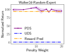
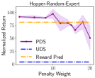
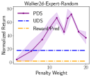
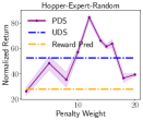
Figure 1: Impact of penalty weight $k$ on the performance. We evaluate PDS on Hopper/Walker2d-Labeled (Expert/Random)-Unlabeled (Expert/Random) tasks with various $k$.

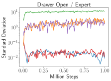
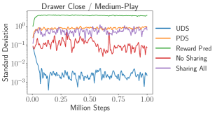
Figure 2: The standard deviation of the state values learned with IQL. The reward prediction method suffers from a large deviation. The oracle method’s and PDS’s deviation is mediocre, and no sharing and UDS methods enjoy the smallest deviation.

6 Conclusion

In this paper, we show that incorporating reward-free data into offline reinforcement learning can yield significant performance improvements. Our theoretical analysis reveals that unlabeled data provides additional information about the MDP’s dynamics, reducing the problem to linear bandits in the limit and improving performance bounds therefore. Building upon these insights, we propose a new algorithm, PDS, that leverages this information by incorporating uncertainty penalties on learned rewards to ensure a conservative approach. Our method has provable guarantees in theory and achieves superior performance in practice. In future work, it may be interesting to explore how PDS can be further improved with representation learning methods, and to extend our analysis to more general settings, such as generalized linear MDPs (Wang et al., 2019) and low-rank MDPs (Ayoub et al., 2020; Jiang et al., 2017).

7 Acknowledgements

This work is supported in part by Science and Technology Innovation 2030 - “New Generation Artificial Intelligence” Major Project (No. 2018AAA0100904) and the National Natural Science Foundation of China (62176135).

Appendix A Algorithm Details

A.1 Pessimistic Value Iteration (PEVI,(Jin et al., 2021))

In this section, we describe the details of PEVI algorithm.

In linear MDPs, we can construct $\widehat{\mathbb{B}}\widehat{V}$ and $\Gamma$ based on $\mathcal{D}$ as follows, where $\widehat{\mathbb{B}}\widehat{V}$ is the empirical estimation for $\mathbb{B}\widehat{V}$. For a given dataset $\mathcal{D}=\{(s_{\tau},a_{\tau},r_{\tau})\}_{\tau=1}^{N}$, we define the empirical mean squared Bellman error (MSBE) as

$$M(w)=\sum_{\tau=1}^{N}\bigl{(}r_{\tau}+\gamma\widehat{V}(s_{\tau+1})-\phi(s_{\tau},a_{\tau})^{\top}w\bigr{)}^{2}+\lambda||w||_{2}^{2}$$

Here $\lambda>0$ is the regularization parameter. Note that $\widehat{w}$ has the closed form

$$\widehat{w}=\Lambda^{-1}\Big{(}\sum_{\tau=1}^{N}\phi(s_{\tau},a_{\tau})\cdot\bigl{(}r_{\tau}+\gamma\widehat{V}(s_{\tau+1})\bigr{)}\Bigr{)},$$

$$\text{where~{}~{}}\Lambda=\lambda I+\sum_{\tau=1}^{N}\phi(s_{\tau},a_{\tau})\phi(s_{\tau},a_{\tau})^{\top}.$$ (18)

Then we simply let

$$\widehat{\mathbb{B}}\widehat{V}=\langle\phi,\widehat{w}\rangle.$$ (19)

Meanwhile, we construct $\Gamma$ based on $\mathcal{D}$ as

$$\Gamma(s,a)=\beta\cdot\big{(}\phi(s,a)^{\top}\Lambda^{-1}\phi(s,a)\big{)}^{1/2}.$$ (20)

Here $\beta>0$ is the scaling parameter. The overall PEVI algorithm is summarized in Algorithm 2.

Algorithm 2 Pessimistic Value Iteration, PEVI

1:  Require: Dataset $\mathcal{D}=\{(s_{\tau},a_{\tau},r_{\tau},s_{\tau+1})\}_{\tau=1}^{T}$.

2:  Initialization: Set $\widehat{V}(\cdot)\leftarrow 0$ and construct $\Gamma(\cdot,\cdot)$.

3:  while not converged do

4:     Construct $(\widehat{\mathbb{B}}\widehat{V})(\cdot,\cdot)$

5:     Set $\widehat{Q}(\cdot,\cdot)\leftarrow(\widehat{\mathbb{B}}\widehat{V})(\cdot,\cdot)-\Gamma(\cdot,\cdot)$.

6:     Set $\widehat{\pi}(\cdot{\,|\,}\cdot)\leftarrow\mathop{\mathrm{argmax}}_{\pi}\mathbb{E}_{\pi}{\left[\widehat{Q}(\cdot,\cdot)\right]}$.

7:     Set $\widehat{V}(\cdot)\leftarrow\mathbb{E}_{\widehat{\pi}}{\left[\widehat{Q}(\cdot,\cdot)\right]}$.

8:  end while

9:  Return $\widehat{V},\widehat{\pi}$

A.2 IQL with provable data sharing

In this section, we give a detailed description of our IQL+PDS algorithm.

Algorithm 3 IQL+PDS algorithm, General MDPs

Input: Labeled dataset $\mathcal{D}_{0}$, unlabeled dataset $\mathcal{D}_{1}$.
Input: Parameter $\alpha$, $\beta$, $k$, $\tau$.
Output: policy $\pi_{\phi}$.

1:  Learn $L$ reward functions as in Equation (7).

2:  Construct pessimistic reward estimation as in Equation (17).

3:  Relabel unsupervised dataset $\mathcal{D}_{1}$ and combine with the labeled dataset $\mathcal{D}_{0}$.

4:  Initialize $\psi$, $\theta$, $\widehat{\theta}$, $\phi$.

5:  for each gradient step do

6:     $\phi\leftarrow\psi-\lambda_{V}\nabla_{\psi}L_{V}(\psi),\quad L_{V}(\psi)=\mathbb{E}_{s,a}\left[L_{2}^{\tau}(Q_{\widehat{\theta}}(s,a)-V_{\psi}(s))\right]$

7:     $\theta\leftarrow\theta-\lambda_{Q}\nabla_{\theta}L_{Q}(\theta),\quad L_{Q}(\theta)=\mathbb{E}_{s,a,r}\left[(r+\gamma Q_{\widehat{\theta}}(s,a)-Q_{{\theta}}(s,a))^{2}\right]$

8:     $\widehat{\theta}\leftarrow\alpha\theta+(1-\alpha)\theta$

9:  end for

10:  for each gradient step do

11:     $\phi\leftarrow\phi-\lambda_{\pi}\nabla_{\phi}L_{\pi}(\phi),\quad L_{\pi}(\phi)=\mathbb{E}_{s,a}\left[\exp{\left(\beta(Q_{\widehat{\theta}}(s,a)-V_{\psi}(s))\right)}\log(\pi_{\phi}(a|s))\right]$

12:  end for

Appendix B Proof of Theorem 4.3

Proof.

From Equation (11) in Algorithm 1, we have

$$\widehat{V}_{\widetilde{\theta}}\leq\widehat{V}_{{\theta}},\quad\forall\theta\in\mathcal{C}(\delta),$$ (21)

where $\widetilde{\theta}$ is the pessimistic estimation of $\theta$.

Let $\mathcal{E}_{1}$ be the event $\theta^{\star}\in\mathcal{C}(\delta)$, then we have $\mathcal{P}(\mathcal{E}_{1})\geq 1-\delta$ from Lemma 4.1.

Let $\mathcal{E}_{2}$ be the event where the following inequality holds,

$$|(\mathbb{B}\widehat{V})(s,a)-(\widehat{\mathbb{B}}\widehat{V})(s,a)|\leq\Gamma=\beta\sqrt{\phi(s,a)^{\top}\Lambda^{-1}\phi(s,a)},\forall(s,a)\in{\mathcal{S}}\times\mathcal{A}.$$ (22)

then we have $\mathcal{P}(\mathcal{E}_{2})\geq 1-\delta$ from Lemma C.3.

Condition on $\mathcal{E}_{1}\cap\mathcal{E}_{2}$, we have.

$$V_{\theta^{\star}}^{\pi^{*}}-V_{\theta^{\star}}^{\widehat{\pi}} =V_{\theta^{\star}}^{\pi^{*}}-\widehat{V}_{\theta^{\star}}+\widehat{V}_{\theta^{\star}}-V_{\theta^{\star}}^{\widehat{\pi}}$$

$$\leq V_{\theta^{\star}}^{\pi^{*}}-\widehat{V}_{\theta^{\star}}$$

$$=V_{\theta^{\star}}^{\pi^{*}}-V_{\widetilde{\theta}}^{\pi^{*}}+V_{\widetilde{\theta}}^{\pi^{*}}-\widehat{V}_{\widetilde{\theta}}+\widehat{V}_{\widetilde{\theta}}-\widehat{V}_{\theta^{\star}}$$

$$\leq V_{\theta^{\star}}^{\pi^{*}}-V_{\widetilde{\theta}}^{\pi^{*}}+V_{\widetilde{\theta}}^{\pi^{*}}-\widehat{V}_{\widetilde{\theta}}$$

$$=V_{\theta^{\star}}^{\pi^{*}}-V_{\widehat{\theta}}^{\pi^{*}}+V_{\widehat{\theta}}^{\pi^{*}}-V_{\widetilde{\theta}}^{\pi^{*}}+V_{\widetilde{\theta}}^{\pi^{*}}-\widehat{V}_{\widetilde{\theta}}$$

$$\leq\frac{4r_{\text{\rm max}}}{1-\gamma}\sqrt{\frac{d^{2}\zeta_{2}}{N_{0}C_{0}^{\dagger}}}+\frac{2cr_{\text{\rm max}}}{(1-\gamma)^{2}}\sqrt{\frac{d^{3}\zeta_{1}}{N_{0}C_{0}^{\dagger}+N_{1}C_{1}^{\dagger}}},$$

where the first inequality follows from Lemma C.2. The second inequality follows from Equation (21), and the last inequality follows from Lemma C.5 and C.1.

From the union bound, we have that the above inequality holds with a probability of $1-2\delta$. ∎

Appendix C Addtional Lemmas and Missing Proofs

Lemma C.1.

Under the event in Lemma C.3, we have

$$V^{{\pi}^{*}}_{\theta}(s)-\widehat{V}_{\theta}(s) \leq\frac{2cr_{\text{max}}}{(1-\gamma)^{2}}\sqrt{\frac{d^{3}\zeta}{C^{\dagger}N}},$$

with probability $1-\delta$, for all $\|\theta\|_{2}^{2}\leq d$.

Proof.

Let

$$\delta(s,a)=r(s,a)+\gamma\mathbb{E}_{s^{\prime}\sim\mathcal{P}(\cdot|s,a)}\widehat{V}(s^{\prime})-\widehat{Q}(s,a),$$ (23)

From the definition of $\widehat{Q}(s,a)$ and $\widehat{V}(s)$, we have

$$\delta(s,a)=\mathbb{B}_{\gamma}\widehat{V}(s)-\widehat{Q}(s,a)=\mathbb{B}_{\gamma}\widehat{V}(s)-\widehat{\mathbb{B}}_{\gamma}\widehat{V}+\Gamma(s,a).$$ (24)

Under the condition of Lemma C.3, it holds that

$$0\leq\delta(s,a)\leq 2\Gamma(s,a),\text{for all}~{}s,a.$$ (25)

Then we have

$$V^{{\pi}^{*}}_{\theta}(s)-\widehat{V}_{\theta}(s)$$

$$= \mathbb{E}_{a\sim{\pi}^{*},s^{\prime}\sim\mathcal{P}(\cdot|s,a)}\left[r(s,a)+\gamma V^{{\pi}^{*}}(s^{\prime})\right]-\mathbb{E}_{a\sim\widehat{\pi}}\left[\widehat{Q}(s,a)\right]$$

$$= \mathbb{E}_{a\sim{\pi}^{*},s^{\prime}\sim\mathcal{P}(\cdot|s,a)}\left[r(s,a)+\gamma V^{{\pi}^{*}}(s^{\prime})-\widehat{Q}(s,a)\right]+\mathbb{E}_{a\sim{\pi}^{*}}\left[\widehat{Q}(s,a)\right]-\mathbb{E}_{a\sim\widehat{\pi}}\left[\widehat{Q}(s,a)\right]$$

$$= \mathbb{E}_{a\sim{\pi}^{*},s^{\prime}\sim\mathcal{P}(\cdot|s,a)}\left[r(s,a)+\gamma\widehat{V}(s^{\prime})-\widehat{Q}(s,a)\right]+\gamma\mathbb{E}_{a\sim{\pi}^{*},s^{\prime}\sim\mathcal{P}(\cdot|s,a)}\left[V^{{\pi}^{*}}(s^{\prime})-\widehat{V}(s^{\prime})\right]$$

$$+\left\langle\widehat{Q}(s,\cdot),\pi^{*}(\cdot{\,|\,}s)-\widehat{\pi}(\cdot{\,|\,}s)\right\rangle_{\mathcal{A}}$$

$$= \mathbb{E}_{a\sim{\pi}^{*},s^{\prime}\sim\mathcal{P}(\cdot|s,a)}\left[\delta(s,a)\right]+\left\langle\widehat{Q}(s,\cdot),\pi^{*}(\cdot{\,|\,}s)-\widehat{\pi}(\cdot{\,|\,}s)\right\rangle_{\mathcal{A}}+\cdots$$

$$= \mathbb{E}_{\pi^{*}}\left[\sum_{t=0}^{\infty}\gamma^{t}\delta(s_{t},a_{t}){\,|\,}s_{0}=s\right]+\mathbb{E}_{\pi^{*}}\left[\sum_{t=0}^{\infty}\gamma^{t}\left\langle\widehat{Q}(s_{t},\cdot),\pi^{*}(\cdot{\,|\,}s_{t})-\widehat{\pi}(\cdot{\,|\,}s_{t})\right\rangle_{\mathcal{A}}{\,|\,}s_{0}=s\right]$$

$$\leq \mathbb{E}_{\pi^{*}}\left[\sum_{t=0}^{\infty}{\gamma^{t}\delta(s_{t},a_{t})}\,\Big{|}\,s_{0}=s\right]$$

$$\leq 2\mathbb{E}_{\pi^{*}}\Bigl{[}\sum_{t=0}^{\infty}\gamma^{t}\Gamma(s_{t},a_{t})\,\Big{|}\,s_{0}=s\Bigr{]}$$

$$= 2\beta\mathbb{E}_{\pi^{*}}\Bigl{[}\sum_{t=0}^{\infty}\gamma^{t}\bigl{(}\phi(s_{t},a_{t})^{\top}\Lambda^{-1}\phi(s_{t},a_{t})\bigr{)}^{1/2}\,\Big{|}\,s_{0}=s\Bigr{]}.$$

Here the first inequality follows from the fact that $\widehat{\pi}(\cdot|s)=\mathop{\mathrm{argmax}}_{\pi}\left\langle\widehat{Q}(\cdot,\cdot),\pi(\cdot|s)\right\rangle$ and the second inequality follows from Equation (25).

By the Cauchy-Schwarz inequality, we have

$$\mathbb{E}_{\pi^{*}}\Bigl{[}\sum_{t=0}^{\infty}\gamma^{t}\bigl{(}\phi(s_{t},a_{t})^{\top}\Lambda^{-1}\phi(s_{t},a_{t})\bigr{)}^{1/2}\,\Big{|}\,s_{0}=s\Bigr{]}$$

$$\qquad=\frac{1}{1-\gamma}\mathbb{E}_{d^{\pi^{*}}}\Bigl{[}\sqrt{\mathop{\text{Tr}}\kern 0.86108pt\big{(}\phi(s,a)^{\top}\Lambda^{-1}\phi(s,a)\big{)}}\,\Big{|}\,s_{0}=s\Bigr{]}$$

$$\qquad=\frac{1}{1-\gamma}\mathbb{E}_{d^{\pi^{*}}}\Bigl{[}\sqrt{\mathop{\text{Tr}}\kern 0.86108pt\big{(}\phi(s,a)\phi(s,a)^{\top}\Lambda^{-1}\big{)}}\,\Big{|}\,s_{0}=s\Bigr{]}$$

$$\qquad\leq\frac{1}{1-\gamma}\sqrt{\mathop{\text{Tr}}\kern 0.86108pt\Big{(}\mathbb{E}_{d^{\pi^{*}}}\big{[}\phi(s,a)\phi(s,a)^{\top}\,\big{|}\,s_{0}=s\big{]}\Lambda^{-1}\Big{)}}$$

$$\qquad=\frac{1}{1-\gamma}\sqrt{\mathop{\text{Tr}}\kern 0.86108pt\Big{(}\Sigma_{\pi^{*},s}^{\top}\Lambda^{-1}\Big{)}},$$ (26)

for all $s\in{\mathcal{S}}$. Then we have

$$V^{{\pi}^{*}}_{\theta}(s)-\widehat{V}_{\theta}(s) \leq 2\beta\mathbb{E}_{\pi^{*}}\Bigl{[}\sum_{t=0}^{\infty}\gamma^{t}\bigl{(}\phi(s_{t},a_{t})^{\top}\Lambda^{-1}\phi(s_{t},a_{t})\bigr{)}^{1/2}\,\Big{|}\,s_{0}=s\Bigr{]}$$

$$\leq\frac{2\beta}{1-\gamma}\sqrt{\mathop{\text{Tr}}\kern 0.86108pt\Big{(}\Sigma_{\pi^{*},s}\cdot\big{(}I+{C^{\dagger}}\cdot N\cdot\Sigma_{\pi^{*},s}\big{)}^{-1}\Big{)}}$$

$$=\frac{2\beta}{1-\gamma}\sqrt{\sum_{j=1}^{d}\frac{\lambda_{j}(s)}{1+{C^{\dagger}}\cdot N\cdot\lambda_{j}(s)}}.$$ (27)

Here $\{\lambda_{j}(s)\}_{j=1}^{d}$ are the eigenvalues of $\Sigma_{\pi^{*},s}$ for all $s\in{\mathcal{S}}$, the second inequality follows from Equation (C). Meanwhile, by Definition 3.1, we have $\|\phi(s,a)\|\leq 1$ for all $(s,a)\in{\mathcal{S}}\times\mathcal{A}$. By Jensen’s inequality, we have

$$\|\Sigma_{\pi^{*},s}\|_{\mathop{\text{op}}}\leq\mathbb{E}_{\pi^{*}}\big{[}\|\phi(s,a)\phi(s,a)^{\top}\|_{\mathop{\text{op}}}\,\big{|}\,s_{0}=s\big{]}\leq 1$$ (28)

for all $s\in{\mathcal{S}}$. As $\Sigma_{\pi^{*},s}$ is positive semidefinite, we have $\lambda_{j}(s)\in[0,1]$ for all $s\in{\mathcal{S}}$ and all $j\in[d]$. Hence we have

$$V^{{\pi}^{*}}_{\theta}(s)-\widehat{V}_{\theta}(s) \leq\frac{2\beta}{1-\gamma}\sqrt{\sum_{j=1}^{d}\frac{\lambda_{j}(s)}{1+{C^{\dagger}}\cdot N\cdot\lambda_{j}(s)}}$$

$$\leq\frac{2\beta}{1-\gamma}\sqrt{\sum_{j=1}^{d}\frac{1}{1+{C^{\dagger}}\cdot N}}\leq\frac{2cr_{\text{max}}}{(1-\gamma)^{2}}\sqrt{\frac{d^{3}\zeta}{C^{\dagger}N}}$$ (29)

for all $x\in{\mathcal{S}}$, where the second inequality follows from the fact that $\lambda_{j}(s)\in[0,1]$ for all $s\in{\mathcal{S}}$ and all $j\in[d]$, while the third inequality follows from the choice of the scaling parameter $\beta>0$.

Then we have the conclusion in Lemma C.1. ∎

Lemma C.2.

Under the event in Lemma C.3, we have

$$\widehat{V}_{\theta}(s)-V^{\widehat{\pi}_{\theta}}(s)\leq 0$$ (30)

with probability $1-\delta$, for all $\|\theta\|_{2}^{2}\leq d$.

Proof.

Similar to the proof of Lemma C.1, let

$$\delta(s,a)=r(s,a)+\gamma\mathbb{E}_{s^{\prime}\sim\mathcal{P}(\cdot|s,a)}\widehat{V}(s^{\prime})-\widehat{Q}(s,a),$$ (31)

we have

$$\widehat{V}(s)-V^{\widehat{\pi}}(s)= \mathbb{E}_{a\sim\widehat{\pi}}\left[\widehat{Q}(s,a)\right]-\mathbb{E}_{a\sim\widehat{\pi},s^{\prime}\sim\mathcal{P}(\cdot|s,a)}\left[r(s,a)+\gamma V^{\widehat{\pi}}(s^{\prime})\right]$$

$$= \mathbb{E}_{a\sim\widehat{\pi},s^{\prime}\sim\mathcal{P}(\cdot|s,a)}\left[\widehat{Q}(s,a)-r(s,a)-\gamma\widehat{V}(s^{\prime})\right]$$

$$+\gamma\mathbb{E}_{a\sim\widehat{\pi},s^{\prime}\sim\mathcal{P}(\cdot|s,a)}\left[\widehat{V}(s^{\prime})-V^{\widehat{\pi}}(s^{\prime})\right]$$

$$= -\mathbb{E}_{\widehat{\pi}}\left[\delta(s,a)\right]+\gamma\mathbb{E}_{a\sim\widehat{\pi},s^{\prime}\sim\mathcal{P}(\cdot|s,a)}\left[\widehat{V}(s^{\prime})-V^{\widehat{\pi}}(s^{\prime})\right]$$

$$= -\mathbb{E}_{\widehat{\pi}}\left[\delta(s,a)\right]+\cdots$$

$$= -\mathbb{E}_{\widehat{\pi}}\left[\sum_{t=0}^{\infty}\gamma^{t}\delta(s_{t},a_{t}){\,|\,}s_{0}=s\right].$$

Then under the condition of Lemma C.3, it holds that

$$0\leq\delta(s,a)\leq 2\Gamma(s,a),\text{for all}~{}s,a,$$ (32)

Then we have the result immediately.

∎

Lemma C.3 ($\xi$-Quantifiers).

Let

$$\lambda=1,\quad\beta=c\cdot dV_{\text{max}}\sqrt{\zeta},\quad\zeta=\log{(2dN/(1-\gamma)\xi)}.$$ (33)

Then $\Gamma=\beta\cdot\big{(}\phi(s,a)^{\top}\Lambda^{-1}\phi(s,a)\big{)}^{1/2}$ are $\xi$-quantifiers with probability at least $1-\xi$. That is, let $\mathcal{E}_{2}$ be the event that the following inequality holds,

$$|(\mathbb{B}\widehat{V})(s,a)-(\widehat{\mathbb{B}}\widehat{V})(s,a)|\leq\Gamma=\beta\sqrt{\phi(s,a)^{\top}\Lambda^{-1}\phi(s,a)},\forall(s,a)\in{\mathcal{S}}\times\mathcal{A}.$$ (34)

Then we have $\mathcal{P}(\mathcal{E}_{2})\geq 1-\varepsilon$.

Proof.

we have

$$\mathbb{B}\widehat{V}-\widehat{\mathbb{B}}\widehat{V} =\phi(s,a)^{\top}(w-\widehat{w})$$

$$=\phi(s,a)^{\top}w-\phi(s,a)\Lambda^{-1}\left(\sum_{\tau=1}^{N}{\phi_{\tau}(r_{\tau}+\gamma\widehat{V}(s_{\tau+1})}\right)$$

$$=\underbrace{\phi(s,a)^{\top}w-\phi(s,a)\Lambda^{-1}\left(\sum_{\tau=1}^{N}{\phi_{\tau}\phi_{\tau}^{\top}w}\right)}_{\displaystyle\text{(i)}}+\underbrace{\phi(s,a)\Lambda^{-1}(\sum_{\tau=1}^{N}{\phi_{\tau}\phi_{\tau}^{\top}w}-\sum_{\tau=1}^{N}\phi_{\tau}(r_{\tau}+\gamma\widehat{V}(s_{\tau+1}))}_{\displaystyle\text{(ii)}},$$ (35)

Then we bound (i) and (ii), respectively.

For (i), we have

(i) $$=\phi(s,a)^{\top}w-\phi(s,a)\Lambda^{-1}(\Lambda-\lambda I)w$$

$$=\lambda\phi(s,a)\Lambda^{-1}w$$

$$\leq\lambda||\phi(s,a)||_{\lambda^{-1}}||w||_{\lambda^{-1}}$$

$$\leq V_{\text{max}}\sqrt{d\lambda}\sqrt{\phi(s,a)^{\top}\Lambda^{-1}\phi(s,a)},$$ (36)

where the first inequality follows from Cauchy-Schwartz inequality. The second inequality follows from the fact that $||\Lambda^{-1}||_{\text{op}}\leq\lambda^{-1}$ and Lemma C.4.

For notation simplicity, let $\epsilon_{\tau}=r_{\tau}+\gamma\widehat{V}(s_{\tau+1})-\phi_{\tau}^{\top}w$, then we have

$$|\text{(ii)}| =\phi(s,a)\Lambda^{-1}\sum_{\tau=1}^{N}{\phi_{\tau}\epsilon_{\tau}}$$

$$\leq||\sum_{\tau=1}^{N}{\phi_{\tau}\epsilon_{\tau}}||_{\Lambda^{-1}}\cdot||\phi(s,a)||_{\Lambda^{-1}}$$

$$=\underbrace{||\sum_{\tau=1}^{N}{\phi_{\tau}\epsilon_{\tau}}||_{\Lambda^{-1}}}_{\text{(iii)}}\cdot\sqrt{\phi(s,a)^{\top}\Lambda^{-1}\phi(s,a)}.$$ (37)

The term (iii) is depend on the randomness of the data collection process of $\mathcal{D}$. To bound this term, we resort to uniform concentration inequalities to upper bound

$$\sup_{V\in\mathcal{V}(R,B,\lambda)}\Big{\|}\sum_{\tau=1}^{N}\phi(s_{\tau},a_{\tau})\cdot\epsilon_{\tau}(V)\Big{\|},$$

where

$$\mathcal{V}(R,B,\lambda)=\{V(s;w,\beta,\Sigma):\mathcal{S}\rightarrow[0,V_{\text{max}}]~{}\text{with}||w||\leq R,\beta\in[0,B],\Sigma\succeq\lambda\cdot I\},$$ (38)

where $V(s;w,\beta,\Sigma)=\max_{a}\{\phi(s,a)^{\top}w-\beta\cdot\sqrt{\phi(s,a)^{\top}\Sigma^{-1}\phi(s,a)}\}$. For all $\epsilon>0$, let $\mathcal{N}(\epsilon;R,B,\lambda)$ be the minimal cover if $\mathcal{V}(R,B,\lambda)$. That is, for any function $V\in\mathcal{V}(R,B,\lambda)$, there exists a function $V^{\dagger}\in\mathcal{N}(\epsilon;R,B,\lambda)$, such that

$$\sup_{s\in{\mathcal{S}}}{|V(s)-V^{\dagger}(s)|\leq\epsilon}.$$ (39)

Let $R_{0}=V_{\text{max}}\sqrt{Nd/\lambda},B_{0}=2\beta$, it is easy to show that at each iteration, $\widehat{V}^{u}\in\mathcal{V}(R_{0},B_{0},\lambda)$. From the definition of $\mathbb{B}$, we have

$$|\mathbb{B}\widehat{V}-\mathbb{B}V^{\dagger}|=\gamma\left|\int{(\widehat{V}(s^{\prime})-V^{\dagger}(s^{\prime}))\left\langle\phi(s,a),\mu(s^{\prime})\right\rangle{\mathrm{d}}s^{\prime}}\right|\leq\gamma\epsilon.$$ (40)

Then we have

$$|(r+\gamma V-\mathbb{B}V)-(r+\gamma V^{\dagger}-\mathbb{B}V^{\dagger})|\leq 2\gamma\epsilon.$$ (41)

Let $\epsilon_{\tau}^{\dagger}=r(s_{\tau},a_{\tau})+\gamma V^{\dagger}(s_{\tau+1})-\mathbb{B}V^{\dagger}(s,a)$, we have

$$\text{(iii)}^{2}=||\sum_{\tau=1}^{N}\phi_{\tau}\epsilon_{\tau}||^{2}_{\Lambda^{-1}} \leq 2||\sum_{\tau=1}^{N}\phi_{\tau}\epsilon^{\dagger}_{\tau}||^{2}_{\Lambda^{-1}}+2||\sum_{\tau=1}^{N}\phi_{\tau}(\epsilon^{\dagger}_{\tau}-\epsilon_{\tau})||^{2}_{\Lambda^{-1}}$$

$$\leq 2||\sum_{\tau=1}^{N}\phi_{\tau}\epsilon^{\dagger}_{\tau}||^{2}_{\Lambda^{-1}}+8\gamma^{2}\epsilon^{2}\sum_{\tau=1}^{N}|\phi_{\tau}\Lambda^{-1}\phi_{\tau}|$$

$$\leq 2||\sum_{\tau=1}^{N}\phi_{\tau}\epsilon^{\dagger}_{\tau}||^{2}_{\Lambda^{-1}}+8\gamma^{2}\epsilon^{2}N^{2}/\lambda$$

It remains to bound $||\sum_{\tau=1}^{N}\phi_{\tau}\epsilon^{\dagger}_{\tau}||^{2}_{\Lambda^{-1}}$. From the assumption for data collection process, it is easy to show that $\mathbb{E}_{\mathcal{D}}{[\epsilon_{\tau}{\,|\,}\mathcal{F}_{\tau-1}]}=0$, where $F_{\tau-1}=\sigma(\{(s_{i},a_{i})_{i=1}^{\tau}\cup(r_{i},s_{i+1})_{i=1}^{\tau}\})$ is the $\sigma$-algebra generated by the variables from the first $\tau$ step. Moreover, since $\epsilon_{\tau}\leq 2V_{\text{max}}$, we have $\epsilon_{\tau}$ are $2V_{\text{max}}$-sub-Gaussian conditioning on $F_{\tau-1}$. Then we invoke Lemma C.7 with $M_{0}=\lambda\cdot I$ and $M_{k}=\lambda\cdot I+\sum_{\tau=1}^{k}\phi(s_{\tau},a_{\tau})\ \phi(s_{\tau},a_{\tau})^{\top}$. For the fixed function $V\colon{\mathcal{S}}\to[0,V_{\text{max}}]$, we have

$$\mathbb{P}_{\mathcal{D}}\bigg{(}\Big{\|}\sum_{\tau=1}^{N}\phi(s_{\tau},a_{\tau})\cdot\epsilon_{\tau}(V)\Big{\|}_{\Lambda^{-1}}^{2}>8V^{2}_{\text{max}}\cdot\log\Big{(}\frac{\det(\Lambda)^{1/2}}{\delta\cdot\det(\lambda\cdot I)^{1/2}}\Big{)}\bigg{)}\leq\delta$$ (42)

for all $\delta\in(0,1)$. Note that $\|\phi(s,a)\|\leq 1$ for all $(s,a)\in{\mathcal{S}}\times\mathcal{A}$ by Definition 3.1. We have

$$\|\Lambda\|_{\mathop{\text{op}}}=\Big{\|}\lambda\cdot I+\sum_{\tau=1}^{N}\phi(s_{\tau},a_{\tau})\phi(s_{\tau},a_{\tau})^{\top}\Big{\|}_{\mathop{\text{op}}}\leq\lambda+\sum_{\tau=1}^{N}\|\phi(s_{\tau},a_{\tau})\phi(s_{\tau},a_{\tau})^{\top}\|_{\mathop{\text{op}}}\leq\lambda+N,$$

where $\|\cdot\|_{\mathop{\text{op}}}$ denotes the matrix operator norm. Hence, it holds that $\det(\Lambda)\leq(\lambda+N)^{d}$ and $\det(\lambda\cdot I)=\lambda^{d}$, which implies

$$\mathbb{P}_{\mathcal{D}}\bigg{(}\Big{\|}\sum_{\tau=1}^{N}\phi(s_{\tau},a_{\tau})\cdot\epsilon_{\tau}(V)\Big{\|}_{\Lambda_{-1}}^{2}>4V^{2}_{\text{max}}\cdot\bigl{(}2\cdot\log(1/\delta)+d\cdot\log(1+N/\lambda)\big{)}\biggr{)}$$

$$\qquad\leq\mathbb{P}_{\mathcal{D}}\bigg{(}\Big{\|}\sum_{\tau=1}^{N}\phi(s_{\tau},a_{\tau})\cdot\epsilon_{\tau}(V)\Big{\|}_{\Lambda_{-1}}^{2}>8V^{2}_{\text{max}}\cdot\log\Big{(}\frac{\det(\Lambda)^{1/2}}{\delta\cdot\det(\lambda\cdot I)^{1/2}}\Big{)}\bigg{)}\leq\delta.$$

Therefore, we conclude the proof of Lemma C.3.

Applying Lemma C.3 and the union bound, we have

$$\mathbb{P}_{\mathcal{D}}\bigg{(}\sup_{V\in\mathcal{N}(\varepsilon)}\Big{\|}\sum_{\tau=1}^{N}\phi(s_{\tau},a_{\tau})\cdot\epsilon_{\tau}(V)\Big{\|}_{\Lambda^{-1}}^{2}>4V^{2}_{\text{max}}\cdot\bigl{(}2\cdot\log(1/\delta)+d\cdot\log(1+N/\lambda)\big{)}\biggr{)}\leq\delta\cdot|\mathcal{N}(\varepsilon)|.$$ (43)

Recall that

$$\widehat{V}\in\mathcal{V}(R_{0},B_{0},\lambda),\qquad\text{where}~{}~{}R_{0}=V_{\text{max}}\sqrt{Nd/\lambda},~{}B_{0}=2\beta,~{}\lambda=1,~{}\beta=c\cdot dV_{\text{max}}\sqrt{\zeta}.$$ (44)

Here $c>0$ is an absolute constant, $\xi\in(0,1)$ is the confidence parameter, and $\zeta=\log(2dV_{\text{max}}/\xi)$ is specified in Algorithm 2. Applying Lemma C.6 with $\varepsilon=dV_{\text{max}}/N$, we have

$$\log|\mathcal{N}(\varepsilon)| \leq d\cdot\log(1+4d^{-1/2}N^{3/2})+d^{2}\cdot\log(1+32c^{2}\cdot d^{1/2}N^{2}\zeta)$$

$$\leq d\cdot\log(1+4d^{1/2}N^{2})+d^{2}\cdot\log(1+32c^{2}\cdot d^{1/2}N^{2}\zeta).$$ (45)

By setting $\delta=\xi/|\mathcal{N}(\varepsilon)|$, we have that with probability at least $1-\xi$,

$$\Big{\|}\sum_{\tau=1}^{N}\phi(s_{\tau},a_{\tau})\cdot\epsilon_{\tau}(\widehat{V})\Big{\|}_{\Lambda^{-1}}^{2}$$

$$\qquad\leq 8V_{\text{max}}^{2}\cdot\bigl{(}2\cdot\log(V_{\text{max}}/\xi)+4d^{2}\cdot\log(64c^{2}\cdot d^{1/2}N^{2}\zeta)+d\cdot\log(1+N)+4d^{2}\bigr{)}$$

$$\qquad\leq 8V_{\text{max}}^{2}d^{2}\zeta(4+\log{(64c^{2})}).$$ (46)

Here the last inequality follows from simple algebraic inequalities. We set $c\geq 1$ to be sufficiently large, which ensures that $36+8\cdot\log(64c^{2})\leq c^{2}/4$ on the right-hand side of Equation (C). By Equations (C) and (C), it holds that

$$|\text{(ii)}|\leq c/2\cdot dV_{\text{max}}\sqrt{\zeta}\cdot\sqrt{\phi(x,a)^{\top}\Lambda^{-1}\phi(s,a)}=\beta/2\cdot\sqrt{\phi(x,a)^{\top}\Lambda^{-1}\phi(s,a)}$$ (47)

By Equations (20), (35), (C), and (47), for all $(s,a)\in{\mathcal{S}}\times\mathcal{A}$, it holds that

$$\bigl{|}(\mathbb{B}\widehat{V})(s,a)-(\widehat{\mathbb{B}}\widehat{V})(s,a)\bigr{|}\leq(V_{\text{max}}\sqrt{d}+\beta/2)\cdot\sqrt{\phi(s,a)^{\top}\Lambda^{-1}\phi(s,a)}\leq\Gamma(s,a)$$ (48)

with probability at least $1-\xi$. Therefore, we conclude the proof of Lemma C.3. ∎

Lemma C.4 (Bounded weight of value function).

Let $V_{\text{\rm max}}=r_{\text{\rm max}}/(1-\gamma)$. For any function $V:{\mathcal{S}}\rightarrow[0,V_{\text{\rm max}}]$, we have

$$||w||\leq V_{\text{\rm max}}\sqrt{d},||\widehat{w}||\leq V_{\text{\rm max}}\sqrt{\frac{Nd}{\lambda}}.$$

Proof.

Since

$$w^{\top}\phi(s,a)=\left\langle M,\phi(s,a)\right\rangle+\gamma\int{V(s^{\prime})\psi(s^{\prime})^{\top}M\phi(s,a){\mathrm{d}}s^{\prime}},$$

we have

$$w =M+\gamma\int{V(s^{\prime})\psi(s^{\prime})^{\top}M{\mathrm{d}}s^{\prime}}$$

$$=r_{\text{max}}\sqrt{d}+\gamma V_{\text{max}}\sqrt{d}$$

$$=V_{\text{max}}\sqrt{d}.$$

For $\widehat{w}$, we have

$$||\widehat{w}|| =||\Lambda^{-1}\sum_{\tau=1}^{N}{\phi_{\tau}(r_{\tau}+\gamma V(s_{\tau+1}))}||$$

$$\leq\sum_{\tau=1}^{N}{||\Lambda^{-1}{\phi_{\tau}(r_{\tau}+\gamma V(s_{\tau+1}))}||}$$

$$\leq V_{\text{max}}\sum_{\tau=1}^{N}{||\Lambda^{-1}{\phi_{\tau}}||}$$

$$\leq V_{\text{max}}\sum_{\tau=1}^{N}{\sqrt{\phi_{\tau}^{\top}\Lambda^{-1/2}\Lambda^{-1}\Lambda^{-1/2}\phi_{\tau}}}$$

$$\leq\frac{V_{\text{max}}}{\sqrt{\lambda}}\sum_{\tau=1}^{N}{\sqrt{\phi_{\tau}^{\top}\Lambda^{-1}\phi_{\tau}}}$$

$$\leq V_{\text{max}}\sqrt{\frac{N}{\lambda}}\sqrt{\mathrm{Tr}(\Lambda^{-1}\sum_{\tau=1}^{T}{\phi_{\tau}\phi_{\tau}^{\top}})}$$

$$\leq V_{\text{max}}\sqrt{\frac{Nd}{\lambda}}.$$

∎

Lemma C.5.

For policy $\pi^{*}$ and any reward function parameter $\theta\in\mathcal{C}(\delta)$, we have

$$|V^{\pi^{*}}_{\theta}-V^{\pi^{*}}_{\widehat{\theta}}|\leq\frac{2r_{\text{max}}}{1-\gamma}\sqrt{\frac{d^{2}\zeta_{2}}{N_{0}C^{\dagger}_{0}}}.$$

Proof.

From the definition, we have

$$|r_{\theta}(s,a)-r_{\widehat{\theta}}(s,a)| =|\phi(s,a)^{\top}\theta-\phi(s,a)^{\top}\widehat{\theta}|$$

$$\leq\|\theta-\widehat{\theta}\|_{\Lambda}\cdot\|\phi(s,a)\|_{\Lambda^{-1}}$$

$$\leq\alpha\sqrt{\phi(s,a)^{\top}\Lambda^{-1}\phi(s,a)},$$

Where the first inequality follows from the Cauchy-Schwartz inequality and the second inequality uses the fact that $\theta\in\mathcal{C}(\delta)$. Then we have

$$V^{\pi^{*}}_{\theta}(s)-V^{\pi^{*}}_{\widehat{\theta}}(s) =\mathbb{E}_{{\pi^{*}}}\left[\sum_{t=0}^{\infty}\gamma^{t}(r_{\theta}(s,a)-r_{\widehat{\theta}}(s,a))\,\Big{|}\,s_{0}=s\right]$$

$$\leq\mathbb{E}_{{\pi^{*}}}\left[\sum_{t=0}^{\infty}\gamma^{t}|r_{\theta}(s,a)-r_{\widehat{\theta}}(s,a)|\,\Big{|}\,s_{0}=s\right]$$

$$\leq\alpha\mathbb{E}_{{\pi^{*}}}\left[\sum_{t=0}^{\infty}\gamma^{t}\sqrt{\phi(s,a)^{\top}\Lambda^{-1}\phi(s,a)}\,\Big{|}\,s_{0}=s\right]$$

$$\leq\frac{\alpha}{1-\gamma}\sqrt{\sum_{j=1}^{d}\frac{1}{1+C_{0}^{\dagger}\cdot N_{0}}}\leq\frac{2r_{\text{max}}}{1-\gamma}\sqrt{\frac{d^{2}\zeta_{2}}{N_{0}C_{0}^{\dagger}}},$$

where the second to last inequality follows similarly as Equation (C) (C) and the last inequality follows from the fact that $\alpha=2r_{\text{\rm max}}\sqrt{d\zeta_{2}}$.

Note that such a choice of $\alpha$ is sufficient for Lemma 4.1 to hold since

$$\sqrt{\nu}+r_{\text{\rm max}}\cdot\sqrt{2\log{\frac{1}{\delta}}+d\log{(1+\frac{N_{0}}{\nu d})}} =1+r_{\text{\rm max}}\cdot\sqrt{2\log{\frac{1}{\delta}}+d\log{(1+\frac{N_{0}}{d})}}$$

$$\leq 1+r_{\text{\rm max}}\cdot\sqrt{2\log{\frac{1}{\delta}}+d\log{2N_{0}}}$$

$$\leq 1+r_{\text{\rm max}}\cdot\sqrt{d\log{\frac{2N_{0}}{\delta}}}$$

$$\leq 2r_{\text{\rm max}}\cdot\sqrt{d\log{\frac{2N_{0}}{\delta}}}$$

$$=2r_{\text{\rm max}}\sqrt{d\zeta_{2}},$$

where the inequalities holds for sufficiently small $\delta>0$ and $d\geq 2$. ∎

C.1 Technical Lemmas

Lemma C.6 ($\varepsilon$-Covering Number (Jin et al., 2020)).

For all $h\in[H]$ and all $\varepsilon>0$, we have

$$\log|\mathcal{N}(\varepsilon;R,B,\lambda)|\leq d\cdot\log(1+4R/\varepsilon)+d^{2}\cdot\log\bigl{(}1+8d^{1/2}B^{2}/(\varepsilon^{2}\lambda)\bigr{)}.$$

Proof of Lemma C.6.

See Lemma D.6 in Jin et al. (2020) for detailed proof. ∎

Lemma C.7 (Concentration of Self-Normalized Processes (Abbasi-Yadkori et al., 2011)).

Let $\{\mathcal{F}_{t}\}^{\infty}_{t=0}$ be a filtration and $\{\epsilon_{t}\}^{\infty}_{t=1}$ be an $\mathbb{R}$-valued stochastic process such that $\epsilon_{t}$ is $\mathcal{F}_{t}$-measurable for all $t\geq 1$. Moreover, suppose that conditioning on $\mathcal{F}_{t-1}$, $\epsilon_{t}$ is a zero-mean and $\sigma$-sub-Gaussian random variable for all $t\geq 1$, that is,

$$\mathbb{E}[\epsilon_{t}{\,|\,}\mathcal{F}_{t-1}]=0,\qquad\mathbb{E}\bigl{[}\exp(\lambda\epsilon_{t})\,\big{|}\,\mathcal{F}_{t-1}\bigr{]}\leq\exp(\lambda^{2}\sigma^{2}/2),\qquad\forall\lambda\in\mathbb{R}.$$

Meanwhile, let $\{\phi_{t}\}_{t=1}^{\infty}$ be an $\mathbb{R}^{d}$-valued stochastic process such that $\phi_{t}$ is $\mathcal{F}_{t-1}$-measurable for all $t\geq 1$. Also, let $M_{0}\in\mathbb{R}^{d\times d}$ be a deterministic positive-definite matrix and

$$M_{t}=M_{0}+\sum_{s=1}^{t}\phi_{s}\phi_{s}^{\top}$$

for all $t\geq 1$. For all $\delta>0$, it holds that

$$\Big{\|}\sum_{s=1}^{t}\phi_{s}\epsilon_{s}\Big{\|}_{M_{t}^{-1}}^{2}\leq 2\sigma^{2}\cdot\log\Bigl{(}\frac{\det(M_{t})^{1/2}\cdot\det(M_{0})^{-1/2}}{\delta}\Bigr{)}$$

for all $t\geq 1$ with probability at least $1-\delta$.

Proof.

See Theorem 1 of Abbasi-Yadkori et al. (2011) for a detailed proof. ∎

Appendix D Experimental Settings

D.1 Multi-task Antmaze

We first divide the source dataset (e.g., antmaze-medium-diverse-v2) into the directed dataset or the undirected dataset. The trajectories in the undirected dataset are randomly and uniformly divided into different tasks. In contrast, the directed dataset is associated with the goal closest to the final state of the trajectory. Then, for each subtask (e.g., goal=(0.0, 16.0)), we relabel the corresponding undirected or undirected dataset according to the goal. Finally, we keep the rewards in the target task dataset (labeled dataset) while setting the rewards in the other task dataset to 0 (unlabeled dataset). We visualize the directed or undirected dataset in Figure 3. We can find that the distribution shift issue in the directed dataset is more severe than the undirected dataset, which further challenges the unlabeled data sharing algorithms.

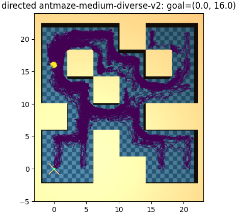
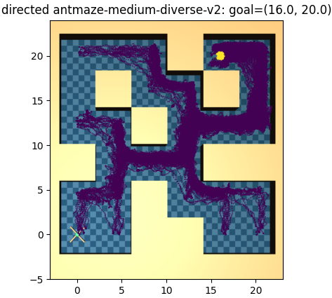
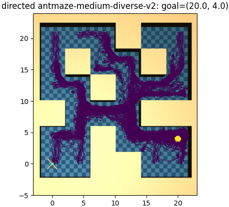
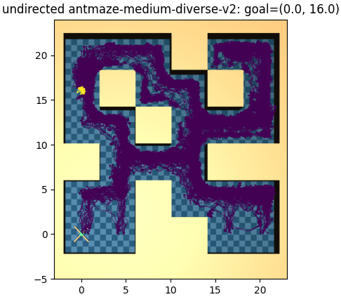
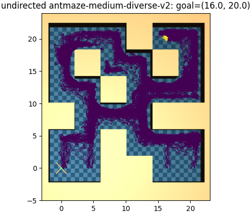
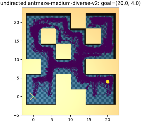
Figure 3: Visualization of multi-task antmaze-medium-diverse-v2 datasets. The purple dots denote the transition of reward 0. The yellow dots denote the transition near the goal of the sub-task and the reward is +1.

D.2 Multi-task Meta-World

We consider the same setup as in CDS (Yu et al., 2021a) and four tasks: door open, door close, drawer open and drawer close, which is shown in Figure 4. We use medium-replay datasets with 152K transitions for task door open and drawer close and use 10 expert trajectories for task door close and drawer open.

(a) Door Open

(b) Drawer Close

Figure 4: Visualization of subtasks in Meta-World.

Appendix E More discussion on the relative performance of UDS

Based on the discussion in the main text, we can summarize the factors that affect the relative performance of PDS algorithms as follows.

scenarios	large number of unlabeled data	high quality of unlabeled data	long horizon	large dimension
finite-sample term	✓	✓
asymptotic term			✓	✓

Table 4: Scenarios where PDS has better relative performance.

However, it is worth noting that the asymptotic term is dependent on the backbone offline algorithm we choose. For model-based algorithms like Uehara & Sun (2021), the performance bound scale as $\mathcal{O}(d)$ and thus the problem’s dimension does not affect the asymptotic term. The dependence over the discount factor is also dependent on the choice of the backbone algorithm. However, it is known that the lower bound of offline RL algorithms in linear MDPs scales as $\mathcal{O}((1-\gamma)^{1.5})$ so this asymptotic term must scales at least as $\mathcal{O}((1-\gamma)^{0.5})$ and thus negatively depends on the discount factor. That is, the larger the discount factor, the better the relative performance of PDS.

Appendix F Discussion on the Performance Bound

F.1 Construction of Adversarial Examples

In this section, we show that there is an MDP and an “unfortunate” dataset such that the suboptimality of Algorithm 3 matches the performance bound in Theorem 4.3. We first focus on the case without data sharing. The same techniques can be used to match the reward-learning bound. We only need to show that all inequalities in Theorem 4.3 can become equality. Suppose we have an MDP with one state and $N>d$ actions. $d$ of them are optimal actions, with feature map

$$\phi(s,a_{i})=(\underbrace{0,\ldots}_{i-1~{}\text{zeros}},\sqrt{d},0,\ldots)$$

and let the optimal policy be uniform over $d$ actions. Such construction makes $\Sigma_{\pi*,s}=I$ so that inequalities in Equation (25)$\sim$(27) become equalities. Then we let samples from other actions match the confidence upper bound while samples from the optimal action match the confidence lower bound, and we also need all the samples to be symmetric over different dimensions (this is required by the Cauchy-Schwitz inequality used in the proof), such that the confidence bound inequalities in Lemma C.3 also become equalities. Then, in this case, the suboptimality bound is matched and the bound in Theorem 4.3 is tight.

F.2 Reward Bias of UDS

In this section, we show that UDS suffers from a constant reward bias.

Lemma F.1.

By labeling all rewards in the unlabeled dataset to zeros, we have

$$\mathbb{E}_{\mathcal{D}_{0}+\mathcal{D}_{1}}{[|r(s,a)-\widehat{r}_{UDS}(s,a)|]}=\frac{N_{1}}{N_{0}+N_{1}}\cdot\mathbb{E}_{\mathcal{D}_{1}}{[|r(s,a)|]}.$$

That is, the reward bias does not vanish as long as the ratio of labeled data size and unlabeled data size keeps constant.

Proof.

$$\mathbb{E}_{\mathcal{D}_{0}+\mathcal{D}_{1}}{[|r(s,a)-\widehat{r}_{UDS}(s,a)|]} =\frac{N_{0}}{N_{0}+N_{1}}\cdot\mathbb{E}_{\mathcal{D}_{0}}{[|r(s,a)-r(s,a)|]}+\frac{N_{1}}{N_{0}+N_{1}}\cdot\mathbb{E}_{\mathcal{D}_{1}}{[|r(s,a)-0|]}$$

$$=\frac{N_{1}}{N_{0}+N_{1}}\cdot\mathbb{E}_{\mathcal{D}_{1}}{[|r(s,a)|]}.$$

∎

Appendix G How bad is the reward prediction baseline actually?

We conduct ablation studies for the reward prediction method from three aspects, including model size, ensemble number, and early stopping, which are shown in Table 5, Table 6 and Table 7. For the model size, 256*3 denotes the 256 hidden neurons with three hidden layers. As for the early stopping, Epoch Number = 3 denotes traversing the entire training dataset 3 times. (We find the Epoch Number=3 is enough to reduce the prediction error to a small range, and increasing epochs leads to overfitting.)

We conduct experiments in a setting where the quality of the reward labeled and reward-free data differs significantly. For example, walker2d-expert(50K)-random(0.1M) denotes 50K reward-labeled data from expert datasets and 0.1M reward-free data from random datasets. We set the PDS as the default parameter in all comparisons, including the model size 256*2, the training epoch 3, and the ensemble number 10. All experimental results adopt the normalized score metric averaged over five seeds with standard deviation.

The experimental results show that fine-tuning reward prediction can improve its performance in some cases, Nevertheless, a well-tuned reward prediction method still performs poorly compared to PDS in general. We hypothesize that this is because the ”test” (reward-free) dataset may have a large distributional shift from the ”training” (reward-labeled) dataset, violating the i.i.d. assumption in supervised learning.

Model Size (Reward Prediction)	256*3	512*3	256*4	512*4	PDS
walker2d-expert(50K)-random(0.1M)	1.8$\pm$0.3	11.2$\pm$2.0	1.2$\pm$0.2	13.3$\pm$2.7	77.6$\pm$8.1
walker2d-random(50K)-expert(0.1M)	95.1$\pm$1.9	96.5$\pm$1.6	99.4$\pm$2.0	97.2$\pm$2.2	105.1$\pm$1.2
hopper-expert(50K)-random(0.1M)	27.8$\pm$14.7	31.6$\pm$15.2	36.6$\pm$14.8	36.3$\pm$11.8	61.5$\pm$6.2
hopper-random(50K)-expert(0.1M)	72.9$\pm$19.7	78.9$\pm$16.7	92.1$\pm$15.7	92.3$\pm$14.6	93.8$\pm$4.9

Table 5: Ablation for the model size. We adopt various model sizes for the prediction network in the Reward Prediction baseline, while PDS adopts the default parameter model size 256*3.

Epoch Number (Reward Prediction)	1	2	3	PDS
walker2d-expert(50K)-random(0.1M)	2.9$\pm$1.3	39.6$\pm$4.1	1.8$\pm$0.7	77.6$\pm$8.1
walker2d-random(50K)-expert(0.1M)	91.2$\pm$1.3	101.2$\pm$1.9	95.1$\pm$1.6	105.1$\pm$1.2
hopper-expert(50K)-random(0.1M)	35.9$\pm$9.8	31.0$\pm$5.2	27.8$\pm$14.7	61.5$\pm$6.2
hopper-random(50K)-expert(0.1M)	42.4$\pm$11.8	57.8$\pm$12.2	84.8$\pm$10.5	93.8$\pm$4.9

Table 6: Ablation for the early stopping. We adopt various Training Epochs for the prediction network in the Reward Prediction baseline, while PDS adopts the default parameter epoch number 3.

Environment	Reward Prediction (Ensemble=10)	PDS
walker2d-expert(50K)-random(0.1M)	18.9$\pm$3.6	77.6$\pm$8.1
walker2d-random(50K)-expert(0.1M)	91.41$\pm$2.5	105.1$\pm$2.1
hopper-expert(50K)-random(0.1M)	39.4$\pm$5.7	61.5$\pm$6.2
hopper-random(50K)-expert(0.1M)	78.4$\pm$4.6	93.8$\pm$4.9

Table 7: Ablation for the ensemble. PDS adopts the default parameter ensemble number 10 and we adopt the same ensemble number for the prediction network in the Reward Prediction baseline.

References

• Abbasi-Yadkori et al. (2011) Yasin Abbasi-Yadkori, Dávid Pál, and Csaba Szepesvári. Improved algorithms for linear stochastic bandits. Advances in neural information processing systems, 24:2312–2320, 2011.
• Abel et al. (2021) David Abel, Will Dabney, Anna Harutyunyan, Mark K Ho, Michael Littman, Doina Precup, and Satinder Singh. On the expressivity of markov reward. Advances in Neural Information Processing Systems, 34:7799–7812, 2021.
• An et al. (2021) Gaon An, Seungyong Moon, Jang-Hyun Kim, and Hyun Oh Song. Uncertainty-based offline reinforcement learning with diversified q-ensemble. Advances in Neural Information Processing Systems, 34, 2021.
• Ayoub et al. (2020) Alex Ayoub, Zeyu Jia, Csaba Szepesvari, Mengdi Wang, and Lin Yang. Model-based reinforcement learning with value-targeted regression. In International Conference on Machine Learning, pp. 463–474. PMLR, 2020.
• Brown et al. (2020) Tom Brown, Benjamin Mann, Nick Ryder, Melanie Subbiah, Jared D Kaplan, Prafulla Dhariwal, Arvind Neelakantan, Pranav Shyam, Girish Sastry, Amanda Askell, et al. Language models are few-shot learners. Advances in neural information processing systems, 33:1877–1901, 2020.
• Chen et al. (2020) Ting Chen, Simon Kornblith, Mohammad Norouzi, and Geoffrey Hinton. A simple framework for contrastive learning of visual representations. In International conference on machine learning, pp. 1597–1607. PMLR, 2020.
• Devlin et al. (2018) Jacob Devlin, Ming-Wei Chang, Kenton Lee, and Kristina Toutanova. Bert: Pre-training of deep bidirectional transformers for language understanding. arXiv preprint arXiv:1810.04805, 2018.
• Fu et al. (2017) Justin Fu, Katie Luo, and Sergey Levine. Learning robust rewards with adversarial inverse reinforcement learning. arXiv preprint arXiv:1710.11248, 2017.
• Fu et al. (2020) Justin Fu, Aviral Kumar, Ofir Nachum, George Tucker, and Sergey Levine. D4rl: Datasets for deep data-driven reinforcement learning. arXiv preprint arXiv:2004.07219, 2020.
• Fujimoto & Gu (2021) Scott Fujimoto and Shixiang Shane Gu. A minimalist approach to offline reinforcement learning. arXiv preprint arXiv:2106.06860, 2021.
• Fujimoto et al. (2019) Scott Fujimoto, David Meger, and Doina Precup. Off-policy deep reinforcement learning without exploration. In International Conference on Machine Learning, pp. 2052–2062. PMLR, 2019.
• Guo et al. (2016) Xiaoxiao Guo, Satinder Singh, Richard Lewis, and Honglak Lee. Deep learning for reward design to improve monte carlo tree search in atari games. arXiv preprint arXiv:1604.07095, 2016.
• Gupta et al. (2019) Abhishek Gupta, Vikash Kumar, Corey Lynch, Sergey Levine, and Karol Hausman. Relay policy learning: Solving long-horizon tasks via imitation and reinforcement learning. arXiv preprint arXiv:1910.11956, 2019.
• Ho & Ermon (2016) Jonathan Ho and Stefano Ermon. Generative adversarial imitation learning. Advances in neural information processing systems, 29, 2016.
• Hu et al. (2022) Hao Hu, Yiqin Yang, Qianchuan Zhao, and Chongjie Zhang. On the role of discount factor in offline reinforcement learning. arXiv preprint arXiv:2206.03383, 2022.
• Jiang et al. (2017) Nan Jiang, Akshay Krishnamurthy, Alekh Agarwal, John Langford, and Robert E Schapire. Contextual decision processes with low bellman rank are pac-learnable. In International Conference on Machine Learning, pp. 1704–1713. PMLR, 2017.
• Jin et al. (2020) Chi Jin, Zhuoran Yang, Zhaoran Wang, and Michael I Jordan. Provably efficient reinforcement learning with linear function approximation. In Conference on Learning Theory, pp.  2137–2143. PMLR, 2020.
• Jin et al. (2021) Ying Jin, Zhuoran Yang, and Zhaoran Wang. Is pessimism provably efficient for offline rl? In International Conference on Machine Learning, pp. 5084–5096. PMLR, 2021.
• Kalashnikov et al. (2021) Dmitry Kalashnikov, Jacob Varley, Yevgen Chebotar, Benjamin Swanson, Rico Jonschkowski, Chelsea Finn, Sergey Levine, and Karol Hausman. Mt-opt: Continuous multi-task robotic reinforcement learning at scale. arXiv preprint arXiv:2104.08212, 2021.
• Kidambi et al. (2020) Rahul Kidambi, Aravind Rajeswaran, Praneeth Netrapalli, and Thorsten Joachims. Morel: Model-based offline reinforcement learning. arXiv preprint arXiv:2005.05951, 2020.
• Kostrikov et al. (2019) Ilya Kostrikov, Ofir Nachum, and Jonathan Tompson. Imitation learning via off-policy distribution matching. arXiv preprint arXiv:1912.05032, 2019.
• Kostrikov et al. (2021) Ilya Kostrikov, Ashvin Nair, and Sergey Levine. Offline reinforcement learning with implicit q-learning. arXiv preprint arXiv:2110.06169, 2021.
• Kumar et al. (2020) Aviral Kumar, Aurick Zhou, George Tucker, and Sergey Levine. Conservative q-learning for offline reinforcement learning. arXiv preprint arXiv:2006.04779, 2020.
• Levine et al. (2020) Sergey Levine, Aviral Kumar, George Tucker, and Justin Fu. Offline reinforcement learning: Tutorial, review, and perspectives on open problems. arXiv preprint arXiv:2005.01643, 2020.
• Li et al. (2020) Alexander Li, Lerrel Pinto, and Pieter Abbeel. Generalized hindsight for reinforcement learning. Advances in neural information processing systems, 33:7754–7767, 2020.
• Ma et al. (2021) Xiaoteng Ma, Yiqin Yang, Hao Hu, Qihan Liu, Jun Yang, Chongjie Zhang, Qianchuan Zhao, and Bin Liang. Offline reinforcement learning with value-based episodic memory. arXiv preprint arXiv:2110.09796, 2021.
• Mataric (1994) Maja J Mataric. Reward functions for accelerated learning. In Machine learning proceedings 1994, pp.  181–189. Elsevier, 1994.
• Ng et al. (1999) Andrew Y Ng, Daishi Harada, and Stuart Russell. Policy invariance under reward transformations: Theory and application to reward shaping. In Icml, volume 99, pp.  278–287, 1999.
• Ng et al. (2000) Andrew Y Ng, Stuart Russell, et al. Algorithms for inverse reinforcement learning. In Icml, volume 1, pp.  2, 2000.
• Rashidinejad et al. (2021) Paria Rashidinejad, Banghua Zhu, Cong Ma, Jiantao Jiao, and Stuart Russell. Bridging offline reinforcement learning and imitation learning: A tale of pessimism. arXiv preprint arXiv:2103.12021, 2021.
• Reddy et al. (2019) Siddharth Reddy, Anca D Dragan, and Sergey Levine. Sqil: Imitation learning via reinforcement learning with sparse rewards. arXiv preprint arXiv:1905.11108, 2019.
• Royston (1982) JP Royston. Expected normal order statistics (exact and approximate): algorithm as 177. Applied Statistics, 31(2):161–5, 1982.
• Shalev-Shwartz et al. (2016) Shai Shalev-Shwartz, Shaked Shammah, and Amnon Shashua. Safe, multi-agent, reinforcement learning for autonomous driving. arXiv preprint arXiv:1610.03295, 2016.
• Siegel et al. (2020) Noah Y Siegel, Jost Tobias Springenberg, Felix Berkenkamp, Abbas Abdolmaleki, Michael Neunert, Thomas Lampe, Roland Hafner, Nicolas Heess, and Martin Riedmiller. Keep doing what worked: Behavioral modelling priors for offline reinforcement learning. arXiv preprint arXiv:2002.08396, 2020.
• Singh et al. (2019) Avi Singh, Larry Yang, Chelsea Finn, and Sergey Levine. End-to-end robotic reinforcement learning without reward engineering. In Antonio Bicchi, Hadas Kress-Gazit, and Seth Hutchinson (eds.), Robotics: Science and Systems XV, University of Freiburg, Freiburg im Breisgau, Germany, June 22-26, 2019, 2019. doi: 10.15607/RSS.2019.XV.073.
• Singh et al. (2020) Avi Singh, Albert Yu, Jonathan Yang, Jesse Zhang, Aviral Kumar, and Sergey Levine. Cog: Connecting new skills to past experience with offline reinforcement learning. arXiv preprint arXiv:2010.14500, 2020.
• Song et al. (2019) Shihong Song, Jiayi Weng, Hang Su, Dong Yan, Haosheng Zou, and Jun Zhu. Playing fps games with environment-aware hierarchical reinforcement learning. In IJCAI, pp.  3475–3482, 2019.
• Swaminathan & Joachims (2015) Adith Swaminathan and Thorsten Joachims. Batch learning from logged bandit feedback through counterfactual risk minimization. The Journal of Machine Learning Research, 16(1):1731–1755, 2015.
• Todorov et al. (2012) Emanuel Todorov, Tom Erez, and Yuval Tassa. Mujoco: A physics engine for model-based control. In 2012 IEEE/RSJ international conference on intelligent robots and systems, pp.  5026–5033. IEEE, 2012.
• Uehara & Sun (2021) Masatoshi Uehara and Wen Sun. Pessimistic model-based offline reinforcement learning under partial coverage. arXiv preprint arXiv:2107.06226, 2021.
• Wang et al. (2021) Jianhao Wang, Wenzhe Li, Haozhe Jiang, Guangxiang Zhu, Siyuan Li, and Chongjie Zhang. Offline reinforcement learning with reverse model-based imagination. Advances in Neural Information Processing Systems, 34:29420–29432, 2021.
• Wang et al. (2019) Yining Wang, Ruosong Wang, Simon S Du, and Akshay Krishnamurthy. Optimism in reinforcement learning with generalized linear function approximation. arXiv preprint arXiv:1912.04136, 2019.
• Wirth et al. (2017) Christian Wirth, Riad Akrour, Gerhard Neumann, Johannes Fürnkranz, et al. A survey of preference-based reinforcement learning methods. Journal of Machine Learning Research, 18(136):1–46, 2017.
• Wu et al. (2021) Yue Wu, Shuangfei Zhai, Nitish Srivastava, Joshua Susskind, Jian Zhang, Ruslan Salakhutdinov, and Hanlin Goh. Uncertainty weighted actor-critic for offline reinforcement learning. arXiv preprint arXiv:2105.08140, 2021.
• Wu & Tian (2017) Yuxin Wu and Yuandong Tian. Training agent for first-person shooter game with actor-critic curriculum learning. In 5th International Conference on Learning Representations, ICLR 2017, 2017.
• Yang & Wang (2019) Lin Yang and Mengdi Wang. Sample-optimal parametric q-learning using linearly additive features. In International Conference on Machine Learning, pp. 6995–7004. PMLR, 2019.
• Yang et al. (2021) Yiqin Yang, Xiaoteng Ma, Chenghao Li, Zewu Zheng, Qiyuan Zhang, Gao Huang, Jun Yang, and Qianchuan Zhao. Believe what you see: Implicit constraint approach for offline multi-agent reinforcement learning. arXiv preprint arXiv:2106.03400, 2021.
• Yang et al. (2022) Yiqin Yang, Hao Hu, Wenzhe Li, Siyuan Li, Jun Yang, Qianchuan Zhao, and Chongjie Zhang. Flow to control: Offline reinforcement learning with lossless primitive discovery. arXiv preprint arXiv:2212.01105, 2022.
• Yu et al. (2020a) Tianhe Yu, Deirdre Quillen, Zhanpeng He, Ryan Julian, Karol Hausman, Chelsea Finn, and Sergey Levine. Meta-world: A benchmark and evaluation for multi-task and meta reinforcement learning. In Conference on robot learning, pp.  1094–1100. PMLR, 2020a.
• Yu et al. (2020b) Tianhe Yu, Garrett Thomas, Lantao Yu, Stefano Ermon, James Zou, Sergey Levine, Chelsea Finn, and Tengyu Ma. Mopo: Model-based offline policy optimization. arXiv preprint arXiv:2005.13239, 2020b.
• Yu et al. (2021a) Tianhe Yu, Aviral Kumar, Yevgen Chebotar, Karol Hausman, Sergey Levine, and Chelsea Finn. Conservative data sharing for multi-task offline reinforcement learning. Advances in Neural Information Processing Systems, 34:11501–11516, 2021a.
• Yu et al. (2021b) Tianhe Yu, Aviral Kumar, Rafael Rafailov, Aravind Rajeswaran, Sergey Levine, and Chelsea Finn. Combo: Conservative offline model-based policy optimization. arXiv preprint arXiv:2102.08363, 2021b.
• Yu et al. (2022) Tianhe Yu, Aviral Kumar, Yevgen Chebotar, Karol Hausman, Chelsea Finn, and Sergey Levine. How to leverage unlabeled data in offline reinforcement learning. arXiv preprint arXiv:2202.01741, 2022.