Scalable Weight Reparametrization for Efficient Transfer learning

Abstract

This paper proposes a novel, efficient transfer learning method, called Scalable Weight Reparametrization (SWR) that is efficient and effective for multiple downstream tasks. Efficient transfer learning involves utilizing a pre-trained model trained on a larger dataset and repurposing it for downstream tasks with the aim of maximizing the reuse of the pre-trained model. However, previous works have led to an increase in updated parameters and task-specific modules, resulting in more computations, especially for tiny models. Additionally, there has been no practical consideration for controlling the number of updated parameters. To address these issues, we suggest learning a policy network that can decide where to reparametrize the pre-trained model, while adhering to a given constraint for the number of updated parameters. The policy network is only used during the transfer learning process and not afterward. As a result, our approach attains state-of-the-art performance in a proposed multi-lingual keyword spotting and a standard benchmark, ImageNet-to-Sketch, while requiring zero additional computations and significantly fewer additional parameters.

Index Terms—  Weight reparametrization, Efficient transfer learning, Multi-lingual keyword spotting

1 Introduction

Transfer learning has been crucial in various fields, including vision, natural language, and audio [1, 2, 3]. Conventionally, fine-tuning the entire layers or the last classification layer is widely used to transfer a pre-trained model to a downstream task [4]. The former produces a separate copy of a pre-trained model parameters for each task. Albeit it may achieve higher performance for each task, the parameter efficiency drastically decreases as the number of downstream tasks increases, which can pose a challenge for memory-constrained systems such as mobile phones. The latter is more efficient but likely to suffer from lower performance.

Hence, efficient transfer learning has been studied to minimize the number of updated parameters and maintain accuracy in downstream tasks [3, 5, 6, 7, 8]. However, these approaches [3, 5, 6, 7] usually suggest task-specific extra modules, which increase model complexity. And they commonly suffer from determining the optimal placement and quantity of the extra modules or requiring elaborate hyperparameter tuning to satisfy model constraints regarding the number of updated parameters or computations [8]. Moreover, we have observed that these methods are inefficient, particularly for tiny models targeting edge devices. Thus, it is of practical importance to accurately attain the expected efficiency while ensuring the highest accuracy within a given efficiency cost.

In this work, we present Scalable Weight Reparametrization (SWR) for achieving efficiency-controllable transfer learning on tiny models. We applies weight reparametrization by adding a learnable weight term on each pre-trained weight to obtain a task-specific one, thus needing zero extra module and computation. A policy network determines whether or not to apply the weight reparametrization for each weight under an efficiency constraint. Once the policy is generated, the policy network is no longer used during weight reparametrization. Our SWR attains the state-of-the-art (SOTA) performance satisfying various expected efficiency levels for tiny models on a novel multi-lingual keyword spotting benchmark. Moreover, it is effectively extended to a larger backbone on a standard benchmark, ImageNet-to-Sketch [9].

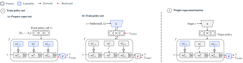
Fig. 1: Two-stage training of SWR. $f$, $g$, and $h$ are the feature extractor, the classifier, and the policy-net. Given a downstream task, $c$ is the target cost for $f$ after transfer learning, and $b$ is the binary policies for $L$ layers. \raisebox{-.9pt} {1}⃝ The policy-net is trained upon the super-net, which fine-tunes all the $L$ layers. \raisebox{-.9pt} {2}⃝ Layers are updated by weight reparametrization for a target policy.

2 Related works

Efficient transfer learning. Several studies, such as [3, 5, 6, 10], have suggested task-specific extra modules with pre-trained models. SpotTune [5] developed instance-specific dynamic gating to decide whether to use a fine-tuned or pre-trained block. Residual Adapter [3] suggested minimal extra channel-wise operations to adapt to a downstream task. Rep-Net [6] exploited an additional task-specific network parallel to its pre-trained backbone for intermediate feature reprogramming. In contrast, recently, TAPS [8] suggested a weight reparametrization with learnable scalar thresholding whether to use the reparametrization. While other methods [5, 3, 6] rely on extra task-specific modules, akin to our work, TAPS [8] utilized weight reparametrization. However, it is sensitive to hyperparameters and hence hard to optimize for target model efficiency. In contrast, we suggest a scalable policy network and an effective training process to achieve both target efficiency and reliably better performances.

3 Method

Problem definition. Given a pre-trained feature extractor, $f_{0}$, there are $T$ downstream tasks with corresponding training datasets, $D_{1},D_{2},\cdots,D_{T}$, where $D_{t}=\{x_{i},y_{i}\}_{i=1}^{N_{t}}$ with an example $x_{i}$ and its corresponding label $y_{i}$. Since the label sets of different tasks do not need to overlap, they usually have different class sets. By transfer learning to a task $t$, $f_{0}$ is updated to $f_{t}$, and task-specific classifier $g_{t}$ is newly learned. We aim to find $f_{t}$ and $g_{t}$ optimized to the corresponding objective and satisfy the constrained amount of updated weights for efficiency at multi-task transferring. Note that, in our work, $f_{t}$ contains the same number of parameters as $f_{0}$ (no complexities increase for a single task). We will omit $t$ for brevity.

3.1 Weight reparametrization & policy network

For a learnable layer $l\in\{1,\cdots,L\}$ of $f$, freezing the pre-trained weight $w^{0}_{l}$, SWR obtains the transferred weight $w_{l}$ by a learnable reparametrizing weight $w^{\prime}_{l}$ as [8]:

$$w_{l}=w^{0}_{l}+b_{l}w^{\prime}_{l},$$ (1)

where $b_{l}\in\{0,1\}$ is a policy that decides whether the $l$th layer weight is reparametrized (1) or not (0). $w^{\prime}_{l}$ is zero-initialized to let $w_{l}$ start from $w_{l}^{0}$. We reparametrize the learnable layers of policy 1 in $f$ except for batch normalization layers.

To obtain $b_{l}$’s, we design a policy network (policy-net) $h$, simply including three linear layers with ReLU in-between. The policy-net takes the target ratio of additional complexity to the original (refers to target cost, $c\in[0,1]$) as an input. The higher $c$, the more task-specific weights are allowed. Then, it yields $L$ 2-dimensional outputs, $\{h(c)_{l}\}_{l=1}^{L}$, where each $h(c)_{l}$’s first element , $h(c)_{l,1}$, is binarized as the policy by a threshold of 0.5 for each $l$.

During training, to make the layer-wise binary policy differentiable, we relax the discrete policies to continuous variables with hard Gumbel-Softmax [11], i.e., $b_{l}=\texttt{Gumbel}(h(c)_{l}/\tau)_{1}$, where $\tau$ is softmax temperature and 1 indicates the first element.

Note that the size of $w_{l}$ is as same as $w_{l}^{0}$, and the policy-net is not required after deployment; hence, there are no increased complexities of the transferred model in terms of the number of parameters and computations in a single downstream task. In multiple $T$ tasks, the increased parameters are only proportional to the amount of task-specific parts, which can be adjusted by $c$.

Transfer of batch normalization (BN). Previous works [3, 5, 6, 8] commonly update affine transformation parameters as well as running mean & variance in BN layers for each downstream task. However, their cost is not negligible in tiny networks. Therefore, inspired by [12], we only update the running mean & variance while freezing affine parameters to further reduce the number of updated parameters.

3.2 Two-stage training

We observed that co-optimizing $h$ and $\{w^{\prime}_{l}\}_{l=1}^{L}$ results in sub-optimal convergence. To prevent this, we suggest two-stage training. Fig. 1 depicts the overall procedure.

(1) Train policy-net with super-net. To get a reliable policy-net, we first learn the target downstream task using a super-net that transfers the pre-trained model by $w_{l}=w^{0}_{l}+w_{l}^{\prime}$, i.e., the policy is 1 for all $l$ in eq. (1). Hence, the policy-net is not considered here, and the super-net is learned with a target task loss $\mathcal{L}_{\mathrm{target}}$, e.g., conventional cross-entropy loss.

Next, while freezing the super-net, we train a policy-net $h$ varying the target cost input $c\sim\mathrm{Uniform}(0,1)$. We devise an additional loss term to learn the policy-net as

$$\mathcal{L}_{\mathrm{policy}}=|\{\sum_{l=1}^{L}{r_{l}\cdot\texttt{Softmax}(h(c)_{l}/\tau)_{1}}\}-c|,$$ (2)

where $r_{l}=\mathcal{N}(w_{l})/\sum^{L}_{i=1}{\mathcal{N}(w_{i})}$, a normalized layer-wise weighting according to $\mathcal{N}(w_{l})$, the number of parameters in $w_{l}$. The $r_{l}$ makes $\mathcal{L}_{\mathrm{policy}}$ considering the cost of layer $l$ based on $\mathcal{N}(w_{l})$. Here, we use Softmax instead of Gumbel-softmax in computing $\mathcal{L}_{\mathrm{policy}}$ (still use Gumbel-softmax in $\mathcal{L}_{\mathrm{target}}$). The total loss is $\mathcal{L}=\mathcal{L}_{\mathrm{target}}+\lambda\cdot\mathcal{L}_{\mathrm{policy}}$, where $\lambda$ is loss weighting hyperparameter.

(2) Weight reparametrization. The policy-net is now frozen and generates 0 or 1 binarized policies using the threshold of 0.5 as in Sec 3.1, given a target cost level $c$. Then, we only learn $w^{\prime}_{l}$’s whose corresponding policies are 1 with $\mathcal{L}_{\mathrm{target}}$.

4 Experiments

4.1 Experimental settings

Keyword spotting (KWS) detects pre-defined keywords in streaming audio [13]. We introduce a challenging transfer learning task that involves a multi-lingual pre-trained backbone being adapted to a monolingual KWS. We assess the averaged accuracy (Acc.$\uparrow$) with a 95% confidence interval. For efficiency, we report the total number of learnable parameters (#Param.$\downarrow$) compared to a single backbone and the number of multiplies (#Mult.$\downarrow$) for a single downstream task.

Datasets. We have created a transfer learning benchmark by combining two KWS datasets, Google speech commmands ver. 2 (GSC2) [14] for English and Mandarine Chinese Scripted Speech Corpus-Keyword Spotting (MC-KWS) [15]. GSC2 comprises 106K utterances from 2.6K speakers with each utterance being 1 sec. long and sampled at 16kHz. We have adapted the standard 12-way classification [13] for GSC2. MC-KWS contains 18 Chinese keywords from 37 speakers with each utterance being between [1.3, 6.2] sec. long and sampled at 48kHz. We have excluded the two English keywords, and out of the 18 remaining keywords, 7 are pairs of similar words and 4 are unpaired. We have followed the same preprocessing as in GSC [14, 13] and have also performed 12-way classification. To this end, we have assigned a keyword from each pair and randomly selected one of the unpaired keywords as a class, which we refer to as ‘unknown words’. The remaining 10 keywords constitute 10 known classes. We have also included the background noises from GSC2 as a separate class ‘silence’, with the length of 2.24 sec. For the train, validation and test sets, we have mapped 6.7k, 1.6k, 1.6k utterances, respectively from 25, 6, 6 speakers.

Table 1: Top-1 test accuracy and efficiency on GSC2 and MC-KWS for BCResNet-8 and Res15 backbones (Best: bold-faced, $2^{\textrm{nd}}$: underlined).

Method	Backbone	GSC2		MC-KWS	#Param.	#Mult.
Multi-lingual model	BCResNet-8	95.7 (1.6)		99.3 (0.4)	1x	1x
Fine-tuning All	BCResNet-8	98.5 (0.1)		99.8 (0.2)	3x	1x
SpotTune [5]	BCResNet-8	98.2 (0.3)		99.7 (0.4)	4.02x	1.79x
Adapter [3]	BCResNet-8	98.3 (0.2)		99.7 (0.2)	1.43x	1.53x
Rep-Net [6]	BCResNet-8	97.9 (0.5)		99.7 (0.2)	2.26x	2.15x
TAPS [8]	BCResNet-8	98.2 (0.2)		99.7 (0.1)	2.06x	1x
SWR, c=0.1	BCResNet-8	98.4 (0.2)		99.7 (0.0)	1.09x	1x
SWR, c=0.3	BCResNet-8	98.5 (0.1)		99.8 (0.2)	1.33x	1x
SWR, c=0.5	BCResNet-8	98.5 (0.1)		99.9 (0.1)	2.04x	1x
Multi-lingual model	Res15	95.4 (0.8)		96.2 (2.4)	1x	1x
Fine-tuning All	Res15	97.7 (0.2)		99.2 (0.2)	3x	1x
SpotTune [5]	Res15	96.3 (0.3)		94.6 (1.3)	4.08x	1.54x
Adapter [3]	Res15	97.5 (0.1)		98.7 (0.5)	1.22x	1.03x
Rep-Net [6]	Res15	97.5 (0.2)		98.7 (0.2)	1.86x	1.43x
TAPS [8]	Res15	97.4 (0.2)		98.6 (0.1)	2.00x	1x
SWR, c=0.1	Res15	97.6 (0.1)		99.0 (0.5)	1.08x	1x
SWR, c=0.3	Res15	97.6 (0.2)		99.3 (0.3)	1.54x	1x
SWR, c=0.5	Res15	97.7 (0.1)		99.3 (0.4)	2.00x	1x

Table 2: Ablation studies of SWR on BCResNet-8.

	c = 0.1			c = 0.3			c = 0.5
Method	GSC2	MC-KWS		GSC2	MC-KWS		GSC2	MC-KWS
Not staged (co-optimize)	97.2 (0.5)	97.5 (4.7)		97.9 (0.6)	99.6 (0.4)		98.1 (0.3)	99.6 (0.4)
SWR (Two-stage)	98.4 (0.2)	99.7(0.0)		98.5 (0.1)	99.8 (0.2)		98.5 (0.1)	99.9 (0.1)
+ BN-affine	98.3 (0.3)	99.8 (0.1)		98.3 (0.2)	99.9 (0.1)		98.5 (0.1)	99.9 (0.0)
+ Super-net weight	98.3 (0.2)	99.8 (0.1)		98.4 (0.1)	99.8 (0.1)		98.5 (0.1)	99.8 (0.2)

Implementation. We employ two tiny backbones: Broadcasting residual networks (BCResNet-8) [13] and Res15 [16]. BCResNet-8 is SOTA on GSC2 through its efficient design with 321k parameters utilizing broadcasted residual learning. Res15 was designed for KWS task based on conventional residual networks [17]. For each, we adopted the data preprocessing and augmentation outlined in the literature and followed the training scheme for a pre-trained backbone, ‘Multi-lingual model’. The pre-training involved classification of combined classes in both GSC and MC-KWS.

We fine-tune 30 epochs for weight reparametrization of our SWR using $\lambda$ of 1 and Adam optimizer with a learning rate initialized by {1e-3, 5e-4} and cosine-annealed without weight decay. Next, we schedule the (Gumbel) Softmax temperature by cosine annealing from 2 to 0.5 [11]. In the second stage of SWR, we do zero initialization for $w^{\prime}_{l}$’s instead of using the super-net for fair comparisons regarding training cost. Finally, we select the transferred model at the last epoch for evaluation.

4.2 Results

Table 1 demonstrates the KWS results. We compare our SWR with the recent efficient transfer learning methods, Spottune [5], Residual Adapter [3], Rep-Net [6], and TAPS [8]. We follow their official implementations for transfer learning on KWS. The multi-lingual pre-trained backbone shows lower accuracy than a model entirely fine-tuned in a single language (‘Fine-tuning All’) due to the differences in English and Chinese characteristics [18, 19]. Our SWR outperforms the baselines [5, 3, 6, 8], and even surpasses ‘Fine-tuning All’ which updates the entire layers. Notably, SWR achieves comparable or even better performance than the baselines, merely with the target cost of 0.1, which requires the smallest extra costs, i.e., zero computation and less than 10% of the number of parameters.

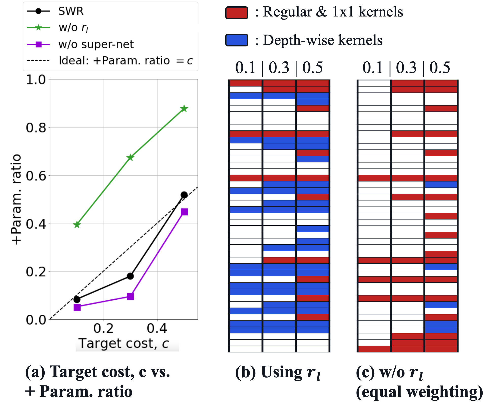
Fig. 2: Controllability of SWR on GSC2. (a) Target cost vs. actual increased parameters (+Param. ratio). (b) & (c) Resulting policy for 43 convolution layers for different costs {0.1, 0.3, 0.5} (layers go deeper from top to bottom).

4.3 Analysis

In this section, we analyze SWR on BCResNet-8.

Two-stage training. To see the benefit of the two-stage training, we co-optimize the policy-net $h$ and the reparametrizing weights $w^{\prime}_{l}$’s, ‘Not staged.’ The first two rows of Table 2 compare it with our complete method, SWR. In all $c$, SWR outperforms ‘Not staged.’ Hence, the two-stage training is more favorable for optimizing both $h$ and $w^{\prime}_{l}$’s.

Affine paramters in BN & Super-net weight. Comparing the second and third rows of Table 2, we see that updating affine parameters of BN layers does not guarantee better transfer to downstream tasks but rather inevitably degrades the efficiency in SWR. Contrarily, TAPS [8] specifies both layers and affine parameters to each task. Nevertheless, it performs less than the proposed SWR (Table 1). It means that our policy-net finds more informative layers to be updated. Next, the last row in Table 2 shows that using super-net, which is fine-tuned with policies of all 1, as initialization of $w_{l}^{\prime}$ in the second stage does not guarantee better performance.

Efficacy of super-net in cost controllablity. SWR provides the high-performing transferred model under an efficiency constraint, the target cost $c$. In Fig. 2(a), we plot the ratio of the increased parameters to the pre-trained model in a transferred model varying $c$, ablating SWR. Hence, the more it matches the ideal (black-dashed), the better controllability. We can see that SWR (black-circle) is closer to the ideal than ‘w/o super-net’ (purple-square) in all $c$. Compared to SWR, ‘w/o super-net’ yields undesirable results: less parameters, but degraded performances by 0.1% for $c$ of 0.1 and 0.3, respectively. From this, we found that the strategy of super-net-based policy-net learning is essential.

Learned policy. BCResNet-8 includes a single regular convolution (conv) and seperated convs where each consists of depth-wise (temporal and frequency) and 1x1 convs [13]. Usually, depth-wise kernels have fewer parameters than the others, hence less weighted by $r_{l}$ in eq. (2). Fig. 2 shows obtained policies over 43 layers in BCResNet-8 on transfer learning to GSC2 depending on $r_{l}$. The colored boxes denotes weight-reparametrized layers by policies of 1. Red and blue boxes indicate {regular conv, 1x1} and depth-wise kernels, respectively. Without $r_{l}$ (equal weighting), the policy-net is more likely to select heavy computations (more red boxes in Fig. 2(c)), resulting in green-star in Fig. 2(a). On the other hand, with $r_{l}$, the policy-net prefers the depth-wise kernels to the 1x1 and regular conv kernels as in Fig. 2(b). Then, we can obtain better parameter efficiency (black-circle in Fig. 2(a)).

Table 3: Top-1 test accuracy using ResNet50 on ImageNet-to-Sketch benchmark (Best: bold-faced, $2^{\textrm{nd}}$: underlined). *: reproduced numbers, ^†: results from [8]

Method	Flowers	WikiArt	Sketch	Cars	CUB	#Param.
Fine-tuning All†	95.7	78.0	81.8	91.2	83.6	6x
Fine-tuning Classifier†	89.1	61.7	65.9	55.5	63.5	1x
SpotTune [5]	96.3	75.8	80.2	92.4	84.0	7x
Rep-Net [6]	96.7	76.4*	80.3*	88.7*	80.3	7.85x
TAPS [8]	96.7	76.9	80.7	89.8	82.7	4.12x
SWR, c=0.1	96.0	75.6	79.6	91.2	83.7	1.83x
SWR, c=0.3	96.8	76.0	80.3	91.3	84.9	2.42x
SWR, c=0.5	97.0	77.0	80.7	92.2	85.2	3.40x

4.4 Extend to larger backbone

Benchmark: ImageNet-to-Sketch. To verify the effectiveness of our SWR in a larger backbone, we apply SWR in a transfer learning benchmark ImageNet-to-Sketch [9], where five downstream tasks are Flowers [20], CUBS [21], Cars [22], Sketch [23], and WikiArts [24], based on a ImageNet [25] pre-trained model . In this benchmark, the resnet-50 [17] is the standard backbone. We follow the settings of the recent related literature and released source code [6, 8]: we fine-tune for 50 epochs for SWR using $\lambda=3$, SGD optimizer with a learning rate of {5e-3, 1e-2, 2e-2} and cosine annealed with weight decay of {1e-4, 0}, and label smoothing of 0.3.

Results. We compare the proposed SWR with the recent methods [5, 6, 8] in Table 3. Our SWR achieves par or surpasses the SOTA accuracy on four downstream tasks while using fewer additional parameters, 3.40x. Only in the task, Cars, SWR achieves the second best, 92.2, which is lower than 92.4 of SpotTune, which uses double the additional number of parameters. The results show the feasibility of our SWR for a larger backbone, e.g., resnet-50, at a different domain, Image recognition.

5 Conclusions

In this work, we proposes a novel efficient transfer learning called Scalable Weight Reparametrization (SWR). SWR learns reparametrization of pre-trained weights with the policy network, which determines which layers to reparametrize under an efficiency constraint. We also proposed a two-stage learning process for a reliable training of both reparametrization parameters and the policy network. Regarding accuracy and efficiency, SWR achieved the SOTA in KWS with tiny backbones and successfully extended to a larger backbone in image classification.

References

- [1] Jacob Devlin, Ming-Wei Chang, Kenton Lee, and Kristina Toutanova, “BERT: pre-training of deep bidirectional transformers for language understanding,” in NAACL-HLT (1), 2019.
- [2] Alexei Baevski, Yuhao Zhou, Abdelrahman Mohamed, and Michael Auli, “wav2vec 2.0: A framework for self-supervised learning of speech representations,” in NeurIPS, 2020.
- [3] Neil Houlsby, Andrei Giurgiu, Stanislaw Jastrzebski, Bruna Morrone, Quentin de Laroussilhe, Andrea Gesmundo, Mona Attariyan, and Sylvain Gelly, “Parameter-efficient transfer learning for NLP,” in ICML, 2019.
- [4] Ken Chatfield, Karen Simonyan, Andrea Vedaldi, and Andrew Zisserman, “Return of the devil in the details: Delving deep into convolutional nets,” in BMVC, 2014.
- [5] Yunhui Guo, Honghui Shi, Abhishek Kumar, Kristen Grauman, Tajana Rosing, and Rogério Schmidt Feris, “Spottune: Transfer learning through adaptive fine-tuning,” in CVPR, 2019.
- [6] Li Yang, Adnan Siraj Rakin, and Deliang Fan, “Rep-net: Efficient on-device learning via feature reprogramming,” in CVPR, 2022.
- [7] Gamaleldin F. Elsayed, Ian J. Goodfellow, and Jascha Sohl-Dickstein, “Adversarial reprogramming of neural networks,” in ICLR, 2019.
- [8] Matthew Wallingford, Hao Li, Alessandro Achille, Avinash Ravichandran, Charless C. Fowlkes, Rahul Bhotika, and Stefano Soatto, “Task adaptive parameter sharing for multi-task learning,” CoRR, vol. abs/2203.16708, 2022.
- [9] Arun Mallya, Dillon Davis, and Svetlana Lazebnik, “Piggyback: Adapting a single network to multiple tasks by learning to mask weights,” in ECCV, 2018.
- [10] Anjuli Kannan, Arindrima Datta, Tara N. Sainath, Eugene Weinstein, Bhuvana Ramabhadran, Yonghui Wu, Ankur Bapna, Zhifeng Chen, and Seungji Lee, “Large-scale multilingual speech recognition with a streaming end-to-end model,” in INTERSPEECH, 2019.
- [11] Eric Jang, Shixiang Gu, and Ben Poole, “Categorical reparameterization with gumbel-softmax,” in ICLR, 2017.
- [12] Ximei Wang, Ying Jin, Mingsheng Long, Jianmin Wang, and Michael I. Jordan, “Transferable normalization: Towards improving transferability of deep neural networks,” in NeurIPS, 2019.
- [13] Byeonggeun Kim, Simyung Chang, Jinkyu Lee, and Dooyong Sung, “Broadcasted residual learning for efficient keyword spotting,” in INTERSPEECH, 2021.
- [14] Pete Warden, “Speech commands: A dataset for limited-vocabulary speech recognition,” arXiv preprint arXiv:1804.03209, 2018.
- [15] “Mandarin chinese scripted speech corpus,” https://magichub.com/datasets/mandarin-chinese-scripted-speech-corpus-keyword-spotting-2/.
- [16] Raphael Tang and Jimmy Lin, “Deep residual learning for small-footprint keyword spotting,” in ICASSP, 2018.
- [17] Kaiming He, Xiangyu Zhang, Shaoqing Ren, and Jian Sun, “Deep residual learning for image recognition,” in CVPR, 2016.
- [18] Yizhou Lu, Mingkun Huang, Hao Li, Jiaqi Guo, and Yanmin Qian, “Bi-encoder transformer network for mandarin-english code-switching speech recognition using mixture of experts,” in INTERSPEECH, 2020.
- [19] Ngoc-Quan Pham, Tuan-Nam Nguyen, Sebastian Stüker, and Alex Waibel, “Efficient weight factorization for multilingual speech recognition,” in INTERSPEECH, 2021.
- [20] Maria-Elena Nilsback and Andrew Zisserman, “Automated flower classification over a large number of classes,” in ICVGIP, 2008.
- [21] Catherine Wah, Steve Branson, Peter Welinder, Pietro Perona, and Serge Belongie, “The caltech-ucsd birds-200-2011 dataset,” Technical Report CNS-TR-2011-001, California Institute of Technology, 2011.
- [22] Jonathan Krause, Michael Stark, Jia Deng, and Li Fei-Fei, “3d object representations for fine-grained categorization,” in ICCV Workshops, 2013.
- [23] Mathias Eitz, James Hays, and Marc Alexa, “How do humans sketch objects?,” ACM Trans. Graph., vol. 31, no. 4, pp. 44:1–44:10, 2012.
- [24] Babak Saleh and Ahmed M. Elgammal, “Large-scale classification of fine-art paintings: Learning the right metric on the right feature,” CoRR, vol. abs/1505.00855, 2015.
- [25] Jia Deng, Wei Dong, Richard Socher, Li-Jia Li, Kai Li, and Li Fei-Fei, “Imagenet: A large-scale hierarchical image database,” in CVPR, 2009.