Technical constraints on interstellar interferometry and spatially resolving the pulsar magnetosphere

Abstract

Scintillation of pulsar radio signals caused by the interstellar medium can in principle be used for interstellar interferometry. Changes of the dynamic spectra as a function of pulsar longitude were in the past interpreted as having spatially resolved the pulsar magnetosphere. Guided by this prospect we used VLBI observations of PSR B1237+25 with the Arecibo and Green Bank radio telescopes at 324 MHz and analyzed such scintillation at separate longitudes of the pulse profile. We found that the fringe phase characteristics of the visibility function changed quasi-sinusoidally as a function of longitude. Also, the dynamic spectra from each of the telescopes shifted in frequency as a function of longitude. Similar effects were found for PSR B1133+16. However, we show that these effects are not signatures of having resolved the pulsar magnetosphere. Instead the changes can be related to the effect of low-level digitizing of the pulsar signal. After correcting for these effects the frequency shifts largely disappeared. Residual effects may be partly due to feed polarization impurities. Upper limits for the pulse emission altitudes of PSR B1237+25 would likely be well below the pulsar light cylinder radius. In view of our analysis we think that observations with the intent of spatially resolving the pulsar magnetosphere need to be critically evaluated in terms of these constraints on interstellar interferometry.

1 Introduction

Scattering of radio waves by inhomogeneities of the interstellar plasma causes angular broadening of the source image, distortion of radio spectra, and scintillation. Refractive scintillation are slow and occur on time scales of $t_{\mathrm{ref}}$ and diffractive scintillation are fast and occur on time scales of $t_{\mathrm{dif}}$, with corresponding spatial scales of $\rho_{\mathrm{ref}}$ and $\rho_{\mathrm{dif}}$. Fluctuations in the density of free electrons in the interstellar plasma produce variations in the index of refraction. Pulsars observed through such a medium produce a diffractive pattern in the plane of the observer. The medium can be seen as a lens or an interferometer with an extremely large baseline and therefore, depending on the distance of the medium from the pulsar, providing extremely high spatial resolution. Using interstellar interferometry it is therefore possible in principle to probe the sizes of pulse emission regions, as well as their separations and relative motions with a spatial resolution in most cases much better than a light cylinder radius, $r_{\mathrm{LC}}=cP/2\pi$, with $c$ the speed of light and $P$ the pulsar period. Early discussions and studies were reported by Scheuer (1968) and Lovelace (1970). The theory of interstellar plasma lensing was further developed by, e.g., Rickett (1977); Cordes et al. (1986); Gwinn et al. (1998).

First attempts to resolve the pulsar magnetosphere were made by Backer (1975) and Cordes et al. (1983) by comparing scintillation patterns of different pulse profile components. No evidence of independent scintillation was found resulting in upper limits of the corresponding emission regions of as small as $1.2r_{\mathrm{LC}}$ or $3\times 10^{4}$ km for PSR B0823+26 and $1\times 10^{4}$ km or, with particular assumptions, even $1\times 10^{3}$ km for PSR B0525+21, respectively.

First phase sensitive attempts of resolving the pulsar magnetosphere were done by Bartel et al. (1985) with VLBI and gating. These authors discussed the effects of polarization impurities of the feeds on measurements of visibility phase as a function of pulse longitude of PSR B0329+54 and therefore on the separation of emission regions. They derived stringent limits for the feeds so that the bias due to the changing polarisation characteristics across the pulsar’s profile would be reduced for sensitive fringe phase measurements along pulsar longitude. Again, no evidence for having resolved the pulsar magnetosphere was found.

The first apparently clear evidence for having resolved with interstellar interferometry the magnetosphere of a pulsar was reported by Wolszczan & Cordes (1987) by having made use of occasionally occurring refractive scintillation. A strong refraction event can split the image into two or multiple subimages. Wolszczan & Cordes (1987) observed periodic structure in the dynamic spectrum of PSR B1237+25 with the Arecibo telescope (AR) at 430 MHz. They interpreted that structure as an interference pattern formed when two radiation beams having different paths through the interstellar medium (ISM) intersect in the observer plane. They detected an asymmetric non-monotonic smooth fringe phase variation of the periodic structure in the dynamic spectra as a function of pulse longitude and estimated a typical transverse separation between the emission regions of $\sim 10^{3}$ km for a screen at half distance between the pulsar and Earth. For a magnetic dipole field such separation would place the emission regions at $r_{\mathrm{LC}}$. Only a screen much closer to the pulsar would lower the emission altitude substantially. The authors also discussed an alternative of a very distorted dipole field for a reduced altitude of the emission region.

Very similar results were reported for PSR B1133+16 by Gupta et al. (1999) using the Ooty radio telescope at 327 MHz. They also used multiple imaging during a refractive event and again found a non-monotonic fringe phase variations across the pulse profile. They inferred a minimum separation of the emission regions of the leading and trailing parts of a pulse of $3\times 10^{7}$ m corresponding to a minimum emission height of $\geq 2.6\times 10^{3}$ km.

Further apparently successful attempts to spatially resolve the emission region were reported by several authors. Smirnova & Shishov (1989) analyzed dynamic diffractive scintillation spectra as a function of longitude and found through cross-correlation analysis lags in time and frequency indicating separations of the corresponding emission regions of $3\times 10^{2}\,$km, which for a dipole magnetic field corresponds to an emission height of $0.08r_{\mathrm{LC}}$. In a similar analysis using however the cross-correlation peak degradation as a function of longitude separation, Smirnova (1992) and Smirnova et al. (1996) found for some other pulsars, including PSR B1237+25, in contrast, emission heights close to $r_{\mathrm{LC}}$. Similarly, focusing on giant pulses of the Crab pulsar, Main et al. (2021) found with diffractive scintillation for the main pulse and interpulse sizes and separations of approximately $r_{\mathrm{LC}}$, although it should be noted that in this case $r_{\mathrm{LC}}$ is with  1,600 km relatively small.

On the other hand, Johnson et al. (2012) used diffractive scintillation of the Vela pulsar and measured the size of the emitter to be $<4$ km and its height to be $<3.4\times 10^{2}$ km, much smaller than $r_{\mathrm{LC}}$. Also Pen et al. (2014) following Brisken et al. (2010) reduced VLBI observations of PSR B0834+06 with primarily AR and the Green Bank Telescope (GB) with 4-level digitization at 327 MHz and then used VLBI imaging of its scattering speckle pattern to measure the changing phase response on the scattering screen as a function of pulse longitude. The authors found a phase change of $\sim 0.01$ rad over an $\sim 18$ ms longitude range of the pulse profile. They interpreted it as a deflection or an apparent motion of only 18 km or $\sim 1000\,\text{km\,s}^{-1}$ of a small emission region at an altitude of a few hundred km, effectively performing high-precision astrometry with an angular resolution of 50 picoarcseconds.

Summarizing, although there have been efforts for almost half a century to resolve the pulsar magnetosphere with sometimes apparently extremely high spatial resolution, no consistent picture as to the magnitude of the displacements of the emission regions along the pulse profile or the emissions’ altitude, near the pulsar or close to $r_{\mathrm{LC}}$, has yet emerged.

Inspired by these results from interstellar interferometry we focused on the multicomponent pulsar B1237+25 and used VLBI observations with the AR and GB telescopes as well as the respective observations with the single antennas. Our goal was to probe the scintillation properties and determine any changes as a function of pulsar longitude to derive the corresponding emission regions’ separations or their upper limits. In Section 2 we describe our observations and the primary reduction of our data. In Section 3 we show the visibility phases from the VLBI observations as they change as a function of pulse longitude and compare the results with the corresponding frequency shifts of the dynamic spectra for each of the single telescopes. In Sections 4 and 5 we explain why our changes in the scintillation properties are not indicative of having resolved the pulsar magnetosphere but in contrast can be largely if not completely attributed to effects of low-level digitization of the data. In Section 6 we critically discuss our findings in view of previous reports of having resolved the magnetosphere, emphasize the technical constraints that need to be considered for interstellar interferometry and draw conclusions about the physics of the emission regions and the distance of the scattering screen for PSR B1237+25. In Section 7 we give a summary of our results and our conclusions.

2 Observations and primary data reduction

We made VLBI observations of PSR B1237+25 with AR and GB at 324 MHz with a bandwidth, $B=16$ MHz at right (RCP) and left-circular (LCP) polarization. The observations were made in the context of the Radioastron space-VLBI science program AO-5. We used two observing sessions separated by two months for the PSR B1237+25, and one observing session for the PSR B1133+16, each 2 h long. General information about the sessions is given in Table 1. All sessions consisted of six 1160 s long recording scans separated by 30 s gaps. During each scan, 840 pulsar periods with $P=1.38$ s were used for our analysis of data for PSR B1237+25. The data were processed at Astro Space Center with the ASC software correlator (Likhachev et al., 2017) with gating and incoherent dedispersion applied. We used 512 channels at the correlator, providing a frequency resolution of 31.25 kHz.

Table 1: List of observations.

PSR	Date	Time		Stations	$\Delta f_{1/e}$	$t_{\mathrm{dif}}$	$\Delta\tau_{1/2}$
	(yyyy mm dd)	(hh:mm -hh:mm)			(MHz)	(s)	(ns)
(1)	(2)	(3)		(4)	(5)	(6)	(7)
B1237+25	2017 12 22	10:00 - 12:00		AR, GB, WB	1.70-4.40	345±20	65± 5
B1237+25	2018 02 26	05:30 - 07:30		AR, GB	0.71-1.22	250±10	260±10
B1133+16	2018 12 17	09:00 - 11:00		AR, GB, WB	1.50-2.30	80.4±4	320±20

Note. — Columns are as follows: (1) Pulsar observed. (2) Date of observations related to observing codes rags29c, rags29j, and raks24e for the first, second and third epoch, respectively. (3) Time span of observations for six scans. Each scan is 1160 s long which corresponds for PSR B1237+25 to 840 pulsar periods and for PSR B1133+16 to 976 pulsar periods. (4) Radio antennas scheduled for the observations, AR – Arecibo, GB – Robert C. Byrd Green Bank Telescope, WB – Westerbork. We report here only results for AR and GB in VLBI mode and single antenna mode. (5) Decorrelation bandwidth as half-width at 1/e of the maximum of the frequency section of the 2-dim autocorrelation function (ACF) at zero time lag measured with AR for window, $\text{w}_{4}$, of the pulse profile (see Figure  1). The ranges refer to the minimum and maximum values for the six scans for each of the two epochs. (6) Diffractive scintillation time. (7) Half-width at half maximum of the visibility magnitude obtained in sub-window $\text{w}_{1}$ for one scan. Uncertainties in (6) and (7) are statistical standard errors.

First, we computed the average pulse profile and dynamic spectrum for AR for each of the two observing sessions. The pulse profiles are shown in Figures  1a and 1b. The width of the pulse window is $\sim 65$ ms, corresponding to a longitude range of $\sim 16$ deg. Note, the slight false decrease of intensity at the leading and trailing part of the profile which we will discuss in Section 5. The dynamic spectra are shown in Figures 1c and 1d. The spectra are similar to what would be expected under regular, diffractive, scattering conditions. No quasi-periodic modulation as a consequence of multiple imaging due to refraction is observed.

Second, we divided the pulse window into nine sub-windows, w_k, with $0\leq k\leq 8$, each $\sim 7$ ms wide (see Figures 1a and 1b). We also selected three off-pulse sub-windows, w_k, with $9\leq k\leq 11$, of the same duration. Then we computed with the correlator for each window the complex cross-spectrum for the baseline AR-GB, $S^{AR-GB}_{k}(f_{i},t_{j})$, and the auto-spectrum, $S_{k}(f_{i},t_{j})$ (dynamic spectrum), for each of the two radio telescopes. Each dynamic spectrum consists of $N_{\mathrm{f}}N_{\mathrm{t}}$ values, with $1\leq i\leq N_{\mathrm{f}}$ and $1\leq j\leq N_{\mathrm{t}}$ where $N_{\mathrm{f}}$ is the number of frequency channels covering the frequency range in the bandpass from 316 to 332 MHz, and $N_{\mathrm{t}}$ the number of spectra in a given set of observations. We corrected the dynamic spectrum $S_{k}(f_{i},t_{j})$ in each sub-window, w_k, for the background baseline as follows:

$$S_{k}(f_{i},t_{j})=S^{\mathrm{on}}_{k}(f_{i},t_{j})-S^{\mathrm{off}}(f_{i},t_{j}).$$ (1)

Here, $S^{\mathrm{on}}_{k}$ is the spectrum obtained in each of the sub-windows, $\text{w}_{0}$ to $\text{w}_{8}$, and $S^{\mathrm{off}}$ is the spectrum average over the off-pulse windows, $\text{w}_{9}$ to $\text{w}_{11}$. The individual spectra were averaged over four pulse periods to smooth out the intensity fluctuations from pulse to pulse, reducing $N_{\mathrm{t}}$ to 210 but keeping $N_{\mathrm{f}}=512$.

Third, we computed the two-dimensional cross-correlation functions between the dynamic spectra of each of the sub-windows and the dynamic spectrum of the sub-window in the center of the pulse, w₄, which served as a reference.

$$CCF_{4k}(\Delta f,\Delta t)={\frac{1}{(N_{\mathrm{f}}-i)(N_{\mathrm{t}}-j)}}\sum_{i=0}^{N_{\mathrm{f}}-i}\sum_{j=0}^{N_{\mathrm{t}}-j}\Delta S_{4}(f_{i},t_{j})\Delta S_{k}(f_{i}+\Delta f,t_{j}+\Delta t).$$ (2)

Here $\Delta f={\frac{B}{N_{\mathrm{f}}}}i$ and $\Delta t=4Pj$ are frequency and time lags, and $\Delta S_{k}(f,t)=S_{k}(f,t)-\langle S_{k}(f,t)\rangle$ with

$$\langle S_{k}(f,t)\rangle={\frac{1}{N_{\mathrm{f}}N_{\mathrm{t}}}}\sum_{i=1}^{N_{\mathrm{f}}}\sum_{j=1}^{N_{\mathrm{t}}}S_{k}(f_{i},t_{j})\,.$$ (3)

After the primary data reduction we proceeded to the main analysis.

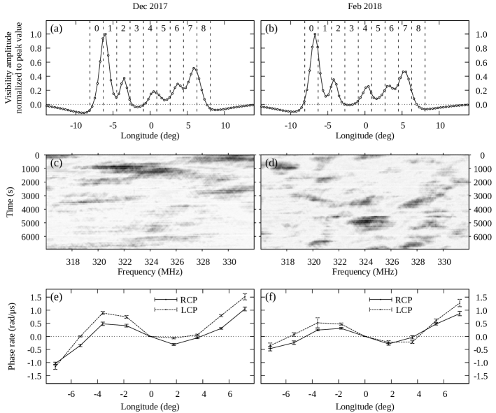
Figure 1: Pulse profiles of PSR B1237+25 observed at RCP (panels a, b), dynamic spectra of diffractive scintillation at RCP (panels c, d), and rate of change of the visibility phases as a function of pulsar longitude for both senses of polarization (panels e, f), each averaged over six scans. Left and right panel columns are for our two observing epochs, 2017 December 22 and 2018 February 26, respectively. Pulse profiles in (a, b) are computed as the visibility magnitude obtained by the correlator at zero baseline for AR with the off-pulse levels subtracted. The vertical dashed lines indicate the nine on-pulse sub-windows, $\text{w}_{0}$ to $\text{w}_{8}$, used as gates for the correlation and for our analysis. Dynamic spectra in (c, d) are the averages for AR over the full on-pulse windows and shown on normalized linear gray-scale. The black and white regions represent the maxima and minima of the power density, respectively. Phase rates, in (e, f), are the derivatives of the AR-GB VLBI visibility phases from strong pulses with respect to delay, $\frac{d(\varphi_{k}-\varphi_{4})}{d\tau}$ for the nine pulse windows with $0\leq k\leq 8$. Uncertainties are standard errors. They were derived from the $1\sigma$ uncertainty from the least-squares fit of the phase rates in the approximately $\pm$ 125 ns central delay region for each of the six scans and then divided by $\sqrt{6}$.

3 Phase and frequency shifts as a function of pulsar longitude

3.1 Phase shifts of the VLBI visibility functions

For every single pulse and every sub-window, with $0\leq k\leq 11$, we computed the complex visibility function $V_{k}(\tau)$ as the inverse Fourier transform of $S^{AR-GB}_{k}(f)$ with the sampling interval in interferometer delay, $\tau$, being equal to 31.25 ns. We used only visibilities for the AR-GB baselines. As an example we give the average of the visibility function magnitude for one scan and for window $\text{w}_{1}$ in Figure 2.

Figure 2: Upper panel: Average AR-GB visibility magnitude as a function of interferometer delay for PSR B1237+25 obtained in sub-window $\text{w}_{1}$ for one scan (10:00) on 2017 December 22. The solid line shows a Lorenzian, fit to the data. It has a half-width-at-half-maximum (HWHM) of 65 ns. Lower panel: Corresponding average differences of the visibility phases between the leading ($\text{w}_{0}$) and trailing ($\text{w}_{8}$) sub-windows relative to the phases for sub-window, $\text{w}_{4}$. The phases were corrected for $2\pi$-ambiguities. Only RCP pulses with the highest SNR were used. The tilted lines are least-squares fits to the aligned phases in the central region of the visibility magnitude curve. Uncertainties are smaller or approximately equal to the symbol sizes. Phases outside the central region have much larger errors.

Then we investigated the phases, $\phi_{k}$ of $V_{k}(\tau)$ relative to $\phi_{4}$ of $V_{4}(\tau)$ as a function of longitude. We selected only strong pulses with the signal-to-noise ratio (SNR) in both the selected sub-window, $\text{w}_{k}$, and sub-window $\text{w}_{4}$ being $>$5 with respect to the off-pulse window, $\text{w}_{11}$. For these pulses we computed for each sub-window in the pulse profile the phase relative to the phase in sub-window, $\text{w}_{4}$, ($\varphi_{k}-\varphi_{4})$. We analyzed data from six scans and obtained for every scan and every window in general several hundreds of phase differences from our strong pulses.

As an example, we present the average phase differences for the leading ($\varphi_{0}-\varphi_{4})$ and the trailing ($\varphi_{8}-\varphi_{4})$ sub-windows as a function of $\tau$ in Figure 2. In the approximately $\pm 125\,\text{ns}$ delay window the curves of phase differences can be approximated by straight lines with a fitted slope of $\frac{d(\varphi_{k}-\varphi_{4})}{d\tau}$ for k=0 and 8. As can be seen in Figure 2, the slopes are very different for the leading and trailing windows relative to window 4. In general, these slopes vary across the pulse window. In Figures 1e and 1f we plot the values of the varying slopes and their standard errors from the fit for each sub-window with respect to the value for window, $\text{w}_{4}$, for the two polarizations and the two days of observations.

The variations are smooth, highly significant and appear to be quasi-sinusoidal with an upward trend along longitude. The patterns in Figures 1e and 1f are very similar for the two polarizations and for the two days. We note that our pattern of the VLBI phase rate versus pulse longitude is also very similar to the comparable pattern of phase versus longitude presented for PSR B1237+25 by Wolszczan & Cordes (1987) and for PSR B1133+16 by Gupta et al. (1999). However, we will show that in our case this pattern is not an indication of having resolved the pulsar magnetosphere. The variation of the derivative of phase along longitude can be converted to a frequency shift through the relation $|\Delta f|=\frac{1}{2\pi}|\frac{d\varphi}{d\tau}|$. From, e.g., Figure 1e we obtain the total change of the LCP phase derivative across the profile from $\text{w}_{0}$ to $\text{w}_{8}$ of $\sim 2.65\,\text{rad}/\mu s$ which, with the shifting property of the Fourier transform, corresponds to a shift in frequency of the dynamic spectra to lower frequencies by an amount of $\sim$-420 kHz.

3.2 Frequency shifts of the dynamic spectra

We can also see the frequency shift in our dynamic spectra as a function of longitude for each of the two telescopes separately. In Figure 3 we show on the left side the dynamic spectra in windows $\text{w}_{0}$ (top panel) and $\text{w}_{8}$ (bottom panel). The latter one is slightly but clearly shifted toward lower frequencies with respect to the former.

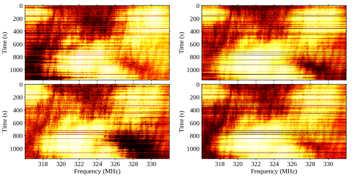
Figure 3: The dynamic spectra in longitude windows w₀ (top) and w₈ (bottom) observed at AR in LCP on 2017 December 22 (scan 1). The left panels show the dynamic spectra before correction. A shift of about 1 MHz toward lower frequencies from w₀ to w₈ can be seen. The right panels show the corresponding spectra after correction as described in Section 4. The spectrum in w₀ is copied from the left side for better comparison. The spectrum in w₈ shows that the frequency shift has largely disappeared. For the difference of the time-averaged spectra and a discussion, see Subsection 4.1.

A more detailed presentation of the frequency shift is obtained with $CCF_{4k}(\Delta f,\Delta t$), of the dynamic spectra magnitudes $S(f,t)$. First, we determined the decorrelation bandwidth, $\Delta f_{1/e}$ as the lag at 1/e of the maximum from the frequency cross-section of the autocorrelation function, $CCF_{44}$, of the dynamic spectra in $\text{w}_{4}$. We list the range of values for the six scans for each of the two observing epochs in Table 1 and list the individual values in Table 2.

Second, we determined the frequency shift of the dynamic spectra in each of the sub-windows relative to the spectrum in $\text{w}_{4}$. For this purpose we used the frequency sections of $CCF_{4k}(\Delta f,\Delta t$) for $\Delta t=0$. As an example we take the dynamic spectra from $\text{w}_{0}$ and $\text{w}_{8}$ from Figure 3 (left panels) and cross-correlate them with respect to that of $\text{w}_{4}$. The corresponding functions $CCF_{4k}$ with k=0 and 8 are plotted for AR and GB in Figure 4.

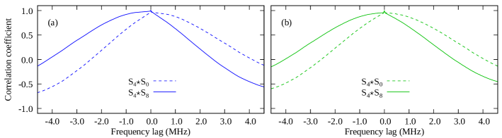
Figure 4: Examples of frequency sections of the two-dimensional CCF($\Delta f,\Delta t$) functions for $\Delta t=0$ of dynamic spectra as a function of frequency lag, $\Delta f$. Panels (a) and (b) correspond to AR and GB, respectively. The CCF’s are computed for two pairs of dynamic spectra, one corresponding to the leading and the middle window ($\text{w}_{0}$-$\text{w}_{4}$, solid curves) and the other to the trailing and the middle window ($\text{w}_{8}$-$\text{w}_{4}$, dashed curves). The CCFs were normalized to have equal values at zero lag. LCP data were used from scan 1 at epoch 2017 December 22.

A shift of spectra in $\text{w}_{8}$ to lower frequencies with respect to spectra in $\text{w}_{0}$ is clearly visible.

For an accurate determination of the frequency shift we accounted for the asymmetry of the functions by fitting to them the function, $Y(x)$, with $x=\Delta f$ and $x_{0}$ as the frequency shift with

$$Y(x)=A\exp{{\left(-\frac{|x-x_{0}|}{B}^{\alpha}\right)}}+C+D(x-x_{0}).$$ (4)

Here, $C$, compensates for a possible baseline offset, D, accounts for the asymmetry of the CCF and, $\alpha$, for the shape of the CCF. We determined the frequency shifts, $x_{0}$, for the dynamic spectra in each window relative to that in $\text{w}_{4}$ for each of the six scans and each of the observing epochs. The fitted values of $\alpha$ are in the range of 1.5 to 1.8. The frequency shift values, $x_{0}$, correspond to shifts of the spectra from the leading part of the pulse profile in $\text{w}_{0}$ to the trailing part in $\text{w}_{8}$.

We plot the frequency shifts with dashed lines for AR and GB for each of the scans for the first epoch in Figure  5 and plot the averages from all six scans in Figure  6. The frequency shifts for our second epoch could be better inspected by averaging over all six scans and the two polarizations and telescopes. For comparison we plot these averages in the right panel in the same Figure.

Figure  6 shows that the quasi-sinusoidal modulation of the frequency shift as a function of longitude is very similar for AR and GB on 2017 December 22. It is also similar to the shape of the modulation on 2018 February 26. However, the modulation amplitude is about 20 times smaller. We found that this decrease in amplitude is related to a decrease in $\Delta f_{1/e}$.

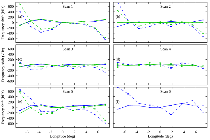
Figure 5: Frequency shifts of dynamic spectra in $\text{w}_{0}$ to $\text{w}_{8}$ relative to spectrum in $\text{w}_{4}$. Panels (a-g) present results for the six scans obtained in LCP at AR (blue lines) and GB (green lines) on 2017 December 22. For scan 6 the GB data were not usable and are omitted. Each scan is 840 pulse periods long. Dashed lines correspond to original, uncorrected frequency shifts. Solid lines correspond to remaining relatively small frequency shifts after correction for distortion discussed in subsection  4.1. Uncertainties are 1$\sigma$ statistical standard errors determined from the fit of eq. 4.

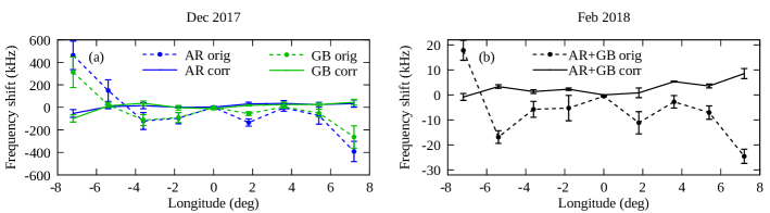
Figure 6: Left panel: The averages of the frequency shifts for 2017 December 22 for windows $\text{w}_{0}$ to $\text{w}_{8}$ relative to $\text{w}_{4}$ for the six scans in Figure  5. Right panel: The corresponding frequency shifts for 2018 February 26 averaged over all scans, the two polarizations and the two telescopes. Uncertainties are standard errors.

In Table  2 we list the magnitudes of the maximum frequency shifts as a function of $\Delta f_{1/e}$ for each of the six scans of the two epochs and plot them in Figure  7. A weighted least-squares fit of the maximum frequency shift, $M_{f-shift}$, to a polynomial, $M_{f-shift}=A(\frac{\Delta f_{1/e}}{MHz})^{b}$, gives A=0.04$\pm$0.01 MHz and b=2.7$\pm$0.2 with scaled uncertainties so that Chi-square per degree of freedom, $\chi^{2}_{\nu}=1$.

Table 2: Decorrelation bandwidth and freq. shift

Date	Scan	$\Delta f_{1/e}$	Max. freq. shift
(yyyy mm dd)	(number)	(MHz)	(MHz)
2017 12 22	1	3.57±1.80	1.05±0.01
	2	3.53±1.76	1.30±0.03
	3	2.50±1.10	0.37±0.01
	4	1.70±0.60	0.22±0.02
	5	3.50±1.60	1.25±0.03
	6	4.40±2.50	0.95±0.03
2018 02 26	1	1.15±0.26	0.044 ±0.008
	2	0.70 ±0.14	0.015±0.005
	3	1.02±0.26	0.042±0.007
	4	1.03 ±0.26	0.068 ±0.007
	5	1.20 ±0.30	0.058±0.005
	6	1.23±0.32	0.052±0.005

Note. — The decorrelation bandwidth, $\Delta f_{1/e}$ and the magnitude of the maximum frequency shift, with standard errors, along pulse longitude for scans 1 to 6 for each of the two observing dates. For the computation of the error of $\Delta f_{1/e}$, see Bartel et al. (2022). For errors of the frequency shift, see caption of Figure  5

Figure 7: Maximum frequency difference observed in AR LCP dynamic spectra in $\text{w}_{8}$ relative to $\text{w}_{0}$ as a function of decorrelation bandwidth, $\Delta f_{1/e}$, taken from Table 2. The shift is to lower frequencies for the dynamic spectra from the leading part of the pulse profile in $\text{w}_{8}$ to the trailing part in $\text{w}_{0}$. The data from Feb. 2018 February 26 are all in the lower left corner.

4 Cause and Characterization of distortions

4.1 Effect similar to dispersion delay

What could be the cause of the observed phase rate and frequency shift changing across the pulse profile? Earlier, Bartel et al. (1985) considered the varying polarisation as a function of pulse longitude combined with polarisation impurities of the feed that could lead to interferometer phase changes across the pulse profile. Here we will show that low-level digitization effects lead to the distortions as a function of longitude that can be best illustrated by considering the dispersion delay of the pulsar signal across the receiver bandpass combined with the diffraction features of the dynamic spectrum before dedispersion.

In Figure 8 (left upper panel) we present the dynamic spectra, S₀ and S₈, for AR of Figure 3 (left panels) for the leading and trailing windows respectively but averaged in time. For comparison we also show the corresponding spectra for GB (right upper panel). For each of AR and GB the S₀ spectra of the leading window $\text{w}_{0}$ appear to be shifted toward higher frequencies compared to the S₈ spectra of the trailing window $\text{w}_{8}$.

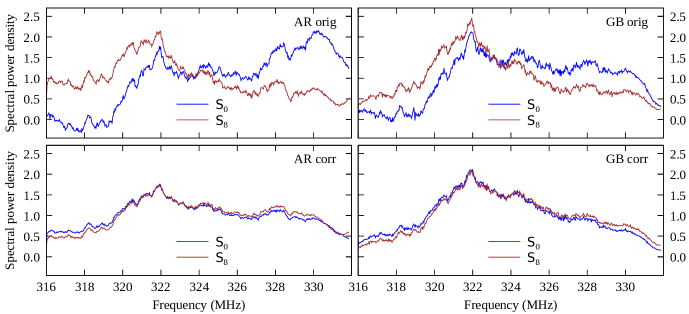
Figure 8: Comparison of AR and GB time-averaged LCP spectra for leading ($S_{0}$) and trailing ($S_{8}$) windows, each with the spectrum for the off-pulse subtracted. Upper panels show spectra before correction and lower panels after correction. The spectra correspond to scan 1 of 1160 s duration on 2017 December 22. The spectra were normalized so that the frequency-averaged power spectral density $\bar{S}=1$.

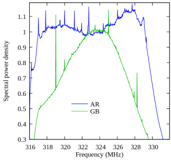
Figure 9: Bandpasses for AR and GB from average spectra of off-pulse longitude windows, $\text{w}_{9}$ to $w_{11}$, from scan 1 on 2017 December 22.

These characteristics are similar to what could be expected for a pulsar signal sweeping down in frequency with different pulse components illuminating scintles in the spectrum at different frequencies.

The average profile of PSR B1237+25 consists of 5 components as it is shown in Figure 1. With a dispersion measure, $DM=9.3~{}\text{cm}^{-3}~{}\text{pc}$, it takes about 36 ms for the pulsar signal to sweep across the 16 MHz band from 332 to 316 MHz. The spectrum $S_{0}$ corresponds to the case where the strong leading component comes to the high frequency part of the bandpass dominating the illumination and amplification of the diffraction features in the averaged dynamic spectrum between 332 and 328 MHz, thus causing a false visible shift of the spectrum to higher frequencies. The weight of the illumination and the amplification changes and becomes more balanced while the pulse travels through the bandpass, minimizing the frequency shift in the central region of our profile. However, the shift continues clearly further to lower frequencies when the strong trailing component of the pulse profile dominates the illumination and amplification of the dynamic spectrum between 324 and 318 MHz causing a false visible shift of $S_{8}$ to lower frequencies. This effect is already indicated in Figure  3 (left panels) for the dynamic spectra of $\text{w}_{0}$ and $\text{w}_{8}$ but can be more clearly seen in Figure 8.

Also, the effect is particularly strong for AR for which the bandpass is almost flat across the 16 MHz bandwidth (see, Figure 9). In contrast, the bandpass for GB attenuates the high and low frequencies of the full bandwidth which weakens the effect of the illuminations of the diffraction features at the filter ends. The result is a smaller frequency shift which can be seen in Figures 4, 6, and 8.

4.2 Effect of signal digitization

The ASC correlator corrects for the dispersion delay by composing the full spectrum for a given time from a sample of delayed spectra. In our case we used 1000 time bins per pulsar period, giving us 1000 corresponding spectra with 512 channels each. With this number of channels our correlator produces spectra every $32~{}\mu$s. Each such spectrum is subject to a redistribution of harmonics between corresponding bin spectra. Thus, for every pulsar period, the spectrum at every bin will be corrected for the dispersion delay. Our processing system is described by Likhachev et al. (2017). Nevertheless we still have, for spectra at different longitudes, distortions similar to those expected due to the influence of the dispersion delay.

The reason for the distortions can be traced back to the effects of digitizing a non-stationary stochastic signal like the pulsar signals probed in this paper (Jenet & Anderson, 1998). For one-bit digitizing (clipping) where negative values are recorded as -1, and positive values as +1 the signal variance $\sigma^{2}=1.0$. For a signal with frequency components, $1\leq k\leq N_{f}$, up to a maximum of $N_{f}$ the variance of a signal is related to the spectral power density, $s_{k}$, by $\sigma^{2}=2\sum_{k=1}^{N_{f}}s_{k}$. If we assume that there is an excess of spectral power density at relatively high frequencies beyond component $a$, with $k>a$, then there will be a false deficiency of spectral power density at relatively low frequencies, $k<a$. Let us assume that the current output spectrum from the correlator has such high frequency excess because the beginning of the pulse reached the receiver band. This output single spectrum would be redistributed between time bins with inadequate values, namely, underestimated low frequency values of the spectral power density would go to the preceding time bins causing a false decrease of total power. On the other hand, the high frequency portion of the spectrum at the leading longitude of the average profile would be overestimated. Thus, the one-bit digitizing acts like a non-compensated dispersion delay.

The same effect can be seen under saturation conditions for two-bit (four level) digitizing used at both AR and GB. Under normal conditions with no saturation of the signal four values are utilized for such digitizing, -3, -1, +1, and +3. A transition level, $s_{0}$, between $\pm 1$ and $\pm 3$ values must be close to $\sigma$, with $s_{0}=0.995\sigma$ (Thompson et al., 2017). An automatic gain control system (AGC) is used at each of our telescopes to keep the system at such a level during VLBI observing session. The AGC will compensate progressive slow signal variations caused by a change in elevation of the source or weather condition. For pulsar observations the AGC would not work correctly due to its inertia. Therefore, we switched off the AGC system in our observations. With the AGC switched off, the digitizer was saturated for strong pulses at such sensitive radio telescopes as AR and GB. Under saturation conditions the digitizer acts like a one-bit sampler with only values of $\pm 3$, generating false spectral distortions. One can see this effect in the average profiles shown in Figure 1 most clearly where the intensity dips below the baseline on each side of the profile. Such digitizing also acts like a non-compensated dispersion delay. For multilevel digitization of pulsar signals the non-compensated dispersion delay is less likely and decreases with the number of digitization levels.

4.3 Distortion observations of other pulsars

Can the effect of distortion also be found in other pulsars? As an example we present in Figure 10 results for PSR B1133+16, with an average profile with two components, $P=1.19$ s, $DM=4.84$ cm^-3 pc, and $\Delta f_{1/e}=1.8$ MHz. We analyzed the average profile and the phase rate between visibility functions for different longitude windows, as described in Section 3 and plot the results in Figure  10.

Figure 10: Top: Average profile of PSR B1133+16 at LCP obtained at AR for scan 1 on 2018 December 17. Bottom: Phase rates as the derivatives of the AR-GB VLBI visibility phases with respect to delay as a function of pulse longitude for the same observing scan. Plots are based on original, uncorrected data. For more information, compare with Figure 1.

As for PSR B1237+25 the average pulse profile is distorted with intensity decreases at both sides of the profile, and the phase rates vary non-monotonically as a function of pulse longitude. The maximum difference is $\sim$1.2 rad/$\mu$s which corresponds to a frequency shift of $\sim$190 kHz. The shift is again from higher frequencies at the leading part of the pulse profile to lower frequencies at the trailing part. However, the magnitude of the shift for this pulsar is much larger than what would be expected from Figure  7 for PSR B1237+25. Clearly, the maximum frequency shift across the pulse profile depends also on the pulsar under study.

In general we think that this distortion effect can be observed in any pulsar independent of the complexity of its profile. However while the frequency shift across a profile with two or more components is rather modulated, this frequency shift would likely be much smoother and generally monotonic for a single component profile.

5 Significant reduction of distortion

As was indicated in the previous section, the observed distortions as a function of pulsar longitude can be explained in terms of effects of dispersion and low-level digitization. Since all VLBI observations of the RadioAstron mission were archived, we accessed the original VLBI data and applied the corrections of 2-bit sampling as outlined by Jenet & Anderson (1998).

To give a short summary, the method of correction is based on using Gaussian statistics of samples of records of the original VLBI data before dedispersion. Without correction the average pulse profile displays characteristic intensity distortions including the dips before and after the profile (see Figure 11) similar to the dips shown in (Jenet & Anderson, 1998) for the Vela pulsar under study by them. For the correction we first analyzed a very small part of the recorded signal and calculated the portion of samples $\psi$ corresponding to +/- 1 values. If there were no digitization distortions, this portion would be equal to 2/3 and corresponded to a correct threshold level $H$ of $\pm 1\sigma$ of the recorded signal. On strong pulses the statistics would be different, and with the calculated current portion $\psi$ the true value of the threshold, $\pm H$ of the distorted digitized data could be estimated for Gaussian distribution. The next step is to calculate the corrected values of the samples as a mean for Gaussian distribution between zero and $\pm H$ instead of $\pm 1$ and as a mean between $\pm H$ and $\pm\infty$ instead of $\pm 3$. Thus, we corrected every sample using moving average for bit statistics. For another description of the application of digitization correction, see van Straten & Bailes (2011).

We also coherently dedispersed the data (see, Hankins, 1974) for improvement over incoherent dedispersion although without any apparent effect on the correction itself. For further details of our data reduction and correction process, see Girin et al. (2023). In Figure  11 we also show the corrected dedispersed average profile for easy comparison with the uncorrected profile. It can be clearly seen that the intensity distortions including the dips outside the profile have disappeared.

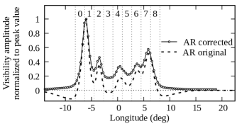
Figure 11: Average profile of PSR B1237+25 for the original data obtained at AR for scan 1 on 2017 December 12 (copied from Figure 1) and the profile after correction. Note, the intensity dips on both sides of the profile have disappeared.

The dips of intensity below the off-pulse level on each side of the profile have disappeared. As for the dynamic spectra in $\text{w}_{0}$ and $\text{w}_{8}$, we show in Figure 3 that after correction the frequency shift has also largely disappeared. The details of the frequency shift as a function of longitude after correction are displayed in Figure 5. The corrected frequency shifts (solid lines) for both AR and GB are significantly reduced in amplitude and are almost constant along longitude in comparison to the original data (dashed lines). The same characteristics can also be found in the averaged spectra in Figure 6.

Further insight can be derived from the time-averaged spectra in Figure 8. Close inspection shows that the narrow spectral features in the original data are not shifted along longitude. Instead the weight within the spectra is shifted. For the leading part of the pulse the spectrum, $S_{0}$, has on average more power at higher frequencies which shifts to lower frequencies in the spectrum for the trailing part of the profile, $S_{8}$ (see also interpretation in subsection 4.1). Again, the corrected spectra show almost no differences between those of the leading and trailing pulse parts.

6 Discussion

Our observations can be compared with those of PSRs B1237+25 at 430 MHz at AR by Wolszczan & Cordes (1987) and B1133+16 at 327 MHz at Ooty by Gupta et al. (1999). These authors observed that the dynamic spectra as a function of longitude were shifted non-monotonically from high frequencies at the leading part of the pulse profile to low frequencies at the trailing part within their receiver bandpasses.

We found a similar shift of the spectra from high to low frequencies in our VLBI observations with AR and GB as well as in observations with each single telescope. In particular, Wolszczan & Cordes (1987) reported for PSR B1237+25 a frequency shift of 39 kHz across the pulse profile. The decorrelation bandwidth for their two days of observations was 442 and 615 kHz. Although their observing frequency of 430 MHz was somewhat higher than ours, their observed maximum frequency shift is comparable with our prediction of  10 kHz for 327 MHz from Figure 7 which further indicates that the nature of their longitudinal frequency shift of the dynamic spectra is similar to ours.

An important aspect is that both groups used, as we did, low-level digitizers, at AR 3-level (Wolszczan & Cordes, 1987) and at Ooty 1-bit samplers (Bhat et al., 1999). Through our analysis we can now trace our longitudinal frequency shift back to digitization effects. In view of interstellar interferometry we expect that most if not all pulsar observations with low-level digitization, technically or because of saturation, can be affected by longitudinal distortion if the effects discussed above are not addressed in detail.

Despite having largely corrected for the low-level digitizing effects for PSR B1237+25, some apparently significant residuals remain in our data. Are these due to small technical effects that still remain uncorrected or do they have an astrophysical origin and indicate a marginal resolution of the magnetosphere?

The cause is not clear. Perhaps our estimated uncertainties are too small and the differences from zero frequency shifts are not significant. The correction process itself may not be completely effective for our data. Lastly, the polarization impurities of the telescope feeds, although not subject of this paper, need to be considered when computing the limiting effect of the changing polarization characteristics along pulsar longitude on the phase and frequency shifts (see, Bartel et al., 1985). In this respect, the frequency shifts along longitude in RCP and LCP for AR and GB (see, Figure 1) are of interest. While there is fair consistency between the curves, there are also slight differences between the RCP and LCP curves that vary with longitude differently for AR and GB. Such an effect may be conceivable for different polarization impurities of the feeds at the two telescopes.

If however, the discrepancies have an astrophysical cause, then it is possible to elaborate on the emission separations and corresponding altitudes for a pulsar magnetic dipole field. In this context it is interesting to note that, as displayed in Figure 6, after correction the differences in the frequency shifts between the leading and trailing parts of the profiles where the shifts are largest, averaged for AR and GB, are about 100 kHz on Dec. 2017 but only 10 kHz on February 2018. In relative terms the remaining shifts are about 15 and 25$\%$ of the uncorrected shifts, respectively. If the remaining frequency shifts of the corrected data had an astrophysical origin, then the shifts would be expected to be of the same magnitude on both days. That they were not and instead have similar portions of the shifts of their uncorrected data suggests that a large part of the residual shifts are still due to remaining uncorrected technical effects as discussed above. Any residual frequency shift variations due to having resolved the magnetosphere must therefore be smaller than even a portion of the largest shift variations of the corrected data from February 2018 in Figure 6.

Wolszczan & Cordes (1987) estimated for PSR B1237+25 emission separations of $\sim$1,000 km and respective altitudes of $r_{\mathrm{LC}}$. If we take for our data an upper limit of any astrophysics related freqency shift of, say $10\%$ of the uncorrected frequency shifts, and apply this correction factor to the data of Wolszczan & Cordes (1987), then their estimate of the emission altitude would be only $0.1r_{\mathrm{LC}}$, eliminating any need for a very distorted dipole field or a screen very close to the pulsar. However, as for deriving estimates directly from our observations, their computations for refractive scintillation would not be directly applicable to our data with diffractive scintillation.

Diffractive scintillation was studied by Cordes et al. (1983) and applied to a correlation analysis of dynamic spectra of PSRs B0525+21 and B1133+16 with AR at 430 MHz. No correlation degradation or significant frequency shifts beyond the spectral resolution of 1.2 and 40 kHz for the two pulsars respectively, were found for the spectra of the leading and trailing parts of the pulse profiles. With their model they derived emission separations of also $\sim 1,000$ km and emission altitudes of $<0.06r_{\mathrm{LC}}$ and $<0.53r_{\mathrm{LC}}$. From these comparisons our upper limit of only a couple of kHz of astrophysics related frequency shift would suggest that the emission altitude is also well below $r_{\mathrm{LC}}$.

In general, we think that the constraints discussed here need to be taken into account for observations with the goal of resolving spatially the pulsar magnetosphere. With appropriate considerations a distortion-less use of interstellar interferometry could likely be achieved.

7 Summary and Conclusions

Here we summarize our observations and give our conclusions.

1. Inspired by earlier reports of having resolved the magnetosphere of pulsars with interstellar interferometry, we used VLBI observations of PSR B1237+25 conducted with AR and GB at 324 MHz and analyzed the interferometry as well as the single telescope data. All observations were done in the context of the RadioAstron space-VLBI mission.

2. During a time of diffractive scintillation, the dynamic spectra changed as a function of pulsar longitude with the spectrum of the leading part at higher frequencies shifting for the trailing part to lower frequencies.

3. In VLBI data as well as single telescope data the frequency shift displayed a non-monotonic pattern as a function of pulsar longitude. Although the patterns were largely similar for AR and GB, differences could be due to differences in the bandpasses.

4. The maximum frequency shift, between the spectra of the leading and trailing parts of the pulse profile is a steep function of decorrelation bandwidth.

5. The integrated pulse profile showed characteristic deficiencies in intensity at both sides of the profile.

6. Similar distortions of the scintillation spectra as a function of longitude and of the pulse profile were found for PSR B1133+16.

7. Despite having observed characteristic phase and frequency shifts in scintillation spectra as a function of pulsar longitude, we do not contribute the shifts to having resolved the pulsar magnetosphere.

8. We attribute the distortions and frequency shifts of the longitude-dependent dynamic spectra mostly to uncorrected low-level digitizing of the data.

9. With the data corrected (see, Jenet & Anderson, 1998), the non-monotonic frequency shift pattern of the dynamic spectra along pulse longitude largely disappeared.

10. Small remaining distortions could perhaps partly be caused by polarization impurities of the feeds.

11. Upper limits of any astrophysics related frequency shifts would suggest that the altitude of emission regions for PSR B1237+25 is well below $r_{\mathrm{LC}}$.

12. In view of our analysis we think that observations with the intend to resolve the pulsar magnetosphere need to be critically evaluated in terms of these constraints on interstellar interferometry.

References

- Backer (1975) Backer, D. C. 1975, A&A, 43, 395
- Bartel et al. (2022) Bartel, N., Burgin, M. S., Fadeev, E. N., et al. 2022, ApJ, 941, 112, doi: 10.3847/1538-4357/ac9eae
- Bartel et al. (1985) Bartel, N., Ratner, M. I., Shapiro, I. I., et al. 1985, AJ, 90, 2532, doi: 10.1086/113958
- Bhat et al. (1999) Bhat, N. D. R., Rao, A. P., & Gupta, Y. 1999, ApJS, 121, 483, doi: 10.1086/313198
- Brisken et al. (2010) Brisken, W. F., Macquart, J. P., Gao, J. J., et al. 2010, ApJ, 708, 232, doi: 10.1088/0004-637X/708/1/232
- Cordes et al. (1986) Cordes, J. M., Pidwerbetsky, A., & Lovelace, R. V. E. 1986, ApJ, 310, 737, doi: 10.1086/164728
- Cordes et al. (1983) Cordes, J. M., Weisberg, J. M., & Boriakoff, V. 1983, ApJ, 268, 370, doi: 10.1086/160961
- Girin et al. (2023) Girin, I. A., Likhachev, S. F., Rudnitskiy, A. G., et al. 2023, Processing system for coherent dedispersion of pulsar emission. https://arxiv.org/abs/2303.17280
- Gupta et al. (1999) Gupta, Y., Bhat, N. D. R., & Rao, A. P. 1999, ApJ, 520, 173, doi: 10.1086/307442
- Gwinn et al. (1998) Gwinn, C. R., Britton, M. C., Reynolds, J. E., et al. 1998, ApJ, 505, 928, doi: 10.1086/306178
- Hankins (1974) Hankins, T. H. 1974, A&AS, 15, 363
- Jenet & Anderson (1998) Jenet, F. A., & Anderson, S. B. 1998, PASP, 110, 1467, doi: 10.1086/316273
- Johnson et al. (2012) Johnson, M. D., Gwinn, C. R., & Demorest, P. 2012, ApJ, 758, 8, doi: 10.1088/0004-637X/758/1/8
- Likhachev et al. (2017) Likhachev, S. F., Kostenko, V. I., Girin, I. A., et al. 2017, Journal of Astronomical Instrumentation, 6, 1750004, doi: 10.1142/S2251171717500040
- Lovelace (1970) Lovelace, R. V. E. 1970, PhD thesis, -
- Main et al. (2021) Main, R., Lin, R., van Kerkwijk, M. H., et al. 2021, ApJ, 915, 65, doi: 10.3847/1538-4357/ac01c6
- Pen et al. (2014) Pen, U.-L., Macquart, J.-P., Deller, A. T., & Brisken, W. 2014, MNRAS, 440, L36, doi: 10.1093/mnrasl/slu010
- Rickett (1977) Rickett, B. J. 1977, ARA&A, 15, 479, doi: 10.1146/annurev.aa.15.090177.002403
- Scheuer (1968) Scheuer, P. A. G. 1968, Nature, 218, 920, doi: 10.1038/218920a0
- Smirnova (1992) Smirnova, T. V. 1992, Soviet Astronomy Letters, 18, 392
- Smirnova & Shishov (1989) Smirnova, T. V., & Shishov, V. I. 1989, Soviet Astronomy Letters, 15, 191
- Smirnova et al. (1996) Smirnova, T. V., Shishov, V. I., & Malofeev, V. M. 1996, ApJ, 462, 289, doi: 10.1086/177150
- Thompson et al. (2017) Thompson, A. R., Moran, J. M., & Swenson, George W., J. 2017, Interferometry and Synthesis in Radio Astronomy, 3rd Edition (Springer, Cham), doi: 10.1007/978-3-319-44431-4
- van Straten & Bailes (2011) van Straten, W., & Bailes, M. 2011, PASA, 28, 1, doi: 10.1071/AS10021
- Wolszczan & Cordes (1987) Wolszczan, A., & Cordes, J. M. 1987, ApJ, 320, L35, doi: 10.1086/184972