Modelling the braking “index” of isolated pulsars

Abstract

An isolated pulsar is a rotating neutron star possessing a high magnetic dipole moment that generally makes a finite angle with its rotation axis. As a consequence, the emission of magnetic dipole radiation (MDR) continuously takes away its rotational energy. This process leads to a time decreasing angular velocity of the star that is usually quantified in terms of its braking index. While this simple mechanism is indeed the main reason for the spin evolution of isolated pulsars, it may not be the only cause of this effect. Most of young isolated pulsars present braking index values that are consistently lower than that given by the MDR model. Working in the weak field (Newtonian) limit, we take in the present work a step forward in describing the evolution of such a system by allowing the star’s shape to wobble around an ellipsoidal configuration as a backreaction effect produced by the MDR emission. It is assumed that an internal damping of the oscillations occurs, thus introducing another form of energy loss in the system, and this phenomenon may be related to the deviation of the braking index from the pure MDR model predictions. Numerical calculations suggest that the average braking index for typical isolated pulsars can be thus simply explained.

I Introduction

The identification of isolated pulsars hewish1967 with rotating neutron stars presenting a high surface magnetic field was suggested long ago gold1968 , where predictions about their spin evolution were also anticipated. Shortly thereafter, the pulsar detected in the Crab nebula was measured richards1968 to slow down. It is by now well understood that the main cause of the spin evolution of pulsars is the loss of energy due to the emission of magnetic dipole radiation pacini1967 ; pacini1968 ; gunn1969 . As this radiation carries angular momentum, the star angular velocity decreases with time, leading to a slowing-down behavior that has been detected for the last 50 years.

When only this source is considered, the rate at which the rotational energy is radiated away from the pulsar is described by the well known equation of dipole radiation shapiro ; pacini1968 ; gunn1969 (in units where $c=1=\mu_{0}$, where $\mu_{0}$ the magnetic vacuum permeability)

$$\dot{E}=-\frac{2}{3}\mu^{2}\Omega^{4}\sin^{2}\!\alpha,$$ (1)

where $\Omega=2\pi\nu$ is the angular velocity of the star, with $\nu$ its rotation frequency, while $\mu$ is the magnitude of its magnetic dipole moment $\bm{\mu}$, making an angle $\alpha$ with its rotation axes, determined by $\bm{\Omega}$, as illustrated in Fig. 1. In Eq. (1) and in what follows, a dot over a physical quantity represents its time derivative. In our system of units, the amplitude $\mu$ of the magnetic dipole moment is related with that of the magnetic field $B$ through $\mu=\frac{1}{2}BR^{3}$.

The relationship between $\dot{E}$, $\Omega$, and the moment of inertia $I$ of the star is given by the torque equation $\dot{\Omega}=(I\Omega)^{-1}\dot{E}$, leading to $\dot{\Omega}=-\beta\;\Omega^{3}$, where we have defined

$$\beta\doteq\frac{2}{3}\frac{\mu^{2}}{I}\sin^{2}\alpha.$$ (2)

More generally, the different causes behind the slowing-down phenomenon can be encapsulated by the power law formula goldwire1969 $\dot{\Omega}=-K\Omega^{n}$, where $n$ is the so-called braking “index” of the pulsar. It is usually defined as if $K$ were constant, namely

$$n\doteq\frac{\Omega\ddot{\Omega}}{\dot{\Omega}^{2}},$$ (3)

and is actually constant only for constant $K$.

In the oversimplified model above with constant magnetic dipole moment, angle and moment of inertia, i.e. assuming $K_{\text{dipole}}=\beta$ constant, one naturally gets $n=3$, while a model based only on gravitational waves radiation ostriker1969 leads to $n=5$.

Precise measurements of the braking index of several isolated pulsars have revealed values that are consistently different than that predicted on a purely magnetic dipole model with constant $K$ (see for instance the review in Ref. lyne2015 ). Consequences of assuming $K$ as time dependent function Blandford1988 has been examined magalhaes2012 ; lyne2015 , and depending on the way $K$ evolves in time, the braking index can be $n\not=3$. Furthermore, assuming hamil2015 $I=I[\Omega(t)]$ only in the magnetic dipole model is not enough to explain the present observational data for the known isolated pulsar. However, it was reported hamil2016 that assuming a time dependent inclination angle $\alpha=\alpha(t)$ would be a possible way to explain the phenomenon.

All the models described above are based on the simplifying assumption that the kinetic energy $E_{\textsc{k}}$ of the body is only due to its rigid rotation, i.e., $E_{\textsc{k}}=\frac{1}{2}I\Omega^{2}$. However, a neutron star cannot be strictly considered as rigid and even though the rotation is very slow from the point of view of relativistic effects, with typical surface velocities of the order of $v\simeq(10^{-4}-10^{-2})c$, the shape should be allowed to depend on time as this rotation may naturally induce a flattening of the poles. In such a scenario, the kinetic energy acquires new contributions that need to be taken into account.

It is the purpose of the present work to introduce a more complete description taking into account the variation of the internal potential energy of a self-gravitating body Lucas2015 . In particular, we explore the consequences of allowing the star shape to evolve in time, under its coupling with the rotation of the body. It is assumed that energy can be lost in this process, a phenomenon that could be relevant in the explanation of the measured slowing-down of isolated pulsars. Embedding our model in a general relativistic context goes beyond the scope of this work, and as we consider the quasi-rigid rotation of the star, we restrict attention to the Newtonian weak field limit; given the slow velocities involved, we expect this approximation to be meaningful.

In the next section, the basic assumptions of the model are described and the coupled system of nonlinear differential equations governing the evolution of the star are derived. The results of our numerical analysis are presented in Sec. III, where some suggestive solutions are studied. In particular, we show that a pulsar evolution with $n<3$ can easily be reproduced. A comparison between our results and the available data describing the behavior of the Crab pulsar is given in Sec. IV, before a few final and concluding remarks in Sec. V.

II The model

Suppose the star is described as a mass distribution that is slightly deformed compared to a spherical body and is rotating around the $z$-axis with time-dependent angular velocity $\Omega(t)$. We assume the volume of the star to be that of the non rotating sphere $\frac{4}{3}\pi R^{3}$, its actual shape being ellipsoidal with two equal semi-axes in the $(x,y)-$plane slightly larger than the sphere radius, i.e. $(1+b)R$ (see Fig. 1). Even for the large velocities involved in a rotating neutron star, we do not expect large deviations from sphericity and thus demand that $b\ll 1$. As a result, the volume of the ellipsoid matches that of the sphere to second order in $b$ provided the semi-axis in the direction of rotation is $(1-2b)R$. An arbitrary element of mass $\text{d}m$ in the body will thus be described by the set $\bm{R}^{\prime}=\{X^{\prime},Y^{\prime},Z^{\prime}\}$ such that

$$\left(\frac{X^{\prime}}{1+b}\right)^{2}+\left(\frac{Y^{\prime}}{1+b}\right)^{2}+\left(\frac{Z^{\prime}}{1-2b}\right)^{2}\leq R^{2}.$$

As discussed in the introduction, we expect the quantity $b$ may not necessarily be constant, so we anticipate that $b=b(t)$. It is convenient to use a coordinate system related to that of the embedding sphere, i.e., the set $\{x,y,z\}$ such that $x^{2}+y^{2}+z^{2}=r^{2}$, with $r\leq R$. That is, we implement the coordinate transformation $X^{\prime}=(1+b)x$, $Y^{\prime}=(1+b)y$ and $Z^{\prime}=(1-2b)z$. The volume element, as expected, is $\text{d}V=\text{d}X^{\prime}\text{d}Y^{\prime}\text{d}Z^{\prime}=\text{d}x\text{d}y\text{d}z+\mathcal{O}(b^{2})$.

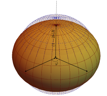
Figure 1: The pulsar geometric configuration: the neutron star is rotating with angular velocity $\Omega(t)=\dot{\varphi}$ around the $z$ axis while its magnetic axis is inclined by an angle $\alpha$ leading to precession of the field lines. The rotation induces a deviation from sphericity so the original sphere of radius $R$ (dashed grid) turns into an ellipsoid whose semi-axes are depend on time through the function $b(t)$ related to the ellipticity.

Let us implement a rotation $\mathcal{R}_{\bm{\hat{z}}}(\varphi)$ to the body about the $z$-axis by an angle $\varphi$. The position $\bm{r}^{\prime}$ of the mass element $\text{d}m$ is then given by the rotation applied to its location $\bm{R}^{\prime}$, i.e. $\bm{r}^{\prime}(\varphi,b)=\mathcal{R}_{\bm{\hat{z}}}(\varphi)\cdot\bm{R}^{\prime}$. One therefore gets

$$\bm{r}^{\prime}=\underbrace{\left(\begin{matrix}\cos\varphi&\sin\varphi&0\cr-\sin\varphi&\cos\varphi&0\cr 0&0&1\end{matrix}\right)}_{\mathcal{R}_{\bm{\hat{z}}}(\varphi)}\underbrace{\left(\begin{matrix}1+b&0&0\cr 0&1+b&0\cr 0&0&1-2b\end{matrix}\right)\left(\begin{matrix}x\cr y\cr z\end{matrix}\right)}_{\bm{R}^{\prime}},$$ (4)

whose modulus we denote by $r^{\prime}$.

Since we consider a pulsar, i.e. a rotating neutron star, one now needs to assume from that point on that both the rotation angle $\varphi$ and the flattening of the poles depend on time. The absolute velocity, $v=\|\text{d}\bm{r}^{\prime}/\text{d}t\|$, of each mass element in such system is given by

$$v=\sqrt{(x^{2}+y^{2}+4z^{2}){\dot{b}}^{2}+(x^{2}+y^{2})\Omega^{2}(1+b)^{2}},$$ (5)

where $\Omega=\dot{\varphi}$ is the angular velocity of $\text{d}m$ around the $z$-axis. The kinetic energy $E_{\textsc{k}}$ of the star is obtained by integrating $\frac{1}{2}v^{2}\text{d}m$ over the whole body volume, leading to

$$E_{\textsc{k}} = \frac{1}{2}\dot{b}^{2}\int_{V}(x^{2}+y^{2}+4z^{2})\rho(r)\text{d}V$$ (6)

$$+\frac{1}{2}\Omega^{2}(1+b)^{2}\int_{V}(x^{2}+y^{2})\rho(r)\text{d}V,$$

where $\rho(r)$ is the mass-density function that is supposed to depend only on the distance to the origin.

The moment of inertia $I$ of the neutron star, seen as an idealized spherical mass distribution rotating about the $z$-axis, is defined by

$$I\doteq\int\left(x^{2}+y^{2}\right)\rho(r)\text{d}V,$$

which, because of the spherical symmetry, is also expressible as

$$I=2\int\rho x^{2}\text{d}V=2\int\rho y^{2}dV=2\int\rho z^{2}\text{d}V.$$ (7)

For the spherical approximation, it reads $I=\frac{2}{5}MR^{2}$, so that Eq. (2) then implies $\beta\approx 5B^{2}R^{4}/(12M)$.

The kinetic energy now reads

$$E_{\textsc{k}}=\frac{3}{2}I\dot{b}^{2}+\frac{1}{2}I(1+2b)\Omega^{2}+\mathcal{O}(b^{2}).$$ (8)

As the system evolves, the body will be allowed to oscillate. Its potential energy $E_{\textsc{p}}$ can be expanded about $b=0$, as

$$E_{\textsc{p}} \approx E_{p}(0)+\frac{1}{2}\kappa b^{2},$$ (9)

where we have used that the potential energy is minimized for the spherical configuration, so that $\left(\partial E_{\textsc{p}}/\partial b\right)_{b=0}=0$. In Eq. (9), we noted the elastic constant as

$$\kappa=\left(\frac{\partial^{2}E_{\textsc{p}}}{\partial b^{2}}\right)_{b=0}=3I\gamma,$$ (10)

thereby defining the coefficient $\gamma$. The leading contribution to the elastic constant can be obtained by assuming the spherical approximation, which leads to $\kappa\approx 24GM^{2}/(5R)$, such that $\gamma\approx 4GM/R^{3}$.

Neglecting higher order terms, the Lagrangian of the system reads, up to a constant,

$$\mathcal{L}=\frac{1}{2}I\left[3\dot{b}^{2}+(1+2b)\Omega^{2}-3\gamma b^{2}\right].$$ (11)

It should be noticed at this point that $\mathcal{O}(b^{2})$ terms in the kinetic contribution have been neglected because they are very small when compared to $\gamma Ib^{2}$ coming from the potential energy contribution. This corresponds to assume $\Omega^{2}\ll GM/R^{3}$, a condition that is related to the slow rotation Newtonian hypothesis, satisfied for the physical system under consideration.

The Euler-Lagrange equations stemming from (11) must be supplemented by dissipation terms Levi1987 ; Lucas2015 ; Lucas2017 , in order to account for the radiation. They read

$$3I\ddot{b}+3I\gamma b-I\Omega^{2} =-\frac{\partial D}{\partial\dot{b}},$$ (12)

$$\frac{\text{d}}{\text{d}t}\left[I(1+2b)\Omega\right] =-\frac{\partial D}{\partial\dot{\varphi}},$$ (13)

where the dissipation function $D$ is here related to the dipole radiation emission and the damping of the body oscillations. Our simplified model relies on internal dissipation processes associated with the quadrupole moment tensor, and we demand that the oscillations have a small amplitude such that they should remain linear in their time derivative. These requirements can be achieved with the following prescription for the dissipation function

$$D=\frac{1}{6}\mu^{2}\Omega^{4}\sin^{2}\!\alpha+\frac{3}{2}\sigma I\,\dot{b}^{2},$$ (14)

thereby defining our final phenomenological parameter $\sigma$.

Now, defining the total energy $E=E_{\textsc{k}}+E_{\textsc{p}}$, and using the above results, it is straightforward to evaluate the energy losses, namely

$$\dot{E}=-\dot{\varphi}\frac{\partial D}{\partial\dot{\varphi}}-\dot{b}\frac{\partial D}{\partial\dot{b}}=-\beta I\Omega^{4}-3\sigma I\dot{b}^{2},$$ (15)

which is the equation that governs the energy balance of the system.

In a scenario where MDR is the only process behind the loss of energy of a pulsar, Eq. (1) would hold and the external torque $\tau_{\text{ext}}=-\beta I\Omega^{3}$ would be the only responsible for the star slowdown. However, in the more complete scenario under investigation in the present work, the evolution of the system is governed by the set of coupled equations of motion given by Eqs. (12) and (13) which, after inserting Eq. (14), can be presented in the more compact form as

$$\ddot{b}+\sigma\dot{b}+\gamma b=\frac{1}{3}\Omega^{2},$$ (16a)

$$\dot{\Omega}=-\frac{2\Omega\dot{b}}{(1+2b)}-\frac{\beta}{(1+2b)}\Omega^{3},$$ (16b)

where the three parameters $\beta$, $\gamma$ and $\sigma$ in the above equations are given by Eqs. (2), (10) and (14). From the point of view of physical units, they are expressed respectively in s ($[\beta]=T$), $\mbox{s}^{-2}$ ($[\gamma]=T^{-2}$) and $\mbox{s}^{-1}$ ($[\sigma]=T^{-1}$).

Before closing this section, a few words about angular momentum conservation are in order. First, in our model, the quantity $\mathcal{I}\doteq I(1+b)^{2}$ is identified as the time-dependent effective moment of inertia of the body, thus making Eq. (16b) the equation of motion relating the total angular momentum $L={\cal I}\Omega$ with the external torque produced by the emission of MDR. Naturally, in the absence of external torque, the angular momentum is a conserved quantity, i.e., when $\tau_{\text{ext}}=-\partial D/\partial\dot{\varphi}=0$. As expected, internal processes, as those described by the second term in the rhs of Eq. (14), do not interfere with the angular momentum conservation law. Finally, it should be emphasized that when the moment of inertia is allowed to vary with time, $\frac{1}{2}\mathcal{I}\Omega^{2}$ will not be the only contribution to the kinetic energy of the body, as clearly emphasized by Eq. (8). The time evolution of the angular momentum is governed by $\Omega(t)$, and also by $\mathcal{I}(t)$ through $b(t)$. These functions are solutions of the coupled differential equations of motion (16) that naturally follow from the Lagrangian method.

III Modelling a pulsar slowdown

Quantities like the mass of the pulsar, its radius, or the strength of the field at its magnetic pole are not known with great precision, and these values can also be model dependent. For instance, the mass of the Crab pulsar is usually taken to be approximately $M_{\text{crab}}\simeq 1.4\,M_{\odot}$, with $M_{\odot}$ the solar mass. The goal of this work is to test if our theoretical model is able to produce acceptable solutions to the problem of pulsars slowdown, i.e., if a braking index less than 3 is possible when the oscillations described by $b(t)$ are taken into account.

Using the results obtained in the last section, the parameters $\beta$ and $\gamma$ can be conveniently expressed in terms of $M_{\odot}$ and the typical values for the radius and the magnetic dipole field of a certain class of known pulsars, namely

$$\beta \approx 6.190\times 10^{-19}\sin^{2}\alpha\left(\frac{M_{\odot}}{M}\right)\left(\frac{B}{10^{8}{\rm T}}\right)^{2}\left(\frac{R}{10{\rm km}}\right)^{4}{\rm s}$$

$$\gamma \approx 5.307\times 10^{8}\left(\frac{M}{M_{\odot}}\right)\left(\frac{10{\rm km}}{R}\right)^{3}{\rm s}^{-2},$$

in which we used the expressions for $I$ and $\mu$ assuming a spherical star.

In the subsequent numerical calculations, we assume specific values for the neutron star model: we fix the radius $R=1.674\times 10^{4}\,{\rm m}$, consider that the magnetic dipole generating a field amplitude $B=1.428\times 10^{9}\,{\rm T}$ (this denotes the magnitude of the field at the pole of the star shapiro ), and allow for a misalignment with the rotation axis by the angle $\alpha=(\pi/4)\,{\rm rad}$. Although these values are chosen here merely for convenience, they happen to describe with reasonable accuracy several known isolated pulsars.

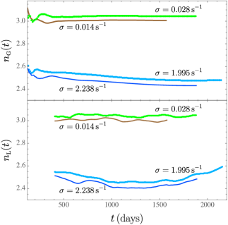
Figure 2: Global [upper panel, Eq. (17)] and local [lower panel, Eq. (18)] braking indices calculated from the simulation data for some representative values of the dissipation parameter $\sigma$. Note that there is no direct relationship between the magnitude of the dissipation process and the order of the braking indices when small variations of $\sigma$ are considered. However, on average, a more intense dissipation process (larger $\sigma$ values) leads to smaller values for the braking index.

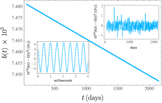
Figure 3: Time evolution of $b(t)$ as the pulsar slows down. The upper inset depicts the behavior of the normalized $b(t)$, obtained when its time-evolving equilibrium point $\Omega(t)^{2}/(3\gamma)$ is subtracted, thus showing that it is a highly oscillating function in time but on a small amplitude scale. The lower inset presents a close-up of the normalized curve (about day 2000) in a scale of milliseconds, showing that the oscillations occur with a well defined frequency, approximately the natural frequency $\sqrt{\gamma}/(2\pi)$ of the harmonic oscillator described by Eq. (12).

Following the model described in the previous section, the evolution of the system is governed by the coupled nonlinear differential equations given by Eqs. (16). The initial angular velocity is set to be $\Omega(0)=188.5\,{\rm rad}\cdot{\rm s}^{-1}$. The initial deformation of the body, $b(0)$, is assumed to be the equilibrium value of $b(t)$ in Eq. (16b), i.e., $b(0)=\Omega(0)^{2}/(3\gamma)\approx 7.482\times 10^{-5}$, for which $\dot{b}(0)$ was set to zero.

With the above assumptions, it follows that the underlying parameters are given by $\beta\approx 3.542\times 10^{-16}\,{\rm s}$ and $\gamma\approx 1.583\times 10^{8}\,{\rm s}^{-2}$. The remaining parameter $\sigma$ is associated to the dissipation processes during the oscillations of the quadrupole moment of the body, and will be adjusted in the simulations in order to obtain the braking index of the pulsar.

In a fashion similar to that present in the analysis in the existing literature for the calculation of the braking index of the Crab pulsar lyne2015 , we consider here the following method, that can be applied to both simulated or measured data:

1. Let $(t,\Omega)=(t_{k},\Omega_{k})$, for $k=1,\cdots,N$, denote the complete time series for the angular velocity of the pulsar;

2. For each $j$ such that $1<j\leq N$, the global braking index at time $t_{j}$ is computed by fitting the points $(t_{k},\Omega_{k})$, where $k=1,\cdots,j$, with the 3rd-degree polynomial

   $$P_{\textsc{g};j}(t)=\sum_{k=0}^{3}a_{k;j}\left(t-t_{\textsc{g};j}\right)^{k},$$

   where $t_{\textsc{g};j}=\frac{1}{2}\left(t_{j}-t_{0}\right)$ is the half time of the interval $[0,t_{j}]$, and the corresponding braking index at $t_{j}$ is given by Eq. (3), reading here

   $$n_{\textsc{g}}(t_{j})=\frac{\ddot{P}_{\textsc{g};j}(t_{\textsc{g};j})P_{\textsc{g};j}(t_{\textsc{g};j})}{\dot{P}_{\textsc{g};j}^{2}(t_{\textsc{g};j})}=2\frac{a_{2;j}a_{0;j}}{a_{1;j}^{2}};$$ (17)

3. The local braking index at time $t_{j}$ must be determined over each data subset with a fixed size $\Delta N\in\mathbb{N}$ as illustrated below:

   In this case, for each $\Delta N<j\leq N$, the local braking index at time $t_{j}>t_{\Delta N}$ is computed by fitting the points $(t_{k},\Omega_{k})$, where $k=j-\Delta N,\cdots,j$, with the 3rd-degree polynomial

   $$P_{\textsc{l};j}(t)=\sum_{k=0}^{3}a_{k;j}\left(t-t_{\textsc{l};j}\right)^{k},$$

   where $t_{\textsc{l};j}=\frac{1}{2}\left(t_{j-\Delta N}+t_{j}\right)$ is the center of the interval $[t_{j-\Delta N},t_{j}]$, and the corresponding local braking index is again given by Eq. (3), namely

   $$n_{\textsc{l}}(t_{j})=\frac{\ddot{P}_{\textsc{l};j}(t_{\textsc{l};j})P_{\textsc{l};j}(t_{\textsc{l};j})}{\dot{P}_{\textsc{l};j}^{2}(t_{\textsc{l};j})}=2\frac{b_{2;j}b_{0;j}}{b_{1;j}^{2}}.$$ (18)

An extrapolation-algorithm, based on the explicit midpoint rule, with stepsize control and order selection (see Section II.9 from Ref. Hairer1993 ) was used to numerically integrate the coupled system described by Eqs. (16a) and (16b), leading to the results depicted in Figs. 2 to 3. The integration spans a time window of about 5 years, which was enough to obtain solutions with stable braking indices. In fact, after a short time of instability, $n(t)$ eventually behaves as a slowly evolving function of time, as it can be confirmed by direct inspection of Fig. 2, where some solutions presenting positive braking indices were selected.

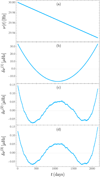
Figure 4: Rotational frequency (a) and residuals of the first (b), second (c) and third-order (d) shown as functions of time (in days) for the simulation data corresponding to a dissipation parameter $\sigma=1.995\,\mbox{s}^{-1}$. The global braking index corresponding to this simulation data, after about 6 years of integration time, achieves a value of approximately 2.5, as can be inferred by direct inspection of Fig. 2. The initial frequency in this simulation was $30.00\mbox{Hz}$.

The magnitude of the dissipation process associated with the quadrupole oscillations is dominant in determining the behavior of the braking index of the system. Processes for which $\sigma$ is of the order of $0.01\,\mbox{Hz}$ lead to braking indices around $n=3$, which is the expected result when the pulsar’s rotational energy is taken away only by means of magnetic dipole radiation. However, for higher values of $\sigma$, richer scenarios appear, as shown in Fig. 2. In particular, when $\sigma\approx 2\,\mbox{Hz}$, the solutions exhibit braking indices around 2.5. Small variations of $\sigma$ lead to different solutions for $n(t)$. On the other hand, this function does not seem to be very sensitive to small variations of the other parameters. The local behavior of the braking index, depicted in the lower panel of Fig. 2, was obtained using a moving average ($\Delta N$) of 400 days, which explains why it starts after the global index (upper panel). When a sufficiently high dissipation process is taken into account, the simulations suggest that even negative braking indices are possible solutions. This is an aspect that deserves further examination.

The behavior of the angular velocity is very similar for all solutions examined in Fig. 2. If the curves corresponding to the angular velocities for these models were included in a same plot, almost no visual difference would be seen. In fact, it can be shown that for any instant of time in the simulations, the difference between the angular velocities of any of these solutions is smaller than $10^{-5}\mbox{Hz}$.

The behavior of $b(t)$ for the model with $\sigma=1.995\,\mbox{s}^{-1}$ is shown in Fig. 3. In the plot scale it looks like a slowly decreasing monotonic function of time. However, a more detailed examination shows that $b(t)$ is a highly oscillatory function around the time-dependent equilibrium point $\Omega(t)^{2}/(3\gamma)$, as highlighted in the inserts. Indeed, due to their mutual coupling, both $b(t)$ and $\Omega(t)$ decompose into a slow monotonically decreasing component and a fast (and tiny) oscillatory component; the slow component can be extracted out by calculating the difference $b(t)-\Omega(t)^{2}/(3\gamma)$. Thus, as the system loses energy by means of MDR emission and oscillation damping, it will slow-down its rotation frequency and also the amplitude of the oscillations.

The evolution of the rotation frequency corresponding to the model with $\sigma=1.995\,\mbox{s}^{-1}$ is depicted in Fig. 4(a), which is a solution presenting a braking index of approximately $2.5$. The other panels in the figure show the residuals of the first, second and third order, which were obtained following the standard procedure (see for instance the analysis for the Crab pulsar lyne2015 ): the data set is fitted by means of a $k$-degree polynomial, which can be written as $\nu(t)=\sum_{i=0}^{k}c_{i}(t-t_{0})^{i}+\delta\nu^{(k)}$, where $t_{0}$ is chosen, for instance, to be the medium time of the data set, the coefficients $c_{i}$ are obtained by the fitting procedure, and the time-dependent function $\delta\nu^{(k)}$ is the $k$-th order residual obtained when the $k$-th order fitting polynomial is subtracted from the data. For instance, Fig. 4(b) depicts the first-order residual $\delta\nu^{(1)}=[\nu(t)]_{\mbox{\tiny data}}-[c_{0}+c_{1}(t-t_{0})]$, where $t_{0}=9.299\times 10^{7}\,\mbox{s}\approx 1076\,\mbox{days}$, $c_{0}\approx 29.97\,\mbox{Hz}$, and $c_{1}\approx-3.757\times 10^{-10}\,\mbox{s}^{-2}$.

The residuals at second and third order exhibit some irregularities, which cannot be attributed to numerical errors. They can be interpreted as very short moments in time during which the angular momentum is suddenly changed before the star returns to its original state. That could be interpreted as micro-glitches: a realistic model would describe for instance various rotating shells, all of which would be subject to equations similar to those presented here and somehow interacting. Could such a more elaborate model enhance this phenomenon to the level of the observed glitches?

IV A note about glitches: the behavior of the Crab pulsar

Having described our simple model, one wants to compare with the existing data relevant to the dynamical range under investigation. The best example one can think of is provided by the enormous amount of data available concerning the Crab pulsar.

The Crab pulsar (PSR B0531+21) is an isolated neutron star whose angular velocity deceleration has been measured since the 1970s. Monthly spaced pulsar timing measurements have been taken by Jodrell Bank Observatory since 1982 lyne1993 . In Fig. 5(a), the rotation frequency measured for the Crab pulsar is shown as a function of time, from MJD 45015 (February 15, 1982) to MJD 59806 (August 15, 2022) lyne1993 . The residuals are shown from top to bottom [panels (b) to (d)], where the coefficients of the third-order polynomial fitting are $t_{0}=6.389712\times 10^{8}\,\mbox{s}=7395.5\,\mbox{days}$, $c_{0}\approx 31.36\,\mbox{Hz}$, $c_{1}\approx-4.205\times 10^{-10}\,\mbox{s}^{-2}$, $c_{2}\approx 6.728\times 10^{-21}\,\mbox{s}^{-3}$, and $c_{3}\approx-1.260\times 10^{-31}\,\mbox{s}^{-4}$.

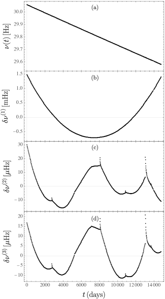
Figure 5: Rotation frequency and residuals of the Crab pulsar, according to data collected from 1982 onwards lyne1993 ; lyne2015 . The starting time in this figure corresponds the MJD 45015, for which the measured frequency was $\nu=30.0592241133\,\mbox{Hz}$. The residuals of second and third orders, depicted in panels (c) and (d), respectively, clearly show a rich glitch activity of the pulsar in this period.

This system has occasional glitches, in which the star is spinned-up for a short period of time and returns to its former rotation frequency within an interval of about 20 days. The glitch activities can be clearly seen in Fig. 5(c) and 5(d). They contribute massively to the global braking index. The global and local indices agree with the constant value $n\approx 2.5$ if and only if they are computed in an interval not containing a glitch. However, the global braking index decreases monotonically in time as multiple intervals are included in the data set so that its final value reaches $n\approx 2.3$ lyne2015 .

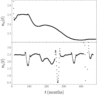
Figure 6: Braking index as function of time for the Crab pulsar. Here the index is calculated using the global and local procedures discussed in the last section, as depicted in upper and lower panels, respectively. A moving average with $\Delta N=30$ was here used to obtain the local index.

Global and local behaviors of the braking index with time are shown in Fig. 6, upper and lower panels respectively. In particular, the local index as a function of time (in months) is shown in lower panel of Fig. 6, where the moving average was calculated using a window containing 30 successive measurements. It can be seen that after each glitch, the braking index returns approximately to the value it had before the glitch, and this happens in less than a month. However, its influence in the local braking index calculation goes way longer, an aspect that is dependent on the choice of $\Delta N$.

V Final remarks

In this work, we explored the idea that as MDR is emitted by an isolated pulsar, its energy is continuously driven away, causing a slow-down of its spin, and a possible modification of the shape of the star. Although the MDR emission is largely accepted in the literature, adding a perturbation in its ellipsoidal shape by means of small oscillations has never been considered. As the star cannot be strictly rigid, oscillations are expected: they are produced almost in a stationary regime as it is linked to the spin slow-down process. These oscillations must be dissipated by internal phenomena leading to a secondary form of energy loss by the star. The possible mechanisms behind such dissipation of energy were not considered in details in this work. Instead, it was assumed that the effect is described by an effective damping process that is dependent of the velocity square of the quadrupole moment oscillations, leanding to a forced (by means of MDR emission) and damped linear differential equation governing the evolution of the body oscillations. In planetary tide theory terminology, this equation describes a Kelvin-Voigt damping of the quadrupole moment oscillations, endowed with a deformation inertia term Lucas2018 . Additionally, the equation of motion for the angular momentum of the star generalizes previous treatments where the contribution due to the time-dependent moment of inertia was ignored. As a consequence of this description, solutions presenting braking indices below the predicted value for a pure MDR model ($n_{\textsc{mdr}}=3$) were found by means of numerical calculations. In particular, we found that there exist choices for the phenomenological parameters for which the solutions exhibit values similar to those measured in isolated pulsars.

It should be noticed that the braking index calculated by means of the global method is highly dependent on the initial conditions of the system. Furthermore, if glitches occur during the evolution, as is the case in most of the isolated pulsars, they can significantly contribute to the value of this index. This aspect can be appreciated, for instance, in the case of the Crab pulsar lyne2015 , where the value of $n$ calculated by means of the local method results in $n_{\textsc{l}}=2.51$, while the global method leads to $n_{\textsc{g}}=2.34$. If the data set is restricted to the period from 1982 onwards, the global method would result in a different value, while the local index would not be significantly affected, as discussed in the previous section. This suggests that the local method provides a more robust index to describe the slow-down of isolated pulsars.

The exact reason behind the occurrence of glitches in an isolated pulsar is still a matter of investigation. Most likely, they are associated with redistribution of mass in short time intervals activated by resonance phenomena throughout the evolution of the system. After a glitch, the system approximately returns smoothly to its former state. In the idealized model we investigated here, it is assumed that the shape of the star evolves in time, as governed by the oscillating function $b(t)$. Thus, after the initial transient, the ellipsoid describing the star’s surface will oscillate with an almost constant amplitude. In this scenario, localized sub-micro glitches are expected to occur all the time, as suggested by the zigzags in the second and third-order residuals appearing in Fig. 4. A more elaborate model could shed more light on this important issue. Consider a multi-layer model for instance. In such a model, resonance effects between the different layer oscillations could lead to significant mass redistribution, and possibly to macroscopic glitches, that would then have to be compare to those observed in isolated pulsars. This is an issue that deserves investigation.

Among the possible applications of this work, it should be mentioned that the experimental knowledge of the rotation frequency curve of a given pulsar could be used as a starting point to find the best set of physical parameters behind its behavior. It should be noted however that the damping effects over the oscillations due to emission of thermal radiation and quadrupole gravitational radiation for instance, are not yet fully understood for such systems and also deserve further investigation. Models assuming different forms for the dissipation function and its implications in the possible values of $n$ could be of great value in such investigations.

- (1) A. Hewish, S. J. Bell, J. D. H. Pilkington, P. F. Scott, and R. A. Collins, Observation of a rapidly pulsating radio source, Nature 217, 709 (1968).
- (2) T. Gold, Rotating neutron stars as the origin of the pulsating radio sources, Nature 218, 731 (1968).
- (3) Richards, D., IAU Astronomical Telegram Circular No. 2114 (1968).
- (4) F. Pacini, Energy emission from a neutron star, Nature 216, 567 (1967).
- (5) F. Pacini, Rotating neutron stars, pulsars and supernova remnants, Nature 219, 145 (1968).
- (6) J. E. Gunn and J. P. Ostriker, Magnetic dipole radiation from pulsars, Nature 221, 454 (1969).
- (7) S. A. Teukolsky, S. L. Shapiro, Black holes, white dwarfs, and neutron stars (Wiley-VCH, Weinheim, 2004), Sec. 10.5.
- (8) H. C. Goldwire Jr., and F. C. Michel, Analysis of the slowing-down rate of NP 0532, Ap. J. 156, L111 (1969).
- (9) J. E. Gunn and J. P. Ostriker, On the nature of pulsars. I. theory, Ap. J. 157, 1395 (1969).
- (10) A. G. Lyne, C. A. Jordan, F. Graham-Smith, C. M. Espinoza, B. W. Stappers, and P. Weltevrede, 45 years of rotation of the Crab pulsar, MNRAS 446, 857 (2015).
- (11) R. D. Blandford and R. W. Romani, On the interpretation of pulsar braking indices, MNRAS 234, 57P (1988).
- (12) N. S. Magalhães, T. A. Miranda, and C. Frajuca, Predicting ranges for pulsars’ braking indices, Ap. J. 755, 54 (2012).
- (13) O. Hamil, J. R. Stone, M. Urbanec, and G. Urbancová, Braking index of isolated pulsars, Phys. Rev. D 91, 063007 (2015).
- (14) O. Hamil, N. J. Stone, and J. R. Stone, Braking index of isolated pulsars. II. A novel two-dipole model of pulsar magnetism, Phys. Rev. D 94, 063012 (2016).
- (15) C. Ragazzo and L. S. Ruiz, Dynamics of an isolated, viscoelastic, self-gravitating body, Celest. Mech. Dyn. Astr. 122, 303 (2015).
- (16) J. Baillieul and M. Levi, Rotational elastic dynamics, Physica D: Nonlinear Phenomena 27(1-2), 43-62 (1987).
- (17) C. Ragazzo and L. S. Ruiz, Viscoelastic tides: models for use in Celestial Mechanics, Celest. Mech. Dyn. Astr. 128, 19-59 (2017).
- (18) E. Hairer, S. P. Norsett and G. Wanner, Solving ordinary differential equations I: Nonstiff Problems, Springer Berlin Heidelberg, (1993).
- (19) A. G. Lyne, R. S. Pritchard, and F. Graham-Smith, 23 years of Crab pulsar rotational history, MNRAS, 265, 1003 (1993) http://www.jb.man.ac.uk/ pulsar/crab.html.
- (20) A. C. M. Correia, C. Ragazzo and L. S. Ruiz, The effects of deformation inertia (kinetic energy) in the orbital and spin evolution of close-in bodies, Celest. Mech. Dyn. Astr. 130, 1-30 (2018).