Abstract

Measurement error is ubiquitous in many variables – from blood pressure recordings in physiology to intelligence measures in psychology. Structural equation models (SEMs) account for the process of measurement by explicitly distinguishing between latent variables and their measurement indicators. Users often fit entire SEMs to data, but this can fail if some model parameters are not identified. The model-implied instrumental variables (MIIVs) approach is a more flexible alternative that can estimate subsets of model parameters in identified equations. Numerous methods to identify individual parameters also exist in the field of graphical models (such as DAGs), but many of these do not account for measurement effects. Here, we take the concept of “latent-to-observed” (L2O) transformation from the MIIV approach and develop an equivalent graphical L2O transformation that allows applying existing graphical criteria to latent parameters in SEMs. We combine L2O transformation with graphical instrumental variable criteria to obtain an efficient algorithm for non-iterative parameter identification in SEMs with latent variables. We prove that this graphical L2O transformation with the instrumental set criterion is equivalent to the state-of-the-art MIIV approach for SEMs, and show that it can lead to novel identification strategies when combined with other graphical criteria.

1 INTRODUCTION

Graphical models such as directed acyclic graphs (DAGs) are currently used in many disciplines for causal inference from observational studies. However, the variables on the causal pathways modelled are often different from those being measured. Imperfect measures cover a broad range of sciences, including health and medicine (e.g., blood pressure, oxygen level), environmental sciences (e.g., measures of pollution exposure of individuals), and the social (e.g., measures of socioeconomic status) and behavioral sciences (e.g., substance abuse).

Many DAG models do not differentiate between the variables on the causal pathways and their actual measurements in a dataset (Tennant et al.,, 2019). While this omission is defensible when the causal variables can be measured reliably (e.g., age), it becomes problematic when the link between a variable and its measurement is more complex. For example, graphical models employed in fields like Psychology or Education Research often take the form of latent variable structural equation models (LVSEMs, Figure 1; Bollen, (1989)), which combine a latent level of unobserved variables and their hypothesized causal links with a measurement level of their observed indicators (e.g., responses to questionnaire items). This structure is so common that LVSEMs are sometimes simply referred to as SEMs. In contrast, models that do not differentiate between causal factors and their measurements are traditionally called simultaneous equations or path models.

Once a model has been specified, estimation can be performed in different ways. SEM parameters are often estimated all at once by iteratively minimizing some difference measure between the observed and the model-implied covariance matrices. However, this “global” approach has some pitfalls. First, all model parameters must be algebraically identifiable for a unique minimum to exist; if only a single model parameter is not identifiable, the entire fitting procedure may not converge (Boomsma,, 1985) or provide meaningless results. Second, local model specification errors can propagate through the entire model (Bollen et al.,, 2007). Alternatively, Bollen, (1996) introduced a “local”, equation-wise approach for SEM parameter identification termed “model-implied instrumental variables” (MIIVs), which is non-iterative and applicable even to models where not all parameters are simultaneously identifiable. MIIV-based SEM identification is a mature approach with a well-developed underlying theory as well as implementations in multiple languages, including R (Fisher et al.,, 2019).

Figure 1: SEM based on the Industrialization and Political Democracy model (Bollen,, 1989) with latent variables $l_{1}$ (industrialization), and $l_{2}$ (political democracy). The model contains 3 indicators for $l_{1}$: (1) gross national product ($y_{1}$), (2) energy consumption ($y_{2}$), and (3) labor force in industry ($y_{3}$), and 4 indicators for $l_{2}$: (1) press freedom rating ($y_{4}$), (2) political opposition freedom ($y_{5}$), (3) election fairness ($y_{6}$), and (3) legislature effectiveness ($y_{7}$). $\lambda_{11}\dots\lambda_{13},\lambda_{24}\dots\lambda_{27},\text{ and }\beta_{11}$ are the path coefficients. $\epsilon_{1},\dots,\epsilon_{7},\text{ and }\zeta_{1}$ represent noise/errors.

Of all the model parameters that are identifiable in principle, any given estimator (such as the MIIV-based approach) can typically only identify parameters in identified equations and identified parameters in underidentified equations. Different identification methods are therefore complementary and can allow more model parameters to be estimated. Having a choice of such methods can help users to keep the stages of specification and estimation separated. For example, a researcher who only has access to global identification methodology might be tempted to impose model restrictions just to “get a model identified” and not because there is a theoretical rationale for the restrictions imposed. With more complementary methods to choose from, researchers can instead base model specification on substantive theory and causal assumptions.

The development of parameter identification methodology has received intense attention in the graphical modeling field. The most general identification algorithm is Pearl’s do-calculus, which provides a complete solution in non-parametric models (Huang and Valtorta,, 2006; Shpitser and Pearl,, 2006). The back-door and front-door criteria provide more convenient solutions in special cases (Pearl,, 2009). While there is no practical general algorithm to decide identifiability for models that are linear in their parameters, there has been a flurry of work on graphical criteria for this case, such as instrumental sets (Brito and Pearl,, 2002), the half-trek criterion (Foygel et al.,, 2012), and auxiliary variables (Chen et al.,, 2017). Unfortunately, these methods were all developed for the acyclic directed mixed graph (ADMG) framework and require at least the variables connected to the target parameter to be observed – which is rarely the case in SEMs. Likewise, many criteria in graphical models are based on “separating” certain paths by conditioning on variables, whereas no such conditioning-based criteria exist for SEMs.

The present paper aims to make identification methods from the graphical model literature available to the SEM field. We offer the following contributions:

• We note that Bollen, (1996)’s latent-to-observed (L2O) transformation that transforms a latent variable SEM into a model with only observed variables can be used more generally in models containing arbitrary mixtures of latent and observed variables (Section 3).

• We present a graphical equivalent of L2O transformation that allows us to apply known graphical criteria to SEMs (Section 4).

• We prove that Bollen’s MIIV approach (Bollen,, 1996; Bollen and Bauer,, 2004; Bollen et al.,, 2022) is equivalent to a graphical L2O transformation followed by the application of the graphical instrumental set criterion (Brito and Pearl, (2002); Section 5).

• We give examples where the graphical L2O transformation approach can identify more parameters compared to the MIIV approach implemented in the R package MIIVsem (Fisher et al., (2019); Section 6).

Thus, by combining the L2O transformation idea from the SEM literature with identification criteria from the graphical models field, we bridge these two fields – hopefully to the benefit of both.

2 BACKGROUND

In this section, we give a brief background on basic graphical terminology and define SEMs.

2.1 Basic Terminology

We denote variables using lowercase letters ($x_{i}$), sets and vectors of variables using uppercase letters ($X$), and matrices using boldface ($\bm{\Lambda}$). We write the cardinality of a set $V$ as $|V|$, and the rank of a matrix $\bm{\Lambda}$ as $\textrm{rk}(\bm{\Lambda})$. A mixed graph (or simply graph) ${\cal G}=(V,A)$ is defined by sets of variables (nodes) $V=\{x_{1},\ldots,x_{n}\}$ and arrows $A$, where arrows can be directed ($x_{i}\to x_{j}$) or bi-directed $(x_{i}\leftrightarrow x_{j})$. A variable $x_{i}$ is called a parent of another variable $x_{j}$ if $x_{i}\to x_{j}\in A$, or a spouse of $x_{j}$ if $x_{i}\leftrightarrow x_{j}\in A$. We denote the set of parents of $x_{i}$ in ${\cal G}$ as $Pa_{\cal G}(x_{i})$.

Paths: A path of length $k$ is a sequence of $k$ variables such that each variable is connected to its neighbours by an arrow. A directed path from $x_{i}$ to $x_{j}$ is a path on which all arrows point away from the start node $x_{i}$. For a path $\pi$, let $\pi[x_{i}\sim x_{j}]$ denote its subsequence from $x_{i}$ to $x_{j}$, in reverse order when $x_{i}$ occurs after $x_{j}$; for example, if $\pi=x_{1}\leftarrow x_{2}\to x_{3}$ then $\pi[x_{2}\sim x_{3}]=x_{2}\to x_{3}$ and $\pi[x_{1}\sim x_{2}]=x_{2}\to x_{1}$. Importantly, this definition of a path is common in DAG literature but is different from the SEM literature, where “path” typically refers to a single arrow between two variables. Hence, a path in a DAG is equivalent to a sequence of paths in path models. An acyclic directed mixed graph (ADMG) is a mixed graph with no directed path of length $\geq 2$ from a node to itself.

Treks and Trek Sides: A trek (also called open path) is a path that does not contain a collider, that is, a subsequence $x_{i}\to x_{j}\leftarrow x_{k}$. A path that is not open is a closed path. Let $\pi$ be a trek from $x_{i}$ to $x_{j}$, then $\pi$ contains a unique variable $t$ called the top, also written as $\pi^{\leftrightarrow}$, such that $\pi[t\sim x_{i}]$ and $\pi[t\sim x_{j}]$ are both directed paths (which could both consist of a single node). Then we call $\pi^{\leftarrow}:=\pi[t\sim x_{i}]$ the left side and $\pi^{\to}:=\pi[t\sim x_{j}]$ the right side of $\pi$.

Trek Intersection: Consider two treks $\pi_{i}$ and $\pi_{j}$, then we say that $\pi_{i}$ and $\pi_{j}$ intersect if they contain a common variable $v$. We say that they intersect on the same side (have a same-sided intersection) if $v$ occurs on $\pi_{i}^{\leftarrow}$ and $\pi_{j}^{\leftarrow}$ or $\pi_{i}^{\to}$ and $\pi_{j}^{\to}$; in particular, if $v$ is the top of $\pi_{i}$ or $\pi_{j}$, then the intersection is always same sided. Otherwise, $\pi_{i}$ and $\pi_{j}$ intersect on opposite sides (have an opposite-sided intersection).

t-separation: Consider two sets of variables, $L$ and $R$, and a set $T$ of treks. Then we say that the tuple $(L,R)$ $t$-separates (is a $t$-separator of) $T$ if every trek in $T$ contains either a variable in $L$ on its left side or a variable in $R$ on the right side. For two sets of variables, $A$ and $B$, we say that $(L,R)$ $t$-separates $A$ and $B$ if it $t$-separates all treks between $A$ and $B$. The size of a $t$-separator $(L,R)$ is $|L|+|R|$.

2.2 Structural Equation Models

We now define structural equation models (SEMs) as they are usually considered in the DAG literature (e.g., Sullivant et al.,, 2010). This definition is the same as the Reticular Action Model (RAM) representation (McArdle and McDonald,, 1984) from the SEM literature. A structural equation model (SEM) is a system of equations linear in their parameters such that:

$$X=\bm{B}X+E$$

where $X$ is a vector of variables (both latent and observed), $\bm{B}$ is a $|X|\times|X|$ matrix of path coefficients, and $E=\{\epsilon_{1},\ldots,\epsilon_{|X|}\}$ is a vector of error terms with a positive definite covariance matrix $\bm{\Phi}$ (which has typically many or most of its off-diagonal elements set to 0) and zero means. The path diagram of an SEM $(\bm{B},\bm{\Phi})$ is a mixed graph with nodes $V=X\cup E$ and arrows $A=\{\epsilon_{i}\to x_{i}\mid i\in 1,\ldots,|X|\}\cup\{x_{i}\to x_{j}\mid\bm{B}[i,j]\neq 0\}\cup\{\epsilon_{i}\leftrightarrow\epsilon_{j}\mid i\neq j,\bm{\Phi}[i,j]\neq 0\}$. We also write $\beta_{x_{i}\to x_{j}}$ for the path coefficients in $\bm{B}$ and $\phi_{\epsilon_{i}}$ for the diagonal entries (variances) in $\bm{\Phi}$. Each equation in the model corresponds to one node in this graph, where the node is the dependent variable and its parent(s) are the explanatory variable(s). Each arrow represents one parameter to be estimated, i.e., a path coefficient (e.g., directed arrow between latents and observed variables), a residual covariance (bi-directed arrow), or a residual variance (directed arrow from error term to latent or indicator). However, some of these parameters could be fixed; for example, at least one parameter per latent variable needs to be fixed to set its scale, and covariances between observed exogenous variables (i.e., observed variables that have no parents) are typically fixed to their observed values. In this paper, we focus on estimating the path coefficients. We only consider recursive SEMs in this paper – i.e., where the path diagram is an ADMG – even though the methodology can be generalized.

Sullivant et al., (2010) established an important connection between treks and the ranks of submatrices of the covariance matrix, which we will heavily rely on in our paper.

Theorem 1.

Trek separation; (Sullivant et al.,, 2010, Theorem 2.8) Given an SEM $\cal G$ with an implied covariance matrix $\bm{\Sigma}$, and two subsets of variables $A,B\subseteq X$,

$$\text{rk}(\bm{\Sigma}[A,B])\leq\text{min}\left\{|L|+|R|\mid(L,R)\text{ t-separates }A\text{ and }B\right\}$$

where the inequality is tight for generic covariance matrices implied by $\cal G$.

In the special case $A=\{x_{1}\},B=\{x_{2}\}$, Theorem 1 implies that $x_{1}$ and $x_{2}$ can only be correlated if they are connected by a trek. Although the compatible covariance matrices of SEMs can also be characterized in terms of $d$-separation (Chen and Pearl,, 2014), we use $t$-separation for our purpose because it does not require conditioning on variables, and it identifies more constraints on the covariance matrix implied by SEMs than d-separation (Sullivant et al.,, 2010).

3 LATENT-TO-OBSERVED TRANSFORMATIONS FOR SEMS

A problem with IV-based identification criteria is that they cannot be directly applied to latent variable parameters. The MIIV approach addresses this issue by applying the L2O transformation to these model equations, such that they only consist of observed variables. The L2O transformation in Bollen, (1996) is presented on the LISREL representation of SEMs (see Supplementary Material). In this section, we first briefly introduce “scaling indicators”, which are required for performing L2O transformations. We then use it to define the L2O transformation on the RAM notation (defined in Section 2.2) and show that with slight modification to the transformation, we can also use it to partially identify equations. We will, from here on, refer to this transformation as the “algebraic L2O transformation” to distinguish it from the purely graphical L2O transformation that we introduce later in Section 4.

3.1 Scaling Indicators

The L2O transformation (both algebraic and graphical) uses the fact that any SEM is only identifiable if the scale of each latent variable is fixed to an arbitrary value (e.g., 1), introducing new algebraic constraints. These constraints can be exploited to rearrange the model equations in such a way that latent variables can be eliminated.

The need for scale setting is well known in the SEM literature and arises from the following lemma (since we could not find a direct proof in the literature – perhaps due to its simplicity – we give one in the Appendix).

Lemma 1.

(Rescaling of latent variables). Let $x_{i}$ be a variable in an SEM $(\bm{B},\bm{\Phi})$. Consider another SEM $(\bm{B}^{\prime},\bm{\Phi}^{\prime})$ where we choose a scaling factor $\alpha\neq 0$ and change the coefficients as follows: For every parent $p$ of $x_{i}$, $\beta_{p\to x_{i}}^{\prime}=\alpha^{-1}\;\beta_{p\to x_{i}}$; for every child $c$ of $x_{i}$, $\beta_{x_{i}\to c}^{\prime}=\alpha\;\beta_{x_{i}\to c}$; for every spouse $s$ of $x_{i}$, $\phi_{x_{i}\leftrightarrow s}^{\prime}=\alpha^{-1}\phi_{x_{i}\leftrightarrow s}$; and $\phi_{x_{i}}^{\prime}=\alpha^{-2}\phi_{x_{i}}$. Then for all $j,k\neq i$, $\bm{\Sigma}[j,k]=\bm{\Sigma}^{\prime}[j,k]$.

If $x_{i}$ is a latent variable in an SEM, then Lemma 1 implies that we will get the same implied covariance matrix among the observed variables for all possible scaling factors. In other words, we need to set the scale of $x_{i}$ to an arbitrary value to identify any parameters in such a model. Common choices are to either fix the error variance of every latent variable such that its total variance is $1$, or to choose one indicator per latent and set its path coefficient to $1$. The latter method is often preferred because it is simpler to implement. The chosen indicators for each latent are then called the scaling indicators. However, note that Lemma 1 tells us that we can convert any fit based on scaling indicators to a fit based on unit latent variance, so this choice does not restrict us in any way.

3.2 Algebraic L2O Transformation for RAM

The main idea behind algebraic L2O transformation is to replace each of the latent variables in the model equations by an observed expression involving the scaling indicator. As in Bollen, (1996), we assume that each of the latent variables in the model has a unique scaling indicator. We show the transformation on a single model equation to simplify the notation. Given an SEM $\cal G$ on variables $X$, we can write the equation of any variable $x_{i}\in X$ as:

$$x_{i}=\epsilon_{i}+\sum_{x_{j}\in Co(x_{i})}\beta_{x_{j}\rightarrow x_{i}}x_{j}$$

where $Co(x_{i})=\{Co_{l}(x_{i}),Co_{o}(x_{i})\}$ is the set of covariates in the equation for $x_{i}$. $Co_{l}(x_{i})$ and $Co_{o}(x_{i})$ are the latent and observed covariates, respectively. Since each latent variable $x_{j}$ has a unique scaling indicator $x_{j}^{s}$, we can write the latent variable as $x_{j}=x_{j}^{s}-\epsilon_{x_{j}^{s}}$. Replacing all the latents in the above equation with their scaling indicators, we obtain:

$$x_{i}=\epsilon_{i}+\sum_{x_{j}\in Co_{l}(x_{i})}\beta_{x_{j}\rightarrow x_{i}}(x_{j}^{s}-\epsilon_{x_{j}^{s}})+\sum_{x_{k}\in Co_{o}(x_{i})}\beta_{x_{k}\rightarrow x_{i}}x_{k}$$

If $x_{i}$ is an observed variable, the transformation is complete as the equation only contains observed variables. But if $x_{i}$ is a latent variable, we can further replace $x_{i}$ as follows:

$$x_{i}^{s}=\epsilon_{i}+\epsilon_{x_{i}^{s}}+\sum_{x_{j}\in Co_{l}(x_{i})}\beta_{x_{j}\rightarrow x_{i}}(x_{j}^{s}-\epsilon_{x_{j}^{s}})+\sum_{x_{k}\in Co_{o}(x_{i})}\beta_{x_{k}\rightarrow x_{i}}x_{k}$$

As the transformed equation now only consists of observed variables, IV-based criteria can be applied to check for identifiability of parameters.

3.3 Algebraic L2O Transformations for Partial Equation Identification

In the previous section, we used the L2O transformation to replace all the latent variables in the equation with their scaling indicators, resulting in an equation with only observed variables. An IV-based estimator applied to these equations would try to estimate all the parameters together. However, there are cases (as shown in Section 6) where not all of the parameters of an equation are identifiable. If we apply L2O transformation to the whole equation, none of the parameters can be estimated.

Here, we outline an alternative, “partial” L2O transformation that replaces only some of the latent variables in the equation. Assuming $Co_{l}^{i}(x_{i})\subset Co_{l}(x_{i})$ as the set of latent variables whose parameters we are interested in estimating, we can write the partial L2O transformation as:

$$\begin{split}x_{i}=\epsilon_{i}+&\sum_{x_{j}\in Co_{l}^{i}(x_{i})}\beta_{x_{j}\rightarrow x_{i}}(x_{j}^{s}-\epsilon_{x_{j}^{s}})+\\ &\sum_{x_{k}\in Co_{l}(x_{i})\setminus Co_{l}^{i}(x_{i})}\beta_{x_{k}\rightarrow x_{i}}x_{k}+\sum_{x_{l}\in Co_{o}(x_{i})}\beta_{x_{l}\rightarrow x_{i}}x_{l}\end{split}$$

Similar to the previous section, we can further apply L2O transformation for $x_{i}$ if it is also a latent variable. As the parameters of interest are now with observed covariates in the transformed equation, IV-based criteria can be applied to check for their identifiability while treating the variables in $Co_{l}(x_{i})\setminus Co_{l}^{i}(x_{i})$ as part of the error term.

4 GRAPHICAL L2O TRANSFORMATION

Having shown the algebraic L2O transformation, we now show that these transformations can also be done graphically for path diagrams. An important difference is that the algebraic transformation is applied to all equations in a model simultaneously by replacing all latent variables, whereas we apply the graphical transform only to a single equation at a time (i.e., starting from the original graph for every equation). Applying the graphical transformation to multiple equations simultaneously results in a non-equivalent model with a different implied covariance matrix.

Given an SEM $\cal G$, the equation for any variable $x_{j}$ can be written in terms of its parents in the path diagram as: $x_{j}=\sum_{x_{k}\in\textrm{Pa}_{\cal G}(x_{j})}\beta_{x_{k}\to x_{j}}x_{k}+\epsilon_{x_{j}}$. Using this equation, we can write the relationship between any latent variable $x_{j}$ and its scaling indicator $x_{j}^{s}$ as (where $\beta_{x_{j}\to x_{j}^{s}}$ is fixed to $1$):

$$x_{j}=x_{j}^{s}-\epsilon_{x_{j}^{s}}-\sum_{x_{k}\in\textrm{Pa}_{\cal G}(x_{j}^{s})\setminus x_{j}}\beta_{x_{k}\to x_{j}^{s}}x_{k}$$ (1)

We use this graphical L2O transformation as follows. Our goal is to identify a path coefficient $\beta_{x_{i}\to x_{j}}$ in a model $\cal G$. If both $x_{i}$ and $x_{j}$ are observed, we leave the equation untransformed and apply graphical identification criteria (Chen and Pearl,, 2014). Otherwise, we apply the graphical L2O transformation to $\cal G$ with respect to $x_{i}$, $x_{j}$, or both variables – ensuring that the resulting model ${\cal G}^{\prime}$ contains an arrow between two observed variables $x_{i}^{\prime}$ and $x_{j}^{\prime}$, where the path coefficient $\beta_{x_{i}^{\prime}\to x_{j}^{\prime}}$ in ${\cal G}^{\prime}$ equals $\beta_{x_{i}\to x_{j}}$ in $\cal G$.

We now illustrate this approach on an example for each of the three possible combinations of latent and observed variables.

(a)

(b)

(c)

Figure 2: Example L2O transformations for path coefficients (a) from a latent to an observed variable; (b) from an observed to a latent variable; (c) between two latent variables.

Latent-to-observed arrow: Consider the arrow $l_{1}\to y_{3}$ in Figure 2(a), and let $\beta$ be the path coefficient of this arrow. To perform the L2O transformation, we start with the model equation involving $\beta$:

$$y_{3}=\beta l_{1}+\beta_{y_{5}\to y_{3}}y_{5}+\epsilon_{3}$$

We then use Equation 1 to write the latent variable, $l_{1}$ in terms of its scaling indicator, $y_{2}$ as: $l_{1}=y_{2}-\epsilon_{2}+\beta_{y_{1}\to y_{2}}y_{1}$, and replace it in the above equation to obtain:

$$y_{3}=\beta y_{2}-\beta\beta_{y_{1}\to y_{2}}y_{1}+\beta_{y_{5}\to y_{3}}y_{5}-\beta\epsilon_{2}+\epsilon_{3}$$

The transformation has changed the equation for $y_{3}$, which now regresses on the observed variables $y_{2}$, $y_{1}$, and $y_{5}$, as well as the errors $\epsilon_{2}$ and $\epsilon_{3}$. We make the same changes in the graphical structure by adding the arrows $y_{2}\to y_{3}$, $y_{1}\to y_{3}$, $\epsilon_{2}\to y_{3}$, and removing the arrow $l_{1}\to y_{3}$.

Observed-to-latent arrow: Consider the arrow $y_{1}\to l_{1}$ in Figure 2(b) with coefficient $\beta$. For L2O transformation in this case, we apply Equation 1 to replace $l_{1}$ in the model equation $l_{1}=\beta y_{1}+\zeta_{1}$ to obtain:

$$y_{4}=\beta y_{1}+\beta_{y_{3}\to y_{4}}y_{3}+\beta_{y_{2}\to y_{4}}y_{2}+\zeta_{1}+\epsilon_{4}$$

The equivalent transformation to the path diagram consists of adding the arrows $y_{1}\to y_{4}$, and $\zeta_{1}\to y_{4}$, and removing the arrows: $l_{1}\to y_{4}$ and $y_{1}\to l_{1}$.

Latent-to-latent arrow: Consider the arrow $l_{1}\to l_{2}$ in Figure 2(c) with coefficient $\beta$. In this case, we again apply Equation 1 to replace both $l_{1}$ and $l_{2}$ in the model equation for $l_{2}=\beta l_{1}+\zeta_{2}$. This is equivalent to applying two L2O transformations in sequence and leads to the transformed equation:

$$y_{2}=\beta y_{1}-\beta\epsilon_{1}+\zeta_{2}+\epsilon_{2}$$

Equivalently, we now add the arrows $y_{1}\to y_{2}$, $\zeta_{2}\to y_{2}$, and $\epsilon_{1}\to y_{2}$. We also remove the arrows $l_{2}\to y_{2}$ and $l_{1}\to l_{2}$.

5 MODEL-IMPLIED INSTRUMENTAL VARIABLES ARE EQUIVALENT TO INSTRUMENTAL SETS

After applying the L2O transformations from the previous sections, we can use either algebraic or graphical criteria to check whether the path coefficients are identifiable. In this section, we introduce the Instrumental set criterion (Brito and Pearl,, 2002) and the MIIV approach from Bollen, (1996) that precedes it, and show that they are equivalent. Importantly, even though we refer to the MIIV approach as an algebraic criterion to distinguish it from the graphical criterion, it is not a purely algebraic approach and utilizes the graphical structure of the model to infer correlations with error terms.

We will first focus on the instrumental set criterion proposed by Brito and Pearl, (2002). We state the criterion below in a slightly rephrased form that is consistent with our notation in Section 2:

Definition 1 (Instrumental Sets (Brito and Pearl,, 2002)).

Given an ADMG $\cal G$, a variable $y$, and a subset $X$ of the parents of $y$, a set of variables $I$ fulfills the instrumental set condition if for some permutation $i_{1}\ldots i_{k}$ of $I$ and some permutation $x_{1}\ldots x_{k}$ of $X$ we have:

1. There are no treks from $I$ to $y$ in the graph ${\cal G}_{\overline{X}}$ obtained by removing all arrows between $X$ and $y$.

2. For each $j$, $1\leq j\leq k$, there is a trek $\pi_{j}$ from $I_{j}$ to $X_{j}$ such that for all $i<j$: (1) $I_{i}$ does not occur on any trek $\pi_{j}$; and (2) all intersections between $\pi_{i}$ and $\pi_{j}$ are on the left side of $\pi_{i}$ and the right side of $\pi_{j}$.

Its reliance on permutation makes the instrumental set criterion fairly complex; in particular, it is not obvious how an algorithm to find such sets could be implemented, since enumerating all possible permutations and paths is clearly not a practical option. Fortunately, we can rewrite this criterion into a much simpler form that does not rely on permutations and has an obvious algorithmic solution.

Definition 2 (Permutation-free Instrumental Sets).

Given an ADMG $\cal G$, a variable $y$ and a subset $X$ of the parents of $y$, a set of variables $I$ fulfills the permutation-free instrumental set condition if: (1) There are no treks from $I$ to $y$ in the graph ${\cal G}_{\overline{X}}$ obtained by removing all arrows leaving $X$, and (2) All $t$-separators $(L,R)$ of $I$ and $X$ have size $\geq k$.

Theorem 2.

The instrumental set criterion is equivalent to the permutation-free instrumental set criterion.

Proof.

This is shown by adapting a closely related existing result (van der Zander and Liśkiewicz,, 2016). See Supplement for details. ∎

Definition 3 (Algebraic Instrumental Sets (Bollen, (1996), Bollen, (2012))).

Given a regression equation $y=B\cdot X+\epsilon$, where $X$ possibly correlates with $\epsilon$, a set of variables $I$ fulfills the algebraic instrumental set condition if: (1) $I\perp\!\!\!\perp\epsilon$, (2) $\textrm{rk}(\bm{\Sigma}[I,X])=|X|$, and (3) $\textrm{rk}(\bm{\Sigma}[I])=|I|$

Having rephrased the instrumental set criterion without relying on permutations, we can now establish a correspondence to the algebraic condition for instrumental variables – which also serves as an alternative correctness proof for Definition 1 itself. The proof of the Theorem is included in the Supplementary Material.

Theorem 3.

Given an SEM $(\bm{B},\bm{\Phi})$ with path diagram ${\cal G}=(V,A)$ and a variable $y\in V$, let $X$ be a subset of the parents of $y$ in $\cal G$. Then a set of variables $I\subseteq V$ fulfills the algebraic instrumental set condition with respect to the equation

$$y=B\cdot X+\epsilon;\textit{ where }\epsilon=\sum_{p\in\textrm{Pa}_{\cal G}(y)\setminus X}p+\epsilon_{y}$$

if and only if $I$ fulfills the instrumental set condition with respect to $X$ and $y$ in $\cal G$.

In the R package MIIVsem (Fisher et al.,, 2019) implementation of MIIV, all parameters in an equation of an SEM are simultaneously identified by (1) applying an L2O transformation to all the latent variables in this equation; (2) identifying the composite error term of the resulting equation; and (3) applying the algebraic instrumental set criterion based on the model matrices initialized with arbitrary parameter values and derived total effect and covariance matrices; see Bollen and Bauer, (2004) for details. Theorem 3 implies that the MIIVsem approach is generally equivalent to first applying the graphical L2O transform followed by the instrumental set criterion (Definition 1) using the set of all observed parents of the dependent variable in the equation as $X$.

6 EXAMPLES

(a)

(b)

Figure 3: (a) Example model following the structure of Figure 1 with explicit error terms. (b) L2O transformation for the model in (a) for identifying both coefficients of the equation for $y_{3}$ simultaneously. We end up with the regression equation $y_{3}\sim y_{2}+y_{4}$ and can identify both coefficients using $y_{1}$ and $y_{5}$ as instrumental variables.

Having shown that the algebraic instrumental set criterion is equivalent to the graphical instrumental set criterion, we now show some examples of identification using the proposed graphical approach and compare it to the MIIV approach implemented in MIIVsem . First, we show an example of a full equation identification where we identify all parameters of an equation altogether. Second, we show an example of partial L2O transformation (as shown in Section 3.3) that allows us to estimate a subset of the parameters of the equation. Third, we show an example where the instrumental set criterion fails to identify any parameters, but the conditional instrumental set criterion (Brito and Pearl,, 2002) can still identify some parameters. Finally, we show an example where the parameters are inestimable even though the equation is identified.

6.1 Identifying Whole Equations

In this section, we show an example of identifying a whole equation using the graphical criterion. Let us consider an SEM adapted from Shen and Takeuchi, (2001), as shown in Figure 3a. We are interested in estimating the equation $y_{3}\sim l_{1}+l_{2}$, i.e., parameters $\lambda_{13}$ and $\lambda_{23}$. Doing a graphical L2O transformation for both these parameters together adds the edges $y_{2}\to y_{3}$, $y_{4}\to y_{3}$, $\epsilon_{2}\to y_{3}$, and $\epsilon_{4}\to y_{3}$, and removes the edges $l_{1}\to y_{3}$, and $l_{2}\to y_{3}$, resulting in the model shown in Figure 3b. Now, for estimating $\lambda_{13}$ and $\lambda_{23}$ we can use the regression equation $y_{3}\sim y_{2}+y_{4}$, with $y_{1}$ and $y_{5}$ as the IVs. As $y_{1}$ and $y_{5}$ satisfy Definition 2, both the parameters are identified. Both of these parameters are also identifiable using MIIVsem.

6.2 Identifying Partial Equations

(a)

(b)

(c)

Figure 4: (a) Adapted SEM from Shen and Takeuchi, (2001); modified by making $l_{1}$ and $l_{2}$ uncorrelated and $\epsilon_{1}$ and $\epsilon_{2}$ correlated. (b) Transformed model for estimating $y_{3}\sim l_{1}+l_{2}$. The equation is not identified as $y_{5}$ is the only IV. (c) With partial L2O transformation, $\lambda_{23}$ can be estimated using $y_{5}$ as the IV.

For this section, we consider a slightly modified version of the model in the previous section. We have added a correlation between $\epsilon_{1}$ and $\epsilon_{2}$, and have allowed the latent variables, $l_{1}$ and $l_{2}$ to be uncorrelated, as shown in Figure 4(a). The equation $y_{3}\sim l_{1}+l_{2}$ is not identified in this case, as $y_{5}$ is the only available IV (Figure 4(b)). However, using the partial graphical transformation for $l_{2}$ while treating $l_{1}$ as an error term (Figure 4(c)), the parameter $\lambda_{23}$ can be identified by using $y_{5}$ as the IV. As the R package MIIVsem always tries to identify full equations, it is not able to identify either of the parameters in this case – although this would be easily doable when applying the MIIV approach manually.

6.3 Identification Based on Conditional IVs

(a)

(b)

Figure 5: (a) Modified version of the Figure 4(a) model, where $l_{1}$ and $l_{2}$ share an observed cause $y_{6}$. $\lambda_{13}$ and $\lambda_{23}$ are still not simultaneously identified as no IVs are available. (b) Even with partial transformation, $\lambda_{23}$ is no longer identified as $y_{5}$ is not an IV because of the open paths $y_{5}\leftarrow l_{2}\leftarrow y_{6}\to y_{3}$ and $y_{5}\leftarrow l_{2}\leftarrow y_{6}\to l_{1}\to y_{3}$. However, using the conditional instrumental set criterion, we can identify $\lambda_{23}$ by using $y_{5}$ as a conditional IV for the equation $y_{3}\sim y_{4}$, as conditioning on $y_{6}$ blocks the open paths.

So far, we have only considered the instrumental set criterion, but many other identification criteria have been proposed for DAGs. For example, we can generalize the instrumental set criteria to hold conditionally on some set of observed variables (Brito and Pearl,, 2002). There can be cases when conditioning on certain variables allows us to use conditional IVs. This scenario might not occur when we have a standard latent and measurement level of variables, but might arise in specific cases; for example, when there are exogenous covariates that can be measured without error (such as the year in longitudinal studies), or interventional variables in experimental settings (such as complete factorial designs) which are uncorrelated, and observed exogenous by definition. Figure 5(a) shows a hypothetical example in which the latent variables $l_{1}$ and $l_{2}$ are only correlated through a common cause $y_{6}$, which could, for instance, represent an experimental intervention. Similar to the previous example, a full identification for $y_{3}\sim l_{1}+l_{2}+y_{6}$ still does not work. Further, because of the added correlation between $l_{1}$ and $l_{2}$, partial identification is not possible either. The added correlation between $l_{1}$ and $l_{2}$ opens a path from $y_{5}$ to $y_{3}$, resulting in $y_{5}$ no longer being an IV for $y_{3}\sim y_{4}$. However, the conditional instrumental set criterion (Brito and Pearl,, 2002) can be used here to show that the parameter $\lambda_{23}$ is identifiable by conditioning on $y_{6}$ in both stages of the IV regression. In graphical terms, we say that conditioning on $y_{6}$ $d$-separates the path between $l_{1}$ and $l_{2}$ (Figure 5(b)), which means that we end up in a similar situation as in Figure 4(c). We can therefore use $y_{5}$ as an IV for the equation $y_{3}\sim y_{4}$ once we condition on $y_{6}$. As the MIIV approach does not consider conditional IVs, it is not able to identify either of the parameters.

6.4 Inestimable Parameters in Identified Equations

(a)

(b)

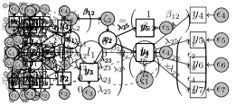
(c)

Figure 6: (a) An example model from Griliches, (1977) about the economic effects of schooling. The model has $1$ latent variable $x_{1}$ (Ability) with $4$ observed variables $y_{1}$ (IQ), $y_{2}$ (Schooling), $y_{3}$ (knowing how the world works), and $y_{4}$ (Income). (b) A slightly modified version of the model in Figure 6(a) where we add two new edges $y_{1}\rightarrow y_{2}$ and $y_{3}\rightarrow y_{4}$. (c) L2O transformed model for the equation of $y_{4}$. The transformed regression equation for $y_{4}$ is: $y_{4}\sim y_{3}+y_{2}$ but because of the transformation, the coefficient of $y_{3}$ has changed to $\lambda_{14}+\lambda_{34}$. Because of this changed coefficient, even though the equation is identified, it is not possible to estimate either $\lambda_{14}$ or $\lambda_{34}$ individually.

In the previous examples, the L2O transformation creates a new edge in the model between two observed variables that has the same path coefficient that we are interested in estimating. But if the L2O transformation adds a new edge where one already exists, the new path coefficient becomes the sum of the existing coefficient and our coefficient of interest. In such cases, certain parameters can be inestimable even if the transformed equation is identified according to the identification criteria.

In Figure 6(a), we have taken a model about the economic effects of schooling from Griliches, (1977). All parameters in the equation of $y_{4}$ are identifiable by using $y_{1}$ and $y_{2}$ as the IVs. However, we get an interesting case if we add two new edges $y_{1}\rightarrow y_{3}$ and $y_{2}\rightarrow y_{4}$ (Figure 6(b)): The L2O transformation for the equation of $y_{4}$ adds the edges $\epsilon_{3}\rightarrow y_{4}$ and $y_{3}\rightarrow y_{4}$, as shown in Figure 6(c). But since the original model already has the edge $y_{3}\rightarrow y_{4}$, the new coefficient for this edge becomes $\lambda_{14}+\lambda_{34}$. The regression equation for $y_{4}$ is still: $y_{4}\sim y_{3}+y_{2}$, and it is identified according to the instrumental set criterion as $y_{2}$ and $y_{1}$ are the IVs for the equation. But if we estimate the parameters, we will obtain values for $\lambda_{24}$ and $\lambda_{14}+\lambda_{34}$. Therefore, $\lambda_{24}$ remains identifiable in this more general case, but $\lambda_{14}$ and $\lambda_{34}$ are individually not identified. The graphical L2O approach allows us to easily visualize such cases after transformation.

7 DISCUSSION

In this paper, we showed the latent-to-observed (L2O) transformation on the RAM notation and how to use it for partial equation identification. We then gave an equivalent graphical L2O transformation which allowed us to apply graphical identification criteria developed in the DAG literature to latent variable parameters in SEMs. Combining this graphical L2O transformation with the graphical criteria for parameter identification, we arrived at a generic approach for parameter identification in SEMs. Specifically, we showed that the instrumental set criterion combined with the graphical L2O transformation is equivalent to the MIIV approach. Therefore, the graphical transformation can be used as an explicit visualization of the L2O transformation or as an alternative way to implement the MIIV approach in computer programs. To illustrate this, we have implemented the MIIV approach in the graphical-based R package dagitty (Textor et al.,, 2017) and the Python package pgmpy (Ankan and Panda,, 2015).

Our equivalence proof allows users to combine results from two largely disconnected lines of work. By combining the graphical L2O transform with other identification criteria, we obtain novel identification strategies for LVSEMs, as we have illustrated using the conditional instrumental set criterion. Other promising candidates would be auxiliary variables (Chen et al.,, 2017) and instrumental cutsets (Kumor et al.,, 2019). Conversely, the SEM literature is more developed than the graphical literature when it comes to non-Gaussian models. For example, MIIV with two-stages least squares estimation is asymptotically distribution-free (Bollen,, 1996), and our results imply that normality is not required for applying the instrumental set criterion.

Appendix A L2O Transformation for LISREL Models

In this section, we show the LISREL notation of SEMs and L2O transformation as presented in Bollen, (1996).

A.1 LISREL Notation

The LISREL notation of SEMs was first introduced in the LISREL (LInear Structural Relation) software (Joreskog and Sorbom,, 1993). This notation is based on the assumption that the models have an underlying latent structure and that the only observed variables are those that act as the measurement variables for these latents. This assumption allows us to split the set of model equations into two subsets representing: the latent model and the measurement model as follows:

$$\begin{split}\textit{Latent Model:}&\\ \eta&=\bm{B}\eta+\bm{\Gamma}\xi+\zeta\\ \textit{Measurement Model:}\\ Y&=\bm{\Lambda}_{Y}\eta+\epsilon\\ X&=\bm{\Lambda}_{X}\xi+\delta\end{split}$$ (2)

Here, $\eta$ ($\xi$) is the sets of endogenous (exogenous) latent variables, and $Y$ ($X$) is the set of observed measurement variables for $\eta$ ($\xi$). $\bm{B}$, $\bm{\Gamma}$, $\bm{\Lambda}_{Y}$, and $\bm{\Lambda}_{X}$ are the parameter matrices specifying the path coefficients in the model. $\zeta$, $\epsilon$, $\delta$ are the error vectors with the covariance matrix $\bm{\Phi}_{\zeta}$, $\bm{\Phi}_{\epsilon}$, and $\bm{\Phi}_{\delta}$ respectively. An example of an SEM in LISREL notation along with its path model representation is shown in Figure 7.

From the model equations, it appears that many possible variable relations cannot be specified directly. For example, it is not clear how to specify direct relations between two observed variables, between an observed and latent variable, or an error correlation between $\zeta$ and $\epsilon$ terms. But these relations can be modelled in the LISREL notation by making some simple modifications to the model (Bollen,, 1989). For example, for adding a direct causal relation between two observed variables, we can instead use two latent variables (with the same causal direction and path coefficient), and add the actual observed variables as single measurement variables for each latent, fixing the measurement errors for these relations to 0. This modification transforms the model into having a latent and measurement levels which can be represented in the LISREL notation.

(a)

(b)

Figure 7: Example of an SEM in LISREL notation. The parameters $\beta_{ij}$ and $\lambda_{ij}$ are the so-called path coefficients on latent-latent and latent-observed arrows, respectively. The bi-directed arrow represents a correlation between the error terms that is allowed to be nonzero, reflecting our belief that $\eta_{1}$ and $\eta_{2}$ may be correlated. (a) Model in equation form; (b) path diagram.

A.2 Algebraic L2O Transformation for LISREL Models

We now introduce the L2O transformation as shown in Bollen, (1996). Let us assume that every latent variable in the model has a unique scaling indicator that is not an indicator of any other latent variable. Then we can replace this latent variable by the difference of its scaling indicator and the scaling indicator’s error term. For instance, applying this to the latent variable $\eta_{1}$ with $y_{1}$ as its scaling indicator in the model in Figure 7 we would get

$$\eta_{1}=y_{1}-\epsilon_{1}$$

Applying this L2O transformation to all latent variables in the Equation 2 simultaneously, we get:

$$\begin{split}Y_{1}&=\bm{B}Y_{1}+\bm{\Gamma}X_{1}+\epsilon_{1}-\bm{B}\epsilon_{1}-\bm{\Gamma}\delta_{1}+\zeta\\ Y_{2}&=\bm{\Lambda}_{Y_{2}}Y_{1}-\bm{\Lambda}_{Y_{2}}\epsilon_{1}+\epsilon_{2}\\ X_{2}&=\bm{\Lambda}_{X_{2}}X_{1}-\bm{\Lambda}_{X_{2}}\delta_{1}+\delta_{2}\end{split}$$ (3)

where $X_{1}$ and $Y_{1}$ are the scaling indicators for $\eta$ and $\xi$ respectively. $X_{2}$ and $Y_{2}$ are the remaining observed variables, $X_{2}=X\setminus X_{1}$ and $Y_{2}=Y\setminus Y_{1}$. $\Lambda_{X_{2}}$ and $\Lambda_{Y_{2}}$ are submatrices of $\Lambda_{X}$ and $\Lambda_{Y}$ with only rows corresponding to $X_{2}$ and $Y_{2}$. Similarly, the error terms $\epsilon_{i}$ and $\delta_{i}$ correspond to $Y_{i}$ and $X_{i}$ respectively.

As a result of applying L2O transformation to all the latent variables, Equation 3 now only contains observed variables and each of the individual equations now resembles a standard regression equation. However, by construction, the error terms of these equations can be correlated with the covariates. This means that applying a standard least-squares estimator will provide biased estimates for the model parameters. To get unbiased estimates we can instead use an Instrumental Variable (IV) based estimator like 2-SLS (Two-Stage Least Squares) (Bollen,, 1996).

Appendix B Implied Covariance Matrix and Trek Rule

In this section, we show how the implied covariance matrix that we use in the paper is related to the model parameters. We show this both in algebraic and graphical terms.

SEMs can be rewritten to a canonical form that does not require correlations between error terms. For this, we introduce a new variable $x_{ij}$ for each upper triangular nonzero entry $\bm{\Phi}[i,j]$ and set $\beta_{x_{ij}\to x_{i}}=\beta_{x_{ij}\to x_{j}}=1$ and $\phi_{\epsilon_{ij}}=\bm{\Phi}[i,j]$. The implied covariance matrix $\bm{\Sigma}$ of a canonical SEM is given by :

$$\bm{\Sigma}=\bm{B}^{-T}\bm{\Phi}\bm{B}^{-1}$$

The trek rule (Sullivant et al.,, 2010) allows us to express covariances in SEMs in graphical terms:

$$\bm{\Sigma}[i,j]=\sum_{\text{ treks }\pi\text{ from }x_{i}\text{ to }x_{j}}\;\phi_{\pi^{\leftrightarrow}}\;\prod_{\text{arrows }k\to l\text{ on trek }\pi}\beta_{k\to l}$$ (4)

Here it is important to note that treks can contain the same nodes twice; this is required for the trek rule to work.

Appendix C Proofs

In this section, we give proofs for the theorems in the paper.

C.1 Proof of Lemma 1

Proof.

We assume that the SEM has been transformed to canonical form with no bi-directed arrows. The covariance of two variables variables $u,v\neq x_{i}$, is given by the trek rule (Equation 4). Therefore $\bm{\Sigma}[u,v]$ will be the same in $\cal G$ and $\cal G^{\prime}$ if no treks from $u$ to $v$ pass through $x_{i}$. Otherwise, let $\pi$ be a trek in ${\cal G}^{\prime}$ from $u$ to $v$ that includes $x_{i}$. There are two cases. (1) $x_{i}$ is the top of $\pi$. Then $\pi$ differs between $\cal G$ and $\cal G^{\prime}$ in the sub-trek $x_{j}\leftarrow x_{i}\to x_{k}$ with path coefficient product in $\cal G^{\prime}$ of $\alpha\beta_{x_{i}\to x_{j}}\cdot\alpha^{-2}\phi_{x_{i}}\cdot\alpha\beta_{x_{i}\to x_{k}}=\beta_{x_{i}\to x_{j}}\cdot\phi_{x_{i}}\cdot\beta_{x_{i}\to x_{k}}$ which is the same as in $\cal G$. (2) $\pi$ has a sub-trek $x_{j}\to x_{i}\to x_{k}$ with path coefficient product $\alpha\beta_{x_{j}\to x_{i}}\cdot\alpha^{-1}\beta_{x_{i}\to x_{k}}$, which again is the same as in $\cal G$. ∎

C.2 Proof of Theorem 2

Proof.

The first conditions in both criteria are equal, so we prove the equivalence between the second conditions.

$\Rightarrow$: Suppose the condition (2) of the instrumental set criterion (Definition 1) is satisfied. We need to show that no two paths $\pi_{i}$ and $\pi_{j}$ can be $t$-separated by one variable. Indeed, $\pi_{i}$ and $\pi_{j}$ can only be $t$-separated by one variable if they have a same-sided intersection $v$. But this would contradict condition (2) of Definition 1. Consequently, we need $k$ variables to $t$-separate all paths, and since these paths are a subset of the paths from $\mathbf{X}$ to $\mathbf{Z}$, we cannot $t$-separate these variable sets with fewer paths either.

$\Leftarrow$: Suppose condition (2) of the trek-based instrumental set criterion (Definition 2) is satisfied. Then there must exist sets of $k$ treks from $I$ to $X$; let $\pi_{1},\ldots,\pi_{k}$ be one such set of treks with minimal total length. No $\pi_{i}$ intersects any $\pi_{j},i\neq j,$ on the same side, otherwise we could separate all paths with $k-1$ variables. Therefore, all intersections between the $\pi_{i}$ are opposite sided. Define an ordering $\preceq$ on the $\pi_{i}$ as follows: $\pi_{i}\preceq\pi_{j}$ if $\pi_{i}$ and $\pi_{j}$ intersect at a variable $k$, which is on the left side of $\pi_{i}$ and on the right side of $\pi_{j}$ (note that $k$ cannot be the top of $\pi_{i}$ or $\pi_{j}$).

Suppose that the $\pi_{i}$ contain a cycle of length $l$ with respect to $\preceq$, that is, $\pi_{i_{1}}\preceq\ldots\preceq\pi_{i_{l}}\preceq\pi_{i_{1}}$. Then we can combine a prefix of each trek in the cycle with a suffix of the next trek to create $l$ other treks between the same variables that cannot be separated by fewer than $l$ variables, since they do not have same-sided intersections. But these new paths would be shorter than the ones on the cycle, a contradiction (see Figure 1 for an example). Hence such a cycle cannot exist, and the paths can be linearly ordered with respect to $\preceq$. Any such ordering fulfills requirement (b) of condition (2) in Definition 1.

(a)

(b)

Figure 8: (a) Paths $\pi_{1}=x_{1}\leftarrow x_{2}\leftarrow x_{3}\to z_{2}\to x_{4}$, $\pi_{2}=y_{1}\leftarrow y_{2}\leftarrow y_{3}\to x_{2}\to y_{4}$ and $\pi_{3}=z_{1}\leftarrow z_{2}\leftarrow z_{3}\to y_{2}\to z_{4}$ where $\pi_{1}\preceq\pi_{2}\preceq\pi_{3}\preceq\pi_{1}$. (b) By rearranging segments of these paths, we obtain shorter paths $\pi_{1}^{\prime}=x_{1}\leftarrow x_{2}\to y_{4}$, $\pi_{2}^{\prime}=y_{1}\leftarrow y_{2}\to z_{4}$ and $\pi_{3}^{\prime}=z_{1}\leftarrow z_{2}\to x_{4}$ between the same variables that intersect less then the original paths and therefore cannot be $t$-separated by fewer variables.

Now assume requirement (a) is violated, that is, there exist paths $\pi_{i}$ from $Z_{i}$ to $X_{i}$ and $\pi_{j}$ from $Z_{j}$ to $X_{j}$ such that $i<j$ and $Z_{j}$ also occurs on $\pi_{i}$. Then $Z_{j}$ cannot be on the left side of $\pi_{i}$ because then $Z_{j}$ would be a same-sided intersection of $\pi_{i}$ and $\pi_{j}$. But if $Z_{j}$ is on the right side of $\pi_{i}$, then $\pi_{j}\preceq\pi_{i}$, a contradiction. So requirement (a) must be fulfilled as well.

∎

C.3 Proof of Theorem 3

Proof.

Condition 3 of the algebraic instrumental set criterion holds by definition as we require the covariance matrix $\bm{\Phi}$ to be positive definite (in other words, we do not allow deterministic relations). It remains to be shown that the first two conditions of both criteria are equivalent. For condition (1), assume that some $i\in I$ is not independent of some parent $p$ of $y$, then there must be a trek from $i$ to $p$ which can be extended to $y$. Conversely, assume that there is a trek $\pi$ from $i$ to $y$ in ${\cal G}_{\overline{X}}$. Then $\pi$ ends with an arrow $p\to y$ where $p\notin X$, so $I$ is not independent of the composite error term $\epsilon$. For condition (2), the equivalence follows directly from Theorem 1. ∎

References

- Ankan and Panda, (2015) Ankan, A. and Panda, A. (2015). pgmpy: Probabilistic graphical models using python. In Proceedings of the 14th Python in Science Conference (SCIPY 2015). Citeseer.
- Bollen, (1989) Bollen, K. A. (1989). Structural Equations with Latent Variables. John Wiley & Sons, Inc.
- Bollen, (1996) Bollen, K. A. (1996). An alternative two stage least squares (2sls) estimator for latent variable equations. Psychometrika, 61(1):109–121.
- Bollen, (2012) Bollen, K. A. (2012). Instrumental variables in sociology and the social sciences. Annual Review of Sociology, 38(1):37–72.
- Bollen and Bauer, (2004) Bollen, K. A. and Bauer, D. J. (2004). Automating the selection of model-implied instrumental variables. Sociological Methods & Research, 32(4):425–452.
- Bollen et al., (2007) Bollen, K. A., Kirby, J. B., Curran, P. J., Paxton, P. M., and Chen, F. (2007). Latent variable models under misspecification: Two-stage least squares (2sls) and maximum likelihood (ML) estimators. Sociological Methods & Research, 36(1):48–86.
- Bollen et al., (2022) Bollen, K. A., Lilly, A. G., and Luo, L. (2022). Selecting scaling indicators in structural equation models (sems). Psychological Methods.
- Boomsma, (1985) Boomsma, A. (1985). Nonconvergence, improper solutions, and starting values in lisrel maximum likelihood estimation. Psychometrika, 50(2):229–242.
- Brito and Pearl, (2002) Brito, C. and Pearl, J. (2002). Generalized instrumental variables. In Proceedings of the 18th Conference in Uncertainty in Artificial Intelligence, pages 85–93.
- Chen et al., (2017) Chen, B., Kumor, D., and Bareinboim, E. (2017). Identification and model testing in linear structural equation models using auxiliary variables. In Proceedings of the 34th International Conference on Machine Learning, ICML 2017, volume 70 of Proceedings of Machine Learning Research, pages 757–766.
- Chen and Pearl, (2014) Chen, B. and Pearl, J. (2014). Graphical tools for linear structural equation modeling. Technical report.
- Fisher et al., (2019) Fisher, Z., Bollen, K., Gates, K., and Rönkkö, M. (2019). MIIVsem: Model Implied Instrumental Variable (MIIV) Estimation of Structural Equation Models. R package version 0.5.4.
- Foygel et al., (2012) Foygel, R., Draisma, J., and Drton, M. (2012). Half-trek criterion for generic identifiability of linear structural equation models. The Annals of Statistics, 40(3):1682–1713.
- Griliches, (1977) Griliches, Z. (1977). Estimating the returns to schooling: Some econometric problems. Econometrica, 45(1):1–22.
- Huang and Valtorta, (2006) Huang, Y. and Valtorta, M. (2006). Pearl’s calculus of intervention is complete. In UAI ’06, Proceedings of the 22nd Conference in Uncertainty in Artificial Intelligence.
- Joreskog and Sorbom, (1993) Joreskog, K. G. and Sorbom, D. (1993). Lisrel 8 user’s guide. Chicago: Scientific Software International.
- Kumor et al., (2019) Kumor, D., Chen, B., and Bareinboim, E. (2019). Efficient identification in linear structural causal models with instrumental cutsets. In Advances in Neural Information Processing Systems 32: Annual Conference on Neural Information Processing Systems 2019, pages 12477–12486.
- McArdle and McDonald, (1984) McArdle, J. J. and McDonald, R. P. (1984). Some algebraic properties of the reticular action model for moment structures. British Journal of Mathematical and Statistical Psychology, 37(2):234–251.
- Pearl, (2009) Pearl, J. (2009). Causality. Cambridge University Press.
- Shen and Takeuchi, (2001) Shen, B.-J. and Takeuchi, D. T. (2001). A structural model of acculturation and mental health status among chinese americans. American Journal of Community Psychology, 29(3):387–418.
- Shpitser and Pearl, (2006) Shpitser, I. and Pearl, J. (2006). Identification of joint interventional distributions in recursive semi-markovian causal models. In Proceedings, The Twenty-First National Conference on Artificial Intelligence and the Eighteenth Innovative Applications of Artificial Intelligence Conference, pages 1219–1226.
- Sullivant et al., (2010) Sullivant, S., Talaska, K., and Draisma, J. (2010). Trek separation for gaussian graphical models. The Annals of Statistics, 38(3):1665–1685.
- Tennant et al., (2019) Tennant, P. W., Harrison, W. J., Murray, E. J., Arnold, K. F., Berrie, L., Fox, M. P., Gadd, S. C., Keeble, C., Ranker, L. R., Textor, J., Tomova, G. D., Gilthorpe, M. S., and Ellison, G. T. (2019). Use of directed acyclic graphs (DAGs) in applied health research: review and recommendations.
- Textor et al., (2017) Textor, J., van der Zander, B., Gilthorpe, M. S., Liśkiewicz, M., and Ellison, G. T. (2017). Robust causal inference using directed acyclic graphs: the r package ‘dagitty’. International Journal of Epidemiology, page dyw341.
- van der Zander and Liśkiewicz, (2016) van der Zander, B. and Liśkiewicz, M. (2016). On searching for generalized instrumental variables. In Proceedings of the 19th International Conference on Artificial Intelligence and Statistics, AISTATS 2016, Cadiz, Spain, May 9-11, 2016, volume 51 of JMLR Workshop and Conference Proceedings, pages 1214–1222.