Closed form solution and transmutation operators for Schrödinger equations with finitely many $\delta$-interactions

Abstract

A closed form solution for the one-dimensional Schrödinger equation with a finite number of $\delta$-interactions

$$\mathbf{L}_{q,\mathfrak{I}_{N}}y:=-y^{\prime\prime}+\left(q(x)+\sum_{k=1}^{N}\alpha_{k}\delta(x-x_{k})\right)y=\lambda y,\quad 0<x<b,\;\lambda\in\mathbb{C}$$

is presented in terms of the solution of the unperturbed equation

$$\mathbf{L}_{q}y:=-y^{\prime\prime}+q(x)y=\lambda y,\quad 0<x<b,\;\lambda\in\mathbb{C}$$

and a corresponding transmutation operator $\mathbf{T}_{\mathfrak{I}_{N}}^{f}$ is obtained in the form of a Volterra integral operator. With the aid of the spectral parameter power series method, a practical construction of the image of the transmutation operator on a dense set is presented, and it is proved that the operator $\mathbf{T}_{\mathfrak{I}_{N}}^{f}$ transmutes the second derivative into the Schrödinger operator $\mathbf{L}_{q,\mathfrak{I}_{N}}$ on a Sobolev space $H^{2}$. A Fourier-Legendre series representation for the integral transmutation kernel is developed, from which a new representation for the solutions and their derivatives, in the form of a Neumann series of Bessel functions, is derived.

Keywords: One-dimensional Schrödinger equation, point interactions, transmutation operator, Fourier-Legendre series, Neumann series of Bessel functions.

MSC Classification: 34A25; 34A45; 46F10; 47G10; 81Q05.

1 Introduction

We consider the one-dimensional Schrödinger equation with a finite number of $\delta$-interactions

$$-y^{\prime\prime}+\left(q(x)+\sum_{k=1}^{N}\alpha_{k}\delta(x-x_{k})\right)y=\lambda y,\quad 0<x<b,\;\lambda\in\mathbb{C},$$ (1)

where $q\in L_{2}(0,b)$ is a complex valued function, $\delta(x)$ is the Dirac delta distribution, $0<x_{1}<x_{2}<\dots<x_{N}<b$ and $\alpha_{1},\dots,\alpha_{N}\in\mathbb{C}\setminus\{0\}$. Schrödinger equations with distributional coefficients supported on a set of measure zero naturally appear in various problems of mathematical physics [3, 4, 5, 6, 16, 44] and have been studied in a considerable number of publications and from different perspectives. In general terms, Eq. (1) can be interpreted as a regular equation, i.e., with the regular potential $q\in L_{2}(0,b)$, whose solutions are continuous and such that their first derivatives satisfy the jump condition $y^{\prime}(x_{k}+)-y^{\prime}(x_{k}-)=\alpha_{k}y(x_{k})$ at special points [25, 26]. Another approach consists in considering the interval $[0,b]$ as a quantum graph whose edges are the segments $[x_{k},x_{k+1}]$, $k=0,\dots,N$, (setting $x_{0}=0$, $x_{N+1}=b$), and the Schrödinger operator with the regular potential $q$ as an unbounded operator on the direct sum $\bigoplus_{k=0}^{N}H^{2}(x_{k},x_{k+1})$, with the domain given by the families $(y_{k})_{k=0}^{N}$ that satisfy the condition of continuity $y_{k}(x_{k}-)=y_{k+1}(x_{k}+)$ and the jump condition for the derivative $y_{k+1}^{\prime}(x_{k}+)-y_{k}^{\prime}(x_{k}-)=\alpha_{k}y_{k}(x_{k})$ for $k=1,\dots N$ (see, e.g., [18, 34, 35]). This condition for the derivative is known in the bibliography of quantum graphs as the $\delta$-type condition [9]. Yet another approach implies a regularization of the Schrodinger operator with point interactions, that is, finding a subdomain of the Hilbert space $L_{2}(0,b)$, where the operator defines a function in $L_{2}(0,b)$. For this, note that the potential $q(x)+\sum_{k=1}^{N}\alpha_{k}\delta(x-x_{k})$ defines a functional that belongs to the Sobolev space $H^{-1}(0,b)$. In [11, 20, 23, 42] these forms of regularization have been studied, rewriting the operator by means of a factorization that involves a primitive $\sigma$ of the potential.

Theory of transmutation operators, also called transformation operators, is a widely used tool in studying differential equations and spectral problems (see, e.g., [8, 29, 36, 39, 43]), and it is especially well developed for Schrödinger equations with regular potentials. It is known that under certain general conditions on the potential $q$ the transmutation operator transmuting the second derivative into the Schrödinger operator can be realized in the form of a Volterra integral operator of the second kind, whose kernel can be obtained by solving a Goursat problem for the Klein-Gordon equation with a variable coefficient [14, 36, 39]. Furthermore, functional series representations of the transmutation kernel have been constructed and used for solving direct and inverse Sturm-Liouville problems [29, 30]. For Schrödinger equations with $\delta$-point interactions, there exist results about equations with a single point interaction and discontinuous conditions $y(x_{1}+)=ay(x_{1}-)$, $y^{\prime}(x_{1}+)=\frac{1}{a}y^{\prime}(x_{1}-)+dy(x_{1}-)$, $a,b>0$ (see [22, 46]), and for equations in which the spectral parameter is also present in the jump condition (see [1, 37, 38]). Transmutation operators have also been studied for equations with distributional coefficients belonging to the $H^{-1}$-Sobolev space in [11, 23, 42]. In [14], the possibility of extending the action of the transmutation operator for an $L_{1}$-potential to the space of generalized functions $\mathscr{D}^{\prime}$, was studied.

The aim of this work is to present a construction of a transmutation operator for the Schrödinger equation with a finite number of point interactions. The transmutation operator appears in the form of a Volterra integral operator, and with its aid we derive analytical series representations for solutions of (1). For this purpose, we obtain a closed form of the general solution of (1). From it, the construction of the transmutation operator is deduced, where the transmutation kernel is ensembled from the convolutions of the kernels of certain solutions of the regular equation (with the potential $q$), in a finite number of steps. Next, the spectral parameter power series (SPPS) method is developed for Eq. (1). The SPPS method was developed for continuous ([27, 31]) and $L_{1}$-potentials ([10]), and it has been used in a piecewise manner for solving spectral problems for equations with a finite number of point interactions in [6, 7, 41]. Following [15], we use the SPPS method to obtain an explicit construction of the image of the transmutation operator acting on polynomials. Similarly to the case of a regular potential [30], we obtain a representation of the transmutation kernel as a Fourier series in terms of Legendre polynomials and as a corollary, a representation for the solutions of equation (1) in terms of a Neumann series of Bessel functions. Similar representations are obtained for the derivatives of the solutions. It is worth mentioning that the methods based on Fourier-Legendre representations and Neumann series of Bessel functions have shown to be an effective tool in solving direct and inverse spectral problems for equations with regular potentials, see, e.g., [29, 30, 33].

In Section 2, basic properties of the solutions of (1) are compiled, studying the equation as a distributionional sense in $\mathscr{D}^{\prime}(0,b)$ and deducing properties of its regular solutions. Section 3 presents the construction of the closed form solution of (1). In Section 4, the construction of the transmutation operator and the main properties of the transmutation kernel are developed. In Section 5, the SPPS method is presented, with the mapping and transmutation properties of the transmutation operator. Section 6 presents the Fourier-Legendre series representations for the transmutation kernels and the Neumann series of Bessel functions representations for solutions of (1), and a recursive integral relation for the Fourier-Legendre coefficients is obtained. Finally, in Section 7, integral and Neumann series of Bessel functions representations for the derivatives of the solutions are presented.

2 Problem setting and properties of the solutions

We use the standard notation $W^{k,p}(0,b)$ ($b>0$) for the Sobolev space of functions in $L_{p}(0,b)$ that have their first $k$ weak derivatives in $L_{p}(0,b)$, $1\leqslant p\leqslant\infty$ and $k\in\mathbb{N}$. When $p=2$, we denote $W^{k,2}(0,b)=H^{k}(0,b)$. We have that $W^{1,1}(0,b)=AC[0,b]$, and $W^{1,\infty}(0,b)$ is precisely the class of Lipschitz continuous functions in $[0,b]$ (see [12, Ch. 8]). The class of smooth functions with compact support in $(0,b)$ is denoted by $C_{0}^{\infty}(0,b)$, then we define $W_{0}^{1,p}(0,b)=\overline{C_{0}^{\infty}(0,b)}^{W^{1,p}}$ and $H_{0}^{1}(0,b)=W_{0}^{1,2}(0,b)$. Denote the dual space of $H^{1}_{0}(0,b)$ by $H^{-1}(0,b)$. By $L_{2,loc}(0,b)$ we denote the class of measurable functions $f:(0,b)\rightarrow\mathbb{C}$ such that $\int_{\alpha}^{\beta}|f(x)|^{2}dx<\infty$ for all subintervals $[\alpha,\beta]\subset(0,b)$.

The characteristic function of an interval $[A,B]\subset\mathbb{R}$ is denoted by $\chi_{[A,B]}(t)$. In order to simplify the notation, for the case of a symmetric interval $[-A,A]$, we simply write $\chi_{A}$. The Heaviside function is given by $H(t)=\chi_{(0,\infty)}(t)$. The lateral limits of the function $f$ at the point $\xi$ are denoted by $f(\xi\pm)=\lim_{x\rightarrow\xi{\pm}}f(x)$. We use the notation $\mathbb{N}_{0}=\mathbb{N}\cup\{0\}$. The space of distributions (generalized functions) over $C_{0}^{\infty}(0,b)$ is denoted by $\mathscr{D}^{\prime}(0,b)$, and the value of a distribution $f\in\mathscr{D}^{\prime}(0,b)$ at $\phi\in C_{0}^{\infty}(0,b)$ is denoted by $(f,\phi)_{C_{0}^{\infty}(0,b)}$.

Let $N\in\mathbb{N}$ and consider a partition $0<x_{1}<\dots<x_{N}<b$ and the numbers $\alpha_{1},\dots,\alpha_{N}\in\mathbb{C}\setminus\{0\}$. The set $\mathfrak{I}_{N}=\{(x_{j},\alpha_{j})\}_{j=1}^{N}$ contains the information about the point interactions of Eq. (1). Denote

$$q_{\delta,\mathfrak{I}_{N}}(x):=\sum_{k=1}^{N}\alpha_{k}\delta(x-x_{k}),\quad\mathbf{L}_{q}:=-\frac{d^{2}}{dx^{2}}+q(x),\quad\mathbf{L}_{q,\mathfrak{I}_{N}}:=\mathbf{L}_{q}+q_{\delta,\mathfrak{I}_{N}}(x).$$

For $u\in L_{2,loc}(0,b)$, $\mathbf{L}_{q,\mathfrak{I}_{N}}u$ defines a distribution in $\mathscr{D}^{\prime}(0,b)$ as follows

$$(\mathbf{L}_{q,\mathfrak{I}_{N}}u,\phi)_{C_{0}^{\infty}(0,b)}:=\int_{0}^{b}u(x)\mathbf{L}_{q}\phi(x)dx+\sum_{k=1}^{N}\alpha_{k}u(x_{k})\phi(x_{k})\quad\mbox{for }\,\phi\in C_{0}^{\infty}(0,b).$$

Note that the function $u$ must be well defined at the points $x_{k}$, $k=1,\dots,N$. Actually, for a function $u\in H^{1}(0,b)$, the distribution $\mathbf{L}_{q,\mathfrak{I}_{N}}u$ can be extended to a functional in $H^{-1}(0,b)$ as follows

$$(\mathbf{L}_{q,\mathfrak{I}_{N}}u,v)_{H_{0}^{1}(0,b)}:=\int_{0}^{b}\{u^{\prime}(x)v^{\prime}(x)+q(x)u(x)v(x)\}dx+\sum_{k=1}^{N}\alpha_{k}u(x_{k})v(x_{k})\quad\mbox{for }\,v\in H_{0}^{1}(0,b).$$

We say that a distribution $F\in\mathscr{D}^{\prime}(0,b)$ is $L_{2}$-regular, if there exists a function $g\in L_{2}(0,b)$ such that $(F,\phi)_{C_{0}^{\infty}(0,b)}=(g,\phi)_{C_{0}^{\infty}(0,b)}:=\int_{0}^{b}g(x)\phi(x)dx$ for all $\phi\in{C_{0}^{\infty}(0,b)}$.

Denote $x_{0}=0$, $x_{N+1}=b$. We recall the following characterization of functions $u\in L_{2,loc}(0,b)$ for which $\mathbf{L}_{q,\mathfrak{I}_{N}}u$ is $L_{2}$-regular.

Proposition 1

If $u\in L_{2,loc}(0,b)$, then the distribution $\mathbf{L}_{q,\mathfrak{I}_{N}}u$ is $L_{2}$-regular iff the following conditions hold.

1. For each $k=0,\dots,N$, $u|_{(x_{k},x_{k+1})}\in H^{2}(x_{k},x_{k+1})$.

2. $u\in AC[0,b]$.

3. The discontinuities of the derivative $u^{\prime}$ are located at the points $x_{k}$, $k=1,\dots,N$, and the jumps are given by

   $$u^{\prime}(x_{k}+)-u^{\prime}(x_{k}-)=\alpha_{j}u(x_{k})\quad\mbox{for }k=1,\cdots,N.$$ (2)

In such case,

$$(\mathbf{L}_{q,\mathfrak{I}_{N}}u,\phi)_{C_{0}^{\infty}(0,b)}=(\mathbf{L}_{q}u,\phi)_{C_{0}^{\infty}(0,b)}\quad\mbox{for all }\phi\in{C_{0}^{\infty}(0,b)}.$$ (3)

Proof. Suppose that $\mathbf{L}_{q,\mathfrak{I}_{N}}u$ is $L_{2}$-regular. Then there exists $g\in L_{2}(0,b)$ such that

$$(\mathbf{L}_{q,\mathfrak{I}_{N}}u,\phi)_{C_{0}^{\infty}(0,b)}=(g,\phi)_{C_{0}^{\infty}(0,b)}\quad\mbox{for all }\phi\in{C_{0}^{\infty}(0,b)}.$$ (4)

1. Fix $k\in\{1,\dots,N-1\}$. Take a test function $\phi\in C_{0}^{\infty}(0,b)$ with $\operatorname{Supp}(\phi)\subset(x_{k},x_{k+1})$. Hence

   $$\int_{x_{k}}^{x_{k+1}}g(x)\phi(x)dx=(\mathbf{L}_{q,\mathfrak{I}_{N}}u,\phi)_{C_{0}^{\infty}(0,b)}=\int_{x_{k}}^{x_{k+1}}u(x)\mathbf{L}_{q}\phi(x)dx,$$ (5)

   because $\phi(x_{j})=0$ for $j=1,\dots,N$. From (5) we obtain

   $$\int_{x_{k}}^{x_{k+1}}u(x)\phi^{\prime\prime}(x)dx=\int_{x_{k}}^{x_{k+1}}\{q(x)u(x)-g(x)\}\phi(x)dx.$$

   Set $v(x)=\int_{0}^{x}\int_{0}^{t}\{q(s)u(s)-g(s)\}dsdt$. Hence $v\in W^{2,1}(x_{j},x_{j+1})$, $v^{\prime\prime}(x)=q(x)u(x)-g(x)$ a.e. $x\in(x_{j},x_{j+1})$, and we get the equality

   $$\int_{x_{k}}^{x_{k+1}}(u(x)-v(x))\phi^{\prime\prime}(x)dx=0\quad\forall\phi\in C_{0}^{\infty}(x_{k},x_{k+1}).$$ (6)

   Equality (6) implies that $u(x)=v(x)+Ax+B$ a.e. $x\in(x_{k},x_{k+1})$ for some constants $A$ and $B$ ([45, pp. 85]). In consequence $u\in W^{2,1}(x_{k},x_{k+1})$ and

   $$-u^{\prime\prime}(x)+q(x)u(x)=g(x)\quad\mbox{a.e. }x\in(x_{k},x_{k+1}).$$ (7)

   Furthermore, $u\in C[x_{k},x_{k+1}]$, hence $qu\in L_{2}(x_{k},x_{k+1})$ and then $u^{\prime\prime}=qu-g\in L_{2}(x_{k},x_{k+1})$. In this way $u|_{(x_{k},x_{k+1})}\in H^{2}(x_{k},x_{k+1})$.

   Now take $\varepsilon>0$ and an arbitrary $\phi\in C_{0}^{\infty}(\varepsilon,x_{1})$. We have that

   $$(\mathbf{L}_{q,\mathfrak{I}_{N}}u,\phi)_{C_{0}^{\infty}(0,b)}=\int_{\varepsilon}^{x_{1}}\{-u(x)\phi^{\prime\prime}(x)+q(x)u(x)\phi(x)\}dx=\int_{\varepsilon}^{x_{1}}g(x)\phi(x)dx.$$

   Applying the same procedure as in the previous case we obtain that $u\in H^{2}(\varepsilon,x_{1})$ and satisfies Eq. (7) in the interval $(\varepsilon,x_{1})$. Since $\varepsilon$ is arbitrary, we conclude that $u$ satisfies (7) for a.e. $x\in(0,x_{1})$. Since $q,g\in L_{2}(0,x_{1})$, then $u|_{(0,x_{1})}\in H^{2}(0,x_{1})$ (see [47, Th. 3.4]). The proof for the interval $(x_{N},b)$ is analogous.

   Since $u\in C^{1}[x_{k},x_{k+1}]$, $k=0,\dots,N$, the following equality is valid (see formula (6) from [24, pp. 100])

   $$\int_{0}^{b}u(x)\phi^{\prime\prime}(x)dx =\sum_{k=1}^{N}\left\{u^{\prime}(x_{k}+)-u^{\prime}(x_{k}-)\right\}\phi(x_{k})$$ (8)

   $$\quad-\sum_{k=1}^{N}\left\{u(x_{k}+)-u(x_{k}-)\right\}\phi^{\prime}(x_{k})+\int_{0}^{b}u^{\prime\prime}(x)\phi(x)dx,\qquad\forall\phi\in C_{0}^{\infty}(0,b).$$

   Fix $k\in\{1,\cdots,N\}$ arbitrary and take $\varepsilon>0$ small enough such that $(x_{k}-\varepsilon,x_{k}+\varepsilon)\subset(x_{k-1},x_{k+1})$. Choose a cut-off function $\psi\in C_{0}^{\infty}(x_{k}-\varepsilon,x_{k}+\varepsilon)$ satisfying $0\leqslant\psi\leqslant 1$ on $(x_{k}-\varepsilon,x_{k}+\varepsilon)$ and $\psi(x)=1$ for $x\in(x_{k}-\frac{\varepsilon}{3},x_{k}+\frac{\varepsilon}{3})$.

2. By statement 1, it is enough to show that $u(x_{k}+)=u(x_{k}-)$. Set
   $\phi(x)=(x-x_{k})\psi(x)$, in such a way that $\phi(x_{k})=0$ and $\phi^{\prime}(x_{k})=1$. Hence

   $$(\mathbf{L}_{q,\mathfrak{I}_{N}}u,\phi)_{C_{0}^{\infty}(0,b)}=\int_{x_{k}-\varepsilon}^{x_{k}+\varepsilon}u(x)\mathbf{L}_{q}\phi(x)dx.$$

   By (8) we have

   $$\int_{x_{k}-\varepsilon}^{x_{k}+\varepsilon}u(x)\phi^{\prime\prime}(x)dx=u(x_{k}-)-u(x_{k}+)+\int_{x_{k}-\varepsilon}^{x_{k}+\varepsilon}u^{\prime\prime}(x)\phi(x)dx,$$

   because $\phi(x_{k})=0$ and $\phi^{\prime}(x_{k})=1$. Since $u$ satisfies (4), we have

   $$\int_{x_{k}-\varepsilon}^{x_{k}+\varepsilon}(\mathbf{L}_{q}u(x)-g(x))\phi(x)dx+u(x_{k}+)-u(x_{k}-)=0.$$

   By statement 1, $\mathbf{L}_{q}u=g$ on both intervals $(x_{k-1},x_{k})$, $(x_{k},x_{k+1})$. Then we obtain that $u(x_{k}+)-u(x_{k}-)$=0.

3. Now take $\psi$ as the test function. Hence

   $$(\mathbf{L}_{q,\mathfrak{I}_{N}}u,\psi)_{C_{0}^{\infty}(0,b)}=\int_{x_{k}-\varepsilon}^{x_{k}+\varepsilon}u(x)\mathbf{L}_{q}\psi(x)dx+\alpha_{k}u(x_{k}),$$

   because $\operatorname{Supp}(\psi)\subset(x_{k}-\varepsilon,x_{k}+\varepsilon)$ and $\psi\equiv 1$ on $(x_{k}-\frac{\varepsilon}{3},x_{k}+\frac{\varepsilon}{3})$. On the other hand, by (8) we obtain

   $$\int_{x_{k}-\varepsilon}^{x_{k}+\varepsilon}u(x)\psi^{\prime\prime}(x)dx=u^{\prime}(x_{k}+)-u^{\prime}(x_{k}-)+\int_{x_{k}-\varepsilon}^{x_{k}+\varepsilon}u^{\prime\prime}(x)\psi(x)dx,$$

   because $\psi^{\prime}(x_{k})=0$. Thus, by (4) we have

   $$\int_{x_{k}-\varepsilon}^{x_{k}+\varepsilon}(\mathbf{L}_{q}u(x)-g(x))\psi(x)dx+u^{\prime}(x_{k}-)-u^{\prime}(x_{k}+)+\alpha_{k}u(x_{k})=0.$$

   Again, by statement 1, we obtain (2).

Reciprocally, if $u$ satisfies conditions 1,2 and 3, equality (8) implies (3). By condition 1, $\mathbf{L}_{q,\mathfrak{I}_{N}}u$ is $L_{2}$-regular.   

Definition 2

The $L_{2}$-regularization domain of $\mathbf{L}_{q,\mathfrak{I}_{N}}$, denoted by $\mathcal{D}_{2}\left(\mathbf{L}_{q,\mathfrak{I}_{N}}\right)$, is the set of all functions $u\in L_{2,loc}(0,b)$ satisfying conditions 1,2 and 3 of Proposition 1.

If $u\in L_{2,loc}(0,b)$ is a solution of (1), then $\mathbf{L}_{q-\lambda,\mathfrak{I}_{N}}u$ equals the regular distribution zero. Then we have the next characterization.

Corollary 3

A function $u\in L_{2,loc}(0,b)$ is a solution of Eq. (1) iff $u\in\mathcal{D}_{2}\left(\mathbf{L}_{q,\mathfrak{I}_{N}}\right)$ and for each $k=0,\dots,N$, the restriction $u|_{(x_{k},x_{k+1})}$ is a solution of the regular Schrödinger equation

$$-y^{\prime\prime}(x)+q(x)y(x)=\lambda y(x)\quad\mbox{for }x_{k}<x<x_{k+1}.$$ (9)

Remark 4

Let $f\in\mathcal{D}_{2}\left(\mathbf{L}_{q,\mathfrak{I}_{N}}\right)$. Given $g\in C^{1}[0,b]$, we have

$$(fg)^{\prime}(x_{k}+)-(fg)^{\prime}(x_{k}-) =f^{\prime}(x_{k}+)g(x_{k})+f(x_{k})g^{\prime}(x_{k}+)-f^{\prime}(x_{k}-)g(x_{k})-f(x_{k})g^{\prime}(x_{k}-)$$

$$=\left[f^{\prime}(x_{k}+)-f^{\prime}(x_{k}-)\right]g(x_{k})=\alpha_{k}f(x_{k})g(x_{k})$$

for $k=1,\dots,N$. In particular, $fg\in\mathcal{D}_{2}\left(\mathbf{L}_{q,\mathfrak{I}_{N}}\right)$ for $g\in H^{2}(0,b)$.

Remark 5

Let $u_{0},u_{1}\in\mathbb{C}$. Consider the Cauchy problem

$$\begin{cases}\mathbf{L}_{q,\mathfrak{I}_{N}}u(x)=\lambda u(x),\quad 0<x<b,\\ u(0)=u_{0},\;u^{\prime}(0)=u_{1}.\end{cases}$$ (10)

If the solution of the problem exists, it must be unique. It is enough to show the assertion for $u_{0}=u_{1}=0$. Indeed, if $w$ is a solution of such problem, by Corollary 3, $w$ is a solution of (9) on $(0,x_{1})$ satisfying $w(0)=w^{\prime}(0)=0$. Hence $w\equiv 0$ on $[0,x_{1}]$. By the continuity of $w$ and condition (2), we have $w(x_{1})=w^{\prime}(x_{1}-)=0$. Hence $w$ is a solution of (9) satisfying these homogeneous conditions. Thus, $w\equiv 0$ on $[x_{1},x_{2}]$. By continuing the process until the points $x_{k}$ are exhausted, we arrive at the solution $w\equiv 0$ on the whole segment $[0,b]$.

The uniqueness of the Cauchy problem with conditions $u(b)=u_{0}$, $u^{\prime}(b)=u_{1}$ is proved in a similar way.

Remark 6

Suppose that $u_{0}=u_{0}(\lambda)$ and $u_{1}=u_{1}(\lambda)$ are entire functions of $\lambda$ and denote by $u(\lambda,x)$ the corresponding unique solution of (10). Since $u$ is the solution of the Cauchy problem $\mathbf{L}_{q}u=\lambda u$ on $(0,x_{1})$ with the initial conditions $u(\lambda,0)=u_{1}(\lambda)$, $u^{\prime}(\lambda,0)=u_{1}(\lambda)$, both $u(\lambda,x)$ and $u^{\prime}(\lambda,x+)$ are entire functions for any $x\in[0,x_{1}]$ (this is a consequence of [47, Th. 3.9] and [10, Th. 7]). Hence $u^{\prime}(\lambda,x_{1}-)=u^{\prime}(\lambda,x_{1}+)-\alpha_{1}u(\lambda,x_{1})$ is entire in $\lambda$. Since $u$ is the solution of the Cauchy problem $\mathbf{L}_{q}u=\lambda u$ on $(x_{1},x_{2})$ with initial conditions $u(\lambda,x_{1})$ and $u^{\prime}(\lambda,x_{1}+)$, we have that $u(\lambda,x)$ and $u^{\prime}(\lambda,x+)$ are entire functions for $x\in[x_{1},x_{2}]$. By continuing the process we prove this assertion for all $x\in[0,b]$.

3 Closed form solution

In what follows, denote the square root of $\lambda$ by $\rho$, so $\lambda=\rho^{2}$, $\rho\in\mathbb{C}$. For each $k\in\{1,\cdots,N\}$ let $\widehat{s}_{k}(\rho,x)$ be the unique solution of the Cauchy problem

$$\begin{cases}-\widehat{s}_{k}^{\prime\prime}(\rho,x)+q(x+x_{k})\widehat{s}_{k}(\rho,x)=\rho^{2}\widehat{s}_{k}(\rho,x)\quad\mbox{ for }0<x<b-x_{k},\\ \widehat{s}_{k}(\rho,0)=0,\;\widehat{s}_{k}^{\prime}(\rho,0)=1.\end{cases}$$ (11)

In this way, $\widehat{s}_{k}(\rho,x-x_{k})$ is a solution of $\mathbf{L}_{q}u=\rho^{2}u$ on $(x_{k},b)$ with initial conditions $u(x_{k})=0$, $u^{\prime}(x_{k})=1$. According to [45, Ch. 3, Sec. 6.3], $(\mathbf{L}_{q}-\rho^{2})\left(H(x-x_{k})\widehat{s}_{k}(\rho,x-x_{k})\right)=-\delta(x-x_{k})$ for $x_{k}<x<b$.

We denote by $\mathcal{J}_{N}$ the set of finite sequences $J=(j_{1},\dots,j_{l})$ with $1<l\leqslant N$, $\{j_{1},\dots,j_{l}\}\subset\{1,\dots,N\}$ and $j_{1}<\cdots<j_{l}$. Given $J\in\mathcal{J}_{N}$, the length of $J$ is denoted by $|J|$ and we define $\alpha_{J}:=\alpha_{j_{1}}\cdots\alpha_{j_{|J|}}$.

Theorem 7

Given $u_{0},u_{1}\in\mathbb{C}$, the unique solution $\displaystyle u_{\mathfrak{I}_{N}}\in\mathcal{D}_{2}\left(\mathbf{L}_{q,\mathfrak{I}_{N}}\right)$ of the Cauchy problem (10) has the form

$$u_{\mathfrak{I}_{N}}(\rho,x) =\widetilde{u}(\rho,x)+\sum_{k=1}^{N}\alpha_{k}\widetilde{u}(\rho,x_{k})H(x-x_{k})\widehat{s}_{k}(\rho,x-x_{k})$$

$$\;\;\;\;+\sum_{J\in\mathcal{J}_{N}}\alpha_{J}H(x-x_{j_{|J|}})\widetilde{u}(\rho,x_{j_{1}})\left(\prod_{l=1}^{|J|-1}\widehat{s}_{j_{l}}(\rho,x_{j_{l+1}}-x_{j_{l}})\right)\widehat{s}_{j_{|J|}}(\rho,x-x_{j_{|J|}}),$$ (12)

where $\widetilde{u}(\rho,x)$ is the unique solution of the regular Schrödinger equation

$$\mathbf{L}_{q}\widetilde{u}(\rho,x)=\rho^{2}\widetilde{u}(\rho,x),\quad 0<x<b,$$ (13)

satisfying the initial conditions $\widetilde{u}(\rho,0)=u_{1},\;\widetilde{u}^{\prime}(\rho,0)=u_{1}$.

Proof. The proof is by induction on $N$. For $N=1$, the proposed solution has the form

$$u_{\mathfrak{I}_{1}}(\rho,x)=\widetilde{u}(\rho,x)+\alpha_{1}H(x-x_{1})\widetilde{u}(\rho,x_{1})\widehat{s}_{1}(\rho,x-x_{1}).$$

Note that $u_{\mathfrak{I}_{1}}(\rho,x)$ is continuous, and $u_{\mathfrak{I}_{1}}(\rho,x_{1})=\widetilde{u}(\rho,x_{1})$. Hence

$$(\mathbf{L}_{q}-\rho^{2})u_{\mathfrak{I}_{1}}(\rho,x)=\alpha_{1}\widetilde{u}(\rho,x_{1})(\mathbf{L}_{q}-\rho^{2})\left(H(x-x_{1})\widehat{s}_{1}(\rho,x-x_{1})\right)=-\alpha_{1}\widetilde{u}(\rho,x_{1})\delta(x-x_{1}),$$

that is, $u_{\mathfrak{I}_{1}}(\rho,x)$ is a solution of (1) with $N=1$. Suppose the result is valid for $N$. Let $u_{\mathfrak{I}_{N+1}}(\rho,x)$ be the proposed solution given by formula (12). It is clear that $u_{\mathfrak{I}_{N+1}}(\rho,\cdot)|_{(x_{k},x_{k+1})}\in H^{2}(x_{k},x_{k+1})$, $k=0,\cdots,N$, $u_{\mathfrak{I}_{N+1}}(\rho,x)$ is a solution of (9) on each interval $(x_{k},x_{k+1})$, $k=0,\dots,N+1$, and $u_{\mathfrak{I}_{N+1}}^{(j)}(\rho,0)=\widetilde{u}^{(j)}(\rho,0)=u_{j}$, $j=0,1$. Furthermore, we can write

$$u_{\mathfrak{I}_{N+1}}(\rho,x)=u_{\mathfrak{I}_{N}}(\rho,x)+H(x-x_{N+1})f_{N}(\rho,x),$$

where $\mathfrak{I}_{N}=\mathfrak{I}_{N+1}\setminus\{(x_{N+1},\alpha_{N+1})\}$, $u_{\mathfrak{J}_{N}}(\rho,x)$ is the proposed solution for the interactions $\mathfrak{I}_{N}$, and the function $f_{N}(\rho,x)$ is given by

$$f_{N}(\rho,x) =\alpha_{N+1}\widetilde{u}(\rho,x_{N+1})\widehat{s}_{N+1}(x-x_{N+1})$$

$$\quad+\sum_{\overset{J\in\mathcal{J}_{N+1}}{j_{|J|}=N+1}}\alpha_{J}\widetilde{u}(\rho,x_{j_{1}})\left(\prod_{l=1}^{|J|-1}\widehat{s}_{j_{l}}(\rho,x_{j_{l+1}}-x_{j_{l}})\right)\widehat{s}_{N+1}(\rho,x-x_{N+1}),$$

where the sum is taken over all the sequences $J=(j_{1},\dots,j_{|J|})\in\mathcal{J}_{N}$ with $j_{|J|}=N+1$. From this representation we obtain $u_{\mathfrak{I}_{N+1}}(\rho,x_{N+1}\pm)=u_{\mathfrak{I}_{N}}(\rho,x_{N+1})$ and hence $u_{\mathfrak{I}_{N+1}}\in AC[0,b]$. By the induction hypothesis, $u_{\mathfrak{I}_{N}}(\rho,x)$ is the solution of (1) for $N$, then in order to show that $u_{\mathfrak{I}_{N+1}}(\rho,x)$ is the solution for $N+1$ it is enough to show that $(\mathbf{L}_{q}-\rho^{2})\hat{f}_{N}(\rho,x)=-\alpha_{N}u_{N}(x_{N+1})\delta(x-x_{N+1})$, where $\hat{f}_{N}(\rho,x)=H(x-x_{N+1})f_{N}(\rho,x)$. Indeed, we have

$$(\rho^{2}-\mathbf{L}_{q})\hat{f}_{N}(\rho,x) =\alpha_{N+1}\widetilde{u}(\rho,x_{N+1})\delta(x-x_{N+1})+$$

$$\quad\;+\sum_{\overset{J\in\mathcal{J}_{N+1}}{j_{|J|}=N+1}}\alpha_{J}\widetilde{u}(\rho,x_{j_{1}})\left(\prod_{l=1}^{|J|-1}\widehat{s}_{j_{l}}(\rho,x_{j_{l+1}}-x_{j_{l}})\right)\delta(x-x_{N+1})$$

$$=\alpha_{N+1}\delta(x-x_{N+1})\Bigg{[}\widetilde{u}(\rho,x_{N+1})+\sum_{k=1}^{N}\alpha_{k}\widetilde{u}(\rho,x_{N+1})\widehat{s}_{k}(\rho,x_{N+1}-x_{k})$$

$$\quad\;\;\,+\sum_{J\in\mathcal{J}_{N}}\alpha_{J}\widetilde{u}(\rho,x_{j_{1}})\left(\prod_{l=1}^{|J|-1}\widehat{s}_{j_{l}}(\rho,x_{j_{l+1}}-x_{j_{l}})\right)\widehat{s}_{j_{|J|}}(\rho,x_{N+1}-x_{j_{|J|}})\Bigg{]}$$

$$=\alpha_{N+1}u_{\mathfrak{I}_{N}}(\rho,x_{N+1})\delta(x-x_{N+1})=\alpha_{N+1}u_{\mathfrak{I}_{N+1}}(\rho,x_{N+1})\delta(x-x_{N+1}),$$

where the second equality is due to the fact that

$$\{J\in\mathcal{J}_{N+1}\,|\,j_{|J|}=N+1\}=\{(J^{\prime},N+1)\,|\,J^{\prime}\in\mathcal{J}_{N}\}\cup\{(j,N+1)\}_{j=1}^{N}.$$

Hence $u_{\mathfrak{I}_{N+1}}(\rho,x)$ is the solution of the Cauchy problem.   

Example 8

Consider the case $q\equiv 0$. Denote by $e_{\mathfrak{I}_{N}}^{0}(\rho,x)$ the unique solution of

$$-y^{\prime\prime}+\left(\sum_{k=1}^{N}\alpha_{k}\delta(x-x_{k})\right)y=\rho^{2}y,\quad 0<x<b,$$ (14)

satisfying $e_{\mathfrak{I}_{N}}^{0}(\rho,0)=1$, $e_{\mathfrak{I}_{N}}^{0}(\rho,0)=i\rho$. In this case we have $\widehat{s}_{k}(\rho,x)=\frac{\sin(\rho x)}{\rho}$ for $k=1,\dots,N$. Hence, according to Theorem 7, the solution $e_{\mathfrak{I}_{N}}^{0}(\rho,x)$ has the form

$$e_{\mathfrak{I}_{N}}^{0}(\rho,x) =e^{i\rho x}+\sum_{k=1}^{N}\alpha_{k}e^{i\rho x_{k}}H(x-x_{k})\frac{\sin(\rho(x-x_{k}))}{\rho}$$

$$\quad+\sum_{J\in\mathcal{J}_{N}}\alpha_{J}H(x-x_{j_{|J|}})e^{i\rho x_{j_{1}}}\left(\prod_{l=1}^{|J|-1}\frac{\sin(\rho(x_{j_{l+1}}-x_{j_{l}}))}{\rho}\right)\frac{\sin(\rho(x-x_{j_{|J|}}))}{\rho}.$$ (15)

4 Transmutation operators

4.1 Construction of the integral transmutation kernel

Let $h\in\mathbb{C}$. Denote by $\widetilde{e}_{h}(\rho,x)$ the unique solution of Eq. (13) satisfying $\widetilde{e}_{h}(\rho,0)=1$, $\widetilde{e}^{\prime}_{h}(\rho,0)=i\rho+h$. Hence the unique solution $e_{\mathfrak{I}_{N}}^{h}(\rho,x)$ of Eq. (1) satisfying $e_{\mathfrak{I}_{N}}^{h}(\rho,0)=1$, $(e_{\mathfrak{I}_{N}}^{h})^{\prime}(\rho,0)=i\rho+h$ is given by

$$e_{\mathfrak{I}_{N}}^{h}(\rho,x) =\widetilde{e}_{h}(\rho,x)+\sum_{k=1}^{N}\alpha_{k}\widetilde{e}_{h}(\rho,x_{k})H(x-x_{k})\widehat{s}_{k}(\rho,x-x_{k})$$ (16)

$$\quad+\sum_{J\in\mathcal{J}_{N}}\alpha_{J}H(x-x_{j_{|J|}})\widetilde{e}_{h}(\rho,x_{j_{1}})\left(\prod_{l=1}^{|J|-1}\widehat{s}_{j_{l}}(\rho,x_{j_{l+1}}-x_{j_{l}})\right)\widehat{s}_{j_{|J|}}(\rho,x-x_{j_{|J|}}).$$

It is known that there exists a kernel $\widetilde{K}^{h}\in C(\overline{\Omega})\cap H^{1}(\Omega)$, where $\Omega=\{(x,t)\in\mathbb{R}^{2}\,|\,0<x<b,|t|<x\}$, such that $\widetilde{K}^{h}(x,x)=\frac{h}{2}+\frac{1}{2}\int_{0}^{x}q(s)ds$, $\widetilde{K}^{h}(x,-x)=\frac{h}{2}$ and

$$\widetilde{e}_{h}(\rho,x)=e^{i\rho x}+\int_{-x}^{x}\widetilde{K}^{h}(x,t)e^{i\rho t}dt$$ (17)

(see, e.g., [36, 39]). Actually, $\widetilde{K}^{h}(x,\cdot)\in L_{2}(-x,x)$ and it can be extended (as a function of $t$) to a function in $L_{2}(\mathbb{R})$ with a support in $[-x,x]$. For each $k\in\{1,\dots,N\}$ there exists a kernel $\widehat{H}_{k}\in C(\overline{\Omega_{k}})\cap H^{1}(\Omega_{k})$ with $\Omega_{k}=\{(x,t)\in\mathbb{R}^{2}\,|\,0<x<b-x_{k},\;|t|\leqslant x\}$, and $\widehat{H}_{k}(x,x)=\frac{1}{2}\int_{x_{k}}^{x+x_{k}}q(s)ds$, $\widehat{H}_{k}(x,-x)=0$, such that

$$\widehat{s}_{k}(\rho,x)=\frac{\sin(\rho x)}{\rho}+\int_{0}^{x}\widehat{H}_{k}(x,t)\frac{\sin(\rho t)}{\rho}dt$$ (18)

(see [19, Ch. 1]). From this we obtain the representation

$$\widehat{s}_{k}(\rho,x-x_{k})=\frac{\sin(\rho(x-x_{k}))}{\rho}+\int_{0}^{x-x_{k}}\widehat{H}_{k}(x-x_{k},t)\frac{\sin(\rho t)}{\rho}dt=\int_{-(x-x_{k})}^{x-x_{k}}\widetilde{K}_{k}(x,t)e^{i\rho t}dt,$$ (19)

where

$$\widetilde{K}_{k}(x,t)=\frac{1}{2}\chi_{x-x_{k}}(t)+\displaystyle\frac{1}{2}\int_{|t|}^{x-x_{k}}\widehat{H}_{k}(x-x_{k},s)ds.$$ (20)

We denote the Fourier transform of a function $f\in L_{1}(\mathbb{R})$ by $\mathcal{F}f(\rho)=\int_{\mathbb{R}}f(t)e^{i\rho t}dt$ and the convolution of $f$ with a function $g\in L_{1}(\mathbb{R})$ by $f\ast g(t)=\int_{\mathbb{R}}f(t-s)g(s)ds$. We recall that $\mathcal{F}(f\ast g)(\rho)=\mathcal{F}f(\rho)\cdot\mathcal{F}g(\rho)$. Given $f_{1},\dots,f_{M}\in L_{2}(\mathbb{R})$ with compact support, we denote their convolution product by $\left(\prod_{l=1}^{M}\right)^{\ast}f_{l}(t):=(f_{1}\ast\cdots\ast f_{M})(t)$. For the kernels $\widetilde{K}^{h}(x,t),\widetilde{K}_{k}(x,t)$, the operations $\mathcal{F}$ and $\ast$ will be applied with respect to the variable $t$.

Lemma 9

Let $A,B>0$. If $f\in C[-A,A]$ and $g\in C[-B,B]$, then $(\chi_{A}f)\ast(\chi_{B}g)\in C(\mathbb{R})$ with $\operatorname{Supp}\left((\chi_{A}f)\ast(\chi_{B}g)\right)\subset[-(A+B),A+B]$.

Proof. The assertion $\operatorname{Supp}\left((\chi_{A}f)\ast(\chi_{B}g)\right)\subset[-(A+B),A+B]$ is due to [12, Prop. 4.18]. Since $(\chi_{A}f)\in L_{1}(\mathbb{R})$ and $(\chi_{B}g)\in L_{\infty}(\mathbb{R})$, it follows from [17, Prop. 8.8] that $(\chi_{A}f)\ast(\chi_{B}g)\in C(\mathbb{R})$.   

Theorem 10

There exists a kernel $K_{\mathfrak{I}_{N}}^{h}(x,t)$ defined on $\Omega$ such that

$$e_{\mathfrak{I}_{N}}^{h}(\rho,x)=e^{i\rho x}+\int_{-x}^{x}K_{\mathfrak{I}_{N}}^{h}(x,t)e^{i\rho t}dt.$$ (21)

For any $0<x\leqslant b$, $K_{\mathfrak{J}_{N}}^{h}(x,t)$ is piecewise absolutely continuous with respect to the variable $t\in[-x,x]$ and satisfies $K_{\mathfrak{I}_{N}}^{h}(x,\cdot)\in L_{2}(-x,x)$. Furthermore, $K_{\mathfrak{I}_{N}}^{h}\in L_{\infty}(\Omega)$.

Proof. Susbtitution of formulas (17) and (19) in (16) leads to the equality

$$e_{\mathfrak{I}_{N}}^{h}(\rho,x)=e^{i\rho x}+\int_{-x}^{x}\widetilde{K}^{h}(x,t)e^{i\rho t}dt+$$

$$+\sum_{k=1}^{N}\alpha_{k}H(x-x_{k})\left(e^{i\rho x_{k}}+\int\limits_{-x_{k}}^{x_{k}}\widetilde{K}^{h}(x_{k},t)e^{i\rho t}dt\right)\left(\int\limits_{-(x-x_{k})}^{x-x_{k}}\widetilde{K}_{k}(x,t)e^{i\rho t}dt\right)$$

$$+\sum_{J\in\mathcal{J}_{N}}\alpha_{J}H(x-x_{j_{|J|}})\Bigg{[}\left(e^{i\rho x_{j_{1}}}+\int\limits_{-x_{j_{1}}}^{x_{j_{1}}}\widetilde{K}^{h}(x_{j_{1}},t)e^{i\rho t}dt\right)\left(\prod_{l=1}^{|J|-1}\int\limits_{-(x_{j_{l+1}}-x_{j_{l}})}^{x_{j_{l+1}}-x_{j_{l}}}\widetilde{K}_{k}(x_{j_{l+1}},t)e^{i\rho t}dt\right)$$

$$\qquad\qquad\qquad\qquad\cdot\int\limits_{-(x-x_{j_{|J|}})}^{x-x_{j_{|J|}}}\widetilde{K}_{k}(x,t)e^{i\rho t}dt\Bigg{]}$$

Note that

$$\prod_{l=1}^{|J|-1}\int\limits_{-(x_{j_{l+1}}-x_{j_{l}})}^{x_{j_{l+1}}-x_{j_{l}}}\widetilde{K}_{k}(x_{j_{l+1}},t)e^{i\rho t}dt =\mathcal{F}\left\{\left(\prod_{l=1}^{|J|-1}\right)^{\ast}\left(\chi_{x_{j_{l+1}}-x_{j_{l}}}(t)\widetilde{K}_{k}(x_{j_{l+1}},t)\right)\right\}.$$

In a similar way, if we denote $I_{A,B}=\left(e^{i\rho A}+\int\limits_{-A}^{A}\widetilde{K}^{h}(A,t)e^{i\rho t}dt\right)\left(\int\limits_{-B}^{B}\widetilde{K}_{k}(B,t)e^{i\rho t}dt\right)$ with $A,B\in(0,b)$, then

$$I_{A,B}= e^{i\rho A}\int\limits_{-B}^{B}\widetilde{K}_{k}(B,t)e^{i\rho t}dt+\mathcal{F}\left(\chi_{A}(t)\widetilde{K}^{h}(A,t)\ast\chi_{B}(t)\widetilde{K}_{k}(B,t)\right)$$

$$= \mathcal{F}\left(\chi_{[A-B,B+A]}(t)\widetilde{K}_{k}(B,t-A)+\chi_{A}(t)\widetilde{K}^{h}(A,t)\ast\chi_{B}(t)\widetilde{K}_{k}(B,t)\right).$$

Set $R_{N}(\rho,x)=e_{N}(\rho,x)-e^{i\rho x}$. Thus,

$$R_{N}(\rho,x)= \mathcal{F}\Bigg{[}\chi_{x}(t)\widetilde{K}^{h}(x,t)$$

$$+\sum_{k=1}^{N}\alpha_{k}H(x-x_{k})\left(\chi_{[2x_{k}-x,x]}(t)\widetilde{K}_{k}(x,t-x_{k})+\chi_{x_{k}}(t)\widetilde{K}^{h}(x_{k},t)\ast\chi_{x-x_{k}}(t)\widetilde{K}_{k}(x,t)\right)$$

$$+\sum_{J\in\mathcal{J}_{N}}\alpha_{J}H(x-x_{j_{|J|}})\left(\prod_{l=1}^{|J|-1}\right)^{\ast}\left(\chi_{x_{j_{l+1}}-x_{j_{l}}}(t)\widetilde{K}_{k}(x_{j_{l+1}},t)\right)$$

$$\ast\Big{(}\chi_{[x_{j_{|J|}}+x_{j_{1}}-x,x-(x_{j_{|J|}}-x_{j_{1}})]}(t)\widetilde{K}_{j_{|J|}}(x,t-x_{j_{1}})$$

$$\qquad\;+\chi_{x_{j_{1}}}(t)\widetilde{K}^{h}(x_{j_{1}},t)\ast\chi_{x-x_{j_{|J|}}}(t)\widetilde{K}_{j_{|J|}}(x,t)\Big{)}\Bigg{]}$$

According to Lemma 9, the support of $\left(\prod_{l=1}^{|J|-1}\right)^{\ast}\left(\chi_{x_{j_{l+1}}-x_{j_{l}}}(t)\widetilde{K}_{k}(x_{j_{l+1}},t)\right)$ lies in
$[x_{j_{1}}-x_{j_{|J|}},x_{j_{|J|}}-x_{j_{1}}]$ and $\chi_{x-(x_{j_{|J|}}-x_{j_{1}})}(t)\widetilde{K}_{j_{|J|}}(x,t-x_{j_{1}})+\chi_{x_{j_{1}}}(t)\widetilde{K}^{h}(x_{j_{1}},t)\ast\chi_{x-x_{j_{|J|}}}(t)\widetilde{K}_{j_{|J|}}(x,t)$ has its support in $[x_{j_{|J|}}+x_{j_{1}}-x,x-(x_{j_{|J|}}-x_{j_{1}})]$. Hence the convolution in the second sum of $R_{N}(\rho,x)$ has its support in $[-x,x]$. On the other hand, $\chi_{x_{k}}(t)\widetilde{K}^{h}(x_{k},t)\ast\chi_{x-x_{k}}(t)\widetilde{K}_{k}(x,t)$ has its support in $[-x,x]$, and since $[2x_{k}-x,x]\subset[-x,x]$, we conclude that $\operatorname{Supp}\left(\mathcal{F}^{-1}R_{N}(\rho,x)\right)\subset[-x,x]$.

Thus, we obtain (21) with

$$K_{\mathfrak{I}_{N}}^{h}(x,t)= \chi_{x}(t)\widetilde{K}^{h}(x,t)$$

$$+\sum_{k=1}^{n}\alpha_{k}H(x-x_{k})\left(\chi_{[2x_{k}-x,x]}(t)\widetilde{K}_{k}(x,t-x_{k})+\chi_{x_{k}}(t)\widetilde{K}^{h}(x_{k},t)\ast\chi_{x-x_{k}}(t)\widetilde{K}_{k}(x,t)\right)$$

$$+\sum_{J\in\mathcal{J}_{N}}\alpha_{J}H(x-x_{j_{|J|}})\left(\prod_{l=1}^{|J|-1}\right)^{\ast}\left(\chi_{x_{j_{l+1}}-x_{j_{l}}}(t)\widetilde{K}_{j_{l}}(x_{j_{l+1}},t)\right)$$ (22)

$$\qquad\ast\Big{(}\chi_{x-(x_{j_{|J|}}-x_{j_{1}})}(t)\widetilde{K}_{j_{|J|}}(x,t-x_{j_{1}})+\chi_{x_{j_{1}}}(t)\widetilde{K}^{h}(x_{j_{1}},t)\ast\chi_{x-x_{j_{|J|}}}(t)\widetilde{K}_{j_{|J|}}(x,t)\Big{)},$$

and $K_{\mathfrak{I}_{N}}(x,\cdot)\in L_{2}(x,-x)$. By formula (22) and the definitions of $\widehat{K}^{h}(x,t)$ and $\widetilde{K}_{k}(x,t)$, $K_{\mathfrak{I}_{N}}(x,t)$ is piecewise absolutely continuous for $t\in[-x,x]$. Since $\widehat{K}^{h},\widetilde{K}_{k}\in L_{\infty}(\Omega)$, is clear that $K_{\mathfrak{I}_{N}}^{f}\in L_{\infty}(\Omega)$.   

As a consequence of (21), $e_{\mathfrak{I}_{N}}^{h}(\rho,x)$ is an entire function of exponential type $x$ on the spectral parameter $\rho$.

Example 11

Consider (15) with $N=1$. In this case the solution $e_{\mathfrak{I}_{1}}^{0}(\rho,x)$ is given by

$$e_{\mathfrak{I}_{1}}^{0}(\rho,x)=e^{i\rho x}+\alpha_{1}e^{i\rho x_{1}}H(x-x_{1})\frac{\sin(\rho(x-x_{1}))}{\rho}.$$

We have

$$e^{i\rho x_{1}}\frac{\sin(\rho(x-x_{1}))}{\rho}=\frac{1}{2}\int_{x_{1}-x}^{x-x_{1}}e^{i\rho(t+x_{1})}dt=\frac{1}{2}\int_{2x_{1}-x}^{x}e^{i\rho t}dt.$$

Hence

$$e_{\mathfrak{I}_{1}}^{0}(\rho,x)=e^{i\rho x}+\int_{-x}^{x}K_{\mathfrak{I}_{1}}^{0}(x,t)e^{i\rho t}dt\quad\mbox{with }\,K_{\mathfrak{I}_{1}}^{0}(x,t)=\frac{\alpha_{1}}{2}H(x-x_{1})\chi_{[2x_{1}-x,x]}(t).$$

Example 12

Consider again Eq. (15) but now with $N=2$. In this case the solution $e_{\mathfrak{I}_{2}}^{0}(\rho,x)$ is given by

$$e_{\mathfrak{I}_{2}}^{0}(\rho,x)= e^{i\rho x}+\alpha_{1}e^{i\rho x_{1}}H(x-x_{1})\frac{\sin(\rho(x-x_{1}))}{\rho}+\alpha_{2}e^{i\rho x_{2}}H(x-x_{2})\frac{\sin(\rho(x-x_{2}))}{\rho}$$

$$+\alpha_{1}\alpha_{2}e^{i\rho x_{1}}H(x-x_{2})\frac{\sin(\rho(x_{2}-x_{1}))}{\rho}\frac{\sin(\rho(x-x_{2}))}{\rho},$$

and the transmutation kernel $K_{\mathfrak{I}_{2}}^{0}(x,t)$ has the form

$$K_{\mathfrak{I}_{2}}^{0}(x,t) =\frac{\alpha_{1}H(x-x_{1})}{2}\chi_{[2x_{1}-x,x]}(t)+\frac{\alpha_{2}H(x-x_{2})}{2}\chi_{[2x_{1}-x,x]}(t)$$

$$\qquad+\frac{\alpha_{1}\alpha_{2}H(x-x_{2})}{4}\left(\chi_{x_{2}-x_{1}}\ast\chi_{x-x_{2}}\right)(t-x_{1}).$$

Direct computation shows that

$$\chi_{x_{2}-x_{1}}\ast\chi_{x-x_{2}}(t-x_{1})=\\ \begin{cases}0,&t\not\in[2x_{1}-x,x],\\ t+x-2x_{1},&2x_{1}-x<t<-|2x_{2}-x-x_{1}|+x_{1},\\ x-x_{1}-|2x_{2}-x-x_{1}|,&-|2x_{2}-x-x_{1}|+x_{1}<t<|2x_{2}-x-x_{1}|+x_{1}\\ x-t,&|2x_{2}-x-x_{1}|+x_{1}<t<x.\end{cases}$$

In Figure 1, we can see some level curves of the kernel $K_{\mathfrak{I}_{2}}^{0}(x,t)$ (as a function of $t$), $\mathfrak{I_{2}}=\{(0.25,1),(0.75,2)\}$, for some values of $x$.

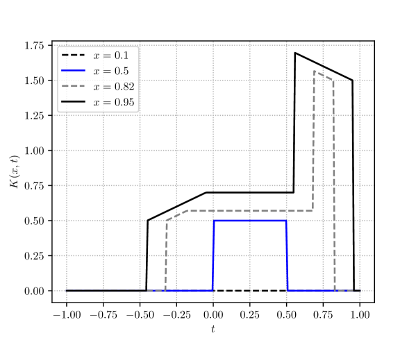
Figure 1: The graphs of $K_{\mathfrak{I}_{2}}^{0}(x,t)$, as a function of $t\in[-1,1]$, for some points $x\in(0,1)$ and $\mathfrak{I_{2}}=\{(0.25,1),(0.75,2)\}$.

For the general case we have the following representation for the kernel.

Proposition 13

The transmutation kernel $K_{\mathfrak{I}_{N}}^{0}(\rho,x)$ for the solution $e_{\mathfrak{I}_{N}}^{0}(\rho,x)$ of (15) is given by

$$K_{\mathfrak{I}_{N}}^{0}(x,t) =\sum_{k=0}^{N}\frac{\alpha_{k}H(x-x_{k})}{2}\chi_{[2x_{k}-x,x]}(t)$$

$$+\sum_{J\in\mathcal{J}_{N}}\frac{\alpha_{J}H(x-x_{j_{|J|}})}{2^{|J|}}\left(\left(\prod_{l=1}^{|J|-1}\right)^{\ast}\chi_{x_{j_{l+1}}-x_{j_{l}}}(t)\right)\ast\chi_{x-x_{j_{|J|}}}(t-x_{j_{1}})$$ (23)

Proof. In this case $\widetilde{e}_{0}(\rho,x)=e^{i\rho x}$, $\widehat{s}_{k}(\rho,x-x_{k})=\frac{\sin(\rho(x-x_{k}))}{\rho}$, hence $\widetilde{K}^{0}(x,t)\equiv 0$, $\widetilde{K}_{k}(x,t)=\frac{1}{2}\chi_{x-x_{k}}(t)$. Substituting these expressions into (22) and taking into account that $\chi_{x_{j_{|J|}}+x_{j_{1}}-x,x-(x_{j_{|J|}}-x_{j_{1}})}(t)=\chi_{x-x_{j_{|J|}}}(t-x_{j_{1}})$ we obtain (23)   

Let

$$\mathbf{T}_{\mathfrak{I}_{N}}^{h}u(x):=u(x)+\int_{-x}^{x}K_{\mathfrak{I}_{N}}^{h}(x,t)u(t)dt.$$ (24)

By Theorem 10, $\mathbf{T}_{\mathfrak{I}_{N}}^{f}\in\mathcal{B}\left(L_{2}(-b,b)\right)$ and

$$e_{\mathfrak{I}_{N}}^{h}(\rho,x)=\mathbf{T}_{\mathfrak{I}_{N}}^{h}\left[e^{i\rho x}\right].$$ (25)

4.2 Goursat conditions

Let us define the function

$$\sigma_{\mathfrak{I}_{N}}(x):=\sum_{k=1}^{N}\alpha_{k}H(x-x_{k}).$$ (26)

Hence $\sigma_{\mathfrak{I}_{N}}^{\prime}(x)=q_{\delta,\mathfrak{I}_{n}}(x)$ in the distributional sense ( $(\sigma_{\mathfrak{I}_{N}},\phi)_{C_{0}^{\infty}(0,b)}=-(q_{\delta,\mathfrak{I}_{N}},\phi^{\prime})_{C_{0}^{\infty}(0,b)}$ for all $\phi\in C_{0}^{\infty}(0,b)$). Note that in Examples 11 and 12 we have

$$K_{\mathfrak{J}_{N}}^{0}(x,x)=\frac{1}{2}\left(\int_{0}^{x}q(s)ds+\sigma_{\mathfrak{I}_{N}}(x)\right)\;\,\mbox{ and }\;\,K_{\mathfrak{I}_{N}}^{0}(x,-x)=0\;\,\mbox{ for }N=1,2.$$

More generally, the following statement is true.

Proposition 14

The integral transmutation kernel $K_{\mathfrak{I}_{N}}^{h}$ satisfies the following Goursat conditions for $x\in[0,b]$

$$K_{\mathfrak{J}_{N}}^{h}(x,x)=\frac{1}{2}\left(h+\int_{0}^{x}q(s)ds+\sigma_{\mathfrak{I}_{N}}(x)\right)\qquad\mbox{ and }\qquad K_{\mathfrak{I}_{N}}^{h}(x,-x)=\frac{h}{2}.$$ (27)

Proof. Fix $x\in[0,b]$ and take $\xi\in\{-x,x\}$. By formula (22) we can write

$$K_{\mathfrak{I}_{N}}^{h}(x,\xi)=\widetilde{K}^{h}(x,\xi)+\sum_{k=1}^{N}\alpha_{k}H(x-x_{k})\chi_{[2x_{k}-x,x]}(\xi)\widetilde{K}_{k}(x,\xi-x_{k})+F(x,\xi),$$

where

$$F(x,t)= \sum_{k=1}^{n}\alpha_{k}H(x-x_{k})\chi_{x_{k}}(t)\widetilde{K}^{h}(x_{k},t)\ast\chi_{x-x_{k}}(t)\widetilde{K}_{k}(x,t)$$

$$+\sum_{J\in\mathcal{J}_{N}}\alpha_{J}H(x-x_{j_{|J|}})\left(\prod_{l=1}^{|J|-1}\right)^{\ast}\left(\chi_{x_{j_{l+1}}-x_{j_{l}}}(t)\widetilde{K}_{j_{l}}(x_{j_{l+1}},t)\right)$$

$$\qquad\ast\Big{(}\chi_{x-(x_{j_{|J|}}-x_{j_{1}})}(t)\widetilde{K}_{j_{|J|}}(x,t-x_{j_{1}})+\chi_{x_{j_{1}}}(t)\widetilde{K}^{h}(x_{j_{1}},t)\ast\chi_{x-x_{j_{|J|}}}(t)\widetilde{K}_{j_{|J|}}(x,t)\Big{)}.$$

In the proof of Theorem 10 we obtain that $\operatorname{Supp}(F(x,t))\subset[-x,x]$. Since $\widetilde{K}^{h}(x_{j},t)$ and $\widetilde{K}_{k}(x_{j},t)$ are continuous with respect to $t$ in the intervals $[-x_{j},x_{j}]$ and $[x_{k}-x_{j},x_{j}-x_{k}]$ respectively for $j=1,\dots,N$, $k\leqslant j$, by Lemma 9 the function $F(x,t)$ is continuous for all $t\in\mathbb{R}$. Thus $F(x,\xi)=0$. For the case $\xi=x$, we have that $\widetilde{K}^{h}(x,x)=\frac{h}{2}+\frac{1}{2}\int_{0}^{x}q(s)ds$, $\chi_{[2x_{k}-x,x]}(x)=1$ and

$$\widetilde{K}_{k}(x,x-x_{k})=\frac{1}{2}\chi_{x-x_{k}}(x-x_{k})+\displaystyle\frac{1}{2}\int_{|x-x_{k}|}^{x-x_{k}}\widehat{H}_{k}(x-x_{k},s)ds=\frac{1}{2}$$

(we assume that $x\geqslant x_{k}$ in order to have $H(x-x_{k})=1$). Thus
$K_{\mathfrak{I}_{N}}^{h}(x,x)=\frac{1}{2}\left(h+\int_{0}^{x}q(s)ds+\sigma_{\mathfrak{I}_{N}}(x)\right)$. For the case $\xi=-x$, $\widetilde{K}^{h}(x,-x)=\frac{h}{2}$ and
$\chi_{[2x_{k}-x,x]}(-x)=0$. Hence $K_{\mathfrak{I}_{N}}^{h}(x,x)=\frac{h}{2}$.   

Remark 15

According to Proposition 14, $2K_{\mathfrak{I}_{N}}^{h}(x,x)$ is a (distributional) antiderivative of the potential $q(x)+q_{\delta,\mathfrak{I}_{N}}(x)$.

4.3 The transmuted Cosine and Sine solutions

Let $c_{\mathfrak{I}_{N}}^{h}(\rho,x)$ and $s_{\mathfrak{I}_{N}}(\rho,x)$ be the solutions of Eq. (1) satisfying the initial conditions

$$c_{\mathfrak{I}_{N}}^{h}(\rho,0)=1, (c_{\mathfrak{I}_{N}}^{h})^{\prime}(\rho,0)=h,$$ (28)

$$s_{\mathfrak{I}_{N}}(\rho,0)=0, s_{\mathfrak{I}_{N}}^{\prime}(\rho,0)=1.$$ (29)

Note that $c_{\mathfrak{I}_{N}}^{h}(\rho,x)=\frac{e_{\mathfrak{I}_{N}}^{h}(\rho,x)+e_{\mathfrak{I}_{N}}^{h}(-\rho,x)}{2}$ and $s_{\mathfrak{I}_{N}}(\rho,x)=\frac{e_{\mathfrak{I}_{N}}^{h}(\rho,x)-e_{\mathfrak{I}_{N}}^{h}(-\rho,x)}{2i\rho}$.

Remark 16

By Corollary 3, $c_{\mathfrak{I}_{N}}^{h}(\rho,\cdot),s_{\mathfrak{I}_{N}}(\rho,\cdot)\in AC[0,b]$ and both functions are solutions of Eq. (9) on $[0,x_{1}]$, hence their Wronskian is constant for $x\in[0,x_{1}]$ and

$$1 =W\left[c_{\mathfrak{I}_{N}}^{h}(\rho,x),s_{\mathfrak{I}_{N}}(\rho,x)\right](0)=W\left[c_{\mathfrak{I}_{N}}^{h}(\rho,x),s_{\mathfrak{I}_{N}}(\rho,x)\right](x_{1}-)=\begin{vmatrix}c_{\mathfrak{I}_{N}}^{h}(\rho,x_{1})&s_{\mathfrak{I}_{N}}(\rho,x_{1})\\ (c_{\mathfrak{I}_{N}}^{h})^{\prime}(\rho,x_{1}-)&s^{\prime}_{\mathfrak{I}_{N}}(\rho,x_{1}-)\end{vmatrix}$$

$$=\begin{vmatrix}c_{\mathfrak{I}_{N}}^{h}(\rho,x_{1})&s_{\mathfrak{I}_{N}}(\rho,x_{1})\\ (c_{\mathfrak{I}_{N}}^{h})^{\prime}(\rho,x_{1}+)-\alpha_{1}c_{\mathfrak{I}_{N}}^{h}(\rho,x_{1})&s^{\prime}_{\mathfrak{I}_{N}}(\rho,x_{1}+)-\alpha_{1}s_{\mathfrak{I}_{N}}(\rho,x_{1})\end{vmatrix}$$

$$=\begin{vmatrix}c_{\mathfrak{I}_{N}}^{h}(\rho,x_{1})&s_{\mathfrak{I}_{N}}(\rho,x_{1})\\ (c_{\mathfrak{I}_{N}}^{h})^{\prime}(\rho,x_{1}+)&s^{\prime}_{\mathfrak{I}_{N}}(\rho,x_{1}+)\end{vmatrix}=W\left[c_{\mathfrak{I}_{N}}^{h}(\rho,x),s_{\mathfrak{I}_{N}}(\rho,x)\right](x_{1}+)$$

(the equality in the second line is due to (2)). Since $c_{\mathfrak{I}_{N}}^{h}(\rho,x),s_{\mathfrak{I}_{N}}(\rho,x)$ are solutions of (9) on $[x_{1},x_{2}]$, then $W\left[C_{\mathfrak{I}_{N}}^{h}(\rho,x),s_{\mathfrak{I}_{N}}(\rho,x)\right]$ is constant for $x\in[x_{1},x_{2}]$. Thus,
$W\left[c_{\mathfrak{I}_{N}}^{h}(\rho,x),s_{\mathfrak{I}_{N}}(\rho,x)\right](x)=1$ for all $x\in[0,x_{2}]$. Continuing the process we obtain that the Wronskian equals one in the whole segment $[0,b]$. Thus, $c_{\mathfrak{I}_{N}}^{h}(\rho,x),s_{\mathfrak{I}_{N}}(\rho,x)$ are linearly independent. Finally, if $u$ is a solution of (1), by Remark 5, $u$ can be written as $u(x)=u(0)c_{\mathfrak{I}_{N}}^{h}(\rho,x)+u^{\prime}(0)s_{\mathfrak{I}_{N}}(\rho,x)$. In this way, $\left\{c_{\mathfrak{I}_{N}}^{h}(\rho,x),s_{\mathfrak{I}_{N}}(\rho,x)\right\}$ is a fundamental set of solutions for (1).

Similarly to the case of the regular Eq. (13) (see [39, Ch. 1]), from (21) we obtain the following representations.

Proposition 17

The solutions $c_{\mathfrak{I}_{N}}^{h}(\rho,x)$ and $s_{\mathfrak{I}_{N}}(\rho,x)$ admit the following integral representations

$$c_{\mathfrak{I}_{N}}^{h}(\rho,x) =\cos(\rho x)+\int_{0}^{x}G_{\mathfrak{I}_{N}}^{h}(x,t)\cos(\rho t)dt,$$ (30)

$$s_{\mathfrak{I}_{N}}(\rho,x) =\frac{\sin(\rho x)}{\rho}+\int_{0}^{x}S_{\mathfrak{I}_{N}}(x,t)\frac{\sin(\rho t)}{\rho}dt,$$ (31)

where

$$G_{\mathfrak{I}_{N}}^{h}(x,t) =K_{\mathfrak{I}_{N}}^{h}(x,t)+K_{\mathfrak{I}_{N}}^{h}(x,-t),$$ (32)

$$S_{\mathfrak{I}_{N}}(x,t) =K_{\mathfrak{I}_{N}}^{h}(x,t)-K_{\mathfrak{I}_{N}}^{h}(x,-t).$$ (33)

Remark 18

By Proposition 14, the cosine and sine integral transmutation kernels satisfy the conditions

$$G_{\mathfrak{I}_{N}}^{h}(x,x)=h+\frac{1}{2}\left(\int_{0}^{x}q(s)ds+\sigma_{\mathfrak{I}_{N}}(x)\right),$$ (34)

$$S_{\mathfrak{I}_{N}}(x,x)=\frac{1}{2}\left(\int_{0}^{x}q(s)ds+\sigma_{\mathfrak{I}_{N}}(x)\right)\quad\mbox{and }\;\;S_{\mathfrak{I}_{N}}(x,0)=0.$$ (35)

Introducing the cosine and sine transmutation operators

$$\mathbf{T}_{\mathfrak{I}_{N},h}^{C}u(x)=u(x)+\int_{0}^{x}G_{\mathfrak{I}_{N}}^{h}(x,t)u(t)dt,\quad\mathbf{T}_{\mathfrak{I}_{N}}^{S}u(x)=u(x)+\int_{0}^{x}S_{\mathfrak{I}_{N}}(x,t)u(t)dt$$ (36)

we obtain

$$c_{\mathfrak{I}_{N}}^{h}(\rho,x)=\mathbf{T}_{\mathfrak{I}_{N},h}^{C}\left[\cos(\rho x)\right],\quad s_{\mathfrak{I}_{N}}(\rho,x)=\mathbf{T}_{\mathfrak{I}_{N}}^{S}\left[\frac{\sin(\rho x)}{\rho}\right].$$ (37)

Remark 19

According to Remark 16, the space of solutions of (1) has dimension 2, and given $f,g\in\mathcal{D}_{2}\left(\mathbf{L}_{q,\mathfrak{I}_{N}}\right)$ solutions of (1), repeating the same procedure of Remark 16, $W[f,g]$ is constant in the whole segment $[0,b]$. The solutions $f,g$ are a fundamental set of solutions iff $W[f,g]\neq 0$.

5 The SPPS method and the mapping property

5.1 Spectral parameter powers series

As in the case of the regular Schrödinger equation [10, 31], we obtain a representation for the solutions of (1) as a power series in the spectral parameter (SPPS series). Assume that there exists a solution $f\in\mathcal{D}_{2}\left(\mathbf{L}_{q,\mathfrak{I}_{N}}\right)$ that does not vanish in the whole segment $[0,b]$.

Remark 20

Given $g\in L_{2}(0,b)$, a solution $u\in\mathcal{D}_{2}\left(\mathbf{L}_{q,\mathfrak{I}_{N}}\right)$ of the non-homogeneous Cauchy problem

$$\begin{cases}\mathbf{L}_{q,\mathfrak{I}_{N}}u(x)=g(x),\quad 0<x<b\\ u(0)=u_{0},\;u^{\prime}(0)=u_{1}\end{cases}$$ (38)

can be obtained by solving the regular equation $\mathbf{L}_{q}u(x)=g(x)$ a.e. $x\in(0,b)$ as follows. Consider the Polya factorization $\mathbf{L}_{q}u=-\frac{1}{f}Df^{2}D\frac{u}{f}$, where $D=\frac{d}{dx}$. A direct computation shows that $u$ given by

$$u(x)=-f(x)\int_{0}^{x}\frac{1}{f^{2}(t)}\int_{0}^{t}f(s)g(s)ds+\frac{u_{0}}{f(0)}f(x)+(f(0)u_{1}-f^{\prime}(0)u_{0})f(x)\int_{0}^{x}\frac{dt}{f^{2}(t)}$$ (39)

satisfies (38) (actually, $f(x)\int_{0}^{x}\frac{1}{f^{2}(t)}dt$ is the second linearly independent solution of $\mathbf{L}_{q}u=0$ obtained from $f$ by Abel’s formula). By Remark 4, $u\in\mathcal{D}_{2}\left(\mathbf{L}_{q,\mathfrak{J}_{N}}\right)$ and by Proposition 1 and Remark 5, formula (39) provides the unique solution of (38). Actually, if we denote $\mathcal{I}u(x):=\int_{0}^{x}u(t)dt$ and define $\mathbf{R}_{\mathfrak{I}_{N}}^{f}:=-f\mathcal{I}f^{2}\mathcal{I}$, then $\mathbf{R}_{\mathfrak{I}_{N}}^{f}\in\mathcal{B}\left(L_{2}(0,b)\right)$, $\mathbf{R}_{\mathfrak{I}_{N}}^{f}\left(L_{2}(0,b)\right)\subset\mathcal{D}_{2}\left(\mathbf{L}_{q,\mathfrak{I}_{N}}\right)$ and is a right-inverse for $\mathbf{L}_{q,\mathfrak{I}_{N}}$, i.e., $\mathbf{L}_{q,\mathfrak{I}_{N}}\mathbf{R}_{\mathfrak{I}_{N}}^{f}g=g$ for all $g\in L_{2}(0,b)$.

Following [31] we define the following recursive integrals: $\widetilde{X}^{(0)}\equiv X^{(0)}\equiv 1$, and for $k\in\mathbb{N}$

$$\widetilde{X}^{(k)}(x) :=k\int_{0}^{x}\widetilde{X}^{(k-1)}(s)\left(f^{2}(s)\right)^{(-1)^{k-1}}ds,$$ (40)

$$X^{(k)}(x) :=k\int_{0}^{x}X^{(k-1)}(s)\left(f^{2}(s)\right)^{(-1)^{k}}ds.$$ (41)

The functions $\{\varphi_{f}^{(k)}(x)\}_{k=0}^{\infty}$ defined by

$$\varphi_{f}^{(k)}(x):=\begin{cases}f(x)\widetilde{X}^{(k)}(x),\quad\mbox{if }k\mbox{ even},\\ f(x)X^{(k)}(x),\quad\mbox{if }k\mbox{ odd}.\end{cases}$$ (42)

for $k\in\mathbb{N}_{0}$, are called the formal powers associated to $f$. Additionally, we introduce the following auxiliary formal powers $\{\psi_{f}^{(k)}(x)\}_{k=0}^{\infty}$ given by

$$\psi_{f}^{(k)}(x):=\begin{cases}\frac{\widetilde{X}^{(k)}(x)}{f(x)},\quad\mbox{if }k\mbox{ odd},\\ \frac{X^{(k)}(x)}{f(x)},\quad\mbox{if }k\mbox{ even}.\end{cases}$$ (43)

Remark 21

For each $k\in\mathbb{N}_{0}$, $\varphi_{f}^{(k)}\in\mathcal{D}_{2}\left(\mathbf{L}_{q,\mathfrak{I}_{N}}\right)$. Indeed, direct computations show that the following relations hold for all $k\in\mathbb{N}_{0}$:

$$D\varphi_{f}^{(k)} =\frac{f^{\prime}}{f}\varphi_{f}^{(k)}+k\psi_{f}^{(k-1)}$$ (44)

$$D^{2}\varphi_{f}^{(k)} =\frac{f^{\prime\prime}}{f}\varphi_{f}^{(k)}+k(k-1)\varphi_{f}^{(k-2)}$$ (45)

Since $\varphi_{f}^{(k)},\psi_{f}^{(k)}\in C[0,b]$, using the procedure from Remark 4 and (44) we obtain $\varphi_{f}^{(k)}\in\mathcal{D}_{2}\left(\mathbf{L}_{q,\mathfrak{I}_{N}}\right)$.

Theorem 22 (SPPS method)

Suppose that $f\in\mathcal{D}_{2}\left(\mathbf{L}_{q,\mathfrak{I}_{N}}\right)$ is a solution of (1) that does not vanish in the whole segment $[0,b]$. Then the functions

$$u_{0}(\rho,x)=\sum_{k=0}^{\infty}\frac{(-1)^{k}\rho^{2k}\varphi_{f}^{(2k)}(x)}{(2k)!},\quad u_{1}(\rho,x)=\sum_{k=0}^{\infty}\frac{(-1)^{k}\rho^{2k}\varphi_{f}^{(2k+1)}(x)}{(2k+1)!}$$ (46)

belong to $\mathcal{D}_{2}\left(\mathbf{L}_{q,\mathfrak{I}_{N}}\right)$, and $\{u_{0}(\rho,x),u_{1}(\rho,x)\}$ is a fundamental set of solutions for (1) satisfying the initial conditions

$$u_{0}(\rho,0)=f(0), u^{\prime}_{0}(\rho,0)=f^{\prime}(0),$$ (47)

$$u_{1}(\rho,0)=0, u^{\prime}_{1}(\rho,0)=\frac{1}{f(0)},$$ (48)

The series in (46) converge absolutely and uniformly on $x\in[0,b]$, the series of the derivatives converge in $L_{2}(0,b)$ and the series of the second derivatives converge in $L_{2}(x_{j},x_{j+1})$, $j=0,\cdots,N$. With respect to $\rho$ the series converge absolutely and uniformly on any compact subset of the complex $\rho$-plane.

Proof. Since $f\in C[0,b]$, the following estimates for the recursive integrals $\{\widetilde{X}^{(k)}(x)\}_{k=0}^{\infty}$ and $\{X^{(k)}(x)\}_{k=0}^{\infty}$ are known:

$$|\widetilde{X}^{(n)}(x)|\leqslant M_{1}^{n}b^{n},\;|X^{(n)}(x)|\leqslant M_{1}^{n}b^{n}\quad\mbox{for all }x\in[0,b],$$ (49)

where $M_{1}=\|f^{2}\|_{C[0,b]}\cdot\left\|\frac{1}{f^{2}}\right\|_{C[0,b]}$ (see the proof of Theorem 1 of [31]). Thus, by the Weierstrass $M$-tests, the series in (46) converge absolutely and uniformly on $x\in[0,b]$, and for $\rho$ on any compact subset of the complex $\rho$-plane. We prove that $u_{0}(\rho,x)\in\mathcal{D}_{2}\left(\mathbf{L}_{q,\mathfrak{I}_{N}}\right)$ and is a solution of (1) (the proof for $u_{1}(\rho,x)$ is analogous). By Remark 21, the series of the derivatives of $u_{0}(\rho,x)$ is given by $\frac{f^{\prime}}{f}\sum_{k=0}^{\infty}\frac{(-1)^{k}\rho^{2k}\varphi_{f}^{(2k)}}{(2k)!}+\sum_{k=1}^{\infty}\frac{(-1)^{k}\rho^{2k}\psi_{f}^{(2k-1)}}{(2k-1)!}$. By (49), the series involving the formal powers $\varphi_{f}^{(k)}$ and $\psi_{f}^{(k)}$ converge absolutely and uniformly on $x\in[0,b]$. Hence, $\sum_{k=0}^{\infty}\frac{(-1)^{k}\rho^{k}D\varphi_{f}^{(2k)}(x)}{(2k)!}$ converges in $L_{2}(0,b)$. Due to [10, Prop. 3], $u_{0}(\rho,\cdot)\in AC[0,b]$ and $u_{0}^{\prime}(\rho,x)=\frac{f^{\prime}(x)}{f(x)}\sum_{k=0}^{\infty}\frac{(-1)^{k}\rho^{2k}\varphi_{f}^{(2k)}}{(2k)!}+\sum_{k=1}^{\infty}\frac{(-1)^{k}\rho^{2k}\psi_{f}^{(2k-1)}}{(2k-1)!}$ in $L_{2}(0,b)$. Since the series involving the formal powers defines continuous functions, then $u_{0}(\rho,x)$ satisfies the jump condition (2). Applying the same reasoning it is shown that $u_{0}^{\prime\prime}(\rho,x)=\sum_{k=0}^{\infty}\frac{(-1)^{k}\rho^{2k}D^{2}\varphi_{f}^{(2k)}}{(2k)!}$, the series converges in $L_{2}(x_{j},x_{j+1})$ and $u_{0}(\rho,\cdot)|_{(x_{j},x_{j+1})}\in H^{2}(x_{j},x_{j+1})$, $j=0,\dots,N$.

Since $\widetilde{X}^{(n)}(0)=0$ for $n\geqslant 1$, we have (47). Finally, by (45)

$$\mathbf{L}_{q}u_{0}(\rho,x) =\sum_{k=0}^{\infty}\frac{(-1)^{k}\rho^{2k}\mathbf{L}_{q}\varphi_{f}^{(2k)}(x)}{(2k)!}=\sum_{k=2}^{\infty}\frac{(-1)^{k+1}\rho^{2k}\varphi_{f}^{(2k-2)}(x)}{(2k-2)!}$$

$$=\rho^{2}\sum_{k=0}^{\infty}\frac{(-1)^{k}\rho^{2k}\varphi_{f}^{(2k)}(x)}{(2k)!}=\rho^{2}u(\rho,x),$$

this for a.e. $x\in(x_{j},x_{j+1})$, $j=0,\dots,N$.

Using (47) and (48) we obtain $W[u_{0}(\rho,x),u_{1}(\rho,x)](0)=1$. Since the Wronskian is constant (Remark 19), $\{u_{0}(\rho,x),u_{1}(\rho,x)\}$ is a fundamental set of solutions.   

5.2 Existence and construction of the non-vanishing solution

The existence of a non-vanishing solution is well known for the case of a regular Schrödinger equation with continuous potential (see [31, Remark 5] and [13, Cor. 2.3]). The following proof adapts the one presented in [21, Prop. 2.9] for the Dirac system.

Proposition 23 (Existence of non-vanishing solutions)

Let $\{u,v\}\in\mathcal{D}_{2}\left(\mathbf{L}_{q,\mathfrak{I}_{N}}\right)$ be a fundamental set of solutions for (1). Then there exist constants $c_{1},c_{2}\in\mathbb{C}$ such that the solution $f=c_{1}u+c_{2}v$ does not vanish in the whole segment $[0,b]$.

Proof. Let $\{u,v\}\in\mathcal{D}_{2}\left(\mathbf{L}_{q,\mathfrak{I}_{N}}\right)$ be a fundamental set of solutions for (1). Then $u$ and $v$ cannot have common zeros in $[0,b]$. Indeed, if $u(\xi)=v(\xi)=0$ for some $\xi\in[0,b]$, then $W[u,v](\xi+)=u(\xi)v^{\prime}(\xi+)-v(\xi)u^{\prime}(\xi+)=0$. Since $W[u,v]$ is constant in $[0,b]$, this contradicts that $\{u,v\}$ is a fundamental system.

This implies that in each interval $[x_{j},x_{j+1}]$, $j=0,\cdots,N$, the map $F_{j}:[x_{j},x_{j+1}]\rightarrow\mathbb{CP}^{1}$, $F_{j}(x):=\left[u|_{[x_{j},x_{j+1}]}(x):v|_{[x_{j},x_{j+1}]}(x)\right]$ (where $\mathbb{CP}^{1}$ is the complex projective line, i.e., the quotient of $\mathbb{C}^{2}\setminus\{(0,0)\}$ under the action of $\mathbb{C}^{*}$, and $[a:b]$ denotes the equivalent class of the pair $(a,b)$) is well defined and differentiable. In [13, Prop. 2.2] it was established that a differentiable function $f:I\rightarrow\mathbb{CP}^{1}$, where $I\subset\mathbb{R}$ is an interval, is never surjective, using that Sard’s theorem implies that $f(I)$ has measure zero.

Suppose that $(\alpha,\beta)\in\mathbb{C}^{2}\setminus\{(0,0)\}$ is such that $\alpha u(\xi)-\beta v(\xi)=0$ for some $\xi\in[0,b]$. Hence $\begin{vmatrix}u(\xi)&\beta\\ v(\xi)&\alpha\end{vmatrix}=0$, that is, $(u(\xi),v(\xi))$ and $(\alpha,\beta)$ are proportional. Since $\xi\in[x_{j},x_{j+1}]$ for some $j\in\{0,\cdots,N\}$, hence $[\alpha:-\beta]\in F_{j}\left([x_{j},x_{j+1}]\right)$.

Thus, the set $C:=\left\{[\alpha:\beta]\in\mathbb{CP}^{1}\,|\,\exists\xi\in[0,b]\,:\,\alpha u(\xi)+\beta v(\xi)=0\right\}$ is contained in
$\cup_{j=0}^{N}F_{j}\left([x_{j},x_{j+1}]\right)$, and then $C$ has measure zero. Hence we can obtain a pair of constants $(c_{1},c_{2})\in\mathbb{C}^{2}\setminus\{(0,0)\}$ with $[c_{1}:-c_{2}]\in\mathbb{CP}^{1}\setminus C$ and $f=c_{1}u+c_{2}v$ does not vanish in the whole segment $[0,b]$.   

Remark 24

If $q$ is real valued and $\alpha_{1},\cdots,\alpha_{N}\in\mathbb{R}\setminus\{0\}$, taking a real-valued fundamental system of solutions for the regular equation $\mathbf{L}_{q}y=0$ and using formula (12), we can obtain a real-valued fundamental set of solutions $\{u,v\}$ for $\mathbf{L}_{q,\mathfrak{I}_{N}}y=0$. In the proof of Proposition 23 we obtain that $u$ and $v$ have no common zeros. Hence $f=u+iv$ is a non vanishing solution.

For the complex case, we can choose randomly a pair of constants $(c_{1},c_{2})\in\mathbb{C}^{2}\setminus\{(0,0)\}$ and verify if the linear combination $c_{1}u+c_{2}v$ has no zero. If there is a zero, we repeat the process until we find the non vanishing solution. Since the set $C$ (from the proof of Proposition 23) has measure zero, is almost sure to find the coefficients $c_{1},c_{2}$ in the first few tries.

By Proposition 23, there exists a pair of constants $(c_{1},c_{2})\in\mathbb{C}^{2}\setminus\{(0,0)\}$ such that

$$y_{0}(x) =c_{1}+c_{2}x+\sum_{k=1}^{N}\alpha_{k}(c_{1}+c_{2}x_{k})H(x-x_{k})(x-x_{k})$$

$$\quad+\sum_{J\in\mathcal{J}_{N}}\alpha_{J}(c_{1}+c_{2}x_{j_{1}})H(x-x_{j_{|J|}})\left(\prod_{l=1}^{|J|-1}(x_{j_{l+1}}-x_{j_{1}})\right)(x-x_{j_{|J|}})$$ (50)

is a non-vanishing solution of (1) for $\rho=0$ (if $\alpha_{1},\dots,\alpha_{k}\in(0,\infty)$, it is enough with take $c_{1}=1$, $c_{2}=0$). Below we give a procedure based on the SPPS method ([10, 31]) to obtain the non-vanishing solution $f$ from $y_{0}$.

Theorem 25

Define the recursive integrals $\{Y^{(k)}\}_{k=0}^{\infty}$ and $\{\tilde{Y}^{(k)}\}_{k=0}^{\infty}$ as follows: $Y^{(0)}\equiv\tilde{Y}^{(0)}\equiv 1$, and for $k\geqslant 1$

$$Y^{(k)}(x) =\begin{cases}\int_{0}^{x}Y^{(k)}(s)q(s)y_{0}^{2}(s)ds,&\mbox{ if }k\mbox{ is even},\\ \int_{0}^{x}\frac{Y^{(k)}(s)}{y_{0}^{2}(s)}ds,&\mbox{ if }k\mbox{ is odd},\end{cases}$$ (51)

$$\tilde{Y}^{(k)}(x) =\begin{cases}\int_{0}^{x}\tilde{Y}^{(k)}(s)q(s)y_{0}^{2}(s)ds,&\mbox{ if }k\mbox{ is odd},\\ \int_{0}^{x}\frac{\tilde{Y}^{(k)}(s)}{y_{0}^{2}(s)}ds,&\mbox{ if }k\mbox{ is even}.\end{cases}$$ (52)

Define

$$f_{0}(x)=y_{0}(x)\sum_{k=0}^{\infty}\tilde{Y}^{(2k)}(x),\qquad f_{1}(x)=y_{0}(x)\sum_{k=0}^{\infty}Y^{(2k+1)}(x).$$ (53)

Then $\{f_{0},f_{1}\}\subset\mathcal{D}_{2}\left(\mathbf{L}_{q,\mathfrak{I}_{N}}\right)$ is a fundamental set of solution for $\mathbf{L}_{q,\mathfrak{I}_{N}}u=0$ satisfying the initial conditions $f_{0}(0)=c_{1}$, $f^{\prime}_{0}(0)=c_{2}$, $f_{1}(0)=0$, $f^{\prime}_{1}(0)=1$. Both series converge uniformly and absolutely on $x\in[0,b]$. The series of the derivatives converge in $L_{2}(0,b)$, and on each interval $[x_{j},x_{j+1}]$, $j=0,\dots,N$, the series of the second derivatives converge in $L_{2}(x_{j},x_{j+1})$. Hence there exist constants $C_{1},C_{2}\in\mathbb{C}$ such that $f=C_{1}f_{0}+C_{2}f_{1}$ is a non-vanishing solution of $\mathbf{L}_{q,\mathfrak{I}_{N}}u=0$ in $[0,b]$.

Proof. Using the estimates

$$|\tilde{Y}^{(2k-j)}(x)|\leqslant\frac{M_{1}^{(n-j)}M_{2}^{n}}{(n-j)!n!},\quad|Y^{(2k-j)}(x)|\leqslant\frac{M_{1}^{n}M_{2}^{(n-j)}}{n!(n-j)!},\quad x\in[0,b],\;j=0,1,\;k\in\mathbb{N},$$

where $M_{1}=\left\|\frac{1}{y_{0}^{2}}\right\|_{L_{1}(0,b)}$ and $M_{2}=\|qy_{0}^{2}\|_{L_{1}(0,b)}$, from [10, Prop. 5], the series in (53) converge absolutely and uniformly on $[0,b]$. The proof of the convergence of the derivatives and that $\{f_{0},f_{1}\}\in\mathcal{D}_{2}\left(\mathbf{L}_{q,\mathfrak{I}_{N}}\right)$ is a fundamental set of solutions is analogous to that of Theorem 22 (see also [31, Th. 1]) and [10, Th. 7] for the proof in the regular case).   

5.3 The mapping property

Take a non vanishing solution $f\in\mathcal{D}_{2}\left(\mathbf{L}_{q,\mathfrak{I}_{N}}\right)$ normalized at zero, i.e., $f(0)=1$, and set $h=f^{\prime}(0)$. Then the corresponding transmutation operator and kernel $\mathbf{T}^{h}_{\mathfrak{I}_{N}}$ and $K_{\mathfrak{I}_{N}}^{h}(x,t)$ will be denoted by $\mathbf{T}^{f}_{\mathfrak{I}_{N}}$ and $K_{\mathfrak{I}_{N}}^{f}(x,t)$ and called the canonical transmutation operator and kernel associated to $f$, respectively (same notations are used for the cosine and sine transmutations).

Theorem 26

The canonical transmutation operator $\mathbf{T}^{f}_{\mathfrak{I}_{N}}$ satisfies the following relations

$$\mathbf{T}_{\mathfrak{I}_{N}}^{f}\left[x^{k}\right]=\varphi_{f}^{(k)}(x)\qquad\forall k\in\mathbb{N}_{0}.$$ (54)

The canonical cosine and sine transmutation operators satisfy the relations

$$\mathbf{T}_{\mathfrak{I}_{N},f}^{C}\left[x^{2k}\right] =\varphi_{f}^{(2k)}(x)\qquad\forall k\in\mathbb{N}_{0}.$$ (55)

$$\mathbf{T}_{\mathfrak{I}_{N}}^{S}\left[x^{2k+1}\right] =\varphi_{f}^{(2k+1)}(x)\qquad\forall k\in\mathbb{N}_{0}.$$ (56)

Proof. Consider the solution $e_{\mathfrak{I}_{N}}^{h}(\rho,x)$ with $h=f^{\prime}(0)$. By the conditions (47) and (48), solution $e_{\mathfrak{I}_{N}}^{h}(\rho,x)$ can be written in the form

$$e_{\mathfrak{I}_{N}}^{h}(\rho,x) =u_{0}(\rho,x)+i\rho u_{1}(\rho,x)$$

$$=\sum_{k=0}^{\infty}\frac{(-1)^{k}\rho^{2k}\varphi_{f}^{(2k)}(x)}{(2k)!}+\sum_{k=0}^{\infty}\frac{i(-1)^{k}\rho^{2k+1}\varphi_{f}^{(2k+1)}(x)}{(2k+1)!}$$

$$=\sum_{k=0}^{\infty}\frac{(i\rho)^{2k}\varphi_{f}^{(2k)}(x)}{(2k)!}+\sum_{k=0}^{\infty}\frac{(i\rho)^{2k+1}\varphi_{f}^{(2k+1)}(x)}{(2k+1)!}$$

$$=\sum_{k=0}^{\infty}\frac{(i\rho)^{k}\varphi_{f}^{(k)}(x)}{k!}$$ (57)

(The rearrangement of the series is due to absolute and uniform convergence, Theorem 22). On the other hand

$$e_{\mathfrak{I}_{N}}^{h}(\rho,x)=\mathbf{T}_{\mathfrak{I}_{N}}^{f}\left[e^{i\rho x}\right]=\mathbf{T}_{\mathfrak{I}_{N}}^{f}\left[\sum_{k=0}^{\infty}\frac{(i\rho)^{k}x^{k}}{k!}\right]$$

Note that $\displaystyle\int_{-x}^{x}K_{\mathfrak{I}_{N}}^{f}(x,t)\left(\sum_{k=0}^{\infty}\frac{(i\rho)^{k}t^{k}}{k!}\right)dt=\sum_{k=0}^{\infty}\frac{(i\rho)^{k}}{k!}\int_{-x}^{x}K_{\mathfrak{I}_{N}}^{f}(x,t)t^{k}dt$, due to the uniform convergence of the exponential series in the variable $t\in[-x,x]$. Thus,

$$e_{\mathfrak{I}_{N}}^{h}(\rho,x)=\sum_{k=0}^{\infty}\frac{(i\rho)^{k}\mathbf{T}_{\mathfrak{I}_{N}}^{f}\left[x^{k}\right]}{k!}.$$ (58)

Comparing (58) and (57) as Taylor series in the complex variable $\rho$ we obtain (54). Relations (55) and (56) follows from (54), (32), (33) and the fact that $G_{\mathfrak{I}_{N}}^{f}(x,t)$ and $S_{\mathfrak{I}_{N}}(x,t)$ are even and odd in the variable $t$, respectively.   

Remark 27

The formal powers $\{\varphi_{f}^{(k)}(x)\}_{k=0}^{\infty}$ satisfy the asymptotic relation
$\varphi_{f}^{(k)}(x)=x^{k}(1+o(1))$, $x\rightarrow 0^{+}$, $\forall k\in\mathbb{N}$.

Indeed, by Theorem 26 and the Cauchy-Bunyakovsky-Schwarz inequality we have

$$|\varphi_{f}^{(k)}(x)-x^{k}| =\left|\int_{-x}^{x}K_{\mathfrak{I}_{N}}^{f}(x,t)t^{k}dt\right|\leqslant\left(\int_{-x}^{x}\left|K_{\mathfrak{I}_{N}}^{f}(x,t)\right|^{2}dt\right)^{\frac{1}{2}}\left(\int_{-x}^{x}|t|^{2k}dt\right)^{\frac{1}{2}}$$

$$\leqslant\sqrt{2b}\left\|K_{\mathfrak{I}_{N}^{f}}\right\|_{L_{\infty}(\Omega)}\sqrt{\frac{2}{2k+1}}x^{k+\frac{1}{2}}$$

(because $K_{\mathfrak{I}_{N}}^{f}\in L_{\infty}(\Omega)$ by Theorem 10). Hence

$$\left|\frac{\varphi_{f}^{(k)}(x)}{x^{k}}-1\right|\leqslant\sqrt{2b}\left\|K_{\mathfrak{I}_{N}^{f}}\right\|_{L_{\infty}(\Omega)}\sqrt{\frac{2}{2k+}}x^{\frac{1}{2}}\rightarrow 0,\qquad x\rightarrow 0^{+}.$$

Remark 28

Denote $\mathcal{P}(\mathbb{R})=\mbox{Span}\{x^{k}\}_{k=0}^{\infty}$. According to Remark 21 and Proposition 1 we have that $\mathbf{T}_{\mathfrak{I}_{N}}^{f}\left(\mathcal{P}(\mathbb{R})\right)=\mbox{Span}\left\{\varphi_{f}^{(k)}(x)\right\}_{k=0}^{\infty}$, and by (45) we have the relation

$$\mathbf{L}_{q,\mathfrak{I}_{N}}\mathbf{T}_{\mathfrak{I}_{N}}^{f}p=-\mathbf{T}_{\mathfrak{I}_{N}}^{f}D^{2}p\qquad\forall p\in\mathcal{P}(\mathbb{R}).$$ (59)

According to [14], $\mathbf{T}_{q,\mathfrak{I}_{N}}^{f}$ is a transmutation operator for the pair $\mathbf{L}_{q,\mathfrak{I}_{N}}$, $-D^{2}$ in the subspace $\mathcal{P}(\mathbb{R})$, and $\{\varphi_{f}^{(k)}(x)\}_{k=0}^{\infty}$ is an $\mathbf{L}_{q,\mathfrak{I}_{N}}$-basis. Since $\varphi_{f}^{(K)}(0)=D\varphi_{f}^{(k)}(0)=0$ for $k\geqslant 2$, $\{\varphi_{f}^{(k)}(x)\}_{k=0}^{\infty}$ is called a standard $\mathbf{L}_{q,\mathfrak{J}_{N}}$-basis, and $\mathbf{T}_{\mathfrak{I}_{N}}^{f}$ a standard transmutation operator. By Remark 20 we can recover $\varphi_{f}^{(k)}$ for $k\geqslant 2$ from $\varphi_{f}^{(0)}$ and $\varphi_{f}^{(0)}$ by the formula

$$\varphi_{f}^{(k)}(x)=-k(k-1)\mathbf{R}_{\mathfrak{I}_{N}}^{f}\varphi_{f}^{(k)}(x)=k(k-1)f(x)\int_{0}^{x}\frac{1}{f^{2}(t)}\int_{0}^{t}f(s)\varphi_{f}^{(k-2)}(s)ds$$ (60)

(compare this formula with [14, Formula (8), Remark 9]).

The following result adapts Theorem 10 from [14], proved for the case of an $L_{1}$-regular potential.

Theorem 29

The operator $\mathbf{T}_{\mathfrak{I}_{N}}^{f}$ is a transmutation operator for the pair $\mathbf{L}_{q,\mathfrak{I}_{N}}$, $-D^{2}$ in $H^{2}(-b,b)$, that is, $\mathbf{T}_{\mathfrak{I}_{N}}^{f}\left(H^{2}(-b,b)\right)\subset\mathcal{D}_{2}\left(\mathbf{L}_{q,\mathfrak{I}_{N}}\right)$ and

$$\mathbf{L}_{q,\mathfrak{I}_{N}}\mathbf{T}_{\mathfrak{I}_{N}}u=-\mathbf{T}_{\mathfrak{I}_{N}}D^{2}u\qquad\forall u\in H^{2}(-b,b)$$ (61)

Proof. We show that

$$\mathbf{T}_{\mathfrak{I}_{N}}u(x)=u(0)\varphi_{f}^{(0)}(x)+u^{\prime}(0)\varphi_{f}^{(1)}(x)-\mathbf{R}_{\mathfrak{I}_{N}}^{f}\mathbf{T}_{\mathfrak{I}_{N}}^{f}u^{\prime\prime 2}(-b,b).$$ (62)

Let us first see that (62) is valid for $p\in\mathcal{P}(\mathbb{R})$. Indeed, set $p(x)=\sum_{k=0}^{M}c_{k}x^{k}$. By the linearity of $\mathbf{T}_{\mathfrak{I}_{N}}^{f}$, Theorem 26 and (60) we have

$$\mathbf{T}_{\mathfrak{I}_{N}}^{f}p(x) =c_{0}\varphi_{f}^{(0)}+c_{1}\varphi_{f}^{(1)}(x)+\sum_{k=2}^{M}c_{k}\varphi_{f}^{(k)}(x)$$

$$=p(0)\varphi_{f}^{(0)}+p^{\prime}(0)\varphi_{f}^{(1)}(x)-\sum_{k=2}^{M}c_{k}k(k-1)\mathbf{R}_{\mathfrak{I}_{N}}^{f}\varphi_{f}^{(k-2)}(x)$$

$$=p(0)\varphi_{f}^{(0)}+p^{\prime}(0)\varphi_{f}^{(1)}(x)-\sum_{k=2}^{M}c_{k}k(k-1)\mathbf{R}_{\mathfrak{I}_{N}}^{f}\mathbf{T}_{\mathfrak{I}_{N}}^{f}\left[x^{k-2}\right]$$

$$=p(0)\varphi_{f}^{(0)}+p^{\prime}(0)\varphi_{f}^{(1)}(x)-\mathbf{R}_{\mathfrak{I}_{N}}^{f}\mathbf{T}_{\mathfrak{I}_{N}}^{f}p^{\prime\prime}(x)$$

This establishes (62) for $p\in\mathcal{P}(\mathbb{R})$. Take $u\in H^{2}(-b,b)$ arbitrary. There exists a sequence $\{p_{n}\}\subset\mathcal{P}(\mathbb{R})$ such that $p_{n}^{(j)}\overset{[-b,b]}{\rightrightarrows}u^{(j)}$, $j=0,1$, and $p^{\prime\prime}_{n}\rightarrow u$ in $L_{2}(-b,b)$, when $n\rightarrow\infty$ (see [14, Prop. 4]). Since $\mathbf{R}_{\mathfrak{I}_{N}}^{f}\mathbf{T}_{\mathfrak{I}_{N}}^{f}\in\mathcal{B}\left(L_{2}(-b,b),L_{2}(0,b)\right)$ we have

$$\mathbf{T}_{\mathfrak{I}_{N}}^{f}u(x) =\lim_{n\rightarrow\infty}\mathbf{T}_{\mathfrak{I}_{N}}^{f}p_{n}(x)=\lim_{n\rightarrow\infty}\left[p_{n}(0)\varphi_{f}^{(0)}+p^{\prime}_{n}(0)\varphi_{f}^{(1)}(x)-\mathbf{R}_{\mathfrak{I}_{N}}^{f}\mathbf{T}_{\mathfrak{I}_{N}}^{f}p^{\prime\prime}_{n}(x)\right]$$

$$=u(0)\varphi_{f}^{(0)}(x)+u^{\prime}(0)\varphi_{f}^{(1)}(x)-\mathbf{R}_{\mathfrak{I}_{N}}^{f}\mathbf{T}_{\mathfrak{I}_{N}}^{f}u^{\prime\prime}(x)$$

and we obtain (62). Hence, by Remark 20, $\mathbf{T}_{\mathfrak{I}_{N}}^{f}\left(H^{2}(-b,b)\right)\subset\mathcal{D}_{2}\left(\mathbf{L}_{q,\mathfrak{I}_{N}}\right)$, and since $\mathbf{L}_{q,\mathfrak{I}_{N}}\varphi_{f}^{(k)}=0$ for $k=0,1$, applying $\mathbf{L}_{q,\mathfrak{I}_{N}}$ in both sides of (62) we have (61).   

6 Fourier-Legendre and Neumann series of Bessel functions expansions

6.1 Fourier-Legendre series expansion of the transmutation kernel

Fix $x\in(0,b]$. Theorem 10 establishes that $K_{\mathfrak{I}_{N}}^{h}(x,\cdot)\in L_{2}(-x,x)$, then $K_{\mathfrak{I}_{N}}^{h}(x,t)$ admits a Fourier series in terms of an orthogonal basis of $L_{2}(-x,x)$. Following [30], we choose the orthogonal basis of $L_{2}(-1,1)$ given by the Legendre polynomials $\{P_{n}(z)\}_{n=0}^{\infty}$. Thus,

$$K_{\mathfrak{I}_{N}}^{h}(x,t)=\sum_{n=0}^{\infty}\frac{a_{n}(x)}{x}P_{n}\left(\frac{t}{x}\right)$$ (63)

where

$$a_{n}(x)=\left(n+\frac{1}{2}\right)\int_{-x}^{x}K_{\mathfrak{I}_{N}}^{h}(x,t)P_{n}\left(\frac{t}{x}\right)dt\qquad\forall n\in\mathbb{N}_{0}.$$ (64)

The series (63) converges with respect to $t$ in the norm of $L_{2}(-x,x)$. Formula (64) is obtained multiplying (63) by $P_{n}\left(\frac{t}{x}\right)$, using the general Parseval’s identity [2, pp. 16] and taking into account that $\|P_{n}\|_{L_{2}(-1,1)}^{2}=\frac{2}{2n+1}$, $n\in\mathbb{N}_{0}$.

Example 30

Consider the kernel $K_{\mathfrak{I}_{1}}^{0}(x,t)=\frac{\alpha_{1}}{2}H(x-x_{1})\chi_{[2x_{1}-x,x]}$ from Example 11. In this case, the Fourier-Legendre coefficients has the form

$$a_{n}(x)=\frac{\alpha_{1}}{2}\left(n+\frac{1}{2}\right)H(x-x_{1})\int_{2x_{1}-x}^{x}P_{n}(t)dt=\frac{\alpha_{1}}{2}\left(n+\frac{1}{2}\right)xH(x-x_{1})\int_{2\frac{x_{1}}{x}-1}^{1}P_{n}(t)dt.$$

From this we obtain $a_{0}(x)=\frac{\alpha_{1}}{2}H(x-x_{1})(x-x_{1})$. Using formula $P_{n}(t)=\frac{1}{2n+1}\frac{d}{dt}\left(P_{n+1}(t)-P_{n-1}(t)\right)$ for $n\in\mathbb{N}$, and that $P_{n}(1)=0$ for all $n\in\mathbb{N}$, we have

$$a_{n}(x)=\frac{\alpha_{1}}{4}xH(x-x_{1})\left[P_{n-1}\left(\frac{2x_{1}}{x}-1\right)-P_{n+1}\left(\frac{2x_{1}}{x}-1\right)\right]$$

Remark 31

From (64) we obtain that the first coefficient $a_{0}(x)$ is given by

$$a_{0}(x) =\frac{1}{2}\int_{-x}^{x}K_{\mathfrak{I}_{N}}^{h}(x,t)P_{0}\left(\frac{t}{x}\right)dt=\frac{1}{2}\int_{-x}^{x}K_{\mathfrak{I}_{N}}^{h}(x,t)dt$$

$$=\frac{1}{2}\mathbf{T}_{\mathfrak{I}_{N}}^{h}[1]-\frac{1}{2}=\frac{1}{2}(e_{\mathfrak{I}_{N}}^{h}(0,x)-1).$$

Thus, we obtain the relations

$$a_{0}(x)=\frac{1}{2}(e_{\mathfrak{I}_{N}}^{h}(0,x)-1),\qquad e_{\mathfrak{I}_{N}}^{h}(0,x)=2a_{n}(x)+1.$$ (65)

For the kernels $G_{\mathfrak{I}_{N}}^{h}(x,t)$ and $S_{\mathfrak{I}_{N}}(x,t)$ we obtain the series representations in terms of the even and odd Legendre polynomials, respectively,

$$G_{\mathfrak{I}_{N}}^{h}(x,t) =\sum_{n=0}^{\infty}\frac{g_{n}(x)}{x}P_{2n}\left(\frac{t}{x}\right),$$ (66)

$$S_{\mathfrak{I}_{N}}(x,t) =\sum_{n=0}^{\infty}\frac{s_{n}(x)}{x}P_{2n+1}\left(\frac{t}{x}\right),$$ (67)

where the coefficients are given by

$$g_{n}(x) =2a_{2n}(x)=(4n+1)\int_{0}^{x}G_{\mathfrak{I}_{N}}^{h}(x,t)P_{2n}\left(\frac{t}{x}\right)dt,$$ (68)

$$s_{n}(x) =2a_{2n+1}(4n+3)\int_{0}^{x}S_{\mathfrak{I}_{N}}(x,t)P_{2n+1}\left(\frac{t}{x}\right)dt.$$ (69)

The proof of these facts is analogous to that in the case of Eq. (9), see [30] or [29, Ch. 9].

Remark 32

Since $g_{0}(x)=2a_{0}(x)$, then $g_{0}(x)=e_{\mathfrak{I}_{N}}^{h}(0,x)-1$. Since $e_{\mathfrak{I}_{N}}^{h}(0,x)$ is the solution of (1) with $\rho=0$ satisfying $e_{\mathfrak{I}_{N}}^{h}(0,0)=1$, $(e_{\mathfrak{I}_{N}}^{h})^{\prime}(0,0)=h$, hence by Remark 5, $e_{\mathfrak{I}_{N}}^{h}(0,x)=c_{\mathfrak{I}_{N}}^{h}(0,x)$ and

$$g_{0}(x)=c_{\mathfrak{I}_{N}}^{h}(0,x)-1.$$ (70)

On the other hand, for the coefficient $s_{0}(x)$ we have the relation

$$s_{0}(x)=3\int_{0}^{x}H_{\mathfrak{I}_{N}}(x,t)P_{1}\left(\frac{t}{x}\right)dt=\frac{3}{x}\int_{0}^{x}H_{\mathfrak{I}_{N}}(x,t)tdt.$$

Since $\frac{\sin(\rho x)}{\rho}\big{|}_{x=0}=x$, from (31) we have

$$s_{0}(x)=3\left(\frac{s_{\mathfrak{I}_{N}}(0,x)}{x}-1\right).$$ (71)

For every $n\in\mathbb{N}_{0}$ we write the Legendre polynomial $P_{n}(z)$ in the form $P_{n}(z)=\sum_{k=0}^{n}l_{k,n}z^{k}$. Note that if $n$ is even, $l_{k,n}=0$ for odd $k$, and $P_{2n}(z)=\sum_{k=0}^{n}\tilde{l}_{k,n}z^{2k}$ with $\tilde{l}_{k,n}=l_{2k,2n}$. Similarly $P_{2n+1}(z)=\sum_{k=0}^{n}\hat{l}_{k,n}z^{2k+1}$ with $\hat{l}_{k,n}=l_{2k+1,2n+1}$. With this notation we write an explicit formula for the coefficients (64) of the canonical transmutation kernel $K_{\mathfrak{J}_{N}}^{f}(x,t)$.

Proposition 33

The coefficients $\{a_{n}(x)\}_{n=0}^{\infty}$ of the Fourier-Legendre expansion (63) of the canonical transmutation kernel $K_{\mathfrak{I}_{N}}^{f}(x,t)$ are given by

$$a_{n}(x)=\left(n+\frac{1}{2}\right)\left(\sum_{k=0}^{n}l_{k,n}\frac{\varphi_{f}^{(k)}(x)}{x^{k}}-1\right).$$ (72)

The coefficients of the canonical cosine and sine kernels satisfy the following relations for all $n\in\mathbb{N}_{0}$

$$g_{n}(x) =(4n+1)\left(\sum_{k=0}^{n}\tilde{l}_{k,n}\frac{\varphi_{f}^{(2k)}(x)}{x^{2k}}-1\right),$$ (73)

$$s_{n}(x) =(4n+3)\left(\sum_{k=0}^{n}\hat{l}_{k,n}\frac{\varphi_{f}^{(2k+1)}(x)}{x^{2k+1}}-1\right),$$ (74)

Proof. From (64) we have

$$a_{n}(x) =\left(n+\frac{1}{2}\right)\int_{-x}^{x}K_{\mathfrak{I}_{N}}^{f}(x,t)\left(\sum_{k=0}^{n}l_{k,n}\left(\frac{t}{x}\right)^{k}\right)dt$$

$$=\left(n+\frac{1}{2}\right)\sum_{k=0}^{n}\frac{l_{k,n}}{x^{k}}\int_{0}^{x}K_{\mathfrak{I}_{N}}^{f}(x,t)t^{k}dt$$

$$=\left(n+\frac{1}{2}\right)\sum_{k=0}^{n}\frac{l_{k,n}}{x^{k}}\left(\mathbf{T}_{\mathfrak{I}_{N}}^{f}\left[x^{k}\right]-x^{k}\right).$$

Hence (72) follows from Theorem 26 and that $P_{n}(z)=1$. Since $g_{n}(x)=2a_{2n}(x)$, $s_{n}(x)=2a_{2n+1}(x)$, $l_{2k+1,2n}=0$, $l_{2k,2n+1}=0$ and $l_{2k,2n}=\tilde{l}_{k,n}$,$l_{2k+1,2n+1}=\hat{l}_{k,n}$, we obtain (73) and (74).   

Remark 34

By Remark 27, formula (72) is well defined at $x=0$. Note that $x^{n}a_{n}(x)$ belongs to $\mathcal{D}_{2}\left(\mathbf{L}_{q,\mathfrak{I}_{N}}\right)$ for all $n\in\mathbb{N}_{0}$.

6.2 Representation of the solutions as Neumann series of Bessel functions

Similarly to the case of the regular Eq. (13) [30], we obtain a representation for the solutions in terms of Neumann series of Bessel functions (NSBF). For $M\in\mathbb{N}$ we define

$$K_{\mathfrak{I}_{N},M}^{h}(x,t):=\sum_{n=0}^{M}\frac{a_{n}(x)}{x}P_{n}\left(\frac{t}{x}\right),$$

that is, the $M$-partial sum of (63).

Theorem 35

The solutions $c_{\mathfrak{I}_{N}}^{h}(\rho,x)$ and $s_{\mathfrak{I}_{N}}(\rho,x)$ admit the following NSBF representations

$$c_{\mathfrak{I}_{N}}^{h}(\rho,x)=\cos(\rho x)+\sum_{n=0}^{\infty}(-1)^{n}g_{n}(x)j_{2n}(\rho x),$$ (75)

$$s_{\mathfrak{I}_{N}}(\rho,x)=\frac{\sin(\rho x)}{\rho}+\frac{1}{\rho}\sum_{n=0}^{\infty}(-1)^{n}s_{n}(x)j_{2n+1}(\rho x),$$ (76)

where $j_{\nu}$ stands for the spherical Bessel function $j_{\nu}(z)=\sqrt{\frac{\pi}{2z}}J_{\nu+\frac{1}{2}}(z)$ (and $J_{\nu}$ stands for the Bessel function of order $\nu$). The series converge pointwise with respect to $x$ in $(0,b]$ and uniformly with respect to $\rho$ on any compact subset of the complex $\rho$-plane. Moreover, for $M\in\mathbb{N}$ the functions

$$c_{\mathfrak{I}_{N},M}^{h}(\rho,x)=\cos(\rho x)+\sum_{n=0}^{M}(-1)^{n}g_{n}(x)j_{2n}(\rho x),$$ (77)

$$s_{\mathfrak{I}_{N},M}(\rho,x)=\frac{\sin(\rho x)}{\rho}+\frac{1}{\rho}\sum_{n=0}^{M}(-1)^{n}s_{n}(x)j_{2n+1}(\rho x),$$ (78)

obey the estimates

$$|c_{\mathfrak{I}_{N}}^{h}(\rho,x)-c_{\mathfrak{I}_{N},M}^{h}(\rho,x)| \leqslant 2\epsilon_{2M}(x)\sqrt{\frac{\sinh(2bC)}{C}},$$ (79)

$$|\rho s_{\mathfrak{I}_{N}}(\rho,x)-\rho s_{\mathfrak{I}_{N},M}(\rho,x)| \leqslant 2\epsilon_{2M+1}(x)\sqrt{\frac{\sinh(2bC)}{C}},$$ (80)

for any $\rho\in\mathbb{C}$ belonging to the strip $|\operatorname{Im}\rho|\leqslant C$, $C>0$, and where
$\epsilon_{M}(x)=\|K_{\mathfrak{I}_{N}}^{h}(x,\cdot)-K_{\mathfrak{I}_{N},2M}^{h}(x,\cdot)\|_{L_{2}(-x,x)}$.

Proof. We show the results for the solution $c_{\mathfrak{I}_{N}}^{h}(\rho,x)$ (the proof for $s_{\mathfrak{I}_{N}}(\rho,x)$ is similar). Substitution of the Fourier-Legendre series (66) in (30) leads us to

$$c_{\mathfrak{I}_{N}}^{h}(\rho,x) =\cos(\rho x)+\int_{0}^{x}\left(\sum_{n=0}^{\infty}\frac{g_{n}(x)}{x}P_{2n}\left(\frac{t}{x}\right)\right)\cos(\rho t)dt$$

$$=\cos(\rho x)+\sum_{n=0}^{\infty}\frac{g_{n}(x)}{x}\int_{0}^{x}P_{2n}\left(\frac{t}{x}\right)\cos(\rho t)dt$$

(the exchange of the integral with the summation is due to the fact that the integral is nothing but the inner product of the series with the function $\overline{\cos(\rho t)}$ and the series converges in $L_{2}(0,x)$). Using formula 2.17.7 in [40, pp. 433]

$$\int_{0}^{a}\left\{\begin{matrix}P_{2n+1}\left(\frac{y}{a}\right)\cdot\sin(by)\\ P_{2n}\left(\frac{y}{a}\right)\cdot\cos(by)\\ \end{matrix}\right\}dy=(-1)^{n}\sqrt{\frac{\pi a}{2b}}J_{2n+\delta+\frac{1}{2}}(ab),\quad\delta=\left\{\begin{matrix}1\\ 0\end{matrix}\right\},\;a>0,$$

we obtain the representation (75). Take $C>0$ and $\rho\in\mathbb{C}$ with $|\operatorname{Im}\rho|\leqslant C$. For $M\in\mathbb{N}$ define $G_{\mathfrak{I}_{N},M}^{h}(x,t):=K_{\mathfrak{I}_{N},2M}^{h}(x,t)-K_{\mathfrak{I}_{N},2M}^{h}(x,-t)=\sum_{n=0}^{M}\frac{g_{n}(x)}{x}P_{2n}\left(\frac{t}{x}\right)$, the $M$-th partial sum of (66). Then

$$c_{\mathfrak{I}_{N},M}^{h}(\rho,x)=\cos(\rho x)+\int_{0}^{x}G_{\mathfrak{I}_{N},M}^{h}(x,t)\cos(\rho t)dt.$$

Using the Cauchy-Bunyakovsky-Schwarz inequality we obtain

$$|c_{\mathfrak{I}_{N}}^{h}(\rho,x)-C_{\mathfrak{I}_{N},M}^{h}(\rho,x)| =\left|\int_{0}^{x}\left(G_{\mathfrak{I}_{N}}^{h}(x,t)-G_{\mathfrak{I}_{N},M}^{h}(x,t)\right)\cos(\rho t)dt\right|$$

$$=\left|\left\langle\overline{G_{\mathfrak{I}_{N}}^{h}(x,t)-G_{\mathfrak{I}_{N},M}^{h}(x,t)},\cos(\rho t)\right\rangle_{L_{2}(0,x)}\right|$$

$$\leqslant\|G_{\mathfrak{I}_{N}}^{h}(x,\cdot)-G_{\mathfrak{I}_{N},M}^{h}(x,\cdot)\|_{L_{2}(0,x)}\|\cos(\rho t)\|_{L_{2}(0,x)}.$$

Since $\|K_{\mathfrak{I}_{N}}^{h}(x,\cdot)-K_{\mathfrak{I}_{N},2M}^{h}(x,\cdot)\|_{L_{2}(-x,x)}=\frac{1}{2}\|G_{\mathfrak{I}_{N}}^{h}(x,\cdot)-G_{M,n}^{h}(x,\cdot)\|_{L_{2}(0,x)}$,

$$\int_{0}^{x}|\cos(\rho t)|^{2}dt \leqslant\frac{1}{4}\int_{0}^{x}\left(|e^{i\rho t}|+|e^{-i\rho t}|\right)^{2}dt\leqslant\frac{1}{2}\int_{0}^{x}\left(e^{-2t\operatorname{Im\rho}}+e^{2t\operatorname{Im\rho}}\right)dt$$

$$=\int_{-x}^{x}e^{-2\operatorname{Im}\rho t}dt=\frac{\sinh(2x\operatorname{Im}\rho)}{\operatorname{Im}\rho}$$

and the function $\frac{\sinh(\xi x)}{\xi}$ is monotonically increasing in both variables when $\xi,x\geqslant 0$, we obtain (79).   

Given $H\in\mathbb{C}$, we look for a pair of solutions $\psi_{\mathfrak{I}_{N}}^{H}(\rho,x)$ and $\vartheta_{\mathfrak{I}_{N}}(\rho,x)$ of (1) satisfying the conditions

$$\psi_{\mathfrak{I}_{N}}^{H}(\rho,b)=1, (\psi_{\mathfrak{I}_{N}}^{H})^{\prime}(\rho,b)=-H,$$ (81)

$$\vartheta_{\mathfrak{I}_{N}}(\rho,b)=0, \vartheta_{\mathfrak{I}_{N}}^{\prime}(\rho,b)=1.$$ (82)

Theorem 36

The solutions $\psi_{\mathfrak{I}_{N}}^{H}(\rho,x)$ and $\vartheta_{\mathfrak{I}_{N}}(\rho,x)$ admit the integral representations

$$\psi_{\mathfrak{I}_{N}}^{H}(\rho,x) =\cos(\rho(b-x))+\int_{x}^{b}\widetilde{G}_{\mathfrak{I}_{N}}^{H}(x,t)\cos(\rho(b-t))dt,$$ (83)

$$\vartheta_{\mathfrak{I}_{N}}(\rho,x) =\frac{\sin(\rho(b-x))}{\rho}+\int_{x}^{b}\widetilde{S}_{\mathfrak{I}_{N}}^{H}(x,t)\frac{\sin(\rho(b-t))}{\rho}dt,$$ (84)

where the kernels $\widetilde{G}_{\mathfrak{I}_{N}}^{H}(x,t)$ and $\widetilde{S}_{\mathfrak{I}_{N}}(x,t)$ are defined in $\Omega$ and satisfy $\widetilde{G}_{\mathfrak{I}_{N}}^{H}(x,\cdot),\widetilde{S}_{\mathfrak{I}_{N}}(x,\cdot)\in L_{2}(0,x)$ for all $x\in(0,b]$. In consequence, the solutions $\psi_{\mathfrak{I}_{N}}^{H}(\rho,x)$ and $\vartheta_{\mathfrak{I}_{N}}(\rho,x)$ can be written as NSBF

$$\psi_{\mathfrak{I}_{N}}^{H}(\rho,x)=\cos(\rho(b-x))+\sum_{n=0}^{\infty}(-1)^{n}\tau_{n}(x)j_{2n}(\rho(b-x)),$$ (85)

$$\vartheta_{\mathfrak{I}_{N}}(\rho,x)=\frac{\sin(\rho(b-x))}{\rho}+\sum_{n=0}^{\infty}(-1)^{n}\zeta_{n}(x)j_{2n}(\rho(b-x)),$$ (86)

with some coefficients $\{\tau_{n}(x)\}_{n=0}^{\infty}$ and $\{\zeta_{n}(x)\}_{n=0}^{\infty}$.

Proof. We prove the results for $\psi_{\mathfrak{I}_{N}}^{H}(\rho,x)$ (the proof for $\vartheta_{\mathfrak{I}_{N}}(\rho,x)$ is similar). Set $y(\rho,x)=\psi_{\mathfrak{I}_{N}}^{H}(\rho,b-x)$. Note that $y(\rho,0)=1$, $y^{\prime}(\rho,0)=H$ and for $\phi\in C_{0}^{\infty}(0,b)$ we have

$$(y^{\prime\prime 2}y(x),\phi(x))_{C_{0}^{\infty}(0,b)} =(\psi_{\mathfrak{I}_{N}}^{H}(\rho,x),\phi^{\prime\prime 2}\phi(b-x))_{C_{0}^{\infty}(0,b)}$$

$$=(q(x)\psi_{\mathfrak{I}_{N}}^{H}(\rho,x),\phi(b-x))_{C_{0}^{\infty}(0,b)}+\sum_{k=0}^{N}\alpha_{k}\psi_{\mathfrak{I}_{N}}^{H}(\rho,x_{k})\phi(b-x_{k})$$

$$=(q(b-x)y(x),\phi(x))_{C_{0}^{\infty}(0,b)}+\sum_{k=0}^{N}\alpha_{k}y(b-x_{k})\phi(b-x_{k}),$$

that is, $\psi_{\mathfrak{I}_{N}}^{H}(\rho,x)$ is a solution of (1) iff $y(x)=\psi_{\mathfrak{I}_{N}}^{H}(\rho,b-x)$ is a solution of

$$-y^{\prime\prime}(x)+\left(q(b-x)+\sum_{k=0}^{N}\alpha_{k}\delta(x-(b-x_{k}))\right)y(x)=\rho^{2}y(x).$$ (87)

Since $0<b-x_{N}<\cdots<b-x_{0}<b$, hence (87) is of the type (1) with the point interactions $\mathfrak{I}_{N}^{*}=\{(b-x_{N-j},\alpha_{N-j})\}_{j=0}^{N}$ and $\psi_{\mathfrak{I}_{N}}^{H}(\rho,b-x)$ is the corresponding solution $c_{\mathfrak{I}_{N}^{*}}^{H}(\rho,x)$ for (87). Hence

$$\psi_{\mathfrak{I}_{N}}^{H}(\rho,b-x)=\cos(\rho x)+\int_{0}^{x}G_{\mathfrak{I}_{N}^{*}}^{H}(x,t)\cos(\rho t)dt$$ (88)

for some kernel $G_{\mathfrak{I}_{N}^{*}}^{H}(x,t)$ defined on $\Omega$ with $\widetilde{G}_{\mathfrak{I}_{N}}^{H}(x,\cdot)\in L_{2}(0,x)$ for $x\in(0,b]$. Thus,

$$\psi_{\mathfrak{I}_{N}}(\rho,x) =\cos(\rho(b-x))+\int_{0}^{b-x}G_{\mathfrak{I}_{N}^{*}}^{H}(b-x,t)\cos(\rho t)dt$$

$$=\psi_{\mathfrak{I}_{N}}(\rho,x)=\cos(\rho(b-x))+\int_{x}^{b}G_{\mathfrak{I}_{N}^{*}}^{H}(b-x,b-t)\cos(\rho(b-t))dt,$$

where the change of variables $x\mapsto b-x$ was used. Hence we obtain (83) with $\widetilde{G}_{\mathfrak{I}_{N}^{*}}^{H}(x,t)=G_{\mathfrak{I}_{N}^{*}}^{H}(b-x,b-t)$ In consequence, by Theorem 35 we obtain (85).   

Remark 37

As in Remark 32

$$\tau_{0}(x)=\psi_{\mathfrak{I}_{N}}^{H}(0,x)-1\quad\mbox{and }\;\zeta_{0}(x)=3\left(\frac{\vartheta_{\mathfrak{I}_{N}}(0,x)}{b-x}-1\right).$$ (89)

Remark 38

Let $\lambda\in\mathbb{C}$ and $\lambda=\rho^{2}$.

• The functions $\widehat{s}_{k}(\rho,x-x_{k})$ are entire with respect to $\rho$. Then from (12) $c_{\mathfrak{I}_{N}}^{h}(\rho,x)$, $s_{\mathfrak{I}_{N}}(\rho,x)$ and $\psi_{\mathfrak{I}_{N}}^{H}(\rho,x)$ are entire as well.

• Suppose that $q$ is real valued and $\alpha_{0},\dots,\alpha_{N},u_{0},u_{1}\in\mathbb{R}$. If $u(\lambda,x)$ is a solution of $u^{(k)}(\lambda,0)=u_{k}$, $k=0,1$, then by the uniqueness of the Cauchy problem $\overline{u(\lambda,x)}=u(\overline{\lambda},x)$. In particular, for $\rho,h,H\in\mathbb{R}$, the solutions $c_{\mathfrak{I}_{N}}^{h}(\rho,x)$, $s_{\mathfrak{I}_{N}}(\rho,x)$ and $\psi_{\mathfrak{I}_{N}}^{H}(\rho,x)$ are real valued.

6.3 A recursive integration procedure for the coefficients $\{a_{n}(x)\}_{n=0}^{\infty}$

Similarly to the case of the regular Schrödinger equation [29, 30, 32], we derive formally a recursive integration procedure for computing the Fourier-Legendre coefficients $\{a_{n}(x)\}_{n=0}^{\infty}$ of the canonical transmutation kernel $K_{\mathfrak{J}_{N}}^{f}(x,t)$. Consider the sequence of functions $\sigma_{n}(x):=x^{n}a_{n}(x)$ for $n\in\mathbb{N}_{0}$. According to Remark 34, $\{\sigma_{n}(x)\}_{n=0}^{\infty}\subset\mathcal{D}_{2}\left(\mathbf{L}_{q,\mathfrak{J}_{N}}\right)$.

Remark 39

• By Remark 32,

  $$\sigma_{0}(x)=\frac{f(x)-1}{2}.$$ (90)

• By (72), $a_{1}(x)=\frac{3}{2}\left(\frac{\varphi_{f}^{(1)}(x)}{x}-1\right)$. Thus, from (42) and (43) we have

  $$\sigma_{1}(x)=\frac{3}{2}\left(f(x)\int_{0}^{x}\frac{dt}{f^{2}(t)}-x\right).$$ (91)

• For $n\geqslant 2$, $\sigma_{n}(0)=0$, and by (72) we obtain

  $$D\sigma_{n}(x) =\left(n+\frac{1}{2}\right)\sum_{k=0}^{n}l_{k,n}D\left(x^{n-k}\varphi_{f}^{(k)}(x)\right)$$

  $$=\left(n+\frac{1}{2}\right)\left(\sum_{k=0}^{n-1}l_{k,n}(n-k)x^{n-k-1}\varphi_{f}^{(k)}(x)+\sum_{k=0}^{n}l_{k,n}x^{n-k}D\varphi_{f}^{(k)}(x)\right).$$

  By (44) and (43), $D\varphi_{f}^{(k)}(0)=0$ for $k\geqslant 1$. Hence, $\sigma_{n}^{\prime}(0)=0$.

Denote by $c_{\mathfrak{J}_{N}}^{f}(\rho,x)$ the solution of (1) satisfying (28) with $h=f^{\prime}(0)$. On each interval $[x_{k},x_{k+1}]$, $k=0,\cdots,N$, $c_{\mathfrak{J}_{N}}^{f}(\rho,x)$ is a solution of the regular equation (9). In [30, Sec. 6] by substituting the Neumann series (75) of $c_{\mathfrak{J}_{N}}^{f}(\rho,x)$ into Eq. (9) it was proved that the functions $\{\sigma_{2n}(x)\}_{n=0}^{\infty}$ must satisfy, at least formally, the recursive relations

$$\mathbf{L}_{q}\sigma_{2n}(x)=\frac{4n+1}{4n-3}x^{4n-1}\mathbf{L}_{q}\left[\frac{\sigma_{2n-2}(x)}{x^{4n-3}}\right],\quad x_{k}<x<x_{k}$$ (92)

for $k=0,\cdots,N$. Similarly, substitution of the Neumann series (76) of $s_{\mathfrak{J}_{N}}(\rho,x)$ into (9) leads to the equalities

$$\mathbf{L}_{q}\sigma_{2n+1}(x)=\frac{4n+3}{4n+1}x^{4n+3}\mathbf{L}_{q}\left[\frac{\sigma_{2n+1}(x)}{x^{4n+1}}\right],\quad x_{k}<x<x_{k}.$$ (93)

Taking into account that $\sigma_{n}\in\mathcal{D}_{2}\left(\mathbf{L}_{q,\mathfrak{J}_{N}}\right)$ and combining (92), by Remark 39(iii) and (93) we obtain that the functions $\sigma_{n}(x)$, $n\geqslant 2$, must satisfy (at least formally) the following Cauchy problems

$$\begin{cases}\displaystyle\mathbf{L}_{q,\mathfrak{J}_{N}}\sigma_{n}(x)=\frac{2n+1}{2n-3}x^{2n-1}\mathbf{L}_{q}\left[\frac{\sigma_{n-2}(x)}{x^{2n-3}}\right],\quad 0<x<b,\\ \sigma_{n}(0)=\sigma^{\prime}_{n}(0)=0.\end{cases}$$ (94)

Remark 40

If $g\in\mathcal{D}_{2}\left(L_{q,\mathfrak{J}_{N}}\right)$, then $\frac{g}{f}\in H^{2}(0,b)$.

Indeed, $\frac{g}{f}\in C[0,b]$, and the jump of the derivative at $x_{k}$ is given by

$$\left(\frac{g}{f}\right)^{\prime}(x_{k}+)-\left(\frac{g}{f}\right)^{\prime}(x_{k}-) =\frac{g^{\prime}(x_{k}+)f(x_{k})-f^{\prime}(x_{k}+)g(x_{k})}{f^{2}(x_{k})}-\frac{g^{\prime}(x_{k}-)f(x_{k})-f^{\prime}(x_{k}-)g(x_{k})}{f^{2}(x_{k})}$$

$$=\frac{1}{f^{2}(x_{k})}\left[\left(g^{\prime}(x_{k}+)-g^{\prime}(x_{k}-)\right)f(x_{k})-g(x_{k})\left(f^{\prime}(x_{k}+)-f^{\prime}(x_{k}-)\right)\right]$$

$$=\frac{1}{f^{2}(x_{k})}\left[\alpha_{k}g(x_{k})f(x_{k})-\alpha_{k}g(x_{k})f(x_{k})\right]=0.$$

Hence $\frac{g}{f}\in AC[0,b]$, and then $\frac{g}{f}\in H^{2}(0,b)$.

Proposition 41

The sequence $\{\sigma_{n}(x)\}_{n=0}^{\infty}$ satisfying the recurrence relation (94) for $n\geqslant 2$, with $\sigma_{0}(x)=\frac{f(x)-1}{2}$ and $\sigma_{1}(x)=\frac{3}{2}\left(f(x)\int_{0}^{x}\frac{dt}{f^{2}(t)}-x\right)$, is given by

$$\sigma_{n}(x)=\frac{2n+1}{2n-3}\left(x^{2}\sigma_{n-2}(x)+2(2n-1)\theta_{n}(x)\right),\quad n\geqslant 2,$$ (95)

where

$$\theta_{n}(x):=\int_{0}^{x}\left(\eta_{n}(t)-tf(t)\sigma_{n-2}(t)\right)\frac{dt}{f^{2}(t)},\quad n\geqslant 2,$$ (96)

and

$$\eta_{n}(x):=\int_{0}^{x}\left((n-1)f(t)+tf^{\prime}(t)\right)\sigma_{n-2}(t)dt,\quad n\geqslant 2.$$ (97)

Proof. Set $g\in\mathcal{D}_{2}\left(\mathbf{L}_{q,\mathfrak{J}_{N}}\right)$ and $n\geqslant 2$. Consider the Cauchy problem

$$\begin{cases}\displaystyle\mathbf{L}_{q,\mathfrak{J}_{N}}u_{n}(x)=\frac{2n+1}{2n-3}x^{2n-1}\mathbf{L}_{q}\left[\frac{g(x)}{x^{2n-3}}\right],\quad 0<x<b,\\ u_{n}(0)=u^{\prime}_{n}(0)=0.\end{cases}$$ (98)

By formula (39) and the Polya factorization $\mathbf{L}_{q}=-\frac{1}{f}Df^{2}D\frac{1}{f}$ we obtain that the unique solution of the Cauchy problem (98) is given by

$$u_{n}(x)=\frac{2n+1}{2n-3}f(x)\int_{0}^{x}\frac{1}{f^{2}(t)}\left(\int_{0}^{t}s^{2n-1}Df^{2}(s)D\left[\frac{g(s)}{s^{2n-3}f(s)}\right]ds\right)dt.$$

Consider an antiderivative $\int s^{2n-1}Df^{2}(s)D\left[\frac{g(s)}{s^{2n-3}f(s)}\right]ds$. Integration by parts gives

$$\int s^{2n-1}Df^{2}(s)D\left[\frac{g(s)}{s^{2n-3}f(s)}\right]ds =s^{2n-1}f^{2}(s)D\left(\frac{g(s)}{s^{2n-3}f(s)}\right)-(2n-1)sf(s)g(s)$$

$$\quad+\int\left((2n-1)(2n-2)f(s)+2(2n-1)sf^{\prime}(s)\right)g(s)ds.$$

Note that

$$s^{2n-1}f^{2}(s)D\left(\frac{g(s)}{s^{2n-3}f(s)}\right) =s^{2n-1}f^{2}(s)\frac{D\left(\frac{g(s)}{f(s)}\right)}{s^{2n-3}}-s^{2n-1}f^{2}(s)\frac{\frac{g(s)}{f(s)}}{s^{4n-6}}(2n-3)s^{2n-4}$$

$$=s^{2}f^{2}(s)D\left(\frac{g(s)}{f(s)}\right)-(2n-3)sf(s)g(s).$$

Since $g\in\mathcal{D}_{2}\left(\mathbf{L}_{q,\mathfrak{J}_{N}}\right)$, by Remark 40, $D\left(\frac{g(s)}{f(s)}\right)$ is continuous in $[0,b]$. Thus,

$$\int s^{2n-1}Df^{2}(s)D\left[\frac{g(s)}{s^{2n-3}f(s)}\right]ds =s^{2}f^{2}(s)D\left(\frac{g(s)}{f(s)}\right)-(4n-4)sf(s)g(s)$$

$$\quad+2(2n-1)\int\left((n-1)f(s)+sf^{\prime}(s)\right)ds$$

is well defined at $s=0$ and is continuous in $[0,b]$. Then we obtain that

$$\Phi(t) :=\int_{0}^{t}s^{2n-1}Df^{2}(s)D\left[\frac{g(s)}{s^{2n-3}f(s)}\right]ds$$

$$=t^{2}f^{2}(t)D\left(\frac{g(t)}{f(t)}\right)-(4n-4)tf(t)g(t)+2(2n-1)\Theta_{n}[g](t),$$

with $H_{n}[g](t):=\displaystyle\int_{0}^{t}\left((n-1)f(s)+sf^{\prime}(s)\right)g(s)ds$, is a continuous function in $[0,b]$. Now,

$$\int_{0}^{x}\Phi(t)\frac{dt}{f^{2}(t)} =\int_{0}^{x}t^{2}D\left[\frac{g(t)}{f(t)}\right]dt-(4n-4)\int_{0}^{t}t\frac{g(t)}{f(t)}dt+2(2n-1)H_{n}[g](t)$$

$$=x^{2}\frac{g(x)}{f(x)}-2(2n-1)\int_{0}^{x}\left[H_{n}[g](t)-tf(t)g(t)\right]dt.$$

Hence

$$u_{n}(x)=\frac{2n+1}{2n-3}\left(x^{2}g(x)-2(2n-1)\Theta_{n}[g](x)\right),$$ (99)

with $\Theta_{n}[g](x):=\displaystyle\int_{0}^{x}\left[H_{n}[g](t)-tf(t)g(t)\right]dt$.

Finally, since $\sigma_{0},\sigma_{1}\in\mathcal{D}_{2}\left(\mathbf{L}_{q,\mathfrak{J}_{N}}\right)$, formula (95) is obtained for all $n\geqslant 2$ by induction, taking $g=\sigma_{2n-2}$ in (98) and $\eta_{n}(x)=H_{n}[\sigma_{n-2}](x)$, $\theta_{n}(x)=\Theta_{n}[\sigma_{n-2}](x)$ in (99).   

Integral relations of type (95) are effective for the numerical computation of the partial sums (77) and (78), as seen in [30, 32].

7 Integral representation for the derivative

Since $e_{\mathfrak{I}_{N}}^{h}(\rho,\cdot)\in AC[0,b]$, it is worthwhile looking for an integral representation of the derivative of $e_{\mathfrak{I}_{N}}^{h}(\rho,x)$. Differentiating (16) we obtain

$$(e_{\mathfrak{I}_{N}}^{h})^{\prime}(\rho,x) =\widetilde{e}_{h}^{\prime}(\rho,x)+\sum_{k=0}^{N}\alpha_{k}\widetilde{e}_{h}(\rho,x_{k})H(x-x_{k})\widehat{s}^{\prime}_{k}(\rho,x-x_{k})$$

$$\quad+\sum_{J\in\mathcal{I}_{N}}\alpha_{J}H(x-x_{j_{|J|}})\widetilde{e}_{h}(\rho,x_{j_{1}})\left(\prod_{l=1}^{|J|-1}\widehat{s}_{j_{l}}(\rho,x_{j_{l+1}}-x_{j_{l}})\right)\widehat{s}_{j_{|J|}}^{\prime}(\rho,x-x_{j_{|J|}}).$$

Differentiating (18) and using that $\widehat{H}_{k}(x,x)=\frac{1}{2}\int_{0}^{x}q(t+x_{k})dt$, we obtain

$$\widehat{s}_{k}^{\prime}(\rho,x) =\cos(\rho x)+\frac{1}{2}\frac{\sin(\rho x)}{\rho}\int_{0}^{x}q(t+x_{k})dt+\int_{0}^{x}\partial_{x}\widehat{H}_{k}(x,t)\frac{\sin(\rho t)}{\rho}dt.$$

Denote

$$w(y,x):=\frac{1}{2}\int_{y}^{x}q(s)ds\quad\mbox{ for }\;x,y\in[0,b].$$ (100)

Hence, the derivative $\widehat{s}_{k}^{\prime}(\rho,x-x_{k})$ can be written as

$$\widehat{s}_{k}^{\prime}(\rho,x-x_{k})=\cos(\rho(x-x_{k}))+\int_{-(x-x_{k})}^{x-x_{k}}\widetilde{K}_{k}^{1}(x,t)e^{i\rho t}dt,$$ (101)

where $\displaystyle\widetilde{K}_{k}^{1}(x,t)=w(x_{k},x)+\frac{1}{2}\int_{|t|}^{x-x_{k}}\partial_{x}\widehat{H}_{k}(x,t)dt$.

On the other hand, differentiation of (17) and the Goursat conditions for $\widetilde{K}^{h}(x,t)$ lead to the equality

$$\tilde{e}^{\prime}_{h}(\rho,x)=(i\rho+w(0,x))e^{i\rho x}+h\cos(\rho x)+\int_{-x}^{x}\partial_{x}\widetilde{K}^{h}(x,t)e^{i\rho t}dt.$$ (102)

Using the fact that

$$\cos(\rho A)\int_{-B}^{B}f(t)e^{i\rho t}dt=\int_{-(B+A)}^{B+A}\frac{1}{2}\left(\chi_{[-(B+A),B-A]}(t)f(t-A)+\chi_{[A-B,B+A]}(t)f(t+A)\right)e^{i\rho t}dt$$

for $A,B>0$ and $f\in L_{2}(\mathbb{R})$ with $\operatorname{Supp}(f)\subset[-B,B]$, we obtain

$$\tilde{e}_{h}(\rho,x_{j})\widehat{s}_{k}^{\prime}(\rho,x-x_{k}) =e^{i\rho x_{j}}\cos(\rho(x-x_{k}))+\mathcal{F}\left[\widehat{K}_{x_{j},x_{k}}(x,t)\right],$$

where

$$\widehat{K}_{x_{j},x_{k}}(x,t) =\chi_{[x_{k}-x-x_{j},x-x_{k}-x_{j}]}(t)\widetilde{K}_{k}^{1}(x,t-x_{j})+\chi_{x_{j}}(t)\widetilde{K}^{h}(x_{j},t)\ast\chi_{x-x_{k}}(t)\widehat{K}_{k}^{1}(x,t)$$

$$\qquad+\frac{1}{2}\chi_{[x_{k}-x_{j}-x,x_{j}-x+x_{k}]}(t)\widehat{K}^{h}(x_{j},t-x+x_{k})$$

$$\qquad+\frac{1}{2}\chi_{[x-x_{k}-x_{j},x-x_{k}+x_{j}]}(t)\widehat{K}^{h}(x_{j},t+x-x_{k})\Big{)}.$$

By Lemma 9 the support of $\widehat{K}_{x_{j},x_{k}}(x,t)$ belongs to $[x_{k}-x-x_{j},x-x_{k}+x_{j}]$. Using the equality

$$\prod_{l=1}^{|J|-1}\widehat{s}_{j_{l}}(\rho,x_{j_{l+1}}-x_{j_{l}})=\mathcal{F}\left\{\left(\prod_{l=1}^{|J|-1}\right)^{\ast}\left(\chi_{x_{j_{l+1}}-x_{j_{l}}}(t)\widetilde{K}_{k}(x_{j_{l+1}},t)\right)\right\}$$

we have

$$(e_{\mathfrak{I}_{N}}^{h})^{\prime i\rho x}+h\cos(\rho x)+\sum_{k=0}^{N}\alpha_{k}H(x-x_{k})e^{i\rho x_{k}}\cos(\rho(x-x_{k}))+\mathcal{F}\left\{E_{\mathfrak{I}_{N}}^{h}(x,t)\right\}$$

where

$$E_{\mathfrak{I}_{N}}^{h}(x,t) =\chi_{x}(t)\partial_{x}\widetilde{K}^{h}(x,t)+\sum_{k=0}^{N}\alpha_{k}H(x-x_{k})\widehat{K}_{x_{k},x_{k}}(x,t)$$

$$\quad+\sum_{J\in\mathcal{I}_{N}}\alpha_{J}H(x-x_{j_{|J|}})\widehat{K}_{x_{j_{1}},x_{j_{|J|}}}(x,t)\ast\left(\prod_{l=1}^{|J|-1}\right)^{\ast}\left(\chi_{x_{j_{l+1}}-x_{j_{l}}}(t)\widetilde{K}_{k}(x_{j_{l+1}},t)\right).$$

Again, by Lemma 9 the support of $E_{\mathfrak{I}_{N}}^{h}(x,t)$ belongs to $[-x,x]$. Since $e^{i\rho x_{k}}\cos(\rho(x-x_{k}))=\frac{1}{2}e^{i\rho x}\left(1+e^{-2i\rho(x-x_{k})}\right)$, we obtain the following representation.

Theorem 42

The derivative $(e_{\mathfrak{I}_{N}}^{h})^{\prime}(\rho,x)$ admits the integral representation

$$(e_{\mathfrak{I}_{N}}^{h})^{\prime}(\rho,x) =\left(i\rho+w(0,x)+\frac{1}{2}\sigma_{\mathfrak{I}_{N}}(x)\right)e^{i\rho x}+h\cos(\rho x)$$

$$\quad+\sum_{k=0}^{N}\frac{\alpha_{k}}{2}H(x-x_{k})e^{-2i\rho(x-x_{k})}+\int_{-x}^{x}E_{\mathfrak{I}_{N}}^{h}(x,t)e^{i\rho t}dt,$$ (103)

where $E_{\mathfrak{I}_{N}}^{h}(x,\cdot)\in L_{2}(-x,x)$ for all $x\in(0,b]$.

Corollary 43

The derivatives of the solutions $c_{\mathfrak{I}_{N}}^{h}(\rho,x)$ and $s_{\mathfrak{I}_{N}}(\rho,x)$ admit the integral representations

$$(c_{\mathfrak{I}_{N}}^{h})^{\prime}(\rho,x) =-\rho\sin(\rho x)+\left(h+w(0,x)+\frac{1}{2}\sigma_{\mathfrak{I}_{N}}(x)\right)\cos(\rho x)$$

$$\quad+\sum_{k=0}^{N}\frac{\alpha_{k}}{2}H(x-x_{k})\cos(2\rho(x-x_{k}))+\int_{0}^{x}M_{\mathfrak{I}_{N}}^{h}(x,t)\cos(\rho t)dt,$$ (104)

$$s^{\prime}_{\mathfrak{I}_{N}}(\rho,x) =\cos(\rho x)+\left(w(0,x)+\frac{1}{2}\sigma_{\mathfrak{I}_{N}}(x)\right)\frac{\sin(\rho x)}{\rho}$$

$$\quad-\sum_{k=0}^{N}\alpha_{k}H(x-x_{k})\frac{\sin(2\rho(x-x_{k}))}{2\rho}+\int_{0}^{x}R_{\mathfrak{I}_{N}}(x,t)\frac{\sin(\rho t)}{\rho}dt,$$ (105)

where

$$N_{\mathfrak{I}_{N}}^{h}(x,t) =E_{\mathfrak{I}_{N}}^{h}(x,t)+E_{\mathfrak{I}_{N}}^{h}(x,-t)\quad$$ (106)

$$R_{\mathfrak{I}_{N}}^{h}(x,t) =E_{\mathfrak{I}_{N}}^{h}(x,t)-E_{\mathfrak{I}_{N}}^{h}(x,-t),$$ (107)

defined for $x\in[0,b]$ and $|t|\leqslant x$.

Corollary 44

The derivatives of the solutions $c_{\mathfrak{I}_{N}}^{h}(\rho,x)$ and $s_{\mathfrak{I}_{N}}(\rho,x)$ admit the NSBF representations

$$(c_{\mathfrak{I}_{N}}^{h})^{\prime}(\rho,x) =-\rho\sin(\rho x)+\left(h+w(0,x)+\frac{1}{2}\sigma_{\mathfrak{I}_{N}}(x)\right)\cos(\rho x)$$

$$\quad+\sum_{k=0}^{N}\frac{\alpha_{k}}{2}H(x-x_{k})\cos(2\rho(x-x_{k}))+\sum_{n=0}^{\infty}(-1)^{n}l_{n}(x)j_{2n}(\rho x),$$ (108)

$$s^{\prime}_{\mathfrak{I}_{N}}(\rho,x) =\cos(\rho x)+\left(w(0,x)+\frac{1}{2}\sigma_{\mathfrak{I}_{N}}(x)\right)\frac{\sin(\rho x)}{\rho}$$

$$\quad-\sum_{k=0}^{N}\alpha_{k}H(x-x_{k})\frac{\sin(2\rho(x-x_{k}))}{2\rho}+\sum_{n=0}^{\infty}(-1)^{n}r_{n}(x)j_{2n+1}(\rho x),$$ (109)

where $\{l_{n}(x)\}_{n=0}^{\infty}$ and $\{r_{n}(x)\}_{n=0}^{\infty}$ are the coefficients of the Fourier-Legendre expansion of $M_{\mathfrak{I}_{N}}^{h}(x,t)$ and $R_{\mathfrak{J}_{N}}(x,t)$ in terms of the even and odd Legendre polynomials, respectively.

8 Conclusions

The construction of a transmutation operator that transmute the solutions of equation $v^{\prime\prime}+\lambda v=0$ into solutions of (1) is presented. The transmutation operator is obtained from the closed form of the general solution of equation (1). It was shown how to construct the image of the transmutation operator on the set of polynomials, this with the aid of the SPPS method. A Fourier-Legendre series representation for the integral transmutation kernel is obtained, together with a representation for the solutions $c_{\mathfrak{I}_{N}}^{h}(\rho,x)$, $s_{\mathfrak{I}_{N}}(\rho,x)$ and their derivatives as Neumann series of Bessel functions, together with integral recursive relations for the construction of the Fourier-Legendre coefficients. The series (75), (76), (108), (109) are useful for solving direct and inverse spectral problems for (1), as shown for the regular case [28, 29, 30, 32].

References

- [1] O. Akcay, The representation of the solution of Sturm-Liouville equation with discontinuity conditions, Acta Math. Scientia. 38B(4) (2018), 1195-1213.
- [2] N.I. Akhiezer, I.M. Glazman, Theory of Linear Operators in Hilbert Space, Dover, New York, 1993.
- [3] S. Albeverio, L. Dabrowski, P. Kurasov, Symmetries of Schrödinger operators with Point interactions, Letters in Mathematical Physics 45 (1998), 33-47.
- [4] S. Albeverio, F. Gesztesy, R. Hoegh-Krohn, et al., The Schrödinger operator for a particle in a solid with deterministic and stochastic point interactions, in: Lect. Notes in Mathematics, Vol. 1218 (1986), pp. 1-38.
- [5] D. A. Atkinson, H. W. Crater, An exact treatment of the Dirac delta function potential in the Schrödinger equation, Am J Phys. 43, 301 (1975); doi: 10.1119/1.9857
- [6] V. Barrera-Figueroa, A power series analysis of bound and resonance states of one-dimensional Schrödinger operators with finite point interactions, Applied Mathematics and Computation, Vol. 417 (2022); doi: 10.1016/j.amc.2021.126774
- [7] V. Barrera-Figueroa, V. S. Rabinovich, Numerical calculation of the discrete spectra of one-dimensional Schrödinger operators with point interactions, Math Methods Appl Sci 42 (2019), 5072-5093.
- [8] H. Begehr and R. Gilbert, Transformations, transmutations and kernel functions, vol. 1–2 (Longman Scientific & Technical, Harlow, 1992).
- [9] G. Berkolaiko, P. Kuchment, Introduction to quantum graphs, AMS, No. 183, 2013.
- [10] H. Blancarte, H. Campos, K.V. Khmelnytskaya, Spectral parameter powers series method for discontinuous coefficients, Math. Methods Appl. Sci. 38 (10), (2015), 2000-2011.
- [11] N. P. Bondarenko, Solving An Inverse Problem For The Sturm-Liouville Operator With A Singular Potential By Yurko’s Method, Tamkang Journal of Mathematics, Vol. 52, No. 1 (2021), 125-154.
- [12] H. Brezis, Functional Analysis, Sobolev Spaces and Partial Differential Equations, 1st. Edition, Springer, 2010.
- [13] R. Camporesi, A. J. Di Scala, A generalization of a theorem of Mammana, Colloq. Math. 122 (2011), 215-223.
- [14] H. Campos, Standard transmutation operators for the one dimensional Schrödinger operator with a locally integrable potential, J. Math. Anal. Appl. 453 (2017), no. 1, 64-81.
- [15] H. Campos, V. V. Kravchenko, S. M. Torba, Transmutations, L-bases and complete families of solutions of the stationary Schrödinger equation in the plane, J. Math. Anal. Appl. 389 (2012), no. 2,1222-1238.
- [16] F. A. B. Coutinho, Y. Nogami, J. Fernando Perez, Generalized point interactions in one-dimensional quantum mechanics, J. Phys A: Math. Gen 30 (1997), 3937-3945.
- [17] G. B. Folland, Real Analysis, Modern Techniques and Their Applications, 2nd. Edition, New-York: Wiley 1999.
- [18] F. Gesztesy, W. Kirsch, One-dimensional Schrödinger operators with interactions singular on a discrete set, Journal für die reine und angewandte Mathematik 362, (1985), 28-50.
- [19] G. Freiling, V. Yurko, Inverse Sturm-Liouville problems and their applications, NY: Nova Science Pub Inc; 2001.
- [20] N. J. Guliyev, Schrödinger operators with distributional potentials and boundary conditions dependent on the eigenvalue parameter, J. Math. Phys. 60 (2019), 063501.
- [21] N. Gutiérrez Jiménez, S. M. Torba, Spectral parameter power series representation for solutions of linear systems of two first order differential equations, Appl. Math. Comput. 370, 124911 (2020).
- [22] O. H. Hald, Discontinuous inverse eigenvalue problems, Commun. Pure Appl. Math. 37 (1984), 539-577.
- [23] R. O. Hryniv, Y. V. Mykytyuk, Transformation operators for Sturm-Liouville operators with singular potentials, Math. Phys. Anal. Geom. 7 (2004), 119-149.
- [24] R. P. Kanwal, Generalized Functions: Theory and Applications, Birkhäuser, Boston, 2004.
- [25] A. N. Kochubei, One-dimensional point interactions, Ukr. Math. J. 41 (1989), 1198-1201. Doi: 10.1007/BF01057262.
- [26] A. S. Kostenko, M. M. Malamud, One-Dimensional Schrödinger operators with -interactions, Functional Analysis and its Applications, Vol. 44, No. 2 (2010) 151-155.
- [27] V. V. Kravchenko, A representation for solutions of the Sturm-Liouville equation, Complex Var. Elliptic Equ. 53 (2008), 775-789.
- [28] V. V. Kravchenko, On a method for solving the inverse Sturm-Liouville problem. J. Inverse Ill-Posed Prob. (2019) 27, 401-407.
- [29] V. V. Kravchenko, Direct and Inverse Sturm-Liouville Problems: A Method of Solution, Frontiers in Mathematics (Birkhäuser, Cham, 2020).
- [30] V. V. Kravchenko, L.J. Navarro, S.M. Torba, Representation of solutions to the one-dimensional Schrödinger equation in terms of Neumann series of Bessel functions. Appl. Math. Comput. 314(1) (2017) 173-192.
- [31] V. V. Kravchenko, R. M. Porter, Spectral parameter power series for Sturm-Liouville problems, Math. Methods Appl. Sci. 33 (2010), 459-468.
- [32] V. V. Kravchenko, S. M. Torba, A Neumann series of Bessel functions representations of solutions of Sturm-Liouville equations, Calcolo (2018) 55:11.
- [33] V. V. Kravchenko, S. M. Torba, A direct method for solving inverse Sturm-Liouville problems, Inverse Problems 37 (2021), 015015.
- [34] P. Kurasov, Distribution theory for discontinuous tests functions and differential operators with generalized coefficients, J. Math. Anal. Appl. 201(1) (1996), 297-323.
- [35] P. Kurasov, J. Larson, Spectral asymptotics for Schrödinger operators with generalized coefficients, J. Math. Anal. Appl. 266(1) (2002), 127-148.
- [36] B. M. Levitan, Inverse Sturm-Liouville Problems, Zeist: VSP; 1987.
- [37] L. I. Mammadova, Representation of the solution of Sturm-Liouville equation with discontinuity conditions interior to interval, Proceedings of IMM of NAS of Azerbaijan (2010), Vol. XXXIII (XLI), pp. 127-136.
- [38] M. D. Manafov, A. Kablan, Inverse espectral and inverse nodal problems for energy-dependent Sturm-Liouville equations with -interactions, Electronic Journal of Differential Equations, Vol. 2015 (2015), No. 6, pp. 1-10.
- [39] V. A. Marchenko, Sturm-Liouville operators and applications, Birkhäuser, Basel, 1986.
- [40] A. P. Prudnikov, Yu. A. Brychkov, O. I. Marichev, Integrals and Series. vol. 2. Special Functions (Gordon & Breach Science Publishers, New York, 1986).
- [41] V. S. Rabinovich, V. Barrera-Figueroa, L. Olivera Ramírez, On the Spectra of One-Dimensional Schrödinger Operators With Singular Potentials, Front. Phys. 7:57; doi: 10.3389/fphy.2019.00057
- [42] M. A. Savchuk, A. A. Shkalikov, Sturm-Liouville operators with singular potentials, Mathematical Notes 66 (1999), 741-753.
- [43] E. L. Shishkina, S. M. Sitnik, Transmutations, singular and fractional differential equations with applications to mathematical physics, Elsevier, Amsterdam, 2020.
- [44] H. Uncu, H. Erkol, E. Demiralp, H. Beker, Solutions of the Schrödinger equation for Dirac delta decorated linear potential, Central European Journal of Physics 3(2), 2005, 303-323.
- [45] V. S. Vladimirov, Equations of Mathematical Physics. New York: Marcel Dekker; 1971.
- [46] V. Yurko, Integral transforms connected with discontinuous boundary value problems, Integral transforms and Specials Functions, 10:2 (2000), 141-164. Doi: 10.1080/10652460008819282.
- [47] A. Zettl Sturm-Liouville Theory, AMS, Providence, 2005.