The waveoperator representation of quantum and classical dynamics

Abstract

The choice of mathematical representation when describing physical systems is of great consequence, and this choice is usually determined by the properties of the problem at hand. Here we examine the little-known waveoperator representation of quantum dynamics, and explore its connection to standard methods of quantum dynamics, such as the Wigner phase space function. This method takes as its central object the square root of the density matrix, and consequently enjoys several unusual advantages over standard representations. By combining this with purification techniques imported from quantum information, we are able to obtain a number of results. Not only is this formalism able to provide a natural bridge between phase and Hilbert space representations of both quantum and classical dynamics, we also find the waveoperator representation leads to novel semiclassical approximations of both real and imaginary time dynamics, as well as a transparent correspondence to the classical limit. It is then demonstrated that there exist a number of scenarios (such as thermalisation) in which the waveoperator representation possesses an equivalent unitary evolution, which corresponds to non-linear real-time dynamics for the density matrix. We argue that the waveoperator provides a new perspective that links previously unrelated representations, and is a natural candidate model for scenarios (such as hybrids) in which positivity cannot be otherwise guaranteed.

I Introduction

When describing physical dynamics mathematically, there exist a number of equivalent representations that one can choose between. This plethora of potential representations is particularly pronounced in quantum dynamics. Besides the Schrödinger and Liouville equations, there also exists more esoteric formulations such as the Wigner-Weyl phase space representation [1, 2, 3, 4, 5], or the Feynman path integral [6]. Each of these carries its own strengths and weaknesses. For example, the phase space representation is commonly used in quantum chemistry and optics [4], while path integrals find a natural home in the description of open system dynamics via the influence functional [7, 8, 9, 10, 11, 12, 13, 14, 15, 16]. On a more fundamental level, the choice of representation can change the degree which the correspondence principle is manifestly present. To draw again on the example of the path integral and Wigner function, the $\hbar\to 0$ limit makes clear that for the former the only path of finite weight is that corresponding to the classical action [10], while the equation of motion for the Wigner function reduces to the classical Poisson bracket.

In the realm of quantum dynamics, one’s choice of representation can often lead to issues of interpretation. For instance, the measure of a path integral is only finitely additive and therefore not guaranteed to converge [17], while the Wigner function exhibits negativity. This is particularly problematic, as this potential negativity means it is uninterpretable as a density, despite being derived from one. In the case of pure states, this difficulty was resolved with the demonstration that the Wigner function should be interpreted as a phase space probability amplitude [18]. This is in direct analogy with the Koopman-von Neumann (KvN) representation of classical dynamics [19, 20, 21, 22, 23, 24, 25, 26, 27, 28, 29, 30, 31, 32] which explicitly admits a wavefunction on phase space, and which the Wigner function of a pure state corresponds to in the classical limit. The extension of this interpretation to mixed states has to date been lacking however, given that such states must be described by densities and therefore lack a direct correspondence to wavefunctions.

Here we address this issue, by employing the little-known waveoperator formalism. Such a representation of dynamics has been deployed in a number of contexts, including open systems [33], quantum holonomy in density matrices [34], the development of phase-space wavefunctions [35], as well as nonlinear dynamical models [36, 37, 38]. In fact, the motivation for a “square root” of the density and the advantages it provides can be found even when not explicitly referenced. For example, the recently developed ensemble rank truncation [39] and corner-space renormalization [40, 41, 42] methods have a their heart a method for representing a Lindbladian evolution of a density in terms of a weighted sum of wavefunctions. The waveoperator has also been used for foundational research [43, 44, 45], but here we extend this to demonstrate that when combined with purification techniques from quantum information, it provides a natural bridge between the Hilbert space representation of quantum dynamics, the phase space Wigner representation of the same, as well as KvN dynamics [46]. Through this, we are able to derive not only a consistent interpretation of mixed states in the Wigner representation, but also establish a connection between the commonly utilised phase space methods of quantum chemistry, and quantum information. We also find that this representation of quantum dynamics leads to novel semiclassical approximations of both real and imaginary time dynamics, as well as a transparent correspondence to the classical limit. In the context of thermalising imaginary time evolutions, the waveoperator representation is also be used to establish that such dynamics may be directly mapped to unitary real-time dynamics which are explicitly non-linear on the level of densities.

The remainder of this paper is outlined as follows - Sec. III borrows from the field of quantum information to express the waveoperator in a purified form. This is then exploited in Sec. IV to introduce Bopp operators into the waveoperator description. Equipped with this formulation, in Sec. V it is possible to identify the phase-space representation of the waveoperator with the Wigner function, while in Sec. VI we use it to demonstrate that the classical limit of the waveoperator description reduces exactly to the KvN representation of classical dynamics. Sec. VII then applies the same technique to the imaginary time Bloch equation, where we are able to derive a semi-classical correction to the equilibrium state of a system, and illustrate its effect using the examples of a quadratic and quartic oscillator. Sec. VIII demonstrates two further scenarios, one in which linear waveoperator dynamics leads to nonlinear dynamics in the density matrix, and a complementary case where the opposite relationship occurs. The paper then concludes with a summary of key findings, as well as outlining both open questions and future research directions.

II The waveoperator

We begin our treatment by making explicit a freedom present in the in the Liouville equation. This describes the dynamics for the density matrix $\hat{\rho}$ of a quantum system:

$$i\hbar\partial_{t}\hat{\rho}=[\hat{H},\hat{\rho}]\equiv\hat{H}\hat{\rho}-\hat{\rho}\hat{H},$$ (1)

where $\hat{H}$ is a self-adjoint Hamiltonian. The expectation value of an observable $\hat{O}$ is obtained as

$$\braket{O}=\mathrm{Tr}(\hat{\rho}\hat{O}).$$ (2)

First, the density matrix, as a non-negative operator, can always be decomposed into the form:

$$\hat{\rho}=\hat{\Omega}\hat{\Omega}^{\dagger},$$ (3)

where in what follows we shall refer to $\hat{\Omega}(t)$ as the waveoperator. Following this assignation, we might ask what form the dynamics of $\hat{\Omega}(t)$ can take while remaining consistent with both Eqs. (1) and (3). We find that the most general form of evolution permitted is

$$i\hbar\partial_{t}\hat{\Omega}=[\hat{H},\hat{\Omega}]-\hat{\Omega}\hat{F},$$ (4)

where $\hat{F}$ is an arbitrary self-adjoint operator. It is easy to show from this that

$$i\hbar\partial_{t}(\hat{\Omega}\hat{\Omega}^{\dagger})=[\hat{H},\hat{\Omega}\hat{\Omega}^{\dagger}]$$ (5)

is satisfied at all times if it is satisfied at a single moment (e.g., $t=0$). Consequently, the Liouville dynamics described by Eq. (1) may instead be described via the waveoperator using Eq. (4), together with a prescription for expectations:

$$\braket{O}=\mathrm{Tr}(\hat{\Omega}^{\dagger}\hat{O}\hat{\Omega}).$$ (6)

The principal advantages of expressing a quantum system’s dynamics in terms of $\hat{\Omega}(t)$ rather than $\hat{\rho}(t)$ are two-fold. First, by evolving the “square root" of the density, any dynamics using $\hat{\Omega}(t)$ are guaranteed to enforce the positivity of $\hat{\rho}$. While in the forms of dynamics considered in the present paper this positivity is already preserved for $\hat{\rho}$, it is a significant benefit when considering scenarios such as quantum chemistry applications [47], open quantum systems [33], and quantum-classical hybrids [48, 49], where the dynamics of $\hat{\rho}$ do not identically preserve this property.

The presence of $\hat{F}$ in Eq.(4) is a direct consequence of this automatic positivity preservation. The physical meaning of this addition can be understood by means of a Peirls substitution [50, 51, 52], where $\hat{\Omega}\hat{F}$ may be removed from the equation of motion with the substitution $\hat{\Omega}\to\hat{\Omega}{\rm e}^{-i\frac{1}{\hbar}\hat{F}t}$. From this perspective it is clear that $\hat{F}$ may therefore be interpreted as the generator of the phase of the non self-adjoint waveoperator. From this perspective, the requirement that $\hat{F}$ be self-adjoint (i.e. Hermitian) is necessary to preserve the relationship given by Eq.(3).

The existence of $\hat{F}$ does however permit some conceptual freedom in how to interpet the evolution of $\hat{\Omega}$. For instance the case of $\hat{F}=0$ of the waveoperator description has been studied in [34, 45], and produces an identical Liouville equation of motion as for $\hat{\rho}$. Furthermore, in such a case it is clear that for pure states, we have $\hat{\rho}=\hat{\Omega}$, while a non-zero $\hat{F}$ will introduce for pure states a phase relationship $\hat{\rho}={\rm e}^{i\frac{1}{\hbar}\hat{F}t}\hat{\Omega}$. If one were to choose $\hat{F}=\hat{H}$, then the dynamics of $\hat{\Omega}$ would be Schrödinger-like, but still reproduce the Liouville equation for $\hat{\rho}$. This translates into a small numerical advantage, insofar as only $\hat{H}\hat{\Omega}$ need be calculated, rather than the full commutator. Finally, a more concrete exploitation of this freedom may be found in [33], noting that at each time step $\hat{F}$ may be chosen so as to maintain a lower triangular shape for $\hat{\Omega}$, and thus minimise the number of coefficients that must be propagated. Being able to $\hat{\Omega}$ in this lower-triangular form is broadly applicable, as evidenced by its use in machine-learning assisted quantum state estimation [53]. Fundamentally however, the presence of $\hat{F}$ cannot change the character of observable dynamics, and the main motivation for its inclusion in the present article is for the sake of completeness.

The second and most important benefit of the waveoperator formalism is conceptual. Specifically we shall see that when employed in concert with the technique of canonical purification, we obtain both a direct correspondence to the Wigner phase function, as well as a generally applicable procedure for taking the classical limit of a quantum system. Furthermore, when considering dissipative and imaginary-time evolutions, we find that the waveoperator representation can possess markedly different properties as compared to the dynamics of $\hat{\rho}$. Finally, the guarantee of positivity and ability to consistently perform classical limits are two properties which may allow the waveoperator to serve as the basis for a physically consistent model of a quantum-classical hybrid, but in the present work we restrict ourselves to the context of a closed system, where we are able to demonstrate the aforementioned classical limit.

III Canonical purification of the waveoperator

In this section we will establish a close link between the proposed waveoperator description of quantum mechanics and the notion of purification in quantum information theory (see chapter 5 in [54]). Expressing the waveoperator in a purified form will later allow for the introduction of Bopp operators, and the establishment of a classical limit for the formalism. To perform the purification, we first choose an arbitrary orthogonal time-independent basis $\{\ket{k}\}\subset\cal{H}$ in a Hilbert space $\cal{H}$. This allows us to define a mapping from an operator $\hat{\Omega}$ acting on $\cal{H}$ to a vector $\ket{\hat{\Omega}}\in\cal{H}\otimes\cal{H}$ as

$$\ket{\hat{\Omega}}\equiv\sum_{k}\hat{\Omega}\ket{k}\otimes\ket{k}=(\hat{\Omega}\otimes\hat{1})\ket{\omega},$$ (7)

where

$$\ket{\omega}=\sum_{k}\ket{k}\otimes\ket{k}.$$ (8)

The transformation given by Eq. (7) is closely related to the the concept of canonical purification (see page 166 of [54]), while in linear algebra, the mapping is also known as row-major vectorization. Since Eq. (7) is a purification of the density matrix $\hat{\rho}$, the latter can be recovered as a partial trace,

$$\hat{\rho}=\mathrm{Tr}^{\prime}\ket{\hat{\Omega}}\bra{\hat{\Omega}}\equiv\sum_{k}(\hat{1}\otimes\bra{k})\ket{\hat{\Omega}}\bra{\hat{\Omega}}(\hat{1}\otimes\ket{k}).$$ (9)

A number of important identities can be derived from the definition of Eq. (7)

$$\ket{\hat{A}\hat{\Omega}}=(\hat{A}\otimes\hat{1})\ket{\hat{\Omega}},$$ (10a)

$$\braket{\hat{A}}{\hat{B}}=\mathrm{Tr}(\hat{A}^{\dagger}\hat{B}),$$ (10b)

$$\ket{\hat{\Omega}\hat{A}}=(\hat{1}\otimes\hat{A}^{T})\ket{\hat{\Omega}},$$ (10c)

where $\hat{A}^{T}$ denotes the transpose of $\hat{A}$. The latter identity Eq. (10c) is a consequence of the following “ricochet” property:

$$\hat{A}\otimes\hat{1}\ket{\omega} =\sum_{ijk}a_{ij}\ket{i}\braket{j}{k}\otimes\ket{k} =\sum_{ijk}a_{ij}\delta_{jk}\ket{i}\otimes\ket{k}$$ (11)

$$=\sum_{ik}a_{ik}\ket{i}\otimes\ket{k} =\sum_{ij}\ket{k}\otimes a_{ki}\ket{i}$$

$$=\sum_{ijk}\ket{k}\otimes a_{ji}\delta_{jk}\ket{i} =\sum_{ijk}\ket{k}\otimes a_{ji}\ket{i}\braket{j}{k}$$

$$=\hat{1}\otimes\hat{A}^{T}\ket{\omega}.$$

When this is combined with the fact that any operators of the form $\hat{1}\otimes\hat{A}$ and $\hat{B}\otimes\hat{1}$ will commute, we obtain Eq. (10c).

By combining Eq. (4) with Eq. (10), it is possible to express the evolution of the waveoperator state in a Schrödinger-like form

$$i\hbar\partial_{t}\ket{\Omega} = \left(\hat{H}\otimes\hat{1}-\hat{1}\otimes(\hat{H}+\hat{F})^{T}\right)\ket{\Omega},$$ (12)

$$\braket{O} = \braket{\Omega}{\hat{O}\otimes\hat{1}}{\Omega}.$$ (13)

The free choice of $\hat{F}$ also means that this evolution can correspond either to a Liouville-type commutator evolution when $\hat{F}=0$, or a Schrödinger equation with an ancillary space when $\hat{F}=-\hat{H}$. The dynamics denoted by Eq. (12) can also be arrived at from a Dirac-Frankel variational principle [55],

$$\delta\Re\int_{t_{i}}^{t_{f}}\braket{\Omega(t)}{i\hbar\partial_{t}-\left(\hat{H}\otimes\hat{1}-\hat{1}\otimes(\hat{H}+\hat{F})^{T}\right)}{\Omega(t)}dt=0,$$ (14)

where the choice of the “phase generator” $\hat{F}$ in (12) does not affect the values of the observables since

$$i\hbar\partial_{t}\braket{O}=\bra{\Omega}[\hat{O},\hat{H}]\otimes\hat{1}\ket{\Omega}.$$ (15)

The choice of an orthonormal basis in Eq. (7) to construct the purification of the waveoperator is equivalent to fixing the “phase generator” $\hat{F}$, and hence bears no observational consequences. If $\ket{\Omega}$ and $\ket{\Omega^{\prime}}$ denote two purifications of $\hat{\Omega}$ corresponding to the different bases $\{\ket{k}\}$ and $\{\ket{k^{\prime}}\}$, then there exists a a unitary $\hat{U}$ such that $\ket{\Omega}=(\hat{1}\otimes\hat{U})\ket{\Omega^{\prime}}$ [54]. Then, Eq. (12) is invariant under the “gauge” transformation

$$\ket{\Omega}\to\ket{\Omega^{\prime}},\qquad\hat{F}\to\left(\hat{U}^{\dagger}(\hat{H}+\hat{F})^{T}\hat{U}+\hat{G}\right)^{T}-\hat{H},$$ (16)

where the self-adjoint $\hat{G}$ is defined as $i\hbar\partial_{t}\hat{U}=\hat{G}\hat{U}$ (i.e. Stone’s theorem) [56].

IV Bopp operators for purified waveoperators

Having defined the waveoperator and its dynamics when represented as a purified state, we now show that this formalism provides a transparent method for the introduction of Bopp operators [57, 58, 59]. These not only allow one to transit between Hilbert and phase space representations of a quantum system, but also enable a classical limit to be taken transparently, as we shall find in a later section. For simplicity, hereafter we will consider system with one degree of freedom, but the extension to multidimensional case is trivial.

In anticipation of later developments and following the conventions of [60, 61, 62], we shall refer to quantum coordinate and momentum variables as $\hat{\mathbf{x}}$ and $\hat{\mathbf{p}}$, where the bold font is used to indicate their status as non-commuting quantum operators, rather than vectorial notation. These will obey the Heisenberg canonical commutation relation

$$[\hat{\mathbf{x}},\hat{\mathbf{p}}]=i\hbar.$$ (17)

We will also assume that the operator functions $H(\hat{\mathbf{x}},\hat{\mathbf{p}})$ and $F(\hat{\mathbf{x}},\hat{\mathbf{p}})$ are represented in a Weyl-symmetrized form. We then introduce the Bopp operators as

$$\hat{x}=\frac{1}{2}\left(\hat{1}\otimes\hat{\mathbf{x}}^{T}+\hat{\mathbf{x}}\otimes\hat{1}\right),\quad\hat{p}=\frac{1}{2}\left(\hat{\mathbf{p}}\otimes\hat{1}+\hat{1}\otimes\hat{\mathbf{p}}^{T}\right),$$

$$\hat{\theta}=\frac{1}{\hbar}\left(\hat{1}\otimes\hat{\mathbf{x}}^{T}-\hat{\mathbf{x}}\otimes\hat{1}\right),\quad\hat{\lambda}=\frac{1}{\hbar}\left(\hat{\mathbf{p}}\otimes\hat{1}-\hat{1}\otimes\hat{\mathbf{p}}^{T}\right)\$$ (18)

while the inverse transformations read

$$\hat{\mathbf{x}}\otimes\hat{1}=\hat{x}-\frac{\hbar}{2}\hat{\theta},\qquad \hat{\mathbf{p}}\otimes\hat{1}=\hat{p}+\frac{\hbar}{2}\hat{\lambda},$$

$$\hat{1}\otimes\hat{\mathbf{x}}^{T}=\hat{x}+\frac{\hbar}{2}\hat{\theta},\qquad \hat{1}\otimes\hat{\mathbf{p}}^{T}=\hat{p}-\frac{\hbar}{2}\hat{\lambda}.$$ (19)

The commutation relations of these Bopp operators can be calculated as (for example):

$$[\hat{x},\hat{p}]= \frac{1}{4}\left([\hat{\mathbf{x}},\hat{\mathbf{p}}]\otimes\hat{1}+\hat{1}\otimes[\hat{\mathbf{x}}^{T},\hat{\mathbf{p}}^{T}]\right),$$ (20)

$$[\hat{\theta},\hat{\lambda}]= -\frac{1}{2\hbar}\left([\hat{\mathbf{x}},\hat{\mathbf{p}}]\otimes\hat{1}+\hat{1}\otimes[\hat{\mathbf{x}}^{T},\hat{\mathbf{p}}^{T}]\right).$$ (21)

Since $(\hat{\mathbf{x}}\hat{\mathbf{p}})^{T}=\hat{\mathbf{p}}^{T}\hat{\mathbf{x}}^{T}$, transposing the fundamental commutation relation yields the identity $[\hat{\mathbf{x}}^{T},\hat{\mathbf{p}}^{T}]=-i\hbar$, and means the Bopp operators obey the following alegbra:

$$[\hat{x},\hat{p}]=[\hat{\theta},\hat{\lambda}]=0,$$ (22a)

$$[\hat{p},\hat{\theta}]=[\hat{x},\hat{\lambda}]=i.$$ (22b)

With the help of the identities

$$\hat{1}\otimes H(\hat{\mathbf{x}}^{T},\hat{\mathbf{p}}^{T})=H(\hat{1}\otimes\hat{\mathbf{x}}^{T},\hat{1}\otimes\hat{\mathbf{p}}^{T}),$$ (23)

$$H(\hat{\mathbf{x}},\hat{\mathbf{p}})\otimes\hat{1}=H(\hat{\mathbf{x}}\otimes\hat{1},\hat{\mathbf{p}}\otimes\hat{1}),$$ (24)

which are valid for any Weyl-symmetrized $\hat{H}$, the equations for the state dynamics and expectations read:

$$i\hbar\partial_{t}\ket{\Omega}= \hat{G}\ket{\Omega},$$ (25)

$$\hat{G}= H(\hat{x}-\frac{\hbar}{2}\hat{\theta},\hat{p}+\frac{\hbar}{2}\hat{\lambda})-H(\hat{x}+\frac{\hbar}{2}\hat{\theta},\hat{p}-\frac{\hbar}{2}\hat{\lambda})$$

$$-F(\hat{x}+\frac{\hbar}{2}\hat{\theta},\hat{p}-\frac{\hbar}{2}\hat{\lambda}),$$ (26)

$$\braket{O}= \braket{\Omega}{O(\hat{x}-\frac{\hbar}{2}\hat{\theta},\hat{p}+\frac{\hbar}{2}\hat{\lambda})}{\Omega}.$$ (27)

We note that Eqs. (25)-(27) have been derived in Ref. [63], but from an entirely different perspective.

Since $\hat{x}$ and $\hat{p}$ commute, they share a common eigenbasis

$$\hat{x}\ket{xp} =x\ket{xp},\qquad\hat{p}\ket{xp}=p\ket{xp},$$ (28)

$$\hat{1}\otimes\hat{1}=\int dxdp\ket{xp}\bra{xp}.$$ (29)

It follows from the commutator relationship (22) that

$$\braket{xp}{\hat{x}}{\Omega}=x\braket{xp}{\Omega},\quad\braket{xp}{\hat{\lambda}}{\Omega}=-i\partial_{x}\braket{xp}{\Omega},$$

$$\braket{xp}{\hat{p}}{\Omega}=p\braket{xp}{\Omega},\quad\braket{xp}{\hat{\theta}}{\Omega}=-i\partial_{p}\braket{xp}{\Omega}.$$ (30)

Hence,

$$i\hbar\partial_{t}\braket{xp}{\Omega}= \Big{(}H(x_{+},p_{-})-H(x_{-},p_{+})$$

$$-F(x_{-},p_{+})\Big{)}\braket{xp}{\Omega},$$ (31)

$$\braket{O}= \int dxdp\braket{\Omega}{xp}O(x_{+},p_{-})\braket{xp}{\Omega},$$ (32)

$$x_{\pm}= x\pm i\frac{\hbar}{2}\partial_{p},\ \ p_{\pm}=p\pm i\frac{\hbar}{2}\partial_{x}.$$ (33)

When $F=0$ Eq. (31) coincides with the equation of motion for the Wigner function (see, e.g., Eq. (2.77) in [58]). In this case however, the original waveoperator is not restricted to representing a pure state, meaning that Eq. (27) in cojunction with Eq. (25) extend the interpretation of the Wigner function as a wave function [18] to include the general case of mixed states.

V The phase-space representation of the waveoperator

In this section, we will provide an alternative derivation of Eq. (31) and Eq. (32). The Wigner-Weyl transformation of equations (4) and (6) read

$$i\hbar\partial_{t}\Omega(x,p)= H(x,p)\star\Omega(x,p)-\Omega(x,p)\star H(x,p)$$

$$-\Omega(x,p)\star F(x,p),$$ (34)

$$\braket{O}= \int dxdp\Omega(x,p)^{*}\star O(x,p)\star\Omega(x,p),$$ (35)

where $\star$ denotes the Moyal product, $H(x,p)$, $\Omega(x,p)$, $F(x,p)$, and $O(x,p)$ are the Weyl symbols for the operators $\hat{H}$, $\hat{\Omega}$, $\hat{F}$, and $\hat{O}$, respectively. Utilizing the “lone star” identity $\int f(x,p)\star g(x,p)dxdp=\int f(x,p)g(x,p)dxdp$ (see equation (16) in [4]) and

$$f(x,p)\star g(x,p)=f\left(x_{+},p_{-}\right)g(x,p),$$ (36)

$$g(x,p)\star f(x,p)=f\left(x_{-},p_{+}\right)g(x,p),$$ (37)

(see, e.g., equations (12) and (13) in [4, 60]), we obtain

$$i\hbar\partial_{t}\Omega(x,p)= \Big{(}H(x_{+},p_{-})-H(x_{-},p_{+})$$

$$-F(x_{-},p_{+})\Big{)}\Omega(x,p),$$ (38)

$$\braket{O}= \int dxdp\,\Omega(x,p)^{*}O\left(x_{+},p_{-}\right)\Omega(x,p).$$ (39)

Comparing these two equations with Eq.(31) and Eq.(32), we conclude that $\braket{xp}{\Omega}\equiv\Omega(x,p)$, i.e., $\braket{xp}{\Omega}$ is the Wigner-Weyl transform of $\hat{\Omega}$.

We can also recover a more direct interpretation of $\Omega(x,p)$ in the case that $W(x,p)$ is the Wigner function for a pure quantum state $\hat{\rho}$. Recalling that purity implies $W(x,p)\star W(x,p)=\frac{1}{2\pi\hbar}W(x,p)$ (see, e.g., equation (25) in [4]), one shows

$$\braket{O} =\int dxdp\,O(x,p)W(x,p)=\int dxdp\,O(x,p)\star W(x,p)$$ (40)

$$=2\pi\hbar\int dxdp\,O(x,p)\star W(x,p)\star W(x,p)$$

$$=2\pi\hbar\int dxdp\,W(x,p)O(x,p)\star W(x,p)$$

$$=2\pi\hbar\int dxdp\,W(x,p)O\left(x_{+},p_{-}\right)W(x,p).$$

Since the Wigner function is real by construction, Eq. (40) is recovered from Eq. (39) and Eq. (38) in the case $F{=}0$ if

$$\Omega(x,p)=\sqrt{2\pi\hbar}W(x,p).$$ (41)

Eq. (40) and Eq. (41) therefore provide an alternative and much more simple derivation of the interpretation, put forth in [18], of the Wigner function for a pure quantum system as a Koopman–von Neumann wave function. In particular Eqs. (40) and (41) coincide with Eqs. (19) and (8) in [18]. In the general mixed case, we are still able to identify the waveoperator with the Wigner function thanks to Eqs. (31) and (32).

VI The classical limit of the waveoperator description

The proposed formalism also offers a direct route to the classical limit of quantum dynamics, where the Koopman-von Neumann representation of classical dynamics is naturally recovered. Beginning from Eq. (25), we first scale our arbitrary phase $F\to\hbar F$, purely as a matter of convenience when taking the classical limit. Having done so, we then Taylor expand the Hamiltonian around the Bopp operators:

$$H(\hat{x}\mp\frac{\hbar}{2}\hat{\theta},\hat{p}\pm\frac{\hbar}{2}\hat{\lambda})= H(\hat{x},\hat{p})\pm\frac{\hbar}{2}\partial_{p}H(\hat{x},\hat{p})\hat{\lambda}$$

$$\mp\frac{\hbar}{2}\partial_{x}H(\hat{x},\hat{p})\hat{\theta}+O(\hbar^{2}).$$ (42)

Inserting this into Eq. (25) and Eq. (IV) we obtain

$$\hat{G}=\partial_{p}H(\hat{x},\hat{p})\hat{\lambda}-\partial_{x}H(\hat{x},\hat{p})\hat{\theta}+F(\hat{x}+\frac{\hbar}{2}\hat{\theta},\hat{p}-\frac{\hbar}{2}\hat{\lambda})+O(\hbar^{2}).$$ (43)

Taking $\lim_{\hbar\to 0}\hat{G}$ recovers the well-known KvN propagator, describing classical dynamics:

$$i\partial_{t}\ket{\Omega}=\left[\partial_{p}H(\hat{x},\hat{p})\hat{\lambda}-\partial_{x}H(\hat{x},\hat{p})\hat{\theta}+F(\hat{x},\hat{p})\right]\ket{\Omega}.$$ (44)

We see that the phase generator in the classical limit corresponds to the arbitrary phase-space function one obtains in standard derivations of KvN [20, 19, 64, 65, 66], which itself relates KvN to alternative dynamical equations such as Koopman-van Hove (KvH) [21, 67, 68].

The connection between Eq. (44) and the standard Liouville equation for the density can be made explicit by expressing this equation of motion in phase space:

$$\partial_{t}\Omega(x,p)=\left\{H(x,p),\Omega(x,p)\right\}-iF(x,p)\Omega(x,p),$$ (45)

where $\left\{\cdot,\cdot\right\}$ indicates the Poisson bracket. Using $\rho(x,p)=\left|\Omega(x,p)\right|^{2}$, we immediately recover the Liouville equation for the density.

It is also interesting to note that when expanding the right hand sides of Eqs. (25) and (42) in series in $\hbar$ all terms corresponding to even powers of $\hbar$ will cancel. An immediate consequence is that for quadratic Hamiltonians, the $\hbar\to 0$ limit may only affect arbitrary phase term $F$. Otherwise, the waveoperator and Wigner function formalisms share the same property that the quantum equations of motion for quadratic systems remain unchanged in the classical limit $\hbar\to 0$.

VII waveoperator representation of thermal states

The waveoperator formalism is also instructive when considering the quantum correction to equilibrium states. Recall that the density matrix for the Gibbs state at temperature $k_{B}T{=}\tfrac{1}{\beta}$ can be found (up to normalisation) via imaginary time propagation starting from $\beta{=}0$ (see, e.g., [47, 61]):

$$\partial_{\beta}\hat{\rho}=-\frac{1}{2}\left(\hat{H}\hat{\rho}+\hat{\rho}\hat{H}\right),\ \ \hat{\rho}(0)=\hat{1}.$$ (46)

The solution to this equation is clearly the unnormalised density $\hat{\rho}(\beta)={\rm e}^{-\beta\hat{H}}$, which selects the ground state as $\beta\to\infty$. The matching equation for the waveoperator is:

$$\partial_{\beta}\hat{\Omega}=-\frac{1}{4}\left(\hat{H}\hat{\Omega}+\hat{\Omega}\hat{H}\right),\ \ \hat{\Omega}(0)=\hat{1}.$$ (47)

Eq. (47) can be proved directly by showing that the density matrix $\hat{\rho}=\hat{\Omega}\hat{\Omega}^{\dagger}$ is the solution to Eq. (46) when $\hat{\Omega}$ solves Eq. (47). Significantly, while one could introduce a phase generator into this equation for $\hat{\Omega}$ using $\hat{H}\to\hat{H}+i\hat{F}$, in this case $\hat{F}$ must not only be self-adjoint, but commute with $\hat{H}$ in order to reproduce Eq. (46). Such a restriction means that the potentially exploitable freedom of choice for $\hat{F}$ in real-time does not exist in this instance, and we therefore set $\hat{F}=0$.

By vectorizing the thermal state waveoperator $\hat{\Omega}$ according to Eq. (7), Eq. (47) can be restated in terms of Bopp operators as

$$\partial_{\beta}\ket{\Omega}=-\frac{1}{4}\left[H(\hat{x}-\frac{\hbar}{2}\hat{\theta},\hat{p}+\frac{\hbar}{2}\hat{\lambda})+H(\hat{x}+\frac{\hbar}{2}\hat{\theta},\hat{p}-\frac{\hbar}{2}\hat{\lambda})\right]\ket{\Omega}.$$ (48)

Series expansion of the right hand side of Eq. (48) in $\hbar$ gives

$$\partial_{\beta}\ket{\Omega} =\frac{1}{2}H(\hat{x},\hat{p})\ket{\Omega}$$

$$+ \frac{\hbar^{2}}{4}\left(\partial^{2}_{x}H(\hat{x},\hat{p})\hat{\theta}^{2}+\partial^{2}_{p}H(\hat{x},\hat{p})\hat{\lambda}^{2}\right)\ket{\Omega}+O(\hbar^{4}).$$ (49)

Thus, the lowest order quantum correction to the ground or thermal state is of order $\hbar^{2}$, and only the terms corresponding to even powers of $\hbar$ survive. This means that unlike in real time, Eq. (48) retains its form in the classical limit $\hbar\to 0$ only for linear Hamiltonians. It is interesting to observe that the semiclassical correction has the form of a Fokker-Planck like diffusive term when expressed in phase space. We note also that imaginary time evolution remains a non-trace preserving operation regardless of whether one represents it with $\hat{\rho}$ or $\hat{\Omega}$, and the unnormalised states presented here will still require the calculation of a partition function. Nevertheless, being able to represent the waveoperator semi-classical dynamics as the Fokker-Planck equation in phase space means that regardless of the system dimension, normalisation can be achieved with summation over a discretised grid of phase-space coordinates, rather than tracing over a Hilbert space whose dimensionality has an exponential dependence on system size.

In order to showcase the distinction between classical and quantum worlds within the waveoperator formalism, let us compare the thermal states for benchmark one-dimensional quadratic and quartic systems. These will be described by the Hamiltonians

$$\hat{H}^{(n)}=\frac{1}{2}\mathbf{\hat{p}}^{2}+\frac{1}{2}\mathbf{\hat{x}}^{n},$$ (50)

where $n=2$ and $n=4$, respectively. Let us consider three levels of approximation to Eq. (48): We label $\ket{\Omega^{(n)}_{q}}$ as the state obtained when evolving using the fully quantum Eq. (47). A semiclassical $\ket{\Omega^{(n)}_{s}}$ is derived from Eq. (49) by dropping the $O(\hbar^{4})$ terms, and finally $\ket{\Omega^{(n)}_{c}}$ is the evolution using the $\hbar\to 0$ limit of Eq. (49), which additionally wipes out $O(\hbar^{2})$ terms. Fig. 1 illustrates these three types of evolution. As expected, the quantum and semiclassical evolutions are identical for an $n=2$ quadratic Hamiltonian, but surprisingly produce only slightly different results for the quartic $n=4$ Hamiltonian. In all cases however, the distinction between classical and quantum evolutions is clear, where in the former case the absence of a fundamental commutation relation (and therefore a zero-point energy) is reflected in both the ground state energy and $\Delta x\Delta p$, as shown in Fig. 1.

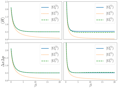
Figure 1: Comparison of the imaginary time dynamics for quantum, semiclassical and classical systems, in the cases of quadratic and quartic Hamiltonians. All quantities are given in natural units using $\hbar=k_{B}=1$. In both cases, the expected energy of the system is distinguished by the zero-point energy present in the quantum and semiclassical evolutions. Finally, the uncertainty relation in position and momentum is clearly respected in the quantum and semiclassical system, while in the classical system it approaches zero, reflecting the zero energy classical ground state.

VIII Non-linearity in waveoperator dynamics

There exist a number of phenomena whose description incorporates non-linear models, such as Bose-Einstein condensates [69], or wavefunction collapse [70]. A natural question to ask is therefore whether the waveoperator and density matrix representations may differ in the degree of non-linearity of their dynamics. There are in fact a number of scenarios in which a linear evolution in either $\hat{\rho}$ of $\hat{\Omega}$ leads to a non-linear evolution in the complementary representation. Here we provide two conjugate examples of this phenomenon.

First, let us consider a thermal state $\hat{\rho}(\beta)=\frac{1}{Z}{\rm e}^{-\beta\hat{H}}$. Representing this state as a waveoperator, we find

$$\ket{\Omega(\beta)}=\frac{1}{\sqrt{Z}}\sum_{j}{\rm e}^{-\frac{\beta}{2}\hat{H}}\ket{E_{j}}\otimes\ket{E_{j}},$$ (51)

where $\ket{E_{j}}$ are eigenvectors of $\hat{H}$. Remarkably, this object is one of some importance in holography [71], as it may represent a black hole in AdS conformal field theories [72], and hence provide a platform for the study of many quantum phenomena in this context [73, 74]. In such a context it is known as the thermofield double (TFD) state, and questions of how to prepare this state are a focus of ongoing research [75]. One consequence of this has been the finding that for a harmonic oscillator of mass $m$ and frequency $\omega$, using

$$\hat{a}=\sqrt{\frac{m\omega}{2\hbar}}\left(\hat{\mathbf{x}}+i\frac{1}{m\omega}\hat{\mathbf{p}}\right),$$ (52)

the TFD may be written as [76]

$$\ket{\Omega(\beta)}=\frac{1}{\sqrt{1-{\rm e}^{-\beta\omega}}}\sum_{n}{\rm e}^{-\frac{1}{2}n\beta\omega}\ket{n}\otimes\ket{n}.$$ (53)

where $\ket{n}$ is a state in the second-quantised basis. In this instance, it is possible to express this normalised waveoperator as the unitary evolution of a two-mode squeezing Hamiltonian on the vacuum state. This is given by [76]:

$$\ket{\Omega(t)}={\rm e}^{-\frac{i}{\hbar}t\left(\hat{\mathbf{x}}\otimes\hat{\mathbf{p}}+\hat{\mathbf{p}}\otimes\hat{\mathbf{x}}\right)}\ket{0}\otimes\ket{0},$$ (54)

where

$$t=\frac{1}{2}\log\left(\frac{1+{\rm e}^{-\frac{1}{2}\beta\omega}}{1-{\rm e}^{-\frac{1}{2}\beta\omega}}\right).$$ (55)

Most interestingly, in the waveoperator framework this leads to a form of dynamics where (up to a phase) $\hat{\Omega}(0)=\hat{\rho}(0)=\ket{0}\bra{0}$, and the generator does not conform to the form specified by Eq. (12). This is due to the fact that this generator possesses non-trivial operators on both sides of the tensor product. Nevertheless, Eqs. (10a-10c) may be employed to depurify $\ket{\Omega(t)}$, leading to a real-time equation of motion describing thermalisation on the level of $\hat{\Omega}$ in the number basis:

$$i\hbar\partial_{t}\hat{\Omega}=\hat{\mathbf{p}}\hat{\Omega}\hat{\mathbf{x}}^{T}+\hat{\mathbf{x}}\hat{\Omega}\hat{\mathbf{p}}^{T}.$$ (56)

The sandwiching of $\hat{\Omega}$ between operators has important consequences for the corresponding dynamics of $\hat{\rho}$, namely that it becomes intrinsically non-linear. To demonstrate this we first define the similarity transformation

$$\bar{A}(\hat{\Omega})\equiv\bar{A}=\hat{\Omega}\hat{A}^{T}\hat{\Omega}^{-1}.$$ (57)

Note that for any finite temperature, the eigenvalues of $\hat{\Omega}$ will be $\{{\rm e}^{-\frac{\beta}{2}E_{j}}\}$. Given these are all non-zero, $\hat{\Omega}^{-1}$ is guaranteed to exist. The evolution of a thermal state in real-time for the density may then be described with:

$$i\hbar\partial_{t}\hat{\rho}=(\hat{\mathbf{x}}\bar{\mathbf{p}}+\hat{\mathbf{p}}\bar{\mathbf{x}})\hat{\rho}-\hat{\rho}(\bar{\mathbf{p}}^{\dagger}\hat{\mathbf{x}}\ +\bar{\mathbf{x}}^{\dagger}\hat{\mathbf{p}})$$ (58)

revealing that such a thermalising evolution has drastically different properties depending on the representation one chooses for the state.

There also exists a complementary scenario in which the non-linearity relationship between the two representations is reversed. If we consider a Lindblad equation of the form [39]

$$\partial_{t}\hat{\rho}=-\frac{i}{\hbar}\left[\hat{H},\hat{\rho}\right]+2\hat{L}\hat{\rho}\hat{L}^{\dagger}-\left\{\hat{L}^{\dagger}\hat{L},\hat{\rho}\right\},$$ (59)

we find that the structure of the $\hat{L}\hat{\rho}\hat{L}^{\dagger}$ term leads to a dissipative equation for $\hat{\Omega}$. Using a slightly modified definition $\bar{L}=\hat{\Omega}^{-1}\hat{L}\hat{\Omega}$, we obtain [33]

$$\partial_{t}\hat{\Omega}=-\frac{i}{\hbar}\left[\hat{H},\hat{\Omega}\right]+\hat{L}\hat{\Omega}\bar{L}^{\dagger}-\hat{L}^{\dagger}\hat{L}\hat{\Omega}$$ (60)

where once again a linear equation has been transformed into a non-linear one due to the presence of an operator-state-operator sandwich term in the linear dynamics.

IX Discussion

Here we have presented a novel representation of Hilbert space dynamics, where positivity is automatically preserved by performing dynamics on the square root of the density operator. One advantage of the present formalism is that it may be set in Hilbert space with a Schrödinger-like equation of motion. Consequently it is possible to use all of the highly efficient tools developed for these dynamics (e.g. tensor network algorithms) when performing waveoperator calculations. Furthermore, incorporating purification allows one to introduce the Bopp operators to this formalism. This has resulted in a phase space representation of the waveoperator, which in turn allows us to identify the Wigner function as the projection of the waveoperator onto phase space.

Practical applications of the waveoperator formalism are already extant. For example, it has been used to formulate a method of thermal density matrix minimisation used to successfully calculate the equilibrium density matrix of a 6912 atom silicon cell [47]. Furthermore, the structural advantages of the waveoperator representation have already inspired proposals for the simulation of Lindbladian dynamics in the context of quantum circuits [77] as well as machine-learning assisted quantum state estimation [53].

Taking the classical limit of the waveoperator formalism, we find that it corresponds to the KvN representation of classical dynamics. For quadratic Hamiltonians, this correspondence to classical dynamics is exact even before taking any $\hbar\to 0$ limit. This mirrors similar results to be found in the path integral and Wigner representations of dynamics for quadratic systems. In the former case, a saddle point approximation ensures only paths corresponding to the classical action contribute to the propagator, while the Moyal bracket operation evolving the quasiprobability $W(x,p)$ reduces to the Poisson bracket in the phase space representation.

When performing an analogous procedure in imaginary time, an $O(\hbar^{2})$ correction distinguishes quantum and classical quadratic systems, suggesting the most significant difference between the quantum and classical regime is in the ground state systems inhabit, rather than their real time dynamics (see [78]). A potential application of this new semiclassical expansion is in the calculation of tunnelling rates [79], which at present employ semiclassical path-integrals. One future avenue of research is to investigate how this is related to the semiclassical waveoperator, and what if any advantage the latter may possess. The fact that the semiclassical expansion of the imaginary time evolution exhibits a quadratic correction to the classical Hamiltonian is strikingly similar to another context in which the equilibrium state of a system is determined by a correction to its bare Hamiltonian. Specifically, when considering a system strongly coupled to an environment, its thermal state is described by a “Hamiltonian of mean force” that accounts for the environmental interaction. In those cases where this effective Hamiltonian is known [80, 81, 8, 82, 83], the correction to the bare Hamiltonian is also quadratic rather than linear. It is tempting to speculate that these two phenomena may be related to each other.

There are a number of potential extensions to this formalism. For instance, the introduction of commuting Bopp operators in previous sections relies on the canonical commutation relation in an infinite dimensional space of operators [84]. Finite dimensional Hilbert spaces are more restrictive and generally do not allow introducing the analogs of the Bopp operators with the desired commutation properties. Nevertheless, one might employ (for example) a Jordan-Schwinger map [85] to represent such a finite dimensional system. This would introduce an oscillator basis obeying canonical commutation relations in the continuum limit, and open a route to calculations analogous to those presented here. More generally, the hunt for novel efficient representations for interacting systems is one of the chief motivations for the development of the waveoperator formalism. Specifically, the fact that positivity is automatically preserved is of vital importance when attempting to construct a hybrid formalism, where a partial classical limit is taken on one part of an interacting system. The importance of developing such formalisms should not be understated, given that all our interactions with the quantum world must be mediated through essentially classical devices, which will themselves have a quantum backreaction. The growing sophistication of quantum technology demands we be able to accurately describe such phenomena via a quantum-classical hybrid. Traditionally however, such hybrid representations map to the quantum density operator $\hat{\rho}$, and the hybrid equations of motion derived (e.g. the Alexandrov-Gerasimenko-Kapral equation [48, 49, 86]) do not necessarily preserve the positivity of the state [21], calling into question the physicality of the dynamics. This remains an area of active research [87, 88, 89, 90, 91, 92], with quantum computational approaches to this problem already being explored [93]. It is our hope that the waveoperator formalism developed here will provide a useful tool in the ongoing development of hybrid system models.

- [1] William B. Case. Wigner functions and weyl transforms for pedestrians. American Journal of Physics, 76(10):937–946, 2008.
- [2] E. Wigner. On the quantum correction for thermodynamic equilibrium. Phys. Rev., 40:749–759, Jun 1932.
- [3] George Baker. Formulation of Quantum Mechanics Based on the Quasi-Probability Distribution Induced on Phase Space. Phys. Rev., 109(6):2198–2206, 1958.
- [4] Thomas Curtright, David Fairlie, and Cosmas Zachos. A concise treatise on quantum mechanics in phase space. World Scientific, New Jersey, 2014.
- [5] H. J. Groenewold. On the principles of elementary quantum mechanics. Physica, 12(7):405–460, 1946.
- [6] L S Schulman. Techniques and applications of path integration. Dover Books on Physics. Dover Publications, Mineola, NY, December 2005.
- [7] R. P. Feynman and F. L. Vernon. The theory of a general quantum system interacting with a linear dissipative system. Ann. Phys., 24:118, 1963.
- [8] Gerard McCaul, C. D. Lorenz, and L. Kantorovich. Partition-free approach to open quantum systems in harmonic environments: An exact stochastic liouville equation. Phys. Rev. B, 95:125124, Mar 2017.
- [9] G. McCaul, C. D. Lorenz, and L. Kantorovich. Driving spin-boson models from equilibrium using exact quantum dynamics. Phys. Rev. B, 97:224310, Jun 2018.
- [10] G. McCaul and Denys. I. Bondar. How to win friends and influence functionals: deducing stochasticity from deterministic dynamics. EPJST, 230:733–754, April 2021.
- [11] A.O. Caldeira and A.J. Leggett. Path integral approach to quantum Brownian motion. Physica A, 121(3):587–616, 1983.
- [12] G W Ford and M Kac. On the Quantum Langevin Equation. J. Stat. Phys., 46:803, 1987.
- [13] C W Gardiner. Quantum noise and quantum Langevin equations. IBM J. Res. Develop., 32:127, 1988.
- [14] K.L. Sebastian. The Classical Description of Scattering From a Quantum System. Chem. Phys. Lett., 81(1):14–16, 1981.
- [15] A.J. Leggett, S. Chakravarty, A.T. Dorsey, Matthew Fisher, Anupam Garg, and W. Zwerger. Dynamics of the dissipative two-state system. Rev. Mod. Phys., 59(1), 1987.
- [16] N G van Kampen. Derivation of the quantum Langevin equation. J. Molec. Liquids, 71:97, 1997.
- [17] John R. Klauder. The feynman path integral: An historical slice. In A Garden of Quanta, pages 55–76. WORLD SCIENTIFIC, 2003.
- [18] Denys I. Bondar, Renan Cabrera, Dmitry V. Zhdanov, and Herschel A. Rabitz. Wigner phase-space distribution as a wave function. Phys. Rev. A, 88(5), 2013.
- [19] Gerard McCaul and Denys I Bondar. Free to harmonic unitary transformations in quantum and Koopman dynamics*. Journal of Physics A: Mathematical and Theoretical, 55(43):434003, oct 2022.
- [20] Gerard McCaul, Alexander Pechen, and Denys I. Bondar. Entropy nonconservation and boundary conditions for hamiltonian dynamical systems. Phys. Rev. E, 99:062121, Jun 2019.
- [21] Denys I. Bondar, François Gay-Balmaz, and Cesare Tronci. Koopman wavefunctions and classical–quantum correlation dynamics. Proceedings of the Royal Society A: Mathematical, Physical and Engineering Sciences, 475(2229):20180879, September 2019.
- [22] B O Koopman. Hamiltonian Systems and Transformation in Hilbert Space. Proc. Nat. Acad. Sci., 17(5):315–318, 1931.
- [23] Joshua Wilkie and Paul Brumer. Quantum-classical correspondence via liouville dynamics. i. integrable systems and the chaotic spectral decomposition. PRA, 55:27–42, Jan 1997.
- [24] Joshua Wilkie and Paul Brumer. Quantum-classical correspondence via liouville dynamics. ii. correspondence for chaotic hamiltonian systems. PRA, 55:43–61, Jan 1997.
- [25] E. C. G. Sudarshan. Interaction between classical and quantum systems and the measurement of quantum observables. Pramana, 6(3):117–126, Mar 1976.
- [26] David Viennot and Lucile Aubourg. Schrödinger–koopman quasienergy states of quantum systems driven by classical flow. J. Phys. A, 51(33):335201, jul 2018.
- [27] Manaka Okuyama and Masayuki Ohzeki. Quantum speed limit is not quantum. PRL, 120:070402, Feb 2018.
- [28] Abhijit Sen, Shailesh Dhasmana, and Zurab K Silagadze. Free fall in KvN mechanics and Einstein’s principle of equivalence. Annals of Physics, 422:168302, 2020.
- [29] Shailesh Dhasmana, Abhijit Sen, and Zurab K Silagadze. Equivalence of a harmonic oscillator to a free particle and Eisenhart lift. Annals of Physics, 434, 2021.
- [30] Shailesh Dhasmana Abhijit Sen, Bikram Keshari Parida and Zurab K. Silagadze. Eisenhart lift of Koopman-von Neumann mechanics. Journal of Geometry and Physics, 185:104732, 2023.
- [31] A D Bermúdez Manjarres. The schwinger action principle for classical systems. Journal of Physics A: Mathematical and Theoretical, 54(41):414003, September 2021.
- [32] A D Bermúdez Manjarres. Operational classical mechanics: holonomic systems. Journal of Physics A: Mathematical and Theoretical, 55(40):405201, September 2022.
- [33] Loïc Joubert-Doriol, Ilya G. Ryabinkin, and Artur F. Izmaylov. Non-stochastic matrix schrödinger equation for open systems. The Journal of Chemical Physics, 141(23):234112, 2014.
- [34] Armin Uhlmann. Parallel transport and “quantum holonomy” along density operators. Rep. Math. Phys., 24(2):229–240, October 1986.
- [35] Joachim J. Włodarz. On quantum mechanical phase-space wave functions. J. Chem. Phys., 100(10):7476–7480, May 1994.
- [36] S. Gheorghiu-Svirschevski. Nonlinear quantum evolution with maximal entropy production. Physical Review A, 63(2):022105, 2001.
- [37] Gian Paolo Beretta. Nonlinear model dynamics for closed-system, constrained, maximal-entropy-generation relaxation by energy redistribution. Physical Review E, 73(2):026113, 2006.
- [38] Gian Paolo Beretta. Nonlinear extensions of schrödinger–von neumann quantum dynamics: A set of necessary conditions for compatibility with thermodynamics. Modern Physics Letters A, 20(13):977–984, April 2005.
- [39] Gerard McCaul, Kurt Jacobs, and Denys I. Bondar. Fast computation of dissipative quantum systems with ensemble rank truncation. Phys. Rev. Research, 3:013017, Jan 2021.
- [40] C. Le Bris and P. Rouchon. Low-rank numerical approximations for high-dimensional Lindblad equations. Physical Review A, 87(2):022125, February 2013.
- [41] S. Finazzi, A. Le Boité, F. Storme, A. Baksic, and C. Ciuti. Corner-Space Renormalization Method for Driven-Dissipative Two-Dimensional Correlated Systems. Physical Review Letters, 115:080604, August 2015.
- [42] Kaelan Donatella, Zakari Denis, Alexandre Le Boité, and Cristiano Ciuti. Continuous-time dynamics and error scaling of noisy highly entangling quantum circuits. Physical Review A, 104(6):062407, Dec 2021.
- [43] B. Reznik. Unitary Evolution between Pure and Mixed States. Physical Review Letters, 76(8):1192–1195, February 1996.
- [44] A. Yahalom and R. Englman. A “square-root” method for the density matrix and its applications to Lindblad operators. Physica A, 371(2):368–386, 2006.
- [45] Cesare Tronci. Momentum maps for mixed states in quantum and classical mechanics. J. Geom. Mech, 11(4):639–656, 2019.
- [46] Igor Mezić. Spectral properties of dynamical systems, model reduction and decompositions. Nonlinear Dyn., 41(1-3):309–325, 2005.
- [47] Jacob M. Leamer, William Dawson, and Denys I. Bondar. Positivity preserving density matrix minimization at finite temperatures via square root, 2023.
- [48] I. V. Aleksandrov. The Statistical Dynamics of a System Consisting of a Classical and a Quantum Subsystem. Zeitschrift für Naturforschung A, 36(8), 1981.
- [49] V. I. Gerasimenko. Dynamical equations of quantum-classical systems. Theor. Math. Phys., 50(1):49–55, January 1982.
- [50] A. Nocera, A. Polkovnikov, and A. E. Feiguin. Unconventional fermionic pairing states in a monochromatically tilted optical lattice. Phys. Rev. A, 95:023601, Feb 2017.
- [51] G. McCaul, Christopher Orthodoxou, Kurt Jacobs, George H Booth, and Denys I Bondar. Controlling arbitrary observables in correlated many-body systems. Physical Review A, 101(5):053408, 2020.
- [52] G. McCaul, Christopher Orthodoxou, Kurt Jacobs, George H Booth, and Denys I Bondar. Driven imposters: Controlling expectations in many-body systems. Physical Review Letters, 124(18):183201, 2020.
- [53] Sanjaya Lohani, Brian T Kirby, Michael Brodsky, Onur Danaci, and Ryan T Glasser. Machine learning assisted quantum state estimation. Machine Learning: Science and Technology, 1(3):035007, July 2020.
- [54] Mark Wilde. Quantum information theory. Cambridge University Press, Cambridge, UK ; New York, second edition edition, 2017.
- [55] A Raab. On the Dirac–Frenkel/McLachlan variational principle. Chemical Physics Letters, 319(5):674–678, 2000.
- [56] J. v. Neumann. Uber einen satz von herrn m. h. stone. Ann. Math., 33(3):567–573, 1932.
- [57] Fritz Bopp. La mécanique quantique est-elle une mécanique statistique classique particulière ? Ann. Henri Poincaré, 15(2):81–112, 1956.
- [58] MOSM Hillery, Robert F O’Connell, Marlan O Scully, and Eugene P Wigner. Distribution functions in physics: Fundamentals. Phys. Rep., 106(3):121–167, 1984. Publisher: Elsevier.
- [59] D Zueco and I Calvo. Bopp operators and phase-space spin dynamics: application to rotational quantum Brownian motion. Journal of Physics A: Mathematical and Theoretical, 40(17):4635, apr 2007.
- [60] Renan Cabrera, Denys I. Bondar, Kurt Jacobs, and Herschel A. Rabitz. Efficient method to generate time evolution of the Wigner function for open quantum systems. Phys. Rev. A, 92(4), 2015.
- [61] Denys I. Bondar, Andre G. Campos, Renan Cabrera, and Herschel A. Rabitz. Efficient computations of quantum canonical Gibbs state in phase space. Physical Review E, 93(6), 2016.
- [62] Maximilian Ćirić, Denys I Bondar, and Ole Steuernagel. Exponential unitary integrators for nonseparable quantum Hamiltonians. Eur. Phys. J. Plus, 2023.
- [63] Denys I. Bondar, Renan Cabrera, Robert R. Lompay, Misha Yu. Ivanov, and Herschel A. Rabitz. Operational Dynamic Modeling Transcending Quantum and Classical Mechanics. Phys. Rev. Lett., 109(19), 2012.
- [64] Clarence W. Rowley, Igor Mezić, Baghari Shevin, Philipp Schlatter, and Dan S. Henningson. Spectral analysis of nonlinear flows. Journal of Fluid Mechanics, 641:115–127, 2009.
- [65] Igor Mezić. Analysis of fluid flows via spectral properties of the koopman operator. Annual Review of Fluid Mechanics, 45(1):357–378, 2013.
- [66] Milan Korda and Igor Mezić. Linear predictors for nonlinear dynamical systems: Koopman operator meets model predictive control. Automatica, 93:149–160, 2018.
- [67] A A Kirillov. Geometric Quantization, pages 139–176. Springer Berlin Heidelberg, Berlin, Heidelberg, 2001.
- [68] Marcus Berg and Cécile DeWitt-Morette. On Certain Unitary Representations of an Infinite Group of Transformations. WORLD SCIENTIFIC, 2001.
- [69] Dustin R Lindberg, Naceur Gaaloul, Lev Kaplan, Jason R Williams, Dennis Schlippert, Patrick Boegel, Ernst-Maria Rasel, and Denys I Bondar. Asymmetric tunneling of bose–einstein condensates. Journal of Physics B: Atomic, Molecular and Optical Physics, 56(2):025302, jan 2023.
- [70] L. Bonci, P. Grigolini, R. Roncaglia, and D. Vitali. Nonlinear schrödinger equation and wave-function collapse: An unreliable consequence of the semiclassical approximation. Phys. Rev. A, 47:3538–3545, May 1993.
- [71] Juan Maldacena. The large-n limit of superconformal field theories and supergravity. International Journal of Theoretical Physics, 38(4):1113–1133, 1999.
- [72] Juan Maldacena. Eternal black holes in anti-de sitter. Journal of High Energy Physics, 2003(04):021, apr 2003.
- [73] Ahmed Almheiri, Donald Marolf, Joseph Polchinski, Douglas Stanford, and James Sully. An apologia for firewalls. Journal of High Energy Physics, 2013(9), September 2013.
- [74] Leonard Susskind. Er=epr, ghz, and the consistency of quantum measurements. Fortschritte der Physik, 64(1):72–83, 2016.
- [75] Cheng-Ju Lin, Zhi Li, and Timothy H. Hsieh. Entanglement renormalization of thermofield double states. Phys. Rev. Lett., 127:080602, Aug 2021.
- [76] Shira Chapman, Jens Eisert, Lucas Hackl, Michal P. Heller, Ro Jefferson, Hugo Marrochio, and Robert C. Myers. Complexity and entanglement for thermofield double states. SciPost Phys., 6:034, 2019.
- [77] Dhrumil Patel and Mark M. Wilde. Wave matrix lindbladization i: Quantum programs for simulating markovian dynamics. Open Systems & Information Dynamics, 30(02), June 2023.
- [78] Endre Kajari, NL Harshman, EM Rasel, Stig Stenholm, Georg Süssmann, and Wolfgang P Schleich. Inertial and gravitational mass in quantum mechanics. Applied Physics B, 100(1):43–60, 2010.
- [79] D. Maile, S. Andergassen, W. Belzig, and G. Rastelli. Exponential speedup of incoherent tunneling via dissipation. Phys. Rev. Res., 3:033019, Jul 2021.
- [80] Yiu-Fung Chiu, Aidan Strathearn, and Jonathan Keeling. Numerical evaluation and robustness of the quantum mean-force gibbs state. Phys. Rev. A, 106:012204, Jul 2022.
- [81] Federico Cerisola, Marco Berritta, Stefano Scali, Simon A. R. Horsley, James D. Cresser, and Janet Anders. Quantum-classical correspondence in spin-boson equilibrium states at arbitrary coupling, 2022.
- [82] A. S. Trushechkin, M. Merkli, J. D. Cresser, and J. Anders. Open quantum system dynamics and the mean force gibbs state. AVS Quantum Science, 4(1):012301, 2022.
- [83] Harry J D Miller. Hamiltonian of Mean Force for Strongly-Coupled Systems, pages 531–549. Springer International Publishing, Cham, 2018.
- [84] Gerhard C. Hegerfeldt. On canonical commutation relations and infinite-dimensional measures. Journal of Mathematical Physics, 13(1):45–50, 1972.
- [85] J J Sakurai and Jim J Napolitano. Modern Quantum Mechanics. Pearson Education, Philadelphia, PA, 2 edition, July 2010.
- [86] Raymond Kapral and Giovanni Ciccotti. Mixed quantum-classical dynamics. J. Chem. Phys., 110(18):8919–8929, 1999.
- [87] Raymond Kapral. Progress in the theory of mixed quantum-classical dynamics. Annual Review of Physical Chemistry, 57(1):129–157, 2006. PMID: 16599807.
- [88] Wayne Boucher and Jennie Traschen. Semiclassical physics and quantum fluctuations. Phys. Rev. D, 37:3522–3532, Jun 1988.
- [89] Raymond Kapral and Giovanni Ciccotti. Mixed quantum-classical dynamics. The Journal of Chemical Physics, 110(18):8919–8929, 1999.
- [90] Steve Nielsen, Raymond Kapral, and Giovanni Ciccotti. Mixed quantum-classical surface hopping dynamics. The Journal of Chemical Physics, 112(15):6543–6553, 2000.
- [91] François Gay-Balmaz and Cesare Tronci. Evolution of hybrid quantum–classical wavefunctions. Physica D: Nonlinear Phenomena, 440:133450, 2022.
- [92] Giovanni Manfredi, Antoine Rittaud, and Cesare Tronci. Hybrid quantum-classical dynamics of pure-dephasing systems*. Journal of Physics A: Mathematical and Theoretical, 56(15):154002, mar 2023.
- [93] Daniel Bultrini and Oriol Vendrell. Towards mixed quantum-classical dynamics on quantum computers, 2023. arXiv:2303.11375.