Effects of detuning on $\mathcal{PT}$-symmetric, tridiagonal, tight-binding models

Abstract

Non-Hermitian, tight-binding $\mathcal{PT}$-symmetric models are extensively studied in the literature. Here, we investigate two forms of non-Hermitian Hamiltonians to study the $\mathcal{PT}$-symmetry breaking thresholds and features of corresponding surfaces of exceptional points (EPs). They include one-dimensional chains with uniform or 2-periodic tunnelling amplitudes, one pair of balanced gain and loss potentials $\Delta\pm\i\gamma$ at parity-symmetric sites, and periodic or open boundary conditions. By introducing a Hermitian detuning potential, we obtain the dependence of the $\mathcal{PT}$-threshold, and therefore the exceptional-point curves, in the parameter space of detuning and gain-loss strength. By considering several such examples, we show that EP curves of a given order generically have cusp-points where the order of the EP increases by one. In several cases, we obtain explicit analytical expressions for positive-definite intertwining operators that can be used to construct a complex extension of quantum theory by re-defining the inner product. Taken together, our results provide a detailed understanding of detuned tight-binding models with a pair of gain-loss potentials.

1 Introduction

Central to the axioms of quantum theory is the Hermiticity of the Hamiltonian, as it guarantees a unitary description of time evolution. Unitary time evolution only applies to isolated quantum systems. When a small quantum system interacts with the environment, the resulting dynamics for the reduced density matrix of the system is, typically, decoherence inducing. Under mild conditions such as a Markovian bath, this dynamics is described by a completely positive trace preserving (CPTP) map that is generated by the Lindblad equation [26, 50]. In recent years, non-Hermitian Hamiltonians have been extensively studied due to their emergence as effective descriptions of classical systems with gain and loss [38]. In the truly quantum domain, it has been shown that they emerge from Lindblad equation through post-selection where trajectories with quantum jumps are eliminated [62]. Examples of phenomena modelled by non-Hermitian Hamiltonians vary from gain and loss in photonics [16, 27, 67, 17], radioactive decay in nuclear systems [73, 20, 21], and renormalization in quantum field theories [47, 48, 40, 7].

Of particular interest in the study of non-Hermitian Hamiltonians are those with an antilinear symmetry. A system whose time evolution is governed by Hamiltonian with an antilinear symmetry exhibits time reversal symmetry [81]. A Hamiltonian with an antilinear symmetry has eigenvalues which are purely real or occur in complex conjugate pairs, because if $\lambda$ is an eigenvalue of that operator, then $\lambda^{*}$ also satisfies the characteristic equation. This feature - pairing of complex-conjugate eigenvalues - is often used to reflect systems with balanced loss and gain. Additionally, if a Hamiltonian exhibits unbroken antilinear symmetry, so that all of its eigenspaces are invariant under the same symmetry, the Hamiltonian’s spectrum is real [3]. For historical reasons, the linear and complex-conjugation parts of the antilinear symmetry are called parity and time-reversal symmetries respectively. In our models of $n$-site graphs, the state space is the Hilbert space $\mathbb{C}^{n}$, and the actions of parity and time-reversal operators are given by

$$\mathcal{P}_{n}e_{k} =e_{\overline{k}}$$ (1)

$$\mathcal{T}e_{k} =e_{k},$$ (2)

where $(e_{k})_{j}=\delta^{k}_{j}$ is the canonical basis for $\mathbb{C}^{n}$, $\delta$ is the Kronecker delta, and $\overline{k}=n+1-k$. Hamiltonians $H$ which are $\mathcal{PT}$-symmetric in this sense satisfy the constraint $H_{pq}=H^{*}_{\overline{p}\overline{q}}$ and are referred to as centrohermitian [46].

Given a $\mathcal{PT}$-symmetric Hamiltonian which depends on a set of parameters, the $\mathcal{PT}$-symmetry is unbroken for a subset of parameter space, the boundary of which consists exceptional points. Exceptional points (EPs) are spots in parameter space where the number of distinct eigenvalues (and corresponding eigenvectors) decreases [41]. We define the order of an EP to be the number of coalescing eigenvectors (irrespective of the algebraic multiplicity of corresponding eigenvalue) at the EP, and refer to an $k$-th order EP as an EP$k$.

An equivalent condition for the existence of an antilinear symmetry for $H$ is pseudo-Hermiticity [58, 75, 74]. Pseudo-Hermitian operators are those such that there is an Hermitian intertwining operator, $M=M^{\dagger}$, satisfying

$$H=M^{-1}H^{\dagger}M.$$ (3)

In the case where $M$ is positive definite, we refer to it as a metric operator, and $H$ is called quasi-Hermitian [14, 71]. A finite dimensional matrix has real eigenvalues if and only if it’s quasi-Hermitian [15, 59, 57, 61]. Furthermore, the metric operator defines an inner product for which a quasi-Hermitian operator is self-adjoint. Thus, quasi-Hermitian operators can be realized as observables in a fundamental extension of quantum theory to self-adjoint but non-Hermitian Hamiltonians [71]. On the other hand, if non-Hermitian Hamiltonians are considered an effective description, where loss of unitarity is not prohibited, one uses the Dirac-inner product to obtain observables and predictions, and the intertwining operators take the role of time invariants [9].

Given a pair of Hamiltonian $H$ and metric $M$, the metric for all similar Hamiltonians $S^{-1}HS$ can be constructed as [45],

$$(H,M)\leftrightarrow(H^{\prime},M^{\prime})=(S^{-1}HS,M^{\prime}=S^{\dagger}MS).$$ (4)

Notably, choosing $S=M^{-1/2}$ implies $M^{\prime}=\mathbb{1}$ and therefore $H^{\prime\dagger}=H^{\prime}$, i.e. an equivalent Hermitian Hamiltonian exists for all quasi-Hermitian Hamiltonians with bijective metric operators [82, 60].

The models in this paper are special cases of transpose-symmetric tridiagonal matrices over $\mathbb{C}^{n}$ with perturbed corners,

$$H_{ij} =z_{i}\delta^{i}_{j}+t_{j}\delta^{i}_{j+1}+t_{i}\delta^{j}_{i+1}+\delta^{i}_{\bar{j}}(t_{L}\delta^{i}_{1}+t_{R}\delta^{i}_{n})$$

$$=\begin{pmatrix}z_{1}&t_{1}&0&\dots&0&t_{L}\\ t_{1}&z_{2}&t_{2}&\ddots&\ddots&0\\ 0&t_{2}&z_{3}&\ddots&\ddots&\vdots\\ \vdots&\ddots&\ddots&\ddots&t_{n-2}&0\\ 0&\ddots&\ddots&t_{n-2}&z_{n-1}&t_{n-1}\\ t_{R}&0&\dots&0&t_{n-1}&z_{n}\end{pmatrix},$$ (5)

where $z_{i},t_{L},t_{R}\in\mathbb{C}$ and $t_{i}\in\mathbb{R}$.

$\mathcal{PT}-$symmetric variants of eq. 5 have been well explored [44, 32, 8, 37, 36, 72, 35, 64, 90, 28, 88, 89, 69, 87, 43, 33, 49, 84, 76, 55]. Numerous examples of eq. 5 have closed form solutions for the spectrum, an incomplete list includes [68, 18, 51, 85, 22, 86, 83, 11, 34, 23, 42, 13, 1]. Due to the well-known similarity transformation between generic tridiagonal matrices and their transpose-symmetric counterparts, displayed in [70, 36], the results of this report readily generalize to tridiagonal matrices which are not transpose symmetric, such as the Hatano-Nelson model [29].

2 Tight-binding models

The results of this paper can be categorized into three groups. The first two groups pertain to two special cases of matrices of the form eq. 5, and the last group pertains to generic features of exceptional points of bivariate matrix polynomials. These results are now described in order.

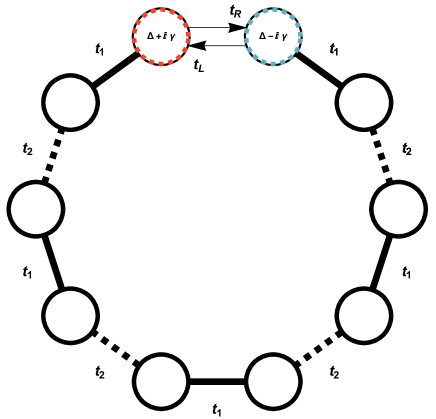
Figure 1: Graphical representation of the two cases of eq. 5 studied in this report, for $n=6$ (open chain, top) and $N=10$ (closed, SSH chain, bottom) respectively. The first case of an open chain with nearest neighbour defects is studied in [37], and the second case of an SSH chain with non-Hermitian defects on the boundary is studied in section 4.

The types of matrices studied in the first two groups of results are graphically depicted in fig. 1. In the first case, we consider a general Hermitian chain on an even lattice with open boundary conditions and non-Hermitian perturbations on the central two sites. In the second case, we consider a Su-Schrieffer-Heeger (SSH) chain with a pair non-Hermitian perturbations at the edges of the chain. The diagonal elements of $H$ are assumed to be real-valued everywhere except at a pair of mirror-symmetric sites, $(m,\overline{m})$ with $m\in\{1,\dots,n\}$. The sites $(m,\overline{m})$ will be referred to as defects. More explicitly,

$$z_{j}\in\mathbb{R}\,\,\forall j\notin\{m,\bar{m}\}.$$ (6)

To simplify select equations, we will denote the defect potentials as $z_{m}=\Delta+i\gamma$ and $z_{\overline{m}}=z_{m}^{*}=\Delta-i\gamma$. Here, without loss of generality, we take $\gamma\geq 0$; therefore, the site $m$ is the gain site and its mirror-symmetric site $\overline{m}$ is the loss site.

We will refer to the parameter $\Delta$ as detuning. To enforce $\mathcal{PT}$-symmetry, in most of the paper, we make the following assumptions on the model parameters:

$$t_{k} =t_{n-k}\in\mathbb{R}\setminus\{0\}$$

$$z_{k} =z_{\bar{k}}^{*}$$

$$t_{L} =t_{R}^{*}\in\mathbb{C}.$$ (7)

The spectrum of $H$, $\sigma(H)$, describing an open chain obeys the following symmetries:

$$\sigma(H(z_{i}))=-\sigma(H(-z_{i}))=\sigma(H(z_{i}^{*}))^{*},$$ (8)

where the first equality arises from the similarity transform $(-1)^{i+j}H_{ij}(z_{i})=-H_{ij}(-z_{i})$ [39, 77, 34] and the second equality arises from the $\mathcal{PT}$-symmetry of the Hamiltonian. When $z_{i}=0$, this symmetry is called chiral symmetry. Physically, it states that eigenvalues of $H$ arise in particle-hole symmetric pairs, and signals the existence of an operator $\Pi_{ij}=(-1)^{i}\delta_{ij}$ that anticommutes with the Hamiltonian.

2.1 Nearest Neighbour Defects

In section 3, we consider the case with nearest neighbour defects and open boundary conditions, i.e. $n=2m$, and $t_{L}=0=t_{R}$. In this case, the $\mathcal{PT}$-threshold is equal to the magnitude of the tunnelling amplitude $t_{m}>0$ between the nearest-neighbour defect sites. Note that $t_{m}>0$ can be chosen without loss of generality. For $\gamma\leq t_{m}$, the spectrum is purely real, and the EP occurs when $\gamma=\gamma_{\textrm{EP}}=t_{m}$ where the $2m$ dimensional system has exactly $m$ linearly independent eigenvectors. For $\gamma>t_{m}$, there are no real eigenvalues, i.e. the system has maximally broken $\mathcal{PT}$-symmetry [35].

In eq. 11, we obtain a one-parameter family of intertwining operators, $M$. A subset of positive-definite metric operators exists when the gain-loss strength satisfies $\gamma<t_{m}$. The intertwining operator is used to construct a so-called $\mathcal{C}$-symmetry of our transpose-symmetric Hamiltonian [4, 5]. Using the metric, we compute a similar Hermitian Hamiltonian, $H^{\prime}$, in eq. 18. Notably, the similarity-transformed Hermitian Hamiltonian is local. This contrasts with the generic cases of local $\mathcal{PT}-$ unbroken Hamiltonians, whose similar Hermitian operators are nonlocal [44].

Where the tunnelling is uniform, $t_{i}=t>0$, the spectrum of $H$ can be computed exactly for some special cases of defect potentials, summarized in table 1. Note that for a uniform chain, the choice of positive $t$ is always possible by a unitary transformation of the Hamiltonian. Since the eigenvalues of tridiagonal matrices always have geometric multiplicity equal to one [18], the cases in table (1) where $H$ has less than $n$ distinct eigenvalues are exceptional points.

Constraints	Eigenvalues of $H$
$z_{m}=\pm it$	$\left\{2t\cos\left(\dfrac{j\pi}{m+1}\right)\,\mid\,j\in\{1,\dots,m\}\right\}$
$z_{m}=(-1\pm i)t$	$\left\{2t\cos\left(\dfrac{2j\pi}{2m+1}\right)\,|\,j\in\{1,\dots,m\}\right\}$
$z_{m}=(1\pm i)t$	$\left\{2t\cos\left(\dfrac{(2j-1)\pi}{2m+1}\right)\,|\,j\in\{1,\dots,m\}\right\}$
$z_{m}=e^{\pm i\pi/3}t$	$\begin{array}[]{l}\left\{2t\cos\left(\dfrac{j\pi}{m+1}\right)\,|\,j\in\{1,\dots,m\}\right\}\cup\\ \left\{2t\cos\left(\dfrac{(2j-1)\pi}{2m+1}\right)\,|\,j\in\{1,\dots,m\}\right\}\end{array}$
$z_{m}=e^{\pm 2\pi i/3}t$	$\begin{array}[]{l}\left\{2t\cos\left(\dfrac{j\pi}{m+1}\right)\,|\,j\in\{1,\dots,m\}\right\}\cup\\ \left\{2t\cos\left(\dfrac{2j\pi}{2m+1}\right)\,|\,j\in\{1,\dots,m\}\right\}\end{array}$

Table 1: Non-Hermitian cases where the spectrum of $H$ has a closed form solution, for an even, uniform lattice with open boundary conditions and nearest-neighbour defects. The entry in the first row was known to [34]. The eigenvectors can be constructed using the ansatz of [34] or by computing characteristic polynomials [24].

2.2 SSH Chain

Our second set of results pertain to a non-Hermitian perturbation of the SSH model with open boundary conditions and non-Hermitian defects at the edges of the chain ($m=1$). Mathematically, we assume the tunnelling amplitudes are 2-periodic, given by $t_{1},t_{2}>0$ respectively, and we set

$$z_{i}=0\,\,\forall i\notin\{m,\bar{m}\}$$ (9)

Note that the choice of positive $t_{1},t_{2}$ for an open chain is always possible by using a diagonal, unitary transform. The case with zero detuning was studied in [87, 43], additional non-Hermitian perturbations of the SSH chain can be found in [69, 33, 49, 84, 76, 55], and several special cases of the eigenvalue equation are exactly solvable [68, 18, 51, 85, 22, 83, 12, 34, 23]. The characteristic polynomial for even and odd SSH chains are presented in table 2, generalizing the results in [22, 64]. Several special cases of the eigenvalue equation are exactly solvable [68, 18, 51, 85, 22, 83, 86, 12, 34, 23, 56].

When $t_{2}<t_{1}$, i.e. the weak links are in the interior of the chain, the system is in the topologically trivial phase. When $t_{1}<t_{2}$, the weak-links are at the edges of the chain, thereby rendering the system in the topologically nontrivial phase. In the thermodynamic limit ($n\to\infty$), in topologically nontrivial phase with zero detuning, [43] demonstrated that the $\mathcal{PT}$-symmetry breaks at $\gamma=0$ due to the presence of edge states, eigenstates which are peaked at the edges of the chain and decay exponentially as one moves inwards. Thus, the uniform chain with $t_{1}=t_{2}$ marks the transition between topologically trivial and non-trivial phases. We will therefore refer to it as a critical SSH chain as well. When we place two defects with detuning in an SSH system, the constraints of proposition (3) yield $\sigma(H)\subset\mathbb{R}$, i.e. a $\mathcal{PT}$-unbroken phase. A subset of the $\mathcal{PT}$-unbroken domain includes

$$(\Delta^{2}+\gamma^{2}\leq t_{2}^{2}\leq t_{1}^{2})\vee(\Delta^{2}+\gamma^{2}=t_{2}^{2}\wedge\gamma^{2}<t_{1}^{2}).$$ (10)

A subset of the $\mathcal{PT}$-broken phase is given by eqs. 44 and 45.

Continuing with the case of the critical SSH chain, $t_{2}=t_{1}=t$, we expand upon the works of [44, 32, 90]. The set of exceptional points is determined analytically in eq. 56. Asymptotic expressions for this set are studied in the large detuning case, $\Delta/t\rightarrow\infty$, and we find the critical defect strength scales as $\gamma_{\textrm{EP}}/t\propto(\Delta/t)^{(n-2)}$. In the thermodynamic limit of $n\rightarrow\infty$, the $\mathcal{PT}-$unbroken region is numerically demonstrated to approach the union of a unit disk $|z_{1}|/t=1$ and the real axis $\gamma=0$.

For defects inside a uniform chain, instead of at its end-points, we find that a subset of the spectrum is independent of the defect strength $z_{m}$ whenever $m$ shares a nontrivial factor with $n+1$; this occurs because precisely the open-uniform-chain eigenfunctions have a node at defect location, thereby rendering the defect invisible to their energies.

Exceptional points occur when these eigenvalues are multiple roots of the characteristic polynomial. In general, these exceptional points do not coincide with the $\mathcal{PT}$-symmetry breaking threshold, and the spectrum is generically complex in the vicinity of these exceptional points. Furthermore, as demonstrated in [64], when $\Delta=0$, there are even more constant eigenvalues.

3 Open Chain with Nearest Neighbour Impurities

In this section, we present analytical results for a non-uniform open chain with $n=2m$ and nearest neighbour defects $z_{m}=\Delta+i\gamma=z^{*}_{m+1}$. In particular we show that most of its properties are determined solely by the tunnelling amplitude $t_{m}>0$ connecting the two defect sites.

3.1 Intertwining operators and Inner product

Proposition 1.

A Hermitian intertwining operator $M$ for the matrix $H$ of eq. 5 in the $\mathcal{PT}$-symmetric case $t_{k}=t_{n-k}$ with nearest neighbour defects and open boundary conditions is given by the block matrix

$$M(Z_{m}) =\begin{pmatrix}\mathbb{1}_{m}&\frac{Z^{*}_{m}}{t_{m}}\mathcal{P}_{m}\\ \frac{Z_{m}}{t_{m}}\mathcal{P}_{m}&\mathbb{1}_{m}\end{pmatrix},$$ (11)

where $\mathbb{1}_{m}$ is the $m\times m$ identity matrix and $Z_{m}$ is a constant with arbitrary real part and $\Im Z_{m}=\gamma$. $M$ is positive-definite when $|Z_{m}|<t_{m}$. $M$ is the only intertwining operator for $H$ which is a sum of the identity matrix and an antidiagonal matrix.

Proof.

The proof is by induction. For $n=2$, the most general intertwining operator (modulo trivial multiplicative constant) is [80]

$$M=\begin{pmatrix}1&Z_{m}^{*}/t_{m}\\ Z_{m}/t_{m}&1\end{pmatrix}.$$ (12)

Suppose $M$ has the form eq. 11 when $n=n_{0}$. $M$ is the sum of a diagonal and an antidiagonal matrix, the following identity is a re-expression of eq. 3 for $n=n_{0}+1$,

$$\sum^{n_{0}}_{j=2}M_{i\,j}H_{jk}=\sum^{n_{0}}_{j=2}H^{{\dagger}}_{ij}M_{j\,k},\,\,\,\,\,\forall\,\,1<i,k<n.$$ (13)

Thus, for $n=n_{0}+1$, $M$ is a sum of a diagonal and an antidiagonal matrix and satisfies eq. 3 if and only if

$$\begin{pmatrix}M_{1,1}&M_{1,n}\\ M_{n,1}&M_{n,n}\end{pmatrix} =\begin{pmatrix}M_{2,2}&M_{2,n-1}\\ M_{n-1,2}&M_{n-1,n-1}\end{pmatrix},$$ (14)

which implies $M$ must have the form of eq. 11. Since $M$ is a direct sum of commuting $2\times 2$ block matrices, $M$ is positive-definite if and only if $|Z_{m}|<t_{m}$. That $M$ is the metric of $H$ was initially stated in [2]. Previous literature found the special case of $M$ for a uniform chain [88] and the special case with $n=2$ [60, 80]. ∎

We remind the reader of the similarity transform between the general tridiagonal model and the transpose symmetric variant, given in for instance [70, 36]. Using the mapping (4) with this similarity transform, the metric operator (11) is easily generalized to cases where the Hamiltonian is not transpose symmetric [36].

3.2 Equivalent Hermitian Hamiltonian

When the intertwining operator is postive-definite, i.e. the non-Hermitian Hamiltonian has purely real spectrum, we can construct an equivalent Dirac-Hermitian Hamiltonian as follows. In this section, we assume $|Z_{m}|<t_{m}$. An Hermitian Hamiltonian, $h=h^{\dagger}$, which is similar to $H$ is defined as

$$h: =\Omega H\Omega^{-1}=M^{1/2}HM^{-1/2},$$ (15)

where $\Omega=\sqrt{M}$ denotes the unique positive square root of $M$. Since the metric defined in eq. 11 is block diagonal, the non-unitary similarity transform $\Omega$ can explicitly be calculated as

$$\Omega =\begin{pmatrix}\frac{\alpha}{2}\mathbbm{1}_{m}&\frac{Z_{m}^{*}}{\alpha t_{m}}\mathcal{P}_{m}\\ \frac{Z_{m}}{\alpha t_{m}}\mathcal{P}_{m}&\frac{\alpha}{2}\mathbb{1}_{m}\end{pmatrix}=\frac{\alpha}{2}\mathbbm{1}_{2m}+\frac{1}{\alpha t_{m}}\left(\Re Z_{m}\sigma_{x}+\Im Z_{m}\sigma_{y}\right)\otimes\mathcal{P}_{m},$$ (16)

where $\alpha=\sqrt{1+|Z_{m}|/t_{m}}+\sqrt{1-|Z_{m}|/t_{m}}$. Thus, the equivalent Hermitian Hamiltonian for the non-uniform open chain is given by

$$h_{ij} =t^{\prime}_{i}\delta_{i+1,j}+{t^{\prime}_{i}}^{*}\delta_{i,j+1}+\Re z_{i}\delta_{i,j}$$ (17)

$$t^{\prime}_{i} :=\begin{cases}\sqrt{|t_{i}t_{n-i}|}&\,\text{if }i\neq m\\ \frac{\Re Z_{m}}{Z_{m}}t_{m}+i\frac{\Im Z_{m}}{Z_{m}}\sqrt{t_{m}^{2}-|Z_{m}|^{2}}&\,\text{if }i=m\end{cases}$$ (18)

Interestingly, this equivalent Hamiltonian remains tridiagonal, and is interpreted as local to a one-dimensional chain. This is in stark contrast to most other cases where the non-unitary similarity transform $\Omega$ generates long-range interactions thereby transforming a local, $\mathcal{PT}$-symmetric Hamiltonian $H$ with real spectra into an equivalent, non-local Hermitian Hamiltonian whose range of interaction diverges as one approaches the exceptional point degeneracy [44].

3.3 $\mathcal{C}$ Symmetry

Consider a pseudo-Hermitian matrix $H$ with two intertwining operators, $\eta_{1}$ and $\eta_{2}$. It is straightforward to show that $\eta_{2}^{-1}\eta_{1}$ commutes with $H$ [59]. Owing to the $\mathcal{PT}$-symmetry and transpose symmetry of $H$ with open boundary conditions, a particular operator which commutes with $H$ is

$$\mathcal{C}:=\frac{1}{\sqrt{t_{m}^{2}-\gamma^{2}}}\mathcal{P}M(\i\gamma)=\frac{1}{\sqrt{t_{m}^{2}-\gamma^{2}}}\left(t_{m}\mathbbm{1}_{2m}+\gamma\sigma_{y}\otimes\mathcal{P}_{m}\right),$$ (19)

In the domain where $H$ is $\mathcal{PT}$-unbroken and diagonalizable, the symmetry $\mathcal{C}$ is a Hermitian involution $\mathcal{C}^{2}=\mathbb{1}$ which commutes with $\mathcal{PT}$. Due to the $\mathcal{C}$ symmetry and non-degeneracy of $H$ [18], the eigenvectors of $H$ are elements of the eigenspaces of $\mathcal{C}$,

$$V_{\pm}=\text{span}\left\{t_{m}e_{k}+(-\i\gamma\pm\sqrt{t^{2}_{m}-\gamma^{2}})e_{\bar{k}}\,|\,k\in\{1,\dots,m\}\right\}.$$ (20)

The coalescence of $V_{+}$ and $V_{-}$ as one approaches $\gamma=t_{m}$ is a signature that this is an exceptional point.

3.4 Complexity of spectrum

The central result of this section is that if $\gamma>t_{m}$, every eigenvalue has a nonzero imaginary part. This generalizes the result of [35] to the case with finite detuning and site-dependent tunnelling profiles. Suppose a given eigenvalue, $\lambda\in\sigma(H)$, is real, $\lambda\in\mathbbm{R}$. Since the geometric multiplicity of $\lambda$ is one [18], the corresponding eigenstate, $|\psi\rangle=\sum_{k=1}^{2m}\psi_{k}e_{k}$, is also an eigenstate of the antilinear operator $\mathcal{PT}$. As a consequence of the eigenvalue equations, without loss of generality, the eigenstate can be taken to be real for all sites on the left half of the lattice, $\psi_{k}\in\mathbbm{R}\,\forall k\leq m$. By $\mathcal{PT}$ symmetry, there exists a phase $\chi\in[0,2\pi)$ such that $\psi_{\bar{k}}e^{i\chi}=\psi_{k}\,\forall k\leq m$. With these observations in mind, the eigenvalue equations at the nearest-neighbour defect sites $(m,m+1)$ are equivalent to

$$\begin{pmatrix}(z_{m}-\lambda)\psi_{m}+t_{m-1}\psi_{m-1}&t_{m}\psi_{m}\\ t_{m}\psi_{m}&(z_{m+1}-\lambda)\psi_{m}+t_{m-1}\psi_{m-1}\end{pmatrix}\begin{pmatrix}1\\ e^{i\chi}\end{pmatrix}=0.$$ (21)

For this matrix to have a nontrivial kernel, its determinant must vanish. However, if $\gamma>t_{m}$, the determinant is strictly positive. The contradictory assumption was taking $\lambda\in\mathbbm{R}$, thus, every eigenvalue is has a nonzero imaginary part when $\gamma>t_{m}$.

3.5 Degree of $\mathcal{PT}-$Symmetry Breaking

The reality of the spectrum of $H$ for $\gamma<|t_{m}|$ follows from the positive-definite nature of the explicitly constructed intertwining operator eq. 11 in that domain. When $\gamma=t_{m}$, the intertwining operator $M$ is no longer positive definite, but is positive semi-definite. Consequently, in this section we demonstrate at at $\gamma=t_{m}$ the spectrum of $H$ is still real, but $H$ is no longer diagonalizable.

Proposition 2.

When $\gamma=|t_{m}|$, $H$ has exactly $m$ orthogonal eigenvectors corresponding to real eigenvalues with algebraic multiplicity equal to two and geometric multiplicity equal to one.

Proof.

First, we prove that $H$ has at most $m$ linearly independent eigenvectors. To achieve this goal, consider the characteristic polynomial of $H$. Denoting $H_{i}$ as the matrix formed by taking the first $i$ rows and columns of $H$, denoting $p_{A}$ as the monic characteristic polynomial of a matrix $A$, and applying the linearity property of determinants, we find

$$p_{H}(\lambda)=(\gamma^{2}-t_{m}^{2})p_{H_{m-1}}^{2}(\lambda)+\left[\Delta p_{H_{m-1}}(\lambda)+p_{H_{m}}(\lambda)\right]^{2}.$$ (22)

When $\gamma=t_{m}$, $p_{H}$ is the square of a monic polynomial of degree $m$. Thus, in this case, each eigenvalue of $H$ has an algebraic multiplicity of at least two. Since the geometric multiplicity of every eigenvalue of $H$ equals one [18], there are at most $m$ linearly independent eigenvectors.

One simple proof that $H$ has at least $m$ eigenvectors when $\gamma^{2}=t_{m}^{2}$ follows from applying theorem 1 of [15] to the positive semi-definite intertwiner $M$. We provide an alternative proof here. Consider the action of $H$ on $\ker M$. An orthonormal basis of $\ker M$ is

$$\ker M =\text{span}\{\tilde{e}_{j}\,|\,j\in\{1,\dots,m\}\}$$ (23)

$$\tilde{e}_{j} =\frac{\i\gamma}{\sqrt{2}t_{m}}e_{j}+\frac{1}{\sqrt{2}}e_{\bar{j}}.$$ (24)

Then

$$H\tilde{e}_{j} =\begin{cases}t_{1}\tilde{e}_{2}&\text{ if }j=1\\ t_{j-1}\tilde{e}_{j-1}+t_{j}\tilde{e}_{j+1}&\text{ if }j\in\{2,\dots,m-1\}\\ t_{m-1}\tilde{e}_{m-1}&\text{ if }j=m\end{cases}.$$ (25)

Thus, $\ker M$ is an invariant subspace of $H$. Define $\tilde{H}:\ker M\to\ker M$ by the condition $\tilde{H}(v)=H(v)$ for all $v\in\ker M$. Equation (25) implies that $\tilde{H}$ is Hermitian, so it has $m$ orthogonal eigenvectors whose corresponding eigenvalues are real. These eigenvectors are also of $H$, demonstrating $H$ has at least $m$ eigenvectors corresponding to real eigenvalues. We emphasize that proposition (2) is valid for arbitrary, $\mathcal{PT}$-symmetric tunnelling profiles and finite detuning. ∎

3.6 Exact spectra for detuned uniform chain

In this section, we outline the process by which the exact spectra presented in table 1 are obtained for a uniform ($t_{j}=t>0$) chain with a pair of detuned defects $z_{m}=z^{*}_{\bar{m}}$. Generalizing the works of [68, 51, 34], the eigensystem in this case was computed in [64]. For our purposes, we need the (rescaled) characteristic polynomial,

$$P_{n,m}(x;z^{\prime}): =\text{det}(2xI-H/t)$$

$$=U_{n}\left(x\right)-(z^{\prime}_{m}+z^{\prime}_{\bar{m}})U_{n-m}\left(x\right)U_{m-1}\left(x\right)$$

$$+z^{\prime}_{m}z^{\prime}_{\bar{m}}U_{n-2m}\left(x\right)U_{m-1}\left(x\right)^{2}=0,$$ (26)

where $x=\lambda/2t$ is the dimensionless eigenvalue of $H$, and denote scaled defect strength by $z^{\prime}_{m}=z_{m}/t$, and the Chebyshev polynomial of second kind is denoted by $U_{n}(x)=\sin\left[(n+1)\arccos x\right]/\sin(\arccos x)$. The special cases with closed form spectrum in table 1 can be derived from simplifying eq. 26 with the identity

$$U_{2m}(x) =U^{2}_{m}(x)-U^{2}_{m-1}(x).$$ (27)

If the polynomials $U_{n}(x),U_{n-m}(x),$ and $U_{n-2m}(x)$ share a common zero, then corresponding to this zero is an eigenvalue of $H$ which is independent of the complex defect strength $z_{m},z_{\bar{m}}$. Similarly, in the zero-detuning case, $z_{m}=-z_{\bar{m}}$, $H$ has an eigenvalue independent of $z_{m}$ if $U_{n}(x)$ and $U_{n-2m}(x)$ share a common zero. It also follows that this eigenvalue is real since $\sigma(H)$ is real in the Hermitian limit. Thus, a subset of the spectrum is

$$g:=\begin{cases}\gcd(2m,n+1)&\text{ if }z_{m}=-z_{\bar{m}}\\ \gcd(m,n+1)&\text{ otherwise}\end{cases}$$ (28)

$$\sigma(H)\supseteq\left\{2t\cos\left(\pi\frac{k}{g}\right):k\in\{1,\dots g-1\}\right\}.$$ (29)

We also point out to the reader that $x=0$ is solution of the characteristic polynomial independent of $z_{m}$ whenever $n$ is odd and $\Delta=0$. It represents the zero-energy state that is decouped from the defect potentials due to its vanishing weigths on the defect sites.

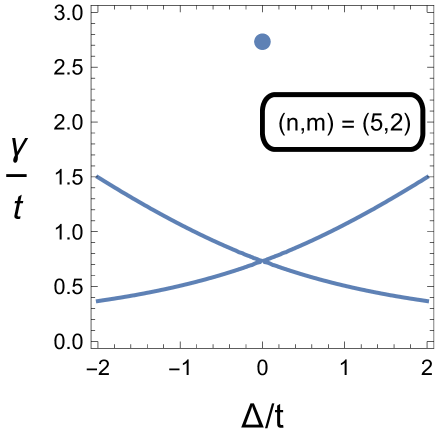
Figure 2: Exceptional points (blue) of $H$ with $t_{i}=t$, $t_{L}=t_{R}=0$, $(n,m)=(5,2)$ as a function of the defect strength $\gamma/t$ and $\Delta/t$. At small $\gamma/t$, all five eigenvalues are real. The points $z_{m}=0+i\gamma=i(\sqrt{3}\pm 1)t$ are a crunode $(-)$ and an acnode $(+)$, respectively, with eigenvalues $\sigma(H)=\{0,-(\pm 1)^{1/2}3^{1/4},(\pm 1)^{1/2}3^{1/4}\}$. In addition to the zero eigenvalue, the remaining eigenvalues at $z_{m}=i(\sqrt{3}\pm 1)t$ have algebraic multiplicity 2 and geometric multiplicity 1.

Figure 2 shows the exceptional points for an $n=5$ site chain with defects at sites $m=2$ and $\bar{m}=4$. Although this is a uniform chain, since it has odd number of sites, the nearest defects are still two sites apart. Therefore, the exact results presented earlier for nearest-neighbour defects do not apply.

4 Non-Hermitian SSH Model with farthest defects

In this section, we enforce the parametric restrictions $t_{k}=t_{k^{\prime}}>0$ for $k^{\prime}=k\mod 2$ and defects on sites $m=1$ and $\bar{m}=n$. Our key results regard the number of real eigenvalues and the set of exceptional points.

4.1 Eigensystem Solution

The characteristic polynomial of the tridiagonal matrix corresponding to the Hermitian SSH model with open boundary conditions [19, Remark 5] is given by

$$D_{n}(t_{1},t_{2}): =(t_{1}t_{2})^{-\lfloor n/2\rfloor}\text{det}\begin{pmatrix}\lambda&-t_{1}&0&\dots\\ -t_{1}&\lambda&-t_{2}&\ddots\\ 0&-t_{2}&\lambda&-t_{1}\\ \vdots&\ddots&-t_{1}&\ddots\\ \end{pmatrix}$$ (30)

$$=\begin{cases}\lambda U_{k}(Q)&\text{ if }n=2k+1\\ U_{k}Q+\frac{t_{2}}{t_{1}}U_{k-1}(Q)&\text{ if }n=2k.\end{cases}$$ (31)

where

$$Q:=\frac{\lambda^{2}-(t_{1}^{2}+t_{2}^{2})}{2t_{1}t_{2}}.$$ (32)

To generalize this result to a non-Hermitian model ($z_{k}\neq 0$) with corner elements ($t_{L},t_{R}\neq 0$), we use the linearity property of determinants for rows and columns. Computing the characteristic polynomial for $H(z_{1},z_{n},t_{L},t_{R})$ can thus be reduced to the problem of finding $D_{n}(t_{1},t_{2})$. The result is summarized in table 2. The case for an open chain, $t_{L}=0=t_{R}$, was known to [22], and the case $t_{1}=t_{2}$ was known to [86].

Constraints	$(t_{1}t_{2})^{-\lfloor n/2\rfloor}\text{det}(\lambda I-H)$
$n=2k$	$\begin{array}[]{l}U_{k}(Q)+\left(\dfrac{z_{1}z_{n}-t_{L}t_{R}}{t_{2}^{2}}\right)U_{k-2}(Q)\\ +\left(\dfrac{t_{2}^{2}-\lambda(z_{1}+z_{n})+z_{1}z_{n}-t_{L}t_{R}}{t_{1}t_{2}}\right)U_{k-1}(Q)-\dfrac{t_{L}+t_{R}}{t_{2}}\end{array}$
$n=2k+1$	$\begin{array}[]{l}\left(\lambda-z_{1}-z_{n}\right)U_{k}(Q)-(t_{L}+t_{R})\\ +\left(\dfrac{\lambda(z_{1}z_{n}-t_{L}t_{R})-z_{1}t_{1}^{2}-z_{n}t_{2}^{2}}{t_{1}t_{2}}\right)U_{k-1}(Q)\end{array}.$

Table 2: Characteristic polynomial of $H(z_{1},z_{n},t_{L},t_{R})$ for even and odd SSH chains.

To find the eigenvector corresponding to a root of table 2 we express eigenvalue equation as a linear recurrence relation,

$$t_{i}\psi_{i+1}=\lambda\psi_{i}-t_{i-1}\psi_{i-1} \forall i\in\{2,\dots n-1\}.$$ (33)

Solving this linear recurrence relation is equivalent to computing the $2\times 2$ matrix power,

$$\begin{pmatrix}\psi_{2k}\\ \psi_{2k-1}\end{pmatrix} =\begin{pmatrix}\frac{(\lambda^{2}-t_{2}^{2})}{t_{1}t_{2}}&-\frac{\lambda}{t_{2}}\\ \frac{\lambda}{t_{2}}&-\frac{t_{1}}{t_{2}}\end{pmatrix}^{k-1}\begin{pmatrix}\psi_{2}\\ \psi_{1}\end{pmatrix}.$$ (34)

Using the following expression for powers of invertible $2\times 2$ matrix $A$ [66],

$$A^{k} =(\det A)^{k/2}\left[-U_{k-2}(y)\mathbbm{1}_{2}+U_{k-1}(y)\frac{A}{\sqrt{\det A}}\right],$$ (35)

where $y=\text{tr}A/2\sqrt{\det A}$ is the dimensionless argument, we arrive at

$$\begin{pmatrix}\psi_{2k}\\ \psi_{2k-1}\end{pmatrix} =\begin{pmatrix}U_{k-1}(Q)+\frac{t_{1}}{t_{2}}U_{k-2}(Q)&-\frac{\lambda}{t_{2}}U_{k-2}(Q)\\ \frac{\lambda}{t_{2}}U_{k-2}(Q)&-\left(\frac{t_{1}}{t_{2}}U_{k-2}(Q)+U_{k-3}(Q)\right)\end{pmatrix}\begin{pmatrix}\psi_{2}\\ \psi_{1}\end{pmatrix}$$ (36)

These results are valid for $2k\leq n$. In addition, by using the equations that relate $\psi_{1},\psi_{2},\psi_{n}$ with tunnelling $t_{L}$ and $\psi_{1},\psi_{n-1},\psi_{n}$ with tunnelling $t_{R}$, we get

$$\left[z_{1}-\lambda+\lambda\frac{t_{L}}{t_{2}}U_{m-2}(Q)\right]\psi_{1}=\left[t_{L}U_{m-1}(Q)+\frac{t_{L}t_{1}}{t_{2}}U_{m-2}(Q)-t_{1}\right]\psi_{2},$$ (37)

thereby determining the eigenvector modulo normalization. On the other hand, if the identity holds due to vanishing prefactors of $\psi_{1}$ and $\psi_{2}$, then the state corresponding to that $\lambda$ is doubly degenerate.

4.2 Eigenvalue Inclusion Results

This section is devoted to finding subsets of the complex plane which contain some or all of the eigenvalues of $H$. As a consequence, we will find a subset of the $\mathcal{PT}-$unbroken and $\mathcal{PT}$-broken domains. A subset of the $\mathcal{PT}$-unbroken domain is found by applying the intermediate value theorem to the characteristic polynomial. To simplify results, we define

$$\mu_{k}=|t_{1}+t_{2}e^{(2i\pi/n)k}|\geq 0$$ (38)

and denote the intervals with endpoints $(-1)^{s_{1}}(t_{1}+(-1)^{s_{2}}t_{2})$ and $(-1)^{s_{1}}\text{sgn}(t_{1}+(-1)^{s_{2}}t_{2})\mu_{1}$ with $s_{1},s_{2}\in\{0,1\}$ as $I((-1)^{s_{1}},(-1)^{s_{2}})$.

Proposition 3.

Consider an even chain with $n=2k$ and assume $t_{L}=-t_{R}$. This realization includes an open chain ($t_{L}=0=t_{R}$), a closed chain with purely imaginary, Hermitian coupling ($t_{L}=i|t|=-t_{R}$), and a closed, non-Hermitian chain ($t_{L}=-t_{R}\in\mathbb{R}$). If $t_{2}^{2}=z_{1}z_{n}-t_{L}t_{R}$, then

$$\sigma(H)=\left\{\pm\mu_{j}\,|\,1\leq j\leq k-1\right\}\cup\left\{\frac{z_{1}+z_{n}}{2}\pm\sqrt{t_{1}^{2}-t_{2}^{2}+\left(\frac{z_{1}+z_{n}}{2}\right)^{2}}\,\right\}.$$ (39)

If $t_{2}^{2}\neq z_{1}z_{n}-t_{L}t_{R}$, then the intervals $(\mu_{j+1},\mu_{j})$ and $(-\mu_{j},-\mu_{j+1})$ each contain one eigenvalue of $H$ for $1\leq j\leq(k-1)$. Constraining other parameters as specified below guarantees the existence of additional real eigenvalues in corresponding intervals,

$$1+k\left(1\pm_{2}\frac{t_{2}}{t_{1}}\right)\frac{\left(\Delta\mp_{1}t_{2}\right)^{2}+\gamma^{2}-t_{L}t_{R}}{t_{2}^{2}-\Delta^{2}-\gamma^{2}+t_{L}t_{R}}\geq 0\, \Rightarrow\,\sigma(H)\cap I(\pm_{1}1,\pm_{2}1)\neq\emptyset.$$ (40)

Proof.

We utilize an alternative expression to the characteristic polynomial. Using the identity

$$U_{n\pm 1}(x) =xU_{n}(x)\pm T_{n+1}(x),$$ (41)

where $T_{n}(x)$ is the Chebyshev polynomial of the first kind, $T_{n}(x)=\cos(n\arccos x)$, we can rewrite the characteristic polynomial, with $n=2k$, as

$$(t_{1}t_{2})^{-k}\text{det}(\lambda I-H) =T_{k}(Q)\left(1-\frac{z_{1}z_{n}-t_{L}t_{R}}{t_{2}^{2}}\right)-\frac{t_{L}+t_{R}}{t_{2}}$$

$$+\left(1+\frac{z_{1}z_{n}-t_{L}t_{R}}{t_{2}^{2}}\right)QU_{k-1}(Q)$$

$$+\left(\frac{t_{2}^{2}-\lambda(z_{1}+z_{n})+z_{1}z_{n}-t_{L}t_{R}}{t_{1}t_{2}}\right)U_{k-1}(Q)$$ (42)

Equation (39) follows from the observation that the first term of eq. 42 vanishes when $z_{1}z_{n}-t_{L}t_{R}=t_{2}^{2}$ and the second one vanishes when $t_{R}=-t_{L}$.

Next, consider the case $z_{1}z_{n}-t_{L}t_{R}\neq t_{2}^{2}$, and $n\geq 4$. The sign of the characteristic polynomial is different at the endpoints of the intervals $(\mu_{j},\mu_{j+1})$ and $(-\mu_{j+1},-\mu_{j})$ for all $j\in\{1,\dots,k-2\}$, so there exists a real eigenvalue of $H$ inside each of these intervals. The inequalities of eq. 40 follow from considering the sign of the characteristic polynomial at the endpoints of the intervals $I(\pm_{1}1,\pm_{2}1)$. ∎

The inequalities of eq. 40 when $t_{1}^{2}=t_{2}^{2}$ were known to [83, eq. (63-64)] while special cases of eq. 39 were presented in [68, 83, 44, 28]. Two of the inequalities eq. 40 are satisfied if $t_{2}^{2}\geq z_{1}z_{n}-t_{L}t_{R}=\Delta^{2}+\gamma^{2}-t_{L}t_{R}$, and all four inequalities are satisfied if $t_{1}\geq t_{2}$. Thus, $\sigma(H)\subset\mathbb{R}$ when $\Delta^{2}+\gamma^{2}-t_{L}t_{R}\leq t_{2}^{2}\leq t_{1}^{2}$.

Now we focus on the complex part of the spectrum. A subset of the $\mathcal{PT}$-broken domain is found as an application of the Brauer-Ostrowski ovals theorem [10, 65, 78]. Let $C(w_{1},w_{2};b)=\{w\in\mathbb{C}\,|\,|w-w_{1}|\cdot|w-w_{2}|\leq b\}$ denote a Cassini oval. By the Brauer-Ostrowski ovals theorem, all eigenvalues of $H$ are elements of the union of Cassini ovals, specifically

$$\sigma(H)\subseteq C(0,0;(t_{1}+t_{2})^{2})\cup C(0,z_{n};(t_{1}+t_{2})(t_{1}+|t_{R}|))\cup$$

$$C(z_{1},0;(t_{1}+t_{2})(t_{1}+|t_{L}|))\cup C(z_{1},z_{n};(t_{1}+|t_{L}|)(t_{1}+|t_{R}|)).$$ (43)

Since eigenvalues are continuous in the arguments of a continuous matrix function [41], if the union of the Cassini ovals in eq. 43 contains disjoint components, then each component contains at least one eigenvalue of $H$. In particular, if both of the inequalities

$$\left[|z_{1}|^{2}-(t_{1}+t_{2})^{2}\right]\gamma >|z_{1}|(t_{1}+|t_{L}|)(t_{1}+|t_{R}|),$$ (44)

$$2(r_{1}+t_{2}) <\left(|z_{1}|+\sqrt{|z_{1}|^{2}-4t_{1}^{2}-4\min\{|t_{L}|^{2},|t_{R}|^{2}\}}\right)$$ (45)

hold, then there exist disjoint components containing the points $z_{1}$ and $z_{n}=z_{1}^{*}$, implying the existence of at least two eigenvalues with nonzero imaginary parts.

4.3 Topological Phases of the even SSH chain with open boundary conditions

The eigenvectors of tight-binding models are characterized as either bulk or edge states based on how their inverse participation ratio scales with the chain size $n$ [36, 79]. Roughly, the bulk eigenstates are spread over most of the chain irrespective of the chain size, whereas edge states remain exponentially localized within a few sites even with increasing chain size. Observing

$$U_{n}(Q)=\frac{(Q+\sqrt{Q^{2}-1})^{n+1}-(Q-\sqrt{Q^{2}-1})^{n+1}}{2\sqrt{Q^{2}-1}},$$ (46)

we see the sequence of Chebyshev polynomials $U_{n}(Q)$ is oscillatory in $n$ for $|Q|\leq 1$ and scales exponentially with $n$ otherwise. Thus, existence of non-trivial topological phase with edge-localized states is equivalent to existence of eigenvalues which do not satisfy $|Q|\leq 1$. Thus, for this particular model, in the thermodynamic limit, the $\mathcal{PT}$-broken phase is equivalent to topologically nontrivial phase, as complex eigenvalues correspond to edge states.

4.4 Exceptional Points for the Critical SSH Chain

This section will locate the exceptional points of a uniform chain with defect potentials at the edges of an open lattice, so $t_{1}=t=t_{1}$. Given that the spectrum is exactly solvable in the case $z_{1}z_{n}=t^{2}$, we will assume $z_{1}z_{n}\neq t^{2}$ for this section.

The theory of resultants [25], applied to the characteristic polynomial $P(\lambda):=\text{det}(\lambda I-H)$, can be used to analytically determine the exceptional points of $H$. The resultant of two monic polynomials $f(x)$ and $g(x)$ with degrees $F$ and $G$ respectively can be defined as

$$\text{Res}_{x}(f,g) :=\prod^{\text{F}}_{i=1}g(x_{i})$$ (47)

where $\{x_{i}\}$ denotes the full set of roots of $f(x)$. The resultant vanishes if and only if its inputs share one or more roots [25]. In particular, the Hamiltonian $H$ has $k$ degenerate eigenvalues if and only if

$$\text{Res}_{\lambda}\left(P(\lambda),\frac{\partial^{i}P(\lambda)}{\partial\lambda^{i}}\right) =0\,\,\,\forall i\in\{1,\dots,k\}$$ (48)

$$\text{Res}_{\lambda}\left(P(\lambda),\frac{\partial^{k+1}P(\lambda)}{\partial\lambda^{k+1}}\right) \neq 0.$$ (49)

For the generic Hamiltonian, eqs. 48 and 49 are not satisfied for all parameters. Thus, in the generic case where only two (but not more) eigenvalues become degenerate, finding the EPs reduces to locating Hamiltonian parameters and an eigenvalue $\lambda_{0}$ such that

$$P(\lambda_{0}) =0=\frac{\partial P(\lambda)}{\partial\lambda}\Bigr{|}_{\lambda=\lambda_{0}}.$$ (50)

Computation of the general set of exceptional points reduces to finding the resultants in eqs. 48 and 49, derived from the characteristic polynomial $P_{n,1}$, eq. 26. The following properties of Chebyshev polynomials are used in subsequent calculations [63, 54, 53]

$$U_{n}(x) =2xU_{n-1}(x)-U_{n-2}(x),$$ (51)

$$\frac{dU_{n}}{dx} =\dfrac{(n+1)U_{n+1}(x)-nxU_{n}(x)}{1-x^{2}},$$ (52)

$$U_{n-1}\left(\frac{x+x^{-1}}{2}\right) =\frac{x^{n}-x^{-n}}{x-x^{-1}}.$$ (53)

The resultant of Chebyshev polynomials, calculated in [31, 52], shows that $\text{Res}\left(U_{n},U_{m}\right)\neq 0$ if $n$ and $m$ are co-prime and $\text{Res}\left(U_{n},U_{m}\right)=0$ if $n+1$ and $m+1$ are not co-prime. Due to the denominator $(1-x^{2})$ in the derivative of Chebyshev polynomials, eq. 53, it is convenient to work with $\text{Res}_{x}\left[P_{n,1}(x),(1-x^{2})dP_{n,1}(x)/dx\right]$ instead. To simplify this resultant, we use the identity $(1-x^{2})dP_{n,1}/dx=AP_{n,1}(x)+BU_{n-1}(x)$ where the $H$-dependent prefactors are given by

$$A(x) =n\frac{z^{\prime}_{1}+z^{\prime}_{n}-x(1+z^{\prime}_{1}z^{\prime}_{n})}{1-z^{\prime}_{1}z^{\prime}_{n}},$$ (54)

$$B(x) =2z^{\prime}_{1}z^{\prime}_{n}-x(z^{\prime}_{1}+z^{\prime}_{n})+(n+1)(1-z^{\prime}_{1}z^{\prime}_{n})+\frac{n(2x-z^{\prime}_{1}-z^{\prime}_{n})(2xz^{\prime}_{1}z^{\prime}_{n}-z^{\prime}_{1}-z^{\prime}_{n})}{1-z^{\prime}_{1}z^{\prime}_{n}}.$$ (55)

We remind the reader that the dimensionless defect strengths $z^{\prime}_{1},z^{\prime}_{n}$ in eqs. 54 and 55 are scaled by the uniform tunnelling amplitude $t$. Denoting the two roots of $B(x)$, eq. 55, as $b_{\pm}$, we obtain the resultant,

$$P_{n,1}(1)P_{n,1}(-1)\text{Res}_{x}\left(P_{n,1},\frac{dP_{n,1}}{dx}\right)\propto P_{n,1}(b_{+})P_{n,1}(b_{-}).$$ (56)

The resultant of eq. 56 vanishes if and only if $(z_{1},z_{n})$ is an exceptional point, with a single eigenvector, as long as the corresponding $H(z_{1},z_{n})$ is not Hermitian; if $H$ is Hermitian, then a vanishing resultant merely denotes a doubly-degenerate eigenvalue which supports two linearly independent eigenvectors. Note that eq. 56 does not yield insight for parameters $(z_{1},z_{n})$ that are tuned such that $P_{n,1}(\pm 1)=0$ for arbitrary $n$. However, we readily identify $P_{n,1}(\pm 1)=0$ if and only if $(n-1)z^{\prime}_{1}z^{\prime}_{n}\mp n(z^{\prime}_{1}+z^{\prime}_{n})+(n+1)=0$. In this case, exceptional points occur when $\pm 1$ is a double root of $P_{n}$, which occurs when $z^{\prime}_{1}={z^{\prime}_{n}}^{*}\in\left\{\frac{2-2n^{2}+i\sqrt{3n^{2}-3}}{(2n-1)(n-1)},\frac{2n^{2}-2+i\sqrt{3n^{2}-3}}{(2n-1)(n-1)}\right\}$.

This analytical expression also allows us to extract the dependence of the $\mathcal{PT}$-threshold value on the detuning, where $z_{1}=\Delta+i\gamma=z_{n}^{*}$. Using the expansion of the roots $b_{\pm}$ of the quadratic expression $B(x)=0$, eq. 55, in the limit $\Delta/t\gg 1$, and applying the method of dominant balance [6] gives

$$P_{n,1}(b_{+})P_{n,1}(b_{-})=\frac{\Delta^{2}}{n^{2}t^{2}}\left(1-\frac{1}{n}\right)^{n-2}\left[\frac{\gamma^{2}\Delta^{2(n-2)}}{t^{2n}}-1\right]+O(1,\gamma^{4}\Delta^{2n-4}).$$ (57)

It follows that the EPs determined by vanishing of eq. 57 satisfy $\gamma_{\text{EP}}(\Delta)=t^{n-1}/\Delta^{(n-2)}$ in the limit $\Delta/t\gg 1$. Figure 3 shows the numerically obtained EP contours for this problem in the $(\gamma/t,\Delta/t)$ plane with varying chain sizes $n$. When $n=2$, the $\Delta$ term contributes $\mathbbm{1}_{2}$ to the Hamiltonian and therefore does not change the threshold $\gamma_{\text{EP}}(\Delta)=t$.

The zero detuning threshold is [44, 32]

$$\gamma_{EP}(0)/t=\begin{cases}\sqrt{1+1/n}&\text{if }n\text{ is odd}\\ 1&\text{if }n\text{ is even}\end{cases}.$$ (58)

This exceptional point corresponds to a zero mode with geometric multiplicity one, and algebraic multiplicity which is three in the odd case and two in the even case.

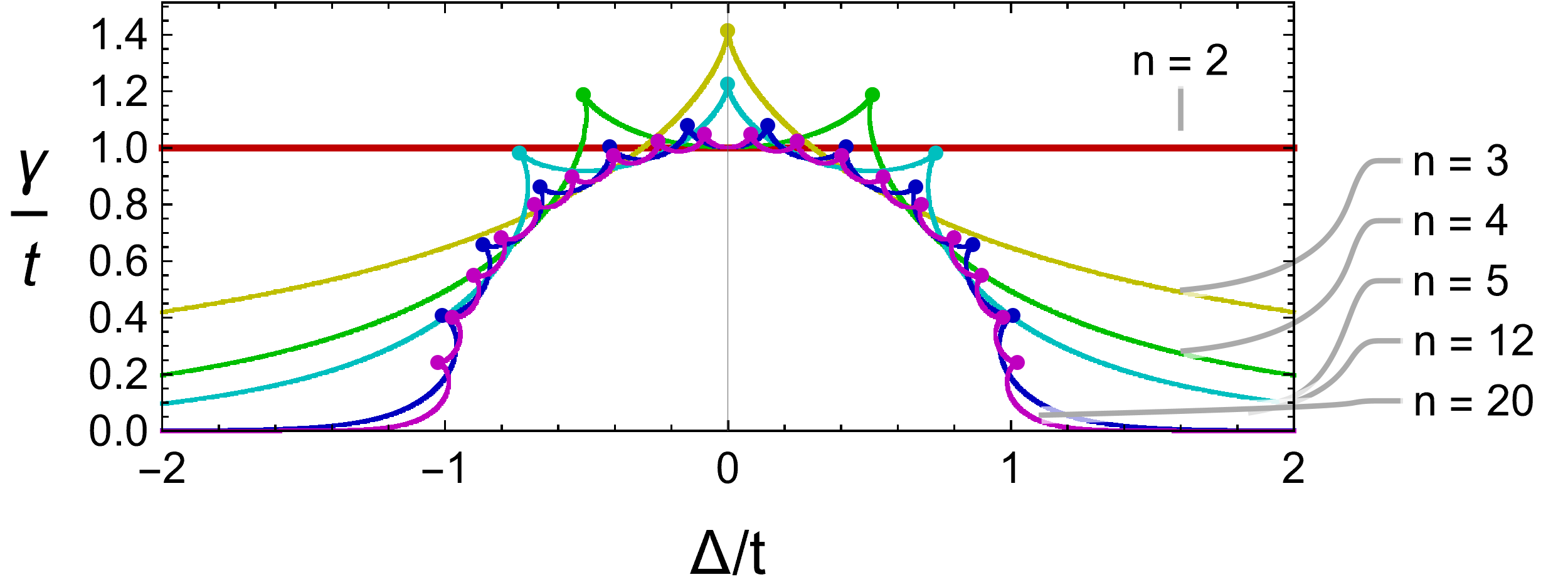
Figure 3: Exceptional points (EPs) of a uniform, n-site, tight-binding, open chain, eq. 5, with defects $z_{1}=\Delta+i\gamma=z_{n}^{*}$ at its end points. $\mathcal{PT}$-symmetry breaks as one passes from below the EP contour to above. Each contour, an algebraic curve, has $(n-2)$ cusp singularities marked by filled circles. The cusp singularities correspond to third order exceptional points (EP3s) while the rest of the contours are exceptional points of second order (EP2s). Our numerics suggest that the EP contours are one-to-one functions of $\text{arg}(z_{1})$. As $n\rightarrow\infty$, the $\mathcal{PT}$-unbroken region approaches the unit disk $|z_{1}|/t=1$. The curves for $n=3,4,5$ are in [69].

4.5 Locating EP3s in contours of EP2s

As a consequence of the Newton-Puiseux theorem, given an $n\times n$ matrix which is a polynomial in one parameter, $\theta$, the eigenvalues, $\lambda_{i}$ can be expanded as a Puiseux series in $\theta$,

$$\lambda_{i}(\theta)=\lambda_{i}(\theta_{0})+\sum^{\infty}_{j=1}\epsilon_{ij}(\theta_{0})(\theta-\theta_{0})^{j/k(i)},$$ (59)

where $k(i)\in\mathbb{N}$. To guarantee a real spectrum in a neighbourhood of $\theta_{0}$, as is the case for a Hermitian matrix, the condition $k(i)=1$ is necessary and sufficient. On the other hand, if $\lambda_{i}(\theta_{0})$ is an EP of order $N$, then $k(i)=N$. The sensitivity of the spectrum to perturbations in $\theta_{0}$ is quantified by

$$\tau(\theta_{0}):=\max\{\epsilon_{i1}(\theta_{0})|k(i)=\sup(k(1),\cdots,k(n))\}$$ (60)

If $\theta_{0}$ parametrizes an EP contour which contains EPs with different values of $k$, the corresponding $\tau(\theta_{0})$ must diverge as one approaches a point with an increased $k$ value. We now consider perturbations of the eigenvalues of the $\mathcal{PT}$-symmetric case of $H$ for $m=1$ at the exceptional points, fig. 3. If the tangent to an algebraic curve of EPs is unique and 2-directional, then perturbations along the tangents to the contour have $k=1$ and result in real eigenvalues. In orthogonal direction, there exists exactly one pair of eigenvalues which displays a real-to-complex-conjugtes transition, so $k=2$. Only at the cusp singularities is $k=3$ satisfied. To show this, in fig. 4 we plot the coefficient of the square-root term $\tau(\theta)$ as a function of angle in the $(\Delta,\gamma)$ plane, i.e. $\theta=\text{arg}(z_{1})$, for $\theta\in[0,\pi/2]$. As is expected, $\tau(\theta)$ diverges at non-uniformly distributed cusp points.

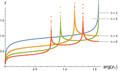
Figure 4: Coefficient $\tau(\theta)$ of the square-root term in the perturbative expansion of EP2 degenerate eigenvalue as a function of $\theta=\text{arg}(z_{1})$. Since $\tau(\theta)=\tau(\pi-\theta)=\tau(-\theta)$, the range is confined to $[0,\pi/2]$. The divergences are signatures of EP3s where the eigenvalue expansion is expressed through cube-roots instead of square-roots.

To exlore the generality of our observation, we next consider the SSH Hamiltonian with detuned defects $(z_{1},z_{n})$ as a function of three dimensionless parameters, $\Delta/t_{2},\gamma/t_{2},$ and $t_{1}/t_{2}$. In this case, the EPs form a 2-dimensional surface, with ridges that correspond to EP3s. At $\Delta=0$, these ridges intersect giving rise to EP4 cusp singularities.

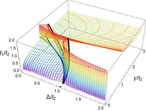
(a)

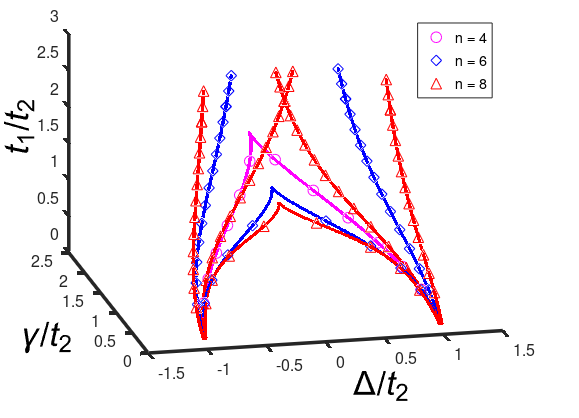
(b)

Figure 5: (a) EPs of an open SSH chain with end-defects and $n=8$. The domain satisfying the inequalities of eq. 40 lies in between this EP2 surface and the $\gamma=0$ plane. Ridges of this surface correspond to EP3s, plotted in fig. 5(b). As one passes through this surface along a ray originating at $\gamma=0$, we pass from the $\mathcal{PT}-$unbroken region to the $\mathcal{PT}$-broken region. The $\mathcal{PT}$-broken region is a subset of the topologically nontrivial phase, marked by the existence of edge states. (b) Contours of EP3s from fig. 5(a) show cusp singularities at $\Delta=0$ and are fourth order exceptional points (EP4s).

5 Generic Structure of Exceptional Surfaces

In this section, we use a perturbative argument to demonstrate that EPs of third order generically occur at cusp singularities of curves second order EPs.

Consider a Hamiltonian which is polynomial in $d\geq 2$ complex parameters, $H:\mathbb{C}^{d}\rightarrow\text{End}(\mathbb{C}^{n})$ with a third-order exceptional point, $x_{0}\in\mathbb{C}^{d}$. At this EP3, there exists at least one root, $\lambda_{0}$, whose algebraic multiplicity increases by 2. Then the characteristic polynomial may be written

$$\text{det}(\lambda-H(x))=\sum_{i=0}^{n}p_{i}(x)(\lambda-\lambda_{0})^{i},$$ (61)

where the polynomials $p_{i}(x)$ satisfy $p_{i}(x_{0})=0\,\forall i<3$ and $p_{3}(x_{0})\neq 0$. As we perturb $x_{0}\rightarrow x_{0}+\delta x$, the first-order correction $\delta\lambda=\lambda-\lambda_{0}$ to the eigenvalue $\lambda_{0}$ is found by substituting the Taylor expansions of $p_{i}$ in eq. 61. To simplify future calculations, we will assume $p_{0}^{\prime}(x_{0})\neq 0$, so the eigenvalue near $\lambda_{0}$ is approximated by

$$p_{3}(x_{0})\delta\lambda^{3}+p_{2}(x)\delta\lambda^{2}+p_{1}(x)\delta\lambda+\left(p_{0}^{\prime}(x_{0})\cdot\delta x\right)\approx 0.$$ (62)

Consider a perturbation along a line in parameter space passing through the exceptional point. Explicitly, let this line be $\{\theta u\,|\,\theta\in\mathbb{R}\}$ for some $u\in\mathbb{C}^{d}$. Given $\delta x=\theta u$, a Puiseux series expansion for a subset of eigenvalues along this line is

$$\delta\lambda(\theta)\approx\begin{cases}\dfrac{(p_{0}^{\prime}(x_{0})\cdot u)^{1/3}}{p_{3}(x_{0})}\,\theta^{1/3}&\text{if }p_{0}^{\prime}(x_{0})\cdot u\neq 0\\ \dfrac{(p_{1}^{\prime}(x_{0})\cdot u)^{1/2}}{p_{3}(x_{0})}\,\theta^{1/2}&\text{if }p_{0}^{\prime}(x_{0})\cdot u=0\text{ and }p_{1}^{\prime}(x_{0})\cdot u\neq 0\\ \dfrac{(p_{2}^{\prime}(x_{0})\cdot u)}{p_{3}(x_{0})}\,\theta&\text{if }p_{0}^{\prime}(x_{0})\cdot u=p_{1}^{\prime}(x_{0})\cdot u=0\text{ and }p_{2}^{\prime}(x_{0})\cdot u\neq 0\end{cases}.$$ (63)

Notably, the order of the Puiseux series expansion decreases if the line spanned by $u$ is orthogonal to the normal vector of the surface $p_{0}=0$ at $x_{0}$.

The set of exceptional points near $x=x_{0}$ is approximated by the discriminant of eq. 62,

$$p_{1}^{2}p_{2}^{2}-4p_{0}p_{2}^{3}-4p_{1}^{3}p_{3}+18p_{0}p_{1}p_{2}p_{3}-27p_{0}^{2}p_{3}^{2}=0.$$ (64)

The point $\delta x=0$ is readily interpreted as a singular point of the affine algebraic variety of exceptional points approximated by eq. 64, since the derivatives of eq. 64 with respect to each coordinate $\delta x_{i}$ all vanish. The leading term in eq. 64 for small $\delta x_{i}$ is the $p_{0}^{2}p_{3}^{2}$ term. Assuming the leading term in the expansion of $p_{1}^{2}p_{2}^{2}-4p_{0}p_{2}^{3}-4p_{1}^{3}p_{3}+18p_{0}p_{1}p_{2}p_{3}$ is an odd function of $\theta$ for a perturbation along $\delta x=\theta u$, then the line determined by $p_{0}(x)\approx p_{0}^{\prime}(x_{0})\delta x=0$ is a one-directional tangent to the surface of exceptional points, so we can interpret the point $x=x_{0}$ as a cusp singularity [30].

6 Conclusion

Non-Hermitian, tridiagonal, finite-dimensional matrices with $\mathcal{PT}$-symmetry are particularly amenable to analytical treatment. They also model a vast variety of physically realizable classical and quantum systems with balanced gain and loss. Introducing just one pair of gain-loss defect potentials breaks translational symmetry in such models and makes them non-amenable to traditional, Fourier-space band-structure methods. However, experimentally implementing $O(n)$ balanced gain-loss pairs in an $n$-site chain is exceptionally challenging, if not impossible. Therefore, we have considered models with minimal non-Hermiticity that leads to $\mathcal{PT}$-symmetry, i.e. one pair of defect potentials at mirror-symmetric sites.

Our results include the explicit analytical expressions for various intertwinning operators, construction of equivalent Hermitian Hamiltonian in the $\mathcal{PT}$-exact phase, and analytical results for the EP contours in a uniform chain with detuned defects at the end points. We have shown that cusp points of contours of EPs correspond to EPs of one-higher order. Taken together, these results deepen our understanding of exceptional-point degeneracies in physically realizable models.

References

- [1] A. Alazemi, C. M. Fonseca and E. Kılıç “The spectrum of a new class of Sylvester-Kac matrices” In Filomat 35.12 National Library of Serbia, 2021, pp. 4017–4031 DOI: 10.2298/fil2112017a
- [2] J. L. Barnett “Nonlocality of observable algebras in quasi-Hermitian quantum theory” In J. Phys. A 54.29 IOP Publishing, 2021, pp. 295307 DOI: 10.1088/1751-8121/ac0732
- [3] C. M. Bender, S. Boettcher and P. N. Meisinger “PT-symmetric quantum mechanics” In J. Math. Phys. 40.5 AIP Publishing, 1999, pp. 2201–2229 DOI: 10.1063/1.532860
- [4] C. M. Bender, D. C. Brody and H. F. Jones “Complex extension of quantum mechanics” In Phys. Rev. Lett. 89.27 American Physical Society (APS), 2002, pp. 270401 DOI: 10.1103/physrevlett.89.270401
- [5] C. M. Bender, D. C. Brody and H. F. Jones “Erratum: Complex Extension of Quantum Mechanics [Phys. Rev. Lett. 89, 270401 (2002)]” In Phys. Rev. Lett. 92, 2004, pp. 119902 DOI: 10.1103/physrevlett.92.119902
- [6] C. M. Bender and S. A. Orszag “Advanced mathematical methods for scientists and engineers I: Asymptotic methods and perturbation theory” Springer Science & Business Media, 2013 DOI: 10.1007/978-1-4757-3069-2
- [7] C. M. Bender, S. F. Brandt, J. Chen and Q. Wang “Ghost busting: PT-symmetric interpretation of the Lee model” In Phys. Rev. D 71.2 American Physical Society (APS), 2005, pp. 025014 DOI: 10.1103/physrevd.71.025014
- [8] O. Bendix, R. Fleischmann, T. Kottos and B. Shapiro “Exponentially Fragile PT Symmetry in Lattices with Localized Eigenmodes” In Phys. Rev. Lett. 103.3 American Physical Society (APS), 2009, pp. 030402 DOI: 10.1103/physrevlett.103.030402
- [9] Z. Bian et al. “Conserved quantities in parity-time symmetric systems” In Phys. Rev. Res. 2.2 APS, 2020, pp. 022039 DOI: 10.1103/physrevresearch.2.022039
- [10] A. Brauer “Limits for the characteristic roots of a matrix. II.” In Duke Math. J. 14.1 Duke University Press, 1947 DOI: 10.1215/s0012-7094-47-01403-8
- [11] H.-W. Chang, S.-E. Liu and R. Burridge “Exact eigensystems for some matrices arising from discretizations” In Linear Algebra Appl. 430.4 Elsevier BV, 2009, pp. 999–1006 DOI: 10.1016/j.laa.2008.09.034
- [12] W. Chu “Fibonacci polynomials and Sylvester determinant of tridiagonal matrix” In Appl. Math. Comput. 216.3 Elsevier BV, 2010, pp. 1018–1023 DOI: 10.1016/j.amc.2010.01.089
- [13] W. Chu “Spectrum and eigenvectors for a class of tridiagonal matrices” In Linear Algebra Its Appl. 582 Elsevier BV, 2019, pp. 499–516 DOI: 10.1016/j.laa.2019.08.017
- [14] J. Dieudonné “Quasi-Hermitian operators” In Proc. Internat. Sympos. Linear Spaces (Jerusalem, 1960), Pergamon, Oxford 115122, 1961
- [15] M. P. Drazin and E. V. Haynsworth “Criteria for the reality of matrix eigenvalues” In Math. Z. 78.1 Springer ScienceBusiness Media LLC, 1962, pp. 449–452 DOI: 10.1007/bf01195188
- [16] R. El-Ganainy, K. G. Makris, D. N. Christodoulides and Z. H. Musslimani “Theory of coupled optical -symmetric structures” In Opt. Lett. 32.17 The Optical Society, 2007, pp. 2632 DOI: 10.1364/ol.32.002632
- [17] R. El-Ganainy et al. “Non-Hermitian physics and PT symmetry” In Nat. Phys. 14.1 Springer ScienceBusiness Media LLC, 2018, pp. 11–19 DOI: 10.1038/nphys4323
- [18] J. F. Elliott “The characteristic roots of certain real symmetric matrices”, 1953
- [19] L. Elsner and R. M. Redheffer “Remarks on band matrices” In Numer. Math. 10.2 Springer ScienceBusiness Media LLC, 1967, pp. 153–161 DOI: 10.1007/bf02174148
- [20] H. Feshbach “Unified theory of nuclear reactions” In Ann. Phys. 5.4 Elsevier BV, 1958, pp. 357–390 DOI: 10.1016/0003-4916(58)90007-1
- [21] H. Feshbach “A unified theory of nuclear reactions. II” In Ann. Phys. 19.2 Elsevier BV, 1962, pp. 287–313 DOI: 10.1016/0003-4916(62)90221-x
- [22] C. M. Fonseca “The characteristic polynomial of some perturbed tridiagonal k-Toeplitz matrices” In Appl. Math. Sci 1.2, 2007, pp. 59–67
- [23] C. M. Fonseca, S. Kouachi, D. A. Mazilu and I. Mazilu “A multi-temperature kinetic Ising model and the eigenvalues of some perturbed Jacobi matrices” In Appl. Math. Comp. 259 Elsevier BV, 2015, pp. 205–211 DOI: 10.1016/j.amc.2015.02.058
- [24] F. R. Gantmacher and M. G. Krein “Oscillation Matrices and Kernels and Small Vibrations of Mechanical Systems” American Mathematical Society, 2002 DOI: 10.1090/chel/345
- [25] I. M. Gelfand, M. Kapranov and A. Zelevinsky “Discriminants, Resultants, and Multidimensional Determinants” Birkhäuser Boston, 1994 DOI: 10.1007/978-0-8176-4771-1
- [26] V. Gorini “Completely positive dynamical semigroups of N-level systems” In J. Math. Phys. 17.5 AIP Publishing, 1976, pp. 821 DOI: 10.1063/1.522979
- [27] A. Guo et al. “Observation of -Symmetry Breaking in Complex Optical Potentials” In Phys. Rev. Lett. 103.9 American Physical Society (APS), 2009, pp. 093902 DOI: 10.1103/physrevlett.103.093902
- [28] C. Guo and D. Poletti “Solutions for bosonic and fermionic dissipative quadratic open systems” In Phys. Rev. A 95.5 APS, 2017, pp. 052107 DOI: 10.1103/physreva.95.052107
- [29] N. Hatano and D. R. Nelson “Localization Transitions in Non-Hermitian Quantum Mechanics” In Phys. Rev. Lett. 77.3 American Physical Society (APS), 1996, pp. 570–573 DOI: 10.1103/physrevlett.77.570
- [30] H. Hilton “Plane algebraic curves” Clarendon Press, 1920
- [31] D. P. Jacobs, M. O. Rayes and V. Trevisan “The Resultant of Chebyshev Polynomials” In Can. Math. Bull. 54.2 Canadian Mathematical Society, 2011, pp. 288–296 DOI: 10.4153/cmb-2011-013-1
- [32] L. Jin and Z. Song “Solutions of -symmetric tight-binding chain and its equivalent Hermitian counterpart” In Phys. Rev. A 80.5 American Physical Society (APS), 2009, pp. 052107 DOI: 10.1103/physreva.80.052107
- [33] L. Jin, P. Wang and Z. Song “Su-Schrieffer-Heeger chain with one pair of -symmetric defects” In Sci. Rep. 7.1 Springer ScienceBusiness Media LLC, 2017, pp. 1–9 DOI: 10.1038/s41598-017-06198-9
- [34] Y. N. Joglekar “Mapping between Hamiltonians with attractive and repulsive potentials on a lattice” In Phys. Rev. A 82.4 American Physical Society (APS), 2010, pp. 044101 DOI: 10.1103/physreva.82.044101
- [35] Y. N. Joglekar and J. L. Barnett “Origin of maximal symmetry breaking in even PT-symmetric lattices” In Phys. Rev. A 84.2 American Physical Society (APS), 2011, pp. 024103 DOI: 10.1103/physreva.84.024103
- [36] Y. N. Joglekar and A. Saxena “Robust -symmetric chain and properties of its Hermitian counterpart” In Phys. Rev. A 83.5 American Physical Society (APS), 2011, pp. 050101 DOI: 10.1103/physreva.83.050101
- [37] Y. N. Joglekar, D. Scott, M. Babbey and A. Saxena “Robust and fragile -symmetric phases in a tight-binding chain” In Phys. Rev. A 82.3 American Physical Society (APS), 2010, pp. 030103 DOI: 10.1103/physreva.82.030103
- [38] Y. N. Joglekar, C. Thompson, D. D. Scott and G. Vemuri “Optical waveguide arrays: quantum effects and PT symmetry breaking” In Eur. Phys. J. 63.3 EDP Sciences, 2013, pp. 30001 DOI: 10.1051/epjap/2013130240
- [39] W. Kahan “Accurate eigenvalues of a symmetric tri-diagonal matrix”, 1966
- [40] G. Källén and W. E. F. Pauli “On the mathematical structure of TD Lee’s model of a renormalizable field theory” In Dan. mat. fys. Medd. 30.CERN-55-29, 1955, pp. 1–23 DOI: 10.1007/978-3-319-00627-7˙94
- [41] T. Kato “Perturbation Theory for Linear Operators” Springer Berlin Heidelberg, 1995 DOI: 10.1007/978-3-642-66282-9
- [42] E. Kılıç and T. Arikan “Evaluation of spectrum of 2-periodic tridiagonal-Sylvester matrix” In Turk. J. Math. 40 The ScientificTechnological Research Council of Turkey (TUBITAK-ULAKBIM) - DIGITAL COMMONS JOURNALS, 2016, pp. 80–89 DOI: 10.3906/mat-1503-46
- [43] M. Klett et al. “Relation between PT-symmetry breaking and topologically nontrivial phases in the Su-Schrieffer-Heeger and Kitaev models” In Phys. Rev. A 95.5 American Physical Society (APS), 2017, pp. 053626 DOI: 10.1103/physreva.95.053626
- [44] C. Korff “PT symmetry of the non-Hermitian XX spin-chain: non-local bulk interaction from complex boundary fields” In J. Phys. A 41.29 IOP Publishing, 2008, pp. 295206 DOI: 10.1088/1751-8113/41/29/295206
- [45] R. Kretschmer and L. Szymanowski “The interpretation of quantum-mechanical models with non-Hermitian Hamiltonians and real spectra”, 2001 arXiv:quant-ph/0105054
- [46] A. Lee “Centrohermitian and skew-centrohermitian matrices” In Linear Algebra Its Appl. 29 Elsevier BV, 1980, pp. 205–210 DOI: 10.1016/0024-3795(80)90241-4
- [47] S. Lee “Horizon as critical phenomenon” In J. High Energy Phys. 2016.9 Springer ScienceBusiness Media LLC, 2016, pp. 44 DOI: 10.1007/jhep09(2016)044
- [48] T. D. Lee “Some Special Examples in Renormalizable Field Theory” In Phys. Rev. 95.5 American Physical Society (APS), 1954, pp. 1329–1334 DOI: 10.1103/physrev.95.1329
- [49] S. Lieu “Topological phases in the non-Hermitian Su-Schrieffer-Heeger model” In Phys. Rev. B 97.4 American Physical Society (APS), 2018, pp. 045106 DOI: 10.1103/physrevb.97.045106
- [50] G. Lindblad “On the generators of quantum dynamical semigroups” In Commun. Math. Phys. 48.2 Springer ScienceBusiness Media LLC, 1976, pp. 119–130 DOI: 10.1007/bf01608499
- [51] L. Losonczi “Eigenvalues and eigenvectors of some tridiagonal matrices” In Acta Math. Hung. 60.3-4 Springer ScienceBusiness Media LLC, 1992, pp. 309–322 DOI: 10.1007/bf00051649
- [52] S. R. Louboutin “Resultants of Chebyshev Polynomials: A Short Proof” In Can. Math. Bull. 56.3 Canadian Mathematical Society, 2013, pp. 602–605 DOI: 10.4153/cmb-2012-002-1
- [53] J. C. Mason “Some properties and applications of Chebyshev polynomial and rational approximation” In Rational Approximation and Interpolation Springer Berlin Heidelberg, 1984, pp. 27–48 DOI: 10.1007/bfb0072398
- [54] A. Milton and I. A. Stegun “Handbook of mathematical functions: with formulas, graphs, and mathematical tables” National bureau of standards Washington, DC, 1972
- [55] K. Mochizuki, N. Hatano, J. Feinberg and H. Obuse “Statistical properties of eigenvalues of the non-Hermitian Su-Schrieffer-Heeger model with random hopping terms” In Phys. Rev. E 102.1 American Physical Society (APS), 2020 DOI: 10.1103/physreve.102.012101
- [56] R. Modak and B. P. Mandal “Eigenstate entanglement entropy in a invariant non-Hermitian system” In Phys. Rev. A 103 American Physical Society, 2021, pp. 062416 DOI: 10.1103/PhysRevA.103.062416
- [57] A. Mostafazadeh “Pseudo-Hermiticity versus PT-symmetry. II. A complete characterization of non-Hermitian Hamiltonians with a real spectrum” In J. Math. Phys. 43.5 AIP Publishing, 2002, pp. 2814–2816 DOI: 10.1063/1.1461427
- [58] A. Mostafazadeh “Pseudo-Hermiticity versus PT-symmetry III: Equivalence of pseudo-Hermiticity and the presence of antilinear symmetries” In J. Math. Phys. 43.8 AIP Publishing, 2002, pp. 3944–3951 DOI: 10.1063/1.1489072
- [59] A. Mostafazadeh “Pseudo-Hermiticity versus PT symmetry: The necessary condition for the reality of the spectrum of a non-Hermitian Hamiltonian” In J. Math. Phys. 43.1 AIP Publishing, 2002, pp. 205–214 DOI: 10.1063/1.1418246
- [60] A. Mostafazadeh “Exact PT-symmetry is equivalent to Hermiticity” In J. Phys. A 36.25 IOP Publishing, 2003, pp. 7081–7091 DOI: 10.1088/0305-4470/36/25/312
- [61] A. Mostafazadeh “Metric operators for quasi-Hermitian Hamiltonians and symmetries of equivalent Hermitian Hamiltonians” In J. Phys. A 41.24 IOP Publishing, 2008, pp. 244017 DOI: 10.1088/1751-8113/41/24/244017
- [62] M. Naghiloo, M. Abbasi, Y. N. Joglekar and K. W. Murch “Quantum state tomography across the exceptional point in a single dissipative qubit” In Nat. Phys. 15.12 Springer ScienceBusiness Media LLC, 2019, pp. 1232–1236 DOI: 10.1038/s41567-019-0652-z
- [63] F. W. J. Olver, D. W. Lozier, R. F. Boisvert and C. W. Clark “NIST handbook of mathematical functions hardback and CD-ROM” Online companion available at https://dlmf.nist.gov/ Cambridge university press, 2010
- [64] A. Ortega, T. Stegmann, L. Benet and H. Larralde “Spectral and transport properties of a PT-symmetric tight-binding chain with gain and loss” In J. Phys. A 53.44 IOP Publishing, 2020, pp. 445308 DOI: 10.1088/1751-8121/abb513
- [65] A. Ostrowski “Über die determinanten mit überwiegender Hauptdiagonale” In Comment. Math. Helv. 10.1 European Mathematical Society - EMS - Publishing House GmbH, 1937, pp. 69–96 DOI: 10.1007/bf01214284
- [66] P. E. Ricci “Alcune osservazioni sulle potenze delle matrici del secondo ordine e sui polinomi di Tchebycheff di seconda specie” In Atti Accad. Sci. Torino 109, 1975, pp. 405–410
- [67] C. E. Rüter et al. “Observation of parity–time symmetry in optics” In Nat. Phys. 6.3 Springer ScienceBusiness Media LLC, 2010, pp. 192–195 DOI: 10.1038/nphys1515
- [68] D. E. Rutherford “XXV.—Some Continuant Determinants arising in Physics and Chemistry” In Proc. R. Soc. Edinb. A. 62.3 Royal Society of Edinburgh Scotland Foundation, 1948, pp. 229–236 DOI: 10.1017/s0080454100006634
- [69] F. Ruzicka “Hilbert Space Inner Products for -symmetric Su-Schrieffer-Heeger Models” In Int. J. Theor. Phys. 54.11 Springer ScienceBusiness Media LLC, 2015, pp. 4154–4163 DOI: 10.1007/s10773-015-2531-4
- [70] R. Santra and L. S. Cederbaum “Non-Hermitian electronic theory and applications to clusters” In Phys. Rep. 368.1 Elsevier BV, 2002, pp. 1–117 DOI: 10.1016/s0370-1573(02)00143-6
- [71] F.G. Scholtz, H.B. Geyer and F.J.W. Hahne “Quasi-Hermitian operators in quantum mechanics and the variational principle” In Ann. Phys. 213.1 Elsevier BV, 1992, pp. 74–101 DOI: 10.1016/0003-4916(92)90284-s
- [72] D. D. Scott and Y. N. Joglekar “-symmetry breaking and ubiquitous maximal chirality in a -symmetric ring” In Phys. Rev. A 85.6 American Physical Society (APS), 2012, pp. 062105 DOI: 10.1103/physreva.85.062105
- [73] A. J. F. Siegert “On the Derivation of the Dispersion Formula for Nuclear Reactions” In Phys. Rev. 56.8 American Physical Society (APS), 1939, pp. 750–752 DOI: 10.1103/physrev.56.750
- [74] P. Siegl “Quasi-Hermitian models”, 2008
- [75] P. Siegl “The non-equivalence of pseudo-Hermiticity and presence of antilinear symmetry” In Pramana 73.2 Springer ScienceBusiness Media LLC, 2009, pp. 279–286 DOI: 10.1007/s12043-009-0119-3
- [76] Z. O. Turker and C. Yuce “Open and closed boundaries in non-Hermitian topological systems” In Phys. Rev. A 99.2 American Physical Society (APS), 2019, pp. 022127 DOI: 10.1103/physreva.99.022127
- [77] M. Valiente “Lattice two-body problem with arbitrary finite-range interactions” In Phys. Rev. A 81.4 American Physical Society (APS), 2010, pp. 042102 DOI: 10.1103/physreva.81.042102
- [78] R. S. Varga “Geršgorin and His Circles” Springer Berlin Heidelberg, 2004 DOI: 10.1007/978-3-642-17798-9
- [79] Harsha Vemuri, Vaibhav Vavilala, Theja Bhamidipati and Yogesh N. Joglekar “Dynamics, disorder effects, and -symmetry breaking in waveguide lattices with localized eigenstates” In Phys. Rev. A 84 American Physical Society, 2011, pp. 043826 DOI: 10.1103/PhysRevA.84.043826
- [80] Q. Wang “22 PT-symmetric matrices and their applications” In Phil. Trans. R. Soc. A 371.1989 The Royal Society Publishing, 2013, pp. 20120045 DOI: 10.1098/rsta.2012.0045
- [81] E. Wigner “Über die Operation der Zeitumkehr in der Quantenmechanik” In Nachr. Ges. Wiss. Göttingen, Math.-Phys. Kl. 31, 1932, pp. 546–559 URL: http://eudml.org/doc/59401
- [82] J. P. Williams “Operators similar to their adjoints” In Proc. Am. Math. Soc. 20.1 American Mathematical Society (AMS), 1969, pp. 121–121 DOI: 10.1090/s0002-9939-1969-0233230-5
- [83] A. R. Willms “Analytic Results for the Eigenvalues of Certain Tridiagonal Matrices” In SIAM J. Matrix Anal. Appl. 30.2 Society for Industrial & Applied Mathematics (SIAM), 2008, pp. 639–656 DOI: 10.1137/070695411
- [84] S. Yao and Z. Wang “Edge States and Topological Invariants of Non-Hermitian Systems” In Phys. Rev. Lett. 121.8 American Physical Society (APS), 2018, pp. 086803 DOI: 10.1103/physrevlett.121.086803
- [85] W.C. Yueh “Eigenvalues of several tridiagonal matrices” In Appl. Math. E-Notes 5.66-74, 2005, pp. 210–230
- [86] W.C. Yueh and S. S. Cheng “Explicit eigenvalues and inverses of tridiagonal Toeplitz matrices with four perturbed corners” In ANZIAM J. 49.03 Cambridge University Press (CUP), 2008, pp. 361 DOI: 10.1017/s1446181108000102
- [87] B. Zhu, R. Lü and S. Chen “ symmetry in the non-Hermitian Su-Schrieffer-Heeger model with complex boundary potentials” In Phys. Rev. A 89.6 American Physical Society (APS), 2014, pp. 062102 DOI: 10.1103/physreva.89.062102
- [88] M. Znojil “Complete set of inner products for a discrete -symmetric square-well Hamiltonian” In J. Math. Phys. 50.12 AIP Publishing, 2009, pp. 122105 DOI: 10.1063/1.3272002
- [89] M. Znojil “Solvable model of quantum phase transitions and the symbolic-manipulation-based study of its multiply degenerate exceptional points and of their unfolding” In Ann. Phys. 336 Elsevier BV, 2013, pp. 98–111 DOI: 10.1016/j.aop.2013.05.016
- [90] M. Znojil “Solvable non-Hermitian discrete square well with closed-form physical inner product” In J. Phys. A 47.43 IOP Publishing, 2014, pp. 435302 DOI: 10.1088/1751-8113/47/43/435302