On Deep Generative Models for Approximation and Estimation of Distributions on Manifolds

Abstract

Generative networks have experienced great empirical successes in distribution learning. Many existing experiments have demonstrated that generative networks can generate high-dimensional complex data from a low-dimensional easy-to-sample distribution. However, this phenomenon can not be justified by existing theories. The widely held manifold hypothesis speculates that real-world data sets, such as natural images and signals, exhibit low-dimensional geometric structures. In this paper, we take such low-dimensional data structures into consideration by assuming that data distributions are supported on a low-dimensional manifold. We prove statistical guarantees of generative networks under the Wasserstein-1 loss. We show that the Wasserstein-1 loss converges to zero at a fast rate depending on the intrinsic dimension instead of the ambient data dimension. Our theory leverages the low-dimensional geometric structures in data sets and justifies the practical power of generative networks. We require no smoothness assumptions on the data distribution which is desirable in practice.

1 Introduction

Deep generative models, such as generative adversarial networks (GANs) (Goodfellow et al., 2014; Arjovsky et al., 2017) and variational autoencoder (Kingma and Welling, 2013; Mohamed and Wierstra, 2014), utilize neural networks to generate new samples which follow the same distribution as the training data. They have been successful in many applications including producing photorealistic images, improving astronomical images, and modding video games (Reed et al., 2016; Ledig et al., 2017; Schawinski et al., 2017; Brock et al., 2018; Volz et al., 2018; Radford et al., 2015; Salimans et al., 2016).

To estimate a data distribution $Q$, generative models solve the following optimization problem

$$\textstyle\min_{g_{\theta}\in\mathcal{G}}~{}{\tt discrepancy}((g_{\theta})_{\sharp}\rho,Q),$$ (1)

where $\rho$ is an easy-to-sample distribution, $\mathcal{G}$ is a class of generating functions, ${\tt discrepancy}$ is some distance function between distributions, and $(g_{\theta})_{\sharp}\rho$ denotes the pushforward measure of $\rho$ under $g_{\theta}$. In particular, when we obtain a sample $z$ from $\rho$, we let $g_{\theta}(z)$ be the generated sample, whose distribution follows $(g_{\theta})_{\sharp}\rho$.

There are many choices of the discrepancy function in literature among which Wasserstein distance attracts much attention. The so-called Wasserstein generative models (Arjovsky et al., 2017) consider the Wasserstein-1 distance defined as

$$\textstyle W_{1}(\mu,\nu)=\sup\limits_{f\in{\rm Lip}_{1}(\mathbb{R}^{D})}\mathbb{E}_{X\sim\mu}[f(X)]-\mathbb{E}_{Y\sim\nu}[f(Y)],$$ (2)

where $\mu,\nu$ are two distributions and ${\rm Lip}_{1}(\mathbb{R}^{D})$ consists of $1$-Lipschitz functions on $\mathbb{R}^{D}$. The formulation in (2) is known as the Kantorovich-Rubinstein dual form of Wasserstein-1 distance and can be viewed as an integral probability metric (Müller, 1997).

In deep generative models, the function class $\mathcal{G}$ is often parameterized by a deep neural network class $\mathcal{G}_{\rm NN}$. Functions in $\mathcal{G}_{\rm NN}$ can be written in the following compositional form

$$\textstyle g_{\theta}(x)=W_{L}\cdot\sigma(W_{L-1}\ldots\sigma(W_{1}x+b_{1})+\ldots+b_{L-1})+b_{L},$$ (3)

where the $W_{i}$’s and $b_{i}$’s are weight matrices and intercepts/biases of corresponding dimensions, respectively, and $\sigma$ is ReLU activation applied entry-wise: $\sigma(a)=\max(a,0)$. Here $\theta=\{W_{i},b_{i}\}_{i=1}^{L}$ denotes the set of parameters.

Solving (1) is prohibitive in practice, as we only have access to a finite collection of samples, $X_{1},\dots,X_{n}\overset{\text{iid}}{\small\sim}Q$. Replacing $Q$ by its empirical counterpart $Q_{n}=\frac{1}{n}\sum_{i=1}^{n}\delta_{X_{i}}$, we end up with

$$\textstyle\hat{g}_{n}=\operatornamewithlimits{\text{argmin}}\limits_{g_{\theta}\in\mathcal{G}_{\textup{NN}}}W_{1}((g_{\theta})_{\sharp}\rho,Q_{n}).$$ (4)

Note that (4) is also known as training deep generative models under the Wasserstein loss in existing deep learning literature (Frogner et al., 2015; Genevay et al., 2018). It has exhibited remarkable ability in learning complex distributions in high dimensions, even though existing theories cannot fully explain such empirical successes. In literature, statistical theories of deep generative models have been studied in Arora et al. (2017); Zhang et al. (2017); Jiang et al. (2018); Bai et al. (2018); Liang (2017, 2018); Uppal et al. (2019); Chen et al. (2020); Lu and Lu (2020); Block et al. (2021); Luise et al. (2020); Schreuder et al. (2021). Due to the well-known curse of dimensionality, the sample complexity in Liang (2017); Uppal et al. (2019); Chen et al. (2020); Lu and Lu (2020) grows exponentially with respect to underlying the data dimension. For example, the CIFAR-10 dataset consists of $32\times 32$ RGB images. Roughly speaking, to learn this data distribution with accuracy $\epsilon$, the sample size is required to be $\epsilon^{-D}$ where $D=32\times 32\times 3=3072$ is the data dimension. Setting $\epsilon=0.1$ requires $10^{3072}$ samples. However, GANs have been successful with $60,000$ training samples (Goodfellow et al., 2014).

A common belief to explain the aforementioned gap between theory and practice is that practical data sets exhibit low-dimensional intrinsic structures. For example, many image patches are generated from the same pattern by some transformations, such as rotation, translation, and skeleton. Such a generating mechanism induces a small number of intrinsic parameters. It is plausible to model these data as samples near a low dimensional manifold (Tenenbaum et al., 2000; Roweis and Saul, 2000; Peyré, 2009; Coifman et al., 2005).

To justify that deep generative models can adapt to low-dimensional structures in data sets, this paper focuses (from a theoretical perspective) on the following fundamental questions of both distribution approximation and estimation:

Q1:

Can deep generative models approximate a distribution on a low-dimensional manifold by representing it as the pushforward measure of a low-dimensional easy-to-sample distribution?

Q2:

If the representation in Q1 can be learned by deep generative models, what is the statistical rate of convergence in terms of the sample size $n$?

This paper provides positive answers to these questions. We consider data distributions supported on a $d$-dimensional compact Riemannian manifold $\mathcal{M}$ isometrically embedded in ${\mathbb{R}}^{D}$. The easy-to-sample distribution $\rho$ is uniform on $(0,1)^{d+1}$. To answer Q1, our Theorem 1 proves that deep generative models are capable of approximating a transportation map which maps the low-dimensional uniform distribution $\rho$ to a large class of data distributions on $\mathcal{M}$. To answer Q2, our Theorem 2 shows that the Wasserstein-1 loss in distribution learning converges to zero at a fast rate depending on the intrinsic dimension $d$ instead of the data dimension $D$. In particular we prove that

$$\mathbb{E}W_{1}((\hat{g}_{n})_{\sharp}\rho,Q)\leq Cn^{-\frac{1}{d+\delta}}$$

for all $\delta>0$ where $C$ is a constant independent of $n$ and $D$.

Our proof proceeds by constructing an oracle transportation map $g^{*}$ such that $g^{*}_{\sharp}\rho=Q$. This construction crucially relies on a cover of the manifold by geodesic balls, such that the data distribution $Q$ is decomposed as the sum of local distributions supported on these geodesic balls. Each local distribution is then transported onto lower dimensional sets in $\mathbb{R}^{d}$ from which we can apply optimal transport theory. We then argue that the oracle $g^{*}$ can be efficiently approximated by deep neural networks.

We make minimal assumptions on the network, only requiring that $g_{\theta}$ belongs to a neural network class (labelled $\mathcal{G}_{\textup{NN}}$) with size depending on some accuracy $\epsilon$. Further, we make minimal assumptions on the data distribution $Q$, only requiring that it admits a density that is upper and lower bounded. Standard technical assumptions are made on the manifold $\mathcal{M}$.

2 Preliminaries

We establish some notation and preliminaries on Riemannian geometry and optimal transport theory before presenting our proof.

Notation. For $x\in\mathbb{R}^{d}$, $\|x\|$ is the Euclidean norm, unless otherwise specified. $B_{X}(0,r)$ is the open ball of radius $r$ in the metric space $X$. If unspecified, we denote $B(0,r)=B_{\mathbb{R}^{d}}(0,r)$. For a function $f:\mathbb{R}^{d}\to\mathbb{R}^{d}$ and $A\subseteq\mathbb{R}^{d}$, $f^{-1}[A]$ denotes the pre-image of $A$ under $f$. $\partial$ denotes the differential operator. For $0<\alpha\leq 1$, we denote by $C^{\alpha}$ the class of Hölder continuous functions with Hölder index $\alpha$. $\|\cdot\|_{\infty}$ denotes the $\infty$ norm of a function, vector, or matrix (considered as a vector). For any positive integer $N\in\mathbb{N}$, we denote by $[N]$ the set $\{1,2,\dots,N\}$.

2.1 Riemannian Geometry

Let $(\mathcal{M},g)$ be a $d$-dimensional compact Riemannian manifold isometrically embedded in $\mathbb{R}^{D}$. Roughly speaking a manifold is a set which is locally Euclidean i.e. there exists a function $\phi$ continuously mapping a small patch on $\mathcal{M}$ into Euclidean space. This can be formalized with open sets and charts. At each point $x\in\mathcal{M}$ we have a tangent space $T_{x}\mathcal{M}$ which, for a manifold embedded in $\mathbb{R}^{D}$, is the $d$-dimensional plane tangent to the manifold at $x$. We say $\mathcal{M}$ is Riemannian because it is equipped with a smooth metric $g_{x}:T_{x}\mathcal{M}\times T_{x}\mathcal{M}\to\mathbb{R}$ (where $x$ is a basepoint) which can be thought of as a local inner product. We can define the Riemannian distance $d_{\mathcal{M}}:\mathcal{M}\times\mathcal{M}\rightarrow\mathbb{R}$ on $\mathcal{M}$ as

$$d_{\mathcal{M}}(x,y)=\inf\{L(\gamma)|\gamma\textup{ is a }C^{1}(\mathcal{M})\textup{ curve such that }\gamma(0)=x,\gamma(1)=y\},$$

i.e. the length of the shortest path or geodesic connecting $x$ and $y$. An isometric embedding of the $d$-dimensional $\mathcal{M}$ in $\mathbb{R}^{D}$ is an embedding that preserves the Riemannian metric of $\mathcal{M}$, including the Riemannian distance. For more rigorous statements, see the classic reference Flaherty and do Carmo (2013).

We next define the exponential map at a point $x\in\mathcal{M}$ going from the tangent space to the manifold.

Definition 1 (Exponential map).

Let $x\in\mathcal{M}$. For all tangent vectors $v\in T_{x}\mathcal{M}$, there is a unique geodesic $\gamma$ that starts at $x$ with initial tangent vector $v$, i.e. $\gamma(0)=x$ and $\gamma^{\prime}(0)=v$. The exponential map centered at $x$ is given by $\exp_{x}(v)=\gamma(1)$, for all $v\in T_{x}\mathcal{M}$.

The exponential map takes a vector $v$ on the tangent space $T_{x}\mathcal{M}$ as input. The output, $\exp_{x}(v)$, is the point on the manifold obtained by travelling along a (unit speed) geodesic curve that starts at $x$ and has initial direction $v$ (see Figure 2 for an example).

It is well known that for all $x\in\mathcal{M}$, there exists a radius $\delta$ such that the exponential map restricted to $B_{T_{x}\mathcal{M}}(0,\delta)$ is a diffeomorphism onto its image, i.e. it is a smooth map with smooth inverse. As the sufficiently small $\delta$-ball in the tangent space may vary for each $x\in\mathcal{M}$, we define the injectivity radius of $\mathcal{M}$ as the minimum $\delta$ over all $x\in\mathcal{M}$.

Definition 2 (Injectivity radius).

For all $x\in\mathcal{M}$, we define the injectivity radius at a point $\text{inj}_{\mathcal{M}}(x)=\sup\{\delta>0|\exp_{x}:B_{T_{x}\mathcal{M}}(0,\delta)\subseteq T_{x}\mathcal{M}\to\mathcal{M}\textup{ is a diffeomorphism}\}$. Then the injectivity radius of $\mathcal{M}$ is defined as

$$\text{inj}(\mathcal{M})=\inf\{\text{inj}_{\mathcal{M}}(x)|x\in\mathcal{M}\}.$$

For any $x\in\mathcal{M}$, the exponential map restricted to a ball of radius $\text{inj}_{\mathcal{M}}$ in $T_{x}\mathcal{M}$ is a well-defined diffeomorphism. Within the injectivity radius, the exponential map is a diffeomorphism between the tangent space and a patch of $\mathcal{M}$, with $\exp^{-1}$ denoting the inverse. Controlling a quantity called reach allows us to lower bound the manifold’s injectivity radius.

Definition 3 (Reach(Federer, 1959)).

The reach $\tau$ of a manifold $\mathcal{M}$ is defined as the quantity

$$\tau=\inf\{r>0:\exists x\neq y\in\mathcal{M},v\in\mathbb{R}^{D}\textup{ such that }r=\|x-v\|=\|y-v\|=\inf_{z\in\mathcal{M}}\|z-v\|\}.$$

Intuitively, if the distance of a point $x$ to $\mathcal{M}$ is smaller than the reach, then there is a unique point in $\mathcal{M}$ that is closest to $x$. However, if the distance between $x$ and $\mathcal{M}$ is larger than the reach, then there will no longer be a unique closest point to $x$ in $\mathcal{M}$. For example, the reach of a sphere is its radius. A manifold with large and small reach is illustrated in Figure 2. The reach gives us control over the injectivity radius $\text{inj}({\mathcal{M}})$; in particular, we know $\text{inj}({\mathcal{M}})\geq\pi\tau$ (see Aamari and Levrard (2019) for proof).

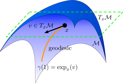
Figure 1: Exponential map on $\mathcal{M}$.

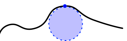
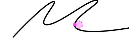
Figure 2: Manifolds with large and small reach.

2.2 Optimal Transport Theory

Let $\mu,\nu$ be absolutely continuous measures on sets $X,Y\subseteq\mathbb{R}^{d}$. We say a function $f:X\to Y$ transports $\mu$ onto $\nu$ if $f_{\sharp}\mu=\nu$. In words, for all measurable sets $A$ we have

$$\nu(A)=f_{\sharp}\mu(A)=\mu\left(f^{-1}(A)\right),$$

where $f^{-1}(A)$ is the pre-image of $A$ under $f$. Optimal transport studies the maps taking source measures $\mu$ on $X$ to target measures $\nu$ on $Y$ which also minimize a cost $c:X\times Y\to\mathbb{R}_{\geq 0}$ among all such transport maps. However the results are largely restricted to transport between measures on the same dimensional Euclidean space. In this paper, we will make use of the main theorem in Caffarelli (1992), in the form presented in Villani (2008).

Proposition 1.

Let $c(x,y)=\|x-y\|^{2}$ in $\mathbb{R}^{d}\times\mathbb{R}^{d}$ and let $\Omega_{1},\Omega_{2}$ be nonempty, connected, bounded, open subsets of $\mathbb{R}^{d}$. Let $f_{1},f_{2}$ be probability densities on $\Omega_{1}$ and $\Omega_{2}$ respectively, with $f_{1},f_{2}$ bounded from above and below. Assume further that $\Omega_{2}$ is convex. Then there exists a unique optimal transport map $T:\Omega_{1}\rightarrow\Omega_{2}$ for the associated probability measures $\mu(dx)=f_{1}(x)\,dx$ and $\nu(dy)=f_{2}(y)\,dy$, and the cost $c$. Furthermore, we have that $T\in C^{\alpha}(\Omega_{1})$ for some $\alpha\in(0,1)$.

This proposition allows to produce Hölder transport maps which can be further approximated with neural networks with size depending on a given accuracy.

To connect optimal transport and Riemannian manifolds, we first define the volume measure on a manifold $\mathcal{M}$ and establish integration on $\mathcal{M}$.

Definition 4 (Volume measure).

Let $\mathcal{M}$ be a compact $d$-dimensional Riemannian manifold. We define the volume measure $\mu_{\mathcal{M}}$ on $\mathcal{M}$ as the restriction of the $d$-dimensional Hausdorff measure $\mathcal{H}^{d}$.

A definition for the restriction of the Hausdorff measure can be found in Federer (1959).

We say that the distribution $Q$ has density $q$ if the Radon-Nikodym derivative of $Q$ with respect to $\mu_{\mathcal{M}}$ is $q$. According to Evans and Gariepy (1992)), for any continuous function $f:\mathcal{M}\to\mathbb{R}$ supported within the image of the ball $B_{T_{x}\mathcal{M}}(0,\epsilon)$ under the exponential map for $\epsilon<\text{inj}(\mathcal{M})$, we have

$$\int f\,dQ=\int(fq)\,d\mu_{\mathcal{M}}=\int_{B_{T_{x}\mathcal{M}}(0,\epsilon)}(fq)\circ\exp_{x}(v)\sqrt{\det g_{ij}^{x}(v)}\,dv.$$ (5)

Here $g_{ij}^{x}(v)=\langle\partial\exp_{x}(v)[e_{i}],\partial\exp_{x}(v)[e_{j}]\rangle$ with $(e_{1},...,e_{d})$ an orthonormal basis of $T_{x}\mathcal{M}$.

3 Main Results

We will present our main results in this section, including an approximation theory for a large class of distributions on a Riemannian manifold (Theorem 1), and a statistical estimation theory of deep generative networks for distribution learning (Theorem 2).

We make some regularity assumptions on a manifold $\mathcal{M}$ and assume the target data distribution $Q$ is supported on $\mathcal{M}$. The easy-to-sample distribution $\rho$ is taken to be uniform on $(0,1)^{d+1}$.

Assumption 1.

$\mathcal{M}$ is a $d$-dimensional compact Riemannian manifold isometrically embedded in ambient dimension $\mathbb{R}^{D}$. Via compactness, $\mathcal{M}$ is bounded: there exists $M>0$ such that $\|x\|_{\infty}\leq M$ , $\forall x\in\mathcal{M}$. Further suppose $\mathcal{M}$ has a positive reach $\tau>0$.

Assumption 2.

$Q$ is supported on $\mathcal{M}$ and has a density $q$ with respect to the volume measure on $\mathcal{M}$. Further we assume boundedness of $q$ i.e. there exists some constants $c,C>0$ such that $c\leq q\leq C$.

To justify the representation power of feedforward ReLU networks for learning the target distribution $Q$, we explicitly construct a neural network generator class, such that a neural network function in this generator class can pushfoward $\rho$ to a good approximation of $Q$.

Consider the following generator class $\mathcal{G}_{\textup{NN}}$

$$\mathcal{G}_{\textup{NN}}(L,p,\kappa)=\{ g=[g_{1},...,g_{D}]:\mathbb{R}^{d+1}\to\mathbb{R}^{D}|g_{j}\textup{ in form }(\ref{nnform})\text{ with at most }L\textup{ layers}$$

$$\textup{ and max width }p,\text{ while }\left\lvert\left\lvert W_{i}\right\rvert\right\rvert_{\infty}\leq\kappa,\left\lvert\left\lvert b_{i}\right\rvert\right\rvert_{\infty}\leq\kappa\textup{ for all }i\in[L],j\in[D]\},$$

where $\|\cdot\|_{\infty}$ is the maximum magnitude in a matrix or vector. The width of a neural network is the largest dimension (i.e. number of rows/columns) among the $W_{i}$’s and the $b_{i}$’s.

Theorem 1 (Approximation Power of Deep Generative Models).

Suppose $\mathcal{M}$ and $Q$ satisfy Assumptions 1 and 2 respectively. The easy-to-sample distribution $\rho$ is taken to be uniform on $(0,1)^{d+1}$. Then there exists a constant $0<\alpha<1$ (independent of $D$) such that for any $0<\epsilon<1$, there exists a $g_{\theta}\in\mathcal{G}_{\textup{NN}}(L,p,\kappa)$ with parameters

$$L= O\left(\log\left(\frac{1}{\epsilon}\right)\right),\hskip 7.22743ptp=O\left(D\epsilon^{-\frac{d}{\alpha}}\right),\hskip 7.22743pt\kappa=M$$

that satisfies

$$W_{1}((g_{\theta})_{\sharp}\rho,Q)<\epsilon.$$

Theorem 1 demonstrates the representation power of deep neural networks for distributions $Q$ on $\mathcal{M}$, which answers Question Q1. For a given accuracy $\epsilon$, there exists a neural network $g_{\theta}$ which pushes the uniform distribution on $(0,1)^{d+1}$ forward to a good approximation of $Q$ with accuracy $\epsilon$. The network size is exponential in the intrinsic dimension $d$. A proof sketch of Theorem 1 is given in Section 4.1.

We next present a statistical estimation theory to answer Question Q2.

Theorem 2 (Statistical Guarantees of Deep Wasserstein Learning).

Suppose $\mathcal{M}$ and $Q$ satisfy Assumption 1 and 2 respectively. The easy-to-sample distribution $\rho$ is taken to be uniform on $(0,1)^{d+1}$. Let $n$ be the number of samples of $X_{i}\sim Q$. Choose any $\delta>0$. Set $\epsilon=n^{-\frac{1}{d+\delta}}$ in Theorem 1 so that the network class $\mathcal{G}_{\textup{NN}}(L,p,\kappa)$ has parameters

$$L= O\left(\log\left(n^{\frac{1}{d+\delta}}\right)\right),\hskip 7.22743ptp=O\left(Dn^{\frac{d}{\alpha(d+\delta)}}\right),\hskip 7.22743pt\kappa=M.$$

Then the empirical risk minimizer $\hat{g}_{n}$ given by (4) has rate

$$\mathbb{E}W_{1}((\hat{g}_{n})_{\sharp}\rho,Q)\leq Cn^{-\frac{1}{d+\delta}},$$

where $C$ is a constant independent of $n$ and $D$.

A proof sketch of Theorem 2 is presented in Section 4.2. Additionally, this result can be easily extended to the noisy case. Suppose we are given $n$ noisy i.i.d. samples $\hat{X}_{1},...,\hat{X}_{n}$ of the form $\hat{X}_{i}=X_{i}+\xi_{i}$, for $X_{i}\sim Q$ and $\xi_{i}$ distributed according to some noise distribution. The optimization in (4) is performed with the noisy empirical distribution $\hat{Q}_{n}=\frac{1}{n}\sum_{i=1}^{n}\delta_{\hat{X}_{i}}$. Then the minimizer $\hat{g}_{n}$ satisfies

$$\mathbb{E}W_{1}((\hat{g}_{n})_{\sharp}\rho,Q)\leq Cn^{-\frac{1}{d+\delta}}+2\sqrt{V_{\xi}},$$

where $V_{\xi}=\mathbb{E}\|\xi\|_{2}^{2}$ is the variance of the noise distribution. The proof in the noisy case is given in Section 4.3.

Comparison to Related Works. To justify the practical power of generative networks, low-dimensional data structures are considered in Luise et al. (2020); Schreuder et al. (2021); Block et al. (2021); Chae et al. (2021). These works consider the generative models in (1). They assume that the high-dimensional data are parametrized by low-dimensional latent parameters. Such assumptions correspond to the manifold model where the manifold is globally homeomorphic to Euclidean space, i.e. the manifold has a single chart.

In Luise et al. (2020), the generative models are assumed to be continuously differentiable up to order $s$. By jointly training of the generator and the latent distributions, they proved that the Sinkhorn divergence between the generated distribution and data distribution converges, depending on data intrinsic dimension. Chae et al. (2021) and Schreuder et al. (2021) assume the special case where the manifold has a single chart. More recently, Block et al. (2021) proposed to estimate the intrinsic dimension of data using the Hölder IPM between some empirical distributions of data. This theory is based on the statistical convergence of the empirical distribution to the data distribution. As an application to GANs, (Block et al., 2021, Theorem 23) gives the statistical error while the approximation error is not studied. In these works, the single chart assumption is very strong while a general manifold can have multiple charts.

Recently, Yang et al. (2022); Huang et al. (2022) showed that GANs can approximate any data distribution (in any dimension) by transforming an absolutely continuous 1D distribution. The analysis in Yang et al. (2022); Huang et al. (2022) can be applied to the general manifold model. Their approach requires the GAN to memorize the empirical data distribution using ReLU networks. Thus it is not clear how the designed generator is capable of generating new samples that are different from the training data. In contrast, we explicitly construct an oracle transport map which transforms the low-dimensional easy-to-sample distribution to the data distribution. Our work provides insights about how distributions on a manifold can be approximated by a neural network pushforward of a low-dimensional easy-to-sample distribution without exactly memorizing the data. In comparison, the single-chart assumption in earlier works assumes that an oracle transport naturally exists. Our work is novel in the construction of the oracle transport for a general manifold with multiple charts, and the approximation theory by deep neural networks.

4 Proof of Main Results

4.1 Proof of Approximation Theory in Theorem 1

To prove Theorem 1, we explicitly construct an oracle transport $g^{*}$ pushing $\rho$ onto $Q$, i.e. $g^{*}_{\sharp}\rho=Q$. Further this oracle will be piecewise $\alpha$-Hölder continuous for some $\alpha\in(0,1)$.

Lemma 1.

Suppose $\mathcal{M}$ and $Q$ satisfy Assumption 1 and 2 respectively. The easy-to-sample distribution $\rho$ is taken to be uniform on $(0,1)^{d+1}$. Then there exists a function $g^{*}:(0,1)^{d+1}\to\mathcal{M}$ such that $Q=g^{*}_{\sharp}\rho$ where

$$g^{*}(x)=\textstyle\sum_{j=1}^{J}\mathds{1}_{(\pi_{j-1},\pi_{j})}(x_{1})g^{*}_{j}(x_{2:d+1})$$ (6)

for some $\alpha$-Hölder ($0<\alpha<1$) continuous functions $g_{1}^{*},\dots,g_{J}^{*}$ and some constants $0=\pi_{0}<\pi_{1}<\dots<\pi_{J}=1$.

Proof.

We construct a transport map $g^{*}:(0,1)^{d+1}\to\mathcal{M}$ that can be approximated by neural networks. First, we decompose the manifold into overlapping geodesic balls. Next, we pull these local distributions on these balls back to tangent space, which produces $d$-dimensional tangent distributions. Then, we apply optimal theory on these tangent distributions to produce maps between the source distributions on $(0,1)^{d}$ to the appropriate local (geodesic ball) distributions on the manifold. Finally, we glue together these local maps with indicators functions and a uniform random sample from $(0,1)$. We proceed with the first step of decomposing the manifold.

Step 1: Overlapping ball decomposition. Recall that $\mathcal{M}$ is a compact manifold with reach $\tau>0$. Then the injectivity radius of $\mathcal{M}$ is greater or equal to $\pi\tau$ (Aamari et al. (2019)). Set $r=\frac{\pi\tau}{2}$. For each $c\in\mathcal{M}$, define an open set $U_{c}=\exp_{c}(B_{T_{c}\mathcal{M}}(0,r))\subseteq\mathcal{M}$. Since the collection $\{U_{c}:x\in\mathcal{M}\}$ forms an open cover of $\mathcal{M}$ (in $\mathbb{R}^{D}$), by the compactness of $\mathcal{M}$ we can extract a finite subcover which we denote as $\{U_{c_{j}}\}_{j=1}^{J}$. For convenience, we will write $U_{j}=U_{c_{j}}$.

Step 2: Defining local lower-dimensional distributions. On each $U_{j}$, we define a local distribution $Q_{j}$ with density $q_{j}$ via

$$q_{j}(x)=\frac{q(x)}{Q(U_{j})}\mathds{1}_{U_{j}}(x).$$

Set $K(x)=\sum_{j=1}^{J}\mathds{1}_{U_{j}}(x)$ as the number of balls $U_{j}$ containing $x$. Note $1\leq K(x)\leq J$ for all $x\in\mathcal{M}$. Now define the distribution $\overline{Q}_{j}$ with density $\overline{q}_{j}$ given by

$$\overline{q}_{j}(x)=\frac{\frac{1}{K(x)}q_{j}(x)\mathds{1}_{U_{j}}(x)}{\int_{U_{j}}\frac{1}{K(x)}q_{j}(x)d\mathcal{H}}.$$

Write $K_{j}=\int_{U_{j}}\frac{1}{K(x)}q_{j}(x)d\mathcal{H}$ as the normalizing constant. Define $\tilde{q}_{j}(v)=(\overline{q}_{j}\circ\exp_{c_{j}})(v)\sqrt{\det g_{kl}^{c_{j}}(v)}$ where $g_{kl}^{c_{j}}$ is the Riemannian at $c_{j}$. This quantity can be thought of as the Jacobian of the exponential map, denoted by $|J_{\exp_{c_{j}}}(v)|$ in the following step. Then $\tilde{q}_{j}$ is a density on $\tilde{U}_{j}=\exp^{-1}_{c_{j}}(U_{j})$, which is a ball of radius $\frac{\pi\tau}{2}$ since

$$1=\int_{U_{j}}\overline{q}_{j}(x)d\mathcal{H}=\int_{\tilde{U}_{j}}\sqrt{\det g_{kl}^{c_{j}}(v)}\overline{q}_{j}(\exp_{c_{j}}(v))dv=\int_{\tilde{U}_{j}}\tilde{q}_{j}(v)dv$$

Let $\tilde{Q}_{j}$ be the distribution in $\mathbb{R}^{d}$ with density $\tilde{q}_{j}$. By construction, we can write

$$\overline{Q}_{j}=(\exp_{c_{j}})_{\sharp}\tilde{Q}_{j}.$$ (7)

Step 3: Constructing the local transport. We have that $\exp_{c_{j}}^{-1}$ is bi-Lipschitz on $U_{j}$ and hence its Jacobian is upper bounded. Since $|J_{\exp_{c_{j}}}(v)|=\frac{1}{|J_{\exp_{c_{j}}^{-1}}(x)|}$, we know that $|J_{\exp_{c_{j}}}|$ lower bounded. Since $q_{j}$ is lower bounded (away from $0$), this means $\tilde{q}_{j}$ is also lower bounded. Now the distribution $\tilde{\rho}_{j}$ supported on $\tilde{U}_{j}=B(0,\frac{\tau\pi}{2})$ fulfills the requirements for our optimal transport result: (1) Its density $\tilde{p}_{j}$ is lower and upper bounded; (2) The support $B(0,\frac{\tau\pi}{2})$ is convex. Taking our cost to be $c(x,y)=\frac{1}{2}\|x-y\|^{2}$ (i.e. squared Euclidean distance), via Proposition 1 we can find an optimal transport map $T_{j}$ such that

$$(T_{j})_{\sharp}\rho_{d}=\tilde{Q}_{j}$$ (8)

where $\rho_{d}$ is uniformly distributed on $(0,1)^{d}$. Furthermore, $T_{j}\in C^{\alpha_{j}}$ for some $\alpha_{j}\in(0,1)$. Then we can construct a local transport onto $U_{j}$ via

$$g_{j}^{*}=\exp_{c_{j}}\circ T_{j}$$ (9)

which pushes $\rho_{d}$ forward to $\overline{Q}_{j}$. Since $g_{j}^{*}$ is a composition of a Lipschitz map with an $\alpha_{j}$ Hölder continuous maps, it is hence $\alpha_{j}$ Hölder continuous.

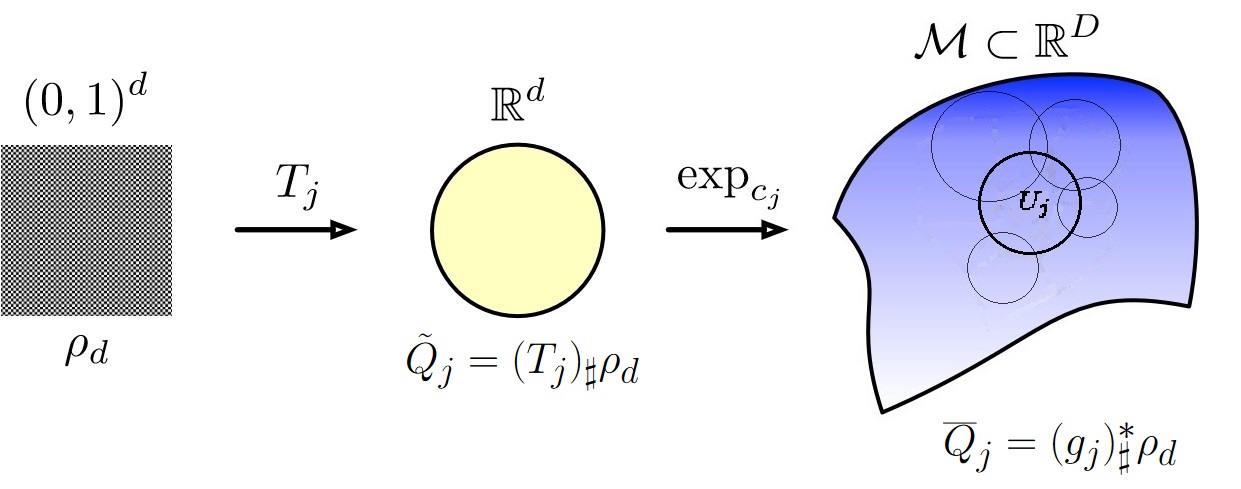
Figure 3: Local transport $g_{j}^{*}$ in (9) mapping $\rho_{d}$ on $(0,1)^{d}$ to a local distribution $\overline{Q}_{j}$ supported on $U_{j}$.

Step 4: Assembling the global transport. It remains to patch together the local distributions $\overline{Q}_{j}$ to form $Q$. Define $\eta_{j}=K_{j}Q(U_{j})$. Notice

$$\sum_{j=1}^{J}\eta_{j}\overline{q}_{j}(x) =\sum_{j=1}^{J}K_{j}Q(U_{j})\frac{\frac{1}{K(x)}q_{j}(x)\mathds{1}_{U_{j}}(x)}{K_{j}}=\sum_{j=1}^{J}Q(U_{j})\frac{\frac{1}{K(x)}q(x)\mathds{1}_{U_{j}}(x)}{Q(U_{j})}$$

$$=\sum_{j=1}^{J}\frac{1}{K(x)}q(x)\mathds{1}_{U_{j}}(x)=q(x)\frac{1}{K(x)}\sum_{j=1}^{J}\mathds{1}_{U_{j}}(x)=q(x).$$

Hence it must be that $\sum_{j=1}^{J}\eta_{j}=1$. Set $\alpha=\min_{j\in[J]}\alpha_{j}$. We can now define the oracle $g^{*}$. Let $x\in(0,1)^{d+1}$. Write

$$g^{*}(x)=\textstyle\sum_{j=1}^{J}\mathds{1}_{(\pi_{j-1},\pi_{j})}(x_{1})g_{j}^{*}(x_{2:d+1}),$$ (10)

where $x_{1}$ is the first coordinate and $x_{2:d+1}$ are the remaining coordinates with $\pi_{j}=\sum_{i=1}^{j-1}\eta_{i}$. Let $Z\sim\rho$. Then $g(Z)\sim Q$. We see this as follows. For $A\subseteq\mathcal{M}$ we can compute

$$\mathbb{P}(g^{*}(Z)\in A) =\sum_{j=1}^{J}\mathbb{P}(\pi_{j-1}<Z_{1}<\pi_{j})\mathbb{P}(g^{*}_{j}(Z_{2:d+1})\in A\cap U_{j})=\sum_{j=1}^{J}\eta_{j}\overline{Q}_{j}(A\cap U_{j})$$

$$=\sum_{j=1}^{J}\eta_{j}\int_{A}\overline{q}_{j}(x)d\mathcal{H}=\int_{A}\sum_{j=1}^{J}\eta_{j}\overline{q}_{j}(x)d\mathcal{H}=\int_{A}q(x)d\mathcal{H}=Q(A)$$

which completes the proof. ∎

We have found an oracle $g^{*}$ which is piecewise Hölder continuous such that $g^{*}_{\sharp}\rho=Q$. We can design a neural network $g_{\theta}$ to approximate this oracle $g^{*}$. Now in order to minimize $W_{1}((g_{\theta})_{\sharp}\rho,Q)=W_{1}((g_{\theta})_{\sharp}\rho,g^{*}_{\sharp}\rho)$, we show it suffices to have $g_{\theta}$ approximate $g^{*}$ in $L^{1}(\rho)$.

Lemma 2.

Let $\mu$ be an absolutely continuous probability distribution on a set $Z\subseteq\mathbb{R}^{d}$, and let $f,g:Z\rightarrow\mathbb{R}^{m}$ be transport maps. Then

$$W_{1}(f_{\sharp}\mu,g_{\sharp}\mu)\leq C\|f-g\|_{L^{1}(\mu)}$$

for some $C>0$.

Proof of Lemma 2.

The vector-valued functions $f$ and $g$ output $m$-dimensional vectors. Note that $||f-g||_{L^{1}(\mu)}=\sum_{i=1}^{m}\|f_{i}-g_{i}\|$ where $f_{i}$ and $g_{i}$ denote the $i$th component function of $f$ and $g$, respectively. Then we can compute

$$W_{1}(f_{\sharp}\mu,g_{\sharp}\mu) =\sup_{\phi\in\text{Lip}_{1}(\mathbb{R}^{m})}\left|\int\phi(y)\,d(f_{\sharp}\mu)-\int\phi(y)\,d(g_{\sharp}\mu)\right|$$

$$=\sup_{\phi\in\text{Lip}_{1}(\mathbb{R}^{m})}\left|\int\phi(f(x))-\phi(g(x))\,d\mu\right|$$

$$\leq\sup_{\phi\in\text{Lip}_{1}(\mathbb{R}^{m})}\int\left|\phi(f(x))-\phi(g(x))\right|\,d\mu$$

$$\leq\int_{Z}\left\|f(x)-g(x)\right\|_{2}\,d\mu$$

$$\leq\int_{Z}C\|f(x)-g(x)\|_{1}\,d\mu$$

$$=C\|f-g\|_{L^{1}(\mu)},$$

since $\phi$ is Lipschitz with constant $1$ and all norms are equivalent in finite dimensions. In particular, $C=1$ here.

∎

We now prove Theorem 1.

Proof of Theorem 1.

By Lemma 1, there exists a transformation $g^{*}(x)=\sum_{j=1}^{J}\mathds{1}_{(\pi_{j-1},\pi_{j})}(x_{1})g^{*}_{j}(x_{2:d+1})$ such that $g^{*}_{\sharp}\rho=Q$. By Lemma 2, it suffices to approximate $g^{*}$ with a neural network $g_{\theta}\in\mathcal{G}_{\textup{NN}}(L,p,\kappa)$ in $L^{1}$ norm, with a given accuracy $\epsilon>0$. Let $(g^{*})^{(i)}$ denote the $i$th component of the vector valued function $g^{*}$. Then it suffices to approximate

$$(g^{*})^{(i)}(x)=\sum_{j=1}^{J}\mathds{1}_{(\pi_{j-1},\pi_{j})}(x_{1})(g^{*}_{j})^{(i)}(x_{2:d+1})$$

for each $1\leq i\leq D$, where $(g^{*}_{j})^{(i)}$ denotes the $i$th component of the function $g^{*}_{j}$. We construct the approximation of $(g^{*})^{(i)}$ by the function

$$(g_{\theta})^{(i)}(x)=\sum_{j=1}^{J}\tilde{\times}^{\delta_{2}}\left(\tilde{\mathds{1}}^{\delta_{1}}_{(\pi_{j-1},\pi_{j})}(x_{1}),(g_{j,\theta}^{\delta_{3}})^{(i)}(x_{2:d+1})\right),$$ (11)

where $\tilde{\times}^{\delta_{2}}$ is a ReLU network approximation to the multiplication operation with $\delta_{2}$ accuracy, $\tilde{\mathds{1}}^{\delta_{1}}_{(\pi_{j-1},\pi_{j})}$ is a ReLU network approximation to the indicator function with $\delta_{1}$ accuracy, and $(g_{j,\theta}^{\delta_{3}})^{(i)}$ is a ReLU network approximation to $(g_{j}^{*})^{(i)}$ with $\delta_{3}$ accuracy. We construct these using the approximation theory outlined in Appendix A.

First, we obtain $\tilde{\mathds{1}}^{\delta_{1}}_{(\pi_{j-1},\pi_{j})}$ via an application of Lemma 11. Next, we obtain $\tilde{\times}^{\delta_{2}}$ from an application of Lemma 9. Finally, we discuss $g_{j,\theta}^{\delta_{3}}$. Let $j\in[J]$. To approximate the Hölder function $g_{j}^{*}$, we use the following Lemma 3 that is proved in Appendix A. Similar approximation results can be found in Shen et al. (2022) and Ohn and Kim (2019) as well. In Lemma 3, our approximation error is in $L^{1}$ norm and all weight parameters are upper bounded by a constant. In comparison, the error in Ohn and Kim (2019) is in $L^{\infty}$ norm and the weight parameter increases as $\epsilon$ decreases.

Lemma 3.

Fix $M\geq 2$. Suppose $f\in C^{\alpha}([0,1]^{d})$, $\alpha\in(0,1]$, with $\|f\|_{L^{\infty}}<M$. Let $0<\epsilon<1$. Then there exists a function $\Phi$ implementable by a ReLU network such that

$$\|f-\Phi\|_{L^{1}}<\epsilon.$$

The ReLU network has depth at most $c_{1}\log\left(\frac{1}{\epsilon}\right)$, width at most $c_{2}\epsilon^{-\frac{d}{\alpha}}$, and weights bounded by $M$ (where $c_{1}$ and $c_{2}$ are constants independent of $\epsilon$).

We can apply Lemma 3 to $(g_{j}^{*})^{(i)}$ for all $1\leq j\leq J$ and $1\leq i\leq D$, since they are all elements of $C^{\alpha}(0,1)^{d}$ and elements of $C^{\alpha}(0,1)^{d}$ can be extended to $C^{\alpha}[0,1]^{d}$. Thus there exists a neural network $(g_{j,\theta}^{\delta_{3}})^{(i)}\in\mathcal{G}_{\textup{NN}}(L,p,\kappa)$ with parameters given as above such that

$$\|(g_{j}^{*})^{(i)}-(g_{j,\theta}^{\delta_{3}})^{(i)}\|_{L^{1}}<\delta_{3}.$$

The goal is now to show the $L^{1}$ distance between $g_{\theta}$ (as defined in (11)) and $g^{*}$ is small. We compute

$$\quad\|g^{*}-g_{\theta}\|_{L^{1}}$$

$$=\sum_{i=1}^{D}\|(g^{*})^{(i)}-(g_{\theta})^{(i)}\|_{L^{1}}$$

$$=\sum_{i=1}^{D}\int_{(0,1)^{d+1}}\left|(g^{*})^{(i)}(x)-(g_{\theta})^{(i)}(x)\right|\,dx$$

$$\leq\sum_{i=1}^{D}\sum_{j=1}^{J}\int_{(0,1)^{d+1}}\left|\tilde{\times}^{\delta_{2}}\left(\tilde{\mathds{1}}^{\delta_{1}}_{(\pi_{j-1},\pi_{j})}(x_{1}),(g_{j,\theta}^{\delta_{3}})^{(i)}(x_{2:d+1})\right)-\mathds{1}_{(\pi_{j-1},\pi_{j})}(x_{1})(g^{*}_{j})^{(i)}(x_{2:d+1})\right|\,dx$$

$$\leq\sum_{i=1}^{D}\sum_{j=1}^{J}\int_{(0,1)^{d+1}}\left|\tilde{\times}^{\delta_{2}}\left(\tilde{\mathds{1}}^{\delta_{1}}_{(\pi_{j-1},\pi_{j})}(x_{1}),(g_{j,\theta}^{\delta_{3}})^{(i)}(x_{2:d+1})\right)-\tilde{\mathds{1}}^{\delta_{1}}_{(\pi_{j-1},\pi_{j})}(x_{1})(g_{j,\theta}^{\delta_{3}})^{(i)}(x_{2:d+1})\right|\,dx$$

$$\quad+\sum_{i=1}^{D}\sum_{j=1}^{J}\int_{(0,1)^{d+1}}\left|\tilde{\mathds{1}}^{\delta_{1}}_{(\pi_{j-1},\pi_{j})}(x_{1})(g_{j,\theta}^{\delta_{3}})^{(i)}(x_{2:d+1})-\mathds{1}_{(\pi_{j-1},\pi_{j})}(x_{1})(g_{j,\theta}^{\delta_{3}})^{(i)}(x_{2:d+1})\right|\,dx$$

$$\quad+\sum_{i=1}^{D}\sum_{j=1}^{J}\int_{(0,1)^{d+1}}\left|\mathds{1}_{(\pi_{j-1},\pi_{j})}(x_{1})(g_{j,\theta}^{\delta_{3}})^{(i)}(x_{2:d+1})-\mathds{1}_{(\pi_{j-1},\pi_{j})}(x_{1})(g_{j}^{*})^{(i)}(x_{2:d+1})\right|\,dx$$

$$=\sum_{i=1}^{D}\sum_{j=1}^{J}\left(\text{(I) + (II) + (III)}\right)$$

Each of the three terms are easily handled as follows.

1. By construction of $\tilde{\times}^{\delta_{2}}$ in Lemma 9, we have that

   (I) $$=\int_{(0,1)^{d+1}}\left|\tilde{\times}^{\delta_{2}}\left(\tilde{\mathds{1}}^{\delta_{1}}_{(\pi_{j-1},\pi_{j})}(x_{1}),(g_{j,\theta}^{\delta_{3}})^{(i)}(x_{2:d+1})\right)-\tilde{\mathds{1}}^{\delta_{1}}_{(\pi_{j-1},\pi_{j})}(x_{1})(g_{j,\theta}^{\delta_{3}})^{(i)}(x_{2:d+1})\right|\,dx$$

   $$\leq\int_{(0,1)^{d+1}}\delta_{2}\,dx=\delta_{2}.$$

2. By construction of $\tilde{\mathds{1}}^{\delta_{1}}_{(\pi_{j-1},\pi_{j})}$ in Lemma 11, we have that

   (II) $$=\int_{(0,1)^{d+1}}\left|\tilde{\mathds{1}}^{\delta_{1}}_{(\pi_{j-1},\pi_{j})}(x_{1})(g_{j,\theta}^{\delta_{3}})^{(i)}(x_{2:d+1})-\mathds{1}_{(\pi_{j-1},\pi_{j})}(x_{1})(g_{j,\theta}^{\delta_{3}})^{(i)}(x_{2:d+1})\right|\,dx$$

   $$\leq\left\|(g_{j,\theta}^{\delta_{3}})^{(i)}\right\|_{\infty}\int_{0}^{1}\left|\tilde{\mathds{1}}^{\delta_{1}}_{(\pi_{j-1},\pi_{j})}(x_{1})-\mathds{1}_{(\pi_{j-1},\pi_{j})}(x_{1})\right|\,dx$$

   $$\leq M\left\|\tilde{\mathds{1}}^{\delta_{1}}_{(a,b)}-\mathds{1}_{(a,b)}\right\|_{L^{1}}$$

   $$=M\delta_{1}.$$

3. By construction of $(g_{j,\theta}^{\delta_{3}})^{(i)}$ from Lemma 3, we have that

   (III) $$=\int_{(0,1)^{d+1}}\left|\mathds{1}_{(\pi_{j-1},\pi_{j})}(x_{1})(g_{j,\theta}^{\delta_{3}})^{(i)}(x_{2:d+1})-\mathds{1}_{(\pi_{j-1},\pi_{j})}(x_{1})(g_{j}^{*})^{(i)}(x_{2:d+1})\right|\,dx$$

   $$=\|\mathds{1}_{(\pi_{j-1},\pi_{j})}\|_{\infty}\int_{(0,1)^{d}}\left|(g_{j,\theta}^{\delta_{3}})^{(i)}(x)-(g_{j}^{*})^{(i)}(x)\right|\,dx$$

   $$=\left\|(g_{j,\theta}^{\delta_{3}})^{(i)}-(g_{j}^{*})^{(i)}\right\|_{L^{1}}$$

   $$\leq\delta_{3}.$$

As a result, we have that

$$\|g^{*}-g_{\theta}\|_{L^{1}}\leq\sum_{i=1}^{D}\sum_{j=1}^{J}\text{(I)}+\text{(II)}+\text{(III)}\leq\sum_{i=1}^{D}\sum_{j=1}^{J}\delta_{2}+M\delta_{1}+\delta_{3}=DJ(M\delta_{1}+\delta_{2}+\delta_{3}).$$

By selecting $\delta_{1}<\frac{\epsilon}{3DJM}$, $\delta_{2}<\frac{\epsilon}{3DJ}$, and $\delta_{3}<\frac{\epsilon}{3DJ}$, we obtain that $||g^{*}-g_{\theta}||_{1}<\epsilon$.

To complete the proof, we note that $g_{\theta}$ can be exactly represented by a neural network in $\mathcal{G}_{\textup{NN}}(L,p,\kappa)$ with parameters

$$L= O\left(\log\left(\frac{1}{\epsilon}\right)\right),\hskip 7.22743ptp=O\left(D\epsilon^{-\frac{d}{\alpha}}\right),\hskip 7.22743pt\kappa=M.$$

∎

4.2 Proof of Statistical Estimation Theory in Theorem 2

The proof of Theorem 2 is facilitated by the common bias-variance inequality, presented here as a lemma.

Lemma 4.

Under the same assumptions of Theorem 2, we have

$$\mathbb{E}W_{1}((\hat{g}_{n})_{\sharp}\rho,Q)\leq\inf_{g_{\theta}\in\mathcal{G}_{\textup{NN}}}W_{1}((g_{\theta})_{\sharp}\rho,Q)+2\mathbb{E}W_{1}(Q_{n},Q)$$ (12)

where $Q_{n}$ is the clean empirical distribution.

Proof.

Recalling the definition of $\hat{g}_{n}$ as the empirical risk minimizer, we compute

$$\mathbb{E}W_{1}((\hat{g}_{n})_{\sharp}\rho,Q) \leq\mathbb{E}W_{1}((\hat{g}_{n})_{\sharp}\rho,Q_{n})+\mathbb{E}W_{1}(Q_{n},Q)$$

$$=\mathbb{E}\inf_{g_{\theta}\in\mathcal{G}_{\textup{NN}}}W_{1}((g_{\theta})_{\sharp}\rho,Q_{n})+\mathbb{E}W_{1}(Q_{n},Q)$$

$$\leq\mathbb{E}\inf_{g_{\theta}\in\mathcal{G}_{\textup{NN}}}W_{1}((g_{\theta})_{\sharp}\rho,Q)+2\mathbb{E}W_{1}(Q_{n},Q)$$

since $W_{1}((\hat{g}_{n})_{\sharp}\rho,Q_{n})=\inf_{g_{\theta}\in\mathcal{G}_{\rm NN}}W_{1}((g_{\theta})_{\sharp}\rho,Q_{n})$ from (4).

∎

In the right hand side of (12), the first term is the approximation error and the second term is the statistical error. This naturally decomposes the problem into two parts: one controlling the approximation error and the other controlling the statistical error. The bias term can be controlled via Theorem 1. To control convergence of the empirical distribution $Q_{n}$ to $Q$ we leverage the existing theory (Weed and Bach, 2019) to obtain the following lemma.

Lemma 5.

Under the same assumptions of Theorem 2, for all $\delta>0$, $\exists C_{\delta}>0$ such that

$$\mathbb{E}\left[W_{1}(Q,Q_{n})\right]\leq C_{\delta}n^{-\frac{1}{d+\delta}}.$$ (13)

Proof of Lemma 5.

Let $\delta>0$. Consider the manifold $\mathcal{M}$ with the geodesic distance as a metric space. When (Weed and Bach, 2019, Theorem 1) is applied to $\mathcal{M}$ with the geodesic distance, we have that

$$\mathbb{E}\left[W^{\mathcal{M}}_{1}(Q,Q_{n})\right]\leq C_{\delta}n^{-\frac{1}{d+\delta}}$$

for some constant $C_{\delta}$ independent of $n$. Here, $W^{\mathcal{M}}_{1}$ is the $1$-Wasserstein distance on $\mathcal{M}$ with the geodesic distance. It suffices to show that

$$W_{1}^{\mathbb{R}^{D}}(Q,Q_{n})=W_{1}(Q,Q_{n})\leq W_{1}^{\mathcal{M}}(Q,Q_{n}).$$

Let $\text{Lip}_{1}(\mathbb{R}^{D})$ and $\text{Lip}_{1}(\mathcal{M})$ denote the set of $1$-Lipschitz functions defined on $\mathcal{M}$ with respect to the Euclidean distance on $\mathbb{R}^{D}$ and geodesic distance on $\mathcal{M}$ respectively. But note that $\text{Lip}_{1}(\mathbb{R}^{D})\subseteq\text{Lip}_{1}(\mathcal{M})$ because for any $f\in\text{Lip}_{1}(\mathbb{R}^{D})$ we have

$$\frac{|f(x)-f(y)|}{\|x-y\|_{\mathcal{M}}}\leq\frac{|f(x)-f(y)|}{\|x-y\|_{\mathbb{R}^{D}}}\leq 1$$

as $\|x-y\|_{\mathbb{R}^{D}}\leq\|x-y\|_{\mathcal{M}}$ under an isometric embedding and hence $f\in\text{Lip}_{1}(\mathcal{M})$. Thus

$$\mathbb{E}\left[W_{1}(Q,Q_{n})\right]\leq\mathbb{E}\left[W_{1}^{\mathcal{M}}(Q,Q_{n})\right]\leq C_{\delta}n^{-\frac{1}{d+\delta}}.$$

∎

Finally, we prove our statistical estimation result in Theorem 2.

Proof of Theorem 2.

Choose $\delta>0$. Recall from Lemma 4 we have

$$W_{1}((\hat{g}_{n})_{\sharp}\rho,Q)\leq\mathbb{E}\inf_{g_{\theta}\in\mathcal{G}_{\textup{NN}}}W_{1}((g_{\theta})_{\sharp}\rho,Q)+2\mathbb{E}W_{1}(Q_{n},Q)$$

The first term is the approximation error which can be controlled within an arbitrarily small accuracy $\epsilon$. Theorem 1 shows the existence of a neural network function $g_{\theta}$ with $O\left(\log\left(\frac{1}{\epsilon}\right)\right)$ layers and $O(D\epsilon^{-d/\alpha}\log(\frac{1}{\epsilon}))$ neurons such that $W_{1}((g_{\theta})_{\sharp}\rho,Q)\leq\epsilon$ for any $\epsilon>0$. We choose $\epsilon=n^{-\frac{1}{d+\delta}}$ to optimally balance the approximation error and the statistical error. The second term is the statistical error for which we recall from Lemma 5 that $\mathbb{E}\left[W_{1}(\hat{Q}_{n},Q)\right]\leq C_{\delta}n^{-\frac{1}{d+\delta}}$ for some constant $C_{\delta}$.

Thus we have

$$\mathbb{E}W_{1}((\hat{g}_{n})_{\sharp}\rho,Q)\leq n^{-\frac{1}{d+\delta}}+2C_{\delta}n^{-\frac{1}{d+\delta}}=Cn^{-\frac{1}{d+\delta}}$$

by setting $C=1+2C_{\delta}$. This concludes the proof. ∎

4.3 Controlling the noisy samples

In the noisy setting, we are given $n$ noisy i.i.d. samples $\hat{X}_{1},...,\hat{X}_{n}$ of the form $\hat{X}_{i}=X_{i}+\xi_{i}$, for $X_{i}\sim Q$ and $\xi_{i}$ distributed according to some noise distribution. The optimization in (4) is performed with the noisy empirical distribution $\hat{Q}_{n}=\frac{1}{n}\sum_{i=1}^{n}\delta_{\hat{X}_{i}}$.

Lemma 6.

Under the same assumptions of Theorem 2 and in the noisy setting, we have

$$\mathbb{E}W_{1}((\hat{g}_{n})_{\sharp}\rho,Q)\leq\inf_{g_{\theta}\in\mathcal{G}_{\textup{NN}}}W_{1}((g_{\theta})_{\sharp}\rho,Q)+2\mathbb{E}W_{1}(Q_{n},Q)+2\mathbb{E}W_{1}(\hat{Q}_{n},Q_{n})$$ (14)

where $\hat{Q}_{n}$ is the noisy empirical distribution and $Q_{n}$ is the clean empirical distribution.

Proof.

Recalling the definition of $\hat{g}_{n}$ as the empirical risk minimizer, we compute

$$\mathbb{E}W_{1}((\hat{g}_{n})_{\sharp}\rho,Q) \leq\mathbb{E}W_{1}((\hat{g}_{n})_{\sharp}\rho,\hat{Q}_{n})+\mathbb{E}W_{1}(\hat{Q}_{n},Q)$$

$$\leq\mathbb{E}\inf_{g_{\theta}\in\mathcal{G}_{\textup{NN}}}W_{1}((g_{\theta})_{\sharp}\rho,\hat{Q}_{n})+\mathbb{E}W_{1}(Q_{n},Q)+\mathbb{E}W_{1}(\hat{Q}_{n},Q_{n})$$

$$\leq\mathbb{E}\inf_{g_{\theta}\in\mathcal{G}_{\textup{NN}}}W_{1}((g_{\theta})_{\sharp}\rho,Q)+2\mathbb{E}W_{1}(Q_{n},Q)+2\mathbb{E}W_{1}(\hat{Q}_{n},Q)$$

since $W_{1}((\hat{g}_{n})_{\sharp}\rho,\hat{Q}_{n})=\inf_{g_{\theta}\in\mathcal{G}_{\rm NN}}W_{1}((g_{\theta})_{\sharp}\rho,\hat{Q}_{n})$ from (4).

∎

Lemma 7.

Write $W_{1}(\hat{Q}_{n},Q_{n})=W_{1}^{\mathbb{R}^{D}}(\hat{Q}_{n},Q_{n})$. In the noisy setting, we express $\hat{X}_{i}=X_{i}+\xi_{i}$ where $X_{i}$ is drawn from $Q$ and then noised with $\xi_{i}$ drawn from some noise distribution. Then

$$\mathbb{E}[W_{1}(Q_{n},\hat{Q}_{n})]\leq\sqrt{V_{\xi}}$$

where $V_{\xi}=\mathbb{E}\|\xi\|_{2}^{2}$ which is the variance of the noise.

Proof.

Let $\hat{X}_{i},X_{i}$ be samples defining $\hat{Q}_{n},Q_{n}$ respectively. We have $\hat{X}_{i}=X_{i}+\xi_{i}$ where $\xi$ is the noise term. Compute

$$\mathbb{E}W_{1}(\hat{Q}_{n},Q_{n}) =\mathbb{E}\sup_{f\in\text{Lip}_{1}(\mathbb{R}^{D})}\hat{Q}_{n}(f)-Q_{n}(f)=\mathbb{E}\sup_{f\in\text{Lip}_{1}(\mathbb{R}^{D})}\frac{1}{n}\sum_{i=1}^{n}f(\hat{X}_{i})-f(X_{i})$$

$$\leq\mathbb{E}\sup_{f\in\text{Lip}_{1}(\mathbb{R}^{D})}\frac{1}{n}\sum_{i=1}^{n}|f(\hat{X}_{i})-f(X_{i})|=\mathbb{E}\sup_{f\in\text{Lip}_{1}(\mathbb{R}^{D})}\frac{1}{n}\sum_{i=1}^{n}|f(X_{i}+\xi_{i})-f(X_{i})|$$

$$\leq\mathbb{E}\sup_{f\in\text{Lip}_{1}(\mathbb{R}^{D})}\frac{1}{n}\sum_{i=1}^{n}\|\xi_{i}\|_{2}=\mathbb{E}\|\xi\|_{2}\leq\sqrt{V_{\xi}}$$

the last line follows from Jensen’s inequality. ∎

We conclude in the noisy setting that

$$\mathbb{E}W_{1}((\hat{g}_{n})_{\sharp}\rho,Q)\leq\epsilon_{\rm appx}+2C_{\delta}n^{-\frac{1}{d+\delta}}+2\sqrt{V}\leq Cn^{-\frac{1}{d+\delta}}+2\sqrt{V_{\xi}}$$

after balancing the approximation error $\epsilon_{\rm appx}$ appropriately.

5 Conclusion

We have established approximation and statistical estimation theories of deep generative models for estimating distributions on a low-dimensional manifold. The statistical convergence rate in this paper depends on the intrinsic dimension of data. In light of the manifold hypothesis, which suggests many natural datasets lie on low dimensional manifolds, our theory rigorously explains why deep generative models defy existing theoretical sample complexity estimates and the curse of dimensionality. In fact, deep generative models are able to learn low-dimensional geometric structures of data, and allow for highly efficient sample complexity independent of the ambient dimension. Meanwhile the size of the required network scales exponentially with the intrinsic dimension.

Our theory imposes very little assumption on the target density $Q$, requiring only that it admit a density $q$ with respect to the volume measure and that $q$ is upper and lower bounded. In particular we make no smoothness assumptions on $q$. This is practical, as we do not expect existing natural datasets to exhibit high degrees of smoothness.

In this work we assume access to computation of the $W_{1}$ distance. However during GAN training a discriminator is trained for this purpose. It would be of interest for future work to investigate the low-dimensional role of such discriminator networks which approximate the $W_{1}$ distance in practice.

Additionally, we provide an alternative approach to construct the oracle transport by decomposing the manifold into Voronoi cells and transporting the easy-to-sample distribution onto each disjoint cell directly in Appendix B.

Appendix A Deep ReLU Approximation of Hölder functions

In this section, $\log$ denotes the base 2 logarithm by default. $\bigtimes_{i=1}^{d}$ denotes the Cartesian product of $d$ sets. The goal is to determine the approximation rate of deep ReLU networks for Hölder continuous functions. Let $f\in C^{\alpha}([0,1]^{d})$ with Hölder norm $\|f\|_{C^{\alpha}}$ where $\alpha\in(0,1)$. We first approximate $f$ by a piecewise constant function $f^{n}$ in Section A.1, and then approximate $f^{n}$ by a deep ReLU Network $\Phi$ in Section A.3.

A.1 Piecewise constant approximation

Let $[n]^{d}=\{(a_{1},a_{2},\dots,a_{d}):a_{i}\in\mathbb{N},1\leq a_{i}\leq n\}$. Given any $n\in\mathbb{N}$, we cover $[0,1]^{d}$ by $n^{d}$ non-overlapping open cubes. For any $(k_{1},\dots,k_{d})=\vec{k}\in[n]^{d}$, we define

$$Q_{\vec{k}}=\bigtimes_{i=1}^{d}\left(\frac{k_{i}-1}{n},\frac{k_{i}}{n}\right).$$ (15)

Lemma 8.

Let $f\in C^{\alpha}([0,1]^{d})$ with Hölder norm $\|f\|_{C^{\alpha}}$. For any $n\in\mathbb{N}$, define

$$f^{n}(x)=\sum_{k\in[n]^{d}}\left(n^{d}\int_{Q_{\vec{k}}}f(y)\,dy\right)\mathds{1}_{Q_{\vec{k}}}(x).$$

Then

$$\|f-f^{n}\|_{L^{1}}<\|f\|_{C^{\alpha}}\frac{d^{\alpha/2}}{n^{\alpha}}.$$

Proof.

We estimate

$$\|f-f^{n}\|_{L^{1}} =\int\left|f(x)-f^{n}(x)\right|\,dx$$

$$=\int\left|\sum_{k\in[n]^{d}}\left(n^{d}\int_{Q_{\vec{k}}}f(x)\,dy\right)\mathds{1}_{Q_{\vec{k}}}(x)-\sum_{k\in[n]^{d}}\left(n^{d}\int_{Q_{\vec{k}}}f(y)\,dy\right)\mathds{1}_{Q_{\vec{k}}}(x)\right|\,dx$$

$$=n^{d}\int\left|\sum_{k\in[n]^{d}}\left(\int_{Q_{\vec{k}}}(f(x)-f(y))\,dy\right)\mathds{1}_{Q_{\vec{k}}}(x)\right|\,dx$$

$$\leq n^{d}\sum_{k\in[n]^{d}}\int\mathds{1}_{Q_{\vec{k}}}(x)\int_{Q_{\vec{k}}}|f(x)-f(y)|\,dy\,dx$$

$$=n^{d}\sum_{k\in[n]^{d}}\int_{Q_{\vec{k}}}\int_{Q_{\vec{k}}}|f(x)-f(y)|\,dy\,dx$$

$$\leq n^{d}\sum_{k\in[n]^{d}}\int_{Q_{\vec{k}}}\int_{Q_{\vec{k}}}\|f\|_{C^{\alpha}}\frac{d^{\alpha/2}}{n^{\alpha}}\,dy\,dx$$

$$=\|f\|_{C^{\alpha}}\frac{d^{\alpha/2}}{n^{\alpha}}n^{d}\sum_{k\in[n]^{d}}\frac{1}{n^{2d}}=\|f\|_{C^{\alpha}}\frac{d^{\alpha/2}}{n^{\alpha}}.$$

where we use crucially use the fact that $\sup\limits_{x,y\in Q_{\vec{{k}}}}|f(x)-f(y)|\leq\|f\|_{C^{\alpha}}\sup\limits_{x,y\in Q_{\vec{{k}}}}|x-y|^{\alpha}=\|f\|_{C^{\alpha}}\frac{d^{\alpha/2}}{n^{\alpha}}$. ∎

A.2 Neural network approximation

We start with the well-known result originally stated in Yarotsky [2017].

Lemma 9.

Let $A>0$. For any $\epsilon\in(0,A^{2})$, there is a ReLU network which implements a function $\tilde{\times}:\mathbb{R}^{2}\rightarrow\mathbb{R}$ such that

$$\sup\limits_{|x|\leq A,|y|\leq A}\left|\tilde{\times}(x,y)-xy\right|=\epsilon.$$

This network has depth at most $c\log\left(\frac{A^{2}}{\epsilon}\right)$, width at most $8$, and weights bounded by $A$ (where $c$ is an absolute constant).

Proof.

The result follows from a careful reading of the proof in Appendix A.2 in Chen et al. [2019]. ∎

The network given by Lemma 9 approximates the multiplication of two numbers. We seek an approximation of the multiplication of $d$ numbers, and this is achieved by composing $\tilde{\times}$ with itself.

Lemma 10.

Fix $d\in\mathbb{N}$ and let $M>0$. For any $\epsilon\in(0,M^{2})$, there is a ReLU network which implements a function $\tilde{\times}_{d}:\mathbb{R}^{d}\rightarrow\mathbb{R}$ such that

$$\sup\limits_{|x_{1}|,\dots,|x_{d}|\leq M}\left|\tilde{\times}(x_{1},\dots,x_{d})-x_{1}\cdots x_{d}\right|<\epsilon.$$

This network has depth at most $c_{1}\log\left(\frac{d^{3}M^{d}}{\epsilon}\right)+c_{2}$, width at most $8d$, and weights bounded by $2M$ (where $c_{1}$ and $c_{2}$ are absolute constants).

Proof.

Our idea is to realize the multiplication in a binary tree structure, illustrated in Figure 4. We first assume that $2^{k-1}<d\leq 2^{k}$ for some integer $k$, and let $\delta=\frac{\epsilon}{4^{k-1}M^{2^{k}-2}}$. We first handle the case that $d=2^{k}$. We will construct a family of $k$ functions $\left\{\tilde{\times}_{2^{i}}:\mathbb{R}^{2^{i}}\rightarrow\mathbb{R}\right\}_{i=1}^{k}$ iteratively. We will show that for all $1\leq i\leq k$, the function $\tilde{\times}_{2^{i}}$ implements $2^{i}$-ary multiplication with error at most $4^{i-1}M^{2^{i}-2}\delta$ (when $|x_{i}|<M$), at most $c\log\left(\frac{M^{2^{i+1}-2}}{\delta^{i}}\right)$ layers, width at most $4\cdot 2^{i}$, and weights bounded by $M$.

For $i=1$, we define $\tilde{\times}_{2}$ to be the function defined in Lemma 9 with the parameters $\epsilon=\delta$ and $A=M$. Then $\tilde{\times}_{2}$ has maximum error $\delta=4^{1-1}M^{2^{1}-2}\delta$ and is implementable by a ReLU network with at most $c\log\left(\frac{A^{2}}{\epsilon}\right)=c\log\left(\frac{M^{2}}{\delta}\right)=c\log\left(\frac{M^{2^{1+1}-2}}{\delta^{1}}\right)$ layers, width $8=4\cdot 2^{1}$, and weights bounded by $M$, all as desired.

Now suppose the claim has been proven for $\tilde{\times}_{2^{i}}$. Let $\tilde{\times}$ be the function defined in Lemma 9 with the parameters $\epsilon=\delta$ and $A=M^{2^{i}}$. Then $\tilde{\times}$ has $c\log\left(\frac{A^{2}}{\epsilon}\right)=c\log\left(\frac{M^{2^{i+1}}}{\delta}\right)$ layers, width 8, and weights bounded by $M$. We define

$$\tilde{\times}_{2^{i+1}}(x_{1},\dots,x_{2^{i+1}})=\tilde{\times}\left(\tilde{\times}_{2^{i}}(x_{1},\dots,x_{2^{i}}),\tilde{\times}_{2^{i}}(x_{2^{i}+1},\dots,x_{2^{i+1}})\right).$$

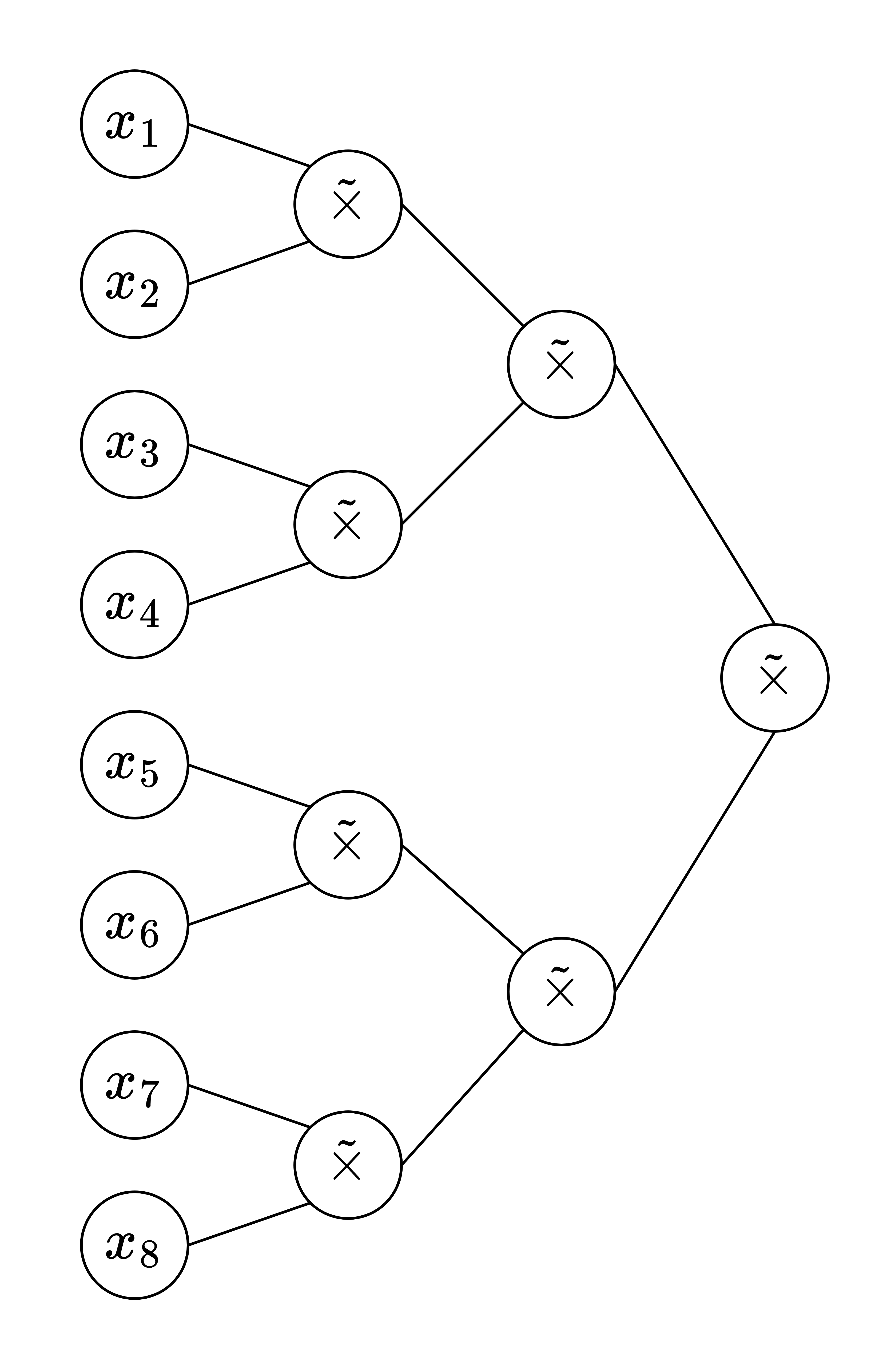
(a) $\tilde{\times}_{8}$

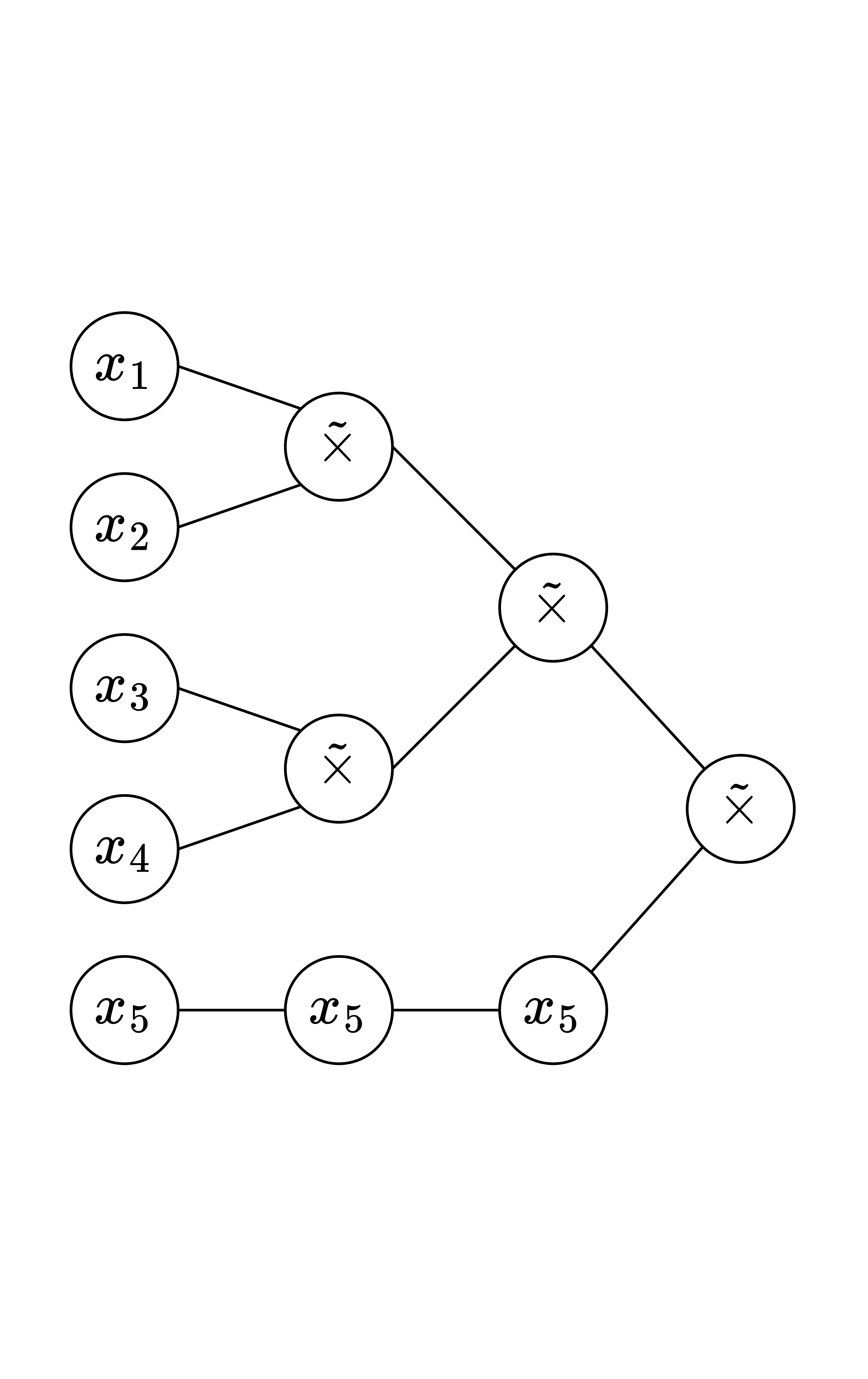
(b) $\tilde{\times}_{5}$

Figure 4: Network diagrams for ReLU networks approximating multiplication in Lemma 10.

Then $\tilde{\times}_{2^{i+1}}$ has depth $c\log\left(\frac{M^{2^{i+1}-2}}{\delta^{i}}\right)+c\log\left(\frac{M^{2^{i+1}}}{\delta}\right)=c\log\left(\frac{M^{2^{i+2}-2}}{\delta^{i+1}}\right)$, width $4\cdot 2^{i}+4\cdot 2^{i}=4\cdot 2^{i+1}$, and weights bounded by $M$. It remains to compute the following error bound:

$$|\tilde{\times}\left(\tilde{\times}_{2^{i}}(x_{1},\dots,x_{2^{i}}),\tilde{\times}_{2^{i}}(x_{2^{i}+1},\dots,x_{2^{i+1}})\right)-x_{1}\cdots x_{2^{i+1}}|$$

$$\leq|\tilde{\times}\left(\tilde{\times}_{2^{i}}(x_{1},\dots,x_{2^{i}}),\tilde{\times}_{2^{i}}(x_{2^{i}+1},\dots,x_{2^{i+1}})\right)-\tilde{\times}_{2^{i}}(x_{1},\dots,x_{2^{i}})\cdot\tilde{\times}_{2^{i}}(x_{2^{i}+1},\dots,x_{2^{i+1}})|$$

$$\quad+|\tilde{\times}_{2^{i}}(x_{1},\dots,x_{2^{i}})\cdot\tilde{\times}_{2^{i}}(x_{2^{i}+1},\dots,x_{2^{i+1}})-\tilde{\times}_{2^{i}}(x_{1},\dots,x_{2^{i}})\cdot x_{2^{i}+1}\cdots x_{2^{i+1}}|$$

$$\quad+|\tilde{\times}_{2^{i}}(x_{1},\dots,x_{2^{i}})\cdot x_{2^{i}+1}\cdots x_{2^{i+1}}-x_{1}\cdots x_{2^{i+1}}|$$

$$\leq\delta+|\tilde{\times}_{2^{i}}(x_{1},\dots,x_{2^{i}})|\cdot|\tilde{\times}_{2^{i}}(x_{2^{i}+1},\dots,x_{2^{i+1}})-x_{2^{i}+1}\cdots x_{2^{i+1}}|$$

$$\quad+|x_{2^{i}+1}\dots x_{2^{i+1}}|\cdot|\tilde{\times}_{2^{i}}(x_{1},\dots,x_{2^{i}})-x_{1}\cdots x_{2^{i}}|$$

$$\leq\delta+M^{2^{i}}(4^{i-1}M^{2^{i}-2}\delta)+M^{2^{i}}(4^{i-1}M^{2^{i}-2}\delta)\delta$$

$$=(1+24^{i-1}M^{2^{i+1}-2})\delta$$

$$<4^{i}M^{2^{i+1}-2}\delta.$$

From this, we have constructed a function $\tilde{\times}_{2^{k}}$ that approximates multiplication (of values $<M$) with error at most $4^{k-1}M^{2^{k}-2}\delta=\epsilon$ that has depth

$$c\log\left(\frac{M^{2^{k+1}-2}}{\delta^{k}}\right) =c\log\left(\frac{M^{2^{k}-2}M^{2^{k}}(4^{k-1})^{k}(M^{2^{k}-2})^{k}}{\epsilon^{k}}\right)$$

$$=c\log\left(M^{2^{k}-2}\right)+c\log\left(\frac{(4^{k-1})^{k}(M^{2^{k}})^{k}}{\epsilon^{k}}\right)$$

$$=c\log\left(M^{2^{k}-2}\right)+ck\log\left(\frac{4^{k-1}M^{2^{k}}}{\epsilon}\right)$$

$$<c(1+k)\log\left(\frac{4^{k-1}M^{2^{k}}}{\epsilon}\right)$$

$$<c_{1}k\log\left(\frac{4^{k-1}M^{2^{k}}}{\epsilon}\right),$$

For some absolute constant $c_{1}$. Now since $k=\log(d)$, we have that $M^{2^{k}}=M^{d}$ and $4^{k-1}<4^{k}=d^{2}$, so the ReLU network has depth at most $c\log(d)\log\left(\frac{d^{2}M^{d}}{\epsilon}\right)$ where $c$ is an absolute constant (the same constant as in Lemma 9). The width of $\tilde{\times}_{2^{k}}$ is $4\cdot 2^{k}=4d$, and the weights are bounded by $M$.

Figure 4(a) shows a neural network diagram for the ReLU network implementing $\tilde{\times}_{8}$, which has the structure of a full binary tree. In order to handle numbers that are not powers of two, we use an architecture similar to the diagram in Figure 4 (b) which depicts the ReLU network implementing $\tilde{\times}_{5}$.

Formally, suppose we have $2^{i-1}<d\leq 2^{i}$ for some $i\in\mathbb{N}$. Then consider the network $\tilde{\times}_{2^{i}}$ defined as before, but we remove the last $2^{i}-d$ input neurons, and replace them with $1$ everywhere they appear. Note that this can be achieved by adjusting the bias of each neuron appropriately. For example, any neuron can be turned into a constant 1 by making the weight vector $0$ and making the bias equal to $1$. This procedure will not affect the number of layers, it will not increase the width, and the parameters are bounded by $M+1<2M$. Noting that $2^{i}<2d$, we see that the ReLU network has width at most $4\cdot 2^{i}<4\cdot 2d=8d$. Finally, the depth is at most (for $c_{1}$ and $c_{2}$ absolute constants)

$$c\log(2^{i})\log\left(\frac{(2^{i})^{2}M^{d}}{\epsilon}\right) <c\log(2d)\log\left(\frac{(2d)^{2}M^{d}}{\epsilon}\right)$$

$$=c(\log(2)+\log(d))\left(\log(4)+\log\left(\frac{d^{2}M^{d}}{\epsilon}\right)\right)$$

$$<c\left(\log(8)+3\log(d)\log\left(\frac{d^{2}M^{d}}{\epsilon}\right)\right)$$

$$=c_{1}\log\left(\frac{d^{3}M^{d}}{\epsilon}\right)+c_{2}.$$

∎

Next we approximate the indicator functions of intervals (which we denote by $\mathds{1}_{(a,b)}$).

Lemma 11.

Fix $M>1$. Let $[a,b]\subseteq[-M,M]$ and $\epsilon<\frac{1}{2}(b-a)$. Then there is a ReLU network which implements a function $\tilde{\mathds{1}}_{(a,b)}^{\epsilon}$ such that

$$\left\|\tilde{\mathds{1}}_{(a,b)}^{\epsilon}-\mathds{1}_{(a,b)}\right\|_{L^{1}}=\epsilon.$$

This network has depth at most $c\log\left(\frac{1}{\epsilon}\right)$, width equal to 4, and weights bounded by $M$ (where $c$ is a constant depending only on $M$).

Proof.

We define the ReLU network function

$$\tilde{\mathds{1}}^{\epsilon}_{(a,b)}(x)=\frac{1}{\epsilon}(\sigma(x-(a-\epsilon))-\sigma(x-a)-\sigma(x-b)+\sigma(x-(b+\epsilon))),$$

where $\sigma$ is the ReLU activation function. Figure 5 is a plot of $\tilde{\mathds{1}}^{\epsilon}_{(a,b)}$. Then it is clear that

$$\left\|\tilde{\mathds{1}}^{\epsilon}_{(a,b)}-\mathds{1}_{(a,b)}\right\|_{L^{1}}=\epsilon.$$

Figure 5: Plot of $\tilde{\mathds{1}}^{\epsilon}_{(a,b)}$.

Note that we can express $\frac{1}{\epsilon}$ as

$$\frac{1}{\epsilon}=M^{\left\lceil\log_{M}\left(\frac{1}{\epsilon}\right)\right\rceil-1}\cdot\frac{\frac{1}{\epsilon}}{M^{\left\lceil\log_{M}\left(\frac{1}{\epsilon}\right)\right\rceil-1}}=\underbrace{M\times M\times\cdots\times M}_{\left\lceil\log_{M}\left(\frac{1}{\epsilon}\right)\right\rceil-1\text{ times}}\times R,$$

where $0<R\leq M$. This is a product of $\left\lceil\log_{M}\left(\frac{1}{\epsilon}\right)\right\rceil$ numbers that are all bounded by $M$. Then note that

$$\tilde{\mathds{1}}^{\epsilon}_{(a,b)}=M\times\dots\times M\times R(\sigma(x-(a-\epsilon))-\sigma(x-a)-\sigma(x-b)+\sigma(x-(b+\epsilon)))$$

can be implemented by ReLU network with $1+\left\lceil\log_{M}\left(\frac{1}{\epsilon}\right)\right\rceil$ layers. The first layer has $4$ neurons, and the second layer has one neuron, and they together compute $R(\sigma(x-(a-\epsilon))-\sigma(x-a)-\sigma(x-b)+\sigma(x-(b+\epsilon)))$. Then the next $\left\lceil\log_{M}\left(\frac{1}{\epsilon}\right)\right\rceil-1$ each multiply this value by $M$ (since all values at this point are positive, the ReLU activation does nothing at each layer). Thus the ReLU network has width $4$ (though only the first layer has more than one neuron) and weights bounded by $M$. ∎

We combine Lemma 10 and Lemma 11 to obtain an approximation to the indicator function of $d$-dimensional cube.

Lemma 12.

Fix $M>1$. Let $Q=\bigtimes_{k=1}^{d}(a_{k},b_{k})\subseteq[-M,M]^{d}$ be a bounded $d$-dimensional cube (i.e. $b_{1}-a_{1}=b_{k}-a_{k}$ for all $k\in[d]$), and suppose $\epsilon<\min\left(\frac{b_{1}-a_{1}}{2},1\right)$. Then there exists a function $\phi:[-M,M]^{d}\rightarrow\mathbb{R}$ implementable by a ReLU network such that

$$\int_{[-M,M]^{d}}|\mathds{1}_{Q}(x)-\phi(x)|\,dx<\epsilon.$$

The network has depth at most $c_{1}\log\left(\frac{d^{2}4^{d}}{\epsilon}\right)+c_{2}$, width at most $4d$, and weights bounded by $\max\{M,2\}$ (where $c_{1}$ and $c_{2}$ are constants only depending on $M$).

Proof.

Denote by $\tilde{\mathds{1}}^{\delta}_{(a_{i},b_{i})}$ the approximation to $\mathds{1}_{(a_{i},b_{i})}$ obtained from Lemma 11 with $\delta=\frac{\epsilon}{2}$. Let $\eta=\frac{\epsilon}{2^{d+1}M^{d}}$, and denote by $\tilde{\times}_{d}$ the approximation of the multiplication of $d$ factors obtained from Lemma 10 with parameters $M=1$ and error $\eta$ (which is denoted as $\epsilon$ in the lemma statement). Then we define $\phi$ by

$$\phi(x_{1},\dots,x_{d})=\tilde{\times}_{d}\left(\tilde{\mathds{1}}^{\delta}_{(a_{1},b_{1})}(x_{1}),\dots,\tilde{\mathds{1}}^{\delta}_{(a_{d},b_{d})}(x_{d})\right).$$

We compute

$$\int_{[-M,M]^{d}}\left|\mathds{1}_{\bigtimes_{i=1}^{d}[a_{i},b_{i})}(x)-\phi(x)\right|\,dx$$

$$=\int_{[-M,M]^{d}}\left|\prod_{i=1}^{d}\mathds{1}_{(a_{i},b_{i})}(x_{i})-\tilde{\times}_{d}\left(\tilde{\mathds{1}}^{\delta}_{(a_{1},b_{1})}(x_{1}),\dots,\tilde{\mathds{1}}^{\delta}_{(a_{d},b_{d})}(x_{d})\right)\right|\,dx$$

$$\leq\int_{[-M,M]^{d}}\left|\prod_{i=1}^{d}\mathds{1}_{(a_{i},b_{i})}(x_{i})-\prod_{i=1}^{d}\tilde{\mathds{1}}^{\delta}_{(a_{i},b_{i})}(x_{i})\right|\,dx$$

$$\quad\quad+\int_{[-M,M]^{d}}\left|\prod_{i=1}^{d}\tilde{\mathds{1}}^{\delta}_{(a_{i},b_{i})}(x_{i})-\tilde{\times}_{d}\left(\tilde{\mathds{1}}^{\delta}_{(a_{1},b_{1})}(x_{1}),\dots,\tilde{\mathds{1}}^{\delta}_{(a_{d},b_{d})}(x_{d})\right)\right|\,dx$$

$$<\int_{\bigtimes_{i=1}^{d}[a_{i}-\delta,b_{i}+\delta]\,\setminus\,\bigtimes_{i=1}^{d}[a_{i},b_{i})}\left|\prod_{i=1}^{d}\tilde{\mathds{1}}^{\delta}_{(a_{i},b_{i})}(x_{i})\right|+\int_{[-M,M]^{d}}\frac{\epsilon}{2^{d+1}M^{d}}\,dx$$

$$<\text{Vol}\left(\bigtimes_{i=1}^{d}(a_{i}-\delta,b_{i}+\delta)\,\setminus\,\bigtimes_{i=1}^{d}(a_{i},b_{i})\right)+\frac{\epsilon}{2}$$

where last inequality follows since $\left|\prod_{i=1}^{d}\tilde{\mathds{1}}^{\delta}_{(a_{i},b_{i})}(x_{i})\right|<1$. We now focus on bounding the measure of $R=\left(\bigtimes_{i=1}^{d}(a_{i}-\delta,b_{i}+\delta)\,\setminus\,\bigtimes_{i=1}^{d}(a_{i},b_{i})\right)$. First we express $R=\bigcup_{k=1}^{d}S_{k}^{+}\cup\bigcup_{k=1}^{d}S_{k}^{-}$ where

$$S_{k}^{-}=\left(\bigtimes_{i=1}^{k-1}(a_{i}-\delta,b_{i}+\delta)\right)\times(a_{k}-\delta,a_{k})\times\left(\bigtimes_{i=k+1}^{d}(a_{i}-\delta,b_{i}+\delta)\right),$$

$$S_{k}^{+}=\left(\bigtimes_{i=1}^{k-1}(a_{i}-\delta,b_{i}+\delta)\right)\times(b_{k},b_{k}+\delta)\times\left(\bigtimes_{i=k+1}^{d}(a_{i}-\delta,b_{i}+\delta)\right).$$

Thus we have that $\text{Vol}(R)\leq\sum_{k=1}^{d}\text{Vol}(S_{k}^{+})+\text{Vol}(S_{k}^{-})=2(2\delta+b_{i}-a_{i})^{d-1}\delta<2(2\delta+2M)^{d-1}\delta$. If we pick $\delta=\frac{\epsilon}{4(3M)^{d-1}}$, then we have

$$\|\mathds{1}_{Q}-\phi\|_{L^{1}} <\text{Vol}\left(\bigtimes_{i=1}^{d}(a_{i}-\delta,b_{i}+\delta)\,\setminus\,\bigtimes_{i=1}^{d}(a_{i},b_{i})\right)+\frac{\epsilon}{2}$$

$$\leq 2(2\delta+2M)^{d-1}\delta+\frac{\epsilon}{2}$$

$$=2(3M)^{d-1}\frac{\epsilon}{4(3M)^{d-1}}+\frac{\epsilon}{2}$$

$$=\frac{\epsilon}{2}+\frac{\epsilon}{2}=\epsilon.$$

Finally, we determine the size of $\phi$. Each $\tilde{\mathds{1}}^{\delta}_{(a_{i},b_{i})}$ can be implemented by a ReLU network with depth $c_{1}\log\left(\frac{1}{\delta}\right)=c_{1}\log\left(\frac{4\cdot 3^{d-1}M^{d-1}}{\epsilon}\right)\leq c_{2}\log\left(\frac{3^{d-1}M^{d-1}}{\epsilon}\right)$, width $4$, and weights bounded by $M$. $\tilde{\times}_{d}$ can be implemented by a ReLU network with depth at most

$$c_{3}\log\left(\frac{d^{3}2^{d}}{\eta}\right)+c_{4}=c_{3}\log\left(\frac{d^{3}2^{d}2^{d+1}M^{d}}{\epsilon}\right)+c_{4}=c_{3}\log\left(\frac{d^{3}2^{2d+1}M^{d}}{\epsilon}\right)+c_{4},$$

width at most 4d, and weights bounded by 2. Thus $\phi$ has width at most $4d$, weights bounded by $\max\{M,2\}$, and depth at most

$$c_{2}\log\left(\frac{3^{d-1}M^{d-1}}{\epsilon}\right)+c_{3}\log\left(\frac{d^{3}2^{2d+1}M^{d}}{\epsilon}\right)+c_{4}$$

$$<\max(c_{2},c_{3})\log\left(\frac{d^{3}3^{d-1}2^{2d+1}M^{2d-1}}{\epsilon^{2}}\right)+c_{4}$$

$$<\max(c_{2},c_{3})\log\left(\frac{d^{3}4^{d-1}4^{d+1}M^{2d}}{\epsilon^{2}}\right)+c_{4}$$

$$<\max(c_{2},c_{3})\log\left(\frac{(d^{2}4^{d}M^{d})^{2}}{\epsilon^{2}}\right)+c_{4}$$

$$=c_{5}\log\left(\frac{d^{2}4^{d}M^{d}}{\epsilon}\right)+c_{4}$$

$$=c_{5}\log\left(\frac{d^{2}4^{d}}{\epsilon}\right)+c_{5}d\log(M)+c_{4}.$$

$$<c_{6}\log\left(\frac{d^{2}4^{d}}{\epsilon}\right)+c_{4}.$$

∎

Now we use the construction of Lemma 12 to approximate the function from Lemma 8 as follows. Let $\{Q_{\vec{k}}\}_{\vec{k}\in[n]^{d}}$ be a decomposition of $[0,1]^{d}$ into almost non-overlapping cubes as in Lemma 8. The only overlap of these cubes is a set of measure $0$.

Lemma 13.

Let $0<\epsilon<\frac{1}{2n}$. Let $\{\beta_{\vec{k}}\}_{\vec{k}\in[n]^{d}}$ be constants within $[-M,M]$. Then the function $g$ defined by

$$g(x)=\sum_{k\in[n]^{d}}\beta_{\vec{k}}\mathds{1}_{Q_{\vec{k}}}(x)$$

can be approximated by a neural network $\tilde{g}$ with depth $c_{1}\log\left(\frac{d^{2}4^{d}n^{d}}{\epsilon}\right)+c_{2}$, width $4dn^{d}$, and weights bounded by $\max\{M,2\}$ (where $c_{1}$ and $c_{2}$ are constants only depending on $M$), such that

$$\int_{[-M,M]^{d}}|g(x)-\tilde{g}(x)|\,dx<\epsilon.$$

Proof.

For every $\vec{k}\in[n]^{d}$, let $\phi_{\vec{k}}$ be the function from Lemma 12 that approximates $\mathds{1}_{Q_{\vec{k}}}$ with error $\frac{\epsilon}{Mn^{d}}$. Then each $\phi_{\vec{k}}$ can be implemented by a ReLU network with

$$c_{1}\log\left(\frac{d^{2}4^{d}n^{d}M}{\epsilon}\right)+c_{2}=c_{1}\log\left(\frac{d^{2}4^{d}n^{d}}{\epsilon}\right)+c_{3}$$

layers, width at most $4d$, and weights bounded by $2$. This means we can implement the function $\tilde{g}(x)=\sum_{k\in[n]^{d}}\beta_{\vec{k}}\phi_{\vec{k}}$ by a ReLU network with one more layer, width at most $4dn^{d}$, and weights bounded by $\max\{M,2\}$. We compute

$$\int_{[-M,M]^{d}}|g(x)-\tilde{g}(x)|\,dx =\int_{[-M,M]^{d}}\left|\sum_{k\in[n]^{d}}\beta_{\vec{k}}\mathds{1}_{Q_{\vec{k}}}(x)-\sum_{k\in[n]^{d}}\beta_{\vec{k}}\phi_{\vec{k}}(x)\right|\,dx$$

$$\leq\sum_{k\in[n]^{d}}|\beta_{\vec{k}}|\int_{[-M,M]^{d}}\left|\mathds{1}_{Q_{\vec{k}}}(x)-\phi_{\vec{k}}(x)\right|\,dx$$

$$\leq\sum_{k\in[n]^{d}}|\beta_{\vec{k}}|\left(\frac{\epsilon}{Mn^{d}}\right)$$

$$\leq\sum_{k\in[n]^{d}}M\left(\frac{\epsilon}{Mn^{d}}\right)=\epsilon.$$

∎

A.3 Putting approximations together

We combine Lemma 8 with Lemma 13 to obtain our approximation result. The requirement of $d\geq 4$ in the following lemma is for technical reasons, and is not a requirement for Lemma 3 which is used in the main paper.

Lemma 14.

Suppose $f\in C^{\alpha}([0,1]^{d})$, $\alpha\in(0,1)$, with $\|f\|_{L^{\infty}}<M$ and $M\geq 2$. Assume further that $d\geq 4$. Let $\epsilon>0$. Then there exists a function $\Phi$ implementable by a ReLU network such that

$$\|f-\Phi\|_{L^{1}}<\epsilon.$$

The ReLU network has depth at most $c_{1}d\log\left(\frac{8d\|f\|_{C^{\alpha}}^{1/\alpha}}{\epsilon^{2/\alpha}}\right)+c_{2}$, width at most $\frac{(4d)^{d/2}\|f\|_{C^{\alpha}}^{d/\alpha}}{\epsilon^{d/\alpha}}$, and weights bounded by $M$ (where $c_{1}$ and $c_{2}$ are constants only depending on $M$).

Proof.

Let $n=\left\lceil\left(\frac{\|f\|_{C^{\alpha}}}{\epsilon}\right)^{1/\alpha}\sqrt{d}\right\rceil$. Let $f^{n}$ be the piecewise constant function from Lemma 8. Notice that $f^{n}$ follows the same form as the function $g$ in Lemma 13. By Lemma 13, there is a ReLU network function $\Phi$ that approximates $f^{n}$ such that

$$\int_{[-M,M]^{d}}|f^{n}(x)-\Phi(x)|\,dx<\frac{\epsilon}{2}.$$

Then we compute

$$\|f-\Phi\|_{L^{1}}\leq\|f-f^{n}\|_{L^{1}}+\|f^{n}-\Phi\|_{L^{1}}<\frac{\|f\|_{C^{\alpha}}d^{\alpha/2}}{n^{\alpha}}+\frac{\epsilon}{2}<\frac{\epsilon}{2}+\frac{\epsilon}{2}=\epsilon.$$

Note that $\Phi$ has width $4dn^{d}<4d\left(2\left(\frac{\|f\|_{C^{\alpha}}}{\epsilon}\right)^{1/\alpha}\sqrt{d}\right)^{d}=c_{0}\frac{(4d)^{d/2}\|f\|_{C^{\alpha}}^{d/\alpha}}{\epsilon^{d/\alpha}}$, and the weights of $\Phi$ are bounded by $M$. The depth of $\Phi$ is bounded by

$$c_{1}\log\left(\frac{d^{2}4^{d}n^{d}}{\epsilon}\right)+c_{2} <c_{1}\log\left(\frac{d^{2}4^{d}\|f\|_{C^{\alpha}}^{\frac{d}{\alpha}}2^{d}d^{\frac{d}{2}}}{\epsilon\epsilon^{\frac{d}{\alpha}}}\right)+c_{2}$$

$$<c_{1}\log\left(\frac{d^{d}8^{d}\|f\|_{C^{\alpha}}^{\frac{d}{\alpha}}}{\epsilon^{\frac{2d}{\alpha}}}\right)+c_{2}$$

$$=c_{1}d\log\left(\frac{8d\|f\|_{C^{\alpha}}^{1/\alpha}}{\epsilon^{2/\alpha}}\right)+c_{2}$$

where we use the fact that $d\geq 4$ to bound $2+\frac{d}{2}\leq d$.

∎

In the main paper, we use Lemma 3, which is proved below.

Proof of Lemma 3.

By allowing the constants to depend on all values except $\epsilon$, the depth of the ReLU network $\Phi$ from Lemma 14 can be expressed as

$$c_{1}d\log\left(\frac{8d\|f\|^{1/\alpha}_{C_{\alpha}}}{\epsilon^{2/\alpha}}\right)+c_{2}=c_{3}\left(\log\left(\frac{1}{\epsilon^{2/\alpha}}\right)+\log\left(8d\|f\|^{1/\alpha}_{C_{\alpha}}\right)\right)+c_{2}=\frac{2}{\alpha}c_{3}\log\left(\frac{1}{\epsilon}\right)+c_{4}<c_{5}\log\left(\frac{1}{\epsilon}\right),$$

and the width can be expressed as

$$\frac{(4d)^{d/2}\|f\|_{C^{\alpha}}^{d/\alpha}}{\epsilon^{d/\alpha}}=\frac{c_{6}}{\epsilon^{d/\alpha}}.$$

∎

Appendix B An Alternative Approach: Voronoi Decompositions

In this section we sketch an alternative approach to our approximation theory which decomposes the manifold into Voronoi cells and transports onto each disjoint cell directly. This theory is not complete as we have not ruled out the existence of particularly pathological cells which lack an open kernel in tangent space. However we believe such an approach is workable, though very technical, and has benefits associated with a disjoint Voronoi decomposition of the manifold. Therefore we present a sketch of our ideas.

Recall our goal in approximation theory is to construct a transport map $g^{*}:(0,1)^{d+1}\to\mathcal{M}$ that can be approximated by neural networks. First, we partition the manifold into geodesic Voronoi cells and map local distributions over the cells onto tangent planes. Then we transform the distribution on tangent planes to a distribution on a ball from which we can apply optimal transport theory to produce a map between the source distribution on $(0,1)^{d}$ to a ball. Finally we glue together these local maps with indicators and a uniform random sample from $(0,1)$. We proceed with the first step of partitioning the manifold.

Step 1: Voronoi decomposition. Given $\mathcal{M}$ under Assumption 1, we decompose $\mathcal{M}$ into a partition of finite geodesic Voronoi cells. This is done by first covering $\mathcal{M}$ with Euclidean balls around each point with uniform radius less than the global injectivity radius. Via compactness we can extract a finite subcover $\{U_{j}\}_{j=1}^{J}$ with centers $\{c_{j}\}_{j=1}^{J}$. We form a Voronoi partition of $\mathcal{M}$ denoted $\{V_{j}\}$ by taking the $c_{j}$ as centers, i.e.

$$V_{j}=\{x\in\mathcal{M}:d_{\mathcal{M}}(x,c_{j})=\textstyle\min_{i\in[J]}d_{\mathcal{M}}(x,c_{i})\}.$$

A Voronoi decomposition is illustrated in Figure 7. Note the boundary/overlap of the cells has measure $0$ with respect to $Q$. We check this later in the appendix. Now, given a distribution $Q$ on $\mathcal{M}$ with density $q$, we can define local distributions $Q_{j}$ as the conditional distribution of $Q$ on $V_{j}$.

For any measurable set $A$, we have

$$Q(A)=\sum_{j=1}^{J}Q(A\cap V_{j})=\sum_{j=1}^{j}Q(V_{j})Q(A|V_{j})=\sum_{j=1}^{j}Q(V_{j})Q_{j}(A).$$

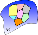
Figure 6: A Voronoi decomposition of $\mathcal{M}$.

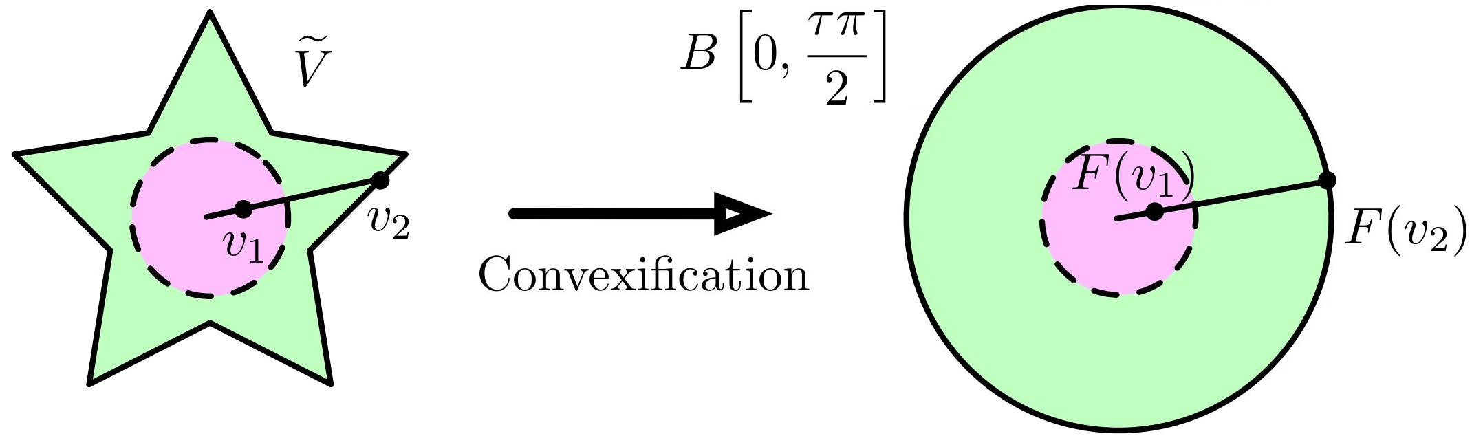
Figure 7: Expansion of star-shaped set into ball via $F$.

Step 2: Defining local lower-dimensional distributions. Next we transform local distribution $Q_{j}$ on $V_{j}$ into a distribution $\tilde{Q}_{j}$ on $\tilde{V}_{j}=\exp_{c_{j}}^{-1}(V_{j})$ which is inverse of image of the $j$th Voronoi cell under the exponential map. In particular $Q_{j}$ is the pushforward of $\tilde{Q}_{j}$ by the exponential map. The density of $\tilde{Q}_{j}$ given by

$$\tilde{q}_{j}(v)=q_{j}(\exp_{c_{j}}(v))\left|\det J_{\exp_{c_{j}}}(v)\right|$$

via an application of formula (5). For simplicity, we use $\det J_{\exp_{c_{j}}}(v)$ to denote the Jacobian $\sqrt{\det g_{ij}^{x}(v)}$. $\tilde{Q}_{j}$ has two important properties. First, $\tilde{q}_{j}$ continues to be upper and lower-bounded and so we can still hope to apply optimal transport theory. Second, $\tilde{V}_{j}\subseteq T_{c_{j}}\mathcal{M}$ is a $d$-dimensional set on which $(\exp_{c_{j}})_{\sharp}\tilde{Q}_{j}=Q_{j}$. Ideally, to apply optimal transport theory, the target domain $\tilde{V}_{j}$ needs to be convex. However, $\tilde{V}_{j}$ is not convex here, but it is star-shaped. Recall a set $S$ is star-shaped if $\exists$ $x\in S$ such that for all $y\in S$, the set $[x:y]=\{\lambda x+(1-\lambda)y:\lambda\in[0,1]\}\subseteq S$. For an excellent reference on star-shaped sets see Hansen et al. [2020]. This property is crucial and allows us to transform our target domain $\tilde{V}_{j}$ to a ball via a bi-Lipschitz transformation.

Step 3: Convexifying the Target Domain $\tilde{V}_{j}$. As we claim above, the target domain $\tilde{V}_{j}$ is star-shaped and centered at 0. $\tilde{V}_{j}$ is also bounded and closed and hence compact. Further we know for some $\eta>0$, $B(0,\eta)\subseteq\tilde{V}_{j}$. Then we can apply the following lemma to produce a bi-Lipschitz transformation $F:\tilde{V}_{j}\to B\left(0,\frac{\tau\pi}{2}\right)$, where $\tau$ is the reach of $\mathcal{M}$.

Lemma 15.

Let $S$ be a compact star-shaped set centered at $0$. Further suppose $\exists\eta>0$ such that $B(0,\eta)\subseteq S$. Let $L>0$ be such that $S\subseteq B[0,L]$. Then there exists $F:S\to B[0,L]$ such that $F$ is bi-Lipschitz with constant $C$ dependent on $L,\eta$.

Lemma 15 is proved in Appendix B.1. The main idea is that the bi-Lipschitz map is constructed explicitly by expanding along rays (see Figure 7). Theorem 1 from Toranzos [1967] tells us the radial function on $S$ which computes the radius of $\tilde{V}_{j}$ in a direction $u\in\mathbb{S}^{d-1}$ is Lipschitz when the star-shaped set is compact and contains a nontrivial interior kernel. We recall the kernel of a star-shaped is the set of points which have visibility to all points in the set. We believe appropriately chosen manifold Voronoi cells will have non-empty interior kernel. However this remains a technical difficulty.

From this we can construct bi-Lipschitz $F_{j}$ by fixing points in a ball of radius ${\eta}/{2}$ and expanding points at a rate dependent on its distance from $B(0,\eta/2)$ and $R(x)$. Note that we apply Lemma 15 to obtain a map from the closure of $\tilde{V}_{j}$ to $B\left[0,\frac{\tau\pi}{2}\right]$, which we can then restrict to $\tilde{V}_{j}$ to obtain a bi-Lipschitz map from $\tilde{V}_{j}$ to $B(0,L)$. We can define a new distribution $\tilde{\rho}_{j}$ on $B\left(0,\frac{\tau\pi}{2}\right)$ with density

$$\tilde{p}_{j}(x)=\tilde{q}(F_{j}^{-1}(x))\left|\det J_{{F_{j}^{-1}}}(x)\right|.$$

It is important $F_{j}$ is bi-Lipschitz with constant $C$ as then $\frac{1}{C^{d}}\leq|\det J_{F_{j}}(x)|\leq C^{d}$ and we know $\tilde{p}_{j}$ is upper and lower-bounded. Further we can write $(F^{-1}_{j})_{\sharp}\tilde{\rho}_{j}=\tilde{Q}_{j}$ by $g_{j}^{*}$.

Step 4: Constructing the local transport. Now we have a distribution $\tilde{\rho}_{j}$ with density $\tilde{p}_{j}$ defined on convex ball $B\left(0,\frac{\tau\pi}{2}\right)$. Further $\tilde{p}_{j}$ is upper and lower bounded. Set $\rho_{d}$ to be uniform on $(0,1)^{d}$. Hence we may apply Proposition 1 to produce a transport map $T_{j}:(0,1)^{d}\to B\left(0,\frac{\tau\pi}{2}\right)$ such that $(T_{j})_{\sharp}\rho_{d}=\tilde{\rho}$. Further $T_{j}$ is Hölder with Hölder exponent $\alpha_{j}$ for some $\alpha_{j}\in(0,1)$. Writing $g_{j}^{*}:(0,1)^{d}\to V_{j}$ via

$$g_{j}^{*}(x)=\exp_{c_{j}}\circ F_{j}^{-1}\circ T_{j}(x)$$ (16)

gives rise to $(g_{j}^{*})_{\sharp}\rho_{d}=Q_{j}.$ This transport map $g_{j}^{*}$ is illustrated in Figure 8. Further $g_{j}^{*}$ is the composition of two Lipschitz functions with an $\alpha_{j}$-Hölder continuous function and is therefore $\alpha_{j}$-Hölder continuous. Thus we can push a uniform distribution on $(0,1)^{d}$ onto a local patch $V_{j}$, as shown in Figure 8.

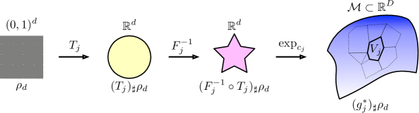
Figure 8: Local transport $g_{j}^{*}$ in (16) mapping $\rho_{d}$ on $(0,1)^{d}$ to a local distribution $\mathcal{M}$ supported on $V_{j}$.

Step 5: Constructing the global transport. Via step 4 we have local transports $g_{j}^{*}$ pushing forward $\rho_{d}$ uniform on $(0,1)^{d}$ to local distribution $Q_{j}$. By setting $\pi_{j}=Q(\bigcup_{i=1}^{j}V_{i})$. Now we define $g^{*}:(0,1)^{d+1}\to\mathcal{M}$ via (6)

$$g^{*}(x)=\sum_{j=1}^{J}\mathds{1}_{[\pi_{j-1},\pi_{j})}(x_{1})g^{*}_{j}(x_{2:d+1})$$

where $x_{1}$ is the first component of $x$ and $x_{2:d+1}$ are the remaining components.

Set $X\sim\rho$. Then $X_{1}$ randomly selects the patch $V_{j}$ with probability equal to $Q(V_{j})$, and $g_{j}^{*}$ pushes $X_{2:d+1}$ forward to $V_{j}$ such that $g_{j}^{*}(X_{2:d+1})$ is distributed according to $Q_{j}$. Finally note that the overlap of of the Voronoi cells $V_{i}$ and $V_{j}$ while $i\neq j$ has measure $0$. Hence $g^{*}(X)$ is distributed on $\mathcal{M}$ according to $Q$. This constructs the oracle $g^{*}$. Furthermore, we note that each of the $g_{j}^{*}$ is $\alpha_{j}$-Hölder continuous, so by setting $\alpha=\min_{j}\alpha_{j}$ we obtain that all of the $g_{j}^{*}$ are $\alpha$-Hölder continuous, which complete the proof of Lemma 1.

B.1 Proof of Lemma 15

Proof.

We will construct a bi-Lipschitz map from a compact star-shaped set centered at $0$ to a closed ball. Define the radial map $r:\mathbb{S}^{n-1}\to\mathbb{R}$ via $r(u)=\sup\{\lambda:\lambda u\in S\}$. Along a direction this gives us the radius of the set. Then via Toranzos [1967] this map is Lipschitz with optimal constant $C_{1}=L\sqrt{\left(\frac{L}{\delta}\right)^{2}-1}$. Write $R(x)=r\left(\frac{x}{\|x\|}\right)$. We use this to define a function $A(x)$ on $S\backslash B(0,\delta/2)$ such that $A(x)=x$ if $\|x\|=\frac{\delta}{2}$ and $A(x)=L\frac{x}{\|x\|}$ if $\|x\|=R(x)$. Set $A:S\backslash B\left(0,\frac{\delta}{2}\right)\to B(0,L)$ via

$$A(x)=\left(\frac{\delta}{2}+\frac{L-\frac{\delta}{2}}{R(x)-\frac{\delta}{2}}\left(\|x\|-\frac{\delta}{2}\right)\right)\frac{x}{\|x\|}.$$

We observe some properties of $A$. First, $A$ expands along rays meaning we can write $A(x)=\lambda_{x}x$ for some $\lambda$ dependent on $x$. Next, $A$ satisfies $A(x)=x$ when $\|x\|=\frac{\delta}{2}$ and $A(x)=L\frac{x}{\|x\|}$ when $\|x\|=R(x)$. Also, on a direction $u\in\mathbb{S}^{n-1}$ we have $A$ is strictly increasing in norm and hence injective on each ray. Thus $A$ is injective in total. Further, $A$ is surjective via an application of intermediate value theorem and we can write the inverse explicitly as

$$A^{-1}(x)=\left(\frac{\delta}{2}+\frac{R(x)-\frac{\delta}{2}}{L-\frac{\delta}{2}}\left(\|x\|-\frac{\delta}{2}\right)\right)\frac{x}{\|x\|}.$$

We verify this is the inverse by choosing $y=A(x)$ for some $x$ in the domain. Then

$$\|y\|=\frac{\delta}{2}+\frac{R(x)-\frac{\delta}{2}}{L-\frac{\delta}{2}}\left(\|x\|-\frac{\delta}{2}\right).$$

Write $z=A^{-1}(y)$ and compute the norm as

$$\|z\| =\left(\frac{\delta}{2}+\frac{R(x)-\frac{\delta}{2}}{L-\frac{\delta}{2}}\left(\|y\|-\frac{\delta}{2}\right)\right)$$

$$=\left(\frac{\delta}{2}+\frac{R(x)-\frac{\delta}{2}}{L-\frac{\delta}{2}}\left(\left(\frac{\delta}{2}+\frac{L-\frac{\delta}{2}}{R(x)-\frac{\delta}{2}}\left(\|x\|-\frac{\delta}{2}\right)\right)-\frac{\delta}{2}\right)\right)$$

$$=\left(\frac{\delta}{2}+\frac{R(x)-\frac{\delta}{2}}{L-\frac{\delta}{2}}\left(\frac{L-\frac{\delta}{2}}{R(x)-\frac{\delta}{2}}\left(\|x\|-\frac{\delta}{2}\right)\right)\right)$$

$$=\left(\frac{\delta}{2}+\frac{R(x)-\frac{\delta}{2}}{L-\frac{\delta}{2}}\left(\frac{L-\frac{\delta}{2}}{R(x)-\frac{\delta}{2}}\left(\|x\|-\frac{\delta}{2}\right)\right)\right)$$

$$=\frac{\delta}{2}+\|x\|-\frac{\delta}{2}=\|x\|.$$

Since $A$ expands along rays we have $z=x$ as desired.

We can then define the functions $F_{1}:S\backslash B\left(0,\frac{\delta}{2}\right)\to B[0,L]$ and $F_{2}:B\left[0,\frac{\delta}{2}\right]\to B[0,L]$ via $F_{1}(x)=A(x)$ and $F_{2}(x)=x$. Note immediately $F_{2}$ is bi-Lipschitz with constant $1$.

Further we argue $A(x)$ is bi-Lipschitz. As a necessary warm-up we show $R(x)=r\left(\frac{x}{\|x\|}\right)$ is Lipschitz. We know $x\rightarrow\|x\|$ is Lipschitz with constant $1$, and $\|x\|\rightarrow\frac{1}{\|x\|}$ on $\left[\frac{\delta}{2},\infty\right)$ is Lipschitz away from $0$ with constant $\frac{4}{\delta^{2}}$, and $r(\cdot)$ is Lipschitz with constant $C_{1}$ given above. Now for $x,y\in S$ we have

$$|R(x)-R(y)| =\left|r\left(\frac{x}{\|x\|}\right)-r\left(\frac{y}{\|y\|}\right)\right|$$

$$\leq C_{1}\left\|\frac{x}{\|x\|}-\frac{y}{\|y\|}\right\|$$

$$\leq C_{1}\left(\left\|\frac{x}{\|x\|}-\frac{x}{\|y\|}\right\|+\left\|\frac{x}{\|y\|}-\frac{y}{\|y\|}\right\|\right)$$

$$\leq C_{1}\left(L\left|\frac{1}{\|x\|}-\frac{1}{\|y\|}\right|+\frac{2}{\delta}\|x-y\|\right)$$

$$\leq C_{1}\left(L\frac{4}{\delta^{2}}\|x-y\|+\frac{2}{\delta}\|x-y\|\right)$$

$$\leq C_{1}\left(\frac{4L}{\delta^{2}}+\frac{2}{\delta}\right)\|x-y\|$$

as desired. Notice it is important that the set $S$ is bounded and the operator $R$ is defined at a radius $\frac{\delta}{2}$ away from $0$. Using this we can show $A$ is Lipschitz. Clearly $\|x\|-\frac{\delta}{2}$ is Lipschitz and bounded since $S$ is bounded. $\frac{1}{R(x)-\frac{\delta}{2}}$ will be Lipschitz as $R(x)-\frac{\delta}{2}$ is Lipschitz and we have $R(x)\geq\delta$ so the denominator is lower bounded. Thus $\frac{L-\frac{\delta}{2}}{R(x)-\frac{\delta}{2}}(\|x\|-\frac{\delta}{2})$ is Lipschitz as the product of bounded Lipschitz functions. It follows $A$ is Lipschitz, as the product of bounded Lipschitz functions, with some constant $C_{2}$. A nearly identical argument shows $A^{-1}$ is Lipschitz. Hence $F_{1}$ is bi-Lipschitz.

Define a function $F$ on $S$ as $F_{1}$ on $S\backslash B(0,\delta/2)$ and $F_{2}$ on $B(0,\delta/2)$. This will be Lipschitz as $F$ is Lipschitz on each of the two domains and for $x\in S\backslash B(0,\delta/2),y\in B(0,\delta/2)$ we have

$$|F(x)-F(y)| \leq|F(x)-F(z)|+|F(z)-F(y)|\leq C_{2}\|x-z\|+\|z-y\|$$

$$\leq C_{2}\|x-y\|+\|x-y\|=(C_{2}+1)\|x-y\|$$

where we pick $z\in[x:y]\cap B(0,\delta/2)$ and recall $[x:y]$ is the line between $x$ and $y$. Hence $|x-z|,|y-z|\leq|x-y|$. This shows $F$ Lipschitz. It is also clearly bijective as each of its components are bijective and we can write $F^{-1}$ explicitly. A similar argument shows $F^{-1}$ is Lipschitz. Thus $F$ is bi-Lipschitz. ∎

B.2 Voronoi cells have measure 0 overlap

Proof.

We have that $Q(V_{i}\cap V_{j})=0$. To see this, it suffices to show the set of points $I_{ij}=\{x\in U_{i}\cap U_{j}:d_{\mathcal{M}}(x,c_{i})=d_{\mathcal{M}}(x,c_{j})\}$ is a codim 1 submanifold of $M$, which means it has Hausdorff measure 0. Note that $I_{ij}=f_{ij}^{-1}(0)$ where $f_{ij}:U_{i}\cap U_{j}\rightarrow\mathbb{R}:x\mapsto d_{\mathcal{M}}^{2}(c_{i},x)-d_{\mathcal{M}}^{2}(c_{j},x)$, so it suffices to show that $0$ is a regular value of $f_{ij}$ which is smooth in $U_{i}\cap U_{j}$. Note that $df_{x}=-2(\exp_{x}^{-1}(c_{i})-\exp_{x}^{-1}(c_{j}))$. For all $x\in f^{-1}_{ij}(0)$, we need to show that $df_{x}$ has full rank. Since the co-domain of $df_{x}$ is one dimensional, this is equivalent to showing that $df_{x}\neq 0$. Suppose for the sake of contradiction that $df_{x}=0$. Then this implies $\exp_{x}^{-1}(c_{i})=\exp_{x}^{-1}(c_{j})$. Since $\exp_{x}$ is a diffeomorphism in a neighborhood that includes $c_{i}$ and $c_{j}$, this implies that $c_{i}=c_{j}$. But this is not true for $i\neq j$. Thus $df_{x}$ is full rank for all $x\in U_{i}\cap U_{j}$ such that $f(x)=0$, so $0$ is a regular value of $f$. ∎

References

- Aamari and Levrard [2019] Eddie Aamari and Clément Levrard. Nonasymptotic rates for manifold, tangent space and curvature estimation. The Annals of Statistics, 2019.
- Aamari et al. [2019] Eddie Aamari, Jisu Kim, Frédéric Chazal, Bertrand Michel, Alessandro Rinaldo, Larry Wasserman, et al. Estimating the reach of a manifold. Electronic Journal of Statistics, 13(1):1359–1399, 2019.
- Arjovsky et al. [2017] Martin Arjovsky, Soumith Chintala, and Léon Bottou. Wasserstein generative adversarial networks. In International conference on machine learning, pages 214–223. PMLR, 2017.
- Arora et al. [2017] Sanjeev Arora, Rong Ge, Yingyu Liang, Tengyu Ma, and Yi Zhang. Generalization and equilibrium in generative adversarial nets (gans). arXiv preprint arXiv:1703.00573, 2017.
- Bai et al. [2018] Yu Bai, Tengyu Ma, and Andrej Risteski. Approximability of discriminators implies diversity in gans. arXiv preprint arXiv:1806.10586, 2018.
- Block et al. [2021] Adam Block, Zeyu Jia, Yury Polyanskiy, and Alexander Rakhlin. Intrinsic dimension estimation. arXiv preprint arXiv:2106.04018, 2021.
- Brock et al. [2018] Andrew Brock, Jeff Donahue, and Karen Simonyan. Large scale gan training for high fidelity natural image synthesis. arXiv preprint arXiv:1809.11096, 2018.
- Caffarelli [1992] Luis A Caffarelli. The regularity of mappings with a convex potential. Journal of the American Mathematical Society, 5(1):99–104, 1992.
- Chae et al. [2021] Minwoo Chae, Dongha Kim, Yongdai Kim, and Lizhen Lin. A likelihood approach to nonparametric estimation of a singular distribution using deep generative models. arXiv preprint arXiv:2105.04046, 2021.
- Chen et al. [2019] Minshuo Chen, Haoming Jiang, Wenjing Liao, and Tuo Zhao. Nonparametric regression on low-dimensional manifolds using deep relu networks. arXiv: Learning, 2019.
- Chen et al. [2020] Minshuo Chen, Wenjing Liao, Hongyuan Zha, and Tuo Zhao. Statistical guarantees of generative adversarial networks for distribution estimation. CoRR, abs/2002.03938, 2020. URL https://arxiv.org/abs/2002.03938.
- Coifman et al. [2005] Ronald R Coifman, Stephane Lafon, Ann B Lee, Mauro Maggioni, Boaz Nadler, Frederick Warner, and Steven W Zucker. Geometric diffusions as a tool for harmonic analysis and structure definition of data: Diffusion maps. Proceedings of the national academy of sciences, 102(21):7426–7431, 2005.
- Evans and Gariepy [1992] L. C. Evans and R. F. Gariepy. Measure theory and fine properties of functions. 1992.
- Federer [1959] Herbert Federer. Curvature measures. Transactions of the AMS, pages 418–494, 1959.
- Flaherty and do Carmo [2013] F. Flaherty and M.P. do Carmo. Riemannian Geometry. Mathematics: Theory & Applications. Birkhäuser Boston, 2013. ISBN 9780817634902. URL https://books.google.com/books?id=ct91XCWkWEUC.
- Frogner et al. [2015] Charlie Frogner, Chiyuan Zhang, Hossein Mobahi, Mauricio Araya, and Tomaso A Poggio. Learning with a wasserstein loss. Advances in neural information processing systems, 28, 2015.
- Genevay et al. [2018] Aude Genevay, Gabriel Peyré, and Marco Cuturi. Learning generative models with sinkhorn divergences. In International Conference on Artificial Intelligence and Statistics, pages 1608–1617. PMLR, 2018.
- Goodfellow et al. [2014] Ian Goodfellow, Jean Pouget-Abadie, Mehdi Mirza, Bing Xu, David Warde-Farley, Sherjil Ozair, Aaron Courville, and Yoshua Bengio. Generative adversarial nets. pages 2672–2680, 2014.
- Hansen et al. [2020] G. Hansen, Irmina Herburt, H. Martini, and M. Moszyńska. Starshaped sets. Aequationes mathematicae, 94, 12 2020. doi: 10.1007/s00010-020-00720-7.
- Huang et al. [2022] Jian Huang, Yuling Jiao, Zhen Li, Shiao Liu, Yang Wang, and Yunfei Yang. An error analysis of generative adversarial networks for learning distributions. Journal of Machine Learning Research, 23(116):1–43, 2022.
- Jiang et al. [2018] Haoming Jiang, Zhehui Chen, Minshuo Chen, Feng Liu, Dingding Wang, and Tuo Zhao. On computation and generalization of gans with spectrum control. arXiv preprint arXiv:1812.10912, 2018.
- Kingma and Welling [2013] DP Kingma and M Welling. Auto-encoding variational bayes. iclr 2014 2014. arXiv preprint arXiv:1312.6114, 2013.
- Ledig et al. [2017] Christian Ledig, Lucas Theis, Ferenc Huszár, Jose Caballero, Andrew Cunningham, Alejandro Acosta, Andrew Aitken, Alykhan Tejani, Johannes Totz, Zehan Wang, et al. Photo-realistic single image super-resolution using a generative adversarial network. In Proceedings of the IEEE conference on computer vision and pattern recognition, pages 4681–4690, 2017.
- Liang [2017] Tengyuan Liang. How well can generative adversarial networks learn densities: A nonparametric view. arXiv preprint arXiv:1712.08244, 2017.
- Liang [2018] Tengyuan Liang. On how well generative adversarial networks learn densities: Nonparametric and parametric results. arXiv preprint arXiv:1811.03179, 2018.
- Lu and Lu [2020] Yulong Lu and Jianfeng Lu. A universal approximation theorem of deep neural networks for expressing probability distributions. Advances in neural information processing systems, 33:3094–3105, 2020.
- Luise et al. [2020] Giulia Luise, Massimiliano Pontil, and Carlo Ciliberto. Generalization properties of optimal transport gans with latent distribution learning. arXiv preprint arXiv:2007.14641, 2020.
- Mohamed and Wierstra [2014] Shakir Mohamed and Daan Wierstra. Stochastic backpropagation and approximate inference in deep generative models. 2014.
- Müller [1997] Alfred Müller. Integral probability metrics and their generating classes of functions. Advances in Applied Probability, 29(2):429–443, 1997. ISSN 00018678. URL http://www.jstor.org/stable/1428011.
- Ohn and Kim [2019] Ilsang Ohn and Yongdai Kim. Smooth function approximation by deep neural networks with general activation functions. Entropy, 21(7):627, 2019.
- Peyré [2009] Gabriel Peyré. Manifold models for signals and images. Computer vision and image understanding, 113(2):249–260, 2009.
- Radford et al. [2015] Alec Radford, Luke Metz, and Soumith Chintala. Unsupervised representation learning with deep convolutional generative adversarial networks. arXiv preprint arXiv:1511.06434, 2015.
- Reed et al. [2016] Scott Reed, Zeynep Akata, Xinchen Yan, Lajanugen Logeswaran, Bernt Schiele, and Honglak Lee. Generative adversarial text to image synthesis. arXiv preprint arXiv:1605.05396, 2016.
- Roweis and Saul [2000] Sam T Roweis and Lawrence K Saul. Nonlinear dimensionality reduction by locally linear embedding. science, 290(5500):2323–2326, 2000.
- Salimans et al. [2016] Tim Salimans, Ian Goodfellow, Wojciech Zaremba, Vicki Cheung, Alec Radford, and Xi Chen. Improved techniques for training gans. In Advances in neural information processing systems, pages 2234–2242, 2016.
- Schawinski et al. [2017] Kevin Schawinski, Ce Zhang, Hantian Zhang, Lucas Fowler, and Gokula Krishnan Santhanam. Generative adversarial networks recover features in astrophysical images of galaxies beyond the deconvolution limit. Monthly Notices of the Royal Astronomical Society: Letters, 467(1):L110–L114, 2017.
- Schreuder et al. [2021] Nicolas Schreuder, Victor-Emmanuel Brunel, and Arnak Dalalyan. Statistical guarantees for generative models without domination. In Algorithmic Learning Theory, pages 1051–1071. PMLR, 2021.
- Shen et al. [2022] Zuowei Shen, Haizhao Yang, and Shijun Zhang. Optimal approximation rate of relu networks in terms of width and depth. Journal de Mathématiques Pures et Appliquées, 157:101–135, 2022.
- Tenenbaum et al. [2000] Joshua B Tenenbaum, Vin De Silva, and John C Langford. A global geometric framework for nonlinear dimensionality reduction. science, 290(5500):2319–2323, 2000.
- Toranzos [1967] F. A. Toranzos. Radial functions of convex and star-shaped bodies. The American Mathematical Monthly, 74(3):278–280, 1967. ISSN 00029890, 19300972. URL http://www.jstor.org/stable/2316022.
- Uppal et al. [2019] Ananya Uppal, Shashank Singh, and Barnaás Póczos. Nonparametric density estimation & convergence of gans under besov ipm losses. arXiv preprint arXiv:1902.03511, 2019.
- Villani [2008] Cédric Villani. Optimal transport: old and new, volume 338. Springer Science & Business Media, 2008.
- Volz et al. [2018] Vanessa Volz, Jacob Schrum, Jialin Liu, Simon M Lucas, Adam Smith, and Sebastian Risi. Evolving mario levels in the latent space of a deep convolutional generative adversarial network. In Proceedings of the Genetic and Evolutionary Computation Conference, pages 221–228, 2018.
- Weed and Bach [2019] Jonathan Weed and Francis R. Bach. Sharp asymptotic and finite-sample rates of convergence of empirical measures in wasserstein distance. Bernoulli, 2019.
- Yang et al. [2022] Yunfei Yang, Zhen Li, and Yang Wang. On the capacity of deep generative networks for approximating distributions. Neural Networks, 145:144–154, 2022.
- Yarotsky [2017] Dmitry Yarotsky. Error bounds for approximations with deep relu networks. Neural networks : the official journal of the International Neural Network Society, 94:103–114, 2017.
- Zhang et al. [2017] Pengchuan Zhang, Qiang Liu, Dengyong Zhou, Tao Xu, and Xiaodong He. On the discrimination-generalization tradeoff in gans. arXiv preprint arXiv:1711.02771, 2017.