The Second Order Scattering Fading Model
with Fluctuating Line-of-Sight

Abstract

We present a generalization of the notoriously unwieldy second-order scattering fading model, which is helpful to alleviate its mathematical complexity while providing an additional degree of freedom. This is accomplished by allowing its dominant specular component associated to line-of-sight propagation to randomly fluctuate. The statistical characterization of the newly proposed model is carried out, providing closed-form expressions for its probability and cumulative distribution functions, as well as for its generalized Laplace-domain statistics and raw moments. We exemplify how performance analysis can be done in this scenario, and discuss the role of the fading model parameters on system performance.

I Introduction

Double-scattering fading conditions often appear in radio propagation environments like vehicular communications [1, 2, 3], unmanned aerial vehicle-enabled communications [4], backscattering systems [5, 6], indoor mobile [7], or land mobile satellite channels [8]. A family of multiple-order scattering fading channels was originally defined by Andersen [9] and formalized by Salo [10], so that a finite number of increasing-order scattering terms is considered. Even for its simplest formulation that consists of a line-of-sight (LoS) component plus Rayleigh and double-Rayleigh (dR) diffuse components, referred to as second order scattering fading (SOSF) model, its mathematical complexity and potential numerical instability have limited the applicabilty of this otherwise useful fading model. Only recently, an alternative formulation for the SOSF model proposed in [11] provided a reasonably simpler approach that fully avoided the original numerical issues suffered by the model, and the moment generating function (MGF) of the SOSF model was derived for the first time.

Several state-of-the-art fading models incorporate the ability to model random amplitude fluctuations of dominant specular waves associated to LoS propagation. Relevant examples include popular fading models like Rician shadowed [12] and its generalizations [13, 14]. Recently, a fluctuating double-Rayleigh with line-of-sight (fdRLoS) fading model was formulated as a combination of a randomly fluctuating LoS component plus a dR diffuse one, although the first-order Rayleigh-like component also present in the original SOSF model is neglected. In this work, we define a natural generalization of the SOSF model to incorporate random fluctuations on its LoS component, for which the moniker fluctuating second order scattering fading (fSOSF) is proposed. The newly proposed model is able to capture the same propagation conditions as the baseline SOSF model, and allows to tune the amount of fluctuation suffered by the dominant component through one additional parameter. Interestingly, the addition of a new parameter for this model does not penalize its mathematical tractability, and the resulting expressions for its chief statistics have the same functional form (even simpler in some cases) as those of the original SOSF model. The applicability of the fSOSF model for performance analysis purposes is also exemplified through several illustrative examples.

Notation: $\mathbb{E}\{X\}$ and $|X|$ denote the statistical average and the modulus of the complex random variable (RV) $X$ respectively. The RV $X$ conditioned to $Y$ will be denoted as $X|Y$. The symbol $\sim$ reads as statistically distributed as. The symbol $\stackrel{{\scriptstyle d}}{{=}}$ reads as equal in distribution. A circularly symmetric normal RV $X$ with mean $\mu$ and variance $\Omega$ is denoted as $X\sim\mathcal{N}_{c}(\mu,\Omega)$.

II Physical model

Based on the original formulation of the SOSF model introduced by Andersen [9] and Salo [10], let us consider the following definition for the received signal $S$ as

$$S=\omega_{0}\sqrt{\xi}e^{j\phi}+\omega_{1}G_{1}+\omega_{2}G_{2}G_{3},$$ (1)

where $\omega_{0}e^{j\phi}$ is the dominant specular component classically associated to LoS propagation, with $\omega_{0}$ being a constant value and $\phi$ a RV uniformly distributed in $[0,2\pi)$. The RVs $G_{1}$, $G_{2}$ and $G_{3}$ are distributed as independent zero-mean, unit-variance complex normal variables, i.e., $G_{i}\sim\mathcal{N}_{c}(0,1)$ for $i=1,2,3$. The constant parameters $\omega_{0}$, $\omega_{1}$ and $\omega_{2}$ act as scale weights for the LoS, Rayleigh and dR components, respectively. Now, the key novelty of the model in (1) lies on its ability to incorporate random fluctuations into the LoS similarly to state-of-the-art fading models in the literature [12, 13] through $\xi$, which is a Gamma distributed RV with unit power and real positive shape parameter $m$, with probability density function (PDF):

$$f_{\xi}(u)=\frac{m^{m}u^{m-1}}{\Gamma(m)}e^{-mu},$$ (2)

where $\Gamma(\cdot)$ is the gamma function. The severity of LoS fluctuations is captured through the parameter $m$, being fading severity inversely proportional to this shape parameter. In the limit case of $m\rightarrow\infty$, $\xi$ degenerates to a deterministic unitary value and the LoS fluctuation vanishes, thus collapsing into the original SOSF distribution.

Besides $m$, the fSOSF model is completely defined by the constants $\omega_{0}$, $\omega_{1}$ and $\omega_{2}$. Typically, an alternative set of parameters is used in the literature for the baseline SOSF model, i.e. ($\alpha,\beta$), defined as

$$\alpha=\frac{\omega_{2}^{2}}{\omega_{0}^{2}+\omega_{1}^{2}+\omega_{2}^{2}},\;\;\;\;\;\beta=\frac{\omega_{0}^{2}}{\omega_{0}^{2}+\omega_{1}^{2}+\omega_{2}^{2}}.$$ (3)

Assuming a normalized channel (i.e., $\mathbb{E}\{|S|^{2}\}=1$) so that $\omega_{0}^{2}+\omega_{1}^{2}+\omega_{2}^{2}=1$, the parameters $(\alpha,\beta)$ are constrained to the triangle $\alpha\geq 0$, $\beta\geq 0$ and $\alpha+\beta\leq 1$.

III Statistical Characterization

Let us define the instantaneous signal-to-noise ratio (SNR) $\gamma=\overline{\gamma}|S|^{2}$, where $\overline{\gamma}$ is the average SNR. The model in (1) reduces to the SOSF one [10] when conditioning to $\xi$. However, it is possible to find an alternative pathway to connect this model with a different underlying model in the literature, so that its mathematical formulation is simplified.

According to [11], the SOSF model can be seen as a Rician one when conditioning to $x=|G_{3}|^{2}$. Hence, this observation can be leveraged to formulate the fSOSF model in terms of an underlying Rician shadowed one, as shown in the sequel. For the RV $\gamma$ we can express:

$$\gamma=\overline{\gamma}|\omega_{0}{\color[rgb]{0,0,0}\sqrt{\xi}}e^{j\phi}+\omega_{1}G_{1}+\omega_{2}G_{2}G_{3}|^{2}.$$ (4)

Since $G_{3}$ is a complex Gaussian RV, we reformulate $G_{3}=|G_{3}|e^{j\Psi}$, where $\Psi$ is uniformly distributed in $[0,2\pi)$. Because $G_{2}$ is a circularly-symmetric RV, $G_{2}$ and $G_{2}e^{j\Psi}$ are equivalent in distribution, so that the following equivalence holds for $\gamma$

$$\gamma\stackrel{{\scriptstyle d}}{{=}}\overline{\gamma}|\omega_{0}{\color[rgb]{0,0,0}\sqrt{\xi}}e^{j\phi}+\omega_{1}G_{1}+\omega_{2}G_{2}|G_{3}||^{2}.$$ (5)

Conditioning on $x=|G_{3}|^{2}$, define the conditioned RV $\gamma_{x}$ as

$$\gamma_{x}\triangleq\overline{\gamma}|\omega_{0}{\color[rgb]{0,0,0}\sqrt{\xi}}e^{j\phi}+\omega_{1}G_{1}+\omega_{2}\sqrt{x}G_{2}|^{2}.$$ (6)

where the two last terms correspond to the sum of two RVs distributed as $\mathcal{N}_{c}(0;\omega_{1}^{2})$ and $\mathcal{N}_{c}(0;\omega_{2}^{2}x)$, respectively. This is equivalent to one single RV distributed as $\mathcal{N}_{c}(0;\omega_{1}^{2}+\omega_{2}^{2}x)$. With all these considerations,$\gamma_{x}$ is distributed according to a squared Rician shadowed RV [12] with parameters $m$ and

$$\overline{\gamma}_{x} =\frac{\omega_{0}^{2}}{\omega_{1}^{2}+x\omega_{2}^{2}}=\overline{\gamma}(1-\alpha(1-x)),$$ (7)

$$K_{x} =\omega_{0}^{2}+\omega_{1}^{2}+x\omega_{2}^{2}=\frac{\beta}{1-\beta-\alpha(1-x)}.$$ (8)

We note that these parameter definitions include as special case the model in [15], when $\omega_{1}^{2}=0$. In the following set of Lemmas, the main statistics of the fSOSF distribution are introduced for the first time in the literature; these include the PDF, cumulative distribution function (CDF), generalized moment generating function (GMGF) and the moments.

Lemma 1.

Let $\gamma$ be an fSOSF-distributed RV with shape parameters $\{\alpha,\beta,m\}$, i.e., $\gamma\sim\mathcal{F}_{\rm SOSF}\left(\alpha,\beta,m;\overline{\gamma}\right)$. Then, the PDF of $\gamma$ is given by

$$f_{\gamma}(\gamma)=\int_{0}^{\infty} \tfrac{m^{m}(1+K_{x})}{(m+K_{x})^{m}\overline{\gamma}_{x}}e^{-\tfrac{1+K_{x}}{\overline{\gamma}_{x}}\gamma-x}\times$$

$${}_{1}F_{1}\left(m;1;\tfrac{K_{x}(1+K_{x})}{K_{x}+m}\tfrac{\gamma}{\overline{\gamma}_{x}}\right)dx,$$ (9)

$$f_{\gamma}(\gamma)= \sum_{j=0}^{m-1}\tbinom{m-1}{j}\frac{\gamma^{m-j-1}e^{\tfrac{m(1-\alpha-\beta)+\beta)}{m\alpha}}\left(\tfrac{\beta}{m}\right)^{m-j-1}}{(\overline{\gamma})^{m-j}(m-j-1)!\alpha^{2m-j-1}}\times$$

$$\sum_{r=0}^{j}\binom{j}{r}\left(\tfrac{-\beta}{m}\right)^{j-r}\alpha^{r}\times$$

$$\Gamma\left(r-2m+j+2,\tfrac{m(1-\alpha-\beta)+\beta)}{m\alpha},\tfrac{\gamma}{\alpha\overline{\gamma}}\right),$$ (10)

for $m\in\mathbb{R}^{+}$ and $m\in\mathbb{Z}^{+}$, respectively, and where ${}_{1}F_{1}\left(\cdot;\cdot;\cdot\right)$ and $\Gamma(a,z,b)=\int_{z}^{\infty}t^{a-1}e^{-t}e^{\tfrac{-b}{t}}dt$ are Kummer’s hypergeometric funcion, and a generalization of the incomplete gamma function defined in [16], respectively.

Proof.

See Appendix A. ∎

Lemma 2.

Let $\gamma\sim\mathcal{F}_{\rm SOSF}\left(\alpha,\beta,m;\overline{\gamma}\right)$. Then, the CDF of $\gamma$ is given by

$$F_{\gamma}(\gamma)= 1-e^{\tfrac{m(1-\alpha-\beta)+\beta)}{m\alpha}}\sum_{j=0}^{m-1}\sum_{r=0}^{m-j-1}\sum_{q=0}^{j}\tbinom{m-1}{j}\tbinom{j}{q}\times$$

$$\tfrac{(-1)^{j-q}\alpha^{q-r-m+1}}{r!}\left(\tfrac{\gamma}{\overline{\gamma}}\right)^{r}\left(\tfrac{\beta}{m}\right)^{m-q-1}\times$$ (11)

$$\Gamma\left(q-r-m+2,\tfrac{m(1-\alpha-\beta)+\beta)}{m\alpha},\tfrac{\gamma}{\alpha\overline{\gamma}}\right).$$

for $m\in\mathbb{Z}^{+}$.

Proof.

See Appendix B. ∎

Lemma 3.

Let $\gamma\sim\mathcal{F}_{\rm SOSF}\left(\alpha,\beta,m;\overline{\gamma}\right)$. Then, for $m\in\mathbb{Z}^{+}$ the GMGF of $\gamma$ is given by

$$\mathcal{M}_{\gamma}^{(n)}(s) =\sum_{q=0}^{n}\tbinom{n}{q}\frac{(-1)^{q+1}(m-n-q)_{n-q}(m)_{q}}{s^{n+1}\bar{\gamma}\alpha}\times$$

$$\sum_{i=0}^{n-q}\sum_{j=0}^{q}\sum_{r=0}^{m-1-n+q}\tbinom{n-q}{i}\tbinom{q}{j}\tbinom{m-1-n+q}{r}\times$$

$$c^{n-q-i}d^{q-j}a(s)^{m-1-n+q-r}\Gamma(1+r+i+j)\times$$

$${\rm U}(m+q,m+q-r-i-j,b(s)).$$ (12)

$$\mathcal{M}_{\gamma}^{(n)}(s)= \sum_{q=0}^{n-m}\tbinom{n}{q}\tfrac{(-1)^{q+1}(m-n-q)_{n-q}(m)_{q}}{s^{n+1}\bar{\gamma}\alpha}\sum_{i=0}^{n-q}\sum_{j=0}^{q}\tbinom{n-q}{i}\tbinom{q}{j}c^{n-q-i}d^{q-j}\times$$

$$\left[\sum_{k=1}^{n+1-m-q}A_{k}(s){\rm U}(k,k,a(s))+\sum_{k^{\prime}=1}^{m+q}B_{k}(s){\rm U}(k^{\prime},k^{\prime},b(s))\right]+$$

$$\sum_{q=n+1-m}^{n}\tbinom{n}{q}\tfrac{(-1)^{q+1}(m-n-q)_{n-q}(m)_{q}}{s^{n+1}\bar{\gamma}\alpha}\sum_{i=0}^{n-q}\sum_{j=0}^{q}\tbinom{n-q}{i}\tbinom{q}{j}c^{n-q-i}d^{q-j}\times$$

$$\sum_{r=0}^{m-1-n+q}\tbinom{m-1-n+q}{r}a(s)^{m-1-n+q-r}\Gamma(1+r+i+j){\rm U}(m+q,m+q-r-i-j,b(s)).$$ (13)

for $m\geq n+1$, and in (3) at the top of next page for $m<n+1$, where $A_{k}(s)$ and $B_{k}(s)$ are the partial fraction expansion coefficients given by

$$A_{k}(s)= \sum_{l=0}^{\sigma_{1}-k}\tfrac{\tbinom{\sigma_{1}-k}{l}}{(\sigma_{1}-k)!}(i+j-\sigma_{1}+k+l+1)_{\sigma_{1}-k-l}\times$$

$$(\sigma_{2})_{l}(-1)^{l}(-a)^{i+j-\sigma_{1}+k+l}(b-a)^{-\sigma_{2}-l},$$

$$B_{k}(s)= \sum_{l=0}^{\sigma_{2}-k}\tfrac{\tbinom{\sigma_{2}-k}{l}}{(\sigma_{2}-k)!}(i+j-\sigma_{2}+k+l+1)_{\sigma_{2}-k-l}\times$$

$$(\sigma_{1})_{l}(-1)^{l}(-b)^{i+j-\sigma_{2}+k+l}(a-b)^{-\sigma_{1}-l},$$ (14)

with $\sigma_{1}=n+1-m-q$ and $\sigma_{2}=m+q$, and where ${\rm U}\left(\cdot,\cdot,\cdot\right)$ is Tricomi’s confluent hypergeometric function [17, (13.1)].

Proof.

See Appendix C. ∎

Lemma 4.

Let $\gamma\sim\mathcal{F}_{\rm SOSF}\left(\alpha,\beta,m;\overline{\gamma}\right)$. Then, for $m\in\mathbb{Z}^{+}$ the $n^{\rm th}$ moment of $\gamma$ is given by

$$\mathbb{E}[\gamma^{n}]= (\bar{\gamma}\alpha)^{n}\sum_{q=0}^{n}\tbinom{n}{q}(-1)^{q-n}(m-n+q)_{n-q}(m)_{q}\times$$

$$\sum_{i=0}^{n-q}\sum_{j=0}^{q}\tbinom{n-q}{i}\tbinom{q}{j}c^{n-q-i}d^{q-j}(i+j)!$$ (15)

Proof.

See Appendix D ∎

IV Numerical results

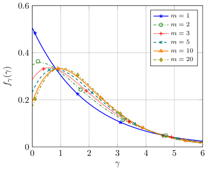
Figure 1: PDF of fSOSF model for different values of $m$. Parameter values are $\alpha=0.1$, $\beta=0.7$ and $\overline{\gamma}_{\rm dB}=3$dB. Theoretical values (10) are represented with lines. Markers correspond to MC simulations.

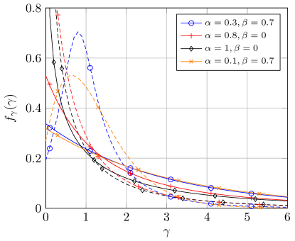
Figure 2: PDF comparison for different values of $\alpha$ and $\beta$. Solid/dashed lines obtained with (10) correspond to ($m=1$, $\overline{\gamma}_{\rm dB}=5$dB) and ($m=20$, $\overline{\gamma}_{\rm dB}=1$dB), respectively. Markers correspond to MC simulations.

In Fig. 1, we represent the PDF of the fSOSF fading model in Lemma 1, for different values of the LoS fluctuation severity parameter $m$. Parameter values are $\alpha=0.1$, $\beta=0.7$ and $\overline{\gamma}_{\rm dB}=3$dB. MC simulations are also included as a sanity check. See that, as we increase the fading severity of the LoS component (i.e., $\downarrow m$), the probability of occurrence of low SNR values increases, as well as the variance of the distribution.

In Fig. 2 we analyze the impact of $\alpha$ and $\beta$ on the PDF of the fSOSF model. Two scenarios have been considered: one with low fading severity and low average SNR ($m=20$, $\overline{\gamma}_{\rm dB}=1dB$), and another with higher fading severity and higher average SNR ($m=1$, $\overline{\gamma}_{\rm dB}=5dB$). In the case of mild fluctuations of the LoS component, the effect of $\beta$ dominates to determine the shape of the distribution, observing a bell-shaped PDFs with higher $\beta$ values. Conversely, the value of $\alpha$ becomes more influential for the left tail of the distribution. We see that lower values of alpha make lower SNR values more likely, which implies an overall larger fading severity.

Finally, we analyze the outage probability (OP) under fSOSF which is defined as the probability that the instantaneous SNR takes a value below a given threshold, $\gamma_{\rm th}$. It can be obtained from the CDF (22) as

$${\rm OP}=F_{\gamma}(\gamma_{\rm th}).$$ (16)

Fig. 3 shows the OP under fSOSF model, for different values of the parameter $m$. Additional parameters are set to $\alpha=0.1$ and $\beta=0.7$, and two threshold values are considered: $\gamma_{\rm th}=3$dB and $\gamma_{\rm th}=1$dB. We see that a $2$dB change in the thresold SNR is translated into a $\sim 5$dB power offset in terms of OP performance. We observe that as the severity of fading increases (i.e., $\downarrow m$), the less likely it is to exceed the threshold value $\gamma_{\rm th}$, i.e., the higher the OP. In all instances, the diversity order (i.e., the down-slope decay of the OP) is one, and the asymptotic OP in (IV) tightly approximates the exact OP, which is given by

$${\rm OP} \left(\alpha,\beta,m;\overline{\gamma},\gamma_{\rm th}\right)\approx\frac{\gamma_{\rm th}}{\alpha\overline{\gamma}}\sum_{j=0}^{m-1}\tbinom{m-1}{j}\left(\tfrac{1-\beta-\alpha}{\alpha}\right)^{m-1-j}\times$$

$$\Gamma(1+j){\rm U}(m,m-j,\tfrac{1}{\alpha}-\tfrac{\beta}{\alpha}\left(\tfrac{m-1}{m}\right)-1).$$ (17)

Expression (IV) can be readily derived by integration over the asymptotic OP of the underlying Rician shadowed model [15, eq. (22)].

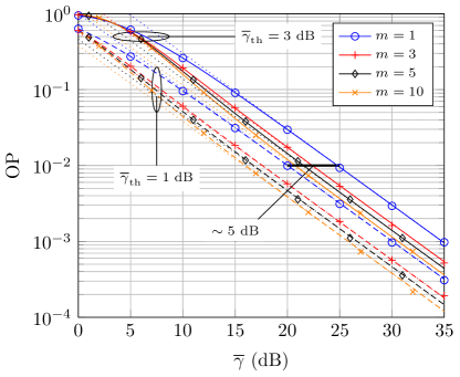
Figure 3: OP as a function of $\overline{\gamma}$, for different values of $m$. Parameter values are $\alpha=0.1$ and $\beta=0.7$. Solid/dashed lines correspond to $\gamma_{\rm th}=3$ and $\gamma_{\rm th}=1$ respectively. Theoretical values (16) are represented with lines. Markers correspond to MC simulations.

V Conclusions

We presented a generalization of Andersen’s SOSF model by incorporating random fluctuations on its dominant specular component, yet without incurring in additional complexity. We provided closed-form expressions for its probability and cumulative distribution functions, as well as for its generalized Laplace-domain statistics and raw moments. Some insights have been provided on how the set of parameters ($\alpha$, $\beta$ and $m$) affect propagation, and its application to performance analysis has been exemplified through an outage probability analysis.

Appendix A Proof of Lemma 1

Noting that $x=|G_{3}|^{2}$ is exponentially distributed with unitary mean, we can compute the distribution of $\gamma$ by averaging over all possible values of $x$ as:

$$f_{\gamma}(\gamma)=\int_{0}^{\infty}f_{\gamma_{x}}(\gamma;x)e^{-x}dx.$$ (18)

The PDF of $\gamma_{x}$ is that of a squared Rician shadowed RV, which for integer $m$ is given by [18, eq. (5)]

$$f_{\gamma_{x}}(\gamma;x)=\sum_{j=0}^{m-1}B_{j}\left(\tfrac{m-j}{\omega_{B}}\right)^{m-j}\tfrac{\gamma^{m-j-1}}{(m-j-1)!}e^{-\frac{\gamma(m-j)}{\omega_{B}}},$$ (19)

where

$$B_{j}=\binom{m-1}{j}\left(\tfrac{m}{K_{x}+m}\right)^{j}\left(\tfrac{K_{x}}{K_{x}+m}\right)^{m-j-1},$$ (20)

$$\omega_{B}=(m-j)\left(\tfrac{K_{x}}{K_{x}+m}\right)\left(\tfrac{\overline{\gamma}_{x}}{1+K_{x}}\right).$$ (21)

with $K_{x}$ and $\bar{\gamma}_{x}$ given in (7) and (8). Substituting (19) into (18), using the change of variables $t=\tfrac{1}{\alpha}\left(1-\beta(\tfrac{m-1}{m})-\alpha(1-x)\right)$ and taking into account that ${(t-\tfrac{\beta}{\alpha m})^{j}=\sum_{r=0}^{j}\binom{j}{r}t^{j}(\tfrac{\beta}{\alpha m})^{j-r}}$, the final expression for the PDF is derived.

Appendix B Proof of Lemma 2

The CDF of the fSOSF model can also be obtained by averaging the CDF of $\gamma_{x}$, i.e., the Rician shadowed CDF over the exponential distribution:

$$F_{\gamma}(\gamma)=\int_{0}^{\infty}F_{\gamma_{x}}(\gamma;x)e^{-x}dx.$$ (22)

For the case of integer $m$, a closed-form expression for the Rician shadowed CDF is presented in [18, eq. (10)], i.e.

$$F_{\gamma_{x}}(\gamma;x)=1-\sum_{j=0}^{m-1}B_{j}e^{\frac{-\gamma(m-j)}{\omega_{B}}}\sum_{r=0}^{m-j-1}\tfrac{1}{r!}\left(\tfrac{\gamma(m-j)}{\omega_{B}}\right)^{r},$$ (23)

Substituting (23) in (22) and following the same approach used in the previous appendix, we obtain the final expression.

Appendix C Proof of Lemma 3

Following the same procedure, the generalized MGF of the fSOSF model denoted as $\mathcal{M}_{\gamma}^{(n)}(s)$ can be obtained by averaging the generalized MGF of $\gamma_{x}$, i.e., the Rician shadowed generalized MGF over the exponential distribution:

$${\color[rgb]{0,0,0}\mathcal{M}_{\gamma}^{(n)}(s)=\int_{0}^{\infty}\mathcal{M}_{\gamma_{x}}^{(n)}(s;x)e^{-x}dx.}$$ (24)

A closed-form expression for $M_{\gamma_{x}}(s;x)$ for integer $m$ is provided in [18, eq. (26)]

$$M_{\gamma_{x}}(s;x)=\frac{m^{m}(1+K_{x})}{\overline{\gamma}_{x}(K_{x}+m)^{m}}\frac{\left(s-\frac{1+K_{x}}{\overline{\gamma}_{x}}\right)^{m-1}}{\left(s-\frac{1+K_{x}}{\overline{\gamma}_{x}}\frac{m}{K_{x}+m}\right)^{m}}$$ (25)

Substituting (7) and (8) into (25) the expression for $M_{\gamma_{x}}(s;x)$ can be rewritten as

$$M_{\gamma_{x}}(s;x)=F_{1}(s;x)\cdot F_{2}(s;x),$$ (26)

where

$$F_{1}(s;x)= -\left[s\bar{\gamma}\left(1-\beta-\alpha(1-x)\right)-1\right]^{m-1},$$ (27)

$$F_{2}(s;x)= \left[s\bar{\gamma}\left(1-\beta\left(\tfrac{m-1}{m}\right)-\alpha(1-x)\right)-1\right]^{-m}.$$ (28)

Next, we compute the $n$-th derivative of (26) wich yields the Rician shadowed generalized MGF

$$\mathcal{M}_{\gamma_{x}}^{(n)}(s;x)=\tfrac{\partial^{n}M_{\gamma_{x}}(s;x)}{\partial s^{n}}=\sum_{q=0}^{n}\tbinom{n}{q}F_{1}^{(n-q)}(s;x)\cdot F_{2}^{(q)}(s;x),$$ (29)

where $F_{i}^{(n)}(s;x)$ denotes the $n$-th derivative of $F_{i}(s;x)$ with respect to $s$.

$$F_{1}^{(n-q)}(s;x)= -(m-n+q)_{n-q}s^{m-1-n+q}(\bar{\gamma}\alpha)^{m-1}\times$$

$$(x+a(s))^{m-1-n+q}(x+c)^{n-q}$$ (30)

$$F_{2}^{(q)}(s;x)= (-1)^{q}(m)_{q}s^{-m-q}(\bar{\gamma}\alpha)^{-m}\times$$

$$(x+b(s))^{-m-q}(x+d)^{q},$$ (31)

where $(z)_{j}$ denotes the Pochhammer symbol and where

$$a(s)= \tfrac{s\bar{\gamma}(1-\beta-\alpha)-1}{s\bar{\gamma}\alpha},$$ (32)

$$b(s)= \tfrac{s\bar{\gamma}\left(1-\beta\left(\tfrac{m-1}{m}\right)-\alpha\right)-1}{s\bar{\gamma}\alpha},$$ (33)

$$c= \tfrac{1-\beta}{\alpha}-1,$$ (34)

$$d= \tfrac{1-\beta\left(\tfrac{m-1}{m}\right)}{\alpha}-1.$$ (35)

From (29), (C) and (C) notice that $\mathcal{M}_{\gamma_{x}}^{(n)}(s;x)$ is a rational function of $x$ with two real positive zeros at $x=c$ and $x=d$, one real positive pole at $x=b(s)$ and one real positive zero or pole at $x=a(s)$ depending on whether $m\geq n+1$ or not. Integration of (24) is feasible with the help of [17, eq. 13.4.4]

$$\int_{0}^{\infty}\frac{x^{i}}{(x+p)^{j}}e^{-x}dx=\Gamma(i+1){\rm U}(j,j-i,p).$$ (36)

where ${\rm U}\left(\cdot,\cdot,\cdot\right)$ is Tricomi’s confluent hypergeometric function [17, (13.1)]. We need to expand $\mathcal{M}_{\gamma_{x}}^{(n)}(s;x)$ in partial fractions of the form $\tfrac{x^{i}}{(x+p)^{j}}$. Two cases must be considered:

• $m\geq n+1$

  In this case there is only one pole at $x=b(s)$ and no partial fraction expansion is required. Using the fact that $(x+p)^{n}=\sum_{i=0}^{n}x^{i}p^{n-i}$, then (3) is obtained.

• $m<n+1$

  Now, there are two poles ($x=a(s)$, $x=b(s)$). After performing partial fraction expansion we obtain (3).

Appendix D Proof of Lemma 4

Using the definition of $\gamma_{x}$, we can write

$$\mathbb{E}[\gamma^{n}]=\int_{0}^{\infty}\mathbb{E}[\gamma_{x}^{n}]e^{-x}dx.$$ (37)

where $\mathbb{E}[\gamma_{x}^{n}]=\lim_{s\rightarrow 0^{-}}M_{\gamma_{x}}^{(n)}(s;x)$ where $M_{\gamma_{x}}^{(n)}(s;x)$ is given in (29). Performing the limit and using the integral $\int_{0}^{\infty}x^{p}e^{-x}dx=p!$, the proof is complete.

References

- [1] P. S. Bithas, K. Maliatsos, and A. G. Kanatas, “The Bivariate Double Rayleigh Distribution for Multichannel Time-Varying Systems,” IEEE Wireless Commun. Lett., vol. 5, no. 5, pp. 524–527, 2016.
- [2] Y. Ai, M. Cheffena, A. Mathur, and H. Lei, “On Physical Layer Security of Double Rayleigh Fading Channels for Vehicular Communications,” IEEE Wireless Commun. Lett., vol. 7, no. 6, pp. 1038–1041, 2018.
- [3] P. S. Bithas, A. G. Kanatas, D. B. da Costa, P. K. Upadhyay, and U. S. Dias, “On the Double-Generalized Gamma Statistics and Their Application to the Performance Analysis of V2V Communications,” IEEE Trans. Commun., vol. 66, no. 1, pp. 448–460, 2018.
- [4] P. S. Bithas, V. Nikolaidis, A. G. Kanatas, and G. K. Karagiannidis, “UAV-to-Ground Communications: Channel Modeling and UAV Selection,” IEEE Trans. Commun., vol. 68, no. 8, pp. 5135–5144, 2020.
- [5] J. K. Devineni and H. S. Dhillon, “Ambient Backscatter Systems: Exact Average Bit Error Rate Under Fading Channels,” IEEE Trans. Green Commun. Netw., vol. 3, no. 1, pp. 11–25, 2019.
- [6] U. Fernandez-Plazaola, L. Moreno-Pozas, F. J. Lopez-Martinez, J. F. Paris, E. Martos-Naya, and J. M. Romero-Jerez, “A Tractable Product Channel Model for Line-of-Sight Scenarios,” IEEE Trans. Wireless Commun., vol. 19, no. 3, pp. 2107–2121, 2020.
- [7] E. Vinogradov, W. Joseph, and C. Oestges, “Measurement-Based Modeling of Time-Variant Fading Statistics in Indoor Peer-to-Peer Scenarios,” IEEE Trans. Antennas Propag., vol. 63, pp. 2252–2263, May 2015.
- [8] V. Nikolaidis, N. Moraitis, P. S. Bithas, and A. G. Kanatas, “Multiple Scattering Modeling for Dual-Polarized MIMO Land Mobile Satellite Channels,” IEEE Trans. Antennas Propag., vol. 66, pp. 5657–5661, Oct 2018.
- [9] J. B. Andersen, “Statistical distributions in mobile communications using multiple scattering,” in Proc. 27th URSI General Assembly, pp. 1–4, 2002.
- [10] J. Salo, H. M. El-Sallabi, and P. Vainikainen, “Statistical Analysis of the Multiple Scattering Radio Channel,” IEEE Trans. Antennas Propag., vol. 54, pp. 3114–3124, Nov 2006.
- [11] J. Lopez-Fernandez and F. J. Lopez-Martinez, “Statistical Characterization of Second-Order Scattering Fading Channels,” IEEE Trans. Veh. Technol., vol. 67, pp. 11345–11353, Dec 2018.
- [12] A. Abdi, W. C. Lau, M. . Alouini, and M. Kaveh, “A new simple model for land mobile satellite channels: first- and second-order statistics,” IEEE Trans. Wireless Commun., vol. 2, no. 3, pp. 519–528, 2003.
- [13] J. F. Paris, “Statistical characterization of kappa-mu shadowed fading,” IEEE Trans. Veh. Technol, vol. 63, pp. 518–526, Feb 2014.
- [14] J. M. Romero-Jerez, F. J. Lopez-Martinez, J. P. Peña-Martín, and A. Abdi, “Stochastic Fading Channel Models With Multiple Dominant Specular Components,” IEEE Trans. Veh. Technol., vol. 71, no. 3, pp. 2229–2239, 2022.
- [15] J. López-Fernández, P. Ramirez-Espinosa, J. M. Romero-Jerez, and F. J. López-Martínez, “A Fluctuating Line-of-Sight Fading Model With Double-Rayleigh Diffuse Scattering,” IEEE Trans. Veh. Technol., vol. 71, no. 1, pp. 1000–1003, 2022.
- [16] M. Chaudhry and S. Zubair, “Generalized incomplete gamma functions with applications,” J Comput Appl Math, vol. 55, no. 1, pp. 99 – 123, 1994.
- [17] “NIST Digital Library of Mathematical Functions.” http://dlmf.nist.gov/, Release 1.0.21 of 2018-12-15. F. W. J. Olver, A. B. Olde Daalhuis, D. W. Lozier, B. I. Schneider, R. F. Boisvert, C. W. Clark, B. R. Miller and B. V. Saunders, eds.
- [18] F. J. Lopez-Martinez, J. F. Paris, and J. M. Romero-Jerez, “The - Shadowed Fading Model with Integer Fading Parameters,” IEEE Trans. Veh. Technol, vol. 66, no. 9, pp. 7653–7662, 2017.