Partial Label Learning for Emotion Recognition from EEG

Abstract

Fully supervised learning has recently achieved promising performance in various electroencephalography (EEG) learning tasks by training on large datasets with ground truth labels. However, labeling EEG data for affective experiments is challenging, as it can be difficult for participants to accurately distinguish between similar emotions, resulting in ambiguous labeling (reporting multiple emotions for one EEG instance). This notion could cause model performance degradation, as the ground truth is hidden within multiple candidate labels. To address this issue, Partial Label Learning (PLL) has been proposed to identify the ground truth from candidate labels during the training phase, and has shown good performance in the computer vision domain. However, PLL methods have not yet been adopted for EEG representation learning or implemented for emotion recognition tasks. In this paper, we adapt and re-implement six state-of-the-art PLL approaches for emotion recognition from EEG on a large emotion dataset (SEED-V, containing five emotion classes). We evaluate the performance of all methods in classical and real-world experiments. The results show that PLL methods can achieve strong results in affective computing from EEG and achieve comparable performance to fully supervised learning. We also investigate the effect of label disambiguation, a key step in many PLL methods. The results show that in most cases, label disambiguation would benefit the model when the candidate labels are generated based on their similarities to the ground truth rather than obeying a uniform distribution. This finding suggests the potential of using label disambiguation-based PLL methods for real-world affective tasks. We make the source code of this paper publicly available at: https://github.com/guangyizhangbci/PLL-Emotion-EEG.

I Introduction

Emotion has been widely recognized as a mental state and a psycho-physiological process that can be associated with various brain or physical activities [1, 2, 3]. It can be expressed through various modalities, such as face expression, hand gestures, body movement, and voice, with various levels of intensity [4]. Emotion plays an important role in our daily life by effecting decision making and interactions [5]; it is thus vital to enable computers to identify, understand, and respond to human emotions [6] for better human-computer interaction and user experience. In recent decades, among non-invasive physiological measurements such as electrocardiography [7], electromyography [8], and electrodermal activity [9], Electroencephalography (EEG) has been widely used for human emotion recognition due to its direct reflection of brain activities [2, 10, 11, 12].

Recently, compared to statistic models and machine learning algorithms, deep learning techniques have grown in popularity, resulting in considerable performance improvements on emotion classification from EEG [10, 13]. Many of the existing deep learning based algorithms are fully supervised, which require annotations for a large amount of training samples [14]. Nonetheless, EEG labeling is a time-consuming, expensive, and difficult process since it requires multiple evaluations such pre-stimulation and post-experiment self-assessment [15, 16, 12]. To tackle the challenge of scarcity of EEG labels, Semi-Supervised Learning (SSL) has been recently explored for emotion recognition using EEG [3, 14, 17].

Another challenge in EEG labeling is the reliability of self-assessment for emotions [18]. For example, after watching emotion-related video clips, participants may find it easy to distinguish between dissimilar emotions or feelings such as ‘happy’ vs. ‘fear’, but have difficulty in distinguishing similar ones, for instance ‘disgust’ vs. ‘fear’. This uncertainty in providing accurate labels may result in an unreliable self-assessment reports [18].

To tackle the above-stated problems, we propose a framework to allow participants to report multiple possible emotions if they are uncertain about their affective state during the self-assessment stage. This notion has been explored in other domains and is referred to as Partial Label Learning (PLL). However, ambiguous labeling often causes performance degradation in deep learning algorithms as the ground truth is hidden within the candidate labels during the training phase [19], making PLL a challenging area. In this paper, we explore several state-of-the-art PLL techniques [20, 21, 22, 23, 24, 19] that have been proposed in the area of computer vision, and adapt them for EEG representation learning for the first time. We use a large-scale emotion EEG dataset, SEED-V [12] and create a new experimental setup to allow for proper testing of PLL techniques with this dataset. We comprehensively compare and analyze these techniques to understand the viability of using PLL for EEG-based emotion recognition. We provide an overview of the core concept behind PLL in Figure 1.

Our contributions in this paper are as follows. (1) For the first time, we address the challenge of ambiguous EEG labeling in emotion recognition tasks. (2) We conduct extensive experiments by re-implementing and adapting six recently developed deep state-of-the-art PLL algorithms for emotion recognition using EEG. (3) We design experiments to evaluate and compare the performance of PLL methods with different candidate labels generation processes. (4) We make our code publicly available at: https://github.com/guangyizhangbci/PLL-Emotion-EEG.

The rest of this paper is organized as follows. In the next section, we provide a literature survey on EEG learning for affective computing followed by an summary of PLL methods proposed in the literature. In Section III, we provide the problem statement and the details of the six PLL techniques which we explore and adopt for EEG. We then describe the dataset in Section IV, along with implementation details and experiment setup. In Section V, the detailed results and analysis are provided. And finally Section VI presents the concluding remarks.

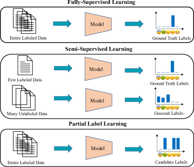
Figure 1: A description of full-supervised learning, semi-supervised learning and partial label learning for emotion recognition is presented.

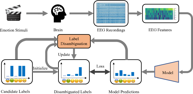
Figure 2: A general EEG-based PLL framework for emotion recognition is presented.

II Background

II-A Deep EEG Representation Learning

Deep learning techniques, such as deep belief networks [15], fully connected neural networks [10], Convolutional Neural Networks (CNNs) [25], capsule networks [26, 11], Recurrent Neural Networks (RNNs)[27], long short-term networks [28], graph neural networks [29, 30], as well as combinations of CNNs and RNNs [31] have been widely used for EEG-based fully-supervised tasks, such as motor imagery or movement classification and emotion recognition [32, 33]. These deep learning techniques outperformed classical statistics algorithms and conventional machine learning methods in most tasks, as they are able to learn non-linear and more complex patterns, and focus on task-relevant features [28, 10, 26]. CNNs are the most popular deep learning backbones for EEG learning [32, 33, 25].

Deep EEG representation learning frameworks have also shown good performance in semi-supervised tasks, where only a few EEG annotations are available during training [3, 14]. An attention-based recurrent autoencoder was proposed for semi-supervised EEG learning [3]. Furthermore, state-of-the-art semi-supervised techniques originally developed for computer vision tasks, such as MixMatch [34], FixMatch [34] and AdaMatch [35], have been adapted for EEG learning and obtained promising results in emotion recognition tasks. A novel pairwise EEG representation alignment method (PARSE), based on a lightweight CNN backbone, was lately proposed and achieved state-of-the-art results in semi-supervised tasks on multiple publicly available large-scale affective datasets [17]. More importantly, PARSE achieved similar performance to fully-supervised models trained on large-scale labeled datasets with substantially fewer labeled samples, demonstrating the superiority of deep semi-supervised EEG learning in the face of a scarcity of labeled data [17].

II-B Partial Label Learning

PLL algorithms have been lately used to tackle the challenges of label ambiguity and achieved promising performance in a variety of image classification tasks with ambiguous labels. For instance, in [20], a deep naive partial label learning model was proposed based on the assumption that distribution of candidate labels should be uniform since ground truth is unknown [36]. In addition to this naive approach, a number of other frameworks have been lately developed to rely on a process called ‘label disambiguation’, which refines the distribution of candidate labels by updating it in each training iteration. This process of combining label disambiguation and model classification works as an Expectation-Maximization (EM) algorithm as shown in [36]. Specifically, the candidate labels’ distribution is initially assumed to be uniform. In the first iteration, a model is trained on the uniformly distributed candidate labels. Then, the candidate labels are disambiguated based on the trained model’s predictions. In the next iteration, the model is trained on the disambiguated candidate labels, and the process repeats during the training phase [36, 21].

In [22], a method was proposed for label disambiguation that utilized the importance of each output class, rather than relying solely on the model’s predictions. To mitigate the possible negative effect of training on false positive labels, in [23, 24], a method was proposed to leverage both candidate and non-candidate labels with the label disambiguation process. Furthermore, in [19], a prototype-based label disambiguation method was proposed, which was used in combination with supervised contrastive learning [37], a technique that relies on contrastive loss to train a Siamese-style network. Specifically, first, prototype-based label disambiguation is used to guess the ground truth and generate accurate positive pairs for contrastive learning. Then, the contrastively learned embeddings, in turn, could better guide the label disambiguation process. Thus, these two components are mutually beneficial during the iterative training, leading the PLL framework to achieve state-of-the-art results in multiple vision tasks [19].

III PLL Methods

III-A Problem Setup

Let’s denote $\mathcal{X}$ and $\mathcal{Y}\in\{1,2,...k\}$ as the input EEG feature space and the emotion label space, respectively, where $k$ is the total number of emotion categories. Accordingly, $x\in\mathcal{X}$ and $y\in\mathcal{Y}$ represent EEG samples and emotion ground truth labels. For a classification problem with ambiguous labels, the collection of all subsets in $\{1,2,...k\}$, $2^{\mathcal{Y}}\setminus\emptyset$ has been used instead of $\mathcal{Y}$ as the label pace. The training set $D=\{(x_{i},Y_{i})\}_{i=1}^{N}$ consists of normalized EEG input $x_{i}\sim[0,1]$, and candidate label $Y_{i}\subset 2^{\mathcal{Y}}\setminus\emptyset$. The ground truth $y_{i}$ is concealed in the candidate labels as $y_{i}\in Y_{i}$.

In classical PLL literature, candidate labels are assumed to be generated independently, uniformly, and randomly. Thus, for the distribution of each candidate label set, we have $\mathrm{P}(Y_{i}\mid x_{i},y_{i},q)=\prod_{s\neq y_{i}}q,\forall s\in[1,k]$, where $q<1$ represents the degree of label ambiguity. Note that $q=1\iff s=y_{i}$. The goal of PLL is to construct a robust multi-class classifier by minimizing the divergence between model output and candidate labels. In this study, we aim to evaluate the effectiveness of various PLL algorithms for EEG representation learning when emotion labels with different levels of ambiguity are provided.

III-B Method Overview

A general PLL framework for emotion recognition is illustrated in Figure 2. In a typical EEG-based emotion recognition experiment setup, EEG recordings are collected from a participant’s brain scalp while they are watching an emotion-related video clip. Then, candidate labels are generated based on the participant’s self-assessment. These candidate labels are then used to train a model with the features extracted from EEG recordings. The label disambiguation is often based on uniformly distributed candidate labels ($\hat{Y}$) or the disambiguated labels obtained from last training iteration ($\vec{Y}$) and model predictions ($p_{m}(x)$). The disambiguated labels ($\vec{Y}$) are updated in each training iteration, and the model is trained by minimizing divergence between the model predictions and the disambiguated labels. When label disambiguation is not used, the divergence will be consistently minimized between model predictions and the candidate labels (with uniform distribution) during the entire training phase. Training is performed by batches, where $x_{b}$ denotes input samples of each batch.

We identify six state-of-the-art PLL techniques from the literature, which re-implement and adapt for emotion recognition from EEG. These methods are Deep Naive Partial Label (DNPL) learning [20], PROgressive iDENtification (PRODEN) true Labels for PLL [21], Class Activation Value Learning (CAVL) for PLL, [22], Leveraged Weighted (LW) loss for PLL [23], revisiting Consistency Regularization (CR) [24] for deep PLL, and Partial label learning with COntrastive label disambiguation (PiCO) [19], which we describe in the following sub-sections.

III-C DNPL

In DNPL [20], since the ground truth is unknown [36], the candidate labels are assumed to have uniform distribution as follows:

$$\overline{\hat{Y}_{s}}=\frac{1}{|Y|}\leavevmode\nobreak\ \leavevmode\nobreak\ \leavevmode\nobreak\ \leavevmode\nobreak\ \text{if}\leavevmode\nobreak\ \leavevmode\nobreak\ s\in Y,\leavevmode\nobreak\ \leavevmode\nobreak\ \leavevmode\nobreak\ 0\leavevmode\nobreak\ \leavevmode\nobreak\ \text{otherwise},$$ (1)

where $\hat{Y}_{s}=1,\forall s\in Y$. The DNPL model is simply trained by minimizing the divergence between the model’s predictions and the uniformly distributed candidate labels, as:

$$\mathcal{L}_{naive}=-\frac{1}{|x_{b}|}\sum_{i=1}^{|x_{b}|}\log(\nu(\hat{Y}\phi(p_{m}(x_{i})))),$$ (2)

where $\phi(.)$ denotes the softmax operation, and $\nu$ is the clamp operator which limits the output in the range of $[0,1]$.

III-D PRODEN

PRODEN was proposed to refine candidate labels through a label disambiguation process [21]. Specifically, the process obtains disambiguated labels by multiplying model predictions with candidate labels, as: $\vec{Y}=p_{m}(x)\hat{Y}$. Following, the model is trained by minimizing cross-entropy between the model’s predictions and the disambiguated labels, as:

$$\mathcal{L}_{ce}=-\frac{1}{|x_{b}|}\sum_{i=1}^{|x_{b}|}\vec{Y}\leavevmode\nobreak\ \log(\phi(p_{m}(x_{i}))).$$ (3)

Here, when the label disambiguation process is not used, $\vec{Y}$ will be replaced by $\hat{Y}$.

III-E CAVL

In [22], CAVL was proposed to disambiguate candidate labels by focusing on the importance score of each label in the model’s predictions. Specifically, inspired by [38], CAVL uses gradient flow ($v^{s}$) of the network output’s log probability as a measurement of the importance of each label, which is shown as:

$$\begin{split}v^{s}&=\bigg{|}\frac{\partial(-\log(\phi^{s}(p_{m}(x))))}{\partial p_{m}(x)}\bigg{|}\partial\phi^{s}(p_{m}(x))\\ &=\big{|}\phi^{s}(p_{m}(x))-1\big{|}\phi^{s}(p_{m}(x)),\forall s\in[1,k].\end{split}$$ (4)

As suggested in [22], $\phi(p_{m}(x))$ is replaced by $p_{m}(x)$ since $p_{m}(x)$ contains more information. Consequently, we have $\hat{v}^{s}=\big{|}p_{m}^{s}(x_{i})-1\big{|}p_{m}^{s}(x_{i})$ and disambiguated label $\vec{Y}=\operatorname*{arg\,max}(\hat{v}^{s}\overline{\hat{Y}})$. The same cross-entropy loss in (Eq. 3) is used for model training. When label disambiguation is not used, same as in PRODEN, $\vec{Y}$ will be replaced by $\hat{Y}$.

III-F LW

Most existing PLL algorithms only focus on learning from candidate labels while ignoring non-candidate ones [20, 21, 22, 19]. However, a model could be misled by the false positive labels if it only relies on the candidate label set [24]. To mitigate this possible negative effect, in [23], both candidate and non-candidate labels have been used for model training using a LW loss. To do so, first, the sigmoid loss $\sum_{s\notin Y}\varphi(p_{m}(x))$ ($\varphi(.)$ representing sigmoid operation) or negative log-likelihood loss $-\sum_{s\notin Y}\log(1-\phi(p_{m}(x)))$ is applied on non-candidate labels, in order to discourage the model predictions to be among the non-candidate labels. Next, the modified sigmoid loss $\sum_{s\in Y}\varphi(-p_{m}(x))$ or negative log-likelihood loss $-\sum_{s\in Y}\log(\phi(p_{m}(x)))$ is employed for model training on candidate labels. Finally, the model is trained on both candidate and non-candidate labels. The total loss function using the sigmoid function and cross-entropy loss (negative log-likelihood) is shown in Eq. 5 and Eq. 6, respectively.

$$\mathcal{L}_{ce}^{lw}=-\frac{1}{|x_{b}|}\sum_{i=1}^{|x_{b}|}\big{[}\sum_{s\in Y}w_{s}\varphi(-p_{m}(x_{i}))+\beta\sum_{s\notin Y}w_{s}\varphi(p_{m}(x_{i}))\big{]},$$ (5)

$$\begin{split}\mathcal{L}_{sig}^{lw}&=-\frac{1}{|x_{b}|}\sum_{i=1}^{|x_{b}|}\big{[}\sum_{s\in Y}w_{s}\log(\phi(p_{m}(x_{i})))\\ &+\beta\sum_{s\notin Y}w_{s}\log(1-\phi(p_{m}(x_{i})))\big{]}.\end{split}$$ (6)

A trade-off parameter $\beta=0,1,2$ is applied as suggested in [23]. The weights $w_{s}$ are the normalized model predictions, as $w_{s}=\phi(p_{m}(x_{i})),\forall s\in Y$ and $w_{s}=\phi(p_{m}(x_{i})),\forall s\notin Y$. The wights ($w_{s}$) are updated chronologically and used to assign more weights to learn the candidate labels which are more likely to be the ground truth and the more confusing non-candidate labels. Note that $w_{s}=1$ when label disambiguation is not used.

III-G CR

In [24], both candidate and non-candidate labels are leveraged in a similar manner to the LW method [23], where modified negative log-likelihood loss is applied on non-candidate labels, as $\mathcal{L}_{s}=-\frac{1}{|x_{b}|}\sum_{i=1}^{|x_{b}|}\sum_{s\notin Y}\log(1-\phi(p_{m}(x_{i})))$. In [24], instead of using cross-entropy loss, a consistency regularization method has been proposed for learning candidate labels. Consistency regularization encourages a model to have consistent predictions on the original data or its perturbed versions [39, 34, 17]. As suggested in [24], consistency regularization is applied by minimizing the divergence between each augmentation of an instance and its refined label. To do so, we first obtain the refined label based on the network predictions of the original data and its different augmentations, as:

$$\vec{Y}_{s}=\prod_{i=1}^{3}\phi(p_{m}(A_{i}(x_{b})))^{1/3},\forall s\in Y$$ (7)

where $A_{i}$ presents the original, weakly, and strongly augmented data, as $x,A_{w},A_{s}$ when $i=1,2,3$. Additive Gaussian noise has been commonly used as an effective data augmentation method in recent EEG studies [40, 41, 14, 17]. Therefore, we produce the augmented data as $\mathcal{A}_{s/w}(x)=x+\mathcal{N}(\mu,\sigma)$, where $\mathcal{N}$ represents a Gaussian distribution. As suggested in [26, 17], we choose mean value ($\mu$) of $0.5$, and standard deviation values ($\sigma$) of $0.8$ and $0.2$ for strong ($\mathcal{A}_{s}$) and weak ($\mathcal{A}_{w}$) augmentations respectively. Following, we minimize the divergence between different augmentations of an instance and its refined label,

$$\mathcal{L}_{u}=\frac{1}{|x_{b}|}\sum_{i=1}^{|x_{b}|}\sum_{j=1}^{3}D_{KL}(\vec{Y}^{\prime}||\log(\phi(p_{m}(A_{j}(x_{i}))))),$$ (8)

where $D_{KL}$ denotes Kullback-Leibler (KL) divergence and $\vec{Y}^{\prime}$ denotes the normalized disambiguated labels, as $\vec{Y}^{\prime}=\vec{Y}/\sum_{s\in Y}\vec{Y}$. Finally, the total loss consists of a supervised loss applied on non-candidate labels and a consistency regularization term applied on candidate labels,

$$\mathcal{L}^{cr}=\mathcal{L}_{s}+\eta\mathcal{L}_{u},$$ (9)

where $\eta=t/T$ is the warm-up function. $t$ and $T$ represent current epoch and the total training epochs, respectively. We have $\eta=0$ when label disambiguation is not used.

III-H PiCO

PiCO was proposed to incorporate contrastive learning and a prototype-based label disambiguation method for effective partial label learning [19]. PiCO employs a similar framework with MoCo [42], which includes a query network $p_{m}$ and a key network $p^{\prime}_{m}$ sharing the same encoder architecture, where $p^{\prime}_{m}$ uses a momentum update with $p_{m}$ [42]. Following we describe the details of the contrastive learning and the prototype-based label disambiguation technique.

Contrastive Learning. Contrastive learning has achieved promising performance in both supervised and unsupervised learning tasks by maximizing the similarity between learned representations of a positive pair [37, 43, 42]. In the supervised contrastive learning, a positive pair includes samples from the same class, while a negative pair contains examples belonging to different classes. In unsupervised contrastive learning, a positive pair often consists of a sample and its augmentation, while a negative pair consists of a sample and a randomly chosen instance.

Since the ground truth is unknown in partial label learning tasks, contrastive learning could be performed in an unsupervised manner. To do so, we first construct a positive pair using an instance ($x_{i}$) and its weak augmentation ($A_{w}(x_{i})$). Then, we obtain a pair of L$2$ normalized embeddings from the query and key networks, as $Q_{i}=||p_{\operatorname{emb}}(x_{i})||_{2}$, $K_{i}=||p^{\prime}_{\operatorname{emb}}(A_{w}(x_{i}))||_{2}\in(0,1)^{N_{\operatorname{emb}}}$, where $p_{\operatorname{emb}}$ and $p^{\prime}_{\operatorname{emb}}$ denotes the embeddings obtained from encoders $p_{m}$ and $p^{\prime}_{m}$, respectively. $N_{\operatorname{emb}}=64$ denotes the dimension of the embeddings. Following, we initialize the negative sample pool as $\operatorname{queue}\in\mathbb{R}^{[N_{q}\times k]},\text{where}\operatorname{queue}_{i,j}\sim\mathcal{N}(0,1),\forall i\in[1,N_{q}],\forall j\in[1,N_{\operatorname{emb}}]$, as suggested in [42]. We set the length of the pool, $N_{q}=1000$, according to the total number of EEG training samples. Next, we calculate the unsupervised contrastive loss as:

$$\mathcal{L}_{u}^{ct}=-\frac{1}{|x_{b}|}\sum_{i=1}^{|x_{b}|}\log\frac{\exp((\operatorname{bmm}(Q_{i},K_{i})/\tau)}{\sum_{i=1}^{|x_{b}|}\sum_{1}^{N_{q}}\exp(Q_{i}\operatorname{queue}^{\top}/\tau)},$$ (10)

where $\operatorname{bmm}$ denotes the batch matrix multiplication operator such that $\operatorname{bmm}(Q_{i},K_{i})\in\mathbb{R}^{[|x_{b}|,1]}$. We choose the temperature hyper-parameter $\tau=0.07$, as suggested in [19].

Unsupervised contrastive learning remains challenging since the false negative samples in the negative samples pool may cause performance degradation [37, 44]. To tackle this challenge, one solution is to construct a positive pair consisting of two samples whose guessed labels are the same. To do so, we first estimate the pseudo-label as $\vec{Y}_{i}=\phi{(p_{m}(x_{i}))}\overline{\hat{Y}_{i}}$. We then construct the contrastive representation pool as $\operatorname{queue}^{+}=\operatorname{cat}(K,\operatorname{queue})$, where cat$(.)$ denotes a concatenation operation. We also have the corresponding pseudo-label pool as ${Y^{\operatorname{queue}^{+}}=\operatorname{cat}(\overline{\hat{Y}},Y^{\operatorname{queue}})}$, where $Y^{\operatorname{queue}}\sim\mathcal{N}(0,1)$. Next, we construct the set of instances with the same guessed label as $S_{\operatorname{pos}}=\{V^{\prime}|V^{\prime}\in\operatorname{queue}^{+},\operatorname*{arg\,max}(Y^{\operatorname{queue}^{+}}_{j})=\operatorname*{arg\,max}(\vec{Y}_{i}),\forall i\in[1,|x_{b}|],\forall j\in[1,N_{q+}]\}$, where $N_{q+}$ represents the length of $\operatorname{queue}+$. Following, we employ the supervised contrastive loss as:

$$\small\mathcal{L}_{s}^{ct}=-\frac{1}{|x_{b}|}\sum_{i=1}^{|x_{b}|}\{\frac{1}{|S_{\operatorname{pos}}|}\sum_{V^{\prime}\in{S_{\operatorname{pos}}}}\log\frac{\exp(Q_{i}V^{\prime\top}/\tau)}{\sum_{V\in{\operatorname{queue}^{+}}}\exp(Q_{i}V^{\top}/\tau)}\}.$$ (11)

Both the negative samples pool and the corresponding pseudo-label pool, are randomly initialized with Gaussian distributions. $\operatorname{queue}$ is replaced by the embeddings $K$ obtained in the previous training batch, and $Y^{\operatorname{queue}}$ is replaced by the uniformly distributed candidate labels $\overline{\hat{Y}}$, chronologically.

Prototype-based Label Disambiguation. Prototype is defined as a representative embedding of instances with the same label [45, 19]. We denote prototype as $\operatorname{proto}\in\mathbb{R}^{k\times N_{\operatorname{emb}}}$, where the instances belonging to each class have their unique embedding vector. From an EM perspective, the E-step uses clustering to estimate the distribution of the prototype, and the M-step is to update the query network parameters through contrastive learning [45, 19]. The prototype is zero initialized and smoothly updated by the embedding $Q$ as:

$$\begin{split}\operatorname{proto}_{j}&=||\operatorname{proto}_{j}*\lambda+(1-\lambda)*Q_{i}||_{2},\\ &\text{if}\leavevmode\nobreak\ j=\operatorname*{arg\,max}(\overline{\hat{Y}}\phi(p_{m}(x_{i}))),\forall i\in[1,|x_{b}|],\forall j\in[1,k],\end{split}$$ (12)

where $\lambda=0.99$ is the coefficient used in a moving average strategy. Following, the pseudo-label after prototype-based disambiguation is denoted as:

$$Y^{\operatorname{proto}}_{i}=\operatorname*{arg\,max}(\phi(Q_{i}\operatorname{proto}^{\top})\overline{\hat{Y_{i}}}).$$ (13)

Finally, the total loss consists of the cross-entropy loss and the supervised contrastive loss using prototype-disambiguated labels, as

$$\mathcal{L}=\mathcal{L}_{ce}+\xi\mathcal{L}_{s}^{cont},$$ (14)

where $\vec{Y}$ refers to $Y^{\operatorname{proto}}$. We adopt $\xi=0.5$ as the contrastive loss weight, as suggested in [19]. When the label disambiguation process is not used, the contrastive loss $\mathcal{L}_{s}^{ct}$ will be replaced by $\mathcal{L}_{u}^{ct}$, and $\vec{Y}$ will be replaced by $\hat{Y}$ in Eq. 3. Note that when contrastive learning is not used, $\xi=0$.

IV Experiment Setup

IV-A Dataset

We use the SEED-V dataset [12] to evaluate and compare the different techniques described earlier. In this dataset, $45$ short films with five emotions (happy, neutral, sad, fear, and disgust) were used as stimuli. $16$ participants including $10$ females and $6$ males participated in the study. All participants repeated the experiment three times, with completely new stimuli each time. Each experiment contains $3$ trials for each emotion, yielding $15$ trials in total. Each trial includes three stages: $15$ seconds initial stimuli prior to starting, $2-4$ minutes of watching film clips, and $15$ or $30$ seconds of self-assessment on the induction effect of the stimuli. EEG recordings were collected with $62$ channels at a sampling frequency of $1000$Hz.

IV-B Feature Space

EEG recordings in each experiment were split into continuous and non-overlapping $4$-second segments. We use the same Differential Entropy (DE) features provided by the dataset [12]. DE features were extracted from $5$ EEG bands (delta, theta, alpha, beta, and gamma) and all $62$ EEG channels for each segment, yielding $s=310$ features in total. We normalize the feature vector of each segment ($x_{i}\sim[0,1]^{310}$) to be used as input for training the models.

IV-C Evaluation Protocols

We apply the same evaluation protocols that were originally used in [12]. Specifically, EEG recordings of each subject have been formed into three pre-defined folds. Fold No. 1 includes the first $5$ trials of all three repeated experiments, yielding $15$ trials in total. A similar strategy is applied to folds No. $2$ and $3$. Next, a 3-fold cross-validation scheme has been used for training and testing, as suggested in [12].

IV-D Backbone Model

We employ the same lightweight CNN used in very recent EEG-based affective computing studies [14, 17] as the backbone model. As shown in Table I, the encoder consists of two 1-dimensional (1-D) convolutional blocks. Each block has a 1-D convolutional layer followed by a 1-D batch normalization layer and a LeakyReLU activation function. The encoder is used to transform the input EEG data into a compact representation. The learned embedding is then fed to the classifier which includes two fully connected layers with a dropout rate of 0.5 for emotion recognition. In the table, $s$ and $k$ denote the total number of EEG features, and the number of emotion categories, respectively.

Table I: Backbone Model Details.

Module	Layer details	Output shape
Input	-	$(1,s)$
Encoder	$\begin{bmatrix}\text{Conv1D},\text{kernel}(3),\text{output channels}(5)\\ \text{BatchNorm1D},\text{output channels}(5)\\ \text{LeakyReLU},\text{slope(0.3)}\ \end{bmatrix}$	$(5,s-2)$
	$\begin{bmatrix}\text{Conv1D},\text{kernel}(3),\text{output channels}(10)\\ \text{BatchNorm1D},\text{output channels}(10)\\ \text{LeakyReLU},\text{slope(0.3)}\ \end{bmatrix}$	$(10,s-4)$
Embedding	Flatten	$10\times(s-4)$
Classifier	$\begin{bmatrix}\text{Linear},64\\ \text{ReLU},-\\ \text{Dropout},0.5\\ \text{Linear},k\ \end{bmatrix}$	$(k)$

IV-E Implementation Details

In all the experiments, we ran $T=30$ training epochs with a batch size of $|x_{b}|=8$. We set the learning rate to $0.01$ and used SGD as the optimizer with a default momentum of $0.9$ and weight decay of $0.0001$. The learning rate scheduler was not used for the naive method [20] and the fully supervised method as it hurt the performance in these cases. All the PLL methods have been evaluated five times, each time with different random seeds used for candidate label generation. Our experiments were carried out on two NVIDIA GeForce RTX $2080$ Ti GPUs using PyTorch [46]. For the sake of reproducibility, we made the source code of this work publicly available at: https://github.com/guangyizhangbci/PLL-Emotion-EEG.

Table II: The accuracy (in %) of Comparison PLL Methods.

Method	Venue	LD	$q=0.2$	$q=0.4$	$q=0.6$	$q=0.8$	$q=0.9$	$q=0.95$
Fully Supervised	-	-	63.08 (13.87)
PRODEN [21]	ICML20	✗	58.55(16.63)	57.69(15.99)	53.87(15.24)	43.05(14.76)	32.37(11.73)	26.00(10.72)
		✓	59.73(16.81)	58.83(16.12)	55.87(16.37)	47.53(14.06)	37.58(13.54)	26.99(10.32)
DNPL [20]	ICASSP21	✗	60.86(16.64)	60.37(15.82)	59.62(16.45)	59.42(15.65)	57.08(16.46)	49.44(15.85)
LW [23]	ICML21	✗	60.64(15.83)	58.86(16.03)	55.97(15.91)	48.43(14.00)	36.09(12.14)	29.30(11.57)
		✓	60.48(16.75)	60.83(16.22)	59.81(16.30)	54.61(16.30)	34.35(17.91)	22.12(10.33)
CAVL [22]	ICLR22	✗	58.51(16.63)	57.60(15.90)	53.67(15.24)	43.03(14.70)	32.39(11.66)	26.03(10.68)
		✓	57.58(16.52)	54.94(16.68)	48.58(15.64)	30.75(12.18)	23.44 (8.19)	21.72 (7.03)
CR [24]	ICML22	✗	42.42(13.70)	42.64(14.37)	41.22(13.56)	35.60(12.62)	30.70(10.71)	26.41 (9.27)
		✓	28.31(10.08)	28.55 (9.52)	27.57 (9.57)	22.68 (8.66)	22.09 (7.90)	20.94 (8.56)
PiCO [19]	ICLR22	✗	57.23(16.44)	55.28(16.71)	49.95(15.89)	38.04(12.82)	28.34(11.18)	24.91(10.26)
		✓	62.68(15.88)	61.92(15.94)	57.54(15.59)	43.87(14.99)	31.26(11.52)	24.69 (9.66)

Table III: The accuracy (in %) of LW [23] with different settings.

Method	$\beta$	LD	$q=0.2$	$q=0.4$	$q=0.6$	$q=0.8$	$q=0.9$	$q=0.95$
LW-Sigmoid	0	✗	35.68(12.69)	31.25(11.01)	26.79(10.01)	22.14 (9.22)	22.47 (9.26)	20.66 (8.84)
		✓	30.14(10.52)	27.88(10.03)	23.03 (8.03)	20.98 (6.79)	20.11 (6.52)	20.00 (6.65)
	1	✗	57.44(16.66)	48.55(15.32)	34.54(11.24)	25.77 (9.85)	24.35 (9.68)	22.08 (9.62)
		✓	40.99(23.27)	33.97(19.67)	24.74(10.24)	20.75 (7.80)	20.04 (6.99)	20.61 (6.72)
	2	✗	36.72(15.55)	48.96(18.35)	49.51(15.64)	28.98(11.12)	24.54 (9.70)	22.52 (9.40)
		✓	42.44(23.89)	37.82(22.15)	32.85(19.30)	21.56 (9.26)	20.25 (6.91)	20.53 (7.35)
LW-Cross Entropy	0	✗	59.44(16.16)	57.17(16.03)	53.93(15.14)	42.63(14.17)	31.81(12.40)	27.29(11.04)
		✓	59.71(16.81)	58.85(16.08)	55.73(16.23)	48.13(13.88)	36.83(13.21)	27.81(10.48)
	1	✗	60.14(15.85)	58.49(16.13)	55.58(15.96)	46.38(14.55)	33.95(12.81)	28.27(11.14)
		✓	60.23(16.84)	60.01(16.36)	58.79(16.14)	51.48(16.19)	30.47(15.87)	22.05(10.25)
	2	✗	60.64(15.83)	58.86(16.03)	55.97(15.91)	48.43(14.00)	36.09(12.14)	29.30(11.57)
		✓	60.48(16.75)	60.83(16.22)	59.81(16.30)	54.61(16.30)	34.35(17.91)	22.12(10.33)

Table IV: The accuracy (in %) of PiCO [19] with different settings.

CL	LD	$q=0.2$	$q=0.4$	$q=0.6$	$q=0.8$	$q=0.9$	$q=0.95$
✗	✗	59.35(16.09)	57.75(16.27)	53.13(15.84)	43.31(13.41)	33.30(12.53)	27.12(10.52)
✗	✓	59.48(16.27)	58.77(16.65)	55.21(16.52)	45.93(16.42)	35.12(13.51)	25.81 (9.60)
✓	✗	57.23(16.44)	55.28(16.71)	49.95(15.89)	38.04(12.82)	28.34(11.18)	24.91(10.26)
✓	✓	62.68(15.88)	61.92(15.94)	57.54(15.59)	43.87(14.99)	31.26(11.52)	24.69 (9.66)

V Results

V-A Performance in Classical Experiments

We evaluate the performance of each PLL method in all $6$ scenarios with different levels of ambiguity ($q\in\{0.2,0.4,0.6,0.8,0.9,0.95\}$) and present the results in Table II. We observe that when low ambiguous candidate labels ($q\in\{0.2,0.4\}$) are provided, PiCO [19] obtains the best results (shown in bold). DNPL [20] obtains the second-best performance (shown with underline) with less ambiguous labels ($q\in\{0.2,0.6\}$) while achieving the best performance with more ambiguous labels ($q\in\{0.8,0.9,0.95\}$). LW method [23] obtains the best and the second-best results when the label ambiguity is moderate ($q\in\{0.4,0.6,0.8\}$). Overall, across all the scenarios, DNPL [20] maintains a very stable performance, while others suffer from major performance drops when candidate labels are provided with very high ambiguity ($q>0.8$).

All PLL methods use label disambiguation methods except for DNPL [20]. To analyze the effect of label disambiguation in each PLL methods, we evaluate the majority of PLL methods both with and without Label Disambiguation (LD). As shown in Table II, among these five PLL methods, LD methods play different roles. Specifically, LD consistently improves the model performance in PRODEN [21] and PiCO [19] (except when $q=0.95$), while causing performance decline in CAVL [22] and CR [24], across all the ambiguously labeled scenarios. In LW method [23], LD is able to improve the model performance when candidate labels with lower ambiguity are provided ($q\in\{0.4,0.6,0.8\}$). However, when candidate labels are provided with very high ambiguity ($q\in\{0.9,0.95\}$), LD results in performance degradation.

Furthermore, we compare the average performance (across $q\in\{0.2,0.4,0.6,0.8,0.9,0.95\}$) for all the PLL methods. As illustrated in Figure 3, DNPL shows the best performance, followed by LW, when label disambiguation is not used. With label disambiguation, LW outperforms the rest, followed by PRODEN. We also observe that label disambiguation methods do not improve the model performance in CAVL [22] and CR [24], while in LW [23], the average performance stays almost the same with and without label disambiguation.

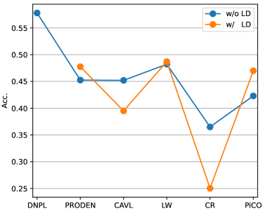
Figure 3: Average performance of all PLL methods across all $6$ ambiguously labeled scenarios ($q\in\{0.2,0.4,0.6,0.8,0.9,0.95\}$).

In LW [23], we further evaluate the method using both sigmoid and cross-entropy losses with three suggested values for the loss leveraging parameter ($\beta=0,1,2$) (discussed in section III-F). This experiment is performed as these parameters are deemed important in the original LW paper [23]. As shown in Table III, LW with cross-entropy loss outperforms LW with sigmoid loss in all the $\beta$ and LD settings, across all the ambiguously labeled scenarios. LW with cross-entropy loss achieves the best results when more weights are assigned for learning non-candidate labels ($\beta=2$).

In PiCO [19], we evaluate the impact of two major components, namely Contrastive Learning (CL) and label disambiguation (discussed in section III-H). As shown in Table IV, we find that CL and LD are beneficial in cases where the candidate labels are less ambiguous ($q\in\{0.2,0.4,0.6\}$). PiCO performs the best without CL when label ambiguity increases ($q\in\{0.8,0.9\}$), and obtains the top performance without both components when label ambiguity is very high ($q=0.95$).

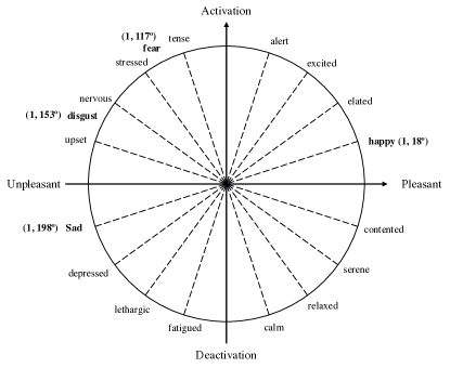
Figure 4: Wheel of emotions reproduced from [47, 48].

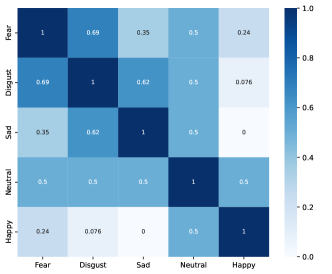
Figure 5: Estimation of normalized similarity score between two emotions.

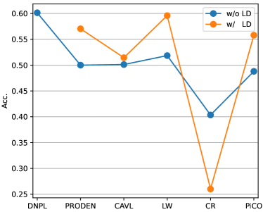
Figure 6: Performance of all PLL methods in the real-world experiments

V-B Performance in Real-World Scenarios

Most existing PLL methods employ independent sampling for candidate label generation, where each class except for the ground truth has the same probability of $q$ to become the candidate label. However, independent sampling may not be suitable for emotion recognition tasks since in the real word scenarios, it is more likely to confuse emotions that are more closely related (e.g., ‘sad’ and ‘fear’), while it is less likely to confuse dissimilar emotions (e.g., ‘sad’ and ‘happy’). To address this, we design additional experiments to generate the candidate labels based on the similarity between two emotions. To do so, we first estimate the location of each emotion on Russell’s circumplex model [47, 48]. As shown in Figure 4, the wheel of emotions is a circumplex that represents the relationships between different emotions on two orthogonal axis, arousal and valence. This was first proposed by Russell [47] and further developed in studies such as [48]. In this model, emotions are arranged in a circular layout, with certain emotions being considered more closely related to one another based on their proximity on the wheel. To perform more realistic experiments on label generation, we estimate the polar coordinates of each emotion in the format of (radius, angle degrees). According to [48], we assume that emotions (with the exception of disgust and fear) are uniformly distributed in each quarter of the wheel, with each adjacent angle representing a difference of $18^{\circ}$. ‘Disgust’ is positioned between ‘upset’ and ‘nervous’, and ‘fear’ is positioned between ‘stressed’ and ‘tense’. Moreover, the ‘neutral’ emotion is always placed at the center of the wheel, at the coordinate of $(0,0^{\circ})$. Based on this distribution, we can determine the polar coordinates of each emotion, with the radius of the wheel being set to $1$. Following, we calculate the distance between two emotions ($i$ and $j$), as $\operatorname{dist}(i,j)=\sqrt{r_{i}^{2}+r_{j}^{2}-2r_{i}r_{j}\cos{(\theta_{i}-\theta_{j})}}$, where $r$ and $\theta$ denote the radius and angle radians, respectively. Next, we obtain the normalized similarity score between two emotions, as $\gamma(i,j)=1-\operatorname{dist}(i,j)/\max{(\operatorname{dist}(i,j))},\forall i,j\in[1,k]$. The normalized similarity scores among the five emotions are shown in Figure 5. Finally, for candidate label generation, we use the normalized similarity score instead of a pre-defined constant ($q$) as the probability, such that $\mathrm{P}(Y_{i}\mid x_{i},y_{i})=\prod_{s}\gamma(s,y_{i}),\forall s\in[1,k]$. Therefore, emotions that are more related to the ground truth have higher probabilities to become the candidate labels and vice-versa.

We evaluate the performance of the existing PLL methods with the candidate labels generated based on the similarity scores between two emotions. As shown in Figure 6, in contrast to the role of label disambiguation in PLL methods under classical settings (uniform distribution of candidate labels), label disambiguation improves model performance for the majority of methods under real-world settings. In particular, the LW method with label disambiguation closely approaches the best result. The only exception is in CR method [24], where label disambiguation has a negative impact on model performance. We believe that compared to the classical experiments, label disambiguation is less likely to be misled by false positive labels and allowed the model to focus on the candidate labels which are closer to the ground truth in real-world experiments. Therefore, the label disambiguation process is helpful to identify the ground truth from candidate labels, thus improves model performance. Furthermore, we find that DNPL [20] and LW [23] with the label disambiguation process are able to approach the fully supervised learning method ($63.08\%$), addressing the challenge of ambiguous EEG labels in real-world affective computing. We also observe that DNPL [20] performs the best in both classical and real-world experiments, demonstrating its effectiveness in handling candidate labels with various ambiguity levels.

VI Conclusion

In this study, we tackle the challenge of ambiguous EEG labeling in emotion recognition tasks by adapting and implementing state-of-the-art partial label learning methods. These methods were originally developed for computer vision applications. We conduct extensive experiments with six PLL frameworks across $6$ scenarios with different label ambiguities (across $q\in\{0.2,0.4,0.6,0.8,0.9,0.95\}$). We also design a real-world scenario where candidate labels are generated based on similarities among emotions instead of a uniform distribution assumption. We evaluate the performance of all the PLL methods and investigate the importance of the label disambiguation process in both the classical and real-world experiments on a large publicly available dataset, SEED-V with $5$ emotion categories. The results show that, in the majority of cases, the label disambiguation process improves the model performance in real-world experiments while causing performance degradation in the classical experiments. We believe the false positive labels generated with a uniform distribution would mislead the label disambiguation process, while the label disambiguation process is provided with better guidance when the candidate labels are generated based on the similarities with the ground truth. These results indicate the potential of using label disambiguation-based PLL frameworks for real-world emotion recognition experiments. Overall, DNPL, achieves the best performance and approaches fully supervised learning in both classical and real-world experiments, addressing the challenge of ambiguous EEG labeling in emotion classification tasks.

References

- [1] Tim Dalgleish, “The emotional brain,” Nature Reviews Neuroscience, vol. 5, no. 7, pp. 583–589, 2004.
- [2] Sander Koelstra, Christian Muhl, Mohammad Soleymani, Jong-Seok Lee, Ashkan Yazdani, Touradj Ebrahimi, Thierry Pun, Anton Nijholt, and Ioannis Patras, “Deap: A database for emotion analysis; using physiological signals,” IEEE transactions on affective computing, vol. 3, no. 1, pp. 18–31, 2011.
- [3] Guangyi Zhang and Ali Etemad, “Deep recurrent semi-supervised EEG representation learning for emotion recognition,” in 9th International Conference on Affective Computing and Intelligent Interaction (ACII). IEEE, 2021, pp. 1–8.
- [4] Marius V Peelen, Anthony P Atkinson, and Patrik Vuilleumier, “Supramodal representations of perceived emotions in the human brain,” Journal of Neuroscience, vol. 30, no. 30, pp. 10127–10134, 2010.
- [5] Jonathan H Turner and Jan E Stets, “Sociological theories of human emotions,” Annual Review of Sociology, pp. 25–52, 2006.
- [6] Rosalind W Picard, Affective Computing, MIT press, 2000.
- [7] Pritam Sarkar and Ali Etemad, “self-supervised ECG representation learning for emotion recognition,” IEEE Transactions on Affective Computing, 2020.
- [8] S Jerritta, M Murugappan, R Nagarajan, and Khairunizam Wan, “Physiological signals based human emotion recognition: a review,” in 7th International Colloquium on Signal Processing and its Applications. 2011, pp. 410–415, IEEE.
- [9] Anubhav Bhatti, Behnam Behinaein, Dirk Rodenburg, Paul Hungler, and Ali Etemad, “Attentive cross-modal connections for deep multimodal wearable-based emotion recognition,” in 9th International Conference on Affective Computing and Intelligent Interaction Workshops and Demos (ACIIW). IEEE, 2021, pp. 01–05.
- [10] Guangyi Zhang and Ali Etemad, “RFNet: Riemannian fusion network for EEG-based brain-computer interfaces,” arXiv preprint arXiv:2008.08633, 2020.
- [11] Guangyi Zhang and Ali Etemad, “Distilling EEG representations via capsules for affective computing,” arXiv preprint arXiv:2105.00104, 2021.
- [12] Wei Liu, Jie-Lin Qiu, Wei-Long Zheng, and Bao-Liang Lu, “Comparing recognition performance and robustness of multimodal deep learning models for multimodal emotion recognition,” IEEE Transactions on Cognitive and Developmental Systems, 2021.
- [13] Fabien Lotte, Laurent Bougrain, Andrzej Cichocki, Maureen Clerc, Marco Congedo, Alain Rakotomamonjy, and Florian Yger, “A review of classification algorithms for EEG-based brain–computer interfaces: a 10 year update,” Journal of Neural Engineering, vol. 15, no. 3, pp. 031005, 2018.
- [14] Guangyi Zhang and Ali Etemad, “Holistic semi-supervised approaches for EEG representation learning,” in International Conference on Acoustics, Speech and Signal Processing (ICASSP). IEEE, 2022, pp. 1241–1245.
- [15] Wei-Long Zheng and Bao-Liang Lu, “Investigating critical frequency bands and channels for EEG-based emotion recognition with deep neural networks,” IEEE Transactions on Autonomous Mental Development, vol. 7, no. 3, pp. 162–175, 2015.
- [16] Wei-Long Zheng, Wei Liu, Yifei Lu, Bao-Liang Lu, and Andrzej Cichocki, “Emotionmeter: A multimodal framework for recognizing human emotions,” IEEE Transactions on Cybernetics, vol. 49, no. 3, pp. 1110–1122, 2018.
- [17] Guangyi Zhang, Vandad Davoodnia, and Ali Etemad, “Parse: Pairwise alignment of representations in semi-supervised EEG learning for emotion recognition,” IEEE Transactions on Affective Computing, vol. 13, no. 4, pp. 2185–2200, 2022.
- [18] Juan Abdon Miranda Correa, Mojtaba Khomami Abadi, Niculae Sebe, and Ioannis Patras, “Amigos: A dataset for affect, personality and mood research on individuals and groups,” IEEE Transactions on Affective Computing, 2018.
- [19] Haobo Wang, Ruixuan Xiao, Yixuan Li, Lei Feng, Gang Niu, Gang Chen, and Junbo Zhao, “PiCO: Contrastive label disambiguation for partial label learning,” in International Conference on Learning Representations (ICLR), 2022.
- [20] Junghoon Seo and Joon Suk Huh, “On the power of deep but naive partial label learning,” in International Conference on Acoustics, Speech and Signal Processing (ICASSP). IEEE, 2021, pp. 3820–3824.
- [21] Jiaqi Lv, Miao Xu, Lei Feng, Gang Niu, Xin Geng, and Masashi Sugiyama, “Progressive identification of true labels for partial-label learning,” in International Conference on Machine Learning (ICML). PMLR, 2020, pp. 6500–6510.
- [22] Fei Zhang, Lei Feng, Bo Han, Tongliang Liu, Gang Niu, Tao Qin, and Masashi Sugiyama, “Exploiting class activation value for partial-label learning,” in International Conference on Learning Representations (ICLR), 2022.
- [23] Hongwei Wen, Jingyi Cui, Hanyuan Hang, Jiabin Liu, Yisen Wang, and Zhouchen Lin, “Leveraged weighted loss for partial label learning,” in International Conference on Machine Learning (ICML). PMLR, 2021, pp. 11091–11100.
- [24] Dong-Dong Wu, Deng-Bao Wang, and Min-Ling Zhang, “Revisiting consistency regularization for deep partial label learning,” in International Conference on Machine Learning (ICML). PMLR, 2022, pp. 24212–24225.
- [25] Vernon J Lawhern, Amelia J Solon, Nicholas R Waytowich, Stephen M Gordon, Chou P Hung, and Brent J Lance, “EEGNet: a compact convolutional neural network for EEG-based brain–computer interfaces,” Journal of Neural Engineering, vol. 15, no. 5, pp. 056013, 2018.
- [26] Guangyi Zhang and Ali Etemad, “Capsule attention for multimodal EEG-EOG representation learning with application to driver vigilance estimation,” IEEE Transactions on Neural Systems and Rehabilitation Engineering, vol. 29, pp. 1138–1149, 2021.
- [27] Subhrajit Roy, Isabell Kiral-Kornek, and Stefan Harrer, “Chrononet: a deep recurrent neural network for abnormal EEG identification,” in 17th Conference on Artificial Intelligence in Medicine, AIME, Poznan, Poland. Springer, 2019, pp. 47–56.
- [28] Guangyi Zhang, Vandad Davoodnia, Alireza Sepas-Moghaddam, Yaoxue Zhang, and Ali Etemad, “Classification of hand movements from EEG using a deep attention-based LSTM network,” IEEE Sensors Journal, vol. 20, no. 6, pp. 3113–3122, 2019.
- [29] Tengfei Song, Wenming Zheng, Peng Song, and Zhen Cui, “EEG emotion recognition using dynamical graph convolutional neural networks,” IEEE Transactions on Affective Computing, 2018.
- [30] Peixiang Zhong, Di Wang, and Chunyan Miao, “EEG-based emotion recognition using regularized graph neural networks,” IEEE Transactions on Affective Computing, 2020.
- [31] Dalin Zhang, Lina Yao, Xiang Zhang, Sen Wang, Weitong Chen, Robert Boots, and Boualem Benatallah, “Cascade and parallel convolutional recurrent neural networks on EEG-based intention recognition for brain computer interface,” in Proceedings of the AAAI Conference on Artificial Intelligence, 2018, vol. 32.
- [32] Alexander Craik, Yongtian He, and Jose L Contreras-Vidal, “Deep learning for electroencephalogram (EEG) classification tasks: a review,” Journal of Neural Engineering, vol. 16, no. 3, pp. 031001, 2019.
- [33] Yannick Roy, Hubert Banville, Isabela Albuquerque, Alexandre Gramfort, Tiago H Falk, and Jocelyn Faubert, “Deep learning-based electroencephalography analysis: a systematic review,” Journal of Neural Engineering, vol. 16, no. 5, pp. 051001, 2019.
- [34] David Berthelot, Nicholas Carlini, Ian Goodfellow, Nicolas Papernot, Avital Oliver, and Colin A Raffel, “Mixmatch: A holistic approach to semi-supervised learning,” Advances in Neural Information Processing Systems (NeurIPS), vol. 32, 2019.
- [35] David Berthelot, Rebecca Roelofs, Kihyuk Sohn, Nicholas Carlini, and Alex Kurakin, “Adamatch: A unified approach to semi-supervised learning and domain adaptation,” arXiv preprint arXiv:2106.04732, 2021.
- [36] Rong Jin and Zoubin Ghahramani, “Learning with multiple labels,” Advances in Neural Information Processing Systems (NeurIPS), vol. 15, 2002.
- [37] Prannay Khosla, Piotr Teterwak, Chen Wang, Aaron Sarna, Yonglong Tian, Phillip Isola, Aaron Maschinot, Ce Liu, and Dilip Krishnan, “Supervised contrastive learning,” Advances in Neural Information Processing Systems (NeurIPS), vol. 33, pp. 18661–18673, 2020.
- [38] Ramprasaath R Selvaraju, Michael Cogswell, Abhishek Das, Ramakrishna Vedantam, Devi Parikh, and Dhruv Batra, “Grad-cam: Visual explanations from deep networks via gradient-based localization,” in Proceedings of conference on International Conference on Computer Vision (ICCV). 2017, pp. 618–626, IEEE.
- [39] Laine Samuli and Aila Timo, “Temporal ensembling for semi-supervised learning,” in International Conference on Learning Representations (ICLR), 2017, vol. 4, p. 6.
- [40] Yang Li, Xian-Rui Zhang, Bin Zhang, Meng-Ying Lei, Wei-Gang Cui, and Yu-Zhu Guo, “A channel-projection mixed-scale convolutional neural network for motor imagery EEG decoding,” IEEE Transactions on Neural Systems and Rehabilitation Engineering, vol. 27, no. 6, pp. 1170–1180, 2019.
- [41] Yun Luo, Li-Zhen Zhu, Zi-Yu Wan, and Bao-Liang Lu, “Data augmentation for enhancing EEG-based emotion recognition with deep generative models,” Journal of Neural Engineering, vol. 17, no. 5, pp. 056021, 2020.
- [42] Kaiming He, Haoqi Fan, Yuxin Wu, Saining Xie, and Ross Girshick, “Momentum contrast for unsupervised visual representation learning,” in Proceedings of conference on Computer Vision and Pattern Recognition (CVPR). 2020, pp. 9729–9738, IEEE.
- [43] Ting Chen, Simon Kornblith, Mohammad Norouzi, and Geoffrey Hinton, “A simple framework for contrastive learning of visual representations,” in International Conference on Machine Learning (ICML). PMLR, 2020, pp. 1597–1607.
- [44] Tsai-Shien Chen, Wei-Chih Hung, Hung-Yu Tseng, Shao-Yi Chien, and Ming-Hsuan Yang, “Incremental false negative detection for contrastive learning,” in International Conference on Learning Representations (ICLR), 2022.
- [45] Junnan Li, Pan Zhou, Caiming Xiong, and Steven Hoi, “Prototypical contrastive learning of unsupervised representations,” in International Conference on Learning Representations (ICLR), 2021.
- [46] Adam Paszke, Sam Gross, Francisco Massa, Adam Lerer, James Bradbury, Gregory Chanan, Trevor Killeen, Zeming Lin, Natalia Gimelshein, Luca Antiga, et al., “Pytorch: An imperative style, high-performance deep learning library,” Advances in Neural Information Processing Systems (NeurIPS), vol. 32, pp. 8026–8037, 2019.
- [47] James A Russell, “A circumplex model of affect.,” Journal of Personality and Social Psychology, vol. 39, no. 6, pp. 1161, 1980.
- [48] Ke Zhong, Tianwei Qiao, and Liqun Zhang, “A study of emotional communication of emoticon based on russell’s circumplex model of affect,” in International Conference on Human-Computer Interaction. Springer, 2019, pp. 577–596.