Achieving High Accuracy with PINNs via Energy Natural Gradient Descent

Abstract

We propose energy natural gradient descent, a natural gradient method with respect to a Hessian-induced Riemannian metric as an optimization algorithm for physics-informed neural networks (PINNs) and the deep Ritz method. As a main motivation we show that the update direction in function space resulting from the energy natural gradient corresponds to the Newton direction modulo an orthogonal projection onto the model’s tangent space. We demonstrate experimentally that energy natural gradient descent yields highly accurate solutions with errors several orders of magnitude smaller than what is obtained when training PINNs with standard optimizers like gradient descent, Adam or BFGS, even when those are allowed significantly more computation time. We show that the approach can be combined with deterministic and stochastic discretizations of the integral terms and with deep networks allowing for an application in higher dimensional settings.

1 Introduction

Neural network based PDE solvers have recently experienced an enormous growth in popularity and attention within the scientific community following the works of (E et al., 2017; Han et al., 2018; Sirignano & Spiliopoulos, 2018; E & Yu, 2018; Raissi et al., 2019; Li et al., 2021). In this article we focus on methods, which parametrize the solution of the PDE by a neural network and use a formulation of the PDE in terms of a minimization problem to construct a loss function used to train the network. The works following this ansatz can be divided into the two approaches: (a) residual minimization of the PDEs residual in strong form, this is known under the name physics informed neural networks or deep Galerkin method, see for example (Dissanayake & Phan-Thien, 1994; Lagaris et al., 1998; Sirignano & Spiliopoulos, 2018; Raissi et al., 2019); (b) if existent, leveraging the variational formulation to obtain a loss function, this is known as the deep Ritz method (E & Yu, 2018), see also (Beck et al., 2020; Weinan et al., 2021) for in depth reviews of these methods.

One central reason for the rapid development of these methods is their mesh free nature which allows easy incorporation of data and their promise to be effective in high-dimensional and parametric problems, that render mesh-based approaches infeasible. Nevertheless, in practice when these approaches are tackled directly with well established optimizers like GD, SGD, Adam or BFGS, they often fail to produce accurate solutions even for problems of small size. This phenomenon is increasingly well documented in the literature where it is attributed to an insufficient optimization leading to a variety of optimization procedures being suggested, where accuracy better than in the order of $10^{-3}$ relative $L^{2}$ error can rarely be achieved (Hao et al., 2021; Wang et al., 2021, 2022b; Krishnapriyan et al., 2021; Davi & Braga-Neto, 2022; Zeng et al., 2022). The only exceptions are ansatzes, which are conceptionally different from direct gradient based optimization, more precisely greedy algorithms and a reformulation as a min-max game (Hao et al., 2021; Zeng et al., 2022).

Contributions

We provide a simple, yet effective optimization method that achieves high accuracy for a range of PDEs when combined with the PINN ansatz. Although we evaluate the approach on PDE related tasks, it can be applied to a wide variety of training problems. Our main contributions can be summarized as follows:

• We introduce the notion of energy natural gradients. This natural gradient is defined via the Hessian of the training objective in function space, see Definition 1

  We show that an energy natural gradient update in parameter space corresponds to a Newton update in function space. In particular, for quadratic energies the function space update approximately moves into the direction of the error $u^{\ast}-u_{\theta}$, see Theorem 2.

• We demonstrate the capabilities of the energy natural gradient combined with a simple line search to achieve an accuracy, which is several orders of magnitude higher compared to standard optimizers like GD, Adam, BFGS or a natural gradient defined via Sobolev inner products. These examples include PINN formulations of stationary and evolutionary PDEs as well as the deep Ritz formulation of a nonlinear ODE. The numerical evaluation is contained in Section 4.

Related Works

Here, we focus on improving the training process and thereby the accuracy of PINNs. It has been observed that the magnitude of the gradient contributions from the PDE residuum, the boundary terms and the initial conditions often possess imbalanced magnitudes. To address this, different weighting strategies for the individual components of the loss have been developed (Wang et al., 2021; van der Meer et al., 2022; Wang et al., 2022b). Albeit improving PINN training, non of the mentioned works reports relative $L^{2}$ errors below $10^{-4}$.

The choice of the collocation points in the discretization of PINN losses has been investigated in a variety of works (Lu et al., 2021; Nabian et al., 2021; Daw et al., 2022; Zapf et al., 2022; Wang et al., 2022a; Wu et al., 2023). Common in all these studies is the observation that collocation points should be concentrated in regions of high PDE residual and we refer to (Daw et al., 2022; Wu et al., 2023) for an extensive comparisons of the different proposed sampling strategies in the literature. Further, for time dependent problems curriculum learning is reported to mitigate training pathologies associated with solving evolution problems with a long time horizon (Wang et al., 2022a; Krishnapriyan et al., 2021). Again, while all aforementioned works considerably improve PINN training, in non of the contributions errors below $10^{-4}$ could be achieved.

Different optimization strategies, which are conceptionally different to a direct gradient based optimization of the objective, have been proposed in the context of PINNs. For instance, greedy algorithms where used to incrementally build a shallow neural neuron by neuron, which led to high accuracy, up to relative errors of $10^{-8}$, for a wide range of PDEs (Hao et al., 2021). However, the proposed greedy algorithms are only computationally tractable for shallow neural networks. Another ansatz is to reformulate the quadratic PINN loss as a saddle-point problem involving a network for the approximation of the solution and a discriminator network that penalizes a non-zero residual. The resulting saddle-point formulation can be solved with competitive gradient descent (Zeng et al., 2022) and the authors report highly accurate – up to $10^{-8}$ relative $L^{2}$ error – PINN solutions for a number of example problems. This approach however comes at the price of training two neural networks and exchanging a minimization problem for a saddle-point problem. Finally, particle swarm optimization methods have been proposed in the context of PINNs, where they improve over the accuracy of standard optimizers, but fail to achieve accuracy better than $10^{-3}$ despite their computation burden (Davi & Braga-Neto, 2022).

Natural gradient methods are an established optimization algorithm and we give an overview in Section 3 and discuss here only works related to the numerical solution of PDEs. In fact, without explicitly referring to the natural gradient literature and terminology, natural gradients are used in the PDE constrained optimization community in the context of finite elements. For example, in certain situations the mass or stiffness matrices can be interpreted as Gramians, showing that this ansatz is indeed a natural gradient method. For explicit examples we refer to  (Schwedes et al., 2016, 2017). In the context of neural network based approaches, a variety of natural gradients induced by Sobolev, Fisher-Rao and Wasserstein geometries have been proposed and tested for PINNs (Nurbekyan et al., 2022). This work focuses on the efficient implementation of these methods and does not consider energy based natural gradients, which we find to be necessary in order to achieve high accuracy.

Notation

We denote the space of functions on $\Omega\subseteq\mathbb{R}^{d}$ that are integrable in $p$-th power by $L^{p}(\Omega)$ and endow it with its canonical norm. For a sufficiently smooth function $u$ we denote its partial derivatives by $\partial_{i}u=\partial u/\partial x_{i}$ and denote the tensor associated by the $l$-th derivative by $(D^{l}u)_{i_{1},\dots,i_{l}}\coloneqq\partial_{i_{1}}\dots\partial_{i_{l}}u$. We denote the gradient of a sufficiently smooth function $u$ by $\nabla u=(\partial_{1}u,\dots,\partial_{d}u)^{\top}$ and the Laplace operator $\Delta$ is defined by $\Delta u\coloneqq\sum_{i=1}^{d}\partial_{i}^{2}u$. We denote the Sobolev space of functions with weak derivatives up to order $k$ in $L^{p}(\Omega)$ by $W^{k,p}(\Omega)$, which is a Banach space with the norm

$$\lVert u\rVert_{W^{k,p}(\Omega)}^{p}\coloneqq\sum_{l=0}^{k}\lVert D^{l}u\rVert_{L^{p}(\Omega)}^{p}.$$

In the following we mostly work with the case $p=2$ and write $H^{k}(\Omega)$ instead of $W^{k,2}(\Omega)$.

Consider natural numbers $d,m,L,N_{0},\dots,N_{L}$ and let $\theta=\left((A_{1},b_{1}),\dots,(A_{L},b_{L})\right)$ be a tuple of matrix-vector pairs where $A_{l}\in\mathbb{R}^{N_{l}\times N_{l-1}},b_{l}\in\mathbb{R}^{N_{l}}$ and $N_{0}=d,N_{L}=m$. Every matrix vector pair $(A_{l},b_{l})$ induces an affine linear map $T_{l}\colon\mathbb{R}^{N_{l-1}}\to\mathbb{R}^{N_{l}}$. The neural network function with parameters $\theta$ and with respect to some activation function $\rho\colon\mathbb{R}\to\mathbb{R}$ is the function

$$u_{\theta}\colon\mathbb{R}^{d}\to\mathbb{R}^{m},\quad x\mapsto T_{L}(\rho(T_{L-1}(\rho(\cdots\rho(T_{1}(x)))))).$$

The number of parameters and the number of neurons of such a network is given by $\sum_{l=0}^{L-1}(n_{l}+1)n_{l+1}$. We call a network shallow if it has depth $2$ and deep otherwise. In the remainder, we restrict ourselves to the case $m=1$ since we only consider real valued functions. Further, in our experiments we choose $\tanh$ as an activation function in order to assume the required notion of smoothness of the network functions $u_{\theta}$ and the parametrization $\theta\mapsto u_{\theta}$.

For $A\in\mathbb{R}^{n\times m}$ we denote any pseudo inverse of $A$ by $A^{+}$.

2 Preliminaries

Various neural network based approaches for the approximate solution of PDEs have been suggested (Beck et al., 2020; Weinan et al., 2021; Kovachki et al., 2021). Most of these cast the solution of the PDE as the minimizer of a typically convex energy over some function space and use this energy to optimize the networks parameters. We present two prominent approaches and introduce the unified setup that we use to treat both of these approaches later.

Physics-Informed Neural Networks

Consider a general partial differential equation of the form

$$\begin{split}\mathcal{L}u&=f\quad\text{in }\Omega\\ \mathcal{B}u&=g\quad\text{on }\partial\Omega,\end{split}$$ (1)

where $\Omega\subseteq\mathbb{R}^{d}$ is an open set, $\mathcal{L}$ is a – possibly non-linear – partial differential operator and $\mathcal{B}$ is a boundary value operator. We assume that the solution $u$ is sought in a Hilbert space $X$ and that the right-hand side $f$ and the boundary values $g$ are square integrable functions on $\Omega$ and $\partial\Omega$ respectively. In this situation, we can reformulate (1) as a minimization problem with objective function

$$E(u)=\int_{\Omega}(\mathcal{L}u-f)^{2}\mathrm{d}x+\tau\int_{\partial\Omega}(\mathcal{B}u-g)^{2}\mathrm{d}s,$$ (2)

for a penalization parameter $\tau>0$. A function $u\in X$ solves (1) if and only if $E(u)=0$. In order to obtain an approximate solution, one can parametrize the function $u_{\theta}$ by a neural network and minimize the network parameters $\theta\in\mathbb{R}^{p}$ according to the loss function

$$L(\theta)\coloneqq\int_{\Omega}(\mathcal{L}u_{\theta}-f)^{2}\mathrm{d}x+\tau\int_{\partial\Omega}\mathcal{(}\mathcal{B}u_{\theta}-g)^{2}\mathrm{d}s.$$ (3)

This general approach to formulate equations as minimization problems is known as residual minimization and in the context of neural networks for PDEs can be traced back to (Dissanayake & Phan-Thien, 1994; Lagaris et al., 1998). More recently, this ansatz was popularised under the names deep Galerkin method or physics-informed neural networks, where the loss can also be augmented to encorporate a regression term steming from real world measurements of the solution (Sirignano & Spiliopoulos, 2018; Raissi et al., 2019). In practice, the integrals in the objective function have to be discretized in a suitable way.

The Deep Ritz Method

When working with weak formulations of PDEs it is standard to consider the variational formulation, i.e., to consider an energy functional such that the Euler-Lagrange equations are the weak formulation of the PDE. This idea was already exploited by (Ritz, 1909) to compute the coefficients of polynomial approximations to solutions of PDEs and popularized in the context of neural networks in (E & Yu, 2018) who coined the name deep Ritz method for this approach. Abstractly, this approach is similar to the residual formulation. Given a variational energy $E\colon X\to\mathbb{R},$ on a Hilbert space $X$ one parametrizes the ansatz by a neural network $u_{\theta}$ and arrives at the loss function $L(\theta)\coloneqq E(u_{\theta})$. Note that this approach is different from PINNs, for example for the Poisson equation $-\Delta u=f$, the residual energy is given by $u\mapsto\lVert\Delta u+f\rVert_{L^{2}(\Omega)}^{2}$, where the corresponding variational energy is given by $u\mapsto\frac{1}{2}\lVert\nabla u\rVert_{L^{2}(\Omega)}^{2}-\int_{\Omega}fu\mathrm{d}x$. In particular, the energies require different smoothness of the functions and are hence defined on different Sobolev spaces.

Incorporating essential boundary values in the Deep Ritz Method differs from the PINN approach. Whereas in PINNs for any $\tau>0$ the unique minimizer of the energy is the solution of the PDE, in the deep Ritz method the minimizer of the penalized energy solves a Robin boundary value problem, which can be interpreted as a perturbed problem. In order to achieve a good approximation of the original problem the penalty parameters need to be large, which leads to ill conditioned problems (Müller & Zeinhofer, 2022a; Courte & Zeinhofer, 2023).

General Setup

Both, physics informed neural networks as well as the deep Ritz method fall in the general framework of minimizing an energy $E\colon X\to\mathbb{R}$ or more precisely the associated objective function $L(\theta)\coloneqq E(u_{\theta})$ over the parameter space of a neural network. Here, we assume $X$ to be a Hilbert space of functions and the functions $u_{\theta}$ computed by the neural network with parameters $\theta$ to lie in $X$ and assume that $E$ admits a unique minimizer $u^{\star}\in X$. Further, we assume that the parametrization $P\colon\mathbb{R}^{p}\to X,\theta\mapsto u_{\theta}$ is differentiable and denote its range by $\mathcal{F}_{\Theta}=\{u_{\theta}:\theta\in\mathbb{R}^{p}\}$. We denote the generalized tangent space on this parametric model by

$$T_{\theta}\mathcal{F}_{\Theta}\coloneqq\operatorname{span}\left\{\partial_{\theta_{i}}u_{\theta}:i=1,\dots,p\right\}.$$ (4)

Accuracy of NN Based PDE Solvers

Besides considerable improvement in the PINN training process, as discussed in the Section on related work, gradient based optimization of the original PINN formulation could so far not break a certain optimization barrier, even for simple situations. Typically achieved errors are of the order $10^{-3}$ measured in the $L^{2}$ norm. This phenomenon is attributed to the stiffness of the PINN formulation, as experimentally verified in (Wang et al., 2021). Furthermore, the squared residual formulation of the PDE squares the condition number – which is well known for classical discretization approaches (Zeng et al., 2022). As discretizing PDEs leads to ill-conditioned linear systems, this deteriorates the convergence of iterative solvers such as standard gradient descent. On the other hand, natural gradient descent circumvents this pathology of the discretization by guaranteeing an update direction following the function space gradient information where the PDE problem often is of a simpler structure. We refer to Theorem 2 and the Appendix A for a rigorous explanation.

3 Energy Natural Gradients

The concept of natural gradients was popularized by Amari in the context of parameter estimation in supervised learning and blind source separation (Amari, 1998). The idea here is to modify the update direction in a gradient based optimization scheme to emulate gradient in a suitable representation space of the parameters. Whereas, this ansatz was already formulated for general metrics it is usually attributed to the use of the Fisher metric on the representation space, but also products of Fisher metrics, Wasserstein and Sobolev geometries have been successfully used (Kakade, 2001; Li & Montúfar, 2018; Nurbekyan et al., 2022). After the initial applications in supervised learning and blind source separation, it was successfully adopted in reinforcement learning (Kakade, 2001; Peters et al., 2003; Bagnell & Schneider, 2003; Morimura et al., 2008), inverse problems (Nurbekyan et al., 2022), neural network training (Schraudolph, 2002; Pascanu & Bengio, 2014; Martens, 2020) and generative models (Shen et al., 2020; Lin et al., 2021). One sublety in the natural gradients is the definition of a geometry in the function space. This can either be done axiomatically or through the Hessian of a potential function (Amari & Cichocki, 2010; Amari, 2016; Wang & Yan, 2022; Müller & Montúfar, 2022). We follow the idea to work with the natural gradient induced by the Hessian of the convex function space objective in which the natural gradient can be interpreted as a generalized Gauss-Newton method which has been suggested for neural network training for supervised learning tasks (Ren & Goldfarb, 2019; Cai et al., 2019; Gargiani et al., 2020; Martens, 2020). Contrary to existing works we encounter infinite dimensional and and not strongly convex objective in our applications.

Here, we consider the setting of the minimization of a convex energy $E\colon X\to\mathbb{R}$ defined on a Hilbert space $X$, which covers both physics informed neural networks and the deep Ritz method. As an objective function for the optimization of the networks parameters we use $L(\theta)=E(u_{\theta})$ like before. We define the Hilbert and energy Gram matrices by

$$G_{H}(\theta)_{ij}\coloneqq\langle\partial_{\theta_{i}}u_{\theta},\partial_{\theta_{j}}u_{\theta}\rangle_{X}\quad$$ (5)

and

$$G_{E}(\theta)_{ij}\coloneqq D^{2}E(u_{\theta})(\partial_{\theta_{i}}u_{\theta},\partial_{\theta_{j}}u_{\theta}).$$ (6)

The update direction $\nabla^{H}L(\theta)=G_{H}(\theta)^{+}\nabla L(\theta)$ was proposed with $\langle\cdot,\cdot\rangle_{X}$ being a Sobolev inner product for neural network training (Nurbekyan et al., 2022) and we refer to it as the Hilbert natural gradient (H-NG) or in the special case the $X$ is a Sobolev space the Sobolev natural gradient. It is well known in the literature on natural gradients that

$$DP_{\theta}\nabla^{H}L(\theta)=\Pi_{T_{\theta}\mathcal{F}_{\Theta}}(\nabla E(u_{\theta})).$$ (7)

In words, following the natural gradient amounts to moving along the projection of the Hilbert space gradient onto the model’s tangent space in function space. The observation that identifying the function space gradient via the Hessian leads to a Newton update motivates the concept of energy natural gradients that we now introduce.

Definition 1 (Energy Natural Gradient).

Consider the problem $\min_{\theta\in\mathbb{R}^{p}}L(\theta)$, where $L(\theta)=E(u_{\theta})$ and denote the Euclidean gradient by $\nabla L(\theta)$. Then we call

$$\nabla^{E}L(\theta)\coloneqq G_{E}^{+}(\theta)\nabla L(\theta),$$ (8)

the energy natural gradient (E-NG).

For a linear PDE operator $\mathcal{L}$, the residual yields a quadratic energy and the energy Gram matrix takes the form

$$\begin{split}G_{E}(\theta)_{ij}&=\int_{\Omega}\mathcal{L}(\partial_{\theta_{i}}u_{\theta})\mathcal{L}(\partial_{\theta_{j}}u_{\theta})\mathrm{d}x\\ &+\tau\int_{\partial\Omega}\mathcal{B}(\partial_{\theta_{i}}u_{\theta})\mathcal{B}(\partial_{\theta_{j}}u_{\theta})\mathrm{d}s\end{split}$$ (9)

On the other hand, the deep Ritz method for a quadratic energy $E(u)=\frac{1}{2}a(u,u)-f(u)$, where $a$ is a symmetric and coercive bilinear form and $f\in X^{*}$ yields

$$G_{E}(\theta)_{ij}=a(\partial_{\theta_{i}}u_{\theta},\partial_{\theta_{j}}u_{\theta}).$$ (10)

For the energy natural gradient we have the following result relating energy natural gradients to Newton updates.

Theorem 2 (Energy Natural Gradient in Function Space).

If we assume that $D^{2}E$ is coercive everywhere, then we have

$$DP_{\theta}\nabla^{E}L(\theta)=\Pi_{T_{\theta}\mathcal{F}_{\Theta}}^{D^{2}E(u_{\theta})}(D^{2}E(u_{\theta})^{-1}\nabla E(u_{\theta})).$$ (11)

Assume now that $E$ is a quadratic function with bounded and positive definite second derivative $D^{2}E=a$ that admits a minimizer $u^{*}\in X$. then it holds that

$$DP_{\theta}\nabla^{E}L(\theta)=\Pi_{T_{\theta}\mathcal{F}_{\Theta}}^{a}(u_{\theta}-u^{*}).$$ (12)

Proof idea, full proof in the appendix.

In the case that $D^{2}E$ is coercive, it induces a Riemannian metric on the Hilbert space $X$. Since the gradient with respect to this metric is given by $D^{2}E(u)^{-1}\nabla E(u)$ the identity (11) follows analogously to the finite dimensional case or case of Hilbert space NGs. In the case that the energy $E$ is quadratic and $D^{2}E=a$ is bounded and non degenerate, the gradient with respect to the inner product $a$ is not classically defined. However, one can check that $a(u-u^{\ast},v)=DE(u)v$, i.e., that the error $u-u^{*}$ can be interpreted as a gradient with respect to the inner product $a$, which yields (12). ∎

In particular, we see from (11) and (12) that using the energy NG in parameter space is closely related to a Newton update in function space, where for quadratic energies the Newton direction is given by the error $u_{\theta}-u^{\star}$.

Complexity of H-NG and E-NG

The computation of the H-NG and E-NG is – up to the assembly of the Gram matrices $G_{H}$ and $G_{E}$ – equally expensive. Luckily, the Gram matrices are often equally expensive to compute. For quadratic problems the Hessian is typically not harder to evaluate than the Hilbert inner product (5) and even for non quadratic cases closed form expressions of (6) in terms of inner products are often available, see 4.4. Note that H-NG emulates GD and E-NG emulates a Newton method in $X$. In practice, the computation of the natural gradient is expensive since it requires the solution of a system of linear equations, which has complexity $O(p^{3})$, where $p$ is the parameter dimension. Compare this to the cost of $O(p)$ for the computation of the gradient. In our experiments, we find that E-NGD achieves significantly higher accuracy compared to GD and Adam even when the latter once are allowed more computation time.

4 Experiments

We test the energy natural gradient approach on four problems: a PINN formulation of a two-dimensional Poisson equation, a PINN formulation of a five-dimensional Poisson equation, a PINN formulation of a one-dimensional heat equation and a deep Ritz formulation of a one-dimensional, nonlinear elliptic equation.

Description of the Method

For all our numerical experiments, we realize an energy natural gradient step with a line search as described in Algorithm 1. We choose the interval $[0,1]$ for the line search determining the learning rate since a learning rate of $1$ would correspond to an approximate Newton step in function space. However, since the parametrization of the model is non linear, it is beneficial to conduct the line search and can not simply choose the Newton step size. In our experiments, we use a grid search over a logarithmically spaced grid on $[0,1]$ to determine the learning rate $\eta^{*}$. Although naive, this can easily be parallelized and performs fast and efficient in our experiments.

Algorithm 1 Energy Natural Gradient with Line Search

  Input: initial parameters $\theta_{0}\in\mathbb{R}^{p}$, $N_{max}$

  for $k=1,\dots,N_{max}$ do

     Compute $\nabla L(\theta)\in\mathbb{R}^{p}$

     $G_{E}(\theta)_{ij}\leftarrow D^{2}E(\partial_{\theta_{i}}u_{\theta},\partial_{\theta_{j}}u_{\theta})$ for $i,j=1,\dots,p$

     $\nabla^{E}L(\theta)\leftarrow G^{+}_{E}(\theta)\nabla L(\theta)$

     $\eta^{*}\leftarrow\arg\min_{\eta\in[0,1]}\,L(\theta-\eta\nabla^{E}L(\theta))$

     $\theta_{k}=\theta_{k-1}-\eta^{*}\nabla^{E}L(\theta)$

  end for

The assembly of the Gram matrix $G_{E}$ can be done efficiently in parallel, avoiding a potentially costly loop over index pairs $(i,j)$. Instead of computing the pseudo inverse of the Gram matrix $G_{E}(\theta)$ we solve the least square problem

$$\nabla^{E}L(\theta)\in\arg\min_{\psi\in\mathbb{R}^{p}}\|G_{E}(\theta)\psi-\nabla L(\theta)\|^{2}_{2}.$$ (13)

For the numerical evaluation of the integrals appearing in the loss function as well as in the entries of the Gram matrix we experiment both with fixed integration points on a regular grid and repeatedly and randomly drawn integration points. We initialize the network’s weights and biases according to a Gaussian with standard deviation $0.1$ and vanishing mean.

Evaluation

We report the relative $L^{2}$ and $H^{1}$ errors during and after the optimization process. For this we use 10 times more integration points than during the optimization. We compare the efficiency of energy NGs to the following optimizers. First, we consider vanilla gradient descent (denoted as GD in our experiments) with a line search on a logarithmic grid. Then, we test the performance of Adam with an exponentially decreasing learning rate schedule to prevent oscillations, where we start with an initial learning rate of $10^{-3}$ that after $1.5\cdot 10^{4}$ steps starts to decrease by a factor of $10^{-1}$ every $10^{4}$ steps until a minimum learning rate of $10^{-7}$ is reached or the maximal amount of iterations is completed. We do also compare to the quasi-Newton method BFGS (Nocedal & Wright, 1999) . Finally, we test the Hilbert natural gradient descent with line search (denoted by H-NGD).

Computation Details

For our implementation we rely on the library JAX (Bradbury et al., 2018), where all required derivatives are computed using JAX’ automatic differentiation module. The JAX implementation of the least square solve relies on a singular value decomposition. For the implementation of the BFGS optimizer we rely on the implementation jaxopt.BFGS. All experiments were run on a single NVIDIA RTX 3080 Laptop GPU in double precision. The code to reproduce the experiments can be found in the repository https://github.com/MariusZeinhofer/Natural-Gradient-PINNs-ICML23.

4.1 Poisson Equation

We consider the two dimensional Poisson equation

$$-\Delta u(x,y)=f(x,y)=2\pi^{2}\sin(\pi x)\sin(\pi y)$$

on the unit square $[0,1]^{2}$ with zero boundary values. The solution is given by

$$u^{*}(x,y)=\sin(\pi x)\sin(\pi y)$$

and the PINN loss of the problem is

$$\begin{split}L(\theta)&=\frac{1}{N_{\Omega}}\sum_{i=1}^{N_{\Omega}}(\Delta u_{\theta}(x_{i},y_{i})+f(x_{i},y_{i}))^{2}\\ &\qquad\qquad\quad+\frac{1}{N_{\partial\Omega}}\sum_{i=1}^{N_{\partial\Omega}}u_{\theta}(x^{b}_{i},y^{b}_{i})^{2},\end{split}$$ (14)

where $\{(x_{i},y_{i})\}_{i=1,\dots,N_{\Omega}}$ denote the interior collocation points and $\{(x^{b}_{i},y^{b}_{i})\}_{i=1,\dots,N_{\partial\Omega}}$ denote the collocation points on $\partial\Omega$. In this case the energy inner product on $H^{2}(\Omega)$ is given by

$$a(u,v)=\int_{\Omega}\Delta u\Delta v\mathrm{d}x+\int_{\partial\Omega}uv\mathrm{d}s.$$ (15)

Note that this inner product is not coercive on $H^{2}(\Omega)$ and different from the $H^{2}(\Omega)$ inner product. The integrals in  (15) are computed using the same collocation points as in the definition of the PINN loss function $L$ in (14). To approximate the solution $u^{*}$ we use a shallow neural network with the hyperbolic tangent as activation function and a width of 64, thus there are 257 trainable weights. We choose 900 equi-distantly spaced collocation points in the interior of $\Omega$ and 120 collocation points on the boundary. The energy natural gradient descent and the Hilbert natural gradient descent are applied for $500$ iterations each, whereas we train for $2\cdot 10^{5}$ iterations of GD and Adam.

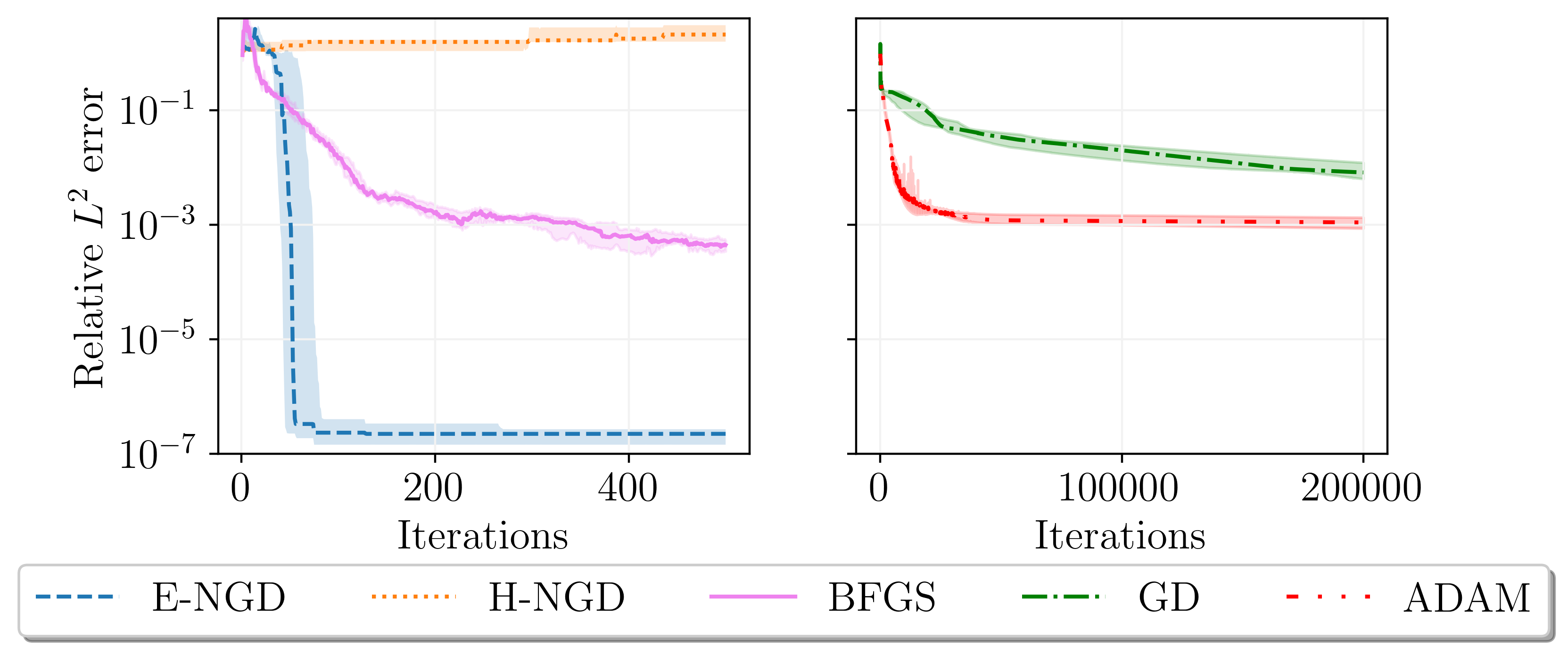
Figure 1: Median relative $L^{2}$ errors for the two dimensional Poisson equation example over 10 initializations for the five optimizers ; the shaded area denotes the region between the first and third quartile ; note that GD and Adam are run for $400$ times more iterations and GD, Adam and BFGS are given significantly more computation time than NGD, see Table 2.

	Median	Minimum	Maximum
GD	$8.2\cdot 10^{-3}$	$2.6\cdot 10^{-3}$	$1.5\cdot 10^{-2}$
Adam	$1.1\cdot 10^{-3}$	$6.9\cdot 10^{-4}$	$1.3\cdot 10^{-3}$
H-NGD	$1.2$	$4.0$	$2.1$
E-NGD	$\mathbf{2.4\cdot 10^{-7}}$	$\mathbf{1.0\cdot 10^{-7}}$	$\mathbf{4.1\cdot 10^{-7}}$
BFGS	$4.4\cdot 10^{-4}$	$1.2\cdot 10^{-4}$	$9.6\cdot 10^{-4}$

Table 1: Median, minimum and maximum of the relative $L^{2}$ errors for the Poisson equation example achieved by different optimizers over $10$ initializations. Here, energy and Hilbert NG descent and BFGS are run for $500$ and the other methods for $2\cdot 10^{5}$ iterations.

	Time per Iteration	Full Optimization Time
GD	$\mathbf{1.8\cdot 10^{-2}}\textbf{ s}$	$1\textrm{h}$
Adam	$3.7\cdot 10^{-2}\textrm{s}$	$1\text{h }6\textrm{min}$
H-NGD	$8.9\cdot 10^{-2}\textrm{s}$	$44.5\textrm{s}$
E-NGD	$8.6\cdot 10^{-2}\textrm{s}$	$\mathbf{43}\textbf{s}$
BFGS	$1.8\textrm{s}$	$15\textrm{min}$

Table 2: Computational times for the optimizers for the two dimensional Poisson example. For the time per iteration we averaged over 100 iterations. The full optimization time is calculated as the product of total iteration count and iteration time. The experiments were conducted on a single NVIDIA RTX 3080 Laptop GPU.

As reported in Table 1 and Figure 1, we observe that the energy NG updates require relatively few iterations to produce a highly accurate approximate solution of the Poisson equation. Note that the Hilbert NG descent did not converge at all, stressing the importance of employing the geometric information of the Hessian of the function space objective, as is done in energy NG descent.

The first order optimizers we consider, i.e., Adam and vanilla gradient descent reliably decrease the relative errors, but fail to achieve an accuracy higher than $6.9\cdot 10^{-4}$ even though we allow for a much higher number of iterations. The quasi-Newton method BFGS (Nocedal & Wright, 1999) achieves higher accuracy than the first order methods, however the energy natural gradient method is still roughly two orders of magnitude more accurate, compare to Table 1.

With our current implementation and the network sizes we consider, one natural gradient update is only twice to three times as costly as one iteration of the Adam algorithm, compare also to Table 2. Training a PINN model with optimizers such as Adam easily requires $100$ times the amount of iterations – without being able to produce highly accurate solutions – of what we found necessary for natural gradient training, rendering the proposed approach both faster and more accurate. Note that one optimization using the natural gradient method takes less than a minute, whereas the optimization time using the Adam optimizer takes above two hours, this is an improvement by two orders of magnitude.

To illustrate the difference between the energy natural gradient $\nabla^{E}L(\theta)$, the standard gradient $\nabla L(\theta)$ and the error $u_{\theta}-u^{*}$, we plot the effective update directions $DP(\theta)\nabla L(\theta)$ and $DP(\theta)\nabla^{E}L(\theta)$ in function space at initialization, see Figure 2. Clearly, the energy natural gradient update direction matches the error much better than the vanilla parameter gradient.

Figure 2: Shown are the error $u_{\theta}-u^{*}$ and the push forwards of the energy NG and vanilla gradient; all functions normed to lie in $[-1,1]$ to allow for a visual comparison.

4.2 An Example in Higher Dimensions

As an example in higher dimensions we consider again the Poisson equation in five spatial dimensions

$$-\Delta u =f\quad\quad\ \ \ \quad\quad\quad\text{in }[0,1]^{5},$$

$$u(x) =\sum_{k=1}^{5}\sin(\pi x_{k})\quad\ \text{on }\partial[0,1]^{5}.$$

We use the manufactured solution

$$u^{\ast}\colon\mathbb{R}^{5}\to\mathbb{R},\quad x\mapsto\sum_{k=1}^{5}\sin(\pi x_{k})$$

hence $f=\pi^{2}u^{\ast}$. For a given set of interior and boundary collocation points $(x_{1}^{i},\dots,x_{5}^{i})_{i=1,\dots,N_{\Omega}}\subseteq[0,1]^{5}$ and $(x^{b,i}_{1},\dots,x^{b,i}_{5})_{i=1,\dots,N_{\partial\Omega}}\subseteq\partial[0,1]^{5}$ we define the loss function and energy inner product exactly as in equation (14) and (15). In this example we demonstrate batched training by repeatedly drawing $N_{\Omega}=3000$ random interior and $N_{\partial\Omega}=500$ boundary collocation points in every iteration of the training process. We use a shallow neural network with input dimension 5 and 64 hidden neurons and hyperbolic tangent activation.

As presented in Figure 3, the energy natural gradient method produces highly accurate solutions in relatively short time. The convergence behavior of Adam and vanilla gradient descent again display a quickly saturating behavior and neither is able to produce competitively accurate solutions. In this example the quasi-Newton method BFGS was not able to produce more accurate solutions than the Adam optimizer. Again, E-NGD is not only the most accurate optimizer by two orders of magnitude but it achieves this accuracy while being given one order of magnitude less time.

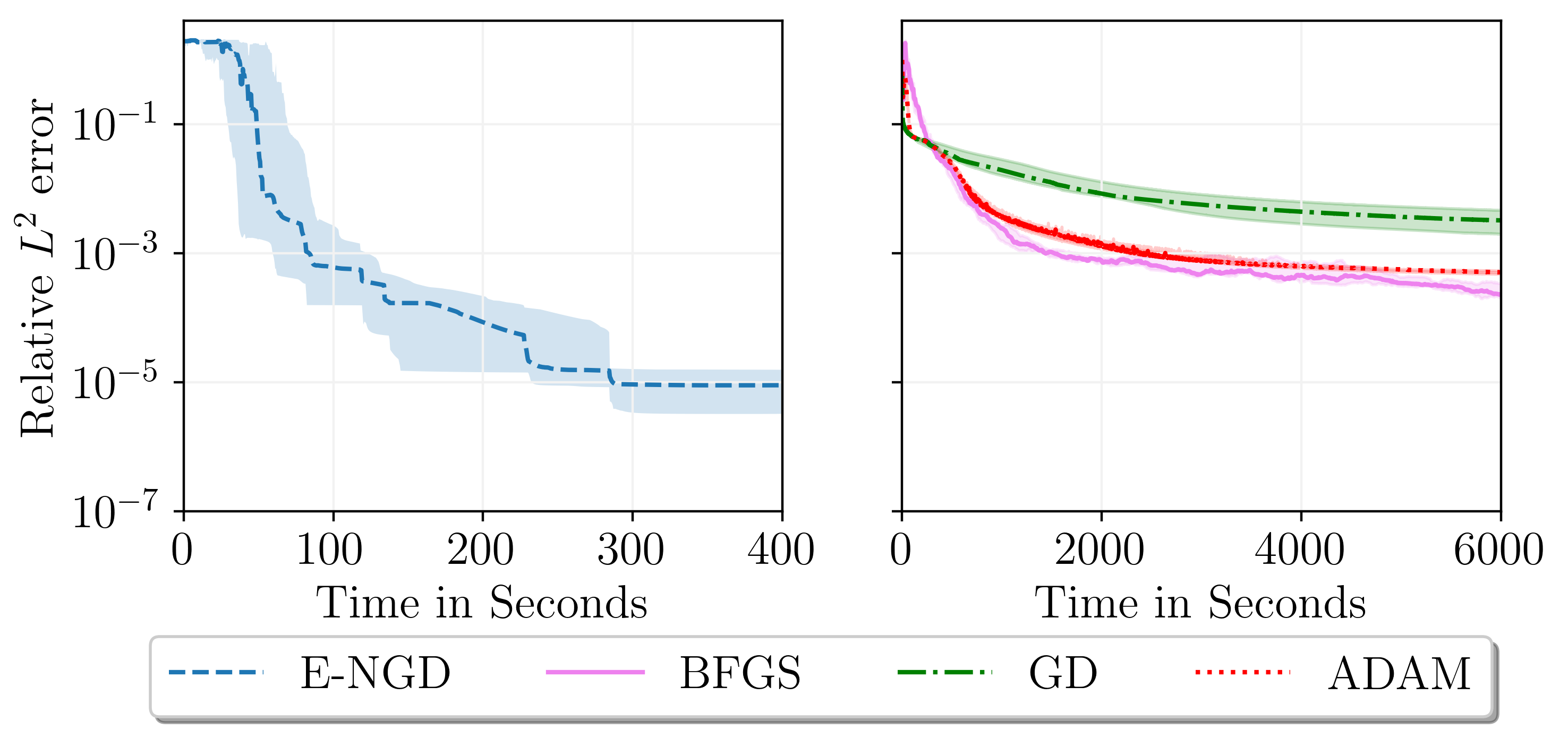
Figure 3: Median relative $L^{2}$ errors over computation time in seconds for the Poisson equation in five dimensions over 10 initializations for the optimizers: energy NG descent, vanilla gradient descent and Adam; the shaded area denotes the region between the first and third quartile. Note the different scaling of the time axis for the two plots.

4.3 Heat Equation

Let us consider the one-dimensional heat equation

$$\partial_{t}u(t,x) =\frac{1}{4}\partial_{x}^{2}u(t,x)\quad\text{for }(t,x)\in[0,1]^{2}$$

$$u(0,x) =\sin(\pi x)\qquad\;\,\text{for }x\in[0,1]$$

$$u(t,x) =0\qquad\qquad\quad\text{for }(t,x)\in[0,1]\times\{0,1\}.$$

The solution is given by

$$u^{*}(t,x)=\exp\left(-\frac{\pi^{2}t}{4}\right)\sin(\pi x)$$

and the PINN loss is

$$L(\theta) =\frac{1}{N_{\Omega_{T}}}\sum_{i=1}^{N_{\Omega_{T}}}\left(\partial_{t}u_{\theta}(t_{i},x_{i})-\frac{1}{4}\partial_{x}^{2}u_{\theta}(t_{i},x_{i})\right)^{2}$$

$$\quad+\frac{1}{N_{\text{in}}}\sum_{i=1}^{N_{\Omega}}\left(u_{\theta}(0,x_{i}^{\text{in}})-\sin(\pi x_{i}^{\text{in}})\right)^{2}$$

$$\quad+\frac{1}{N_{\partial\Omega}}\sum_{i=1}^{N_{\partial\Omega}}u_{\theta}(t^{b}_{i},x^{b}_{i})^{2},$$

where $\{(t_{i},x_{i})\}_{i=1,\dots,N_{\Omega_{T}}}$ denote collocation points in the interior of the space-time cylinder, $\{(t_{i}^{b},x_{i}^{b})\}_{i=1,\dots,N_{\partial\Omega}}$ denote collocation points on the spatial boundary and $\{(x_{i}^{\text{in}})\}_{i=1,\dots,N_{\text{in}}}$ denote collocation points for the initial condition. The energy inner product is defined on the space

$$a\colon\left(H^{1}(I,L^{2}(\Omega))\cap L^{2}(I,H^{2}(\Omega))\right)^{2}\to\mathbb{R}$$

and given by

$$a(u,v) =\int_{0}^{1}\int_{\Omega}\left(\partial_{t}u-\frac{1}{4}\partial_{x}^{2}u\right)\left(\partial_{t}v-\frac{1}{4}\partial_{x}^{2}v\right)\,\mathrm{d}x\mathrm{d}t$$

$$\quad+\int_{\Omega}u(0,x)v(0,x)\,\mathrm{d}x+\int_{I\times\partial\Omega}uv\,\mathrm{d}s\mathrm{d}t.$$

In our implementation, the inner product is discretized by the same quadrature points as in the definition of the loss function. The network architecture and the training process are identical to the previous example of the Poisson problem and we run the two NG methods for $2\cdot 10^{3}$ iterations.

Also in this example, the energy natural gradient approach shows its high accuracy and efficiency. We refer to Table 3 for the relative $L^{2}$ errors after training, Figure 4 for a visualization of the training process, Table 4 for run-times and Figure 5 for a visual comparison of the different gradients.

	Median	Minimum	Maximum
GD	$1.6\cdot 10^{-2}$	$5.0\cdot 10^{-3}$	$4.2\cdot 10^{-2}$
Adam	$1.0\cdot 10^{-3}$	$6.4\cdot 10^{-4}$	$1.4\cdot 10^{-3}$
H-NGD	$4\cdot 10^{-1}$	$3\cdot 10^{-1}$	$5\cdot 10^{-1}$
E-NGD	$\mathbf{6.3\cdot 10^{-6}}$	$\mathbf{2.3\cdot 10^{-6}}$	$5.6\cdot 10^{-1}$
BFGS	$1.4\cdot 10^{-4}$	$7.6\cdot 10^{-5}$	$\mathbf{3.3\cdot 10^{-4}}$

Table 3: Median, minimum and maximum of the relative $L^{2}$ errors for the heat equation achieved by different optimizers over $10$ different initializations. Here, H-NGD and E-NGD is run for $2\cdot 10^{3}$ and the other methods for $2\cdot 10^{5}$ iterations.

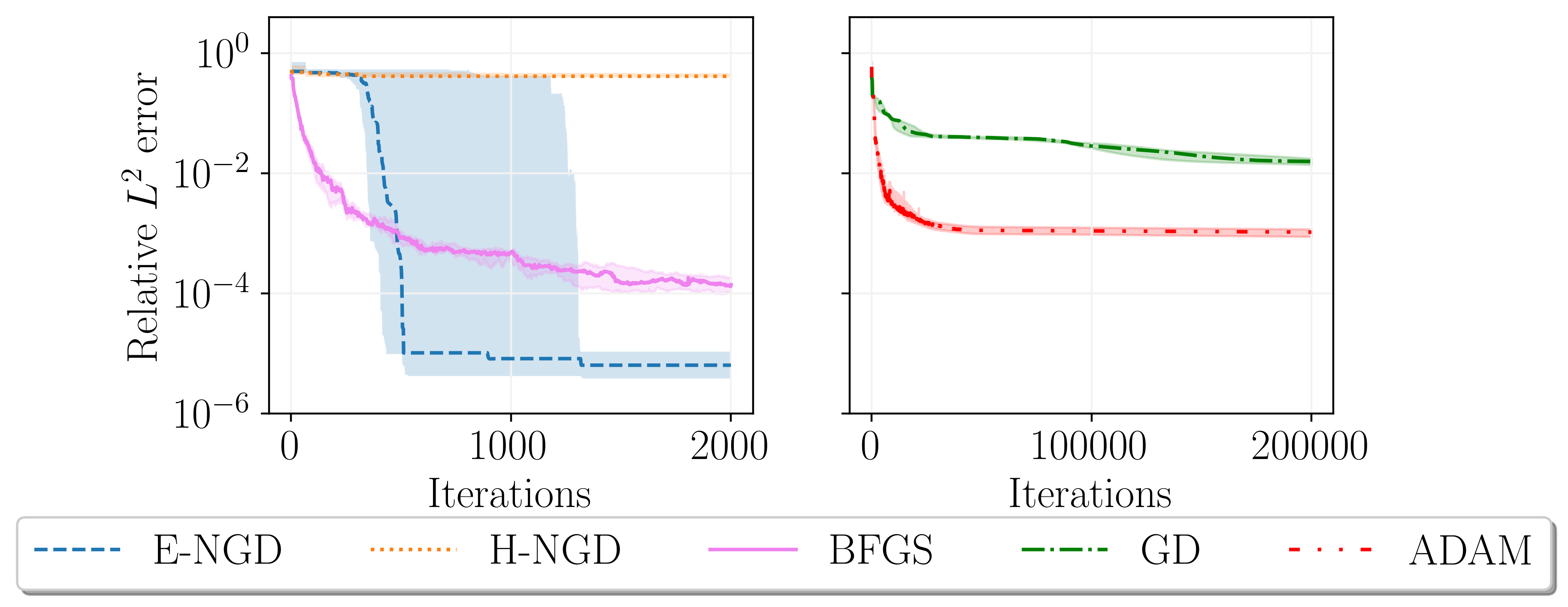
Figure 4: Relative $L^{2}$ errors for the heat equation example throughout the training process for the five optimizers. The shaded area displays the region between the first and third quartile of 10 runs for different initializations. Note that GD and Adam are run for 100 times more iterations and GD, Adam and BFGS are given significantly more computation time than NGD, see Table 4.

	Time Iteration	Time Full Optimization
GD	$\mathbf{2.2\cdot 10^{-2}}\textbf{s}$	$1\textrm{h }12\textrm{min}$
Adam	$3.8\cdot 10^{-2}\textrm{s}$	$2\textrm{h }6\textrm{min}$
E-NGD	$8.3\cdot 10^{-2}\textrm{s}$	$\mathbf{2}\textbf{min }\mathbf{48}\textbf{s}$
BFGS	$4.3\textrm{s}$	$35\textrm{min }48\textrm{s}$

Table 4: Computational time for the optimizers for the heat equation. For the time per iteration we averaged over 100 iterations. The full optimization time is calculated as the product of total iteration count and averaged iteration time. The experiments were conducted on a single NVIDIA RTX 3080 Laptop GPU.

Figure 5: The first image shows $u_{\theta}-u^{*}$, the second image is the computed natural gradient and the last image is the pushforward of the standard parameter gradient. All gradients are pointwise normed to $[-1,1]$ to allow visual comparison.

Note again the saturation of the conventional optimizers above $10^{-3}$ relative $L^{2}$ error although they are given one order of magnitude more computation time. Similar to the Poisson equation, the Hilbert NG descent is not an efficient optimization algorithm for the problem at hand which stresses again the importance of the Hessian information.

Note also, that while E-NG is highly efficient for most initializations we observed that sometimes a failure to train can occur, compare to Table 3. We did also note that conducting a pre-training, for instance with GD or Adam was in most cases able to circumvent this issue.

4.4 A Nonlinear Example with the Deep Ritz Method

We test the energy natural gradient method for a nonlinear problem utilizing the deep Ritz formulation. Consider the one-dimensional variational problem of finding the minimizer of the energy

$$E(u)\coloneqq\frac{1}{2}\int_{\Omega}|u^{\prime}|^{2}\mathrm{d}x+\frac{1}{4}\int_{\Omega}u^{4}\mathrm{d}x-\int_{\Omega}fu\,\mathrm{d}x$$ (16)

with $\Omega=[-1,1]$, $f(x)=\pi^{2}\cos(\pi x)+\cos^{3}(\pi x)$. The associated Euler Lagrange equations yield the nonlinear PDE

$$\begin{split}-u^{\prime\prime}+u^{3}&=f\quad\text{in }\Omega\\ \partial_{n}u&=0\quad\text{on }\partial\Omega\end{split}$$ (17)

and hence the minimizer is given by $u^{\ast}(x)=\cos(\pi x)$ . Since the energy is not quadratic, the energy inner product depends on $u\in H^{1}(\Omega)$ and is given by

$$D^{2}E(u)(v,w)=\int_{\Omega}v^{\prime}w^{\prime}\,\mathrm{d}x+3\int_{\Omega}u^{2}vw\,\mathrm{d}x.$$

To discretize the energy and the inner product we use trapezoidal integration with $2\cdot 10^{4}$ equi-spaced quadrature points. We use a shallow neural network of width of 32 neurons and a hyperbolic tangent as an activation function.

Once more, we observe that the energy NG updates efficiently lead to a very accurate approximation of the solution, see Figure 6 for a visualization of the training process and Table 5 for the obtained relative $L^{2}$ errors. The computation times for the individual methods are reported in Table 6.

	Median	Minimum	Maximum
GD	$2.2\cdot 10^{-4}$	$1.2\cdot 10^{-4}$	$2.6\cdot 10^{-4}$
Adam	$5.3\cdot 10^{-5}$	$2.4\cdot 10^{-5}$	$1.1\cdot 10^{-4}$
H-NGD	$\mathbf{1.0\cdot 10^{-8}}$	$6.3\cdot 10^{-9}$	$1.0$
E-NGD	$1.3\cdot 10^{-8}$	$\mathbf{6.0\cdot 10^{-9}}$	$1.0$
BFGS	$1.2\cdot 10^{-5}$	$4.7\cdot 10^{-6}$	$\mathbf{2.2\cdot 10^{-5}}$

Table 5: Median, minimum and maximum of the relative $L^{2}$ errors for the nonlinear problem achieved by different optimizers over $10$ different initializations. Here, H-NGD, E-NGD and BFGS is run for $500$ and the other methods for $2\cdot 10^{5}$ iterations.

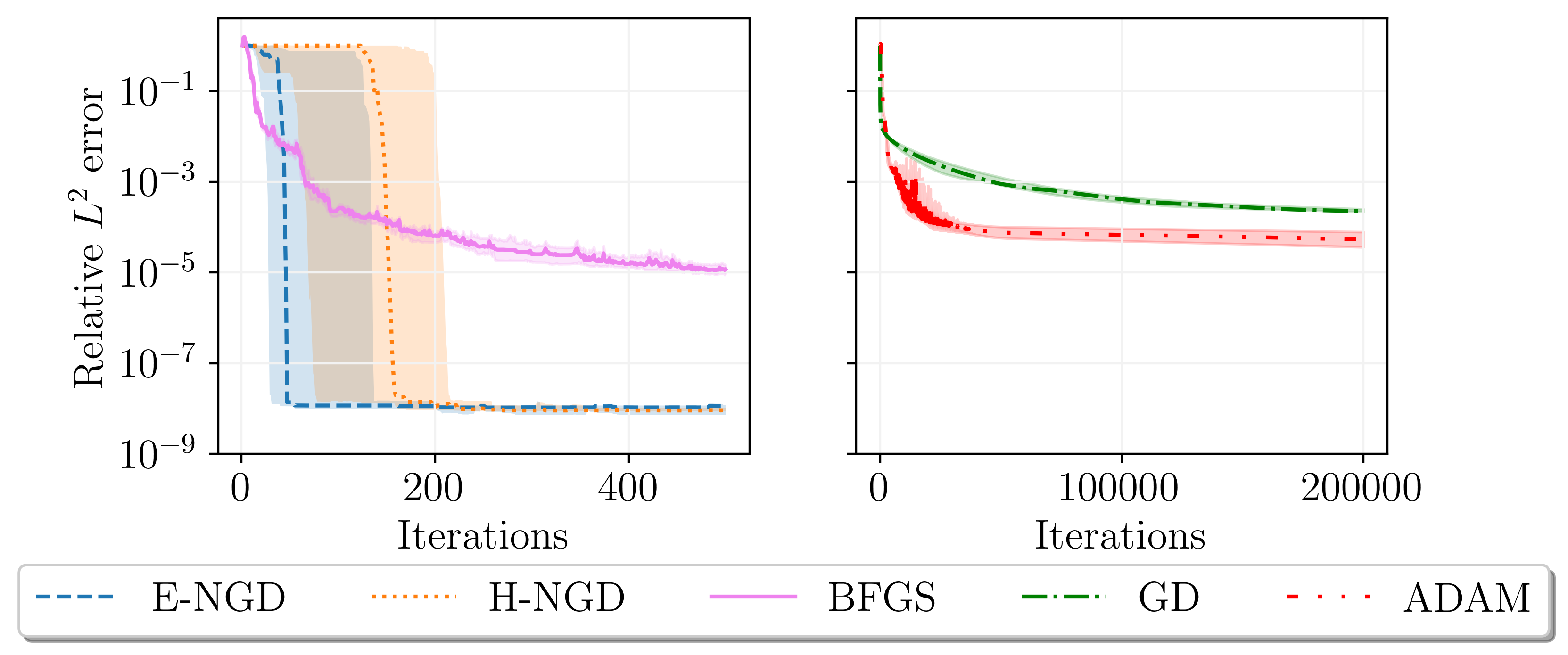
Figure 6: Relative $L^{2}$ errors for the nonlinear example throughout the training process for the five optimizers. The shaded area displays the region between the first and third quartile of 10 runs for different initializations. Note that GD and Adam are run for $400$ times more iterations and GD, Adam and BFGS are given significantly more computation time than NGD, see Table 10.

	Time per Iteration	Full Optimization Time
GD	$\mathbf{3.7\cdot 10^{-2}}\textbf{ s}$	$2\textrm{h }3\textrm{min}$
Adam	$5.8\cdot 10^{-2}\textrm{s}$	$3\text{h }13\textrm{min}$
H-NGD	$8.3\cdot 10^{-2}\textrm{s}$	$\mathbf{42}\textbf{s}$
E-NGD	$8.6\cdot 10^{-2}\textrm{s}$	$43\textrm{s}$
BFGS	$7.2\textrm{s}$	$1\text{h }$

Table 6: Computational time for the optimizers for the nonlinear example. For the time per iteration we averaged over 100 iterations. The full optimization time is calculated as the product of total iteration count and averaged iteration time. The experiments were conducted on a single NVIDIA RTX 3080 Laptop GPU.

In this example, the Hilbert NG descent is similarly efficient. Note that the energy inner product and the Hilbert space inner product are very similar in this case. Again, Adam and standard gradient descent saturate early with much higher errors than the natural gradient methods. We observe that obtaining high accuracy with the Deep Ritz method requires a highly accurate integration, which is why we used a comparatively fine grid and trapezoidal integration.

5 Conclusion

We propose to train physics informed neural networks with energy natural gradients, which correspond to the well-known concept of natural gradients combined with the geometric information of the Hessian in function space. We show that the energy natural gradient update direction corresponds to the Newton direction in function space, modulo an orthogonal projection onto the tangent space of the model. We demonstrate experimentally that this optimization achieves highly accurate PINN solutions, well beyond the the accuracy that can be obtained with standard optimizers even if these methods are allowed several order of magnitude more computation time. The proposed method is compatible with arbitrary discretizations of the integrals appearing in the objective and the gram matrix as with arbitrary network architectures. Important future directions include the development of efficient implementations of energy natural gradients for large scale problems and the development of specialized initialization schemes.

Appendix A Proofs Regarding NGs in Function Space

We follow an analogue approach to (van Oostrum et al., 2022), which considers finite dimensional spaces.

Lemma 3.

Let $X$ be a vector space with a scalar product $\langle\cdot,\cdot\rangle\colon X\times X\to\mathbb{R}$ and consider a linear map $A\colon\mathbb{R}^{p}\to X$ for some $p\in\mathbb{N}$. Let $G\in\mathbb{R}^{p\times p}$ be given by $G_{ij}\coloneqq\langle Ae_{i},Ae_{j}\rangle$ and consider the adjoint operator $A^{\ast}\colon X\to\mathbb{R}^{p}$ given by

$$A^{\ast}y\coloneqq\sum_{i=1}^{p}\langle y,Ae_{i}\rangle e_{i}.$$ (18)

Then it holds that

$$AG^{+}A^{\ast}x=\Pi_{R(A)}(x),$$ (19)

where $\Pi_{R(A)}(x)$ denotes the projection of $x$ onto the range $R(A)=\{Av:v\in\mathbb{R}^{p}\}$ of $A$, which is the unique element satisfying

$$\langle\Pi_{R(A)}(x),z\rangle=\langle x,z\rangle\quad\text{for all }z\in R(A).$$ (20)

Proof.

It is elementary to check that the adjoint satisfies $\langle A^{\ast}x,v\rangle=\langle x,Av\rangle$. Picking some orthonormal basis $(b_{i})_{i=1,\dots,d}$ of $R(A)$, the orthogonal projection of $x\in X$ to $R(A)$ exists and is given by $\sum_{i}\langle x,b_{i}\rangle b_{i}$. Without loss of generality we can assume $x\in R(A)$ and otherwise replace $x$ by its projection onto $R(A)$ since $A^{\ast}$ vanishes on $R(A)^{\perp}$.

Let us use the notation $v_{i}\coloneqq Ae_{i}$. Note that clearly $AG^{+}A^{\ast}x\in R(A)$. Hence, it remains to show that $\langle AG^{+}A^{\ast}x,v_{i}\rangle=\langle x,v_{i}\rangle$ for all $i=1,\dots,p$. It holds that $A^{\ast}v_{i}=\sum_{j}\langle Ae_{i},Ae_{j}\rangle e_{j}=Ge_{i}$ and we can express $x=\sum_{i}a_{i}v_{i}$. Using the symmetry of $G$ we can compute

$$\begin{split}\langle AG^{+}A^{\ast}x,v_{i}\rangle&=\langle G^{+}A^{\ast}x,A^{\ast}v_{i}\rangle\\ &=\sum_{j}a_{j}\langle G^{+}A^{\ast}v_{j},Ge_{i}\rangle\\ &=\sum_{j}a_{j}\langle GG^{+}Ge_{j},e_{i}\rangle\\ &=\sum_{j}a_{j}\langle Ge_{j},e_{i}\rangle\\ &=\sum_{j}a_{j}\langle A^{\ast}v_{j},e_{i}\rangle\\ &=\sum_{j}a_{j}\langle v_{j},Ae_{i}\rangle\\ &=\langle x,v_{i}\rangle,\end{split}$$ (21)

which completes the proof. ∎

Theorem 4 (NG for Hilbert Manifolds).

Let $(\mathcal{M},g)$ be a Riemannian Hilbert manifold with model space $X$, where for any $x\in\mathcal{M}$ the Riemannian metric $g_{x}$ defines a scalar product on the tangent space $T_{x}\mathcal{M}\cong X$ rendering $T_{x}\mathcal{M}$ complete. Assume a differentiable objective function $E\colon\mathcal{M}\to\mathbb{R}$ and a differentiable parametrization $P\colon\mathbb{R}^{p}\to\mathcal{M}$ and define the Gram matrix in the usual way $G(\theta)_{ij}\coloneqq g_{P(\theta)}(\partial_{\theta_{i}}P(\theta),\partial_{\theta_{j}}P(\theta))$ and consider the objective function $L\colon\mathbb{R}^{p}\to\mathbb{R},\theta\mapsto E(u_{\theta})$.Then it holds that

$$DP_{\theta}G(\theta)^{+}\nabla L(\theta)=\Pi_{T_{\theta}P(\mathbb{R}^{p})}\nabla E(P(\theta)).$$ (22)

Proof.

This follows directly from Lemma 3 by setting $X\coloneqq T_{P(\theta)}\mathcal{M}$ and $A=DP_{\theta}$, where by the gradient chain rule it holds that $\nabla L(\theta)=DP(\theta)^{\ast}\nabla E(u_{\theta})$. ∎

See 2

Proof.

The case of strongly convex energy $E$ is a falls into the setting of Theorem 4 by defining the Riemannian metric via $g_{u}\coloneqq DE^{2}(u)$. It remains to show that the Riemannian gradient with respect to the metric induced by the second derivative $D^{2}E$ is given by $D^{2}E(u)^{-1}\nabla E(u)$. This follows from

$$\begin{split}D^{2}E(u)(D^{2}E(u)^{-1}\nabla E(u),v)=\langle\nabla E(u),v\rangle=DE(u)v.\end{split}$$ (23)

Consider now the case of a symmetric quadratic function $E$ with positiv definite second derivative $D^{2}E$ and assume that $E$ admits a unique minimizer $u^{\ast}\in X$. Lemma 3 with $A=DP_{\theta}$ implies

$$\begin{split}DP_{\theta}G(\theta)^{+}DP_{\theta}^{\ast,a}(u-u^{\ast})=\Pi_{T_{\theta}\mathcal{F}_{\Theta}}(u-u^{\ast}),\end{split}$$ (24)

where $DP_{\theta}^{\ast,a}$ denotes the adjoint of $DP_{\theta}$ with respect to the inner product $a$. Hence, it remains to show $\nabla L(\theta)=DP_{\theta}^{\ast,a}(u-u^{\ast})$. Note that $E(u)=\frac{1}{2}a(u-u^{\ast},u-u^{\ast})+c$ for a suitable constant $c\in\mathbb{R}$. This follows from the computation

$$\begin{split}\langle DP_{\theta}^{\ast,a}(u-u^{\ast}),e_{i}\rangle_{\mathbb{R}^{p}}&=a(u_{\theta}-u^{\ast},DP_{\theta}e_{i})\\ &=a(u_{\theta}-u^{\ast},\partial_{\theta_{i}}u_{\theta})\\ &=DE(u_{\theta})\partial_{\theta_{i}}u_{\theta}\\ &=\partial_{\theta_{i}}L(\theta),\end{split}$$ (25)

where we used the chain rule in the last step. ∎

Appendix B Additional Resources for the Experiments

B.1 Relative $H^{1}$ Errors

For completeness sake, we report the $H^{1}$ errors of the three experiments in the main part of the manuscript.

Relative $H^{1}$ errors after training

First, we present the relative $H^{1}$ errors obtained at the end of training in Tables 7-9.

	Median	Minimum	Maximum
GD	$9.3\cdot 10^{-2}$	$2.6\cdot 10^{-2}$	$1.4\cdot 10^{-1}$
Adam	$1.5\cdot 10^{-2}$	$9.1\cdot 10^{-3}$	$2.5\cdot 10^{-2}$
H-NGD	$7.0$	$5.2$	$12.4$
E-NGD	$\mathbf{4.9\cdot 10^{-6}}$	$\mathbf{2.6\cdot 10^{-6}}$	$\mathbf{1.0\cdot 10^{-5}}$
BFGS	$6.0\cdot 10^{-3}$	$1.3\cdot 10^{-3}$	$1.7\cdot 10^{-2}$

Table 7: Median, minimum and maximum of the relative $H^{1}$ errors for the Poisson equation achieved by different optimizers over $10$ different initializations. Here, H-NGD, E-NGD and BFGS is run for $500$ and the other methods for $2\cdot 10^{5}$ iterations.

	Median	Minimum	Maximum
GD	$1.8\cdot 10^{-1}$	$7.4\cdot 10^{-2}$	$4.5\cdot 10^{-1}$
Adam	$1.7\cdot 10^{-2}$	$1.2\cdot 10^{-2}$	$2.5\cdot 10^{-2}$
H-NGD	$2.9$	$2.6$	$3.0$
E-NGD	$\mathbf{1.8\cdot 10^{-4}}$	$\mathbf{8.2\cdot 10^{-5}}$	$3.1$
BFGS	$2.8\cdot 10^{-3}$	$1.3\cdot 10^{-3}$	$\mathbf{6.7\cdot 10^{-3}}$

Table 8: Median, minimum and maximum of the relative $H^{1}$ errors for the heat equation achieved by different optimizers over $10$ different initializations. Here, H-NGD, E-NGD and BFGS is run for $2000$ and the other methods for $2\cdot 10^{5}$ iterations.

	Median	Minimum	Maximum
GD	$6.1\cdot 10^{-3}$	$3.6\cdot 10^{-3}$	$9.1\cdot 10^{-3}$
Adam	$1.8\cdot 10^{-3}$	$7.5\cdot 10^{-4}$	$3.7\cdot 10^{-3}$
H-NGD	$\mathbf{8.1\cdot 10^{-7}}$	$\mathbf{5.5\cdot 10^{-7}}$	$8.3$
E-NGD	$9.3\cdot 10^{-7}$	$6.0\cdot 10^{-7}$	$8.3$
BFGS	$2.4\cdot 10^{-4}$	$7.9\cdot 10^{-5}$	$\mathbf{4.1\cdot 10^{-4}}$

Table 9: Median, minimum and maximum of the relative $H^{1}$ errors for the nonlinear equation achieved by different optimizers over $10$ different initializations. Here, H-NGD, E-NGD and BFGS is run for $500$ and the other methods for $2\cdot 10^{5}$ iterations. At the moment only a single initialization of BFGS is run.

Relative $H^{1}$ Errors During Training

Furthermore, we provide also the visualizations of the training processes of the experiments of the main section when the error is measured in $H^{1}$ norm.

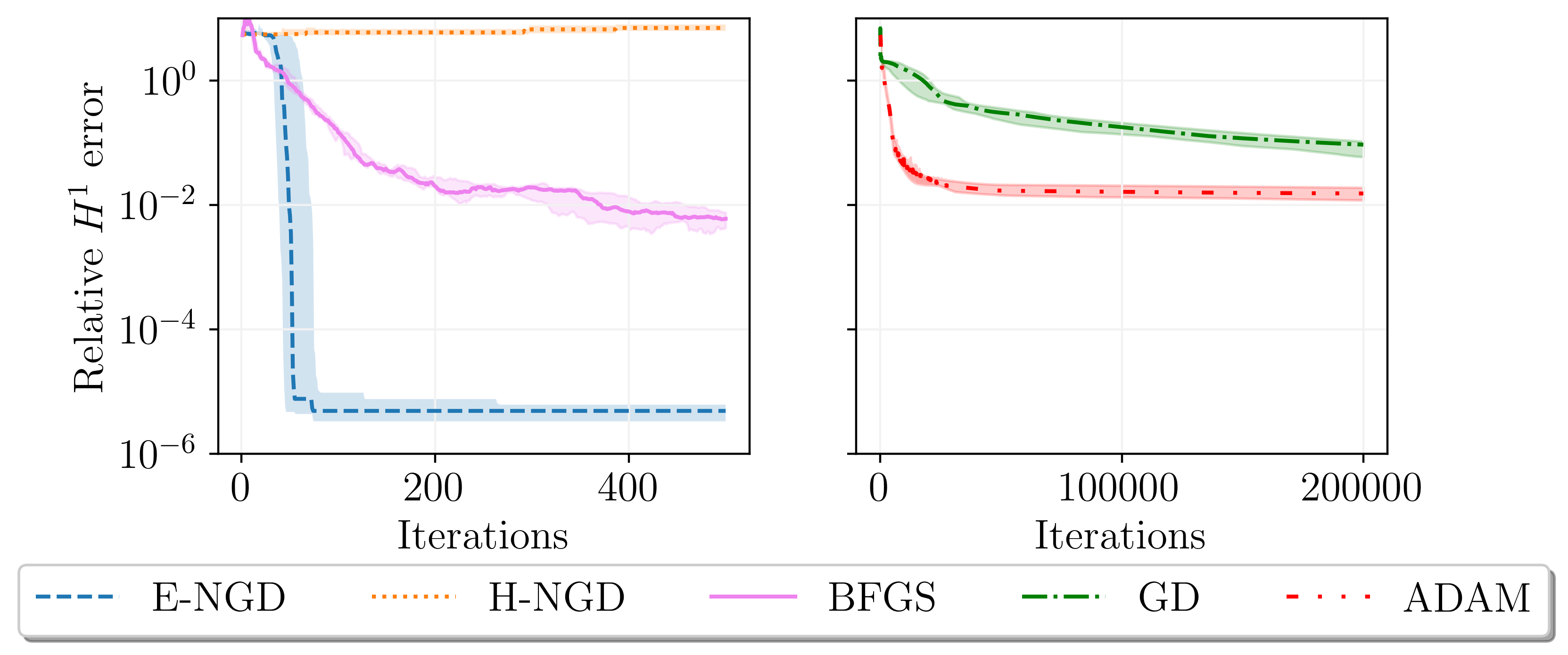
Figure 7: The plot shows the median of the relative $H^{1}$ errors for the Poisson equation throughout the training process for the five optimizers: energy natural gradient descent, Hilbert natural gradient descent, BFGS, vanilla gradient descent and Adam. The shaded area displays the region between the first and third quartile of 10 runs for different initializations of the network’s parameters. Note that GD and Adam are run for 400 times more iterations.

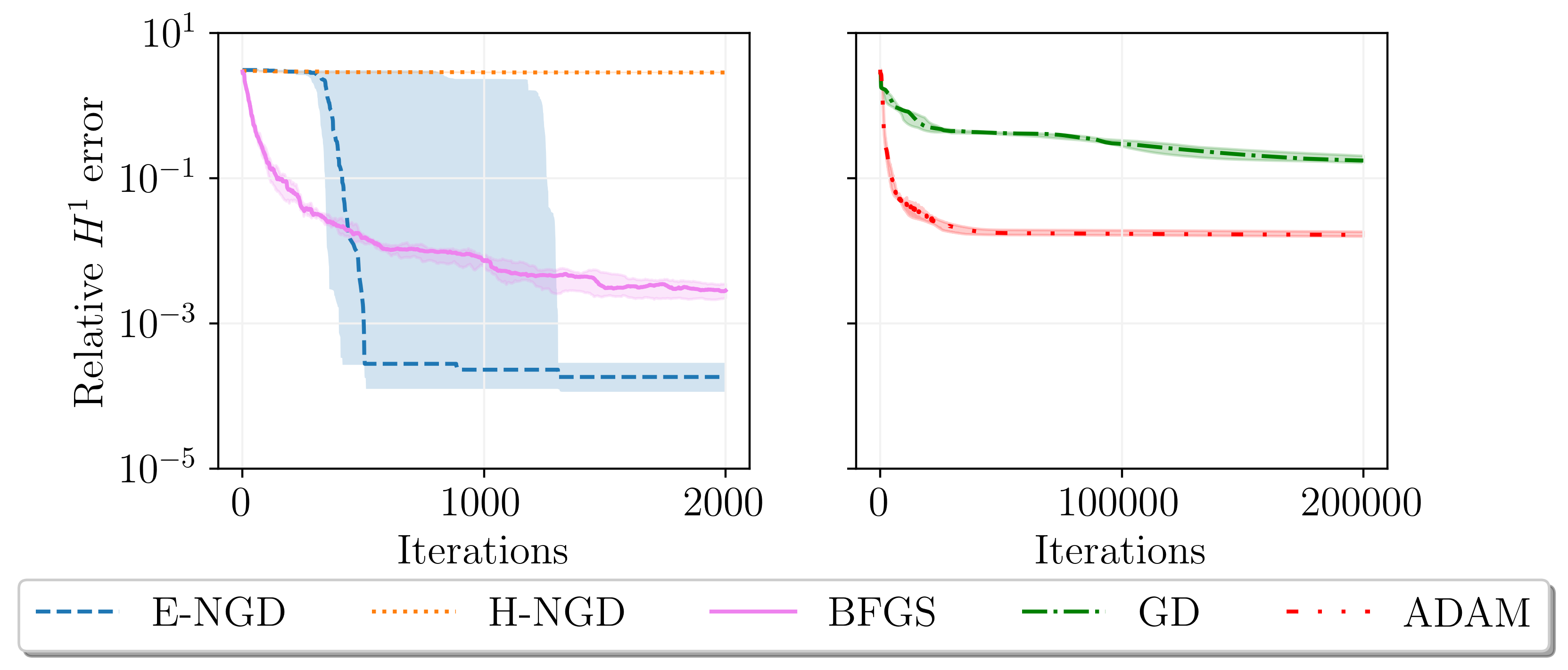
Figure 8: The plot shows the median of the relative $H^{1}$ errors for the heat equation throughout the training process for the five optimizers: energy natural gradient descent, Hilbert natural gradient descent, BFGS, vanilla gradient descent and Adam. The shaded area displays the region between the first and third quartile of 10 runs for different initializations of the network’s parameters. Note that GD and Adam are run for 100 times more iterations.

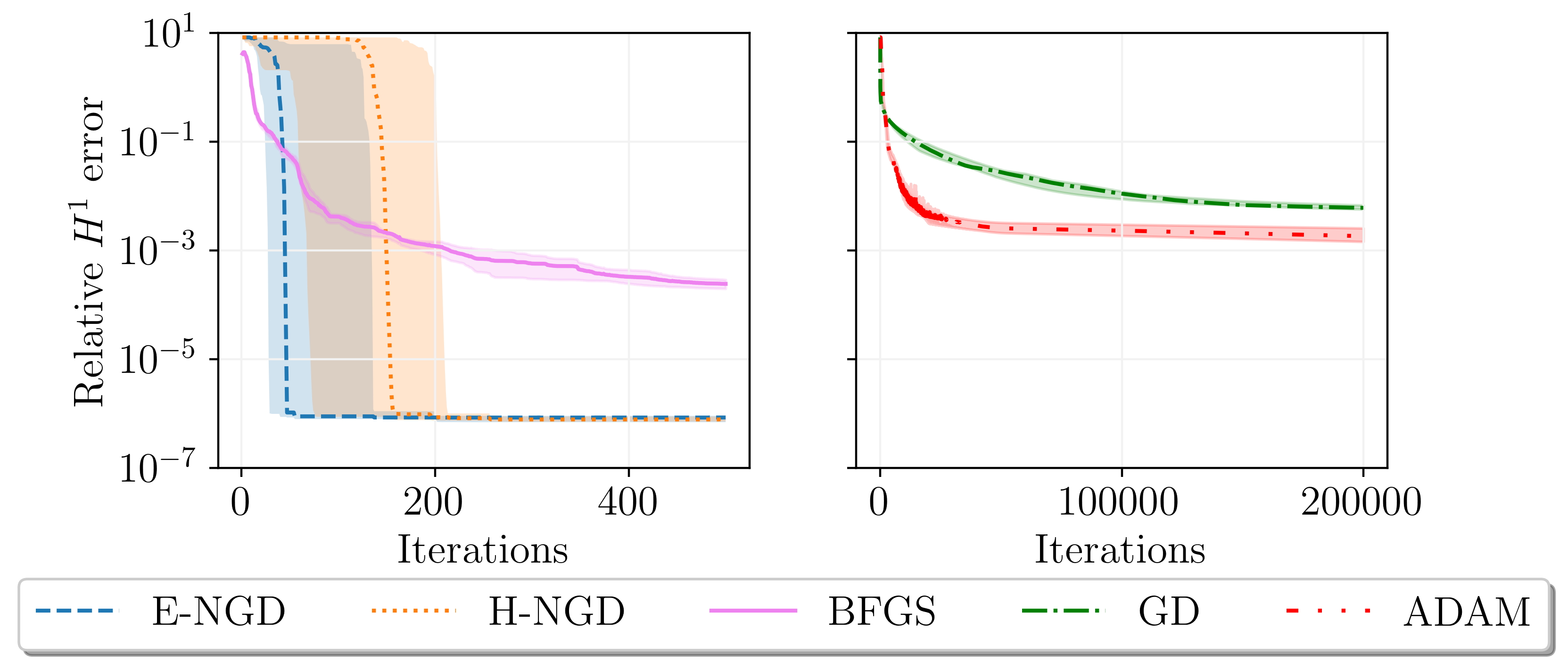
Figure 9: The plot shows the median of the relative $H^{1}$ errors for the nonlinear example throughout the training process for the five optimizers: energy natural gradient descent, Hilbert natural gradient descent, BFGS, vanilla gradient descent and Adam. The shaded area displays the region between the first and third quartile of 10 runs for different initializations of the network’s parameters. Note that GD and Adam are run for 400 times more iterations.

B.2 Training a Deep Network

To demonstrate the capability of the energy natural gradient method to be applied to larger and deeper networks, we use the two dimensional Poisson example from section 4.1 and employ a network with three hidden layers of width 50, which corresponds to roughly 5k trainable weights. We train the network for only 100 iterations. Apart from this we keep all other settings unchanged. We report the results in Table 10.

	Median $L^{2}$ Error	Time Iter	Time Full
E-NGD	$2.5\cdot 10^{-6}$	$1.1\textrm{min}$	$1.8\textrm{h}$

Table 10: Results for the ENGD training of the deep network for the two dimensional Poisson equation. Reported is the median $L^{2}$ error over 10 initializations, the time for one iteration and the full optimization time.

We conclude that the energy natural gradient approach can be used for larger and deeper networks, albeit at a higher computational cost. Note however, that we could reduce the amount of iterations required to obtain convergence. The the small networks considered in the main part of the manuscript perform equally well for our tasks at hand, which explains why we did not choose deep networks.

References

- Amari (1998) Amari, S. Natural gradient works efficiently in learning. Neural computation, 10(2):251–276, 1998.
- Amari (2016) Amari, S. Information geometry and its applications, volume 194. Springer, Japan, 2016.
- Amari & Cichocki (2010) Amari, S. and Cichocki, A. Information geometry of divergence functions. Bulletin of the Polish academy of sciences. Technical sciences, 58(1):183–195, 2010.
- Bagnell & Schneider (2003) Bagnell, J. A. and Schneider, J. G. Covariant policy search. In IJCAI, pp. 1019–1024, 2003.
- Beck et al. (2020) Beck, C., Hutzenthaler, M., Jentzen, A., and Kuckuck, B. An overview on deep learning-based approximation methods for partial differential equations. arXiv preprint arXiv:2012.12348, 2020.
- Bradbury et al. (2018) Bradbury, J., Frostig, R., Hawkins, P., Johnson, M. J., Leary, C., Maclaurin, D., Necula, G., Paszke, A., VanderPlas, J., Wanderman-Milne, S., and Zhang, Q. JAX: composable transformations of Python+NumPy programs, 2018. URL http://github.com/google/jax.
- Cai et al. (2019) Cai, T., Gao, R., Hou, J., Chen, S., Wang, D., He, D., Zhang, Z., and Wang, L. Gram-gauss-newton method: Learning overparameterized neural networks for regression problems. arXiv preprint arXiv:1905.11675, 2019.
- Courte & Zeinhofer (2023) Courte, L. and Zeinhofer, M. Robin Pre-Training for the Deep Ritz Method. Northern Lights Deep Learning Conference, 2023.
- Davi & Braga-Neto (2022) Davi, C. and Braga-Neto, U. Pso-pinn: Physics-informed neural networks trained with particle swarm optimization. arXiv preprint arXiv:2202.01943, 2022.
- Daw et al. (2022) Daw, A., Bu, J., Wang, S., Perdikaris, P., and Karpatne, A. Rethinking the importance of sampling in physics-informed neural networks. arXiv preprint arXiv:2207.02338, 2022.
- Dissanayake & Phan-Thien (1994) Dissanayake, M. and Phan-Thien, N. Neural-network-based approximations for solving partial differential equations. communications in Numerical Methods in Engineering, 10(3):195–201, 1994.
- E & Yu (2018) E, W. and Yu, B. The Deep Ritz Method: A Deep Learning-Based Numerical Algorithm for Solving Variational Problems. Communications in Mathematics and Statistics, 6(1):1–12, 2018.
- E et al. (2017) E, W., Han, J., and Jentzen, A. Deep learning-based numerical methods for high-dimensional parabolic partial differential equations and backward stochastic differential equations. Communications in Mathematics and Statistics, 5(4):349–380, 2017.
- Gargiani et al. (2020) Gargiani, M., Zanelli, A., Diehl, M., and Hutter, F. On the promise of the stochastic generalized gauss-newton method for training dnns. arXiv preprint arXiv:2006.02409, 2020.
- Han et al. (2018) Han, J., Jentzen, A., and Weinan, E. Solving high-dimensional partial differential equations using deep learning. Proceedings of the National Academy of Sciences, 115(34):8505–8510, 2018.
- Hao et al. (2021) Hao, W., Jin, X., Siegel, J. W., and Xu, J. An efficient greedy training algorithm for neural networks and applications in PDEs. arXiv preprint arXiv:2107.04466, 2021.
- Kakade (2001) Kakade, S. M. A natural policy gradient. Advances in Neural Information Processing Systems, 14, 2001.
- Kovachki et al. (2021) Kovachki, N., Li, Z., Liu, B., Azizzadenesheli, K., Bhattacharya, K., Stuart, A., and Anandkumar, A. Neural operator: Learning maps between function spaces. arXiv preprint arXiv:2108.08481, 2021.
- Krishnapriyan et al. (2021) Krishnapriyan, A., Gholami, A., Zhe, S., Kirby, R., and Mahoney, M. W. Characterizing possible failure modes in physics-informed neural networks. Advances in Neural Information Processing Systems, 34:26548–26560, 2021.
- Lagaris et al. (1998) Lagaris, I. E., Likas, A., and Fotiadis, D. I. Artificial neural networks for solving ordinary and partial differential equations. IEEE transactions on neural networks, 9(5):987–1000, 1998.
- Li & Montúfar (2018) Li, W. and Montúfar, G. Natural gradient via optimal transport. Information Geometry, 1(2):181–214, 2018. URL https://doi.org/10.1007/s41884-018-0015-3.
- Li et al. (2021) Li, Z., Kovachki, N. B., Azizzadenesheli, K., liu, B., Bhattacharya, K., Stuart, A., and Anandkumar, A. Fourier neural operator for parametric partial differential equations. In International Conference on Learning Representations, 2021. URL https://openreview.net/forum?id=c8P9NQVtmnO.
- Lin et al. (2021) Lin, A. T., Li, W., Osher, S., and Montúfar, G. Wasserstein proximal of gans. In International Conference on Geometric Science of Information, pp. 524–533. Springer, 2021.
- Lu et al. (2021) Lu, L., Meng, X., Mao, Z., and Karniadakis, G. E. Deepxde: A deep learning library for solving differential equations. SIAM Review, 63(1):208–228, 2021.
- Martens (2020) Martens, J. New insights and perspectives on the natural gradient method. The Journal of Machine Learning Research, 21(1):5776–5851, 2020.
- Morimura et al. (2008) Morimura, T., Uchibe, E., Yoshimoto, J., and Doya, K. A new natural policy gradient by stationary distribution metric. In Joint European Conference on Machine Learning and Knowledge Discovery in Databases, pp. 82–97. Springer, 2008.
- Müller & Montúfar (2022) Müller, J. and Montúfar, G. Geometry and convergence of natural policy gradients. MPI MiS Preprint 31/2022, 2022. URL https://www.mis.mpg.de/publications/preprints/2022/prepr2022-31.html.
- Müller & Zeinhofer (2022a) Müller, J. and Zeinhofer, M. Error estimates for the deep ritz method with boundary penalty. In Mathematical and Scientific Machine Learning, pp. 215–230. PMLR, 2022a.
- Müller & Zeinhofer (2022b) Müller, J. and Zeinhofer, M. Notes on exact boundary values in residual minimisation. In Mathematical and Scientific Machine Learning, pp. 231–240. PMLR, 2022b.
- Nabian et al. (2021) Nabian, M. A., Gladstone, R. J., and Meidani, H. Efficient training of physics-informed neural networks via importance sampling. Computer-Aided Civil and Infrastructure Engineering, 36(8):962–977, 2021.
- Nocedal & Wright (1999) Nocedal, J. and Wright, S. J. Numerical optimization. Springer, 1999.
- Nurbekyan et al. (2022) Nurbekyan, L., Lei, W., and Yang, Y. Efficient natural gradient descent methods for large-scale optimization problems. arXiv:2202.06236, 2022.
- Pascanu & Bengio (2014) Pascanu, R. and Bengio, Y. Revisiting natural gradient for deep networks. In International Conference on Learning Representations, 2014. URL https://openreview.net/forum?id=vz8AumxkAfz5U.
- Peters et al. (2003) Peters, J., Vijayakumar, S., and Schaal, S. Reinforcement learning for humanoid robotics. In Proceedings of the third IEEE-RAS international conference on humanoid robots, pp. 1–20, 2003.
- Raissi et al. (2019) Raissi, M., Perdikaris, P., and Karniadakis, G. E. Physics-informed neural networks: A deep learning framework for solving forward and inverse problems involving nonlinear partial differential equations. Journal of Computational physics, 378:686–707, 2019.
- Ren & Goldfarb (2019) Ren, Y. and Goldfarb, D. Efficient subsampled gauss-newton and natural gradient methods for training neural networks. arXiv preprint arXiv:1906.02353, 2019.
- Ritz (1909) Ritz, W. Über eine neue Methode zur Lösung gewisser Variationsprobleme der mathematischen Physik. Journal für die reine und angewandte Mathematik (Crelles Journal), 1909(135):1–61, 1909.
- Schraudolph (2002) Schraudolph, N. N. Fast curvature matrix-vector products for second-order gradient descent. Neural computation, 14(7):1723–1738, 2002.
- Schwedes et al. (2016) Schwedes, T., Funke, S. W., and Ham, D. A. An iteration count estimate for a mesh-dependent steepest descent method based on finite elements and Riesz inner product representation. arXiv preprint arXiv:1606.08069, 2016.
- Schwedes et al. (2017) Schwedes, T., Ham, D. A., Funke, S. W., and Piggott, M. D. Mesh dependence in PDE-constrained optimisation. In Mesh Dependence in PDE-Constrained Optimisation, pp. 53–78. Springer, 2017.
- Shen et al. (2020) Shen, Z., Wang, Z., Ribeiro, A., and Hassani, H. Sinkhorn natural gradient for generative models. Advances in Neural Information Processing Systems, 33:1646–1656, 2020.
- Sirignano & Spiliopoulos (2018) Sirignano, J. and Spiliopoulos, K. DGM: A deep learning algorithm for solving partial differential equations. Journal of computational physics, 375:1339–1364, 2018.
- Thomas et al. (2016) Thomas, P., Silva, B. C., Dann, C., and Brunskill, E. Energetic natural gradient descent. In International Conference on Machine Learning, pp. 2887–2895. PMLR, 2016.
- van der Meer et al. (2022) van der Meer, R., Oosterlee, C. W., and Borovykh, A. Optimally weighted loss functions for solving pdes with neural networks. Journal of Computational and Applied Mathematics, 405:113887, 2022.
- van Oostrum et al. (2022) van Oostrum, J., Müller, J., and Ay, N. Invariance properties of the natural gradient in overparametrised systems. Information Geometry, pp. 1–17, 2022.
- Wang & Yan (2022) Wang, L. and Yan, M. Hessian informed mirror descent. Journal of Scientific Computing, 92(3):1–22, 2022.
- Wang et al. (2021) Wang, S., Teng, Y., and Perdikaris, P. Understanding and mitigating gradient flow pathologies in physics-informed neural networks. SIAM Journal on Scientific Computing, 43(5):A3055–A3081, 2021.
- Wang et al. (2022a) Wang, S., Sankaran, S., and Perdikaris, P. Respecting causality is all you need for training physics-informed neural networks. arXiv preprint arXiv:2203.07404, 2022a.
- Wang et al. (2022b) Wang, S., Yu, X., and Perdikaris, P. When and why PINNs fail to train: A neural tangent kernel perspective. Journal of Computational Physics, 449:110768, 2022b.
- Weinan et al. (2021) Weinan, E., Han, J., and Jentzen, A. Algorithms for solving high dimensional PDEs: from nonlinear monte carlo to machine learning. Nonlinearity, 35(1):278, 2021.
- Wu et al. (2023) Wu, C., Zhu, M., Tan, Q., Kartha, Y., and Lu, L. A comprehensive study of non-adaptive and residual-based adaptive sampling for physics-informed neural networks. Computer Methods in Applied Mechanics and Engineering, 403:115671, 2023.
- Zapf et al. (2022) Zapf, B., Haubner, J., Kuchta, M., Ringstad, G., Eide, P. K., and Mardal, K.-A. Investigating molecular transport in the human brain from mri with physics-informed neural networks. Scientific Reports, 12(1):1–12, 2022.
- Zeng et al. (2022) Zeng, Q., Bryngelson, S. H., and Schaefer, F. T. Competitive physics informed networks. In ICLR 2022 Workshop on Gamification and Multiagent Solutions, 2022. URL https://openreview.net/forum?id=rMz_scJ6lc.