Continuous gap contact formulation based on the screened Poisson equation

Abstract

We introduce a PDE-based node-to-element contact formulation as an alternative to classical, purely geometrical formulations. It is challenging to devise solutions to nonsmooth contact problem with continuous gap using finite element discretizations. We herein achieve this objective by constructing an approximate distance function (ADF) to the boundaries of solid objects, and in doing so, also obtain universal uniqueness of contact detection. Unilateral constraints are implemented using a mixed model combining the screened Poisson equation and a force element, which has the topology of a continuum element containing an additional incident node. An ADF is obtained by solving the screened Poisson equation with constant essential boundary conditions and a variable transformation. The ADF does not explicitly depend on the number of objects and a single solution of the partial differential equation for this field uniquely defines the contact conditions for all incident points in the mesh. Having an ADF field to any obstacle circumvents the multiple target surfaces and avoids the specific data structures present in traditional contact-impact algorithms. We also relax the interpretation of the Lagrange multipliers as contact forces, and the Courant–Beltrami function is used with a mixed formulation producing the required differentiable result. We demonstrate the advantages of the new approach in two- and three-dimensional problems that are solved using Newton iterations. Simultaneous constraints for each incident point are considered.

^aDEM - Departamento de Engenharia Mecânica
Instituto Superior Tï¿œcnico
Universidade de Lisboa
Building Mechanics II, Avenida Rovisco Pais 1, 1049-001
Lisboa, Portugal
^bIDMEC - Instituto Superior Tï¿œcnico
Avenida Rovisco Pais 1, 1049-001
Lisboa, Portugal
^cUC-Davis - University of California at Davis
Department of Civil & Environmental Engineering
One Shields Avenue
Davis, CA 95616. U.S.A
^⋆pedro.areias@tecnico.ulisboa.pt

KEYWORDS: nonsmooth contact geometries, contact algorithm, finite strains, Eikonal equation, approximate distance function, screened Poisson equation

1 Introduction

Considerable interest has recently emerged with the enforcement of essential boundary conditions [1] and contact detection algorithms [2] using approximate distance functions (ADFs). Realistic contact frameworks for finite-strain problems make use of three classes of algorithms that are often coupled (see [3]):

1. Techniques of unilateral constraint enforcement. Examples of these are direct elimination (also reduced-gradient algorithms), penalty and barrier methods, and Lagrange multiplier methods with the complementarity condition [4]. Stresses from the underlying discretization are often used to assist the normal condition with Nitsche’s method [5].

2. Frictional effects (and more generally, constitutive contact laws) and cone-complementarity forms [6, 7]. Solution paradigms are augmented Lagrangian methods for friction [8], cone-projection techniques [9] and the so-called yield-limited algorithm for friction [10].

3. Discretization methods. Of concern are distance calculations, estimation of tangent velocities and general discretization arrangements. In contemporaneous use are (see [3]) node-to-edge/face, edge/face-to-/edge/face and mortar discretizations.

In terms of contact enforcement and friction algorithms, finite displacement contact problems are typically addressed with well-established contact algorithms, often derived from solutions developed by groups working on variational inequalities and nonsmooth analysis. However, in the area of contact discretization and the related area of contact kinematics [11], there are still challenges to be addressed in terms of ensuring the complete robustness of implicit codes. One of the earliest papers on contact discretization was by Chan and Tuba [12], who considered contact with a plane and used symmetry to analyze cylinder-to-cylinder contact. Francavilla and Zienkiewicz [13] later proposed an extension to node-to-node contact in small strains, allowing for direct comparison with closed-form solutions. The extension to finite strains requires further development, and the logical development was the node-to-segment approach, as described in the work of Hallquist [14]. Although node-to-segment algorithms are known to entail many defficiencies, most of the drawbacks have been addressed. Jumps and discontinuities resulting from nodes sliding between edges can be removed by smoothing and regularization [15]. Satisfaction of patch-test, which is fundamental for convergence, can be enforced by careful penalty weighing [16, 17]. It is well known that single-pass versions of the node-to-segment method result in interference and double-pass can produce mesh interlocking, see [18, 19]. This shortcoming has eluded any attempts of a solution and has motivated the development of surface-to-surface algorithms. One of the first surface-to-surface algorithms was introduced by Simo, Wriggers, and Taylor [11]. Zavarise and Wriggers [20] presented a complete treatment of the 2D case and further developments were supported by parallel work in nonconforming meshes, see [21]. A review article on mortar methods for contact problems [22] where stabilization is discussed and an exhaustive detailing of most geometric possibilities of contact was presented by Farah, Wall and Popp [23]. This paper reveals the significant effort that is required to obtain a robust contact algorithm. An interesting alternative approach to contact discretization has been proposed by Wriggers, Schröder, and Schwarz [24], who use an intermediate mesh with a specialized anisotropic hyperelastic law to represent contact interactions. In the context of large, explicit codes, Kane et al. [25] introduced an interference function, or gap, based on volumes of overlapping, allowing non-smooth contact to be dealt in traditional smooth-based algorithms.

In addition to these general developments, there have been specialized algorithms for rods, beams, and other structures. Litewka et al. [26] as well as Neto et al. [27, 28], have produced efficient algorithms for beam contact. For large-scale analysis of beams, cables and ropes, Meier et al. [29] have shown how beam specialization can be very efficient when a large number of entities is involved.

Recently, interest has emerged on using approximate distance functions [30, 31, 32, 2] as alternatives to algorithms that heavily rely on computational geometry. These algorithms resolve the non-uniqueness of the projection, but still require geometric computations. In [30], Wolff and Bucher proposed a local construction to obtain distances inside any object, but still require geometric calculations, especially for the integration scheme along surfaces. Liu et al. [31] have combined finite elements with distance potential discrete element method (DEM) in 2D within an explicit integration framework. A geometric-based distance function is constructed and contact forces stem from this construction. In [32], the analysis of thin rods is performed using classical contact but closed-form contact detection is achieved by a signed-distance function defined on a voxel-type grid. In [2], a pre-established set of shapes is considered, and a function is defined for each particle in a DEM (discrete element method) setting with a projection that follows. In the context of computer graphics and computational geometry, Macklin et al. [33] introduced an element-wise local optimization algorithm to determine the closest-distance between the signed-distance-function isosurface and face elements. Although close to what is proposed here, no solution to a partial differential equation (PDE) is proposed and significant geometric calculations are still required.

In this paper, we adopt a different method, which aims to be more general and less geometric-based. This is possible due to the equivalence between the solution of the Eikonal equation and the distance function [34]. It is worth noting that very efficient linear algorithms are available to solve regularized Eikonal equations, as discussed by Crane et al. [35]. The work in [35] provides a viable solution for contact detection in computational mechanics. Applications extend to beyond contact mechanics and they provide a solution for the long-standing issue of imposing essential boundary conditions in meshfree methods [1].

We solve a partial differential equation (PDE) that produces an ADF (approximate distance function) that converges to the distance function as a length parameter tends to zero. The relation between the screened Poisson equation (also identified as Helmholtz-like equation), which is adopted in computational damage and fracture [36, 37] and the Eikonal equation is well understood [38]. Regularizations of the Eikonal equation such as the geodesics-in-heat [35] and the screened Poisson equation are discussed by Belyaev and Fayolle [39]. We take advantage of the latter for computational contact mechanics. Specifically, the proposed algorithm solves well-known shortcomings of geometric-based contact enforcement:

1. Geometric calculations are reduced to the detection of a target element for each incident node.

2. The gap function $g(\bm{x})$ is continuous, since the solution of the screened Poisson equation is a continuous function.

3. The contact force direction is unique and obtained as the gradient of $g(\bm{x})$.

4. Since the Courant–Beltrami penalty function is adopted, contact force is continuous in the normal direction.

Concerning the importance of solving the uniqueness problem, Konyukhov and Schweizerhof [40] have shown that considerable computational geometry must be in place to ensure uniqueness and existence of node-to-line projection. Another important computational effort was presented by Farah et al. [23] to geometrically address all cases in 3D with mortar interpolation. Extensions to higher dimensions require even more intricate housekeeping. When compared with the geometrical approach to the distance function [32, 2], the algorithm is much simpler at the cost of a solution of an additional PDE. Distance functions can be generated by level set solutions of the transport equation [41].

The remainder of this paper is organized as follows. In Section 2, the approximate distance function is introduced as the solution of a regularization of the Eikonal equation. In Section 3, details concerning the discretization are introduced. The overall algorithm, including the important step-control, is presented in Section 4. Verification and validation examples are shown in Section 5 in both 2D and 3D. Finally, in Section 6, we present the advantages and shortcomings of the present algorithm, as well as suggestions for further improvements.

2 Approximate distance function (ADF)

Let $\Omega\subset\mathbb{R}^{d}$ be a deformed configuration of a given body in $d$-dimensional space and $\Omega_{0}$ the corresponding undeformed configuration. The boundaries of these configurations are $\Gamma$ and $\Gamma_{0}$, respectively. Let us consider deformed coordinates of an arbitrary point $\bm{x}\in\Omega$ and a specific point, called incident, with coordinates $\bm{x}_{I}$. For reasons that will become clear, we also consider a potential function $\phi\left(\bm{x}_{I}\right)$, which is the solution of a scalar PDE. We are concerned with an approximation of the signed-distance function. The so-called gap function is now introduced as a differentiable function $g\left[\phi\left(\bm{x}_{I}\right)\right]$ such that [3]:

$$g\left[\phi\left(\bm{x}_{I}\right)\right]\begin{cases}<0&\quad\bm{x}_{I}\in\Omega\\ =0&\quad\bm{x}_{I}\in\Gamma\\ >0&\quad\bm{x}_{I}\notin\Omega\cup\Gamma\end{cases}.$$ (1)

If a unique normal $\bm{n}\left(\bm{x}_{I}\right)$ exists for $\bm{x}_{I}\in\Gamma$, we can decompose the gradient of $g\left[\phi\left(\bm{x}_{I}\right)\right]$ into parallel ($\parallel$) and orthogonal ($\perp$) terms: $\nabla g\left[\phi\left(\bm{x}_{I}\right)\right]=\left\{\nabla g\left[\phi\left(\bm{x}_{I}\right)\right]\right\}_{\parallel}+\left\{\nabla g\left[\phi\left(\bm{x}_{I}\right)\right]\right\}_{\perp}$, with $\left\{\nabla g\left[\phi\left(\bm{x}_{I}\right)\right]\right\}_{\perp}\sslash\bm{n}\left(\bm{x}_{I}\right)$. Since $g\left[\phi\left(\bm{x}_{I}\right)\right]=0$ for $\bm{x}_{I}\in\Gamma$ we have $\nabla g\left[\phi\left(\bm{x}_{I}\right)\right]\sslash\bm{n}\left(\bm{x}_{I}\right)$ on those points. In the frictionless case, the normal contact force component is identified as $f_{c}$ and contact conditions correspond to the following complementarity conditions [4]:

$$g\left[\phi\left(\bm{x}_{I}\right)\right]f_{c} =0,$$

$$f_{c} \geq 0,$$ (2)

$$g\left[\phi\left(\bm{x}_{I}\right)\right] \geq 0,$$

or equivalently, $\left\langle gg\left[\phi\left(\bm{x}_{I}\right)\right]+f_{c}\right\rangle-f_{c}=0$ where $\left\langle x\right\rangle=\nicefrac{{\left(x+|x|\right)}}{{2}}$. The vector form of the contact force is given by $\bm{f}_{c}=f_{c}\nabla g\left[\phi\left(\bm{x}_{I}\right)\right]$. Assuming that a function $g\left[\phi\left(\bm{x}_{I}\right)\right]$, and its first and second derivatives are available from the solution of a PDE, we approximately satisfy conditions (2) by defining the contact force as follows:

$$\bm{f}_{c}=f_{c}\nabla g\left[\phi\left(\bm{x}_{I}\right)\right]=\kappa\min\left\{0,g\left[\phi\left(\bm{x}_{I}\right)\right]\right\}^{2}\nabla g\left[\phi\left(\bm{x}_{I}\right)\right]\qquad(\kappa>0),$$ (3)

where $\kappa$ is a penalty parameter for the Courant–Beltrami function [42, 43]. The Jacobian of this force is given by:

$$\bm{J}=\kappa\min\left\{0,g\left[\phi\left(\bm{x}_{I}\right)\right]\right\}^{2}\nabla\otimes\nabla g\left[\phi\left(\bm{x}_{I}\right)\right]+2\kappa\min\left\{0,g\left[\phi\left(\bm{x}_{I}\right)\right]\right\}\nabla g\left[\phi\left(\bm{x}_{I}\right)\right]\otimes\nabla g\left[\phi\left(\bm{x}_{I}\right)\right].$$ (4)

Varadhan [44] established that the solution of the screened Poisson equation:

$$c_{L}\nabla^{2}\phi(\bm{x})-\phi(\bm{x}) =0\quad\textrm{in }\Omega$$ (5a)

$$\phi(\bm{x}) =1\quad\textrm{on }\Gamma$$ (5b)

produces an ADF given by $-c_{L}\log\left[\phi\left(\bm{x}\right)\right]$. This property has been recently studied by Guler et al. [38] and Belyaev et al. [34, 39]. The exact distance is obtained as a limit:

$$d\left(\bm{x}\right)=-\lim_{c_{L}\rightarrow 0}c_{L}\log\left[\phi\left(\bm{x}\right)\right].$$ (6)

which is the solution of the Eikonal equation. Proof of this limit is provided in Varadhan [44]. We transform the ADF to a signed-ADF, by introducing the sign of outer ($+$) or inner ($-$) consisting of

$$g\left(\bm{x}\right)=\pm c_{L}\log\left[\phi\left(\bm{x}\right)\right].$$ (7)

Note that if the plus sign is adopted in (7), then inner points will result in a negative gap $g(\bm{x}$). The gradient of $g(\bm{x})$ results in

$$\nabla g\left(\bm{x}\right)=\pm\frac{c_{L}}{\phi\left(\bm{x}\right)}\nabla\phi\left(\bm{x}\right)$$ (8)

and the Hessian of $g(\bm{x})$ is obtained in a straightforward manner:

$$\nabla\otimes\nabla\left[g\left(\bm{x}\right)\right]=\pm\frac{c_{L}}{\phi\left(\bm{x}\right)}\left\{\nabla\otimes\nabla\left[\phi\left(\bm{x}\right)\right]-\frac{1}{\phi\left(\bm{x}\right)}\nabla\phi\left(\bm{x}\right)\otimes\nabla\phi\left(\bm{x}\right)\right\}.$$ (9)

Note that $c_{L}$ is a square of a characteristic length, i.e. $c_{L}=l_{c}^{2}$, which is here taken as a solution parameter.

Using a test field $\delta\phi(\bm{x})$, the weak form of (5) is written as

$$\int_{\Omega}c_{L}\nabla\phi\left(\bm{x}\right)\cdot\nabla\delta\phi\left(\bm{x}\right)\mathrm{d}V+\int_{\Omega}\phi\left(\bm{x}\right)\delta\phi\left(\bm{x}\right)\mathrm{d}V=\int_{\Gamma}c_{L}\delta\phi\,\nabla\phi\left(\bm{x}\right)\cdot\bm{n}\left(\bm{x}\right)\mathrm{d}A,$$ (10)

where $\textrm{d}A$ and $\textrm{d}V$ are differential area and volume elements, respectively. Since an essential boundary condition is imposed on $\Gamma$ such that $\phi\left(\bm{x}\right)=1$ for $x\in\Gamma$, it follows that $\delta\phi(\bm{x})=0$ on $\Gamma$ and the right-hand-side of (10) vanishes.

3 Discretization

In an interference condition, each interfering node, with coordinates $\bm{x}_{N}$, will fall within a given continuum element. The parent-domain coordinates $\bm{\xi}$ for the incident node $\bm{x}_{I}$ also depends on element nodal coordinates. Parent-domain coordinates are given by:

$$\bm{\xi}_{I} =\underset{\bm{\xi}}{\textrm{argmin}}\left[\left\|\bm{x}\left(\bm{\xi}\right)-\bm{x}_{I}\right\|\right],$$ (11a)

and it is straightforward to show that for a triangle,

$$\xi_{I1} =\frac{x_{I2}\left(x_{11}-x_{31}\right)+x_{12}x_{31}-x_{11}x_{32}+x_{I1}\left(x_{32}-x_{12}\right)}{x_{11}\left(x_{22}-x_{32}\right)+x_{12}\left(x_{31}-x_{21}\right)+x_{21}x_{32}-x_{22}x_{31}},$$ (11b)

$$\xi_{I2} =\frac{x_{I2}\left(x_{21}-x_{11}\right)+x_{12}x_{21}-x_{11}x_{22}+x_{I1}\left(x_{12}-x_{22}\right)}{x_{11}\left(x_{22}-x_{32}\right)+x_{12}\left(x_{31}-x_{21}\right)+x_{21}x_{32}-x_{22}x_{31}},$$ (11c)

with similar expressions for a tetrahedron [45]. The continuum element interpolation is as follows:

$$\bm{x}\left(\bm{\xi}\right)=\sum_{K=1}^{d+1}N_{K}\left(\bm{\xi}\right)\bm{x}_{K}=\bm{N}\left(\bm{\xi}\right)\cdot\bm{x}_{N},$$ (12)

where $N_{K}\left(\bm{\xi}\right)$ with $K=1,\ldots,d+1$ are the shape functions of a triangular or tetrahedral element. Therefore, (11a) can be written as:

$$\bm{\xi}_{I}=\underset{\bm{\xi}}{\textrm{argmin}}\left[\left\|\bm{N}\left(\bm{\xi}\right)\cdot\bm{x}_{N}-\bm{x}_{I}\right\|\right]=\bm{a}_{N}\left(\bm{x}_{C}\right)$$ (13)

In (13), we group the continuum node coordinates and the incident node coordinates in a single array $\bm{x}_{C}=\left\{\begin{array}[]{cc}\bm{x}_{N}&\bm{x}_{I}\end{array}\right\}^{T}$with cardinality $\#\bm{x}_{C}=d\left(d+2\right)$. We adopt the notation $\bm{x}_{N}$ for the coordinates of the continuum element. For triangular and tetrahedral discretizations, $\bm{\xi}_{I}$ is a function of $\bm{x}_{N}$ and $\bm{x}_{I}$:

$$\bm{\xi}_{I}=\bm{a}_{N}\left(\left\{\begin{array}[]{c}\bm{x}_{N}\\ \bm{x}_{I}\end{array}\right\}\right)=\bm{a}_{N}\left(\bm{x}_{C}\right).$$ (14)

The first and second derivatives of $\bm{a}_{N}$ with respect to $\bm{x}_{C}$ make use of the following notation:

$$\bm{A}_{N}\left(\bm{x}_{C}\right) =\frac{\mathrm{d}\bm{a}_{N}\left(\bm{x}_{C}\right)}{\mathrm{d}\bm{x}_{C}}\qquad\left(d\times\left[d\left(d+2\right)\right]\right),$$ (15)

$$\mathscr{A}_{N}\left(\bm{x}_{C}\right) =\frac{\mathrm{d}\bm{A}_{N}\left(\bm{x}_{C}\right)}{\mathrm{d}\bm{x}_{C}}\qquad\left(d\times\left[d\left(d+2\right)\right]^{2}\right).$$ (16)

Source code for these functions is available in Github [45]. A mixed formulation is adopted with equal-order interpolation for the displacement $\bm{u}$ and the function $\phi$. For a set of nodal displacements $\bm{u}_{N}$ and nodal potential values $\bm{\phi}_{N}$:

$$\bm{u}\left(\bm{x}_{C}\right) =\bm{N}_{u}\left(\bm{x}_{C}\right)\cdot\bm{u}_{N},$$ (17a)

$$\phi\left(\bm{x}_{C}\right) =\bm{N}_{\phi}\left(\bm{x}_{C}\right)\cdot\bm{\phi}_{N},$$ (17b)

where in three dimensions

$$\bm{N}_{u}\left(\bm{x}_{C}\right) =\left[\begin{array}[]{ccccc}\cdots&N_{K}\left[\bm{a}_{N}\left(\bm{x}_{C}\right)\right]&0&0&\cdots\\ \cdots&0&N_{K}\left[\bm{a}_{N}\left(\bm{x}_{C}\right)\right]&0&\cdots\\ \cdots&0&0&N_{K}\left[\bm{a}_{N}\left(\bm{x}_{C}\right)\right]&\cdots\end{array}\right],$$ (17f)

$$\bm{N}_{\phi}\left(\bm{x}_{C}\right) =\left[\begin{array}[]{ccc}\cdots&N_{K}\left[\bm{a}_{N}\left(\bm{x}_{C}\right)\right]&\cdots\end{array}\right]^{T},$$ (17h)

where $\bm{\xi}_{I}=\bm{a}_{N}\left(\bm{x}_{C}\right)$. First and second derivatives of $N_{K}\left[\bm{a}_{N}\left(\bm{x}_{C}\right)\right]$ are determined from the chain rule:

$$\frac{\mathrm{d}N_{K}}{\mathrm{d}\bm{x}_{C}} =\frac{\mathrm{d}N_{K}}{\mathrm{d}\bm{\xi}_{I}}\cdot\bm{A}_{N}\left(\bm{x}_{C}\right),$$ (18)

$$\frac{\mathrm{d}^{2}N_{K}}{\mathrm{d}\bm{x}_{C}^{2}} =\bm{A}_{N}^{T}\left(\bm{x}_{C}\right)\cdot\frac{\mathrm{d}^{2}N_{K}}{\mathrm{d}\bm{\xi}_{I}^{2}}\cdot\bm{A}_{N}\left(\bm{x}_{C}\right)+\frac{\mathrm{d}N_{K}}{\mathrm{d}\bm{\xi}_{I}}\cdot\mathscr{A}_{N}\left(\bm{x}_{C}\right).$$ (19)

For the test function of the incident point, we have

$$\delta\phi\left(\bm{x}_{C}\right)=\bm{N}_{\phi}\left(\bm{x}_{C}\right)\cdot\delta\boldsymbol{\phi}_{N}+\bm{\phi}_{N}\cdot\frac{\mathrm{d}\bm{N}_{\phi}\left(\bm{x}_{C}\right)}{\mathrm{d}\bm{x}_{C}}\cdot\delta\bm{x}_{C}.$$ (20)

For linear continuum elements, the second variation of $\phi\left(\bm{\xi}\right)$ is given by the following rule:

$$\mathrm{d}\delta\phi\left(\bm{x}_{C}\right)=\, \,\delta\bm{\phi}_{N}\cdot\frac{\mathrm{d}\bm{N}_{\phi}\left(\bm{x}_{C}\right)}{\mathrm{d}\bm{x}_{C}}\cdot\mathrm{d}\bm{x}_{C}+\mathrm{d}\bm{\phi}_{N}\cdot\frac{\mathrm{d}\bm{N}_{\phi}\left(\bm{x}_{C}\right)}{\mathrm{d}\bm{x}_{C}}\cdot\delta\bm{x}_{C}$$

$$+\bm{\phi}_{N}\cdot\frac{\mathrm{d}^{2}\bm{N}_{\phi}\left(\bm{x}_{C}\right)}{\mathrm{d}\bm{x}_{C}^{2}}:\left(\delta\bm{x}_{C}\otimes\mathrm{d}\bm{x}_{C}\right)$$ (21)

Since the gradient of $\phi$ makes use of the continuum part of the formulation, we obtain:

$$\nabla\phi\left(\bm{\xi}\right) =\bm{\phi}_{N}\cdot\underbrace{\frac{\mathrm{d}\boldsymbol{N}_{\phi}\left(\bm{\xi}\right)}{\mathrm{d}\bm{\xi}}\cdot\bm{j}^{-1}}_{\nicefrac{{\mathrm{d}\bm{N}_{\phi}}}{{\mathrm{d}\bm{x}}}},\qquad\nabla\delta\phi\left(\bm{\xi}\right)=\delta\bm{\phi}_{N}\cdot\frac{\mathrm{d}\boldsymbol{N}_{\phi}\left(\bm{\xi}\right)}{\mathrm{d}\bm{\xi}}\cdot\bm{j}^{-1}$$ (22)

where $\bm{j}$ is the Jacobian matrix in the deformed configuration. The element residual and stiffness are obtained from these quantities and available in Github [45]. Use is made of the Acegen [46] add-on to Mathematica [47] to obtain the source code for the final expressions.

4 Algorithm and step control

All nodes are considered candidates and all elements are targets. A simple bucket-sort strategy is adopted to reduce the computational cost. In addition,

Step control is required to avoid the change of target during Newton-Raphson iteration. The screened Poisson equation is solved for all bodies in the analyses. Figure 1 shows the simple mesh overlapping under consideration. The resulting algorithm is straightforward. Main characteristics are:

• All nodes are candidate incident nodes.

• All elements are generalized targets.

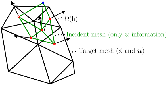
Figure 1: Relevant quantities for the definition of a contact discretization for element $e$.

The modifications required for a classical nonlinear Finite Element software (in our case SimPlas [48]) to include this contact algorithm are modest. Algorithm 1 presents the main tasks. In this Algorithm, blue boxes denote the contact detection task, which here is limited to:

1. Detect nearest neighbor (in terms of distance) elements for each node. A bucket ordering is adopted.

2. Find if the node is interior to any of the neighbor elements by use of the shape functions for triangles and tetrahedra. This is performed in closed form.

3. If changes occurred in the targets, update the connectivity table and the sparse matrix addressing. Gustavson’s algorithm [49] is adopted to perform the updating in the assembling process.

In terms of detection, the following algorithm is adopted:

1. Find all exterior faces, as faces sharing only one tetrahedron.

2. Find all exterior nodes, as nodes belonging to exterior faces.

3. Insert all continuum elements and all exterior nodes in two bucket lists. Deformed coordinates of nodes and deformed coordinates of element centroids are considered.

4. Cycle through all exterior nodes

   1. Determine the element bucket from the node coordinates

   2. Cycle through all elements ($e$) in the $3^{3}=27$ buckets surrounding the node

      1. If the distance from the node to the element centroid is greater than twice the edge size, go to the next element

      2. Calculates the projection on the element ($\bm{\xi}_{I}$) and the corresponding shape functions $\bm{N}\left(\bm{\xi}_{I}\right)$.

      3. If $0\leq N_{K}\left(\bm{\xi}_{I}\right)\leq 1$ then $e$ is the target element. If the target element has changed, then flag the solver for connectivity update.

Since the algorithm assumes a fixed connectivity table during Newton iterations, a verification is required after each converged iteration to check if targets have changed since last determined. If this occurs, a new iteration sequence with revised targets is performed.

Algorithm 1 Staggered contact algorithm based on the approximate distance function. $\lambda$ is the load/displacement factor.

The only modification required to a classical FEM code is the solution of the screened-Poisson equation, the green box in Algorithm 1. The cost of this solution is negligible when compared with the nonlinear solution process since the equation is linear and scalar. It is equivalent to the cost of a steady-state heat conduction solution. Note that this corresponds to a staggered algorithm.

5 Numerical tests

Numerical examples are solved with our in-house software, SimPlas [48], using the new node-to-element contact element. Only triangles and tetrahedra are assessed at this time, which provide an exact solution for $\bm{\xi}_{I}$. Mathematica [47] with the add-on Acegen [46] is employed to obtain the specific source code. All runs are quasi-static and make use of a Neo-Hookean model. If $\bm{C}$ is the right Cauchy-Green tensor, then

$$\bm{S}=2\nicefrac{{\mathrm{d}\psi\left(\bm{C}\right)}}{{\mathrm{d}\bm{C}}}$$

where $\psi\left(\bm{C}\right)=\frac{\mu}{2}\left(\bm{C}:\bm{I}-3\right)-\mu\log\left(\sqrt{\det\bm{C}}\right)+\frac{\chi}{2}\log^{2}\left(\sqrt{\det\bm{C}}\right)$ with $\mu=\frac{E}{2(1+\nu)}$ and $\chi=\frac{E\nu}{(1+\nu)(1-2\nu)}$ being constitutive properties.

Patch test satisfaction

We employ a corrected penalty so that the contact patch test is satisfied in most cases. This is an important subject for convergence of computational contact solutions and has been addressed here with a similar solution to the one discussed by Zavarise and co-workers [17, 16].

We remark that this is not a general solution and in some cases, our formulation may fail to pass the patch test. Figure 2 shows the effect of using a penalty weighted by the edge projection, see [16]. However, this is not an universal solution.

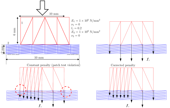
Figure 2: Patch test satisfaction by using a corrected penalty.

5.1 Two-dimensional compression

We begin with a quasi-static two-dimensional test, as shown in Figure 3, using three-node triangles. This test consists of a compression of four polygons (identified as part 3) in Figure 3 by a deformable rectangular punch (part 1 in the same Figure). The ‘U’ (part 2) is considered rigid but still participates in the approximate distance function (ADF) calculation. To avoid an underdetermined system, a small damping term is used, specifically $40$ units with $\mathsf{L}^{-2}\mathsf{M}\mathsf{T}^{-1}$ ISQ dimensions. Algorithm 1 is adopted with a pseudo-time increment of $\Delta t=0.003$ for $t\in[0,1]$.

For $h=0.020$, $h=0.015$ and $h=0.010$, Figure 4 shows a sequence of deformed meshes and the contour plot of $\phi(\bm{x})$. The robustness of the algorithm is excellent, at the cost of some interference for coarse meshes. To further inspect the interference, the contour lines for $g(\bm{x})$ are shown in Figure 5. We note that coarser meshes produce smoothed-out vertex representation, which causes the interference displayed in Figure 4. Note that $g(\bm{x})$ is determined from $\phi(\bm{x})$.

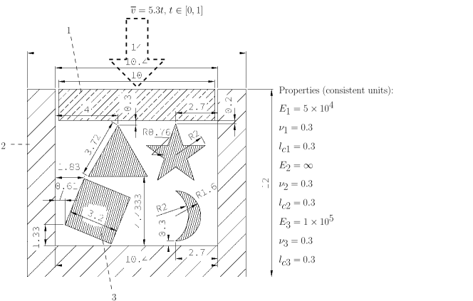
Figure 3: Two-dimensional verification problem. Consistent units are used.

$\overline{v}=0.00$
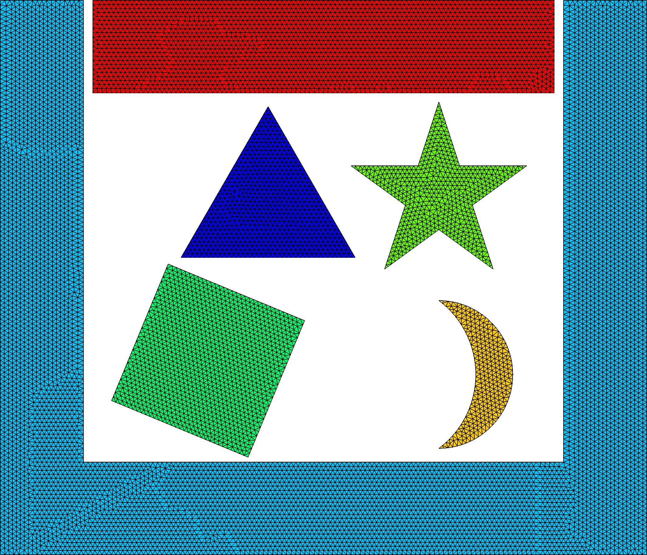
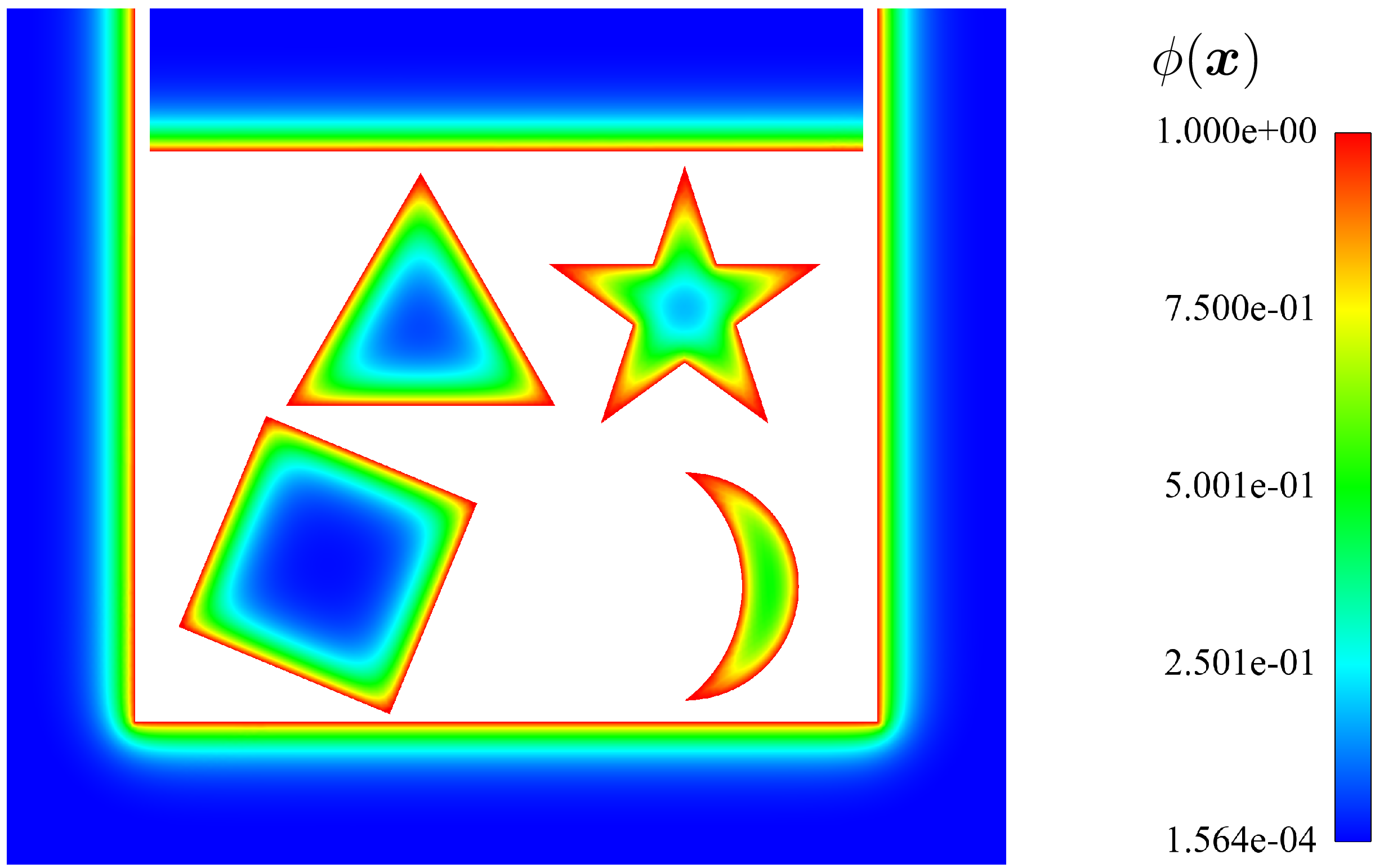
	$\overline{v}=3.24$	$\overline{v}=5.30$	$\overline{v}=5.30$, $\phi$
$h=0.020$
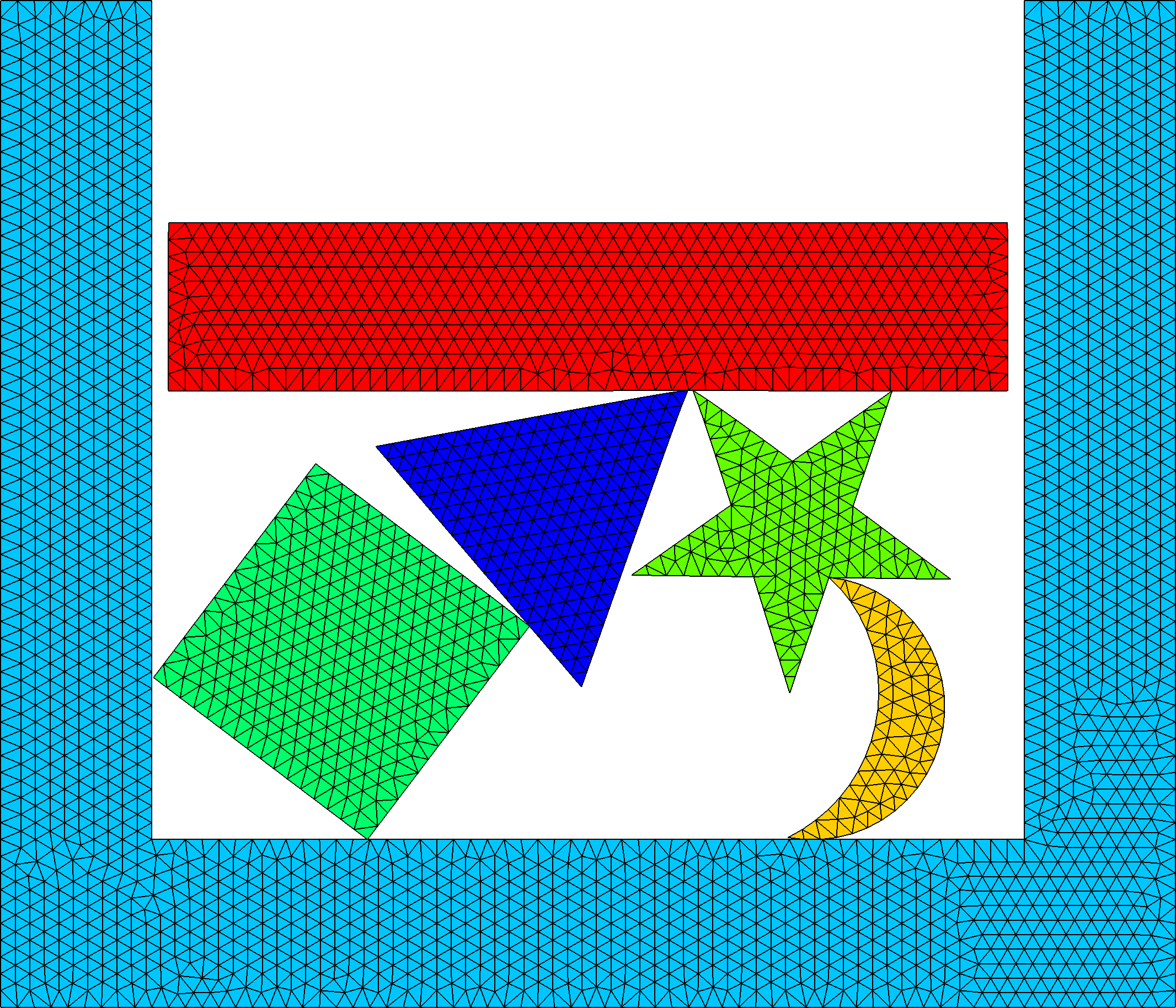
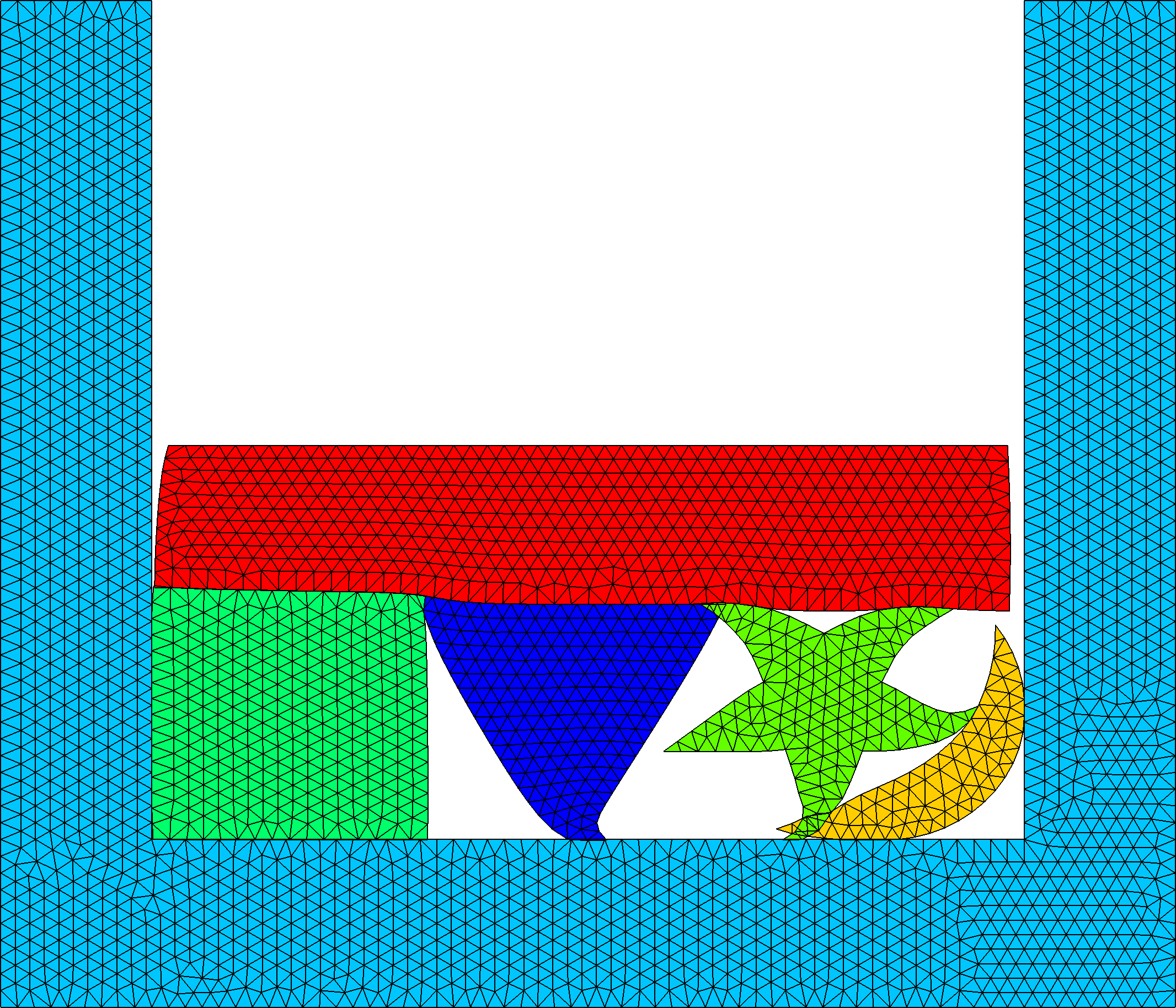
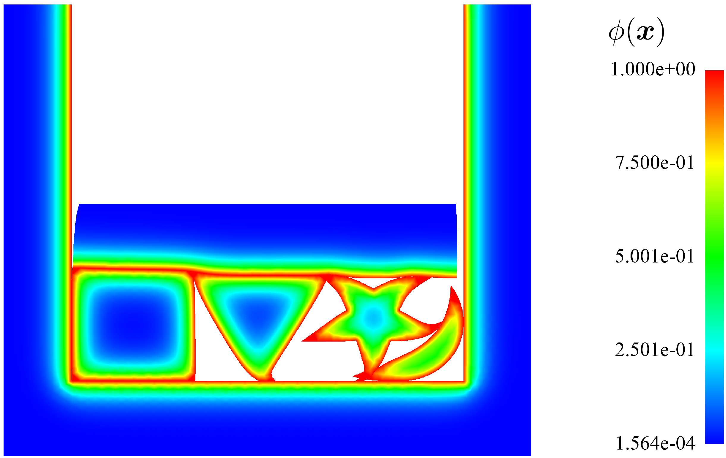
$h=0.015$
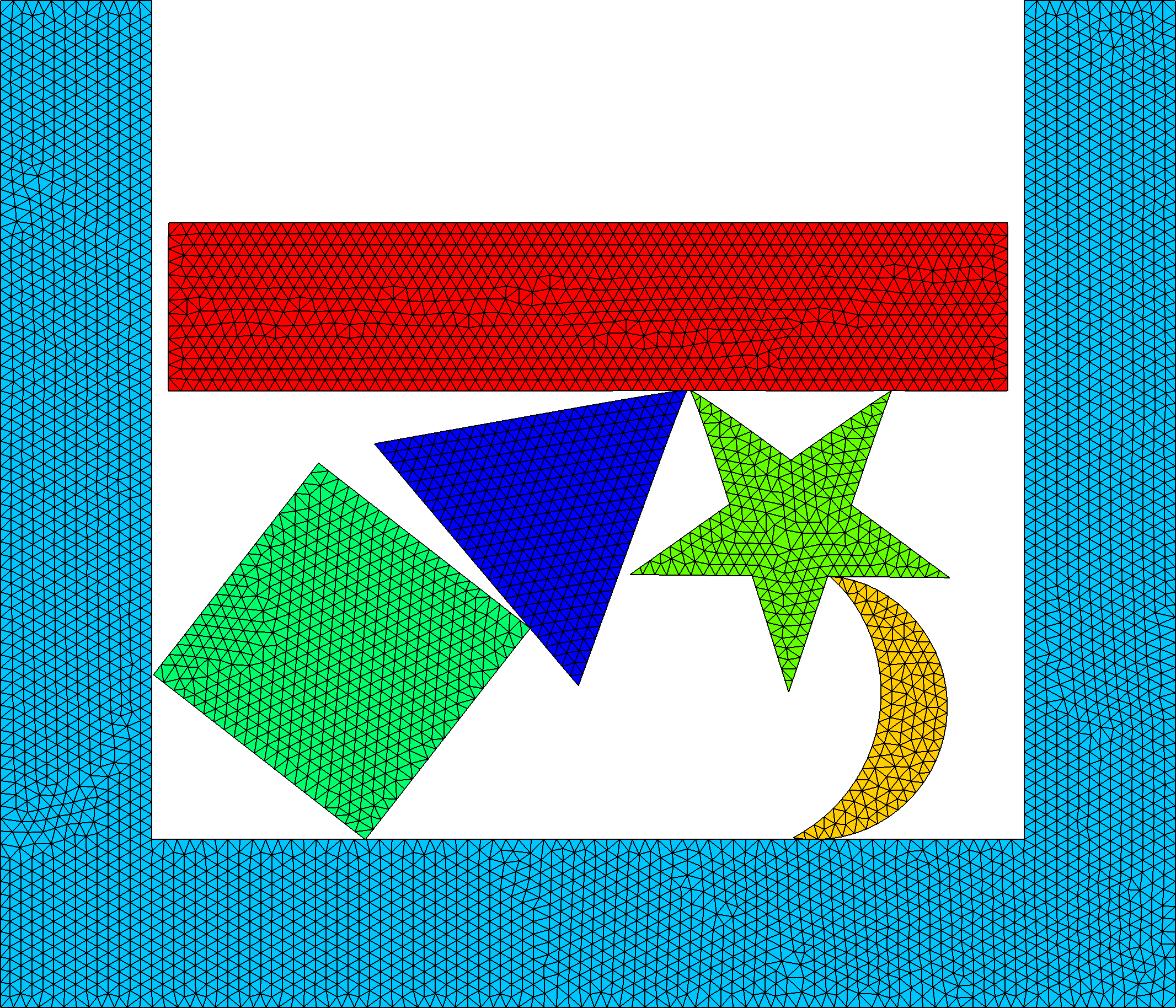
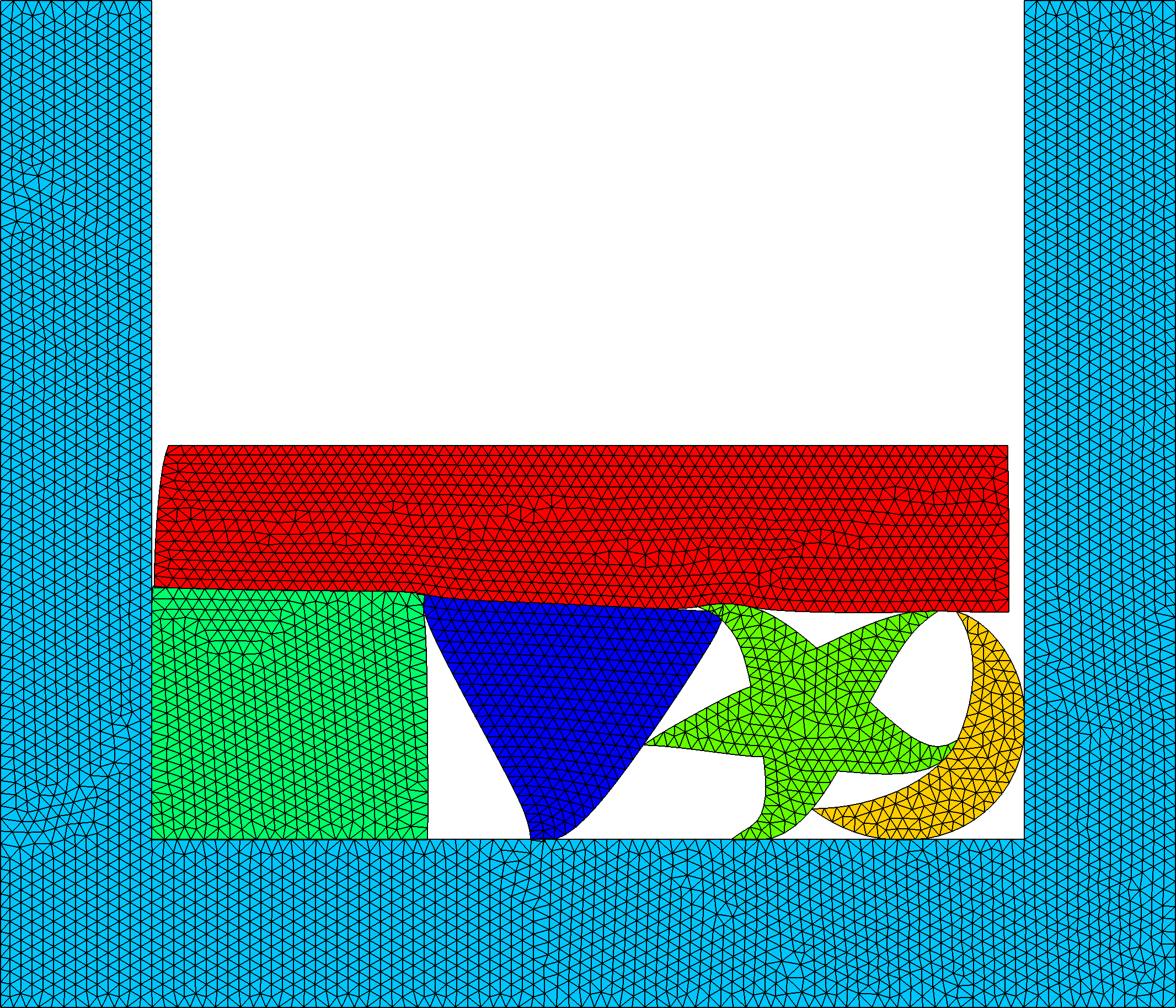
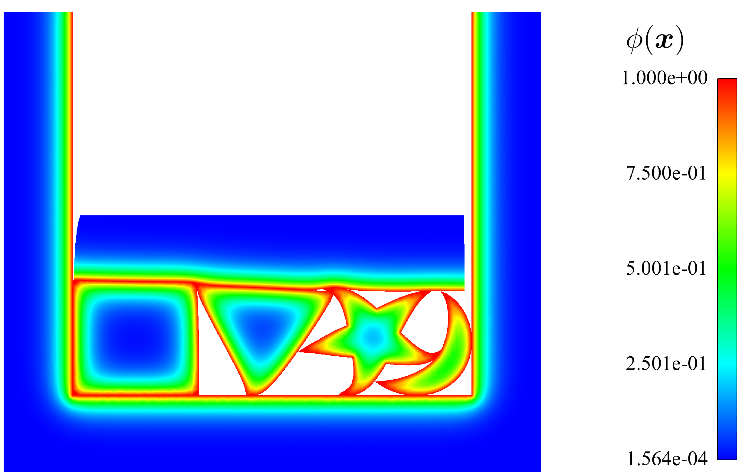
$h=0.010$

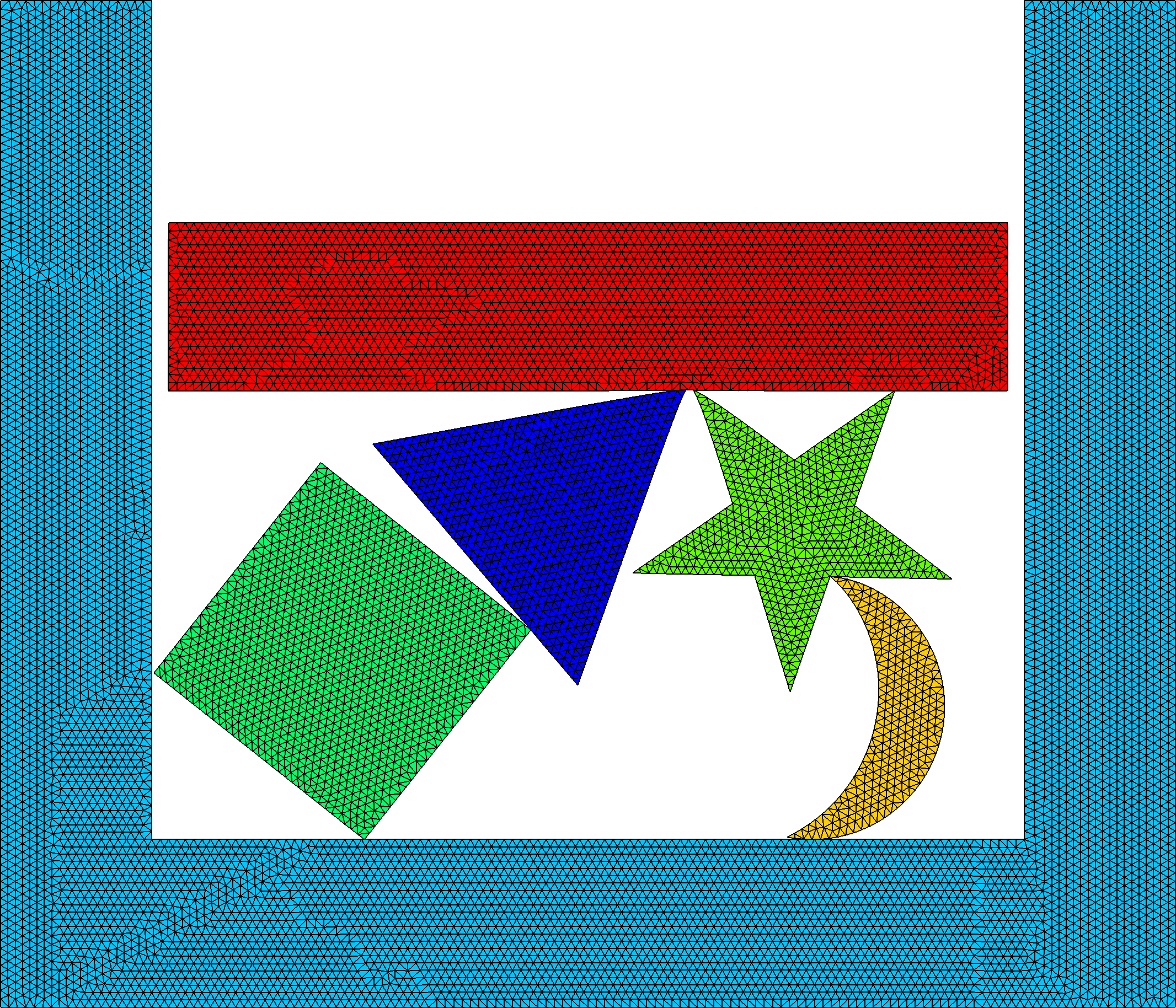
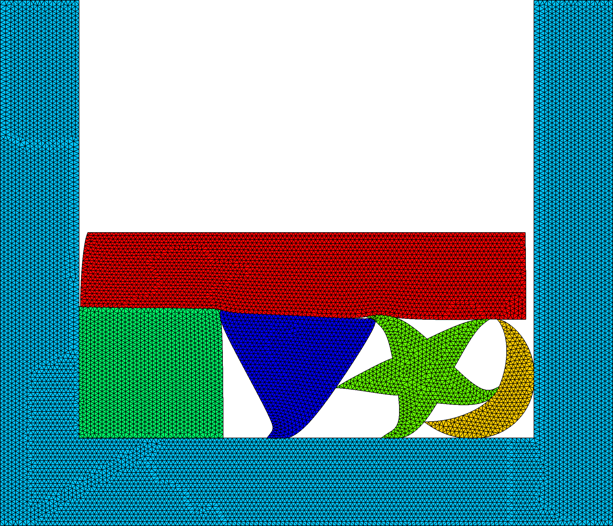
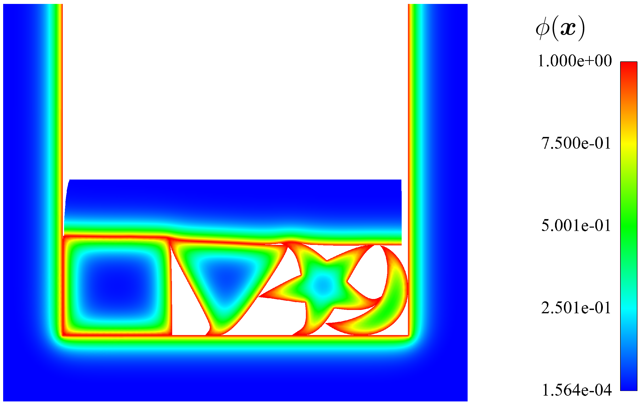
Figure 4: Two-dimensional compression: sequence of deformed meshes and contour plot of $\phi(\bm{x})$.

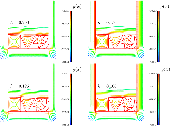
Figure 5: Gap ($g(\bm{x})$) contour lines for the four meshes using $l_{c}=0.3$ consistent units.

Using the gradient of $\phi\left(\bm{x}\right)$, the contact direction is obtained for $h=0.02$ as shown in Figure 6. We can observe that for the star-shaped figure, vertices are poorly represented, since small gradients are present due to uniformity of $\phi\left(\bm{x}\right)$ in these regions. The effect of mesh refinement is clear, with finer meshes producing a sharper growth of reaction when all four objects are in contact with each other. In contrast, the effect of the characteristic length $l_{c}$ is not noticeable.

In terms of the effect of $l_{c}$ on the fields $\phi(\bm{x})$ and $g(\bm{x})$, Figure 7 shows that information, although $\phi(\bm{x})$ is strongly affected by the length parameter, $g(\bm{x})$ shows very similar spatial distributions although different peaks. Effects of $h$ and $l_{c}$ in the displacement/reaction behavior is shown in Figure 8. The mesh size $h$ has a marked effect on the results up to $h=0.0125$, the effect of $l_{c}$ is much weaker.

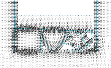
(a) $h=0.020$

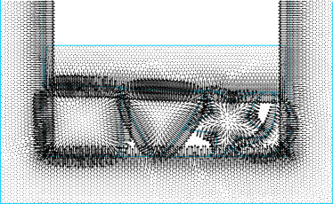
(b) $h=0.015$

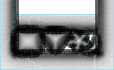
(c) $h=0.010$

Figure 6: Directions obtained as $\nabla\phi\left(\bm{\xi}\right)$ for $h=0.020,$ $0.015$ and $0.010$.

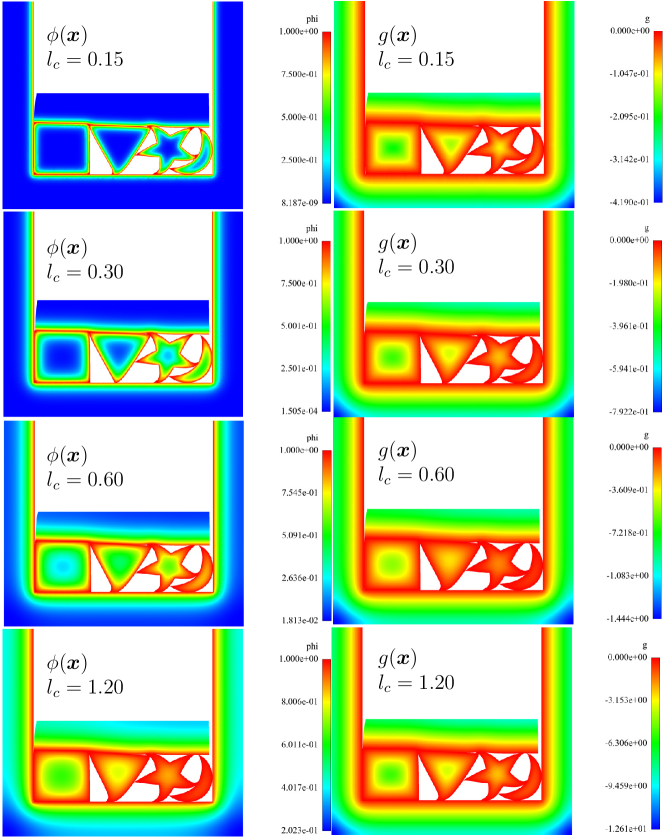
Figure 7: Effect of $l_{c}$ in the form of $\phi(\bm{x})$ and $g(\bm{x})$.

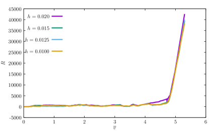
(a)

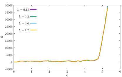
(b)

Figure 8: Effect of $h$ in (a) and effect of $l_{c}$ in (b) in the displacement/reaction behavior.

5.2 Three-dimensional compression

In three dimensions, the algorithm is in essence the same. Compared with geometric-based algorithms, it significantly reduces the coding for the treatment of particular cases (node-to-vertex, node-to-edge in both convex and non-convex arrangements). The determination of coordinates for each incident node is now performed on each tetrahedra, but the remaining tasks remain unaltered. We test the geometry shown in Figure 9 with the following objectives:

• Assess the extension to the 3D case. Geometrical nonsmoothness is introduced with a cone and a wedge.

• Quantify interference as a function of $l_{c}$ and $\kappa$ as well as the strain energy evolution.

Deformed configurations and contour plots of $\phi\left(\bm{x}\right)$ for this problem are presented in Figure 9, and the corresponding CAD files are available on Github [45]. A cylinder, a cone and a wedge are compressed between two blocks. Dimensions of the upper and lower blocks are $10\times 12\times 2$ consistent units (the upper block is deformable whereas the lower block is rigid) and initial distance between blocks is $8$ consistent units. Length and diameter of the cylinder are $7.15$ and $2.86$ (consistent units), respectively. The cone has a height of $3.27$ consistent units and a radius of $1.87$. Finally, the wedge has a width of $3.2$, a radius of $3.2$ and a swept angle of $30$ degrees. A compressible Neo-Hookean law is adopted with the following properties:

• Blocks: $E=5\times 10^{4}$ and $\nu=0.3$.

• Cylinder, cone and wedge: $E=1\times 10^{5}$ and $\nu=0.3$.

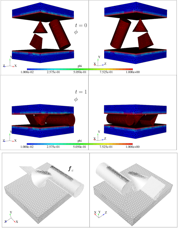
(a)

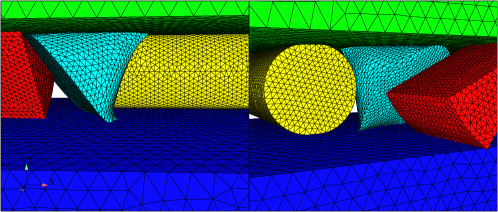
(b)

Figure 9: Data for the three-dimensional compression test. (a) Undeformed and deformed configurations ($h=0.025$). For geometric files, see [45]. (b) Detail of contact of cone with lower block and with the wedge. Each object is identified by a different color.

The analysis of gap violation, $v_{\max}=\sup_{\bm{x}\in\Omega}\left[-\min\left(0,g\right)\right]$ as a function of pseudotime $t\in[0,1]$ is especially important for assessing the robustness of the algorithm with respect to parameters $l_{c}$ and $\kappa$. For the interval $l_{c}\in[0.05,0.4]$, the effect of $l_{c}$ is not significant, as can be observed in Figure 10. Some spikes are noticeable around $t=0.275$ for $l_{c}=0.100$ when the wedge penetrates the cone. Since $\kappa$ is constant, all objects are compressed towards end of the simulation, which the gap violation. In terms of $\kappa$, effects are the same as in classical geometric-based contact. In terms of strain energy, higher values of $l_{c}$ result in lower values of strain energy. This is to be expected, since smaller gradient values are obtained and the contact force herein is proportional to the product of the gradient and the penalty parameter. Convergence for the strain energy as a function of $h$ is presented in Figure 11. It is noticeable that $l_{c}$ has a marked effect near the end of the compression, since it affects the contact force.

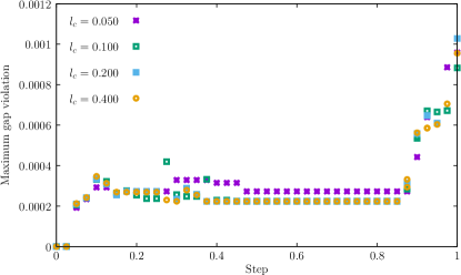
(a)

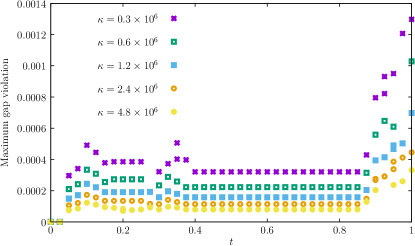
(b)

Figure 10: (a) Effect of $l_{c}$ on the maximum gap evolution over pseudotime $(\kappa=0.6\times 10^{6}$, $h=0.030)$ and (b) Effect of $\kappa$ on the maximum gap evolution over pseudotime $(l_{c}=0.2$).

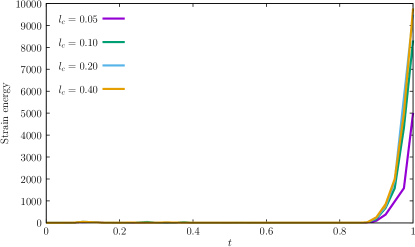
(a)

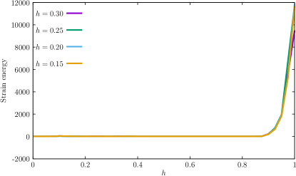
(b)

Figure 11: (a) Effect of $l_{c}$ on the strain energy ($h=0.3$) and (b) Effect of $h$ on the strain energy $(l_{c}=0.2$). $\kappa=0.6\times 10^{6}$ is used.

5.3 Two-dimensional ironing benchmark

This problem was proposed by Yang et al. [50] in the context of surface-to-surface mortar discretizations. Figure 12 shows the relevant geometric and constitutive data, according to [50] and [51]. We compare the present approach with the results of these two studies in Figure 13. Differences exist in the magnitude of forces, and we infer that this is due to the continuum finite element technology. We use finite strain triangular elements with a compressible neo-Hookean law [52]. The effect of $l_{c}$ is observed in Figure 13. As before, only a slight effect is noted in the reaction forces. We use the one-pass version of our algorithm, where the square indenter has the master nodes and targets are all elements in the rectangle. Note that, since the cited work includes friction, we use here a simple model based on regularized tangential law with a friction coefficient, $\mu_{f}=0.3$.

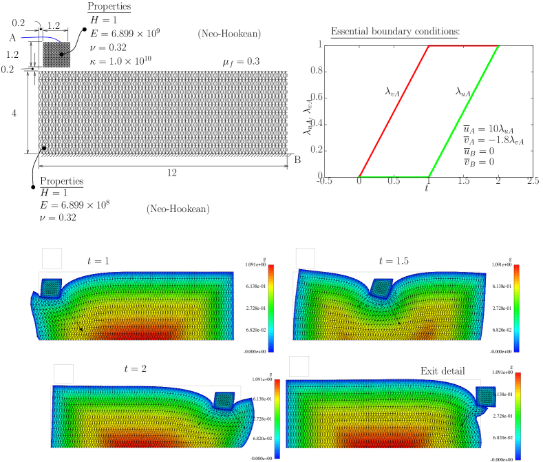
Figure 12: Ironing benchmark in 2D: relevant data and deformed mesh snapshots.

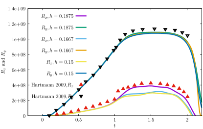
(a)

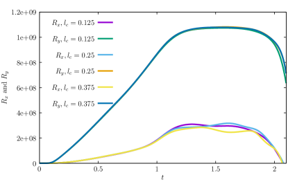
(b)

Figure 13: Ironing problem in 2D. Results for the load in terms of pseudotime are compared to the values reported in Yang et al. [50] and Hartmann et al. [51]. $\kappa=0.6\times 10^{6}$ is used. (a) Effect of $h$ in the evolution of the horizontal ($R_{x}$) and vertical ($R_{y}$) reactions and (b) Effect of $l_{c}$ in the evolution of the horizontal ($R_{x}$) and vertical ($R_{y}$) reactions for $h=0.1667$).

5.4 Three-dimensional ironing benchmark

We now perform a test of a cubic indenter on a soft block. This problem was proposed by Puso and Laursen [18, 19] to assess a mortar formulation based on averaged normals. The frictionless version is adopted [19], but we choose the most demanding case: $\nu=0.499$ and the cubic indenter. Relevant data is presented in Figure 14. The rigid $1\times 1\times 1$ block is located at $1$ unit from the edge and is first moved down $1.4$ units. After this, it moves longitudinally $4$ units inside the soft block. The soft block is analyzed with two distinct meshes: $4\times 6\times 20$ divisions and $8\times 12\times 40$ divisions. Use is made of one plane of symmetry. A comparison with the vertical force in [19] is performed (see also [18] for a clarification concerning the force components). We allow some interference to avoid locking with tetrahedra. In [19], Puso and Laursen employed mixed hexahedra, which are more flexible than the crossed-tetrahedra we adopt here. Figure 15 shows the comparison between the proposed approach and the mortar method by Puso and Laursen [19]. Oscillations are caused by the normal jumps in gradient of $\phi(\bm{x})$ due to the classical $\mathscr{C}^{0}$ finite-element discretization (between elements). Although the oscillations can be observed, the present approach is simpler than the one in Puso and Laursen.

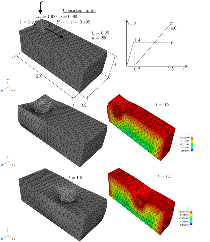
Figure 14: 3D ironing: cube over soft block. Relevant data and results.

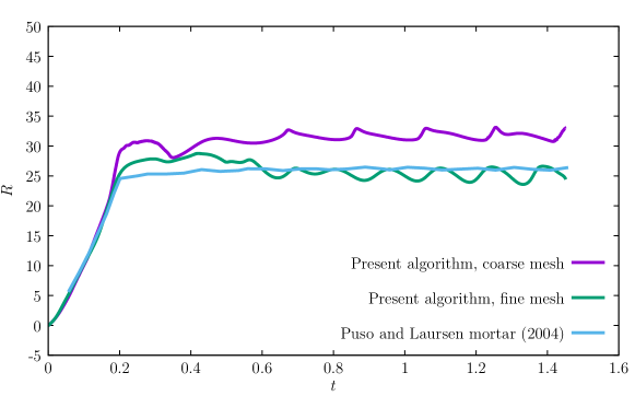
Figure 15: 3D ironing: cube over soft block. Vertical reactions compared with results in Puso and Laursen [19].

6 Conclusions

We introduced a discretization and gap definition for a contact algorithm based on the solution of the screened Poisson equation. After a log-transformation, this is equivalent to the solution of a regularized Eikonal equation and therefore provides a distance to any obstacle or set of obstacles. This approximate distance function is smooth and is differentiated to obtain the contact force. This is combined with a Courant–Beltrami penalty to ensure a differentiable force along the normal direction. These two features are combined with a step-control algorithm that ensures a stable target-element identification. The algorithm avoids most of the geometrical calculations and housekeeping, and is able to solve problems with nonsmooth geometry. Very robust behavior is observed and two difficult ironing benchmarks (2D and 3D) are solved with success. Concerning the selection of the length-scale parameter $l_{c}$, which produces an exact solution for $l_{c}=0$, we found that it should be the smallest value that is compatible with the solution of the screened Poisson equation. Too small of a $l_{c}$ will produce poor results for $\phi\left(\bm{x}\right)$. Newton-Raphson convergence was found to be stable, as well as nearly independent of $l_{c}$. In terms of further developments, a $\mathscr{C}^{2}$ meshless discretization is important to reduce the oscillations caused by normal jumps and we plan to adopt the cone projection method developed in [7] for frictional problems.

References

- [1] N. Sukumar and A. Srivastava. Exact imposition of boundary conditions with distance functions in physics-informed deep neural networks. Comp Method Appl M, 389:114333, 2022.
- [2] Z. Lai, S. Zhao, J. Zhao, and L. Huang. Signed distance field framework for unified DEM modeling of granular media with arbitrary particle shapes. Comput Mech, 70:763–783, 2022.
- [3] P. Wriggers. Computational Contact Mechanics. John Wiley and Sons, New York, 2002.
- [4] J. Simo and T. Laursen. An augmented Lagrangian treatment of contact problems involving friction. Comput Struct, 42:97–116, 1992.
- [5] J. Nitsche. Über ein Variationsprinzip zur Lösung von Dirichlet-Problemen bei Verwendung von Teilräumen, die keinen Randbedingungen unterworfen sind. Abhandlungen in der Mathematik an der Universitẗ Hamburg, 36:9–15, 1970.
- [6] Y. Kanno, J.A.C. Martins, and A. Pinto da Costa. Three-dimensional quasi-static frictional contact by using second-order cone linear complementarity problem. Int J Numer Meth Eng, 65:62–83, 2006.
- [7] P. Areias, T. Rabczuk, and F.J.M.Q. de Melo. Coulomb frictional contact by explicit projection in the cone for finite displacement quasi-static problems. Comput Mech, 55:57–72, 2015.
- [8] T.A. Laursen and J.C. Simo. Algorithmic symmetrization of coulomb frictional problems using augmented lagrangians. Comp Method Appl M, 108:133–146, 1993.
- [9] G. De Saxcé and Z.-Q. Feng. The bipotential method: A constructive approach to design the complete contact law with friction and improved numerical algorithms. Mathl Comput Modelling, 28(4-8):225–245, 1998.
- [10] R.E. Jones and P. Papadopoulos. A yield-limited Lagrange multiplier formulation for frictional contact. Int J Numer Meth Eng, 48:1127–1149, 2000.
- [11] J.C. Simo, P. Wriggers, and R.L. Taylor. A perturbed Lagrangian formulation for the finite element solution of contact problems. Comp Method Appl M, 50:163–180, 1985.
- [12] S.K. Chan and I.S. Tuba. A finite element method for contact problems of solid bodies-Part I. Theory and validation. Int J Mech Sci, 13:615–625, 1971.
- [13] A. Francavilla and O.C. Zienkiewicz. A note on numerial computation of elastic contact problems. Int J Numer Meth Eng, 9:913–924, 1975.
- [14] J.O. Hallquist, G.L. Goudreau, and D.J. Benson. Sliding interfaces with contact-impact in large-scale Lagrangian computations. Comp Method Appl M, 51:107–137, 1985.
- [15] D.M. Neto, M.C. Oliveira, L.F. Menezes, and J.L. Alves. Applying Nagata patches to smooth discretized surfaces used in 3D frictional contact problems. Comp Method Appl M, 271:296–320, 2014.
- [16] G. Zavarise and L. De Lorenzis. A modified node-to-segment algorithm passing the contact patch test. Int J Numer Meth Eng, 79:379–416, 2009.
- [17] G. Zavarise and L. De Lorenzis. The node-to-segment algorithm for 2D frictionless contact: Classical formulation and special cases. Comp Method Appl M, 198:3428–3451, 2009.
- [18] M.A. Puso and T.A. Laursen. A mortar segment-to-segment frictional contact method for large deformations. Comp Method Appl M, 193:4891–4913, 2004.
- [19] M.A. Puso and T.A. Laursen. A mortar segment-to-segment contact method for large deformation solid mechanics. Comp Method Appl M, 193:601–629, 2004.
- [20] G. Zavarise and P. Wriggers. A segment-to-segment contact strategy. Mathl Comput Modelling, 28(4-8):497–515, 1998.
- [21] C. Kim, R.D. Lazarov, J.E. Pasciak, and P.S. Vassilevski. Multiplier spaces for the mortar finite element method in three dimensions. SIAM J Numer Anal, 39(2):519–538, 2001.
- [22] T.A. Laursen, M.A. Puso, and J. Sanders. Mortar contact formulations for deformable-deformable contact: Past contributions and new extensions for enriched and embedded interfance formulations. Comp Method Appl M, 205-208:3–15, 2012.
- [23] P. Farah, A. Wall, and A. Popp. A mortar finite element approach for point, line and surface contact. Int J Numer Meth Eng, 114:255–291, 2018.
- [24] P. Wriggers, J. Schröder, and A. Schwarz. A finite element method for contact using a third medium. Comput Mech, 52:837–847, 2013.
- [25] C. Kane, E.A. Repetto, M. Ortiz, and J.E. Marsden. Finite element analysis of nonsmooth contact. Comp Method Appl M, 180:1–26, 1999.
- [26] P. Litewka. Enhanced multiple-point beam-to-beam frictionless contact finite element. Comput Mech, 52:1365–1380, 2013.
- [27] A.G. Neto, P.M. Pimenta, and P. Wriggers. A master-surface to master-surface formulation for beam to beam contact. Part I: frictionless interaction. Comp Method Appl M, 303:400–429, 2016.
- [28] A.G. Neto, P.M. Pimenta, and P. Wriggers. A master-surface to master-surface formulation for beam to beam contact. Part II: Frictional interaction. Comp Method Appl M, 319:146–174, 2017.
- [29] C. Meier, W.A. Wall, and A. Popp. A unified approach for beam-to-beam contact. Comp Method Appl M, 315:972–1010, 2017.
- [30] S. Wolff and C. Bucher. Distance fields on unstructured grids: stable interpolation, assumed gradients, collision detection and gap function. Comp Method Appl M, 259:77–92, 2013.
- [31] X. Liu, J. Mao, L. Zhao, L. Shao, and T. Li. The distance potential function-based finite-discrete element method. Comput Mech, 66:1477–1495, 2020.
- [32] M. Aguirre and S. Avril. An implicit 3D corotational formulation for frictional contact dynamics of beams against rigid surfaces using discrete signed distance fields. Comp Method Appl M, 371:113275, 2020.
- [33] M. Macklin, K. Erleben, M. Müller, N. Chentanez, S. Jeschke, and Z. Corse. Local optimization for robust signed distance field collision. Proc ACM Comput Graph Interact Tech, 3(1):1–9, 2020.
- [34] A.G. Belyaev and P.-A. Fayolle. On variational and PDE-based distance function approximations. Comput Graph Forum, 34(8):104–118, 2015.
- [35] K. Crane, C. Weischedel, and M. Wardetzky. Geodesics in heat: A new approach to computing distance based on heat flow. ACM Trans Graph, 32(5):Art 152, 2013.
- [36] R.H.J. Peerlings, R. de Borst, W.A.M. Brekelmans, and J.H.P. de Vree. Gradient enhanced damage for quasi-brittle materials. International Journal for Numerical Methods in Engineering, 39:3391–3403, 1996.
- [37] R.H.J. Peerlings, W.A.M. Brekelmans, R. de Borst, and M.G.D. Geers. Mathematical and numerical aspects of an elasticity-based local approach to fracture. Revue Europeenne des Elements Finis, 10:209–226, 2001.
- [38] R.A. Guler, S. Tari, and G. Unal. Screened Poisson hyperfields for shape coding. SIAM J Imaging Sciences, 7(4):2558–2590, 2014.
- [39] A. Belyaev and P.-A. Fayolle. An ADMM-based scheme for distance function approximation. Numer Algorithms, 84:983–996, 2020.
- [40] A. Konyukhov and K. Schweizerhof. On the solvability of closest point projection procedures in contact analysis: analysis and solution strategy for surfaces of arbitrary geometry. Comp Method Appl M, 197(33-40):3045–3056, 2008.
- [41] G. Russo and P. Smereka. A remark on computing distance functions. J Comput Phys, 163:51–67, 2000.
- [42] R. Courant. Variational methods for the solution of problems of equilibrium and vibrations. Bull Am Math Soc, 49:1–23, 1943.
- [43] E.J. Beltrami. A constructive proof of the kuhn-tucker multiplier rule. J Math Anal Appl, 26:297–306, 1969.
- [44] S.R.S. Varadhan. On the behavior of the fundamental solution of the heat equation with variable coefficients. Comm Pure Appl Math, XX:431–455, 1967.
- [45] P. Areias. 3D contact files. https://github.com/PedroAreiasIST/contact3d, 2022.
- [46] J. Korelc. Multi-language and multi-environment generation of nonlinear finite element codes. Eng Computers, 18(4):312–327, 2002.
- [47] Wolfram Research Inc. Mathematica, 2007.
- [48] P. Areias. Simplas. http://www.simplassoftware.com. Portuguese Software Association (ASSOFT) Registry number 2281/D/17.
- [49] F.G. Gustavson. Two fast algorithms for sparse matrices: multiplication and permuted transposition. Trans Math Soft-ACM, 4(3):250–269, 1978.
- [50] B. Yang, T.A. Laursen, and X. Meng. Two dimensional mortar contact methods for large deformation frictional sliding. Int J Numer Meth Eng, 62:1183–1225, 2005.
- [51] S. Hartmann, J. Oliver, R. Weyler, J.C. Cante, and J.A. Hernández. A contact domain method for large deformation frictional contact problems. Part 2: Numerical aspects. Comp Method Appl M, 198:2607–2631, 2009.
- [52] J. Bonet and R.D. Wood. Nonlinear Continuum Mechanics for Finite Element Analysis. Cambridge University Press, Second edition, 2008.