Leaking from the phase space of the
Riemann-Liouville fractional standard map

Abstract

In this work we characterize the escape of orbits from the phase space of the Riemann-Liouville (RL) fractional standard map (fSM). The RL-fSM, given in action-angle variables, is derived from the equation of motion of the kicked rotor when the second order derivative is substituted by a RL derivative of fractional order $\alpha$. Thus, the RL-fSM is parameterized by $K$ and $\alpha\in(1,2]$ which control the strength of nonlinearity and the fractional order of the RL derivative, respectively. Indeed, for $\alpha=2$ and given initial conditions, the RL-fSM reproduces Chirikov’s standard map. By computing the survival probability $P_{\text{S}}(n)$ and the frequency of escape $P_{\text{E}}(n)$, for a hole of hight $h$ placed in the action axis, we observe two scenarios: When the phase space is ergodic, both scattering functions are scale invariant with the typical escape time $n_{\text{typ}}=\exp\langle\ln n\rangle\propto(h/K)^{2}$. In contrast, when the phase space is not ergodic, the scattering functions show a clear non-universal and parameter-dependent behavior.

1 Introduction

When discussing about the generic transition to chaos, in the context of the Kolmogorov–Arnold–Moser (KAM) theorem, probably one of the most popular example models is the kicked rotor (KR); see e.g. [1]. The KR, which represents a free rotating stick in an inhomogeneous field that is periodically switched on in instantaneous pulses, is described by the second order differential equation

$$\ddot{x}+K\sin(x)\sum_{n=0}^{\infty}\delta\left(\frac{t}{T}-n\right)=0.$$ (1)

Here, $x\in[0,2\pi]$ is the angular position of the stick, $K$ is the kicking strength, $T$ is the kicking period (that we set to one from now on), and $\delta$ is Dirac’s delta function. A very useful approach to the dynamics of the KR is by studying its stroboscopic projection, which is well known as Chirikov’s standard map (CSM) [2]:

$$\begin{array}[]{ll}p_{n+1}=p_{n}-K\sin(x_{n}),\\ x_{n+1}=x_{n}+p_{n+1},\qquad\mbox{mod}~{}(2\pi),\\ \end{array}$$ (2)

where $p$ corresponds to the angular momentum of the KR’s stick. Indeed, CSM is known to represent the local dynamics of several Hamiltonian systems and is by itself a paradigm model of the KAM scenario.

In order to account for dynamical features not present in KAM’s scenario, modified versions of CSM have been introduced. Among them we can highlight the dissipative version of CSM (also known as Zaslavsky map) [3] and the discontinuous version of CSM [4]. Moreover, by substituting the second-order derivative in the equation of the KR by the Riemann-Liouville (RL) derivative ${}_{0}D_{t}^{\alpha}$, the RL fractional KR is obtained [5, 6]:

$${}_{0}D_{t}^{\alpha}x+K\sin(x)\sum_{n=0}^{\infty}\delta\left(t-n\right)=0,\quad 1<\alpha\leq 2.$$ (3)

Above

$${}_{0}D_{t}^{\alpha}x(t)=D_{t}^{m}{{}_{0}I}_{t}^{m-\alpha}x(t)$$

$$=\frac{1}{\Gamma(m-\alpha)}\frac{d^{m}}{dt^{m}}\int_{0}^{t}\frac{x^{\tau}d\tau}{(t-\tau)^{\alpha-m+1}},\quad m-1<\alpha\leq m,$$

with $D_{t}^{m}=d^{m}/dt^{m}$ and ${}_{0}I_{t}^{m}f(t)$ is a fractional integral given by

$${}_{0}I_{t}^{m}f(t)=\frac{1}{\Gamma(m)}\int_{0}^{t}(t-\tau)^{\alpha-1}f(\tau)d\tau.$$

Notice that now $p(t)\equiv{{}_{0}D}_{t}^{\alpha-1}x(t)$.

Correspondingly, the stroboscopic projection of the RL fractional KR is known as the RL fractional standard map (RL-fSM) which reads as [6]

$$\begin{array}[]{ll}p_{n+1}=p_{n}-K\sin(x_{n}),\\ x_{n+1}=\displaystyle{\frac{1}{\Gamma(\alpha)}\sum_{i=0}^{n}p_{i+1}V_{\alpha}(n-i+1)}\\ \qquad\quad\displaystyle{+\frac{b}{\Gamma(\alpha-1)}(n+1)^{\alpha-2},\quad\mbox{mod}~{}(2\pi).}\end{array}$$ (4)

Here, $\Gamma$ is the Gamma function and

$$V_{\alpha}(m)=m^{\alpha-1}-(m-1)^{\alpha-1}.$$

Note that the sum in the equation for the position in map (4) makes the RL-fSM to have memory, meaning that the future $(n+1)$–state depends on the entire orbit and not on the present $n$–state only. The property of memory is known to be present in maps derived from fractional differential equations [7], such as the RL-fSM of Eq. (4), but also in maps derived from fractional integral equations [8] and in maps derived from fractional integro-differential equations [9].

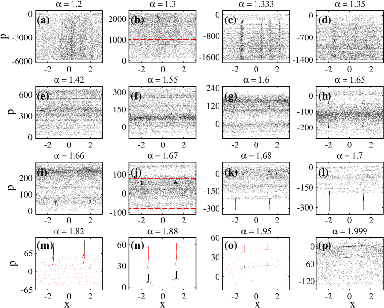
Figure 1: Poincaré surfaces of section for the Riemann-Liouville fractional standard map of Eq. (5) with $K=4.6$ and several values of $\alpha$. A single initial condition with $x_{0}=0$ and a random $p_{0}\in(0,2\pi/100)$ was iterated $10^{4}$ times (black dots). Red dots in panels (m,n,o) represent the orbit of a second initial condition. Holes in the action axis in panels (b,c,j) are located at $p=\pm h$ (red dashed lines) with $h=1000$, 800 and 80, respectively.

It is important to add that for $b=0$, in the case $\alpha=2$, the RL-fSM reproduces CSM. Therefore in this work we consider the RL-fSM in the form

$$\begin{array}[]{ll}p_{n+1}=p_{n}-K\sin(x_{n}),\\ x_{n+1}=\displaystyle{\frac{1}{\Gamma(\alpha)}\sum_{i=0}^{n}p_{i+1}V_{\alpha}(n-i+1)},\quad\mbox{mod}~{}(2\pi),\end{array}$$ (5)

where $1<\alpha\leq 2$ is assumed. The RL-fSM has no periodicity in $p$ and cannot be considered on a torus like CSM.

In contrast with CSM, depending on the strength of nonlinearity $K$ and the fractional order of the RL derivative $\alpha$, the RL-fSM generates attractors (fixed points, asymptotically stable periodic trajectories, slow converging and slow diverging trajectories, ballistic trajectories, and fractal-like structures) and/or chaotic trajectories [6, 10, 11]. Moreover, trajectories may intersect and attractors may overlap [12]. As an example, in Fig. 1 we present Poincaré surfaces of section for the RL-fSM with $K=4.6$ and several values of $\alpha$. In this figure we can observe the convergence to asymptotically stable periodic trajectories (see the period-two periodic orbits in panels (k) to (o)), the existence of unstable periodic trajectories (see the period-four periodic orbit in panel (c)), as well as quite uniform chaotic trajectories (see panels (a) and (d)). Similar Poincaré surfaces of section are observed for other values of $K$. Thus, we can safely state that the RL-fSM is a richer dynamical system as compared to CSM.

Since its investigation by Edelman and Tarasov [6], several studies on the RL-fSM have been reported and other fractional versions of the standard map have also been introduced, see e. g. [7, 12, 13, 14, 15, 16, 17, 18, 19]. Among those studies we highlight that: Already in Refs. [14, 15] the dissipative fSM (which is the fractional version of Zaslavsky map [3]) was introduced; the Caputo fSM (i.e. the fSM derived from the KR with a Caputo fractional derivative) was introduced and contrasted with the RL-fSM in Ref. [12]; the $\alpha$-family of the fSM, where the order of the fractional derivative is not restricted to $1<\alpha\leq 2$, was defined in Refs. [13, 17, 19].

Coming back to the RL-fSM, even though many of its properties have been already studied, as far as we know, its scattering properties have not been explored yet. Thus, in this work we undertake this task and characterize the escape of orbits from the phase space of the RL-fSM. Specifically, in this work we compute the survival probability $P_{\text{S}}(n)$ and the frequency of escape $P_{\text{E}}(n)$ for a hole of hight $h$ placed in the action axis. Then, we analyze both scattering quantities as a function of $K$ and $\alpha$, the parameters of the RL-fSM.

2 Scattering setup and scattering measures

Scattering experiments are used to probe the properties of target systems by measuring transport or scattering quantities [20]. In classical scattering we can cite two main scattering setups: in one setup particles are measured after they are scattered by a target system while in another setup the target system is characterized by means of particle leaking. Here we use the second setup where the leak can be a physical hole (such as an opening in the boundary of a billiard table) or a subset of the phase space (i.e., a threshold in one or more variables). In either case, an orbit with initial conditions inside the dynamical system that reaches the hole is considered to escape from the system, see e.g. [21, 22, 23]. In studies of classical leaking, the survival probability $P_{S}(n)$ and the frequency of escape $P_{E}(n)$ are widely used quantities; hence, in this work we compute both.

We open the RL-fSM by placing a hole on a subset of the phase space of constant action. Furthermore, we set the hole as two horizontal lines at $p=\pm h$ in the Poincaré surfaces of section; this is due to the symmetry of the phase space around $p=0$, i.e. $\langle p_{n}\rangle=0$. In Figs. 1(b), 1(c) and 1(j) we show examples of holes with $h=1000$, 800 and 80, respectively (see red dashed lines). Thus, controlling the nonlinearity ($K$) of map (5), the fractional order of the RL derivative ($\alpha$), and the openness of the scattering setup ($h$), we analyze the escape of trajectories from the RL-fSM.

For each combination of $(K,h,\alpha)$, we consider an ensemble of $10^{5}$ orbits having as initial conditions $x_{0}=0$ and random $p_{0}$ uniformly distributed in the interval $(0,2\pi/100)$. Trajectories with each initial condition evolve in time according to map (5). Once $|p_{n}|>h$, we conclude that the orbit has escaped from the RL-fSM and choose a new initial condition. We count the number of orbits $N_{\text{S}}(n)$, that at time $n$, have not escaped yet from the RL-fSM, then we compute $P_{\text{S}}(n)$ as $P_{\text{S}}(n)=N_{\text{S}}(n)/M$. While keeping track of the total number of orbits that have escaped up to time $n$, we simultaneously construct a histogram for the frequency of escape $P_{\text{E}}(n)$.

3 Survival probability and frequency of escape

Since the RL-fSM displays a rich and diverse dynamics we characterize the orbits leaking from its phase space first when the phase space is ergodic and later when it is not. Also, without loss of generality, in the following numerical calculations we consider two relatively large values of $K$ (6.908745 and 7.5) which allowed us to get good statistics in reasonable computer times. We note that some aspects of the dynamics of the RL-fSM with $K=6.908745$ have been explored in [6], so we decided to use this value of $K$ in our study. Moreover, we verified that our conclusions do not depend on these values of $K$.

3.1 Ergodic phase space

In Figs. 2(a,b) we present the survival probability $P_{\text{S}}(n)$ as a function of $n$ for the RL-fSM with $K=6.908745$ and several combinations of $\alpha$ and $h$. The values of $\alpha$ we choose in Figs. 2(a,b) produce an ergodic phase space, see Fig. 1; or at least we did not observe the formation of structures in phase space for the values of $h$ we consider. Note that we are considering here the value of $\alpha=2$, see the magenta curves in Fig. 2(b), which corresponds to CSM whose scattering properties have already been studied in [22, 23]. From Figs. 2(a,b) we note that $P_{\text{S}}(n)$ shows an almost perfect exponential decay of the form

$$P_{\text{S}}(n)=\exp\left(-\frac{n}{\mu}\right),$$ (6)

which is typical of strongly chaotic systems [20, 24] (see also [22, 23]). Indeed, the full lines in Figs. 2(a,b) are fittings of Eq. (6) to the data (symbols), were $\mu$ has been used as a fitting parameter.

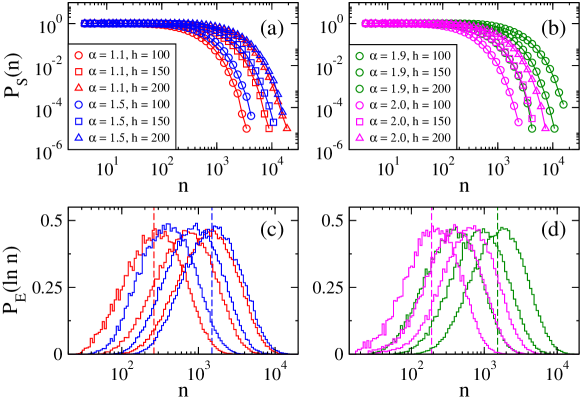
Figure 2: (a,b) Survival probability $P_{\text{S}}(n)$ as a function of $n$ (symbols) for the RL-fSM with $K=6.908745$ and some combinations of $\alpha$ and $h$ ($\alpha=1.1$ in red, $\alpha=1.5$ in blue, $\alpha=1.9$ in green, and $\alpha=2$ in magenta; $h$ grows from left to right, as labeled in the figure). Full lines are fittings of the data with Eq. (6). Curves were computed from $M=10^{5}$ orbits. (c,d) Histograms for the frequency of escape $P_{\text{E}}(\ln n)$. Same color code as in (a,b). The typical escape times $n_{\text{typ}}=\exp\langle\ln n\rangle$ are indicated by the vertical dashed lines (they are shown for four histograms only to avoid figure saturation). Histograms were computed from $M=10^{5}$ orbits.

For the frequency of escape $P_{\text{E}}(n)$, we found that it grows with $n$, reaches a maximum value, and then decreases to zero for exponentially large iteration times. Thus, in order to clearly observe the complete panorama, we compute $P_{\text{E}}(\ln n)$ instead (see also [22, 23]). Therefore, in Figs. 2(c,d) we present $P_{\text{E}}(\ln n)$ for for the RL-fSM with $K=6.908745$ and the same combinations of $\alpha$ and $h$ used in panels (a,b) for $P_{\text{S}}(n)$.

To stress the fact that the panorama shown in Fig. 2 is generic for the RL-fSM when the parameters $K$ and $\alpha$ produce an ergodic phase space, in Fig. 3 we show $P_{\text{S}}(n)$ and $P_{\text{E}}(\ln n)$ now for $K=7.5$ and several different combinations of $\alpha$ and $h$. In Fig. 2 we present the Poincaré surfaces of section corresponding to the chosen values of $\alpha$.

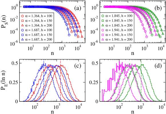
Figure 3: (a,b) Survival probability $P_{\text{S}}(n)$ as a function of $n$ (symbols) for the RL-fSM with $K=7.5$ and some combinations of $\alpha$ and $h$ ($\alpha=1.364$ in red, $\alpha=1.687$ in blue, $\alpha=1.845$ in green, and $\alpha=1.941$ in magenta; $h$ grows from left to right, as labeled in the figure). Full lines are fittings of the data with Eq. (6). Curves were computed from $M=10^{5}$ orbits. (c,d) Histograms for the frequency of escape $P_{\text{E}}(\ln n)$. Same color code as in (a,b). The typical escape times $n_{\text{typ}}=\exp\langle\ln n\rangle$ are indicated by the vertical dashed lines (they are shown for four histograms only to avoid figure saturation). Histograms were computed from $M=10^{5}$ orbits.

In [23], it was shown that the typical iteration time,

$$n_{\text{typ}}=\exp{\left\langle\ln n\right\rangle},$$ (7)

characterizes well the maximum of $P_{\text{E}}(\ln n)$ of strongly chaotic systems. This fact is also valid for the RL-fSM with an ergodic phase space, as can be seen in Figs. 2(c,d) and Figs. 3(c,d) where $n_{\text{typ}}$ is indicated with vertical dashed lines for selected histograms. Moreover, the relation between $P_{\text{E}}(n)$ and $P_{\text{S}}(n)$,

$$P_{\text{E}}(n)=-\frac{dP_{\text{S}}(n)}{dn},$$ (8)

let us state that $\mu=n_{\text{typ}}$ and, accordingly, allows us to write

$$P_{\text{S}}(n)\approx\exp\left(-\frac{n}{n_{\text{typ}}}\right).$$ (9)

Note that in Eq. (9) we are writing approximately equal instead of equal. This is because we numerically found that $\mu\approx n_{\text{typ}}$, as can be seen in the insets of Figs. 4(a,b) where we plot $n_{\text{typ}}$ vs. $\mu$; here $\mu$ is extracted from the fittings of Eq. (6) to the $P_{\text{S}}(n)$ curves of Figs. 2(a,b) and Figs. 3(a,b).

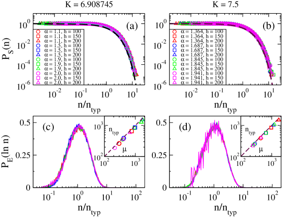
Figure 4: Survival probability $P_{\text{S}}(n)$ as a function of $n/n_{\text{typ}}$ for the RL-fSM with (a) $K=6.908745$ and (b) $K=7.5$; same curves of (a) Figs. 2(a,b) and (b) Figs. 3(a,b). Dashed black lines in (a,b) correspond to Eq. (9). Insets in (c,d) show $n_{\text{typ}}$ vs. $\mu$. The values of $\mu$ were extracted by fitting Eq. (6) to the $P_{\text{S}}(n)$ curves of (a) Figs. 2(a,b) and (b) Figs. 3(a,b). The relation $n_{\text{typ}}=\mu$ (dashed lines) is shown as a reference. Histograms for the frequency of escape $P_{\text{E}}(\ln n)$ as a function of $n/n_{\text{typ}}$ for the RL-fSM with (c) $K=6.908745$ and (d) $K=7.5$; same curves of (c) Fig. 2(c,d) and (d) Fig. 3(c,d).

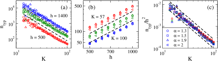
Figure 5: (a) Typical iteration time $n_{\text{typ}}$ as a function of $K$ for the RL-fSM. Here $h=500$ (red symbols), $h=950$ (green symbols), and $h=1400$ (blue symbols); different values of $\alpha$ are shown: $\alpha=1.3$ ($\circ$), $\alpha=1.5$ ($\square$), $\alpha=1.9$ ($\triangle$), and $\alpha=2$ ($\triangleleft$). $n_{\text{typ}}\propto K^{-2}$ (dashed lines) is shown as a reference. (b) $n_{\text{typ}}$ as a function of $h$. $K=57$ (red symbols), $K=76$ (green symbols), and $K=100$ (blue symbols) for the values of $\alpha$ reported in (a). $n_{\text{typ}}\propto h^{2}$ (dashed lines) is shown as a reference. (c) Typical escape time $n_{\text{typ}}$, normalized to $h^{2}$, as a function of $K$. Same data as in panel (a). $n_{\text{typ}}\propto K^{-2}$ (dashed lines) is shown as a reference.

Expression (9) is of paramount importance because it reveals that $P_{\text{S}}(n)$ and accordingly $P_{\text{E}}(\ln n)$ depend on the ratio $n/n_{\text{typ}}$ only; meaning that the typical iteration time (see Eq. (7)) is the scaling parameter of both quantities. In practical terms, this means that when plotting $P_{\text{S}}(n)$ vs. $n/n_{\text{typ}}$ and $P_{\text{E}}(\ln n)$ vs. $n/n_{\text{typ}}$, all curves will fall on top of universal curves independently of the parameter combination $(K,\alpha,h)$. Indeed, we verify this last statement in Figs. 4(a,b) and Figs. 4(c,d) where we present $P_{\text{S}}(n)$ and $P_{\text{E}}(\ln n)$ as a function of $n/n_{\text{typ}}$, respectively, for the RL-fSM and several parameter combinations (in fact we are using the same curves reported in Figs. 2 and 3). As a reference, we are also including a plot of Eq. (9) in Figs. 4(a,b) as black dashed lines to confirm that it describes relatively well the corresponding numerical data.

Finally, given the relevance of the typical iteration time for the scattering quantities we study here, it is useful to look for the dependence of $n_{\text{typ}}$ on the system parameters $(K,\alpha,h)$. Then, in Fig. 5(a), we plot $n_{\text{typ}}$ as a function of $K$ for several combinations of $\alpha$ and $h$, and in Fig. 5(b), we report $n_{\text{typ}}$ as a function of $h$ for several combinations of $\alpha$ and $K$. Since from these figures we observe that $n_{\text{typ}}$ depends on both $K$ and $h$ as power-laws, while there is not an evident dependence on $\alpha$, we propose the following scaling hypotheses for $n_{\text{typ}}$:

$$n_{\text{typ}}\propto K^{\gamma_{K}}h^{\gamma_{h}}.$$ (10)

where $\gamma_{K}$ and $\gamma_{h}$ are scaling exponents. By performing fittings of the data of Figs. 5(a,b) with Eq. (10) we obtained $\gamma_{K}\approx-2$ and $\gamma_{h}\approx 2$, see the dashed lines in Figs. 5(a,b). Indeed, by plotting now $n_{\text{typ}}/h^{2}$ vs. $K$, see Fig. 5(c), we better observe that $n_{\text{typ}}\propto K^{-2}$ and confirm the independence of $n_{\text{typ}}$ on $\alpha$. It is important to mention that (i) the values of $\gamma_{K}$ and $\gamma_{h}$ we found here for the RL-fSM were also reported for the discontinuous standard map in the quasilinear diffusion regime [23] and (ii) the behavior $n_{\text{typ}}\propto K^{-2}$ is clearly observed for relatively large values of $K$ only, i.e. $K\stackrel{{\scriptstyle>}}{{\sim}}30$; see Figs. 5(a,c).

3.2 Non-ergodic phase space

Once we verify that the escape of orbits from the phase space of the RL-fSM, when characterized by an ergodic phase space, is similar to that reported for strongly chaotic systems, we compute the survival probability and the histograms for the frequency of escape when the phase space is non-ergodic. We again consider the RL-fSM with $K=6.908745$ and $K=7.5$, as in the previous subsection, but now we choose values of $\alpha$ which produce non-ergodic Poincaré surfaces of section, see Fig. 3.

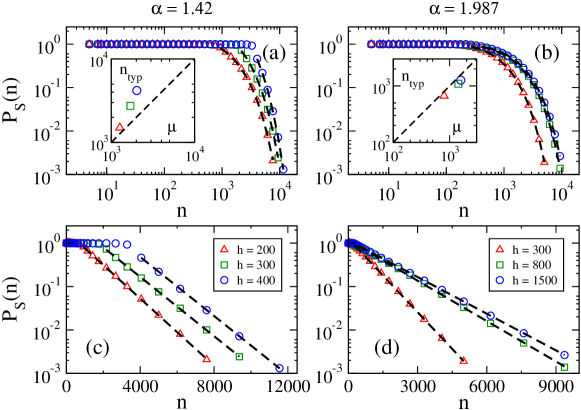
Figure 6: Survival probability $P_{\text{S}}(n)$ as a function of $n$ (symbols) for the RL-fSM with $K=6.908745$ and some combinations of $\alpha$ and $h$: (a,c) $\alpha=1.42$ and (b,d) $\alpha=1.987$; $h$ grows from left to right, as labeled in the figure. Upper and lower panels contain the same curves, however the horizontal axes in the lower panels are in linear scale to better appreciate the exponential decay of $P_{\text{S}}(n)$. Dashed black lines are fittings of the data with Eq. (6). The $R^{2}-1$ values of the fittings are: (a,c) $1.2\times 10^{-4}$ ($h=200$), $1.4\times 10^{-4}$ ($h=300$), $4.4\times 10^{-6}$ ($h=400$), and (b,d) $1.9\times 10^{-5}$ ($h=300$), $1.5\times 10^{-4}$ ($h=800$), $5.1\times 10^{-6}$ ($h=1500$). Curves were computed from $M=10^{5}$ orbits. Insets in (a,b) show $n_{\text{typ}}$ vs. $\mu$. The values of $\mu$ were extracted by fitting Eq. (6) to the $P_{\text{S}}(n)$ curves in the main panels. The relation $n_{\text{typ}}=\mu$ (dashed lines) is shown as a reference.

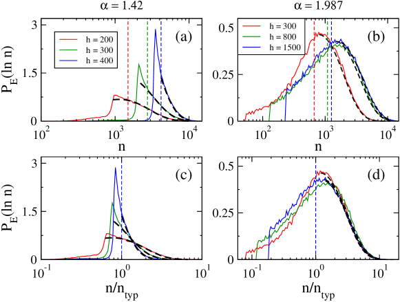
Figure 7: (a,b) Histograms for the frequency of escape $P_{\text{E}}(\ln n)$. Same color code as in Fig. 6. The typical escape times $n_{\text{typ}}=\exp\langle\ln n\rangle$ are indicated by the vertical dashed lines. Histograms were computed from $M=10^{5}$ orbits. Black dashed lines are Eq. (11). (c,d) $P_{\text{E}}(\ln n)$ as a function of $n/n_{\text{typ}}$; same histograms as in panels (a,b), respectively. (a,c) $\alpha=1.42$ and (b,d) $\alpha=1.987$.

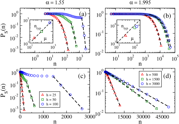
Figure 8: Survival probability $P_{\text{S}}(n)$ as a function of $n$ (symbols) for the RL-fSM with $K=7.5$ and some combinations of $\alpha$ and $h$: (a,c) $\alpha=1.55$ and (b,d) $\alpha=1.995$; $h$ grows from left to right, as labeled in the figure. Upper and lower panels contain the same curves, however the horizontal axes in the lower panels are in linear scale to better appreciate the exponential decay of $P_{\text{S}}(n)$. Dashed black lines are fittings of the data with Eq. (6). The $R^{2}-1$ values of the fittings are: (a,c) $2.1\times 10^{-5}$ ($h=25$), $4.2\times 10^{-4}$ ($h=50$), $1.1\times 10^{-3}$ ($h=100$), and (b,d) $1.6\times 10^{-5}$ ($h=500$), $6.5\times 10^{-5}$ ($h=1500$), $3.4\times 10^{-4}$ ($h=3000$). Curves were computed from $M=10^{5}$ orbits. Insets in (a,b) show $n_{\text{typ}}$ vs. $\mu$. The values of $\mu$ were extracted by fitting Eq. (6) to the $P_{\text{S}}(n)$ curves in the main panels. The relation $n_{\text{typ}}=\mu$ (dashed lines) is shown as a reference.

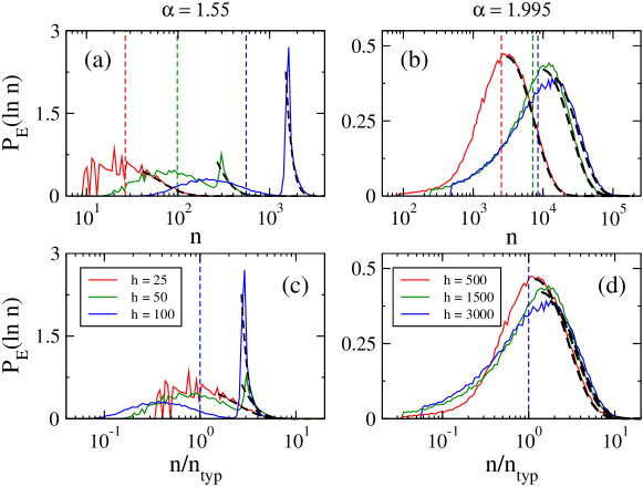
Figure 9: (a,b) Histograms for the frequency of escape $P_{\text{E}}(\ln n)$. Same color code as in Fig. 8. The typical escape times $n_{\text{typ}}=\exp\langle\ln n\rangle$ are indicated by the vertical dashed lines. Histograms were computed from $M=10^{5}$ orbits. Black dashed lines are Eq. (11). (c,d) $P_{\text{E}}(\ln n)$ as a function of $n/n_{\text{typ}}$; same histograms as in panels (a,b), respectively. (a,c) $\alpha=1.55$ and (b,d) $\alpha=1.995$.

Then, in Fig. 6, we present $P_{\text{S}}(n)$ as a function of $n$ for the RL-fSM with $K=6.908745$ and two values of $\alpha$ [(a,c) $\alpha=1.42$ and (b,d) $\alpha=1.987$] for some values of $h$. In Fig. 7(a,b), we plot the corresponding $P_{\text{E}}(\ln n)$ histograms.

For increasing $h$ both functions $P_{\text{S}}(n)$ and $P_{\text{E}}(\ln n)$ are displaced to the right as in the ergodic phase space case, see Figs. 2 and 3; this is expected since particles take longer to escape the higher the hole is. However, now $P_{\text{S}}(n)$ can not be described by a simple exponential decay, as in Eq. (6). We stress that not even the survival probability curves reported in Fig. 6(b), which look like simple exponentials, can be fitted by Eq. (6) in the complete range. This is not a big surprise since the exponential decay of $P_{\text{S}}(n)$ is only expected for strongly chaotic systems [20, 22, 23, 24], which is not the case with the values of $\alpha$ we chose in Figs. 6 and 7 [see Fig. 3(a,b)].

In Figs. 8 and 9, we present $P_{\text{S}}(n)$ and $P_{\text{E}}(\ln n)$, respectively, for the RL-fSM now with $K=7.5$ and (a,c) $\alpha=1.55$ and (b,d) $\alpha=1.995$. Here we also observe, as expected since the phase space is not ergodic [see Fig. 3(c,d)], that $P_{\text{S}}(n)$ and $P_{\text{E}}(\ln n)$ strongly depend on the map parameters.

Nevertheless we found that the decay of $P_{\text{S}}(n)$ in both cases, Figs. 6 and 8, is indeed exponential for large times. See the black dashed lines in those figures which are fittings of the $P_{\text{S}}(n)$ curves with Eq. (6). In the captions of Figs. 6 and 8, we report the $R^{2}$ (coefficient of determination) values of the fittings which validate the exponential decay of $P_{\text{S}}(n)$; in fact, the values of $R^{2}$ are so close to one that we better report $R^{2}-1$. Clearly, even when the tail of $P_{\text{S}}(n)$ can be fitted with Eq. (6), the values of $\mu$ extracted from the fittings can not always be identified with $n_{\text{typ}}$ as displayed in the insets of Figs. 6(a,b) and 8(a,b). Luckily, once we know that the tail of $P_{\text{S}}(n)$ in Figs. 6 and 8 is well described by Eq. (6), by the use of Eq. (8) we can estimate the tail of $P_{\text{E}}(\ln n)$ as

$$P_{\text{E}}(\ln n)\sim\frac{n}{\mu}\exp\left(-\frac{n}{\mu}\right).$$ (11)

Indeed, Eq. (11) describes well the tail of $P_{\text{E}}(\ln n)$ for all the parameter combinations reported in Figs. 7(a,b) and 9(a,b), see the dashed lines.

Finally, it is pertinent to mention that even when we were able to describe the tails of $P_{\text{S}}(n)$ and $P_{\text{E}}(\ln n)$ with Eqs. (6) and (11), respectively, these scattering functions can not be scaled neither with $n_{\text{typ}}$ nor with $\mu$. See for example the histograms of $P_{\text{E}}(\ln n)$ as a function of $n/n_{\text{typ}}$ in Figs. 7(c,d) and 9(c,d).

4 Discussion and conclusions

In this work, we characterized the leaking of orbits from the phase space of the Riemann-Liouville fractional standard map (RL-fSM). The RL-fSM is parameterized by $K$ and $\alpha\in(1,2]$ which control the strength of nonlinearity and the fractional order of the derivative of the corresponding fractional kicked rotor. It is important to stress that, to the best of our knowledge, the scattering properties of maps with memory have not been explored before.

We computed the frequency of escape $P_{\text{E}}(n)$ and the survival probability $P_{\text{S}}(n)$, more specifically $P_{\text{S}}(\ln n)$, for a hole of hight $h$ placed in the action axis. We explored two scenarios: one where the phase space of the RL-fSM is ergodic, see e.g. Figs. 1 and 2, and another where the phase space is non-ergodic, see e.g. Fig. 3.

When the phase space of the RL-fSM is ergodic we found that $P_{\text{E}}(n)$ and $P_{\text{S}}(\ln n)$ are both scale invariant with the typical escape time $n_{\text{typ}}=\exp\langle\ln n\rangle$, so they are well described by universal curves; see Fig. 4. This is in agreement with previous studies on leaking form discontinuous maps and dissipative maps [22, 23]. Moreover, for strongly chaotic systems, it has been shown that the survival probability can be obtained from the solution of the diffusion equation describing the transport of particles along the phase space as [21, 22]

$$P_{\text{S}}(n)\approx\exp\left(-\frac{\pi^{2}D}{4h^{2}}n\right),$$ (12)

where $D$ is the diffusion coefficient. Therefore, by equating Eqs. (9) and (12) and with the help of Eq. (10), we can infer the diffusion coefficient of the RL-fSM as

$$D\approx\frac{4}{\pi^{2}}\frac{h^{2}}{n_{\text{typ}}}\propto K^{2}.$$ (13)

It is relevant to highlight the independence of $D$ on $\alpha$.

When the phase space of the RL-fSM is not ergodic, even though we were able to characterize the tails of $P_{\text{E}}(n)$ and $P_{\text{S}}(\ln n)$ by means of Eqs. (6) and (11), respectively, both scattering functions showed clear non-universal and parameter-dependent behavior, see e.g. Figs. 6 to 9. That is, neither $P_{\text{E}}(n)$ nor $P_{\text{S}}(\ln n)$ can be scaled.

It is important to stress that for the RL-fSM we observe the exponential decay of $P_{\text{S}}(n)$ even when the phase space is not ergodic (for sufficiently large iteration times), see Figs. 6 and 8. This should be contrasted with other maps characterized by a non-ergodic phase space: for example, due to stickiness, $P_{\text{S}}(n)$ is known to develop asymptotic power-law tails in the case of mixed-chaotic dynamics [24, 25] and, due to Fermi acceleration, the decay of $P_{\text{S}}(n)$ as a stretched exponential was reported in [26].

We hope that our results may motivate further numerical as well as theoretical studies on the scattering properties of fractional dynamical systems in the context of General Fractional Dynamics (GFDynamics), recently established by Tarasov in [18].

Appendix A

To avoid the saturation of the main text, here we present the Poincaré surfaces of section for the RL-fSM with the parameters used to compute the survival probability $P_{\text{S}}(n)$ and the frequency of escape $P_{\text{E}}(\ln n)$ of Figs. 2-LABEL:Fig07.

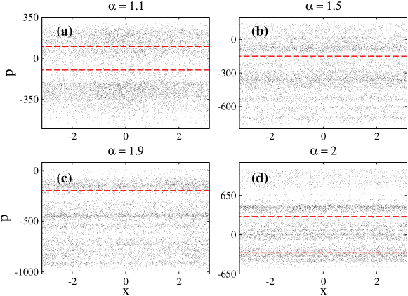
Figure 1: Poincaré surfaces of section for the RL-fSM with $K=6.908745$ for the values of $\alpha$ used to compute $P_{\text{S}}(n)$ and $P_{\text{E}}(\ln n)$ of Fig. 2. A single initial condition with $x_{0}=0$ and a random $p_{0}\in(0,2\pi/100)$ was iterated $10^{4}$ times. Holes in the action axis are located at $p=\pm h$ (red dashed lines) with (a) $h=100$, (b) $h=150$, (c) $h=200$, and (d) $h=300$.

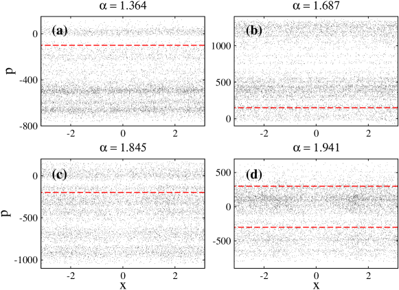
Figure 2: Poincaré surfaces of section for the RL-fSM with $K=7.5$ for the values of $\alpha$ used to compute $P_{\text{S}}(n)$ and $P_{\text{E}}(\ln n)$ of Fig. 3. A single initial condition with $x_{0}=0$ and a random $p_{0}\in(0,2\pi/100)$ was iterated $10^{4}$ times. Holes in the action axis are located at $p=\pm h$ (red dashed lines) with (a) $h=100$, (b) $h=150$, (c) $h=200$, and (d) $h=300$.

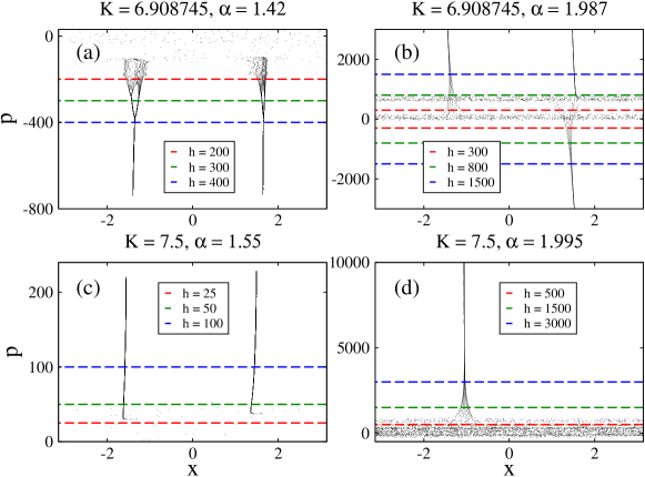
Figure 3: Poincaré surfaces of section for the RL-fSM with (a,b) $K=6.908745$ and (c,d) $K=7.5$ for the values of $\alpha$ used to compute $P_{\text{S}}(n)$ and $P_{\text{E}}(\ln n)$ of Figs. LABEL:Fig06 and LABEL:Fig07. A single initial condition with $x_{0}=0$ and a random $p_{0}\in(0,2\pi/100)$ was iterated $10^{4}$ times. Dashed lines indicate the position of holes in the action axis at $p=\pm h$.

References

- [1] E. Ott, Chaos in dynamical systems (Cambridge Univ. Press, 2008).
- [2] B. V. Chirikov, Research concerning the theory of nonlinear resonance and stochasticity, Preprint 267, Institute of Nuclear Physics, Novosibirsk (1969). Engl. Trans., CERN Trans. (1971) 71-40.
- [3] G. M. Zaslavsky, The simplest case of a strange attractor, Phys. Lett. A 69 (1978) 145–147.
- [4] F. Borgonovi, Localization in discontinuous quantum systems, Phys. Rev. Lett. 80 (1998) 4653.
- [5] V. E. Tarasov and G. M. Zaslavsky, Fractional equations of kicked systems and discrete maps, J. Phys. A 41 (2008) 435101.
- [6] M. Edelman and V. E. Tarasov, Fractional standard map, Phys. Lett. A 374 (2009) 279–285.
- [7] V. E. Tarasov, Fractional dynamics and discrete maps with memory, in Fractional Dynamics: Applications of Fractional Calculus To Dynamics Of Particles, Fields And Media, Book Series in Nonlinear Physical Science, Springer, Berlin (2011) 409–453.
- [8] V. E. Tarasov, Integral equations of non-integer orders and discrete maps with memory, Mathematics 9 (2021) 1177.
- [9] V. E. Tarasov, Fractional dynamics with non-local scaling, Commun. Nonlinear Sci. Numer. Simulat. 102 (2021) 105947.
- [10] M. Edelman and L. A. Taieb, New types of solutions of non-linear fractional differential equations, in Advances in Harmonic Analysis and Operator Theory; Series: Operator Theory: Advances and Applications, A. Almeida, L. Castro, F.-O. Speck (Eds.) (Springer, Basel, 2013), pp. 139–155.
- [11] M. Edelman, Dynamics of nonlinear systems with power-law memory, in Volume 4 Applications in Physics, Part A, Handbook of fractional calculus with applications, V. E. Tarasov (Ed.) (De Gruyter, Berlin, Boston, 2019) pp. 103–132.
- [12] M. Edelman, Fractional standard map: Riemann-Liouville vs. Caputo, Commun. Nonlinear. Sci. numer. Simulat. 16 (2011) 4573–4580.
- [13] M. Edelman, Universal fractional map and cascade of bifurcations type attractors, Chaos 23 (2013) 033127.
- [14] V. E. Tarasov, and M. Edelman, Fractional dissipative standard map, Chaos 20 (2010) 023127.
- [15] V. E. Tarasov, Fractional Zaslavsky and Henon discrete maps, Chapter 1 in Long-range Interaction, Stochasticity and Fractional Dynamics, A. C. J. Luo and V. Afraimovich (Eds.), Springer, HEP (2010) 1–26.
- [16] V. E. Tarasov, Review of some promising fractional physical models, Int. J. Modern Phys. B 27 (2013) 1330005.
- [17] M. Edelman, Caputo standard -family of maps: Fractional difference vs. fractional, Chaos 24 (2014) 023137.
- [18] V. E. Tarasov, General fractional dynamics, Mathematics 9 (2021) 1464.
- [19] M. Edelman and A. B. Helman, Asymptotic cycles in fractional maps of arbitrary positive orders, Fract. Calc. Appl. Anal. 25 (2022) 181–206.
- [20] E. G. Altmann, J. S. E. Portela, and T. Tél, Leaking chaotic systems, Rev. Mod. Phys. 85 (2013) 869.
- [21] J. A. deOliveira, C. P. Dettmann, D. R. daCosta, and E. D. Leonel, Scaling invariance of the diffusion coefficient in a family of two-dimensional Hamiltonian mappings, Phys. Rev. E 87 (2013) 062904.
- [22] J. A. Méndez-Bermúdez, A. J. Martínez-Mendoza, A. L. P. Livorati, and E. D Leonel, Leaking of trajectories from the phase space of discontinuous dynamics, J. Phys. A: Math. Theor. 48 (2015) 405101
- [23] J. A. de Oliveira, R. M. Perre, J. A. Méndez-Bermúdez, and E. D. Leonel, Leaking of orbits from the phase space of the dissipative discontinuous standard mapping, Phys. Rev. E 103 (2021) 012211.
- [24] T. Srokowski, J. Okolowicz, S. Drozdz, and A. Budzanowski, Fusion cross section from chaotic scattering, Phys. Rev. Lett. 71 (1993) 2867.
- [25] A. L. P. Livorati, T. Kroetz, C. P. Dettmann, I. L. Caldas, and E. D. Leonel, Stickiness in a bouncer model: A slowing mechanism for Fermi acceleration, Phys. Rev. E 86 (2012) 036203.
- [26] C. P. Dettmann, and E. D. Leonel, Escape and transport for an open bouncer: Stretched exponential decays, Physica D 241 (2012) 403.