Smooth digital terrain modelling in irregular domain using adaptive finite element thin plate spline smoother

Abstract

Digital terrain models of geological information occasionally require smooth data in domains with complex irregular boundaries due to its data distribution. Traditional thin plate splines produce visually pleasing surfaces, but they are too computationally expensive for data of large sizes. Finite element thin plate spline smoother (TPSFEM) is an alternative that uses first-order finite elements to efficiently interpolate and smooth large data sets. Previous studies focused on regular square domains, which are insufficient for real-world applications. This article builds on prior work and investigates the performance of the TPSFEM and adaptive mesh refinement for real-world data sets in irregular domains. The Dirichlet boundaries are approximated using the thin plate spline and data-dependent weights are applied to prevent over-refinement near boundaries. Three geological surveys (aerial, terrestrial and bathymetric) with distinct data distribution patterns were tested in the numerical experiments. We found that irregular domains with adaptive mesh refinement significantly improve the efficiency of the interpolation. While the inconsistency in approximated boundary conditions, we may prevent it using additional constraints like weights. This finding is also applicable to other finite element-based smoothers.

1 Introduction

Digital terrain models (DTMs) represent continuous terrain surfaces constructed using geological surveys and have been widely applied in various areas including mining engineering (Wang et al. 2018), climate science (Hutchinson 1995) and geological modelling (Hillier et al. 2014). It is also referred to as a digital elevation model or digital height model and their distinctions were discussed in (Li et al. 2004). Geological surveys include aerial, terrestrial and bathymetric surveys, depending on the application and terrain (Li et al. 2004). In recent years, unmanned vehicles such as small-scale unmanned aerial vehicles have been widely applied in both civil and military applications. Noise is often present in sampled data and the DTMs often require smoothers like the thin-plate spline (TPS) to extract underlying patterns and produce smooth surfaces. While the TPS is flexible and adapted to varied data distributions, its computational costs and memory requirements are impractical for large data sets. Many techniques were developed to improve its efficiency, including compactly supported radial basis functions and fast multipole methods discussed in Chapter 2 of (Fang 2021). They addressed the computational issue in different ways but their limitations weaken the practicability in real-world applications.

The finite element thin plate spline smoother (TPSFEM) was developed by Roberts et al. (2003) to interpolate and smooth large data sets. Finite element-based smoothers have been studied by other authors including Hutchinson (1995), Ramsay (2002) and Chen et al. (2018) and most of them use second or higher-order finite elements. The TPSFEM is the first to use first-order finite elements to obtain a sparser system of equations and achieves higher efficiency. It was designed for surface fitting and data mining applications and the performance has been verified for both 2D and 3D spaces (Stals and Roberts 2006). Adaptive mesh refinement and error indicators of the TPSFEM were investigated, which further enhance its efficiency (Fang and Stals 2022).

Previous studies on the TPSFEM and adaptive mesh refinement focused on regular square domains and this is insufficient for real-world applications. The observed data are scaled and fitted inside at the centre and far away from boundaries, which allows a smooth transition from interpolants to approximated boundary conditions (Stals and Roberts 2006). This leads to a potentially large number of nodes lying in regions without data and the efficiency deteriorates. This phenomenon is more significant for irregularly distributed data from applications such as geospatial modelling. A domain with complex irregular shapes may fit the data more closely and resolve this issue, but it also faces several challenges. For instance, it requires more accurate approximated boundary conditions since a smaller distance between the data and boundaries may affect the accuracy of resulting interpolants.

In this article, we examine the performance of the TPSFEM and adaptive refinement for the DTM on irregular domains. We build irregular domains that fit the diverse distribution patterns from the geological survey data. We also approximate Dirichlet boundary conditions of the TPSFEM using the TPS with a small subset of sampled data. Moreover, data-dependent weights are applied to the error indicators to avoid over-refinement near boundaries shown in the previous research. Numerical experiments were conducted using three real-world geological surveys to evaluate the performance under different distribution patterns caused by the survey strategies. While we investigate in the scope of the TPSFEM, the idea may apply to other finite element-based interpolation techniques.

The remainder of this article is organised as follows. The formulation and adaptive refinement of the TPSFEM are provided in Section 2. The construction of polygonal domains is shown in Section 3. The Dirichlet boundary conditions approximated using the TPS are discussed in Section 4. Data-dependent weights for the error indicators are explained in Section 5. The three geological surveys investigated in the experiments are shown in Section 6. Numerical experiments, results and discussions are presented in Section 7. Conclusions of findings are summarised in Section 8.

2 Finite element thin plate spline smoother

A short description of the TPSFEM is provided in this section and a detailed one was given by Stals and Roberts (2006). Given data $\{(\bm{x}_{i},y_{i}):i=1,2,\ldots,n\}$ of size $n$, where $\bm{x}_{i}\in\mathbb{R}^{d}$ and $y_{i}\in\mathbb{R}$ are $i$th $d$-dimensional predictor value and response value, respectively. The TPSFEM $s(\bm{x})=\bm{b}(\bm{x})^{T}\bm{c}$ is represented as a combination of $m$ piecewise linear basis functions $\bm{b}$, where $\bm{b}=[b_{1},\ldots,b_{m}]^{T}$ and $\bm{c}$ are corresponding coefficients. Auxiliary functions $\bm{u}=[\bm{u}_{1},\ldots,\bm{u}_{d}]^{T}$ were introduced to approximate the gradient of $s$, where $\bm{u}_{k}$ approximate the gradient of $s$ in dimension $k$ for $1\leq k\leq d$, $\bm{u}_{k}(\bm{x})=\bm{b}(\bm{x})^{T}\bm{g}_{k}$ and $\bm{g}_{k}$ are corresponding coefficients (Roberts et al. 2003).

The TPSFEM $s$ minimises

$$J(\bm{c},\bm{g}_{1},\ldots,\bm{g}_{d})=\bm{c}^{T}A\bm{c}-2\bm{d}^{T}\bm{c}+\bm{y}^{T}\bm{y}/n+\alpha\sum_{k=1}^{d}\bm{g_{k}}^{T}L\bm{g_{k}},$$ (1)

subject to constraint $L\bm{c}=\sum_{k=1}^{d}G_{k}\bm{g}_{k}$, where $\bm{d}=\frac{1}{n}\sum_{i=1}^{n}\bm{b}(\bm{x}_{i})y_{i}$, $\bm{y}=[y_{1},\ldots,y_{n}]^{T}$, $A=\frac{1}{n}\sum_{i=1}^{n}\bm{b}(\bm{x}_{i})\bm{b}(\bm{x}_{i})^{T}$, $L$ is a discrete approximation to the negative Laplacian and $G_{k}$ is a discrete approximation to the gradient operator in dimension $k$ for $1\leq k\leq d$. Matrix $A$ and vector $\bm{d}$ are constructed by a single scan of the data and project information of data onto the finite element mesh. Smoothing parameter $\alpha$ balances the goodness of fit and smoothness of $s$ and it is calculated using the generalised cross-validation (Fang 2021). We rewrite Equation (1) and the constraint as the solution of a system of linear equations using Lagrange multipliers.

For example, the system in a two-dimensional domain with Dirichlet boundary conditions is written as

$$\begin{bmatrix}A&\bm{0}&\bm{0}&L\\ \bm{0}&\alpha L&\bm{0}&-G_{1}^{T}\\ \bm{0}&\bm{0}&\alpha L&-G_{2}^{T}\\ L&-G_{1}&-G_{2}&\bm{0}\end{bmatrix}\begin{bmatrix}\bm{c}\\ \bm{g}_{1}\\ \bm{g}_{2}\\ \bm{w}\end{bmatrix}=\begin{bmatrix}\bm{d}\\ \bm{0}\\ \bm{0}\\ \bm{0}\end{bmatrix}-\begin{bmatrix}\bm{h}_{1}\\ \bm{h}_{2}\\ \bm{h}_{3}\\ \bm{h}_{4}\end{bmatrix},$$ (2)

where $\bm{w}$ is a Lagrange multiplier and Dirichlet boundary information is stored in $\bm{h}_{1}$, $\bm{h}_{2}$, $\bm{h}_{3}$, $\bm{h}_{4}$. The system’s dimension is independent of the number of data points $n$, which is more efficient for large data sets. The boundary information of the TPSFEM is incorporated in the system as described on page 187 of (Stals and Roberts 2006). In this article, we only consider the Dirichelt boundary conditions, which are more stable for adaptive refinement (Fang 2021).

Suppose that the finite element spaces satisfy Assumptions 1 to 5 listed on pages 212 to 214 of (Roberts et al. 2003), then there exist constants $C_{1}>1$ and $\alpha_{0}>0$ such that for all smooth function $f\in H^{2}(\Omega)$, which models response values $\bm{y}$, the expected errors of the TPSFEM satisfy

$$E||s(\bm{y})-f||_{L^{2}(\Omega)}^{2}\preceq\left(\alpha+h^{4}+d_{X}^{4}\right)||f||_{H^{2}(\Omega)}^{2}+\frac{\sigma^{2}}{\alpha^{1/2}}\frac{(h^{4}+d_{X}^{4})}{h^{2}},$$ (3)

$$E|s(\bm{y})-f|_{H^{1}(\Omega)}^{2}\preceq\frac{1}{\alpha^{1/2}}\left(\alpha+h^{4}+d_{X}^{4}\right)||f||_{H^{2}(\Omega)}^{2}+\frac{\sigma^{2}}{\alpha}\frac{(h^{4}+d_{X}^{4})}{h^{2}},$$ (4)

provided that $h$ and $\alpha$ satisfy $h>C_{1}d_{X}$ and $d_{X}^{4}+h^{4}<\alpha<\alpha_{0}$. The $L^{2}(\Omega)$ norm and Sobolev semi-inner-products $H^{1}(\Omega)$ and $H^{2}(\Omega)$ are defined on page 209 of (Roberts et al. 2003) and $\sigma^{2}$ is the variance of measurement errors.

2.1 Adaptive refinement

The accuracy of the TPSFEM is improved by adaptive refinement that iteratively refines a subset of elements marked by an error indicator. Four error indicators were adapted and tested for the TPSFEM and the resulting adaptively refined meshes achieve the target accuracy with fewer nodes and higher efficiency compared to uniform meshes (Fang 2021). These four error indicators are the auxiliary problem, recovery-based, norm-based and residual-based error indicators. Their detailed descriptions are provided on pages 46, 51, 53 and 56 of (Fang 2021), respectively. The auxiliary problem and residual-based error indicators use local data points to build locally more accurate approximations or estimate residuals directly. The recovery-based error indicator and norm-based error indicators process the gradients or second-order derivatives to indicate large errors. They do not access local data directly and only use interpolant $s$ and finite element mesh. In the numerical experiments, we choose the auxiliary problem and recovery-based error indicators, which are representative out of the four error indicators.

The auxiliary problem error indicator indicates errors by building a locally more accurate approximation and comparing it with interpolant $s$ (Mitchell 1989). The local approximations are obtained by building the TPSFEM on a small subset of the domain using a cluster of neighbouring data points. The error norm is then calculated using the difference between local approximations and interpolant $s$. The accuracy of auxiliary problems depends on several factors, including the smoothing parameter $\alpha$, mesh size $h$, size and distribution of data points and boundary condition. The error indicator value $\eta_{\tau}$ of a triangle $\tau$ is defined as

$$\eta_{\tau}^{2}=\int_{\tau}\left[\sum_{i=1}^{d}\left(\frac{\partial}{\partial x_{i}}(s-\widehat{s})\right)^{2}\right]\,d\bm{x},$$

where $s$ is the TPSFEM interpolant over $\Omega$ and $\widehat{s}$ is the local approximation.

The recovery-based error indicator estimates the error by post-processing discontinuous gradients of $s$ across inter-element boundaries (Zienkiewicz and Zhu 1987). The TPSFEM is represented by piecewise linear basis functions with zero-order continuity and current gradient approximations $D^{1}s$ are piecewise constants. We post-process $s$ to improve the gradient approximation and the error is estimated as the energy norm of the difference between the current and improved gradient approximations $\widehat{D}^{1}s$. The recovery-based error indicator only uses information on the mesh, which is more computationally efficient compared to the auxiliary problem error indicator. Its error indicator value $\eta_{\tau}$ is set as

$$\eta_{\tau}^{2}=\int_{\tau}(\widehat{D}^{1}s-D^{1}s)^{2}\,d\bm{x}.$$

3 Irregular domain

Previous TPSFEM studies rescaled predictor values of the data and fit them inside regular square domains and far away from boundaries (Stals and Roberts 2006). The finite element meshes are then generated in the domain and used to build the TPSFEM. While this is applicable for data with varied distribution patterns, large spaces in domains may not contain any data points. For instance, if data is contained inside $[0.2,0.8]^{2}$ region of a square $[0,1]^{2}$ domain, at most $36\%$ of the domain may contain data points. Since the boundary information is unknown for data sets in many real-world applications, these regions allow a smooth transition from boundaries to interpolants. However, a large number of nodes are placed in regions without any data point and may not markedly contribute to improving the accuracy of interpolants. This may affect the efficiency of the TPSFEM especially when the data are irregularly distributed.

The data distribution patterns often vary across applications. For example, aerial surveys collect data through flights that form frames and are less affected by terrain (Caughley 1977). In contrast, bathymetric surveys are often limited by the bank of a water body. The latter often leads to data sets with complex external geometric shapes. We may use polygonal domains that fit the data closely to reduce the area of regions without any data points, which may improve the efficiency of finite element meshes.

We build a polygon domain by finding a set of vertices and edges to fit the exterior of the observed data. A polygonal mesh with triangular elements embedded in that domain is then generated automatically. The vertices of the polygonal domain are estimated using algorithms like alpha shape that generalise bounding polygons containing the data (Xu and Harada 2003). The shape of the domain depends on an alpha parameter that controls the tightness of the fitting bounding box and is defined by vertices and edges instead of arcs. These two functionalities are achieved using Python libraries alphashape and pygmsh. An example finite element mesh is illustrated in Figure 1(a).

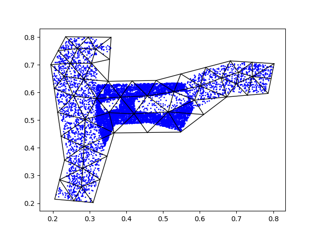
(a)

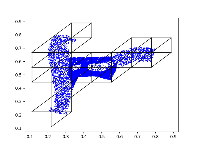
(b)

Figure 1: Meshes generated by (a) building a polygonal domain; and (b) trimming elements without data. The data points are represented as blue dots.

An alternative is to build a square domain and remove elements that do not contain any data points. This process is described in Algorithm 1 and begins with a mesh generated within a square domain covering the data. We iterate through elements near boundaries and remove ones without any data points. An example finite element mesh is shown in Figure 1(b). We refer to the first approach as the polygon approach and the second one as the trim approach in the rest of the article.

Algorithm 1 Meshing by trimming elements without data

1:build a triangular mesh in a square domain that covers the observed data

2:while not all boundary edges are marked do

3:     for each boundary edge do

4:         find triangle this boundary edge lies on

5:         calculate the number of data points covered by the triangle

6:         if number of data points is zero then

7:              remove this boundary edge

8:              set two other edges of the triangle as boundary edges

9:         else

10:              mark this boundary edge as trimmed

11:         end if

12:     end for

13:end while

14:set geometric information

Both approaches generate triangular meshes in irregular domains with distinct strengths and limitations. The polygon approach constructs a bounding polygonal domain from data directly, which adapts to random data distributions and controls the distance from the data to boundaries illustrated in Figure 1(a). However, it requires parameter tuning, including alpha parameter and mesh sizes, and may not perform well when the data distributes in a concave polygon. In contrast, the trim approach is robust and only requires the mesh size of the initial mesh, which decides the efficiency and distance from the data to boundaries. It often leads to inconsistent distance from the data to boundaries, as shown in Figure 1(b). It may also generate meshes with disconnected elements and the initial mesh size should be estimated by the largest distance between nearby data points.

One major difference between these two approaches is the varied mesh sizes and shapes of elements. The trim approach produces meshes with regular elements as the process does not alter their sizes and shapes. In contrast, the alphashape approach often leads to elements with different sizes and shapes, as illustrated in Figure 1(a). Consequently, bounds on angles of triangular elements may no longer be optimal. Meshes in the square domain consist of only isosceles right triangular elements with $45^{\circ}$ or $90^{\circ}$ angles. Using the newest node bisection, the resulting refined meshes will only contain isosceles right triangles. However, meshes produced by the alphashape approach may lead to more acute triangular elements after adaptive refinement. If angles in initial meshes are set between $[\theta_{min},\theta_{max}]$, angles of adaptive meshes will be bounded between $[\frac{1}{2}\theta_{min},2\theta_{max}]$ (Mitchell 1989). While this will not lead to long and thin triangles and deterioration of interpolation errors, it may affect the performance of adaptive refinement and error indicators. In this article, we focus on the alphashape approach and the results are shown in Section 7.

4 Boundary conditions

Boundary conditions have a large impact on the accuracy of the TPSFEM and adaptive refinement (Fang 2021). When the data is generated using a known model problem function, $\bm{c}$, $\bm{g}_{1},\ldots,\bm{g}_{d}$ and $\bm{w}$ values in Equation (2) are defined using the function and its derivatives, which helps to analyse the TPSFEM’s behaviour near boundaries (Stals and Roberts 2006). However, sampled data from real-world applications often do not contain boundary information and we used an average of response values to set $\bm{c}$ values for Dirichlet boundary conditions or use zero Neumann boundaries. Moreover, data points are placed far away from boundaries for a smooth transition.

When data is close to boundaries and approximated boundary conditions are not sufficiently accurate, a smooth transition between boundaries and interpolant $s$ may not be plausible and nearby surfaces become oscillatory. It may also mislead the error indicators such as the auxiliary problem error indicator and weaken the efficiency of resulting adaptively refined meshes (Fang and Stals 2022). Polygonal domains increase the proportion of elements that cover data, but they also reduce the distance from data to boundaries. Consequently, surfaces near boundaries may become oscillatory and adaptive refinement is often misdirected. This problem may be avoided using more accurate boundary conditions. We propose to build the traditional TPS introduced by Duchon (1977) using a subset of the data to approximate $\bm{c}$, $\bm{g}_{1},\ldots,\bm{g}_{d}$ and $\bm{w}$ values for Dirichlet boundary conditions.

The TPS is chosen for its favourable smoothing properties and compatibility with the TPSFEM. The TPS is flexible and efficient for small data sets (e.g. hundreds of data points). While the TPS’s interpolant also become unstable near boundaries, it can still greatly improve current boundary condition approximations (Fornberg et al. 2002). Roberts et al. (2003) argued that the TPSFEM has similar smoothing properties as the TPS except near boundaries where data is sparse. Using the TPS for boundary information allows us to combine the advantages of the TPSFEM and TPS. We use kernels of the TPS and its derivatives listed in Table 1 to approximate $\bm{c}$and $\bm{g}$ values, respectively. Variable $\bm{x}_{i,k}$ represents the $k$-th entry of $i$-th predictor value.

Table 1: Two-dimensional kernels for derivative approximations

Value	Kernel
$\bm{c}$	$r^{2}\log(r)$
$\bm{g}_{1}$	$(2\log{r}+1)(\bm{x}_{i,1}-\bm{x}_{j,1})$
$\bm{g}_{2}$	$(2\log{r}+1)(\bm{x}_{i,2}-\bm{x}_{j,2})$
$\bm{w}$	$\log{r}+4$

The performance of this approach is dependent on a set of factors, including the choice of kernel, number and choice of sampled data. Both the accuracy and computational costs of the TPS increase as the number of sampled data $n_{b}$ increases, for example, the construction of the TPS takes $O(n_{b}^{2})$ computation. Additionally, one evaluation of the TPS interpolant takes $O(n_{b})$ computation from each boundary information enquiry, which is significantly more expensive compared to calculating a given function for the PDEs. Therefore, the number of data points in the subset should be chosen considering both efficiency and accuracy. Moreover, since only a small subset of the data is chosen to build the TPS, the resulting interpolant will be heavily dependent on the sampling strategy. Currently, we choose them randomly to obtain a more stable global approximation. An alternative is concentrating on data points near boundaries to improve the accuracy, but it may also lose impacts from other regions.

5 Weighted error indicators

The two error indicators introduced in Section 2.1 were adapted to use data and they significantly improve the efficiency of the TPSFEM when the data are placed far away from boundaries. Though the performance may be affected by Neumann boundaries that lead to unstable surfaces near boundaries. A similar phenomenon has been observed while using polygonal domains with data close to boundaries. The inconsistency may mislead the error indicators to over-refine near boundaries as shown in Figure 2(a), which reduces the efficiency of resulting adaptive meshes.

We further improve the stability of the error indicators by factoring in local data density while indicating errors to avoid over-refinement. The data density has been applied to choose sampling positions of knots for radial basis functions as higher density often suggests higher priority (Fang 2021). The error indicators of the TPSFEM mark a value for each triangle pair to indicate whether it should be refined. However, the current value is only based on approximated errors and the element’s size. We incorporate the data density by scaling the error indicator value with a weight $w$ as defined by

$$w=\sqrt{n_{t}+n_{min}},$$

where $n_{t}$ is the number of data points covered by the triangle pair and $n_{min}$ is a small nonnegative value that ensures $w$ is nonzero. This weight leads to more refinement on regions with more data points, but elements without data may still be refined as weights will never be zero. The square root limits the effects of the weights such that resulting adaptive meshes will not only be dependent on the data density shown in Figure 2(b).

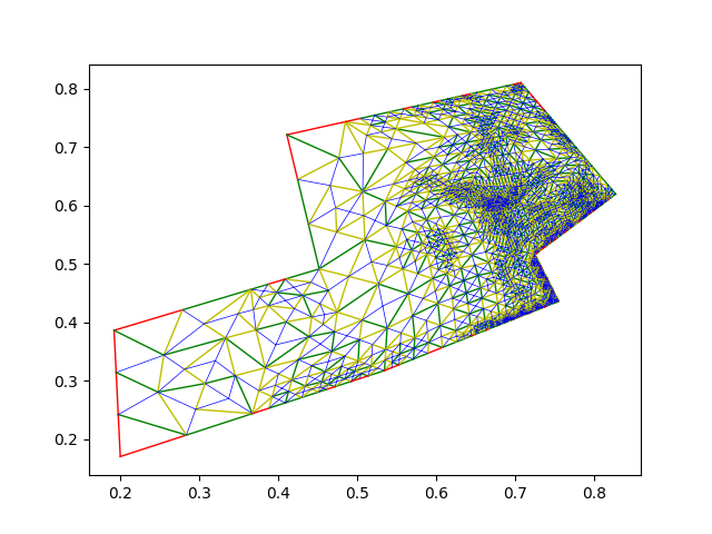
(a)

(b)

Figure 2: Adaptively refined meshes on the polygonal domain for River data with (a) over-refinement near boundaries; and (b) error indicators weighted using the number of data points.

An alternative is using entry values from matrix $A$ in Equation (2). Matrix $A$ is the data projection matrix and it contains information projected by predictor values $\bm{x}$ on the finite element meshes. If there is no data point inside the support of basis functions, its corresponding $A$ value will be zero. We find $A$ entry values that correspond to basis functions that cover the triangle pair and set the average as $w$. These $A$ are stored in the finite element mesh and are cheap to estimate. They also converge as the number of data points in the elements becomes extremely large, which prevents the effects of the data density from dominating the error indicator values. The weight based on the data size and $A$ values will be referred to as data weight and A weight, respectively.

6 Real-world Data

We evaluated the performance of the TPSFEM on polygonal domains using data sets from three geological surveys of the United States Geological Survey .

The first data set is airborne magnetic survey data collected from the Iron Mountain Menominee region of Michigan and Wisconsin (Drenth 2020). Precambrian rocks in the region are poorly mapped and the detailed high-resolution airborne magnetic survey is used to better understand its lithology and structure. It comprises 1,011,468 data points and variables including latitude, longitude and total magnetic field were selected for this study. The variations of magnetisation are related to differences in rock types.

The second data set contains ground observations collected by terrestrial laser scanner surveys in Grapevine Canyon near Scotty’s Castle, Death Valley National Park (Morris et al. 2020). It updated flood-inundation maps that were affected by a large flood in 2015 to current conditions. The observed data has been filtered of extraneous data such as vegetation, fences, power lines, and atmospheric interference for a continuous DTM. The resulting 122,104 data points, including latitude, longitude and elevation, were used to produce a digital terrain model of the area.

The third data set contains a nearshore bathymetric survey sampled at the mouth of the Unalakleet River in Alaska (Snyder et al. 2019). The survey comprises 895,748 data points consisting of latitude, longitude and height in meters regarding the reference ellipsoid. The data records depths from the seafloor to the echosounder and was collected using a small boat equipped with a single-beam sonar system.

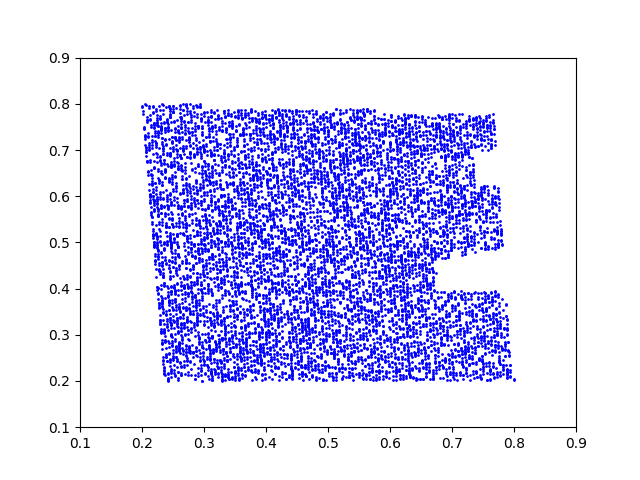
(a)

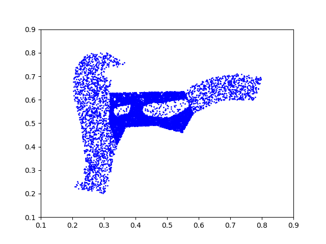
(b)

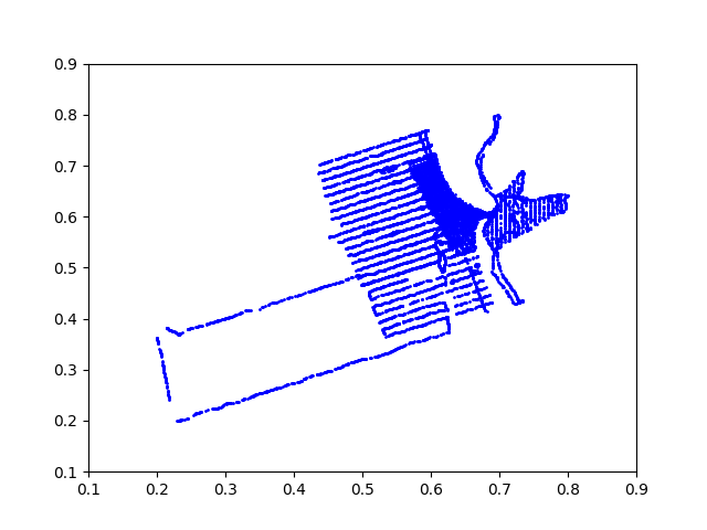
(c)

Figure 3: Distributions of a subset of randomly selected $\bm{x}$ variables in (a) Mountain; (b) Canyon and (c) River data sets.

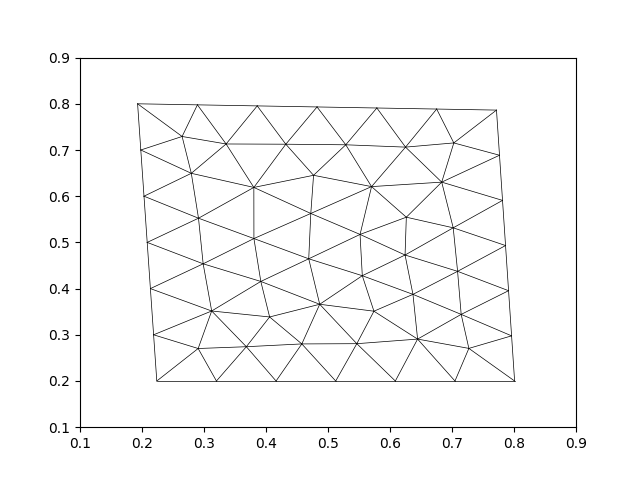
(a)

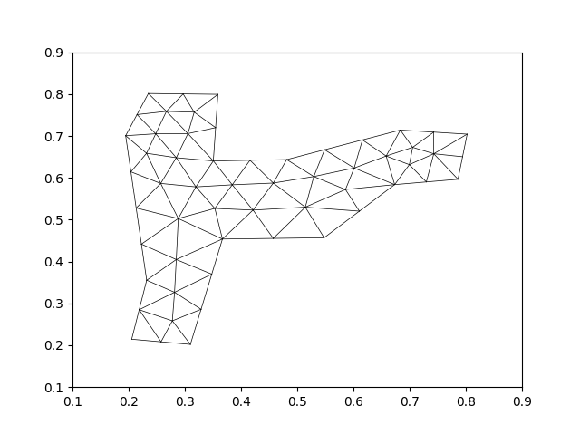
(b)

(c)

Figure 4: Finite element meshes for (a) Mountain; (b) Canyon and (c) River data sets.

These three data sets will be referred to as the Mountain data, Canyon data and River data in the rest of the article for clarity. They are chosen due to their distinct data distribution patterns as illustrated in Figure 3 and corresponding polygonal meshes are shown in Figure 4. The first data set was collected using an unmanned aerial vehicle and it collected data on transects, which were relatively uniform across the domain as shown in Figure 3(a). In contrast, the Canyon data in Figure 3(b) are limited by terrains and equipment. Sampled points of the ground observations concentrate on the bottom and steep sides of the deep canyon, which may be altered by the flood. Moreover, more observations are collected at the centre as illustrated by denser data points, which leads to uneven data densities. Similarly, the bathymetric survey in Figure 3(c) consists of routes of a boat that forms frames with different sparseness. More data points were sampled around the river mouth near point $[0.7,0.6]$ to model complex river beds. It also contains a subset of data points (e.g. routes in the bottom left), which are not the focus of this survey.

7 Numerical experiments

We conducted numerical experiments using geological data to evaluate the performance of the TPSFEM and adaptive refinement in square and polygonal domains. Results for polygonal domains generated using the alphashape approach are provided in Section 7.1 and ones generated using the trim approach are included in the supplementary materials. In square domains, we placed the data inside the $[0.2,0.8]^{2}$ region and set $[0,1]^{2}$ as the square domain. The predictor values $\bm{y}$ of the three data sets were sampled on different scales and we normalise them in the range of $[0,1]$ to allow easier comparison of their convergence rates. The performance of finite element meshes is measured using the root mean square error (RMSE) versus the number of nodes in meshes, where RMSE $=\big{(}\frac{1}{n}\sum_{i=1}^{n}\big{(}s(\bm{x}_{i})-y_{i}\big{)}^{2}\big{)}^{\frac{1}{2}}$.

7.1 Results

We evaluate the performance of the TPSFEM and adaptive refinement by examing their convergence plots and adaptively refined meshes. The convergence of RMSE versus the number of nodes in meshes for the Mountain, Canyon and River data sets are shown in Figures 7, 10 and 13, respectively. Each plot contains convergence rates of the TPSFEM using uniform refinement or adaptive refinement with the two error indicators and weights. Contour maps of resulting TPSFEM interpolants $s$ and adaptive meshes are also provided in Figures 6, 9 and 12 to illustrate the difference in performance.

7.1.1 Mountain Data

The Mountain data consists of relatively smooth surfaces and several oscillatory regions at the upper left corner of the domain, as shown in Figure 6(a). High peaks near point $[0.25,0.8]$ show high magnetic field readings and suggest potential mineral resources. Adaptive refinement of the TPSFEM successfully detects and iteratively refines these oscillatory regions to achieve the required accuracy as illustrated by the adaptive mesh in Figure 6(b). The mesh contains markedly finer elements over the peaks and coarse elements in other regions, which effectively reduces computational costs and memory requirements for building the TPSFEM.

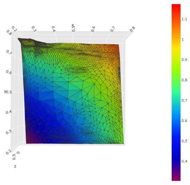
Figure 5: Surface triangulation plot of Mountain data on a polygonal domain.

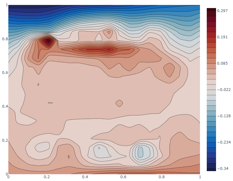
(a)

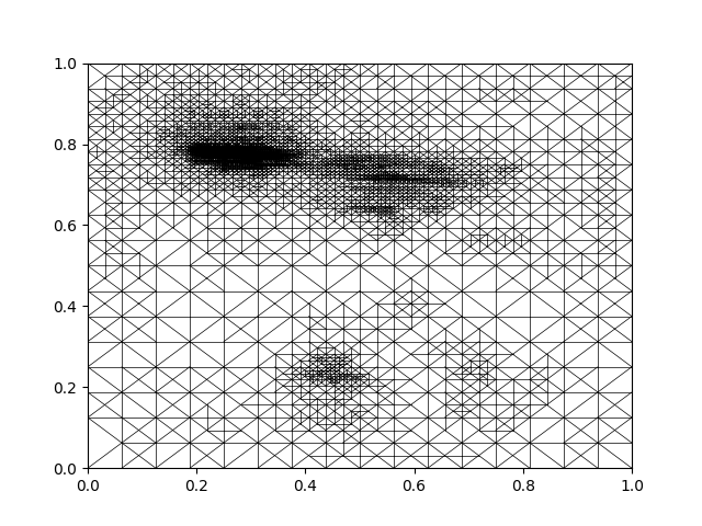
(b)

Figure 6: (a) Contour map; and (b) adaptive mesh of the Mountain data. (keep it for comparison only)

The convergence of the TPSFEM for the Mountain data is shown in Figure 7. Adaptive refinement outperforms uniform refinement for the Mountain data on both square and polygonal domains. Since the surfaces are smooth in most regions, the TPSFEM only require relatively coarse elements in those regions to achieve high accuracy, which is ideal for adaptive refinement. In Figure 7(a), the convergence of the RMSE on square domains using different weights varies markedly and the error indicators without weights achieve the highest convergence rates. Since the Mountain data only has relatively small oscillatory regions, error indicators without weights concentrate on refining those regions instead of other smooth surfaces. In contrast, the error indicator with A weights leads to more spread-out refinement due to the even data density and the convergence rates significantly lower than the others. While weights on the error indicators prevent over-refinement near boundaries, it may lead to negative impacts on adaptive refinement. Also, note that the auxiliary problem error indicator achieves higher convergence rates than the recovery-based error indicator as it is more sensitive to oscillation in small regions.

The shape of the Mountain data’s polygonal domain is close to a square domain as the transects of its aerial survey are not affected by the terrain as shown in Figure 3(a). Thus the major distinction between the two domains is the reduced distance from data to domain boundaries. Consequently, polygonal domains improve the efficiency of uniform meshes and adaptive meshes generated with A weights as shown in Figure 7(b). However, the RMSE of adaptive meshes generated without weights is slightly higher due to over-refinement near boundaries. The lowest RMSE achieved in Figure 7(b) is close to the one in Figure 7(a) but requires more nodes in meshes.

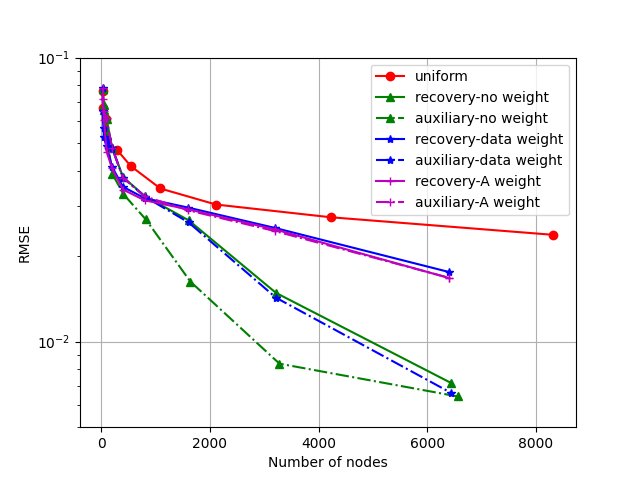
(a)

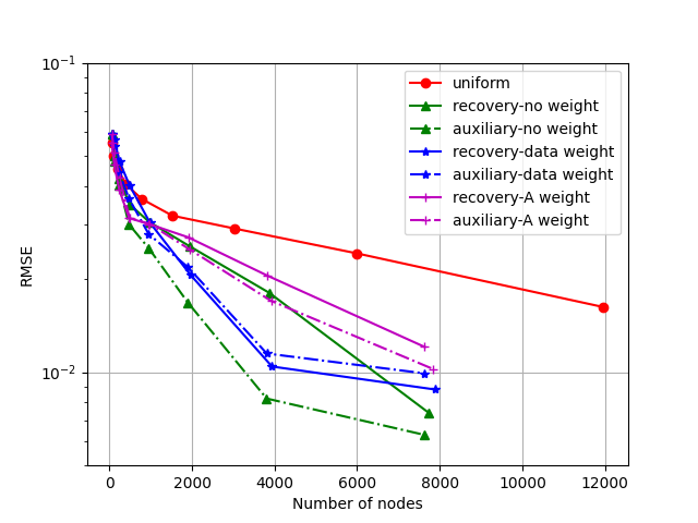
(b)

Figure 7: Convergence of RMSE for the Mountain data in (a) square domains; and (b) polygonal domains.

7.1.2 Canyon Data

The Canyon data consists of steep sides and gradual bottom of the observed canyon as shown in Figure 9(a). Since positions of sampling were determined by the terrain, the steep sides were near the exterior of the Canyon data. Those steep sides require finer elements to model and an example adaptive mesh is displayed in 9(b). In contrast, the bottom of the canyon and regions without data points achieve the required precision with only coarse elements.

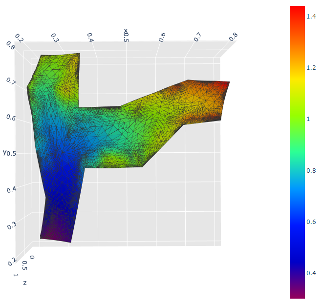
Figure 8: Surface triangulation plot of Canyon data on a polygonal domain.

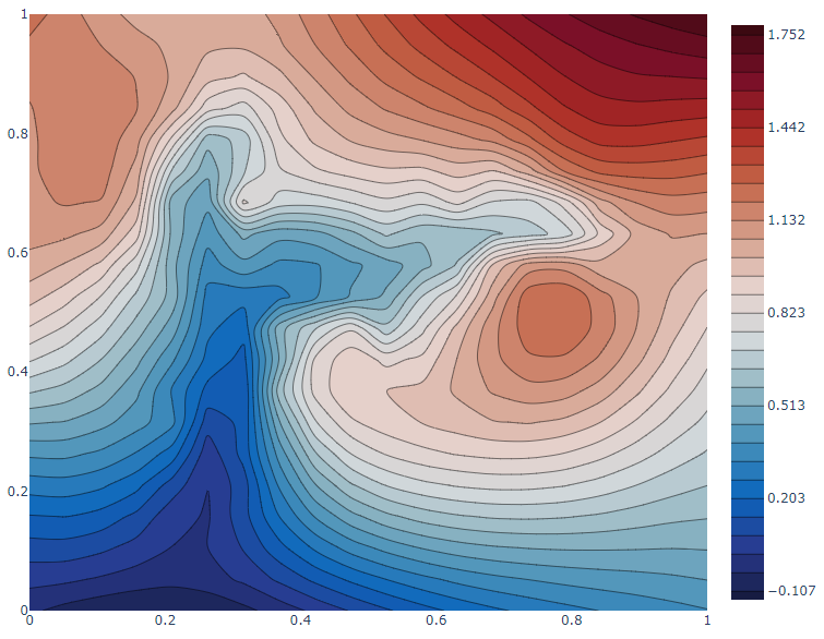
(a)

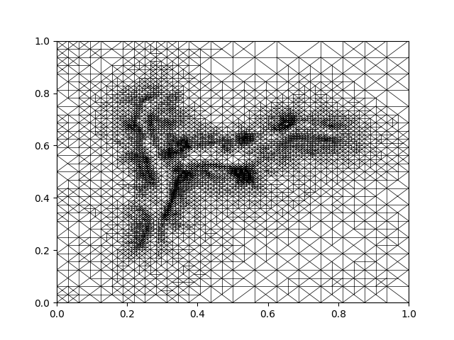
(b)

Figure 9: (a) Contour map; and (b) adaptive mesh of the Canyon data. (keep it for comparison only)

The convergence of the TPSFEM for the Canyon data is shown in Figure 10. Adaptive meshes are markedly more efficient than uniform meshes in square domains. Finer elements on steep sides and coarser elements on regions without data allow the TPSFEM to achieve high RMSE while retaining efficiency. The oscillatory and smooth regions of the Canyon data show a distinct difference in terms of the roughness of surfaces, which is less affected by weights compared to the Mountain data. Thereby, the performance of the error indicators with different weights is similar in both the square and polygonal domains.

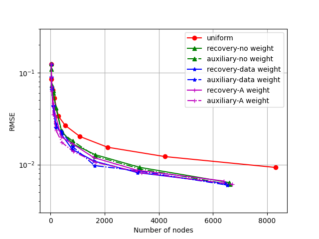
(a)

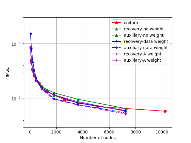
(b)

Figure 10: Convergence of RMSE for the Canyon data in (a) square domains; and (b) polygonal domains.

The advantages of adaptive refinement are weakened in polygonal domains for the Canyon data. The polygonal domain notably reduces the RMSE for the uniform mesh as it is significantly smaller than $[0,1]$ square domains and uniform refinement places fewer nodes on regions without any data points. In contrast, the RMSE of the adaptive meshes is not reduced. Moreover, adaptive meshes with data weight and A weight achieve higher convergence rates than the error indicators not using any weights. Oscillatory regions of this data set inside polygonal domains are near boundaries and may cause over-refinement. Weights help to direct refinement to the interior of the domain where the data density is higher and improve the stability of adaptive refinement.

7.1.3 River Data

The River data is the most complicated data set with various routes and data densities discussed in Section 6. The sampled data concentrates on the river mouth, where the current changes and river beds are eroded by the flow. This leads to oscillatory surfaces and deep holes under the river mouth near point $[0.8,0.6]$ as shown in Figure 12(a). The other regions are relatively smooth and only require coarse elements as shown in Figures 12(b). Only elements near the river mouth are refined with finer elements.

Figure 11: Surface triangulation plot of River data on a polygonal domain.

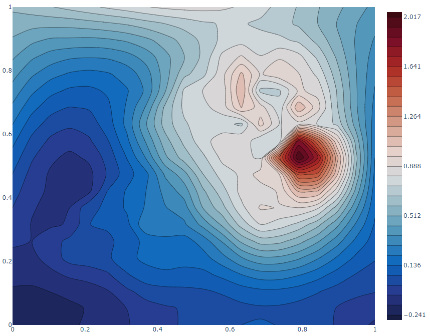
(a)

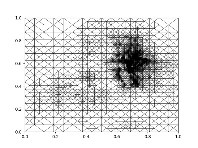
(b)

Figure 12: (a) Contour map; and (b) adaptive mesh of the River data. (keep it for comparison only)

Adaptive meshes in square domains achieve much higher convergence rates compared to uniform meshes for the River data as shown in Figure 13(a). Since the river mouth region is significantly more oscillatory than other regions, adaptive meshes with coarse elements elsewhere are more efficient than uniform meshes similar to the Mountain data. Moreover, the error indicators with or without weights correctly identify the river mouth region and achieve similar performance.

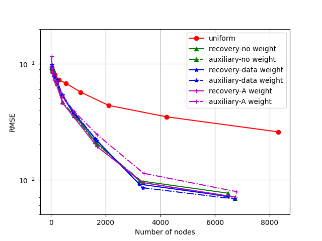
(a)

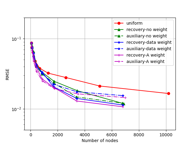
(b)

Figure 13: Convergence of RMSE for the River data in (a) square domains; and (b) polygonal domains.

The convergence for the River data on polygonal domains is shown in Figure 13(b). The efficiency of uniform meshes is improved as it does not refine in regions without data points in polygonal domains similar to the Canyon data. In contrast, adaptive meshes performed poorly in polygonal domains and the RMSE of final adaptive meshes are larger than $10^{-2}$ using 6800 nodes. while the RMSE of adaptive meshes in square domains is about $8\times 10^{-3}$ using 6500 nodes. Since the oscillatory river mouth region is close to the boundaries of the polygonal domain, the error indicators were misled and over-refined near boundaries.

The inconsistencies between boundary conditions and interpolants are enlarged due to the oscillatory regions near domain boundaries near $[0.8,0.6]$ in Figure 14(a). Since the boundary conditions are only approximated using 300 data points, they cannot be as accurate as the TPSFEM in oscillatory areas and the difference leads to high RMSE. The convergence on the trimmed domain is similar to square domains since its river mouth region is far away from boundaries and allows a smoother transition. Note that the auxiliary problem error indicator produces less efficient adaptive meshes in polygonal domains while weights were applied as represented by dashed-dotted lines in Figure 13(b).

Since the River data has the most uneven data distributions out of the three geological surveys, some error indicator values may be dominated by the data densities in applied weights. An example adaptive mesh with finer elements concentrating on the river mouth and nearby rivers is shown in Figure 14(b). These regions have higher data densities and weighted error indicators tend to refine in these regions, which is not effective in reducing the RMSE. Consequently, the efficiency of the adaptive meshes produced by the auxiliary problem error indicator is lower than those of the recovery-based error indicator.

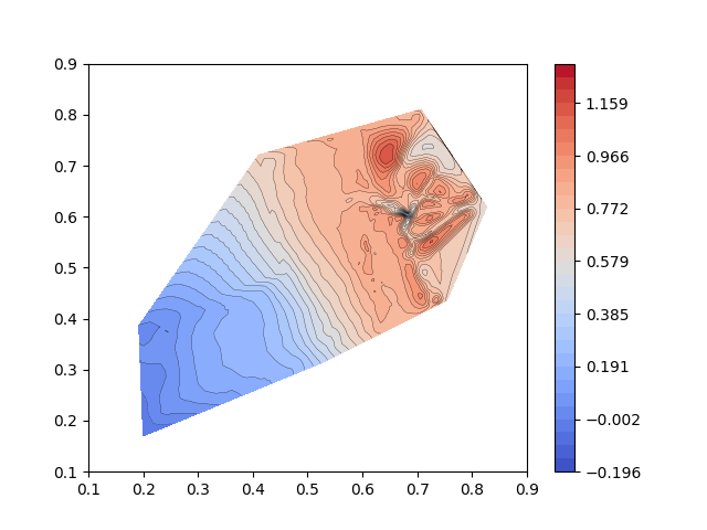
(a)

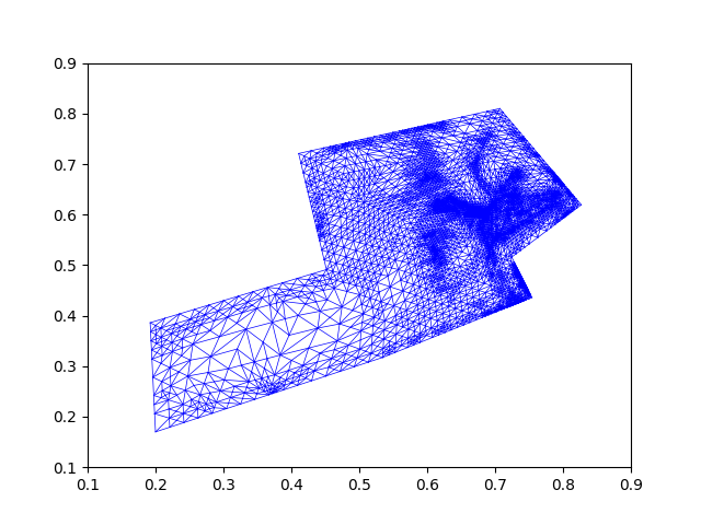
(b)

Figure 14: (a) Contour map of TPSFEM for the River data on a polygonal domain; (b) Adaptive mesh for the River data using data weight.

Overall, adaptive refinement with the two error indicators achieves higher efficiency compared to uniform refinement for both the square and polygonal domains. The polygonal domains shorten the distance between exterior data points and boundaries, which improves the efficiency of uniform meshes. However, it may also lead to inconsistency between the TPSFEM interpolant and approximated boundary conditions, where the accuracy deteriorates. Moreover, it may mislead the error indicators to over-refine near boundaries and weaken the performance of adaptive meshes. Weights of the error indicators cause more spread-out refinement, which helps to prevent over-refinement on oscillatory surfaces near boundaries. However, it also weakens the performance adaptive refinement when the observed data only contains a small portion of oscillatory surfaces.

8 Conclusions

We investigate the performance of the TPSFEM and adaptive refinement on polygonal domains in this article. The DTMs are built using data collected through geological surveys, which often distribute in different shapes that are fitted with polygonal domains. Polygonal domains improve efficiency by fitting the data closely and reducing regions without data points compared to square domains. We use the TPS with a small subset of the data to approximate Dirichlet boundary conditions and alleviate its difference from the interpolant. Additional weights based on data densities were applied to prevent over-refinement near boundaries during adaptive refinement.

Three geological surveys were experimented with to verify the performance of adaptive refinement in polygonal domains. Polygonal domains improve the efficiency of uniform refinement but not adaptive refinement. Despite more accurate boundary conditions, a moderate distance is still required for transition. Otherwise, the accuracy will deteriorate and the error indicators may be misled and cause over-refinement near boundaries. While weights increase the stability of the error indicators, they also weaken the performance of adaptive refinement when the surface is relatively smooth.