Dependence of Molecular Abundance Ratios on the Cosmic Ray Ionization Rate in Nearby Diffuse Clouds

Molecular Abundance Ratios as a Probe of Cosmic Ray Ionization Rate in Diffuse Clouds

Abundance ratios of OH/CO and HCO⁺/CO as probes of the cosmic ray ionization rate in diffuse clouds

Abstract

The cosmic-ray ionization rate (CRIR, $\zeta_{2}$) is one of the key parameters controlling the formation and destruction of various molecules in molecular clouds. However, the current most commonly used CRIR tracers, such as H${}_{3}^{+}$, OH⁺, and H₂O⁺, are hard to detect and require the presence of background massive stars for absorption measurements. In this work, we propose an alternative method to infer the CRIR in diffuse clouds using the abundance ratios of OH/CO and HCO⁺/CO. We have analyzed the response of chemical abundances of CO, OH, and HCO⁺ on various environmental parameters of the interstellar medium in diffuse clouds and found that their abundances are proportional to $\zeta_{2}$. Our analytic expressions give an excellent calculation of the abundance of OH for $\zeta_{2}$ $\leq$10^-15 s^-1, which are potentially useful for modelling chemistry in hydrodynamical simulations. The abundances of OH and HCO⁺ were found to monotonically decrease with increasing density, while the CO abundance shows the opposite trend. With high-sensitivity absorption transitions of both CO (1–0) and (2–1) lines from ALMA, we have derived the H₂ number densities ($n_{\rm H_{2}}$) toward 4 line-of-sights (LOSs); assuming a kinetic temperature of $T_{\rm k}=50\,{\rm K}$, we find a range of (0.14$\pm$0.03–1.2$\pm$0.1)$\times$10² cm^-3. By comparing the observed and modelled HCO⁺/CO ratios, we find that $\zeta_{2}$ in our diffuse gas sample is in the range of $1.0_{-1.0}^{+14.8}$ $\times$10${}^{-16}-2.5_{-2.4}^{+1.4}$ $\times$10^-15 s^-1. This is $\sim$2 times higher than the average value measured at higher extinction, supporting an attenuation of CRs as suggested by theoretical models.

1 Introduction

In the environments of the cold neutral component of the interstellar medium (ISM), where stellar photons cannot penetrate, the low-energy (0.1 $<$ $E$ $<$ 1 GeV) cosmic-rays (CRs) play a critical role in determining the ionization degree, in controlling the thermal balance and for initiating the chemistry at high optical depths (Dalgarno, 2006; Padovani et al., 2013; Vaupré et al., 2014; Grenier et al., 2015). The cosmic-ray ionization rate (CRIR; $\zeta_{2}$) has been measured during the last few decades (Spitzer & Tomasko, 1968; Webber, 1998; Dalgarno, 2006) with the measured value to strongly depend on the adopted methodology (Dalgarno, 2006; Indriolo & McCall, 2012; Indriolo et al., 2015; Bacalla et al., 2019). Various observations found that the CRIR is higher toward the Galactic center (e.g., CMZ, $\zeta_{2}$ = 10^-15 $\sim$ 10^-14 s^-1, Oka et al., 2005; Le Petit et al., 2016a) and supernova remnants (e.g., IC443, W49B, $\zeta_{2}$ $\sim$ 2$\times$10^-15 s^-1, Indriolo et al., 2010; Zhou et al., 2022) than that of nearby molecular clouds (a few 10^-18 $\sim$ 10^-16 s^-1, Caselli et al., 1998; Indriolo & McCall, 2012; Neufeld & Wolfire, 2017). Due to the interaction between CR particles and the ISM, the low-energy CRs attenuate while propagating at higher column densities (Strong et al., 2007; Padovani et al., 2018, 2020). In low-density diffuse clouds (e.g., $n_{\rm H}$ $\sim$ a few hundred cm^-2), CRIR is -on average- almost an order of magnitude higher than that in dense clouds (Indriolo & McCall, 2012).

While $\zeta_{2}$ cannot be easily observed directly, the use of tracers is favored instead. H${}^{+}_{3}$ is one of the most commonly used tracers of the CRIR. It is produced by the CR ionization of H₂ and it is destroyed through reactions with abundant neutral species (e.g., CO, O) and electrons (McCall et al., 1999; Geballe et al., 1999; Dalgarno, 2006; Indriolo & McCall, 2012). The CRIR can be derived once the gas temperature, volume density ($n_{\rm H}$), and column densities (e.g. H₂, CO) are known. Other molecules that are directly relevant to the H${}^{+}_{3}$ chemistry are considered as potential probes of the CRIR, such as HCO⁺ and DCO⁺ (Guelin et al., 1982; van der Tak & van Dishoeck, 2000; Caselli et al., 1998), OH⁺ (Indriolo et al., 2015; Bacalla et al., 2019), and H₂O⁺ (Gerin et al., 2010; Neufeld & Wolfire, 2017; Bialy et al., 2019). Measuring $\zeta_{2}$ with ions such as H${}^{+}_{3}$, OH⁺, and H₂O⁺, requires the presence of bright massive stars in the background, which is not very common. Furthermore, the deuterium species can only be detected in high extinction regions due to its relatively low abundance. Although the above methodology can provide reasonable measurements, it is difficult and somehow impossible for general use.

However, oxygen-bearing molecules have -in principle- the potential to constrain the CRIR; most of the formation of oxygen-bearing species (e.g., OH, HCO⁺) starts from the hydrogenation of ionized oxygen (O⁺). Since the ionization potential of atomic oxygen (13.62 eV) is very close to that of atomic hydrogen (13.6 eV), the majority of oxygen in the cold neutral medium (CNM) is in its atomic form. Thus, in such FUV-shielded regions, O⁺ and oxygen-bearing species are the indirect products of CRs.

OH has long been proposed to be an alternative tracer of molecular gas due to its fairly constant abundance in the ISM (Liszt & Lucas, 1998, 2002; Xu & Li, 2016; Li et al., 2018). The thermal emission and absorption lines of OH 18 cm have been detected extensively toward the CNM, which is extended to the outskirts of the molecular clouds and where the CO emission is faint or undetectable (Turner, 1979; Magnani et al., 1988; Wannier et al., 1993; Cotten et al., 2012; Li et al., 2018; Busch et al., 2021). HCO⁺, in the traditional sense, is a dense gas tracer in the ISM. However, recent observations found that HCO⁺ is ubiquitous in diffuse and translucent clouds (Pety et al., 2017; Luo et al., 2020), especially with absorption measurements against strong continuum sources (e.g., quasars, H ii regions).

In this paper, we combine absorption observations of HCO⁺, and absorption and emission observations of CO to calculate their column densities along each LOS. We attempt to find the chemical connection between these oxygen-bearing molecules (CO, OH, and HCO⁺) that are ubiquitous in diffuse clouds. We investigate the variance of chemical abundances of oxygen-bearing molecules under different environmental parameters (e.g., gas volume density, FUV intensity, CRIR), especially the potential connection of their molecular abundance ratios as a probe of CRIR.

This paper is organized as follows. The observations and archival data used in this work are presented in Section 2. We present the results of column densities and constraints on the gas density in Section 3. In Section 4, we perform photodissociation region (PDR) modelling of CO, OH, and HCO⁺ under various environmental parameters. We discuss the chemistry of CO, OH, and HCO⁺ in the diffuse cloud and derive the chemical abundances in chemical equilibrium in Section 5. We derive the abundance ratios of OH/CO and HCO⁺/CO and constrain the CRIR by combining the observed HCO⁺-to-CO abundance ratio and chemical models in the low-density ($n_{\mathrm{H}}$ $\sim$ 10² cm^-3) diffuse cloud in Section 6. The main results and conclusions are summarized in Section 7.

2 Observations and Data

2.1 HCO⁺ (1–0) and CO (1–0)

The HCO⁺ (1–0) and CO (1–0) absorption observations toward 13 strong continuum sources were carried out during Apr. 2016 to May. 2016 with ALMA (project ID: 2015.1.00503.S, PI: L. Bronfman). The calibration of the raw data was performed using the Common Astronomy Software Applications (McMullin et al., 2007). Self-calibration was performed toward 2 sources (3C454.3 and 3C120) to increase the signal-to-noise ratio and eliminate the spectral contamination from bandpass calibrators. For each line-of-sight (LOS), we decompose the absorption spectra ($\tau_{\nu}$) into different Gaussian components to derive the column density at each velocity component. A detailed description of observations and data reduction can be found in Luo et al. (2020).

The HCO⁺ (1–0) integrated optical depth (in units of km s^-1) and CO (1–0) emission toward another 15 sources are taken from Table 1 in Liszt & Gerin (2023). The original data of HCO⁺ absorption was presented in Lucas & Liszt (1996), Liszt & Lucas (2000), and Liszt & Gerin (2018). We exclude sources in which the brightness temperature of CO is bright ($T_{\rm mb}$ $\geq$ 5 K) since we only focus on diffuse LOSs.

2.2 CO (2–1) data

The CO (2–1) absorption spectra toward 4 sources (3C454.3, 0607-157, 1730-130, and 1741-038) are taken from a blind survey of the absorption lines of bandpass calibrators in ALMA regular observations (Luo et al. 2023, in prep). The data reduction follows the same procedures as that of CO (1–0).

2.3 Reddening $E$(B-V) data

The $E$(B-V) data is taken from Green et al. (2019), in which the values were derived by combining stellar photometry from Pan-STARRS 1 and 2MASS, and parallaxes from Gaia. We use the $E$(B-V) values to derive the total gas column density along the LOS.

3 Results

3.1 Constraints on the gas densities

For those components where both CO (1–0) and (2–1) transitions are available, we use the non-LTE radiative transfer code radex (van der Tak et al., 2007) to constrain the gas densities along the LOSs. We account for H₂ as the main colliding partner of CO. We perform several models covering H₂ volume densities of 10¹ $\leq$ $n_{\rm H_{2}}$ $\leq$ 10⁴ cm^-3, CO column densities of 10¹¹ $\leq$ $N_{\rm CO}$ $\leq$ 10¹⁶ cm^-2 and kinetic temperatures of $10^{1}\leq T_{\rm k}\leq 10^{2}\,{\rm K}$. We then find the optimum solutions by maximizing the likelihood function using the Markov chain Monte Carlo (MCMC) method, which is encoded in $emcee$ (Foreman-Mackey et al., 2013). The likelihood function is defined as:

$$\rm ln\ p=-\frac{1}{2}\sum_{i}\left[\frac{\left(\tau_{obs}^{i}-\tau_{model}^{i}\right)^{2}}{{\sigma^{i}_{obs}}^{2}}+ln\left(2\pi{\sigma^{i}_{obs}}^{2}\right)\right],$$ (1)

where the ${\rm\tau_{obs}^{i}}$ and ${\rm\sigma^{i}_{obs}}$ are the optical depth and uncertainty of the observed i-th transition, respectively. ${\rm\tau_{model}^{i}}$ is the modelled optical depth by radex.

The representative optimum results of $n_{\rm H_{2}}$ under different $T_{\rm k}$ are shown in the left panel of Fig. 1. As $T_{\rm k}$ increases by a factor of 10, the resultant $n_{\rm H_{2}}$ decreases by a factor of 2$\sim$5. However, the column densities are less influenced by $T_{\rm k}$ and vary by $<$4% (for CO) and $<$0.1% (for HCO⁺) (with respect to the values at $T_{\rm k}$=50 K, as shown in the middle and right panels of Fig. 1.)

Figure 1: Left: The optimum $n_{\rm H_{2}}$ solutions at specific $T_{\rm k}$. Different line curves denote results from different sources. Shaded areas represent 1$\sigma$ uncertainties. Middle: Dependence of relative uncertainties (with respect to the values at $T_{\rm k}$=50 K) of column densities of CO on the $T_{\rm k}$. Right: The same as the middle panel but for HCO⁺.

Table 1 summarises the derived $n_{\rm H_{2}}$ and $n_{\rm H}$ of each velocity component at $T_{\rm k}$ = 10, 50, and 100 K. The derived $n_{\rm H_{2}}$ is in the range of (0.11$\pm$0.01–4.4$\pm$0.4)$\times$10² cm^-3.

Table 1: Optical depths of CO (1–0) and (2–1); H₂ density derived from MCMC runs.

Sources	Velocity	$\tau_{\rm CO}$			$n_{\rm H_{2}}$/102 cm-3
	km s-1	1–0	2–1		$T_{\rm k}$=10	50	100 K
	-10.46$\pm$0.04	0.055$\pm$0.002	0.027$\pm$0.002		2.5$\pm$0.7	0.7$\pm$0.2	0.5$\pm$0.1
3C454.3	-9.47$\pm$0.01	0.419$\pm$0.004	0.248$\pm$0.007		3.6$\pm$0.3	1.0$\pm$0.1	0.68$\pm$0.04
	-8.94$\pm$0.01	0.149$\pm$0.003	0.092$\pm$0.004		4.4$\pm$0.4	1.2$\pm$0.1	0.81$\pm$0.07
J0609-1542	7.37$\pm$0.02	0.12$\pm$0.02	0.032$\pm$0.007		0.3$\pm$0.3	0.2$\pm$0.1	0.18$\pm$0.09
J1733-1304	5.03$\pm$0.01	1.55$\pm$0.04	0.553$\pm$0.004		0.46$\pm$0.10	0.14$\pm$0.03	0.11$\pm$0.01
J1743-0350	3.89$\pm$0.05	0.17$\pm$0.01	0.06$\pm$0.02		0.49$\pm$0.53	0.26$\pm$0.18	0.21$\pm$0.12
	5.6$\pm$0.5	0.065$\pm$0.007	0.039$\pm$0.008		3.2$\pm$2.6	0.9$\pm$0.6	0.6$\pm$0.4

3.2 Calculation of column densities

For the rest of the components where only CO (1–0) and HCO⁺ (1–0) are available, we consider an excitation temperature of $T_{\rm ex}=4\,{\rm K}$ for CO and $T_{\rm ex}=2.73\,{\rm K}$ for HCO⁺ (e.g. Liszt & Lucas, 1996; Godard et al., 2010; Luo et al., 2020).

The column densities are calculated with (Mangum & Shirley, 2015):

$$N_{tot}=\frac{3h}{8{\pi}^{3}\left|\mu_{lu}\right|^{2}}\frac{Q_{rot}}{g_{u}}\frac{e^{\frac{E_{u}}{kT_{ex}}}}{e^{\frac{h\nu}{kT_{ex}}}-1}\int\tau_{\nu}d\upsilon,$$ (2)

where $\mathrm{\left|\mu_{lu}\right|^{2}}$ is the dipole matrix element, $\mathrm{Q_{rot}}$ is the rotational partition function, $\mathrm{g_{u}}$ is the degeneracy of the upper energy level, and $\mathrm{E_{u}}$ is the energy of the upper energy level. For each transition, the $\mathrm{\left|\mu_{lu}\right|^{2}}$, $\mathrm{E_{u}}$, and the rest frequency $\nu$ are taken from the CDMS database (Müller et al., 2001, 2005). For linear molecules, the partition function is given by (McDowell, 1987):

$$Q_{tot}=\frac{kT_{\rm ex}}{hB_{0}}e^{\frac{hB_{0}}{3kT_{\rm ex}}},$$ (3)

where $B_{0}$ is the rigid rotor rotation constant. The calculated column densities of CO and HCO⁺ are summarised in Table 2.

Table 2: The $E$(B-V) values, column densities of CO and HCO⁺, fit parameters from 3d-pdr models (see Section 6.3).

Sources	$E$(B-V)	$N_{\rm CO}$	$N_{\rm HCO^{+}}$	Fit parameters
	mag	1014 cm-2	1011 cm-2	$n_{\rm H}$/102 cm-3	$\zeta_{2}$/10-15 s-1
3C454.3 V1	0.106$\pm$0.002	0.84$\pm$0.03	1.41$\pm$0.03	$1.0_{-0.7}^{1.0}$	$1.85_{-1.66}^{0.30}$(*)
3C454.3 V2	0.106$\pm$0.002	3.35$\pm$0.03	3.54$\pm$0.09	$1.0_{0.0}^{0.0}$	$1.58_{-0.26}^{0.26}$(*)
3C454.3 V3	0.106$\pm$0.002	1.03$\pm$0.02	1.09$\pm$0.14	$1.3_{-0.6}^{1.9}$	$0.12_{-0.02}^{2.81}$(*)
J0609-1542	0.203$\pm$0.004	0.52$\pm$0.07	6.82$\pm$0.21	$0.1_{0.0}^{0.0}$	$0.14_{-0.02}^{0.05}$
J1733-1304	0.513$\pm$0.009	11.40$\pm$0.33	17.41$\pm$0.49	$0.3_{0.0}^{0.0}$	$0.34_{-0.06}^{0.06}$
J1743-0350 V1	0.530$\pm$0.008	2.79$\pm$0.19	7.34$\pm$1.23	$0.3_{-0.2}^{0.4}$	$0.25_{-0.18}^{0.38}$(*)
J1743-0350 V2	0.530$\pm$0.008	2.28$\pm$0.24	4.97$\pm$0.56	$0.5_{-0.4}^{0.3}$	$0.25_{-0.20}^{0.75}$(*)
3C120	0.265$\pm$0.006	1.14$\pm$0.24	2.71$\pm$0.58	$0.8_{-0.7}^{0.8}$	$1.17_{-1.14}^{0.42}$(*)
J1745-0753 V1	0.672$\pm$0.008	2.18$\pm$0.89	1.27$\pm$0.87	$3.2_{-3.1}^{28.5}$	$0.86_{-0.86}^{9.14}$(*)
J1745-0753 V2	0.672$\pm$0.008	8.06$\pm$1.26	5.60$\pm$2.46	$1.0_{-0.9}^{2.2}$	$0.86_{-0.81}^{3.12}$(*)
J1745-0753 V3	0.672$\pm$0.008	0.11$\pm$0.32	2.22$\pm$1.20	$0.2_{-0.1}^{1.8}$	$0.10_{-0.10}^{1.48}$(*)
J0211+1051	0.097$\pm$0.006	5.71$\pm$0.40	8.43$\pm$0.32	$0.5_{0.0}^{0.0}$	$0.54_{-0.09}^{0.09}$
J0325+2224	0.239$\pm$0.008	14.92$\pm$0.81	11.21$\pm$0.19	$0.3_{0.0}^{0.0}$	$0.34_{-0.06}^{0.06}$
J0356+2903	0.159$\pm$0.003	25.71$\pm$0.67	16.64$\pm$1.00	$31.6_{-15.8}^{0.0}$	$0.34_{-0.34}^{0.06}$
J0401+0413	0.230$\pm$0.009	3.02$\pm$0.76	5.44$\pm$0.23	$0.2_{-0.1}^{0.6}$	$0.34_{-0.26}^{0.52}$(*)
J0403+2600	0.141$\pm$0.002	9.84$\pm$1.06	6.66$\pm$0.32	$0.6_{0.0}^{0.2}$	$0.74_{-0.10}^{0.12}$(*)
J0406+0637	0.248$\pm$0.006	10.00$\pm$0.63	5.99$\pm$0.57	$0.8_{-0.2}^{0.2}$	$1.00_{-0.37}^{0.17}$(*)
J0407+0742	0.159$\pm$0.006	3.02$\pm$0.67	5.88$\pm$0.34	$0.4_{-0.2}^{0.2}$	$0.63_{-0.47}^{0.10}$(*)
J0426+2327	0.292$\pm$0.008	76.82$\pm$0.71	28.51$\pm$0.63	$31.6_{-15.8}^{0.0}$	$0.18_{-0.10}^{0.11}$
J0427+0457	0.292$\pm$0.017	6.19$\pm$0.71	6.88$\pm$0.27	$0.3_{-0.2}^{0.3}$	$0.54_{-0.38}^{0.19}$(*)
J0437+2037	0.451$\pm$0.006	10.63$\pm$0.41	17.09$\pm$0.81	$0.3_{0.0}^{0.0}$	$0.34_{-0.06}^{0.06}$
J0431+1731	0.354$\pm$0.004	11.11$\pm$0.78	11.21$\pm$1.22	$0.5_{-0.1}^{0.0}$	$0.54_{-0.14}^{0.09}$(*)
J0440+1437	0.442$\pm$0.005	13.17$\pm$0.46	13.42$\pm$0.34	$0.4_{-0.1}^{0.0}$	$0.46_{-0.12}^{0.07}$
J0449+1121	0.398$\pm$0.009	3.65$\pm$0.52	7.21$\pm$0.24	$0.2_{-0.1}^{0.2}$	$0.29_{-0.19}^{0.17}$(*)
J0502+1338	0.371$\pm$0.003	39.04$\pm$0.49	20.08$\pm$0.65	$31.6_{0.0}^{0.0}$	$10.00_{-1.61}^{1.61}$
J0510+1800	0.212$\pm$0.008	2.70$\pm$0.57	1.44$\pm$0.06	$0.8_{-0.5}^{2.4}$	$2.51_{-2.35}^{1.47}$(*)

4 Photodissociation region modelling

Variations in chemical abundances can be used as a diagnostic tool for estimating the environmental parameters of the ISM. To better understand the response of the abundances of the molecular species we examine (CO, OH, HCO⁺) and which are ubiquitously detected in diffuse and translucent clouds, we perform chemical simulations under a range of different environmental parameters (e.g. varying densities, FUV intensities, and cosmic-ray ionization rates). For these calculations, we use the publicly available code 3d-pdr (Bisbas et al., 2012).

In our modelling, we use a suite of one-dimensional uniform slabs with densities of $n_{\rm H}=10^{m}\,{\rm cm}^{-3}$ where $m=2.0,2.5,3.0,3.5$, interacting with four FUV intensities $\chi$/$\chi_{0}$=1,10,30,100 (where $\chi$ is normalized to the spectrum of Draine 1978), and four CRIR $\zeta_{2}=(5,10,50,100)\times$10${}^{-17}\,{\rm s}^{-1}$. The FUV radiation field is considered as plane-parallel that impinges from one direction. The diffuse component of radiation is not accounted for. The maximum value of $A_{\mathrm{V}}$ in our simulations is 20 mag. The gas-phase element abundances relative to hydrogen are shown in Table 3. We set all of the element carbon in the ionized phase with an abundance of 1.4$\times$10^-4 and 60% of the total hydrogen in the molecular phase as the initial conditions in our PDR models (see Röllig et al., 2007, for further details). Throughout the text, the diffuse cloud is referred to as molecular gas with $n_{\rm H}$ $\leq$500 cm^-3 and $A_{\rm V}$ $\leq$1 mag, the translucent cloud is referred to 500$\leq$ $n_{\rm H}$ $\leq$5000 cm^-3 and $A_{\rm V}$ $\leq$5 mag.

Table 3: The gas phase elemental abundances relative to hydrogen in the PDR models.

Elements	Abundance	Elements	Abundance
C+	1.4$\times$10-4	H2	3$\times$10-1
He	1$\times$10-1	H	4$\times$10-1
O	3$\times$10-4

Figure 2 shows our simulation results for a fixed $\zeta_{2}=10^{-16}\,{\rm s}^{-1}$, in which the relative abundance of each species to H₂ is defined as the ratio of the corresponding column densities along the LOS. The variance of CO abundance is shown in the first row of Fig. 2. CO is mostly photodissociated, especially at lower extinction regions (e.g., $A_{\rm V}$ $<$1 mag). As a consequence, the abundance of CO at low $A_{\rm V}$ decreases by two orders of magnitude (from $\sim$ 10^-7 to $\sim$ 10^-9) as the FUV intensity increases from $\chi$/$\chi_{0}$=1 to 100. The abundance of CO increases with increasing $A_{\rm V}$ (e.g., 0.6$\leq$ $A_{\rm V}$ $\leq$5 mag) due to FUV shielding by dust and also self-shielding. However, the abundance of CO slightly decreases by a factor of a few from low to intermediate extinctions ($A_{\rm V}$ $\leq$0.6 mag), which is due to the decrease of the abundance of its precursors (see Section 5). For a fixed FUV intensity, the abundance of CO increases with increasing density. The divergence of CO abundance at different densities is smaller (within a factor of a few, from 5$\times$10^-8 to 5$\times$10^-7 for $\chi$/$\chi_{0}$ = 1) at low extinction ($A_{\rm V}$ $<$1 mag) but larger, over an order of magnitude, at high $A_{\rm V}$. At high-density or low FUV intensity models, the abundance of CO reaches the canonical value (e.g., $\sim$10^-4 as in the solar neighborhood) at lower extinction ($A_{\rm V}$ = 2 mag for $\chi$/$\chi_{0}$ = 1 and $n_{\rm H}$ = 10^3.5 cm^-3) than that of low-density or high FUV intensity models ($A_{\rm V}$ = 5 mag for $\chi$/$\chi_{0}$ = 10 and $n_{\rm H}$ = 10^3.5 cm^-3).

On the contrary, the abundance of OH has a different pattern to that of CO, as shown in the second row of Fig. 2. At low $A_{\rm V}$ (e.g., $\lesssim$2 mag), the abundance of OH increases with the increasing FUV intensity, especially for high-density simulations (e.g., $n_{\rm H}$ = 10^3.5 cm^-3). It increases from $\sim$10^-9 to 10^-8 as the FUV intensity increases from $\chi$/$\chi_{0}$=1 to 100. The abundance of OH decreases with the increasing $A_{\rm V}$ when $A_{\rm V}$ $<$2 mag. The slope of the decreasing trend of OH abundance with $A_{\rm V}$ becomes larger for lower densities and higher FUV intensities. As can be seen from Fig. 2, the abundance of OH decreases by a factor of 2 for the high-density ($n_{\rm H}$ = 10^3.5 cm^-3) and low FUV intensity ($\chi$/$\chi_{0}$=1) model, while it decreases by two orders of magnitude for the low-density ($n_{\rm H}$ = 10² cm^-3) and high FUV intensity ($\chi$/$\chi_{0}$=100) model.

The knee point where the OH abundance trend turns, is approximately at an $A_{\rm V}$ of 2 mag, after which it monotonically decreases with the increase of density below the $A_{\rm V}$ value, while it converges above the $A_{\rm V}$ value (except for $n_{\rm H}$ = 10^3.5 cm^-3). Particularly, the divergence of OH abundance at low FUV intensities is larger than that of at high FUV intensity. With the density increase from 10² cm^-3 to 10³ cm^-3, the abundance of OH decreases by nearly two orders of magnitude at $\chi$/$\chi_{0}$=1, while it decreases only less than one order of magnitude at $\chi$/$\chi_{0}$=100.

Furthermore, the abundance of HCO⁺ follows a similar trend to that of OH at low FUV intensity; HCO⁺ decreases with the increase of density and $A_{\rm V}$ ($A_{\rm V}$ $<$2 mag). While this trend is maintained for the high-density (e.g., $n_{\rm H}$ $>$10³ cm^-3) and low FUV intensity models (e.g., $\chi$/$\chi_{0}$ $<$100), the abundance of HCO⁺ declines at low extinction for low-density and high FUV intensity models. At high FUV intensities, HCO⁺ does not form as efficiently as OH does. The difference between HCO⁺ and OH is most likely due to the interruption of the formation of HCO⁺ through the OH channel at high FUV intensities (see Section 5).

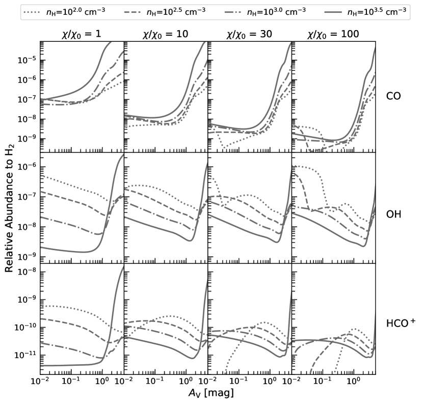
Figure 2: The chemical abundances of CO, OH, and HCO⁺ as a function of $A_{\rm V}$ using 3d-pdr for four densities ($n_{\mathrm{H}}$ = 10², 10^2.5, 10³, and 10^3.5 cm^-3) and four FUV intensities ($\chi$/$\chi_{0}$ = 1, 10, 30, 100) for a fixed CRIR of $\zeta_{2}=10^{-16}\,{\rm s}^{-1}$.

Figure 3 shows our simulations with a constant FUV intensity ($\chi$/$\chi_{0}$=1). The abundances of CO, OH, and HCO⁺ have a similar trend as $\zeta_{2}$ varies: they increase with increasing CRIR at low extinction (e.g., $A_{\rm V}$ $<$ 1 mag for CO at $n_{\rm H}$=10³ cm^-3), while they have an inverse relation at high extinctions. The abundance of CO increases by an order of magnitude as the CRIR increase from 10^-16 to 10^-15 s^-1 at low extinctions for low-density models (e.g., $n_{\rm H}$ $\leq$10³ cm^-3). The $A_{\rm V}$ value of the “inverse point” where the dependence of CO abundance on the CRIR turns opposite, is higher ($A_{\rm V}$ $\sim$5 mag) for low-density models and lower ($A_{\rm V}$ $\sim$0.3 mag) for high-density models. For the $n_{\rm H}$ = 10^3.5 cm^-3 models, an order of magnitude increase in CRIR (from $\zeta_{2}=10^{-16}\,{\rm s}^{-1}$ to $10^{-15}\,{\rm s}^{-1}$) affects the CO abundance from a factor of $\sim 2$ at low $A_{\rm V}$ to $\gtrsim 10^{2}$ at higher $A_{\rm V}$.

As an important ISM environmental parameter, the CRIR has a high impact on the abundance of OH. In particular, it is almost proportional to $\zeta_{2}$ at low $A_{\rm V}$. As seen in the second row of Fig. 3, the abundance of OH increases by an order of magnitude as $\zeta_{2}$ increases from 10^-16 to 10^-15 s^-1 at low $A_{\rm V}$ (e.g., $A_{\rm V}$ $<$1 mag) for all four densities explored. The $A_{\rm V}$ value of the “inverse point” is larger than that of CO, which decreases with increasing density. At high extinction ($A_{\rm V}$ $>$2 mag) and high-densities ($n_{\rm H}$ $>$10³ cm^-3), the abundance of OH decreases with the increasing $\zeta_{2}$.

The dependence of HCO⁺ abundance on the CRIR is similar to that of OH. With the CRIR increase by an order of magnitude, the abundance of HCO⁺ increases by an order of magnitude at low $A_{\rm V}$ for $n_{\rm H}$ $\leq$10³ cm^-3. However, at low-density models ($n_{\rm H}$ = 10² cm^-3), an increase of CRIR from 5$\times$10^-16 s^-1 to 10^-15 s^-1 only results in a slight increase ($\leq$30%) on the abundance of HCO⁺, meaning that the abundance of HCO⁺ would hit a maximum value in this case (see Section 5.2 for more discussion). At high-densities ($n_{\rm H}\sim$10^3.5 cm^-3), the increase of CRIR by an order of magnitude increases HCO⁺ abundance by a factor of $\sim$5. The $A_{\rm V}$ value of the “inverse point” is the same as that of OH.

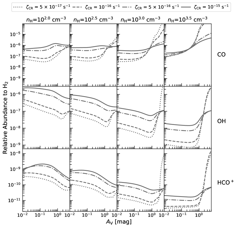
Figure 3: As in Fig. 2 but for a fixed FUV intensity of $\chi/\chi_{0}=1$.

5 Analysis and Discussion

5.1 The abundance of OH in diffuse cloud

In diffuse clouds, the formation of OH can be traced back from two channels that form OH⁺. The first one starts from the charge transfer reaction:

$$\rm H^{+}+O\rightarrow O^{+}+H,$$ (R1)

with O⁺ forming OH⁺ through reaction:

$$\rm O^{+}+H_{2}\rightarrow OH^{+}+H.$$ (R2)

In addition to the reactions R1 and R2, atomic oxygen can directly react with H${}_{3}^{+}$ to form OH⁺ (the second channel):

$$\rm O+H_{3}^{+}\rightarrow OH^{+}+H_{2}.$$ (R3)

Once OH⁺ has formed, it can hydrogenate to form the precursors of OH, namely H₂O⁺ and H₃O⁺:

$$\rm OH^{+}+H_{2}\rightarrow \ \rm H_{2}O^{+}+H,$$ (R4)

$$\rm H_{2}O^{+}+H_{2}\rightarrow \ \rm H_{3}O^{+}+H,$$ (R5)

in which reaction R4 is the main destruction process for OH⁺. OH is formed through electron recombination reactions:

$$\rm H_{2}O^{+}+e\rightarrow \ \rm OH+H,$$ (R6)

$$\rm\rightarrow \ \rm O+H_{2}+H,$$ (R7)

$$\rm\rightarrow \ \rm O+H+H,$$ (R8)

and

$$\rm H_{3}O^{+}+e\rightarrow \ \rm OH+H+H,$$ (R9)

$$\rm\rightarrow \ \rm OH+H_{2},$$ (R10)

$$\rm\rightarrow \ \rm H_{2}O+H.$$ (R11)

From reaction R11, H₂O also contributes to the formation of OH by photodissociation:

$$\rm H_{2}O+h\nu\rightarrow OH+H.$$ (R12)

Reaction R12 is also the main destruction path of H₂O. The minor destruction path of H₂O is through C⁺ in diffuse clouds:

$$\rm H_{2}O+C^{+}\rightarrow HCO^{+}+H.$$ (R13)

The destruction of OH in diffuse clouds includes photodissociation:

$$\rm OH+h\nu\rightarrow O+H,$$ (R14)

reaction with C⁺:

$$\rm OH+C^{+}\rightarrow CO^{+}+H,$$ (R15)

$$\rm OH+C^{+}\rightarrow CO+H^{+},$$ (R16)

and reaction with H⁺:

$$\rm OH+H^{+}\rightarrow OH^{+}+H.$$ (R17)

The OH abundance ($x$(OH)=$n$(OH)/$n_{\rm H}$) in chemical equilibrium can be solved when the formation and destruction processes reach a balance (see detailed derivation in Appendix A). In diffuse clouds, photodissociation dominates the destruction of OH, and reactions R15 and R16 play a minor role. Since the abundance of C⁺ is an order of magnitude higher than H⁺ when the $\zeta_{2}$ is not high (e.g., $\zeta_{2}$ $\lesssim$10^-15 s^-1, Le Petit et al., 2016b), we ignore here the contribution from R17 (the last term in equation A17). Thus, the abundance of OH can be written as:

$$\rm{\it x}(OH)= \ \rm\frac{{\it x}(O)\zeta_{2}\theta}{k_{pd}(R14)+{\it n}(C^{+})(k_{R15}+k_{R16})}$$

$$\ \rm\times[1-\frac{{\it n}(H_{2})k_{R5}\delta+{\it n}(e)(k_{R7}+k_{R8})}{{\it n}(H_{2})k_{R5}+{\it n}(e)(k_{R6}+k_{R7}+k_{R8})}]$$

$$= \ \rm\frac{{\it x}(O)\zeta_{2}\theta\phi}{k_{pd}(R14)+{\it n}(C^{+})(k_{R15}+k_{R16})},$$ (4)

where $\phi$ is the term in the square brackets of equation 4 and $\theta$ is in the form of equation A15. Since the term $\delta$ is small ($\sim$0.1) in average diffuse ISM conditions (e.g., T =30 K, $A_{\rm V}$ = 1 mag), $\phi$ $\approx$1. To a good approximation, equation 4 can be simplified as:

$$\rm{\it x}(OH)= \ \rm\frac{{\it x}(O)\zeta_{2}\theta}{k_{pd}(R14)+{\it n}(H){\it x}(C^{+})(k_{R15}+k_{R16})}.$$ (5)

Since there is an anti-correlation between x(OH) and $n_{\mathrm{H}}$ as density increases, the abundance of OH decreases monotonically ( similar to that shown in Fig. 2). On the other hand, if the UV radiation field increase or the extinction decreases, the gas temperature will increase. Therefore, all reaction rates in equation 5 will decrease and, therefore, the abundance of OH will also increase.

As can be seen from equation 5, the abundance of OH is proportional to $\zeta_{2}$ in the diffuse cloud. Figure 4 shows the resultant abundance of OH ($A_{\rm V}$ = 1 mag, $n_{\rm H}$ = 10² cm^-2) from both equations 5 as well as the 3d-pdr models, in which the reaction rates are taken from McElroy et al. (2013). It should be emphasized that equation 5 can only be used under average ISM conditions. At high FUV radiation fields or very low $A_{\rm V}$, the main formation pathway of OH is contributed by neutral-neutral reactions through atomic O and H, which are not included in our analysis. Equation 5 represents a good approximation ( with $<$60% uncertainty) for $\zeta_{2}$ $<$10^-15 s^-1 when compared with 3d-pdr models.

However, in the PDR simulations, the abundance of OH reaches the maximum at $\zeta_{2}$ $\sim$ 2$\times$10^-15 s^-1. For higher $\zeta_{2}$, the OH abundance decreases. This is because the destruction of OH at high CRIR is dominated by H⁺ (Reaction R17) rather than by photodissociation and C⁺ (Reactions R14$\sim$R16), which has been ignored in deriving equation 5. Similar work using isothermal simulations has been reported by Bisbas et al. (2017, their Fig. 10), in which the OH abundance peaks at $\zeta_{2}$/$n_{\rm H}$ $\approx$ 2$\times$10^-17 cm³ s^-1.

Though there are limitations, we still highlight the usage of equation 5 at $\zeta_{2}$ $<$10^-15 s^-1 instead of running chemical networks, especially when coupled with hydrodynamical simulations, as this dramatically reduces the overall computational expense.

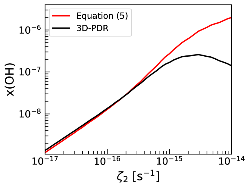
Figure 4: The value of x(OH) as a function of CRIR, in which the red curve is obtained from equation 5 and the black curve is from 3d-pdr models. The extinction is at 1 mag and the gas density is 10² cm^-3.

5.2 The abundance of HCO⁺ in diffuse cloud

The formation of HCO⁺ starts from ion-neutral reactions:

$$\rm CO^{+}+H_{2}\rightarrow \ \rm HCO^{+}+H,$$ (R18)

$$\rm C^{+}+H_{2}O\rightarrow \ \rm HCO^{+}+H,$$ (R19)

$$\rm CH+O\rightarrow \ \rm HCO^{+}+e,$$ (R20)

where CO⁺ is the result of reaction R15. Reaction R18 is very efficient as almost all CO⁺ forms HCO⁺.

The destruction of HCO⁺ is always dominated by free electrons:

$$\rm HCO^{+}+e\rightarrow CO+H.$$ (R21)

Thus, in chemical equilibrium, the HCO⁺ abundance ($\rm{\it x}(HCO^{+})$) can be written as:

$$\rm{\it x}(HCO^{+})= \ \rm\frac{{\it x}(C^{+})}{{\it x}(e)k_{R21}}\times[{\it x}(OH)k_{R15}+{\it x}(H_{2}O)k_{R19}$$

$$\ \rm+\frac{{\it x}(O)}{{\it x}(C^{+})}{\it x}(CH)k_{R20}].$$ (6)

By substituting equations A1-A17 to the above and relating $\rm{\it x}(H_{2}O)$ with $\rm{\it x}(OH)$, we obtain:

$$\rm{\it x}(HCO^{+})= \ \rm\frac{{\it x}(C^{+}){\it x}(OH)}{{\it x}(e)k_{R21}}\times[k_{R15}+\epsilon k_{R19}$$

$$\ \rm+\frac{{\it x}(O)}{{\it x}(C^{+})}\frac{{\it x}(CH)}{{\it x}(OH)}k_{R20}],$$ (7)

where $\epsilon$ is:

$$\rm\epsilon= \ \rm[k_{pd}(R14)+{\it n}(H){\it x}(C^{+})(k_{R15}+k_{R16})]\times$$

$$\ \rm\{k_{pd}(R12)+[k_{pd}(R12)+{\it n}(H){\it x}(C^{+})k_{R13}]\times$$

$$\ \rm[\frac{k_{R9}+k_{R10}}{k_{R11}}+\frac{k_{R9}+k_{R10}+k_{R11}}{k_{R11}}\frac{{\it x}(e)k_{R6}}{{\it x}(H_{2})k_{R5}}]\}^{-1}.$$ (8)

For low values of $\zeta_{2}$ (e.g., $\zeta_{2}$ $\lesssim$ 10^-15 s^-1), the production of electrons results primarily from the ionization of atomic carbon. The electron abundance can be, thus, approximated with the C⁺ abundance, e.g. $\rm{\it x}(e)$ = $\rm{\it x}(C^{+})$ (Goldsmith, 2001). If the ionization degree of the cloud is large or the gas density is low, x(O)/x(C⁺) $\approx$ 2, and the abundance of CH is an order of magnitude lower than that of OH. Thus, the contribution from the last term of equation 7 is small. Equation 7 can, then, be simplified as:

$$\rm{\it x}(HCO^{+})\approx \ \rm\frac{{\it x}(OH)}{k_{R21}}\times[k_{R15}+\epsilon k_{R19}].$$ (9)

For higher $\zeta_{2}$ (e.g., $\zeta_{2}$ $\gg$ 10^-15 s^-1), a significant fraction of electrons are produced by H⁺ (Le Petit et al., 2016b). In this case, equation 7 should be applied.

However, we should still keep in mind that at low extinctions and high FUV intensities, the destruction of CO⁺ by H and free electrons becomes more efficient than that of H₂ (Reaction R18). The formation of HCO⁺ is, therefore, interrupted. The response of HCO⁺ abundance does not follow a similar trend to that of OH at low $A_{\rm V}$ and high FUV intensities (as shown in Fig. 2). In such a case, equation 9 is not valid.

Overall, equation 9 shows that $x$(HCO⁺) is proportional to x(OH) in diffuse clouds. High-sensitivity absorption observations found that the integrated optical depth of HCO⁺ has a tight linear relation with that of OH ($N$(HCO⁺)/$N$(OH) = 0.03, Liszt & Lucas, 1996). Considering a diffuse cloud with gas temperature ranging from 50 to 100 K, at an extinction range of $0.5-1.5\,{\rm mag}$, the resultant HCO⁺/OH ratio is nearly constant ($\sim$3.5$\times$10^-3, see Fig. 5). Note that while this value is an order of magnitude lower than the above observations, the abundance of OH measured in diffuse gas has large uncertainty between different LOSs (see Section 5.4 for more discussion). Additionally, most of the HCO⁺ observations of Liszt & Lucas (1996) have high optical depths ($\tau>$1). This means that the formation and destruction of HCO⁺ may be different from what we considered here. Furthermore, the CH abundance in translucent clouds is likely to be comparable to that of OH ($\sim$4$\times$10^-8, Liszt & Lucas, 2002; Sheffer et al., 2008), meaning that the HCO⁺/OH ratio could be underestimated by equation 9.

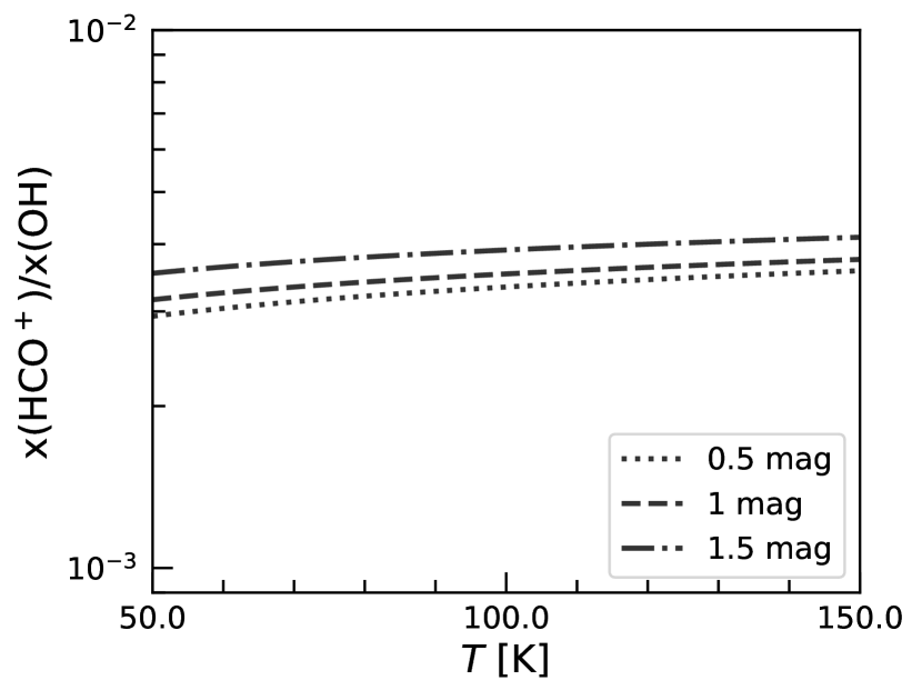
Figure 5: The HCO⁺/OH abundance ratios that calculated from equation 9 at a temperature range of 50–150 K. Different line styles represent the three $A_{\rm V}$ values (0.5, 1.0, and 1.5 mag) that are used in the calculation.

Finally, in the case of a high CO abundance, the latter becomes the precursor of HCO⁺ through reaction:

$$\rm CO+H_{3}^{+}\rightarrow HCO^{+}+H_{2}.$$ (R22)

In this case, the abundance of HCO⁺ may be underestimated.

5.3 The abundance of CO in diffuse cloud

There are three major formation paths of CO: Reactions R16, R21, and

$$\rm CH+O\rightarrow \ \rm CO+H.$$ (R23)

The destruction of CO in the diffuse and translucent clouds is dominated by photodissociation:

$$\rm CO+h\nu\rightarrow \ \rm C+O,$$ (R24)

and by the interaction with He⁺

$$\rm CO+He^{+}\rightarrow \ \rm C^{+}+O+He.$$ (R25)

The CO abundance ($\rm{\it x}(CO)$) in chemical equilibrium can be written as:

$$\rm{\it x}(CO)= \ \rm\frac{{\it n}(H)}{k_{pd}(R24)+\eta_{CO}}[{\it x}(C^{+}){\it x}(OH)k_{R16}+$$

$$\ \rm{\it x}(HCO^{+}){\it x}(e)k_{R21}+{\it x}(CH){\it x}(O)k_{R23}].$$ (10)

$\rm\eta_{CO}$ denotes the destruction rate of CO by He⁺, which is proportional to the CRIR. If we substitute x(HCO⁺) as x(OH) using equation 7, we obtain:

$$\rm{\it x}(CO)= \ \rm\frac{{\it n}(H)}{k_{pd}(R24)+\eta_{CO}}[{\it x}(CH){\it x}(O)(k_{R20}+k_{R23})+$$

$$\ \rm{\it x}(C^{+}){\it x}(OH)(k_{R15}+k_{R16}+\epsilon k_{R19})].$$ (11)

The CO abundance is proportional to the gas density. In low-density diffuse gas where photodissociation dominates the destruction of CO, the OH channels dominate the formation of CO (Luo et al., 2023). Equation 11 can be simplified as :

$$\rm{\it x}(CO)\approx \ \rm\frac{{\it n}(H){\it x}(C^{+}){\it x}(OH)}{k_{pd}(R24)}[(k_{R15}+k_{R16}+\epsilon k_{R19})].$$ (12)

Since $\rm{\it x}(OH)$ is proportional to the CRIR, $\rm{\it x}(CO)$ increases with the increasing CRIR.

5.4 Comparison between the observed molecular abundances and model predictions

Radio emission line observations toward high latitude diffuse clouds (0.4$\lesssim$ $A_{\rm V}$ $\lesssim$1.1 mag) have reported an abundance of OH between 1.6$\times$10^-7 and 4$\times$10^-6 (Magnani et al., 1988). Absorption measurements toward quasars at radio wavelengths suggest a relative abundance ratio to total H column density ($N_{\rm OH}$/$N_{\rm H}$) of $2.5-5\times 10^{-8}$ at $A_{\rm V}$ of 1 mag (Crutcher, 1979; Liszt & Lucas, 1996). Considering that the molecular fraction is 10%-20% at such LOSs (Lucas & Liszt, 1996), the abundance of OH with respect to H₂ is in the range of $\sim$10^-7 to 10^-6. Recent radio observations by Tang et al. (2021) covering a broad range of $A_{\rm V}$ (0.2$-$60 mag) suggest that the abundance of OH is higher ($\sim$10^-6) at low $A_{\rm V}$ and lower ($\sim$10^-7) at higher $A_{\rm V}$. The high spatial resolution ($\sim$0.12 pc) observations by Xu et al. (2016) in the Taurus boundary also found a decreasing trend of OH abundance with the $A_{\rm V}$.

Our models show that the abundance of OH strongly depends on the density distribution and the ISM environmental parameters (see Section 4, Fig. 2 and 3) and can vary by more than two orders of magnitude ($\sim$ 10^-9 $-$ 10^-7 at the same $A_{\rm V}$). As can be seen from equation 5, x(OH) is anti-correlated with ${\rm k_{pd}(R22)}$ and $n_{\rm H}$. This is consistent with the OH survey in nearby molecular clouds of Tang et al. (2021). Considering the aforementioned large scatter of OH abundance in diffuse clouds, we adopt an OH abundance in the range of 10^-7 to 10^-6 as the “typical value”. Thus, for any given FUV intensity (1$\leq$ $\chi$/$\chi_{0}$ $\leq$100) and density (10² $<$ $n_{\rm H}$ $\leq$ 10^3.5 cm^-3), the model underestimates the abundance of OH at an $A_{\rm V}\simeq 0.2-2\,{\rm mag}$ if a $\zeta_{2}=10^{-16}\,{\rm s}^{-1}$ is adopted (Fig. 2). As seen from Fig. 3, the CRIR should be no less than 10^-16 s^-1 if we are to reproduce the observed abundance of OH in diffuse clouds.

Due to the sub-thermal excitation of HCO⁺ transitions in low-density gas (Godard et al., 2010; Luo et al., 2020), its abundance can vary over an order of magnitude without precise measurement of both the excitation temperature and optical depth (Luo et al., 2023). The abundance of HCO⁺ in diffuse clouds has been measured frequently through absorption observations against strong continuum sources (e.g., quasars, H ii regions). Despite the different methods in obtaining the column density of H₂, the abundance of HCO⁺ is fairly constant in diffuse gas ((1.7–3.1)$\times$10^-9, Lucas & Liszt, 1996; Liszt & Gerin, 2016; Gerin et al., 2019; Luo et al., 2020). At a CRIR of 10^-16 s^-1, our models underestimate the abundance of HCO⁺ in diffuse gas in all density and FUV intensity ranges explored (Fig. 2). Therefore, to reproduce the observed abundance of HCO⁺, the gas density should be approximately in the range of 10² $\leq$ $n_{\rm H}$ $\leq$ 10^2.5 cm^-3 and the CRIR should be $\zeta_{2}>10^{-16}\,{\rm s}^{-1}$ (Fig. 3). The inferred density is consistent with the inferred density in Section 3.1 and those by radio and UV absorptions (e.g., 80$-$160 cm^-3, Goldsmith, 2013; Liszt & Gerin, 2016; Luo et al., 2020).

In diffuse clouds, most of the carbon is in the form of C⁺ or C⁰ due to insufficient shielding from UV photons. Similar to HCO⁺, the CO low-$J$ transitions are usually sub-thermally excited in the low-density diffuse gas (Goldsmith et al., 2008; Luo et al., 2020). The abundance of CO in diffuse clouds can vary by two orders of magnitude in different environments (e.g., 2.6$\times$10^-8–2$\times$10^-5 from UV absorption measurements). In particular, it increases with increasing $N_{\rm H_{2}}$ (or $A_{\rm V}$) (Burgh et al., 2007; Liszt, 2007; Sheffer et al., 2008). The abundance of CO through CO (J=1–0) emission line measurements in low extinction regions ($A_{\rm V}\sim 1\,{\rm mag}$) in Taurus is approximately (1.2–7)$\times$10^-6 (Goldsmith et al., 2008; Pineda et al., 2010), which is over an order of magnitude lower than the canonical value in well-shielded regions (e.g., $\sim$10^-4, Frerking et al., 1982). This value is similar to that of absorption observations in diffuse LOSs ($A_{\rm V}$ = 0.19–2.08 mag, $f_{\rm CO}$ = (0.2$\pm$0.1–5$\pm$4)$\times$10^-6, Luo et al., 2020). Our models shown in Fig. 3 can reasonably explain the observed CO abundances.

Considering all the above, we find that the abundances of OH, HCO⁺, and CO in diffuse clouds suggest an ISM environment with low gas densities ($n_{\rm H}$ $\lesssim$10^2.5 cm^-3) and high CRIRs ($\zeta_{2}$ $\gtrsim$10^-16 s^-1). A more quantitative analysis is discussed below (§6.3).

6 The abundance ratios and CRIR in diffuse clouds

As can be seen from equations 5 and 9, the abundances of OH and HCO⁺ are proportional to the CRIR in diffuse gas, which implies they can be used to constrain CRIR with a given density. However, molecular hydrogen does not emit radiation that can be observed from radio telescopes due to the lack of permanent dipole moment, the measurement of an accurate H₂ column density in the CNM, as well as its exact abundance, is very hard. Instead, it is possible to put constraints on the CRIR by combining the observed molecular column densities and their ratios with chemical models.

6.1 The abundance ratio of OH/CO

The abundance ratio of OH/CO can be obtained from equation 11:

$$\rm\frac{{\it x}(OH)}{{\it x}(CO)}= \ \rm\frac{1}{{\it x}(C^{+})(k_{R15}+k_{R16}+\epsilon k_{R19})}\times$$

$$\ \rm[\frac{k_{pd}(R24)+\eta_{CO}}{{\it n}(H)}-\frac{{\it x}(CH)}{{\it x}(CO)}{\it x}(O)(k_{R20}+k_{R23})].$$ (13)

The second term in the square brackets can be safely ignored in the diffuse gas:

$$\rm\frac{{\it x}(OH)}{{\it x}(CO)}\approx \ \rm\frac{k_{pd}(R24)+\eta_{CO}}{{\it n}(H){\it x}(C^{+})(k_{R15}+k_{R16}+\epsilon k_{R19})}.$$ (14)

Figure 6 shows the predicted abundance ratio of OH/CO with the column density of CO ($N_{\rm CO}$) from 1D slab model simulations ($n_{\rm H}$ = 10² cm^-3). The abundance ratio of OH/CO decreases as the increasing $N_{\rm CO}$. The abundance ratio of OH/CO will increase with the increasing FUV intensity by a factor of a few at low $N_{\rm CO}$, while it remains approximately constant at high $N_{\rm CO}$. This is because, at a low FUV intensity (e.g., $\chi$/$\chi_{0}\sim 1$), the gas temperature is significantly lower than that of a moderate FUV intensity (e.g., $\chi$/$\chi_{0}\sim 10$). The decreasing gas temperature would increase the reaction rates of R15, R16, and R19, leading to a lower OH/CO ratio. However, at high $N_{\rm CO}$, CO molecules exist mainly in well-shielded regions, in which the gas temperature does not significantly increase even when high external FUV intensities exist.

As shown in Fig. 6, the abundance ratio of OH/CO monotonically increases with the increasing CRIR at a given $N_{\rm CO}$. Since high CRIR heats the gas, the reaction rates of R15, R16, and R19 will decrease. At the meantime, $\eta_{\rm CO}$ will increase as the increasing CRIR, leading to a higher OH/CO ratio.

The results shown in Fig. 6 indicate that once the gas density can be constrained from line ratios (e.g., C i/CO, CO rotational line ladder), the CRIR can be inferred from OH and CO observations without knowledge of their exact abundance relative to H₂. This is potentially useful in high spatial resolution radio spectral line observations, especially when the column densities of H₂ cannot be determined.

However, the main challenge of generalizing the use of OH and CO as a probe of CRIR is that the excitation temperature of OH is usually within a few K above the Galactic synchrotron background (Li et al., 2018). This will lead to an order of magnitude uncertainty in $N_{\rm OH}$ through emission lines if $T_{\rm ex}$ varies between 0.1–1.0 K above $T_{\rm bg}$ (note that $N_{\rm OH}$ $\propto$ $T_{\rm ex}$/($T_{\rm ex}$-$T_{\rm bg}$)). Absorption measurements are less suffered from the above issues ($N_{\rm OH}$ $\propto$ $T_{\rm ex}$), while the optical depth of OH is usually between a few to tens of 10^-3 (more than an order of magnitude lower than that of HCO⁺). This affects the feasibility of detecting the absorption of OH in a relatively short integration time even with the JVLA. With the proposed capability of high-sensitivity radio telescopes such as FAST, and SKA in the future (McClure-Griffiths et al., 2015), it is possible to constrain the CRIR through OH and CO in both the Milky Way and external galaxies.

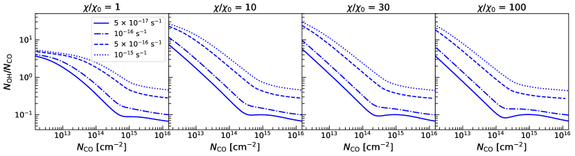
Figure 6: The predicted abundance ratios by PDR models with $n_{\rm H}$ = 10² cm^-3, and different line styles represent the four CRIR values that are used for modelling ($\rm\zeta_{2}$ = 5$\times$10^-17, 10^-16, 5$\times$10^-16, and 10^-15 s^-1). From left to right represent the four representative FUV intensities ($\chi$/$\chi_{0}$ = 1, 10, 30, and 100).

6.2 The abundance ratio of HCO⁺/CO

Contrary to OH, HCO⁺ can be easily detected in diffuse clouds through absorption measurements against strong continuum sources (e.g., a few to tens of minutes with ALMA), and has less uncertainty in calculating its column density.

Following the same way, if we replace equation 9 with equation 14, the abundance ratio of HCO⁺/CO can be written as:

$$\rm\frac{{\it x}(HCO^{+})}{{\it x}(CO)}\approx \ \rm\frac{k_{pd}(R24)+\eta_{CO}}{{\it n}(H){\it x}(C^{+})k_{R21}}[1+\frac{k_{R16}}{k_{R15}+\epsilon k_{R19}}]^{-1}.$$ (15)

Figure 7 shows the predicted abundance ratio of HCO⁺/CO with $N_{\rm CO}$ from 1D slab model simulations ($n_{\rm H}$ = 10² cm^-3), overlaid with the observed values from absorption measurements. Red dots are the observed values, and different line curves represent PDR models under different CRIRs. As seen from Fig. 7, the majority (22 out of the total 26) of the observational values are within $10^{-16}\lesssim\zeta_{2}\lesssim 10^{-15}\,{\rm s}^{-1}$.

At a given $N_{\rm CO}$, the abundance ratio of HCO⁺/CO will first increase with increasing CRIR. This is similar to the variance of OH/CO as we have explained in Section 6.1. With the increasing photodissociation rate (R24) and the gas temperatures, reaction rates R15, R16, R19, and R23 decrease while the reaction rates of electron recombination (R21) increase. Thus, the increasing trend of HCO⁺/CO is slowing down because of the increasing destruction rate of HCO⁺ by free electrons. Consequently, there is a plateau of the HCO⁺/CO ratio (as well as the abundance of HCO⁺), where the increasing CRIR no longer increases the HCO⁺/CO ratio.

However, the HCO⁺/CO ratio decreases at an even higher CRIR. This is because the most important precursors of HCO⁺ (R18), such as CO⁺, are destroyed by atomic hydrogen and free electrons at high temperature, reducing the formation efficiency of HCO⁺. The abundance ratio of HCO⁺/CO reaches a maximum when the CRIR is approximately 10^-15 s^-1 for $n_{\rm H}=10^{2}\,{\rm cm}^{-3}$.

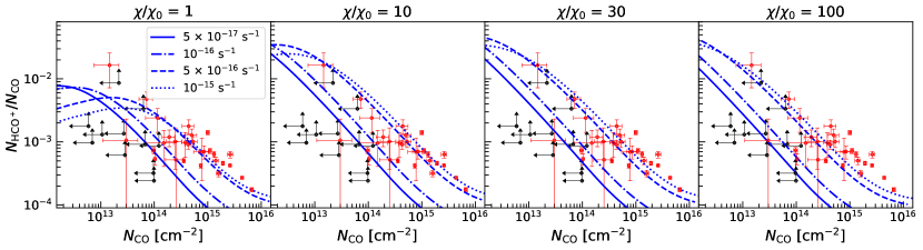
Figure 7: The observed relative abundance ratio (column density ratio) of $N_{\mathrm{HCO^{+}}}$/$N_{\mathrm{CO}}$ in Luo et al. (2020) overlaid on the predicted abundance ratios by PDR models with $n_{\rm H}$ = 10² cm^-3. From left to right represent the four representative FUV intensities ($\chi$/$\chi_{0}$ = 1, 10, 30, and 100). Red dots denote observations with both HCO⁺ and CO absorption detections. Black dots denote HCO⁺ absorptions without CO detection, it is thus a lower limit for $N_{\mathrm{HCO^{+}}}$/$N_{\mathrm{CO}}$. The four CRIR values used for modelling are 5$\times$10^-17, 10^-16, 5$\times$10^-16, and 10^-15 s^-1.

6.3 The CRIR inferred from HCO⁺ and CO absorptions

In order to quantitatively constrain $\zeta_{2}$ toward each source, we have run PDR models with ${\rm log_{10}\,(\zeta_{2}/s^{-1})}=-18$ to $-14$ with a step size of 0.07 dex and ${\rm log_{10}\,({\it n}_{\rm H}/cm^{-3})}$ = 1 – 3.5 with a step size of 0.1 dex, interacting with three FUV intensities ($\chi/\chi_{0}=1,5,10$). We vary $\zeta_{2}$ and $n_{\rm H}$ to find the optimum model by minimizing the reduced $\chi^{2}$ function:

$$\rm\chi^{2}_{red}=\frac{1}{N}\sum_{i}\frac{\left(f_{obs}^{i}-f_{model}^{i}\right)^{2}}{{\sigma^{i}_{obs}}^{2}},$$ (16)

where $\rm{f_{obs}^{i}}$ and ${\rm\sigma^{i}_{obs}}$ are the observed molecular column densities and their corresponding uncertainties of the $i$th species, respectively. $\rm{f_{model}^{i}}$ is the column density from PDR models and N = 1 is the degree of freedom.

We show two representative ${\rm\chi^{2}_{red}}$ distributions from our fitting in Figure 8. The higher values of ${\rm\chi^{2}_{red}}$ are colored with bright blue and the lower colored with dark blue. White color indicates values beyond the maximum in this colour-bar. Red contours represent the boundary of the best-fit parameter where the deviation between modeled values and observations is 1$\sigma$. We treat a fitting result with a minimal value of ${\rm\chi^{2}_{red}}\lesssim 1$ (upper panel of Figure 8) as a “high confidence” fit, and a fitting result with a minimal value of ${\rm\chi^{2}_{red}}\gg 1$ (lower panel of Figure 8) as a “low confidence” fit.

As seen from Figure 8, the best-fit values drift to both higher $\zeta_{2}$ and $n_{\rm H}$ as the increasing FUV intensity. However, at high FUV intensity, the best-fit value of $n_{\rm H}$ from PDR models is much higher than the allowable density range by MCMC runs (Table 1. On the other hand, increasing $\chi$/$\chi_{0}$ would increase $T_{\rm k}$. In that case, the inferred gas density should be lower (as seen in Figure 1). Thus, it is not likely that FUV intensity is high for our sources.

Here, we made a rough estimation of the FUV intensity in diffuse clouds. The interstellar radiation field is a function of dust temperature ($T_{\rm d}$, Beuther et al., 2014):

$$\chi/\chi_{0}=\frac{1}{1.7}\frac{4.7\times 10^{-31}}{5.6\times 10^{-26}}\frac{1}{\gamma(A_{\rm V})}T_{\rm d}^{6},$$ (17)

where $\gamma(A_{\rm V})$ is the attenuation factor. We consider $\gamma(A_{\rm V})$ = 0.35 at $A_{\rm V}$ = 1 mag (Glover & Clark, 2012). For $T_{\rm d}$ = 15 K, the derived FUV intensity is $\chi/\chi_{0}$ = 1.4. A variation on $T_{\rm d}$ of $\pm$2 K would only result in a difference on $\chi/\chi_{0}$ by a factor of 2. In the following, we only consider the fitting results at $\chi$/$\chi_{0}$ = 1.

Figure 8: The ${\rm\chi^{2}_{red}}$ distribution toward 3C454.3 V1 (up) and J0325+2224 (low) in the given parameter space. From left to right: ${\rm\chi^{2}_{red}}$ distribution at $\chi/\chi_{0}$ =1, 5, and 10. Red contours represent the boundary of where the deviation between modelled values and observations is 1$\sigma$.

The fitting results of all sources are summarised in Table 2, in which high confidence fit parameters are labelled with a “*” at the end of each row. The $\zeta_{2}$ in our sample (high confidence results) is in the range of $\zeta_{2}\sim 1.0_{-1.0}^{+14.8}$ $\times$10${}^{-16}-2.5_{-2.4}^{+1.4}$ $\times$10^-15 s^-1. The $n_{\rm H}$ is in the range of (0.1–3.2)$\times$10² cm^-3, which is consistent with that obtained from MCMC runs in Section 3.1.

In Fig. 9, we plot the Luo et al. (2023) $\zeta_{2}$ toward IC 348 measured from HCO⁺ and CO measurements, and the Indriolo & McCall (2012) $\zeta_{2}$ from H${}_{3}^{+}$ measurements. For comparison, we also include the Padovani et al. (2022) CR attenuation models $\mathscr{L}$, $\mathscr{H}$, and with low-energy spectral slope = $-$1.2. To plot $\zeta_{2}$ as a function of $E$(B-V), we convert N${}_{\rm H_{2}}$ to $E$(B-V) by assuming that the atomic fraction $f_{\rm atomic}$ follows the power law: $f_{\rm atomic}$ = 0.64/$A_{\rm V}$ at $A_{\rm V}>$1 mag (Luo et al., 2023), and the $f_{\rm atomic}$ = 0.64 at $A_{\rm V}\leq$1 mag. The average value of CRIR in our samples (red dots) is (8.0$\pm$6.4)$\times$10^-16 s^-1. This is $\sim 2$ times higher than the value measured with H${}^{+}_{3}$ toward nearby massive stars ($\zeta_{2}$ = 3.5${}^{+5.3}_{-3.0}$ $\times$10^-16 s^-1) and toward IC 348 (4.7$\pm$1.5 $\times$10^-16 s^-1, see Fig. 9). Considering that our sightlines are located at much lower $E$(B-V) (0.1 – 0.7 mag), the values are reasonably consistent with the low $E$(B-V) portion by Indriolo & McCall (2012). Our results are consistent with the model $\mathscr{H}$ by Padovani et al. (2018), in which CRs (and consequently the CRIR) are attenuated as a function of $A_{\rm V}$ (Padovani et al., 2018, 2022; Gaches et al., 2022). However, model $\mathscr{L}$, which corresponds to a “low” cosmic-ray spectrum based on Voyager-1 data, is found to underestimate the CRIR by almost an order of magnitude.

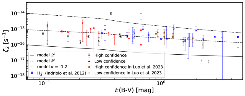
Figure 9: The red circles (high confidence fit) and black triangles (low confidence fit) show the inferred $\zeta_{2}$ in this work. Blue squares denote the measurements from H${}^{+}_{3}$ by Indriolo & McCall (2012). Brown crosses and gray stars are the high confidence fit and low confidence fit of $\zeta_{2}$ toward nearby star-forming cloud–IC 348. Black dashed, black solid, and black dash-dotted curves represent the polynomial fit to $\zeta_{2}$ at different $E$(B-V) for models $\mathscr{L}$, $\mathscr{H}$ and with low-energy spectral slope $\alpha$ = $-$1.2 by Padovani et al. (2022).

7 Conclusions

We analyze the abundances of CO, OH, and HCO⁺, and their abundance ratios in chemical equilibrium. We present a new approach to constrain the CRIR using these species. We calculated the column densities of HCO⁺ and CO toward diffuse LOSs against quasars and compare them with 3d-pdr models. Our inferred values of $\zeta_{2}$ show good consistency with previous measurements using H${}^{+}_{3}$. The main conclusions are as follows:

1. The gas volume densities ($n_{\rm H_{2}}$) obtained from CO (1–0) and (2–1) transitions toward 4 LOSs are in the range of (0.14$\pm$0.03 – 1.2$\pm$0.1)$\times$10² cm^-3 (at $T_{\rm k}$ = 50 K), which suggests a sub-thermal excitation environment for CO and HCO⁺.

2. Analyzing the chemical response of different molecules, we found that the abundance of CO increases with gas density and decreases with increasing FUV intensity, while the abundances of OH and HCO⁺ mostly have an opposite trend to that of CO.

3. Our analytic expressions give an excellent abundance of OH when $\zeta_{2}$ $<$10^-15 s^-1. This is potentially useful for hydrodynamical simulations as it reduces the computational expense of chemical networks. In the diffuse gas, the abundance of OH is proportional to the CRIR.

4. At a given $N_{\rm CO}$, the abundance ratio of OH/CO is monotonically increasing with the increase $\zeta_{2}$ in the diffuse cloud, while the abundance ratio of HCO⁺/CO increases reaching a local maximum value at $\zeta_{2}$ $\approx$ 10^-15 s^-1, before it decreases again. The downward trend of HCO⁺/CO at high $\zeta_{2}$ is caused due to the increased destruction of the precursor of HCO⁺–CO⁺ by electrons and atomic H at higher gas temperatures.

5. By comparing the observational values of HCO⁺/CO and chemical models, we find that the average $\zeta_{2}$ in our sample is (8.0$\pm$6.4)$\times$10^-15 s^-1. This value is $\sim$2 times higher than that of higher extinction regions, which is consistent with the hypothesis of decreasing $\zeta_{2}$ as the increasing $A_{\rm V}$ in theoretical studies.

With high-sensitivity measurements from HCO⁺ and CO, we have demonstrated the possibility of using HCO⁺/CO ratios to constrain the CRIR in diffuse gas without knowing the exact molecular abundances relative to H₂. We propose that the abundance ratios of OH/CO and HCO⁺/CO can be used to constrain the CRIR, especially with interferometry observations where high-resolution H₂ information is inaccessible. Due to the difficulties in obtaining accurate excitation and optical depth of OH with current facilities, we foresee that future instruments, such as SKA, will produce large samples of data sets for which our approach will be potentially useful.

Appendix A Derivation of abundance of OH in chemical equilibrium

The formation of OH is given by:

$$\rm F[{\it n}(OH)]= \ \rm{\it n}(H_{2}O^{+}){\it n}(e)k_{R6}$$

$$\ +\rm{\it n}(H_{2}O^{+}){\it n}(e)(k_{R9}+k_{R10})$$

$$\ +\rm{\it n}(H_{2}O)k_{pd}(R12),$$ (A1)

where $\rm{\it n}(H_{2}O^{+})$ can be written as:

$$\rm[{\it n}(H_{2}O^{+})]= \ \rm\frac{{\it n}(H_{2}O^{+}){\it n}(H_{2})k_{R5}}{{\it n}(e)(k_{R9}+k_{R10}+k_{R11})},$$ (A2)

and $\rm{\it n}(H_{2}O^{+})$ can be written as:

$$\rm[{\it n}(H_{2}O^{+})]= \ \rm\frac{{\it n}(OH^{+}){\it n}(H_{2})k_{R4}}{{\it n}(H_{2})k_{R5}+{\it n}(e)(k_{R6}+k_{R7}+k_{R8})}.$$ (A3)

The destruction of H₂O is dominated by photodissociation and C⁺ in the diffuse cloud (note that the destruction of H₂O will be dominated by H⁺ in dense cloud), thus, we have

$$\rm{\it n}(H_{2}O)= \ \rm\frac{{\it n}(H_{2}O^{+}){\it n}(e)k_{R11}}{k_{pd}(R12)+{\it n}(C^{+})k_{R13}}.$$ (A4)

Then, equation A1 can be written as:

$$\rm F[{\it n}(OH)]= \ \rm\frac{{\it n}(OH^{+}){\it n}(H_{2})k_{R4}}{{\it n}(H_{2})k_{R5}+{\it n}(e)(k_{R6}+k_{R7}+k_{R8})}$$

$$\ \times\rm[{\it n}(e)k_{R6}+{\it n}(H_{2})k_{R5}(1-\delta)],$$ (A5)

where $\delta$ is:

$$\rm\delta= \ \rm\frac{k_{R11}}{k_{R9}+k_{R10}+k_{R11}}\times$$

$$\ \rm\frac{{\it n}(C^{+})k_{R13}}{k_{pd}(R12)+{\it n}(C^{+})k_{R13}}.$$ (A6)

Considering chemical equilibrium of $\rm{\it n}(OH^{+})$, the term $\rm{\it n}(OH^{+}){\it n}(H_{2})k_{R4}$ can be written as:

$$\rm{\it n}(OH^{+}){\it n}(H_{2})k_{R4}= \ \rm{\it n}(O^{+}){\it n}(H_{2})k_{R2}+{\it n}(O){\it n}(H_{3}^{+})k_{R3}$$

$$= \ \rm{\it n}(O)[{\it n}(H^{+})k_{R1}+\zeta_{O}+{\it n}(H_{3}^{+})k_{R3}],$$ (A7)

where $\zeta_{\rm O}$ $\approx$ 2.83$\zeta_{2}$ is the cosmic-ray ionization rate of atomic oxygen.

H⁺ is produced by cosmic-rays (CRs):

$$\rm H+CRs\rightarrow \ \rm H^{+}+e,$$ (RA1)

$$\rm H_{2}+CRs\rightarrow \ \rm H^{+}+H+e,$$ (RA2)

$$\rm H_{2}^{+}+H\rightarrow \ \rm H_{2}+H^{+},$$ (RA3)

and removed by atomic oxygen (reaction R1) and electron recombination reaction:

$$\rm H^{+}+e\rightarrow H+h\nu.$$ (RA4)

In chemical equilibrium, $\rm{{\it n}(H^{+})}$ is in the form of:

$$\rm{\it n}(H^{+})= \ \rm\frac{{\it n}(HI)k_{RA1}+{\it n}(H_{2})k_{RA2}+{\it n}(H_{2}^{+})k_{RA3}}{{\it n}(e)k_{RA4}+{\it n}(O)k_{R1}},$$ (A8)

in which H${}_{2}^{+}$ is formed through:

$$\rm H_{2}+CRs\rightarrow \ \rm H_{2}^{+}+e,$$ (RA5)

and removed by H through reaction RA3 or by H₂ through:

$$\rm H_{2}^{+}+H_{2}\rightarrow H_{3}^{+}+H.$$ (RA6)

Thus, equation A8 can be written as:

$$\rm{\it n}(H^{+})= \ \rm\frac{{\it n}(HI)k_{RA1}+{\it n}(H_{2})k_{RA2}+{\it n}(H_{2})k_{RA5}\xi}{{\it n}(e)k_{RA4}+{\it n}(O)k_{R1}},$$ (A9)

where $\rm{k_{RA1}}$ = $\zeta_{1}$ = 1/2$\zeta_{2}$, $\rm{k_{RA2}}$ = 0.02 $\zeta_{2}$, $\rm{k_{RA5}}$ = 0.88 $\zeta_{2}$, and $\xi$ is in the form of:

$$\rm\xi= \ \rm\frac{{\it n}(HI)k_{RA3}}{{\it n}(HI)k_{RA3}+{\it n}(H_{2})k_{RA6}}$$

$$= \ \rm\frac{2-2{\it f}_{mol}}{2+1.25{\it f}_{mol}}.$$ (A10)

Thus, if $\rm{{\it f}_{mol}}$ is close to 1, $\xi$=0. Otherwise, if $\rm{{\it f}_{mol}}$ is close to 0, $\xi$=1.

However, equation A9 does not consider the formation of H⁺ by He⁺. The formation of He⁺ is mainly due to the He ionization due to CRs:

$$\rm He+CRs\rightarrow \ \rm He^{+}+e.$$ (RA7)

The destruction of He⁺ is either dominated by H or H₂ in diffuse cloud:

$$\rm He^{+}+H\rightarrow H^{+}+He,$$ (RA8)

$$\rm He^{+}+H_{2}\rightarrow H^{+}+H+He,$$ (RA9)

$$\rm He^{+}+H_{2}\rightarrow H_{2}^{+}+He.$$ (RA10)

In equilibrium, n(He⁺) can be written as:

$$\rm n(He^{+})= \ \rm\frac{{\it n}(He)k_{RA7}}{{\it n}(HI)k_{RA8}+{\it n}(H_{2})(k_{RA9}+k_{RA10})},$$ (A11)

where $\rm{k_{RA7}}$ = 0.5 $\zeta_{2}$.

If we take reactions RA8 and RA9 into account, equation A9 can be rewritten as:

$$\ \rm{\it n}(H^{+})=$$

$$\ \rm\frac{{\it n}(HI)k_{RA1}+{\it n}(H_{2})k_{RA2}+{\it n}(H_{2})k_{RA5}\xi+{\it n}(He)k_{RA7}}{{\it n}(e)k_{RA4}+{\it n}(O)k_{R1}}$$

$$= \ \rm\frac{{\it n}(HI)k_{RA1}+{\it n}(H_{2})k_{RA2}+{\it n}(H_{2})k_{RA5}\xi+0.1{\it n}(H)k_{RA7}}{{\it n}(e)k_{RA4}+{\it n}(O)k_{R1}}$$

$$= \ \rm\frac{0.5[1.1-(0.98-0.88\xi){\it f}_{mol}]{\it n}(H)\zeta_{2}}{{\it n}(e)k_{RA4}+{\it n}(O)k_{R1}}.$$ (A12)

H${}_{3}^{+}$ is formed through reaction RA6 and removed by electrons:

$$\rm H_{3}^{+}+e\rightarrow \ \rm H_{2}+H,$$ (RA11)

$$\rm\rightarrow \ \rm H+H+H.$$ (RA12)

Thus, $\rm{{\it n}(H_{3}^{+})}$ is in the form of:

$$\rm{\it n}(H_{3}^{+})= \ \rm\frac{{\it n}(H_{2})^{2}k_{RA5}k_{RA6}}{{\it n}(e)(k_{RA11}+k_{RA12})[{\it n}(HI)k_{RA3}+{\it n}(H_{2})k_{RA6}]}.$$ (A13)

Note that equation A13 does not consider the destruction of H${}^{+}_{3}$ by CO and O (see also equation 18 in Indriolo & McCall (2012)), however, equation A13 is a good approximation in diffuse and translucent clouds since the destruction rate by electrons is more than two orders of magnitude higher than that of CO or O.

If we substitute equation A7 with equation A9 and A13, we have:

$$\ \rm{\it n}(OH^{+}){\it n}(H_{2})k_{R4}$$

$$= \ \rm{\it n}(O)\zeta_{2}[\frac{0.5(1.1-(0.98-0.88\xi){\it f}_{mol})k_{R1}{\it n}(H)}{{\it n}(e)k_{RA4}+{\it n}(O)k_{R1}}$$

$$\ \rm+2.83+\frac{0.22{\it f}_{mol}^{2}k_{RA6}k_{R3}{\it n}(H)}{{\it n}(e)(k_{RA11}+k_{RA12})}\times$$

$$\ \rm\frac{1}{(1-{\it f}_{mol})k_{RA3}+0.5{\it f}_{mol}k_{RA6}}]$$

$$= \ \rm{\it n}(O)\zeta_{2}\theta,$$ (A14)

where $\theta$ is in the form of:

$$\theta= \ \rm\frac{0.5(1.1-(0.98-0.88\xi){\it f}_{mol})k_{R1}{\it n}(H)}{{\it n}(e)k_{RA4}+{\it n}(O)k_{R1}}$$

$$\ \rm+2.83+\frac{0.22{\it f}_{mol}^{2}k_{RA6}k_{R3}{\it n}(H)}{{\it n}(e)(k_{RA11}+k_{RA12})}\times$$

$$\ \rm\frac{1}{(1-{\it f}_{mol})k_{RA3}+0.5{\it f}_{mol}k_{RA6}},$$ (A15)

which denotes the last term in equation A14. Combining equations A5 and A14, we thus obtain:

$$\rm F[{\it n}(OH)]= \ \rm{\it n}(O)\zeta_{2}\theta\times$$

$$\ \rm\frac{{\it n}(e)k_{R6}+{\it n}(H_{2})k_{R5}(1-\delta)}{{\it n}(H_{2})k_{R5}+{\it n}(e)(k_{R6}+k_{R7}+k_{R8})}$$

$$= \ \rm{\it n}(O)\zeta_{2}\theta\times$$

$$\ \rm[1-\frac{{\it n}(H_{2})k_{R5}\delta+{\it n}(e)(k_{R7}+k_{R8})}{{\it n}(H_{2})k_{R5}+{\it n}(e)(k_{R6}+k_{R7}+k_{R8})}].$$ (A16)

The destruction of OH is given by:

$$\rm D[{\it n}(OH)]= \ \rm{\it n}(OH)k_{pd}(R14)$$

$$\ \rm+{\it n}(OH){\it n}(C^{+})(k_{R15}+k_{R16})$$

$$\ \rm+{\it n}(OH){\it n}(H^{+})k_{R17}.$$ (A17)

In equilibrium, the formation and destruction of OH reach a balance ($\rm F[{\it n}(OH)]$ = $\rm D[{\it n}(OH)]$).

References

- Astropy Collaboration et al. (2013) Astropy Collaboration, Robitaille, T. P., Tollerud, E. J., et al. 2013, A&A, 558, A33, doi: 10.1051/0004-6361/201322068
- Astropy Collaboration et al. (2018) Astropy Collaboration, Price-Whelan, A. M., Sipőcz, B. M., et al. 2018, AJ, 156, 123, doi: 10.3847/1538-3881/aabc4f
- Bacalla et al. (2019) Bacalla, X. L., Linnartz, H., Cox, N. L. J., et al. 2019, A&A, 622, A31, doi: 10.1051/0004-6361/201833039
- Beuther et al. (2014) Beuther, H., Ragan, S. E., Ossenkopf, V., et al. 2014, A&A, 571, A53, doi: 10.1051/0004-6361/201424757
- Bialy et al. (2019) Bialy, S., Neufeld, D., Wolfire, M., Sternberg, A., & Burkhart, B. 2019, ApJ, 885, 109, doi: 10.3847/1538-4357/ab487b
- Bisbas et al. (2012) Bisbas, T. G., Bell, T. A., Viti, S., Yates, J., & Barlow, M. J. 2012, MNRAS, 427, 2100, doi: 10.1111/j.1365-2966.2012.22077.x
- Bisbas et al. (2017) Bisbas, T. G., van Dishoeck, E. F., Papadopoulos, P. P., et al. 2017, ApJ, 839, 90, doi: 10.3847/1538-4357/aa696d
- Burgh et al. (2007) Burgh, E. B., France, K., & McCandliss, S. R. 2007, ApJ, 658, 446, doi: 10.1086/511259
- Busch et al. (2021) Busch, M. P., Engelke, P. D., Allen, R. J., & Hogg, D. E. 2021, ApJ, 914, 72, doi: 10.3847/1538-4357/abf832
- Caselli et al. (1998) Caselli, P., Walmsley, C. M., Terzieva, R., & Herbst, E. 1998, ApJ, 499, 234, doi: 10.1086/305624
- Cotten et al. (2012) Cotten, D. L., Magnani, L., Wennerstrom, E. A., Douglas, K. A., & Onello, J. S. 2012, AJ, 144, 163, doi: 10.1088/0004-6256/144/6/163
- Crutcher (1979) Crutcher, R. M. 1979, ApJ, 234, 881, doi: 10.1086/157570
- Dalgarno (2006) Dalgarno, A. 2006, Proceedings of the National Academy of Science, 103, 12269, doi: 10.1073/pnas.0602117103
- Draine (1978) Draine, B. T. 1978, ApJS, 36, 595, doi: 10.1086/190513
- Foreman-Mackey et al. (2013) Foreman-Mackey, D., Hogg, D. W., Lang, D., & Goodman, J. 2013, PASP, 125, 306, doi: 10.1086/670067
- Frerking et al. (1982) Frerking, M. A., Langer, W. D., & Wilson, R. W. 1982, ApJ, 262, 590, doi: 10.1086/160451
- Gaches et al. (2022) Gaches, B. A. L., Bisbas, T. G., & Bialy, S. 2022, A&A, 658, A151, doi: 10.1051/0004-6361/202142411
- Geballe et al. (1999) Geballe, T. R., McCall, B. J., Hinkle, K. H., & Oka, T. 1999, ApJ, 510, 251, doi: 10.1086/306580
- Gerin et al. (2019) Gerin, M., Liszt, H., Neufeld, D., et al. 2019, A&A, 622, A26, doi: 10.1051/0004-6361/201833661
- Gerin et al. (2010) Gerin, M., de Luca, M., Black, J., et al. 2010, A&A, 518, L110, doi: 10.1051/0004-6361/201014576
- Glover & Clark (2012) Glover, S. C. O., & Clark, P. C. 2012, MNRAS, 421, 116, doi: 10.1111/j.1365-2966.2011.20260.x
- Godard et al. (2010) Godard, B., Falgarone, E., Gerin, M., Hily-Blant, P., & de Luca, M. 2010, A&A, 520, A20, doi: 10.1051/0004-6361/201014283
- Goldsmith (2001) Goldsmith, P. F. 2001, ApJ, 557, 736, doi: 10.1086/322255
- Goldsmith (2013) —. 2013, ApJ, 774, 134, doi: 10.1088/0004-637X/774/2/134
- Goldsmith et al. (2008) Goldsmith, P. F., Heyer, M., Narayanan, G., et al. 2008, ApJ, 680, 428, doi: 10.1086/587166
- Green et al. (2019) Green, G. M., Schlafly, E., Zucker, C., Speagle, J. S., & Finkbeiner, D. 2019, ApJ, 887, 93, doi: 10.3847/1538-4357/ab5362
- Grenier et al. (2015) Grenier, I. A., Black, J. H., & Strong, A. W. 2015, ARA&A, 53, 199, doi: 10.1146/annurev-astro-082214-122457
- Guelin et al. (1982) Guelin, M., Langer, W. D., & Wilson, R. W. 1982, A&A, 107, 107
- Indriolo et al. (2010) Indriolo, N., Blake, G. A., Goto, M., et al. 2010, ApJ, 724, 1357, doi: 10.1088/0004-637X/724/2/1357
- Indriolo & McCall (2012) Indriolo, N., & McCall, B. J. 2012, ApJ, 745, 91, doi: 10.1088/0004-637X/745/1/91
- Indriolo et al. (2015) Indriolo, N., Neufeld, D. A., Gerin, M., et al. 2015, ApJ, 800, 40, doi: 10.1088/0004-637X/800/1/40
- Le Petit et al. (2016a) Le Petit, F., Ruaud, M., Bron, E., et al. 2016a, A&A, 585, A105, doi: 10.1051/0004-6361/201526658
- Le Petit et al. (2016b) —. 2016b, A&A, 585, A105, doi: 10.1051/0004-6361/201526658
- Li et al. (2018) Li, D., Tang, N., Nguyen, H., et al. 2018, ApJS, 235, 1, doi: 10.3847/1538-4365/aaa762
- Liszt & Gerin (2018) Liszt, H., & Gerin, M. 2018, A&A, 610, A49, doi: 10.1051/0004-6361/201731983
- Liszt & Gerin (2023) —. 2023, arXiv e-prints, arXiv:2301.08945, doi: 10.48550/arXiv.2301.08945
- Liszt & Lucas (1996) Liszt, H., & Lucas, R. 1996, A&A, 314, 917
- Liszt & Lucas (2000) —. 2000, A&A, 355, 333
- Liszt & Lucas (2002) —. 2002, A&A, 391, 693, doi: 10.1051/0004-6361:20020849
- Liszt (2007) Liszt, H. S. 2007, A&A, 476, 291, doi: 10.1051/0004-6361:20078502
- Liszt & Gerin (2016) Liszt, H. S., & Gerin, M. 2016, A&A, 585, A80, doi: 10.1051/0004-6361/201527273
- Liszt & Lucas (1998) Liszt, H. S., & Lucas, R. 1998, A&A, 339, 561
- Lucas & Liszt (1996) Lucas, R., & Liszt, H. 1996, A&A, 307, 237
- Luo et al. (2020) Luo, G., Li, D., Tang, N., et al. 2020, ApJ, 889, L4, doi: 10.3847/2041-8213/ab6337
- Luo et al. (2023) Luo, G., Zhang, Z.-Y., Bisbas, T. G., et al. 2023, ApJ, 942, 101, doi: 10.3847/1538-4357/aca657
- Magnani et al. (1988) Magnani, L., Blitz, L., & Wouterloot, J. G. A. 1988, ApJ, 326, 909, doi: 10.1086/166149
- Mangum & Shirley (2015) Mangum, J. G., & Shirley, Y. L. 2015, PASP, 127, 266, doi: 10.1086/680323
- McCall et al. (1999) McCall, B. J., Geballe, T. R., Hinkle, K. H., & Oka, T. 1999, ApJ, 522, 338, doi: 10.1086/307637
- McClure-Griffiths et al. (2015) McClure-Griffiths, N. M., Stanimirovic, S., Murray, C., et al. 2015, in Advancing Astrophysics with the Square Kilometre Array (AASKA14), 130, doi: 10.22323/1.215.0130
- McDowell (1987) McDowell, R. S. 1987, J. Quant. Spec. Radiat. Transf., 38, 337, doi: 10.1016/0022-4073(87)90028-8
- McElroy et al. (2013) McElroy, D., Walsh, C., Markwick, A. J., et al. 2013, A&A, 550, A36, doi: 10.1051/0004-6361/201220465
- McMullin et al. (2007) McMullin, J. P., Waters, B., Schiebel, D., Young, W., & Golap, K. 2007, in Astronomical Society of the Pacific Conference Series, Vol. 376, Astronomical Data Analysis Software and Systems XVI, ed. R. A. Shaw, F. Hill, & D. J. Bell, 127
- Müller et al. (2005) Müller, H. S. P., Schlöder, F., Stutzki, J., & Winnewisser, G. 2005, Journal of Molecular Structure, 742, 215, doi: 10.1016/j.molstruc.2005.01.027
- Müller et al. (2001) Müller, H. S. P., Thorwirth, S., Roth, D. A., & Winnewisser, G. 2001, A&A, 370, L49, doi: 10.1051/0004-6361:20010367
- Neufeld & Wolfire (2017) Neufeld, D. A., & Wolfire, M. G. 2017, ApJ, 845, 163, doi: 10.3847/1538-4357/aa6d68
- Oka et al. (2005) Oka, T., Geballe, T. R., Goto, M., Usuda, T., & McCall, B. J. 2005, ApJ, 632, 882, doi: 10.1086/432679
- Padovani et al. (2013) Padovani, M., Hennebelle, P., & Galli, D. 2013, A&A, 560, A114, doi: 10.1051/0004-6361/201322407
- Padovani et al. (2018) Padovani, M., Ivlev, A. V., Galli, D., & Caselli, P. 2018, A&A, 614, A111, doi: 10.1051/0004-6361/201732202
- Padovani et al. (2020) Padovani, M., Ivlev, A. V., Galli, D., et al. 2020, Space Sci. Rev., 216, 29, doi: 10.1007/s11214-020-00654-1
- Padovani et al. (2022) Padovani, M., Bialy, S., Galli, D., et al. 2022, A&A, 658, A189, doi: 10.1051/0004-6361/202142560
- Pety et al. (2017) Pety, J., Guzmán, V. V., Orkisz, J. H., et al. 2017, A&A, 599, A98, doi: 10.1051/0004-6361/201629862
- Pineda et al. (2010) Pineda, J. L., Goldsmith, P. F., Chapman, N., et al. 2010, ApJ, 721, 686, doi: 10.1088/0004-637X/721/1/686
- Röllig et al. (2007) Röllig, M., Abel, N. P., Bell, T., et al. 2007, A&A, 467, 187, doi: 10.1051/0004-6361:20065918
- Schlafly & Finkbeiner (2011) Schlafly, E. F., & Finkbeiner, D. P. 2011, ApJ, 737, 103, doi: 10.1088/0004-637X/737/2/103
- Sheffer et al. (2008) Sheffer, Y., Rogers, M., Federman, S. R., et al. 2008, ApJ, 687, 1075, doi: 10.1086/591484
- Spitzer & Tomasko (1968) Spitzer, Lyman, J., & Tomasko, M. G. 1968, ApJ, 152, 971, doi: 10.1086/149610
- Strong et al. (2007) Strong, A. W., Moskalenko, I. V., & Ptuskin, V. S. 2007, Annual Review of Nuclear and Particle Science, 57, 285, doi: 10.1146/annurev.nucl.57.090506.123011
- Tang et al. (2021) Tang, N., Li, D., Yue, N., et al. 2021, ApJS, 252, 1, doi: 10.3847/1538-4365/abca94
- Turner (1979) Turner, B. E. 1979, A&AS, 37, 1
- van der Tak et al. (2007) van der Tak, F. F. S., Black, J. H., Schöier, F. L., Jansen, D. J., & van Dishoeck, E. F. 2007, A&A, 468, 627, doi: 10.1051/0004-6361:20066820
- van der Tak & van Dishoeck (2000) van der Tak, F. F. S., & van Dishoeck, E. F. 2000, A&A, 358, L79. https://arxiv.org/abs/astro-ph/0006246
- Vaupré et al. (2014) Vaupré, S., Hily-Blant, P., Ceccarelli, C., et al. 2014, A&A, 568, A50, doi: 10.1051/0004-6361/201424036
- Wannier et al. (1993) Wannier, P. G., Andersson, B. G., Federman, S. R., et al. 1993, ApJ, 407, 163, doi: 10.1086/172502
- Webber (1998) Webber, W. R. 1998, ApJ, 506, 329, doi: 10.1086/306222
- Xu & Li (2016) Xu, D., & Li, D. 2016, ApJ, 833, 90, doi: 10.3847/1538-4357/833/1/90
- Xu et al. (2016) Xu, D., Li, D., Yue, N., & Goldsmith, P. F. 2016, ApJ, 819, 22, doi: 10.3847/0004-637X/819/1/22
- Zhou et al. (2022) Zhou, P., Zhang, G.-Y., Zhou, X., et al. 2022, ApJ, 931, 144, doi: 10.3847/1538-4357/ac63b5