autofz: Automated Fuzzer Composition at Runtime

Abstract

Fuzzing has gained in popularity for software vulnerability detection by virtue of the tremendous effort to develop a diverse set of fuzzers. Thanks to various fuzzing techniques, most of the fuzzers have been able to demonstrate great performance on their selected targets. However, paradoxically, this diversity in fuzzers also made it difficult to select fuzzers that are best suitable for complex real-world programs, which we call selection burden. Communities attempted to address this problem by creating a set of standard benchmarks to compare and contrast the performance of fuzzers for a wide range of applications, but the result was always a suboptimal decision—the best performing fuzzer on average does not guarantee the best outcome for the target of a user’s interest.

To overcome this problem, we propose an automated, yet non-intrusive meta-fuzzer, called autofz , to maximize the benefits of existing state-of-the-art fuzzers via dynamic composition. To an end user, this means that, instead of spending time on selecting which fuzzer to adopt (similar in concept to hyperparameter tuning in ML), one can simply put all of the available fuzzers to autofz (similar in concept to AutoML), and achieve the best, optimal result. The key idea is to monitor the runtime progress of the fuzzers, called trends (similar in concept to gradient descent), and make a fine-grained adjustment of resource allocation (e.g., CPU time) of each fuzzer. This is a stark contrast to existing approaches that statically combine a set of fuzzers, or via exhaustive pre-training per target program—autofz deduces a suitable set of fuzzers of the active workload in a fine-grained manner at runtime. Our evaluation shows that, given the same amount of computation resources, autofz outperforms any best-performing individual fuzzers in 11 out of 12 available benchmarks and beats the best, collaborative fuzzing approaches in 19 out of 20 benchmarks without any prior knowledge in terms of coverage. Moreover, on average, autofz found 152% more bugs than individual fuzzers on UniFuzz and FTS, and 415% more bugs than collaborative fuzzing on UniFuzz.

1 Introduction

Complications in modern programs inevitably entangle the manual analysis of software and further reduce the chance of discovering software defects. To overcome this, researchers and industry have conducted extensive studies on discovering software vulnerabilities with automation, called fuzzing [35, 4, 32]. Fuzzing generates input expected to trigger the defects in the program with feedback retrieved from multiple rounds of execution and monitors for any anomalies. To enhance the performance of fuzzing, a great deal of research using different techniques has been proposed [42, 50, 9, 8, 40, 25, 26, 6, 48, 43, 51, 47, 38, 28, 49, 17, 3, 31, 24, 1, 5]. As a result, fuzzing has demonstrated its effectiveness in disclosing vulnerabilities from off-the-shelf binaries [14, 39, 51, 44, 20]. Motivated by convincing empirical evidence for the practicality of fuzzing, Google [19, 18] and, recently, Microsoft [34] have deployed scalable fuzzers.

Figure 1: Performance of autofz and baseline fuzzers presented with coverage ratio of fuzzing exiv2 and ffmpeg during 24 hours. Each graph is generated with an arithmetic mean and 80% confidence interval for 10 fuzzing rounds. Coverage ratio is a percentage of branches explored by each fuzzer. We carefully selected two test suites from Figure 3 to highlight the motivation of autofz.

However, the remarkable enhancement and diversity of fuzzers create a selection burden, paradoxically, that requires another significant engineering effort to select the best-performing fuzzer(s) per target (similar in concept to hyperparameter tuning). Note that fuzzer selection is a dominant factor that contributes to vulnerability detection and its efficiency. As shown in Figure 1, the outcome significantly varies depending on which fuzzer is selected. For example, with the same amount of resources, Redqueen outperforms Radamsa by more than 10 times in fuzzing exiv2 (left graph).

A handful of research efforts have tried to mitigate the selection problem [27]. Fuzzing benchmarks [12, 21, 33, 15, 23, 29, 36] enumerate well-suited fuzzers for each benchmark target. The evaluation of the benchmark helps users to understand which fuzzers are favorable for fuzzing different types of binaries. Recently, collaborative fuzzing [10, 22, 53] has showcased that cooperating different combinations of fuzzers sometimes outperforms individual fuzzers thanks to their corpus sharing. However, this still imposes the burden of selecting what fuzzers to put into an ensemble. Moreover, the selection of fuzzers generally requires significant computing and human resources because it relies on static information.

Unlike previous works, autofz automatically deploys a set of fuzzer(s) per workload, not per program. The goal of autofz is to completely automate the selection problem via the dynamic composition of fuzzers as a push-button solution. Therefore, when end users select a set of baseline fuzzers, autofz automatically devises the best performance utilizing runtime information.

autofz is largely motivated by the following observations:

1) No universal fuzzer invariably outperforms others..1) No universal fuzzer invariably outperforms others.1) No universal fuzzer invariably outperforms others.. As shown in  Figure 1, a particular fuzzer cannot persistently achieve optimal performance independent of the workload. For example, LearnAFL is demonstrated to be the best-performing fuzzer for fuzzing the ffmpeg binary. However, when the target is changed to exiv2, LearnAFL is relegated to sixth place, which shows the lack of consistency in the performance of fuzzers against different binaries. Unfortunately, this inconsistency is not uncommon [29, 33]. Therefore, to achieve better performance, significant engineering effort is required to handpick the fuzzers whenever the target binary is changed or a new fuzzer is introduced.

2) The efficiency of each fuzzer is not perpetual throughout..2) The efficiency of each fuzzer is not perpetual throughout.2) The efficiency of each fuzzer is not perpetual throughout.. As shown in Figure 1, initially, Angora significantly outperforms the others in fuzzing the exiv2 binary. However, LAF-Intel and Redqueen come from behind and take the lead after about two hours. We call this rank inversion. Note that another inversion occurs after 12 hours have elapsed. LAF-Intel initially slightly outperforms Redqueen, but Redqueen becomes the best in the end result. Moreover, we found that rank inversion occurs more frequently when seed synchronization is introduced to share the interesting input among multiple fuzzers (§ 6.8). This result indicates that sticking to the initially chosen fuzzer during the entire execution cannot achieve optimal performance.

3) Naive resource allocation results in inefficiency..3) Naive resource allocation results in inefficiency.3) Naive resource allocation results in inefficiency.. Unfortunately, all collaborative fuzzing approaches have focused only on selecting the best combination of fuzzers and running the fuzzers assigned with equally partitioned resources. However, in addition to fuzzer selection, the resource distribution among the selected fuzzers can severely affect the performance of fuzzing. To achieve better results, the performance of each fuzzer should be assessed and considered to distribute resources among the selected fuzzers.

4) Randomness in fuzzing prevents reproductions.4) Randomness in fuzzing prevents reproductions4) Randomness in fuzzing prevents reproductions. More important, note that this trend will not invariably be captured in different fuzzing executions because fuzzing is inherently a random process. Therefore, even though experts put a lot of effort into locating the best combinations of fuzzers and associated guidance information such as appropriate time to switch fuzzers and resource allocation, this statically analyzed information may not be consistent across subsequent fuzzing runs, even for the same target binary. Consequently, statically prearranging those configurations might result in losing the benefits of promptly dealing with a different workload with most suitable fuzzers.

2 Our Approach: Using Trend Per Workload

Given the aforementioned challenges, timely locating the best performing fuzzer(s) is non-trivial, as the workload changes during the fuzzing execution. In this paper, we propose autofz, an automated meta-fuzzer that outperforms the best individual fuzzers in any target without implementing any particular fuzzing algorithm. The key idea of autofz is to dynamically deploy a set of, or possibly all, of fuzzers along with efficient utilization guidance, such as resource allocation, per workload, not per program. We call the runtime progress of baseline fuzzers a trend. Specifically, autofz switches fuzzers and adjusts resources as the trend changes, instead of adhering to a particular set of fuzzers, during an entire execution.

autofz splits its execution into two different phases, preparation and focus phases (Figure 2), to monitor the trend changes. The preparation phase captures the runtime trend of target binaries and deploys fuzzers that illustrate strong trends. Based on the captured trend and the guidance information, the focus phase tries to achieve the optimal performance with the selected fuzzers. Also, the dynamic resource adjustment of autofz utilizing guidance information allows it to enjoy the best of both an individual fuzzer and a combination of different fuzzers. On the one hand, it can prioritize a particular fuzzer, significantly outperforming others by allocating all resources to the selected fuzzer. On the other hand, autofz takes advantage of multiple fuzzers by distributing resources.

More important, unlike previous approaches that utilize benchmark and offline analysis to select well-suited fuzzers beforehand, autofz does not require significant engineering effort or hindsight because it dynamically adopts the trends and automatically configures the best fuzzer set at runtime. Therefore, autofz can devote additional resources that were previously spent on offline analysis to the actual fuzzing campaign. Moreover, such an approach bridges the gap between developing a fuzzer and its utilization and provides unprecedented opportunities. For example, even non-expert users, without any knowledge about the selected fuzzers and target binaries, can achieve better fuzzing performance on any target program. Furthermore, we integrate autofz into Fuzzer Test Suite and UniFuzz, which support the most efficient and widely used fuzzers. Therefore, autofz can readily benefit from any fuzzer that will be integrated into those benchmarks.

We evaluate autofz on Fuzzer Test Suite and UniFuzz to demonstrate how autofz can efficiently utilize multiple different fuzzers. Our evaluation demonstrates that autofz can significantly outperform most of the individual fuzzers supported by the benchmarks regardless of the target binaries. Moreover, we expand autofz to support a multi-core environment and compare it with collaborative fuzzing, such as EnFuzz and Cupid. We found that the resource allocation strategy and fine-grained fuzzer scheduling of autofz help it to achieve better performance in most of the target binaries.

This paper makes the following main contributions:

• A dynamic fuzzer composition per workload..A dynamic fuzzer composition per workload.A dynamic fuzzer composition per workload.. Existing approaches aim to find a static group of fuzzers that work best for each target program. However, careful consideration of per-workload dynamic trends allows autofz to avoid benchmark-based decisions biased to a specific target program. Therefore, autofz does not need to utilize one static group of fuzzers during the entire fuzzing campaign. In essence, as well as consistently selecting well-performing fuzzers, autofz can give a second chance to fuzzers that have not been selected but turn out to be suitable for a particular workload later.

• Automatic and non-intrusive approach..Automatic and non-intrusive approach.Automatic and non-intrusive approach.. For end users, autofz is a push-button solution that automatically selects the best suitable fuzzers for any given target. For fuzzer developers, each fuzzer can be integrated to autofz with minimal engineering effort: 126 LoC changes on average are required in the 11 fuzzers we support initially (§ 5). We call autofz a meta-fuzzer because it implements no fuzzing algorithm internally.

• Efficient resource scheduling algorithm..Efficient resource scheduling algorithm.Efficient resource scheduling algorithm.. autofz measures the performance of individual fuzzers and efficiently distributes computational resources to the selected fuzzers. This helps autofz take advantage of the strong trend of individual fuzzers while maximizing the collaboration effects of multiple different fuzzers. Moreover, autofz first highlights the resource scheduling as another important factor affecting the efficiency of the collaboration. The collaboration effect can be maximized when the resources are properly assigned among the selected fuzzers.

3 Related work

Fuzzing benchmark.Fuzzing benchmarkFuzzing benchmark. The lack of metrics and representative target programs in fuzzing research prevents their results from being reproducible, making it difficult for users to decide which fuzzers are suitable for fuzzing specific target programs. To mitigate this problem and provide a standardized test suite for various fuzzers, several fuzzing benchmarks have been proposed. LAVA-M [15] provides a set of benchmark programs that contain syntactically injected out-of-bounds memory access vulnerabilities. The Cyber Grand Challenge [12] benchmark consists of various target binaries having a wide variety of synthetic software defects. Fuzzer Test Suite (FTS) [21] evaluates fuzzers against real-world vulnerabilities. FuzzBench [33] improved FTS and provide the frontend interface that allows smooth integration of new benchmarks and fuzzers. Moreover, UniFuzz [29] and Magma [23] provide benchmarks that have real-world vulnerabilities together with their ground truth to verify genuine software defects from random software crashes.

Collaborative fuzzing..Collaborative fuzzing.Collaborative fuzzing.. Collaborative fuzzing attempts to improve the performance of a fuzzing campaign by orchestrating multiple different types of fuzzers with seed synchronization (see below). EnFuzz [10] first demonstrated that deploying various types of fuzzers together allows it to achieve better code coverage. Recently, Cupid [22] showcased that offline analysis with a training set, including empirically collected representative branches, is able to predict target-independent fuzzer combinations. In addition to fuzzer selection, CollabFuzz [53] illustrates the importance of test case scheduling policies in seed synchronization among the selected fuzzers.

	EnFuzz	Cupid	autofz
Number of selected fuzzers	user-configured	user-configured	automatic
	(2-4)	(2-4)	(1-11)
Fuzzer switches at runtime?	✗	✗	✓
Require prior knowledge?	✓	✓	✗
Cost of pre-training	low	high	none
Target-independent decision?	✗	▲	✓
Cost of adding new fuzzers?	✓	✓	✗
Resource allocation	static	static	dynamic
Resource distribution policy	equal	equal	proportional

Table 1: Comparison of EnFuzz, Cupid, and autofz.

Table 1 provides comparisons between autofz and collaborative fuzzing. The most noticeable difference is that autofz utilizes the runtime information in the fuzzer selection and resource adjustment, which results in subsequent differences.

Seed synchronization.Seed synchronizationSeed synchronization. Seed synchronization [18, 51, 30] allows the sharing of interesting seeds generated by different instances of the same fuzzer. Moreover, it helps various modern fuzzers utilize multi-core processors [51, 6, 31, 28, 49, 9, 3]. It has been extended by [10, 53] to share unique test cases produced by different fuzzers. In essence, seed synchronization introduces interesting inputs borrowed from other fuzzers to a particular fuzzer that consistently fails to make progress.

AFL bitmap. Various numbers of fuzzers adopt AFL bitmap to measure the performance of their fuzzing techniques [51, 6, 7, 31, 28, 49, 1]. Recently, Angora [9] and AFL-Sensitive [45] adopted AFL bitmap in addition to call contexts to implement a context-sensitive bitmap. In essence, AFL bitmap records the path explored during a fuzzing campaign, measuring code coverage [52]. Also, the bitmap can be utilized as feedback to generate next round inputs.

4 Design

We explain the design of autofz to realize a meta-fuzzer that allows fine-grained and non-intrusive fuzzer selection.

4.1 Overview of autofz

autofz aims to solve the selection problem. The key idea is to dynamically deploy different sets of fuzzers per workload based on the fuzzer evaluation at runtime. To this end, autofz is composed of two important components, preparation phase (§ 4.2) and focus phase (§ 4.3). In essence, the preparation phase periodically monitors the progress of individual fuzzers at runtime, called a trend, and utilizes it as feedback in its decision to select the next set of fuzzers. Since the workload changes during fuzzing (§ 6.8), the preparation phase helps autofz adapt to the changed trend. Thanks to the preparation phase, the focus phase can prioritize the selected fuzzers and achieve an optimal result for any target binaries.

An overview of the two-phase design is presented in Figure 2. For a fair trend comparison among the baseline fuzzers, autofz synchronizes the seeds of all fuzzers in every round of the preparation phase ( ). Also, it assigns the same amount of resources to all baseline fuzzers. Then, each fuzzer takes its turn to run in a very short time interval until it encounters exit conditions ( , ). The details of the exit conditions are described in § 4.2. Then, autofz utilizes the evaluation result of the baseline fuzzers, AFL bitmap, to measure the trend of all fuzzers. Considering the trend, autofz selects a subset of the baseline fuzzers along with the resource allocation meta-data, deciding how each fuzzer should be prioritized against the current workload ( ). Note that this projection exploits the fact that the depicted trend will be highly maintained during the focus phase (see § 6.8 for detailed analysis).

Based on the resource allocation data, autofz time-slices allocated CPU core(s) ( ). autofz can support single-core and multi-core modes. Single-core mode allows autofz to be integrated into the fuzzing benchmarks. As a consequence, autofz can take advantage of all fuzzers supported by the FTS and UniFuzz. Moreover, autofz supports multi-core implementation (§ 5), and a different number of cores can be assigned to each fuzzer based on the resource allocation meta-data. Even though the preparation phase is designed to evaluate baseline fuzzers, note that it can make some progress because it actually runs the fuzzers. Therefore, seed synchronization before a transition to the focus phase ( , ) allows the selected fuzzers to share unique test cases produced during the preparation phase.

Then, the focus phase runs the selected fuzzers one by one following the resource allocation meta-data. Each fuzzer is allocated a specific CPU time window to make progress ( ). In the focus phase, the goal is to achieve maximum performance, not a fair comparison. Therefore, after one fuzzer executes, we synchronize the seeds to allow the remaining fuzzers to explore undiscovered paths by other fuzzers. When the entire allocated resource is consumed, it goes back to the preparation phase and measures the trend ( ). This flow of execution between the two phases continues until the fuzzing execution terminates (e.g., 24 hours). A formal definition of the two-phase algorithm can be found in Algorithm 3.

Figure 2: Architecture overview of autofz. $F_{\_}1$ to $F_{\_}n$ are the baseline fuzzers. $bitmap_{\_}{1-n}$ captures the trend of the baseline fuzzers. The darker yellow colored region indicates that more paths have been discovered, which means strong trends. Based on the captured trends, autofz allocates resources to the selected fuzzers ($F_{\_}1,F_{\_}2,F_{\_}3$). For example, $F_{\_}1$ is allocated more resources compared with $F_{\_}3$, presented in time-sliced window $T_{\_}1$ and $T_{\_}3$ respectively.

AFL bitmap as a unified metric.AFL bitmap as a unified metricAFL bitmap as a unified metric. Baseline fuzzers in autofz internally use their original algorithms and metrics (e.g., context-sensitive coverage of Angora, block coverage of libFuzzer) to evaluate progress and memorize interesting seeds and inputs during both phases. However, fairly measuring their trends is difficult when the metrics are incompatible; it is difficult to tell that Angora outperforms libFuzzer by comparing the context-sensitive coverage with block coverage. Therefore, autofz adopts AFL bitmap as a unified criterion to compare the progress of individual fuzzers (i.e., trends). In detail, autofz runs the AFL-instrumented target with the interesting input found by each individual fuzzer’s internal algorithm to retrieve AFL bitmap of all baseline fuzzers during preparation phases (refer to § 5 for detailed implementation).

4.2 Preparation Phase

Algorithm 1 Preparation Phase

1:Output

2:  $Exit_{\_}{early}\leftarrow$ Did preparation phase exit early?

3:  $T_{\_}{remain}$ $\leftarrow$ Remaining time of preparation phase

4:function dynamic_prep_phase($\mathbb{F}$, $\mathbb{B}$, $T_{\_}{prep}$, $\theta_{\_}{cur}$, $C$)

5:  $T_{\_}{remain}\leftarrow T_{\_}{prep}$

6:  while $T_{\_}{remain}>0$ do

7:    $T_{\_}{run}\leftarrow min(T_{\_}{remain},30)$

8:    if $C==1$ then

9:      for each $f$ $\in$ $\mathbb{F}$ do

10:         run_fuzzer($f$, $T_{\_}{run}$)       

11:    else$\triangleright$ multi-core implementation

12:      run_fuzzers_parallel($\mathbb{F}$, $T_{\_}{run}$, $\frac{C}{|\mathbb{F}|}$)     

13:    $T_{\_}{remain}\leftarrow T_{\_}{remain}-T_{\_}{run}$

14:    $diff_{peak}\leftarrow$ $\textsc{findbest}(\mathbb{B})$ - $\textsc{findworst}(\mathbb{B})$

15:    if $diff_{peak}>\theta_{\_}{cur}$ then

16:      return $(Exit_{\_}{early}=True$, $T_{\_}{remain})$       

17:  return $(Exit_{\_}{early}=False,T_{\_}{remain})$

The goal of the preparation phase is to appropriately select the fuzzers that illustrate strong trends to help the focus phase achieve maximum performance. We describe how the preparation phase measures the trends of baseline fuzzers and automatically selects a subset based on the trends. We also introduce our novel approach, which tries to minimize the waste of resources caused by unfruitful runtime evaluation. Last, we explain how to efficiently distribute resources among the fuzzers based on our novel strategy, which can take advantage of both individual fuzzers and collaborative fuzzing.

Dynamic time in preparation phase.Dynamic time in preparation phaseDynamic time in preparation phase. To adapt to the changed workload and locate the best suitable fuzzers, the preparation phase should evaluate all baseline fuzzers until strong trends can be captured. However, if the time spent for the preparation phase is too long, it can waste valuable resources for the measurement. Although autofz can also leverage the preparation phase to make progress, it can achieve better performance by prioritizing the selected fuzzers earlier and longer. On the contrary, if the preparation time is too short, capturing explicit trends of the fuzzers is difficult. This makes autofz inappropriately prioritize a suboptimal set of fuzzers by precipitously assigning valuable resources to them. As a consequence, the trends cannot be sustained or might be defeated by other fuzzers during the focus phase. In summary, although the time allocated for the preparation phase is essential to achieve optimal performance, there is no oracle foretelling how long the preparation phase should persist. Instead of introducing another manual effort to determine the proper time budget, autofz introduces dynamic preparation time, inspired by an Additive-Increase/Multiplicative-Decrease (AIMD) algorithm [11].

Early exit and threshold.Early exit and thresholdEarly exit and threshold. To enable the dynamic time in the preparation phase, autofz allows the preparation phase to exit before the assigned time budget is completely consumed. In essence, if autofz can locate the fuzzers that have strong trends earlier, the remaining resources can be delegated to the focus phase. However, to avoid the drawback of reducing the preparation time, a premature decision, autofz requires a clear indicator of strong trends. As described in Algorithm 2, we utilize the peak difference of the bitmap ($diff_{peak}$), the difference between the best- and worst-performing fuzzer. After the early exit condition is detected, autofz immediately enters the focus phase. Note that the remaining time resulting from an early exit will be delegated to the focus phase so that it can execute the selected fuzzer longer and earlier. We introduce a threshold, presented as $\theta$, that allows the preparation phase to exit early if the peak difference is greater than $\theta$.

AIMD inspired threshold adjustment.AIMD inspired threshold adjustmentAIMD inspired threshold adjustment. The threshold can be initially configured by users ($\theta_{\_}{init}$). However, autofz automatically adjusts the initial configuration and locates the optimal threshold per target, which eliminates another manual effort. As shown in  Algorithm 3, the threshold is calibrated at every round after preparation phases. In detail, if an early exit happens, autofz increases the threshold ($\theta_{\_}{cur}$) by $\theta_{\_}{init}$. Otherwise, it divides $\theta_{\_}{cur}$ by two. The rationale behind this design is that the progress of the fuzzing campaign decreases as it continues in general. In its early phases, due to the legitimate seeds provided as its initial input, the selected fuzzer(s) generally produces a fair amount of progress. Thus, if the threshold is too small, it will be easily passed, and autofz can make a suboptimal decision. On the contrary, as the fuzzing campaign continues, the progress generated by each fuzzer is easily saturated and exploring new paths becomes difficult. Thus, $diff_{peak}$ is frequently less than the threshold $\theta$ even if the best fuzzer performs much better than the others. We show that autofz can automatically configures $\theta$ (§ 6.3).

Trend evaluation.Trend evaluationTrend evaluation. As described in Algorithm 2, we utilize bitmap operations to measure the trend of individual fuzzers. To this end, autofz measures the unique paths that each fuzzer has explored during the preparation phase. Owing to seed synchronization before the preparation phase, unique entries in the bitmap of each individual fuzzer can represent its own contribution. We present the common paths that have been explored by all individual fuzzers during the preparation phase as $b_{\_}\cap$ (Line 5). It is subtracted from the bitmaps of individual fuzzers so that the contribution of each fuzzer can be measured based on the unique paths discovered in the preparation phase.

Resource assignment.Resource assignmentResource assignment.

Algorithm 2 Resource Assignment Algorithm

1:Output

2:  $\mathbb{RA}\leftarrow$ $\{{r_{\_}1},{r_{\_}2},...,r_{\_}{n}\}$, $r_{\_}{n}$ is resource assignment for $f_{\_}{n}$

3:function resource_allocator($\mathbb{F}$, $\mathbb{B}$, $Exit_{\_}{early}$)

4:  $\mathbb{RA}[f]\leftarrow 0$, $\forall_{\_}f\in\mathbb{F}$

5:  $b_{\_}{\cap}\leftarrow$ $\bigcap_{\_}{i=1}^{n}b_{\_}{i}$

6:  $b_{\_}{f}\leftarrow b_{\_}{f}-b{\cap},\forall_{\_}f\in\mathbb{F}$

7:  if $Exit_{\_}{early}=True$ then

8:    for each $f$ $\in$ $F$ do

9:      if $\textsc{count}(b_{\_}{f})>max\_count$ then

10:         $max\_count\leftarrow\textsc{count}(b_{\_}{f})$

11:         $max\_fuzzers\leftarrow\{f\}$

12:      else if $c=max\_count$ then

13:         $max\_fuzzers\leftarrow max\_fuzzers\cup\{f\}$           

14:    $\mathbb{RA}[f]\leftarrow\frac{1}{|max\_fuzzers|}$, $\forall_{\_}f\in max\_fuzzers$

15:  else if $Exit_{\_}{early}=False$ then

16:    $\mathbb{RA}[f]\leftarrow\frac{\textsc{count}(b_{\_}f)}{\sum_{\_}{i=1}^{n}\textsc{count}(b_{\_}{i})}$, $\forall_{\_}f\in\mathbb{F}$   

17:  return $\mathbb{RA}$

If some fuzzers perform well, more resources will be allocated to them temporarily. Therefore, autofz can accelerate well-performing fuzzers and relegate the others. autofz introduces novel strategies that allow efficient resource distribution among the selected fuzzers. Thanks to the diversity in resource distribution, autofz can take advantage of both worlds of individual fuzzers and collaborative fuzzing. Currently, autofz supports two resource allocation policies. The first one prioritizes the best, allocating all resources to the top-ranked fuzzer(s). This policy is activated only when a fuzzer significantly outperforms the rest of all the baseline fuzzers. Therefore, the $Exit_{\_}{early}$ signal is utilized to detect this condition. As described in  Algorithm 2, when the early exit occurs, it first locates the set of fuzzers ($max\_fuzzers$) that discovered the most unique paths (Line 8-13). Note that multiple fuzzers can be selected when there is a tie, but most of the time, a sole fuzzer is selected. Therefore, by assigning all resources to the best-performing fuzzer, autofz can exploit the benefits of an individual fuzzer. The other policy is to proportionally distribute resources based on the trends of each fuzzer. Note that each contribution of baseline fuzzers is evaluated based on the unique paths that each fuzzer has discovered. Therefore, if multiple strong trends are captured during the preparation phase, this highly indicates that the preparation phase found multiple fuzzers that are favorable to fuzz different parts of the program. In that case, we proportionally distribute resources to the fuzzers based on their contribution (Line 16) and achieve the benefits of collaborative fuzzing. Note that, unlike previous works, autofz can distribute resources among the selected fuzzers and achieve better performance.

Putting them all together.Putting them all togetherPutting them all together. As described in  Algorithm 1, every round of the preparation phase requires baseline fuzzers ($\mathbb{F}$), their bitmaps ($\mathbb{B}$), time budget assigned for the current round ($T_{\_}{prep}$), and threshold to detect early exit events ($\theta_{\_}{cur}$). As a result, the preparation phase returns $Exit_{\_}{early}$ indicating whether the early exit occurs and a non-zero value of $T_{\_}{remain}$ when an early exit occurs. Also, it returns the $\mathbb{RA}$ resource allocation meta-data. Each fuzzer belonging to $\mathbb{F}$ takes a turn to run in a very short time interval, 30 seconds or $T_{\_}{remain}$. After evaluating all fuzzers in $\mathbb{F}$, the preparation phase checks whether the peak difference is greater than $\theta_{\_}{cur}$ and early exits if the condition is met. However, if the difference is still under the threshold $\theta_{\_}{cur}$, the preparation phase runs each fuzzer for another short time interval. The preparation phase will repeat this process until either observing a large coverage difference or spending all the predefined time budget ($T_{prep}$). We found that the short time interval assigned per fuzzer does not significantly change the performance of autofz. Therefore, we heuristically determine 30 seconds as the short interval. However, if the interval is too short, it will incur unnecessary context switches between fuzzers. For multi-core implementation (Line 12), we run all fuzzers in parallel and distribute CPU resources equally. RUN_FUZZERS_PARALLEL($\mathbb{F}$, $T_{\_}{}$, c) runs all fuzzers $f\in\mathbb{F}$ for $T_{\_}{}$ seconds, and each fuzzer is assigned with $c$ CPU cores.

4.3 Focus Phase

Algorithm 4 describes how the focus phase of autofz runs the selected fuzzers utilizing the information generated by the preparation phase of the same round. Note that the list of fuzzers ($\mathbb{F}$) and resource allocation meta-data ($\mathbb{RA}$) are passed to the focus phase. Because the time budget of each fuzzer allowed to be consumed in this round is measured based on the $\mathbb{RA}$, no resources will be assigned to the fuzzers that were not selected in the preparation phase. Also, the focus phase requires $T_{\_}{focus}$, which varies every round depending on when the preparation phase exits in this round. Note that when the early exit occurs in the preparation phase, the remaining time budget will be assigned to the focus phase to allow it to utilize the strong trends longer. The focus phase first calculates the total time budget (Line 3) and sorts the fuzzers based on the $\mathbb{RA}$ to run the well-performing fuzzers first (Line 4). After that, it computes the time budget for the baseline fuzzers (Line 6) and runs the fuzzer if the assigned budget is non-zero (Line 7-8). Note that for every execution of one fuzzer, the focus phase synchronizes the seed and bitmap (Line 9) to accumulate the progress of all selected fuzzers. When multiple fuzzers are selected in the preparation phase, the seed synchronization allows each fuzzer to discover unique paths that have not been explored by others. For the multi-core version, we first calculate how many cores $c$ should be allocated to each fuzzer based on resource assignment $\mathbb{RA}$ (Line 11), and then run all fuzzers in parallel based on the result (Line 12).

5 Implementation

autofz consists of 6.2K lines (4.8K for the main framework, 1.4K for fuzzer API) of Python3 code. We implement our system as a Docker instance, including benchmarks and fuzzers, which makes autofz more portable and its evaluation reproducible. To restrict the resource usage of selected fuzzers according to the resource allocation, we utilize cgroups [37], which can manage processes in hierarchical groups and limit the resource usage per group.

AFL bitmap measuring coverage of fuzzers.  In autofz, each baseline fuzzer utilizes a fuzzing algorithm of its original design, which does not involve any implementation changes. Therefore, during the two phases, each fuzzer can generate different interesting inputs based on its internal metrics and algorithms. However, as described in § 4.1, autofz needs to retrieve AFL bitmap of all baseline fuzzers to fairly compare the trends. Specifically, autofz invokes the AFL-instrumented binary with different inputs found to be interesting by each individual fuzzer. Each fuzzer can maintain the interesting inputs as files in different directories. Therefore, when the new fuzzer is integrated into autofz, this information should be known to autofz. For example, Angora configures "queue", "crashes", and "hangs" as interesting input directories. Therefore, autofz invokes the AFL-instrumented target with new input and measures AFL bitmap coverage of Angora whenever a new file is created in one of the specified directories during the preparation phase.

API for integration..API for integration.API for integration.. Any individual fuzzer implementing the following python APIs can be integrated into autofz. 1. Start / Stop 2. Scale up / down (for parallel mode) . Each fuzzer requires different arguments and file directories to initiate the fuzzing. The Start and Stop API makes autofz understand how to initiate and stop each fuzzer with a proper argument. Also, each fuzzer should implement the Scale Up and Down API to take advantage of multi-core resources. For example, AFL has master and slave modes. Therefore, the user needs to implement the Scale Up API to launch more slave instances instead of master instances.

Multi-core support.Multi-core supportMulti-core support.  autofz is able to utilize multiple cores. For the multi-core implementation, we concurrently run the fuzzers in the preparation phase and the focus phase. For example, if we have $N$ cores, autofz instantiates $\lceil N\times\mathbb{RA}[f]\rceil$ processes using the Scale Up API for fuzzer $f$. After that, autofz utilizes cgroups to limit the exact total CPU resources allocated to the generated fuzzer instances as $N\times\mathbb{RA}[f]$.

Figure 3: Evaluation of autofz on UniFuzz and FTS. Each line plot is depicted with an arithmetic mean and 80% confidence interval for 10 times fuzzing executions. Coverage ratio is the percentage of branches explored by each fuzzer.

6 Evaluation

We evaluate autofz by answering the following questions.

• Target independent fuzzer selection.Target independent fuzzer selectionTarget independent fuzzer selection. How can autofz effectively achieve better code coverage against different target binaries compared with individual fuzzers? (§ 6.2) Does the runtime information allow autofz to exceed collaborative fuzzing with manual analysis? (§ 6.5)

• Non-intrusive fuzzer selection..Non-intrusive fuzzer selection.Non-intrusive fuzzer selection.. Does the initial configuration for preparation and focus time affect the efficiency of autofz? (§ 6.3) How do the early exit and AIMD allow autofz to locate a suitable set of preparation and focus time at runtime? (§ 6.4)

• Dynamic Resource allocation strategy..Dynamic Resource allocation strategy.Dynamic Resource allocation strategy.. How can autofz’s resource allocation prioritize the well-performing fuzzers based on the trends compared with previous works? (§ 6.6)

• Number of bugs found..Number of bugs found.Number of bugs found.. Higher coverage does not necessarily lead to more bugs. Can autofz outperform other fuzzers in terms of bug finding? (§ 6.7)

• Accuracy of decisions made by autofz. How accurate is the decision of autofz? Does the resource allocation decision allow autofz to achieve optimal results? (§ 6.8)

6.1 Experimental Setup

Host environment..Host environment.Host environment.. We evaluated the following experiments on Ubuntu 20.04 equipped with AMD Ryzen 9 3900 having 24 cores and 32 GB memory. To compare autofz with Cupid and EnFuzz, we assign multiple CPU cores to a Docker container. The rest of the evaluations comparing autofz with individual fuzzers are executed with a container to which one CPU core is assigned without a memory limit. All containers run Ubuntu 16.04 because of compatibility.

Baseline fuzzers..Baseline fuzzers.Baseline fuzzers.. For the evaluation, autofz employs all fuzzers supporting seed synchronization from UniFuzz and FTS. Also, autofz supports all the fuzzers adopted in Cupid and EnFuzz for a fair comparison. All the fuzzers supported by autofz are AFL [51], AFLFast [6, 7], MOpt [31], FairFuzz [28], LearnAFL [49], QSYM [50], Angora [9], Redqueen [3], Radamsa [24], LAF-Intel [1], and libFuzzer [41]. We utilize the modified version of libFuzzer excerpted from [22] because it does not support seed synchronization. Also, we use the implementation provided by [17] for Radamsa, Redqueen, and LAF-Intel. Note that autofz can adopt any fuzzer supporting seed synchronization, and no fundamental obstacles prevent their integration. Therefore, autofz can truly enjoy the benefit of increasing diversity of the fuzzers.

Target binaries and seeds.Target binaries and seedsTarget binaries and seeds. We integrate autofz into UniFuzz [29] and FTS [21] so that we can evaluate autofz on various real-world programs. We excluded targets that cannot be compiled by all fuzzers and targets of which coverage saturates very early. We believe that diversities in the targets are enough to demonstrate the versatility of autofz. We adopt the default seeds provided by the benchmarks.

6.2 Comparison with Individual Fuzzers

Figure 4: Critical Difference for the targets in UniFuzz. Each number indicates the average rank of fuzzers. Each bold line indicates that there is no statistical difference in performance among the fuzzers grouped by that line in terms of the Nemenyi post-hoc test.

To evaluate the efficacy of autofz, we measure the AFL bitmap coverage on FTS and UniFuzz benchmarks. We configure all parameters described in Algorithm 3 as follows: $T_{prep}=300$, $T_{focus}=300$ and $\theta_{\_}{init}=100$. See § 6.3 to understand how different parameters affect the performance of autofz. The coverage graphs are depicted in Figure 3. autofz ranks best in almost all benchmarks and only loses to Redqueen on pdftotext, which proves that autofz outperforms individual fuzzers.

To understand how frequently autofz can outperform individual fuzzers across various targets, we introduce Critical Difference (CD) diagrams [13] used in [33]. Figure 4 and Figure 12 depicts the critical difference based on the averaged ranks of individual fuzzers and autofz on UniFuzz and FTS, respectively. On average, autofz ranks 1.22 and 1.2 in UniFuzz and FTS, respectively. This evaluation demonstrates that the runtime trend allows autofz to outperform all individual fuzzers regardless of the targets. This result is important because the user does not need to spend valuable computation power to understand which fuzzers are suitable for fuzzing particular binaries.

In addition to the average ranks, we report the detailed coverage of individual fuzzers and autofz in Table 6 to further highlight how significant the differences are. Furthermore, we provide the Mann–Whitney U Test [27, 2] between autofz and other individual fuzzers one by one in Table 7. This evaluation demonstrates that autofz is statistically differentiated from most individual fuzzers (p-value $<0.05$) on overall benchmark suites.

6.3 Elasticity of autofz

Figure 5: The graph shows the coverage distribution of all configurations. $\sigma$ is the standard deviation.

As described in Algorithm 3, autofz requires the user to configure three parameters: $T_{\_}{prep}$, $T_{\_}{focus}$, and $\theta_{\_}{init}$. With the initial configuration, autofz automatically locates subsequent parameters such as a suitable set of fuzzers, corresponding resource allocation, and the proper time to switch the fuzzers. In this evaluation, we argue that the design of autofz is elastic enough to achieve good performance in general independent of the initial configurations. Our evaluation includes multiple combinations of three variables as specified in the following.

• $T_{\_}{prep}$: 300; $T_{\_}{focus}$: 300, 600, 900

• $\theta_{\_}{init}$: 10, 100, 200, 300, 400, 500

We compare the average rank of 18 different configurations of autofz (enumerated in Figure 11) for the five targets presented in Figure 5. The evaluation demonstrates that the different configurations do not result in noticeable contrast in performance. Note that the standard deviation, $\sigma$, is very small in all targets, indicating there is a very small numerical difference in bitmap-wise comparison. Moreover, we randomly select a subset of benchmark targets to further prove that autofz performs well on any targets, independent of the configurations. As shown in Figure 3, we deploy autofz with the best configuration found in Figure 11 ($T_{prep}=300$, $T_{focus}=300$, $\theta_{\_}{init}=100$) and observed that the selected configuration allows autofz to perform well for most of the benchmark targets that have not been selected in evaluating this configuration.

6.4 Resource Distribution in Actions

Round	Winner	$diff_{peak}$	$\theta$	$T_{prep}$	$T_{focus}$
$1^{*}$	Angora	857	100	30	570
$2^{*}$	Redqueen	234	200	150	450
3	None	116	300	300	300

* asterisk mark after the round numbers means that $Exit_{\_}{early}$ is true.

Figure 6: Resource distribution decision of autofz for exiv2. The first table shows how the parameters associated with the early exit change during the first five rounds of autofz. $T_{\_}{prep}$ indicates a preparation time actually spent in a particular preparation round, not the time initially allotted to a preparation phase. The graphs in the second row depict captured trends of some baseline fuzzers during the preparation phases. Note that it does not start with $y=0$ to highlight the difference between fuzzers. The heat map in the last row shows resource allocation decision made by each preparation round. Refer to Figure 13 for remaining rounds.

In this section, we demonstrate how autofz can transform runtime trends of different baseline fuzzers into a resource allocation decision. Furthermore, we explain how the early exit events (§ 4.2), together with the resource allocation, helps autofz take advantage of the strong trend of individual fuzzers while maximizing the collaboration effects of multiple different fuzzers. We depict the first three rounds of evaluation of autofz to highlight different aspects of resource allocation on exiv2 target.

In the first preparation phase, most of the individual fuzzers can discover a fair amount of unique paths thanks to the provided initial seeds. However, Angora significantly outperforms others. As shown in Figure 6, the first preparation phase exits very early ($T_{\_}{prep},30$) because it found that the $diff_{peak}$, measured as 857, exceeds the initial threshold value ($\theta$, 100). Therefore, autofz allocates all resources to Angora following the Algorithm 2 in the hope that the strong trend of Angora would continue during this focus phase. Because the preparation phase exits early, the remaining time is assigned to the focus phase ($T_{\_}{focus},570$). In the second preparation round, as the $\theta$ is increased to 200 due to early exit in the first round (following Algorithm 3), autofz did not exit early even though LAF-Intel started to perform well compared to the others ($diff_{peak}$, $\approxeq 100$). Therefore, autofz continued the preparation phase until ($T_{\_}{prep},150$) the best (Redqueen) surpassed the lowest by the $\theta$, 200 (see the graph for prep round2). This result demonstrates that autofz prevents it from choosing the suboptimal set of fuzzers.

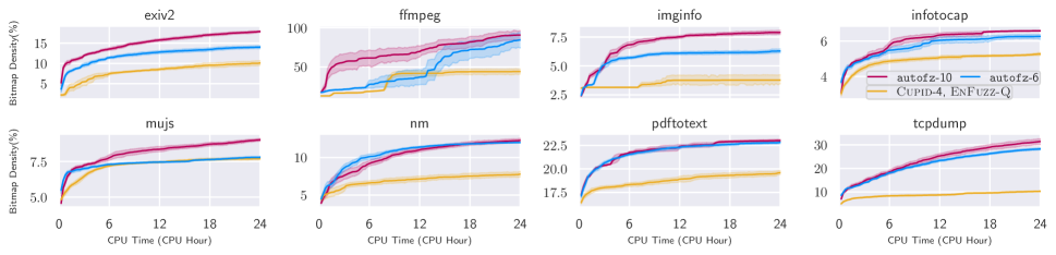
Figure 7: Comparison among autofz, EnFuzz, and Cupid on UniFuzz. Each line plot is depicted with an arithmetic mean and 80% confidence interval for 10 times fuzzing runs. The coverage ratio is the percentage of branches explored by each fuzzer. X-axis is elapsed CPU time. Below is the list of fuzzers used by different configurations: autofz-6 = [AFL, FairFuzz, QSYM, AFLFast, LAF-Intel, Radamsa ], Cupid-4 and EnFuzz-Q = [AFL, FairFuzz, QSYM, AFLFast ], autofz-10 = [All baseline fuzzers described in § 6 except libFuzzer ]

In the third preparation phase, QSYM exhibits reasonably good performance compared to the others ($diff_{peak},116$). However, most of the baseline fuzzers achieve similar coverage during the preparation phase (see the graph for prep round 3), and it cannot exceed the threshold ($\theta,300$) to exit early in the third preparation phase. Therefore, autofz decides to allocate the resources proportionally based on the trends of each individual fuzzer, unlike the first two rounds dedicating all resources to a sole fuzzer.

Slow but gradually improving fuzzers. Depending on the complexity of the baseline fuzzers, the time assigned for preparation phases might not be sufficient to build internal metrics. For example, QSYM requires a long initialization time for its concolic executor to build up internal states. Moreover, the concolic executor is designed to solve hard branches, so it might not be efficient to explore easy branches, which causes the other lightweight fuzzers to be selected until easy branches are resolved. As a result, fuzzers like QSYM can be treated as relatively underperforming, especially in the first few rounds or when the early exit occurs frequently, which causes it not to be selected in the focus phase and further prevents it from building up an internal state. However, thanks to the dynamic nature of autofz, it will allocate more time resources for preparation phases when other fuzzers become saturated (i.e., resolving all easy branches) and naturally take care of such slow but gradually improving fuzzers. As shown in Figure 13, QSYM has not been selected in most of the early rounds, but all resources are assigned to it in later rounds (i.e., 12 and 15).

6.5 Comparison with Collaborative Fuzzing

In this section, we compare autofz with collaborative fuzzing such as EnFuzz and Cupid for UniFuzz and FTS targets. We describe the result of UniFuzz to demonstrate that the prior knowledge utilized in collaborative fuzzing can be a major hindrance to efficient and automatic fuzzer selection. We also present the comparison for FTS targets in § A.2.

CPU hours..CPU hours.CPU hours.. We utilize the multi-core implementation of autofz because collaborative fuzzing concurrently deploys multiple fuzzers. To further achieve fairness in comparison, we fixed the total CPU time to 24 hours. The CPU time represents the total time resources consumed by all cores in each configuration. For example, autofz-6 and Cupid utilize six and four cores each; if we execute both configurations in physical 24 hours, each configuration spends 6*24 and 4*24 CPU hours, respectively, which is unfair to Cupid. Therefore, we make all evaluations run 24 CPU hours in total. If one configuration utilizes $N$ cores, each core can run $\frac{24}{N}$ hours.

Fuzzer selections for UniFuzz Since the evaluations and fuzzer selection of Cupid and EnFuzz target FTS, we cannot directly adopt the set of fuzzers depicted as the best in their works. Note that their best configurations include libFuzzer, and UniFuzz does not support it. Therefore, instead of libFuzzer, we selected LAF-Intel for autofz-6 and Cupid-4 in addition to five fuzzers utilized as the baseline in both works. For Cupid, we additionally retrieve its artifact and select the best four-fuzzer combination reported by the artifact. The detailed list of fuzzers and evaluation results is illustrated in Figure 7. We used the same set of fuzzers depicted as the best in their works in comparison for FTS targets (refer to  Figure 14) because FTS supports libFuzzer.

No prior knowledge, but a promising result..No prior knowledge, but a promising result.No prior knowledge, but a promising result.. The set of fuzzers selected by Cupid-4 is derived from the baseline fuzzers used by autofz-6, relying on offline analysis. However, autofz-6 outperforms Cupid-4 by 83.63% without any prior knowledge (see Table 4). Considering that autofz-6 and Cupid-4 achieves similar result for FTS targets (see Figure 14), we can infer that prior knowledge used in fuzzer selection is not diverse enough to represent real-world binaries. Note that the training set used by Cupid is generated as a result of running a subset of FTS targets; thus it can be biased toward FTS and cannot reduce the chance of overfitting when fuzzing UniFuzz targets. Our evaluation empirically demonstrates that, when relying on prior knowledge in fuzzer selection, results can be suboptimal and cannot guarantee the best outcome independent of the targets. Moreover, autofz makes evident that runtime trends are more reliable and cost-effective than well-established prior knowledge in fuzzer selection. Also, note that the selected set of fuzzers for Cupid-4 is the same as EnFuzz-Q, one of the configurations handpicked by the EnFuzz authors. This further indicates that expert-guided, target-specific combinations are unreliable and do not yield the best outcomes.

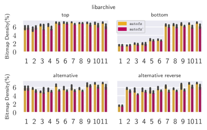
Figure 8: Evaluation of autofz and autofz^- on different numbers of baseline fuzzers. The target is libarchive. The X-axis indicates the number of fuzzers included to the baseline. The bar plots represent the average bitmap density across 10 executions. The accompanied error bars are generated with an 80% confidence interval. At $x=1$, autofz and autofz^- are identical. It is included as a baseline to be compared with different configurations.

6.6 Effects of the number of baseline fuzzers

As shown in Figure 14 and Figure 7, both autofz-11 and autofz-10 outperform autofz-6 in all benchmarks suites, except boringssl. This implies that adding more fuzzers will achieve better coverage in general due to the different natures induced by various fuzzers. However, the relationship between the number of fuzzers and their performance is not straightforward. This relationship can also be affected by how effective the resource scheduling algorithm of autofz is. Therefore, we introduce an autofz^-, a variant of autofz, which equally allocates resources to all baseline fuzzers in round-robin fashion. In this section, we evaluate autofz and autofz^- with various numbers of baseline fuzzers to provide a profound understanding of how this number can affect their performance in accordance with the underlying resource allocation algorithm. Also, we provide two thorough case studies.

Evaluation compositions..Evaluation compositions.Evaluation compositions.. In evaluating delta induced by having another baseline fuzzer, what fuzzer will be included to the baseline is important. For example, introducing a well-performing fuzzer gives a high chance of performance increase, but adding a bad fuzzer will not guarantee an improvement as much as the good one. Therefore, we test autofz and autofz^- with four different sequences in fuzzer addition: top, bottom, alternative, and alternative reverse. We explain the differences of these four different sequences using libarchive as an example. We evaluate each fuzzer’s performance based on Figure 3. The top sequence introduces fuzzers in descending order of performance: Redqueen, LAF-Intel, libFuzzer, QSYM, Angora, MOpt, LearnAFL, FairFuzz, AFL, AFLFast, and Radamsa. Conversely, the bottom brings in new fuzzers in ascending order (from the least coverage). For alternative, it selects one in the best and the next one in the worst, alternatively. For example, it selects Redqueen (1), Radamsa (11), LAF-Intel (2), AFLFast (10) $\cdots$. The alternative reverse, selects the one in the worst and the next one in the best one by one. Therefore, the order will be Radamsa (11), Redqueen (1), AFLFast (10), LAF-Intel (2) $\cdots$.

autofz versus autofz^-. The comparison between autofz and autofz^-, described in Figure 8, highlights the importance of resource allocation. It demonstrates that autofz can outperform autofz^- in most of the cases if both utilize the same fuzzer set. With the top and bottom cases, we see that the performance difference between autofz and autofz^- is not very large initially but increases as more fuzzers are introduced. The performance gap between autofz and autofz^- is much larger in the alternative and alternative reverse cases in almost all cases. Remember that autofz^- equally distributes resources to all baseline fuzzers, but autofz can redistribute resources based on the trends of individual fuzzers per workload. Therefore, fewer resources will be assigned to well-performing fuzzers as more fuzzers are introduced in autofz^-. This shows that autofz can prioritize well-performing fuzzers and relegate poorly performing fuzzers automatically on account of its clever resource allocation algorithm. We present further evaluations on nm and exiv2 in Figure 15.

(a) 5-fuzzers (Redqueen, Radamsa, LAF-Intel, AFLFast, libFuzzer)

(b) 6-fuzzers (5 fuzzers in 9(a) plus AFL)

Figure 9: Each pie chart presents the aggregated results across all rounds of the focus phases and overall fuzzing campaign (including preparation phases), respectively. The heat map describes the resource allocation determined by every round of the preparation phase. All figures are populated with data presented in Figure 8 with the alternative order setting. All data unit is %. (total 100%).

Case study: adding good fuzzer (5-fuzzers)..Case study: adding good fuzzer (5-fuzzers).Case study: adding good fuzzer (5-fuzzers).. In the following case studies, we further explain how autofz can exfiltrate well-performing fuzzers from various fuzzer sets. When it comes to 4-fuzzer and 5-fuzzer cases in the alternative order setting in Figure 8, we see huge coverage increases in autofz and autofz^- as a result of introducing one more good fuzzer, libFuzzer (ranked at 3). However, autofz experiences a much higher performance increase compared to autofz^-. We provide a reasonable explanation with 9(a) focusing on the resource allocation details of autofz. First, autofz rarely allocates resources to poorly performing fuzzers (i.e., Radamsa and AFLFast). Note that autofz consumed only 6% and 2% of resources for the bad fuzzers during the entire focus phases. Even after taking the preparation phases into account, autofz spent only 22% resources total for the two bad fuzzers. However, autofz^- equally distributed the resources, 20% for each fuzzer, regardless of their performance. Therefore, autofz^- spent 18% more resources on the poorly performing fuzzers. Second, autofz allocated more resources toward three well-performing fuzzers (i.e., Redqueen, LAF-Intel, libFuzzer), which boosts the performance. The first pie chart shows that autofz respectively allocated 35%, 30%, and 27% of resources to them during the entire focus phases. Note that more resources were allotted to better-performing fuzzers even though autofz does not have any prior knowledge about which fuzzers are in what ranks. However, autofz^- equally assigns 20% of resources to each of the three fuzzers. For total resources spent for those three fuzzers, autofz and autofz^- consumed 78% and 60%, respectively.

Case study: adding bad fuzzer (6-fuzzers).Case study: adding bad fuzzer (6-fuzzers)Case study: adding bad fuzzer (6-fuzzers). Contrary to the previous case study, we explain how autofz and autofz^- react when a poorly performing fuzzer is introduced to their baseline. As described in Figure 9, we added one more fuzzer AFL (ranked at 9) and captured how the coverage changes. After the addition, both autofz and autofz^- had a performance drop. The resource allocation detail is shown in 9(b). autofz allocates only 2% of resources to AFL during the entire focus phase, which demonstrates that it can exfiltrate poorly performing fuzzers properly. However, when it comes to overall resources spent for AFL, it increases to 8%, which is the major reason for the slowdown. In this example, autofz spent 6% of resources to capture possible trend changes during the preparation phases. Note that this cost is unavoidable. Therefore, as more fuzzers are introduced, the resources spent for the preparation phases can become a burden for autofz. However, the captured runtime trend more than compensates for the slowdown incurred by the preparation phases. As a consequence, autofz still outperforms autofz^- after introducing AFL, which demonstrates that the resource allocation algorithm of autofz can highlight good fuzzers.

6.7 Bug Discovery Evaluation

To compare the number of bugs found by autofz and individual fuzzers, we run ASan-instrumented FTS and UniFuzz targets and collect generated crashes. We triage the crashes and measure deduplicated bugs by taking the top three stack frames and using them as unique identifiers for the bugs. autofz found the most bugs on average compared to individual fuzzers, Cupid, and EnFuzz. Moreover, when we aggregate the results of all 10 fuzzing repetitions, autofz still uncovered the most bugs, some of which are not found by any individual fuzzer. The detailed results are in § A.6.

6.8 Evaluation of autofz decision

In this section, we evaluate how accurate the decisions of autofz are in terms of resource allocation . Resource allocation is the essence of autofz because it reflects the trends of baseline fuzzers and makes a subset of baseline fuzzers to be online predicted to be efficient for the current workload. If prediction about runtime trends is inaccurate and does not continue, less coverage will be explored. Therefore, we can estimate the continuity of measured trends as the end result achieved as a result of deploying specific resource allocation per round. However, it is not practical to compare autofz with all possible resource allocation decisions because it is infinite. To this end, we carefully design the following evaluation.

1. For each round, record when the preparation phase ended ($time_{\_}{prep\_end}$) and total time budget assigned for the focus phase ($time_{\_}{focus\_total}$). Note that the value of these two variables can be different in every round based on when the early exit occurs.

2. Collect all output corpus created earlier than $time_{\_}{prep\_end}$. We call it snapshot. The snapshot restores the full status of the fuzzing campaign to the state right before the focus phase.

3. For the number of baseline fuzzers, repeat the below procedures.

   1. Select one fuzzer and update resource allocation so that all resources are assigned to that fuzzer.

   2. Run the fuzzer for $time_{\_}{focus\_total}$ and measure the coverage. Note that each individual fuzzer run represents synthetic decisions made for comparison.

   3. Restore the current state to right before the focus phase using the snapshot.

4. Lastly, run fuzzers selected by the resource allocation of autofz for $time_{\_}{focus\_total}$ and measure the coverage.

The evaluation results on libarchive and exiv2 are presented in 10(a) and 10(b), respectively. As shown in 10(a), the decision made by autofz allows it to take first place eight times over 14 rounds and rank 2.64 on average. The exiv2 target, presented in 10(b), ranks 3.5 on average and took first place four times over 15 rounds. This result demonstrates that the decision of autofz is effective compared with others and proves that the captured trends maintain until the next measurement.

Saturation and effectiveness of autofz The result shows that the allocation decisions of autofz become less efficient as the number of new coverage reported by the baseline fuzzer saturates. Although autofz ranks higher on average in fuzzing libarchive compared to exiv2, note that AFL bitmap count saturates faster in exiv2 than in libarchive. In detail, after round 4 in exiv2, all different decisions including autofz do not exhibit meaningful bitmap coverage increases. Therefore, no matter which fuzzers are activated as a result of different resource allocations, it is difficult to make progress after round 4. For example, autofz ranked 11 in round 15, but the bitmap density difference between LAF-Intel (the best) and autofz (the worst) is only 0.07%.

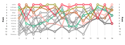
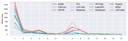
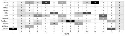
(a) Evaluation of autofz decision on libarchive

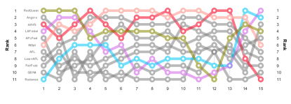
(b) Evaluation of autofz decision on exiv2

Figure 10: Comparison between resource allocation decision of autofz (Algorithm 2) and decisions allocating entire resources to each baseline fuzzers. The bump chart compares the ranks of all decisions in terms of AFL bitmap coverage. We highlight decisions that have ranked top at least once. The line plots illustrate bitmap counts of different decisions at each round. The heatmap presents autofz’s detailed resource allocation decisions. Note that the allocation reflects runtime trends of different fuzzer at each round.

Noise introduced by inherent randomness..Noise introduced by inherent randomness.Noise introduced by inherent randomness.. Although we carefully designed our evaluation so that all different decisions have identical starting lines using snapshot every round, it is impossible to completely prevent introducing noise due to the inherent randomness in fuzzing campaigns. For example, in 10(a), autofz allocates all resources to libFuzzer at the first round, making autofz’s decision identical to the libFuzzer case. However, the result of following autofz’s decision (ranked 1) slightly outperforms the libFuzzer decision (ranked 2), as shown in 10(a). We believe that the inherent randomness, such as in input mutations, causes this difference, which we call noise.

Seed synchronization might change the trends..Seed synchronization might change the trends.Seed synchronization might change the trends.. We can explain why the captured trends sometimes will not be sustained in two aspects. First, the preparation phase was not long enough to capture the trends properly. Second, autofz captured the trends accurately, but the seed synchronization after the preparation allows the other individual fuzzers to report strong trends. For example, we can observe that Redqueen does not perform well compared to Angora when each fuzzer runs individually, highlighted in § 6.4. The first round of the preparation on exiv2 reports that Angora exhibits the strongest trend, which follows the observations. Therefore, autofz allocates all resources to Angora (see the heatmap presented in 10(b)). However, our evaluation revealed that Redqueen performed the best during the first round of the focus phase (see the second graph of 10(b)). Note that this result does not follow our initial observation. We believe that this happens because the first round of the preparation phase explored paths that used to be challenging for Redqueen to resolve. Therefore, after the seed synchronization, Redqueen does not need to spend its resources to reach those paths anymore and exhibit the strongest trends during the focus phase. However, note that Angora still performs well in the first focus phase even though it cannot be ranked on top. This demonstrates that runtime trends captured in the preparation phase are strong enough to allow autofz to achieve good performance.

7 Discussion

We discuss the limitations and future works of autofz.

Metric diversity. autofz utilizes AFL bitmap to compare runtime trends, which favors the fuzzers that seek to maximize path coverage. While the coverage is the most popular and explicit indicator of progress in fuzzing, relying on a single metric can potentially lead to unfair comparison with various fuzzers utilizing metrics other than the coverage [45, 16, 46, 47, 38]. Therefore, supporting multiple metrics besides path coverage can achieve fairness and better efficiency in terms of resource allocation. For example, different metrics can be used to break the tie, especially when one metric is saturated.

Bad fuzzer elimination. A particular fuzzer might not perform well throughout the fuzzing for specific targets (e.g., Radamsa on exiv2 shown in Figure 3). autofz automatically prevents poorly performing fuzzers from being online during the focus phase through resource allocation. However, the same amount of resources are allocated to all baseline fuzzers during the preparation phase to measure runtime trends. If poorly performing fuzzers can be eliminated from the baseline timely, autofz can achieve better resource utilization.

8 Conclusion

This paper presented autofz, a meta-fuzzer providing fine-grained and non-intrusive fuzzer orchestration. Our evaluation result illustrates that automated fuzzer composition without any prior knowledge is effective. By observing the trends of fuzzers at runtime and distributing the computing resources properly, autofz has not only beat the individual fuzzers but also the state-of-the-art collaborative fuzzing approaches. We expect that autofz can bridge the gap between developing new fuzzers and their effective deployment.

Appendix A Appendix

Algorithm 3 Two Phase Algorithm

1:Input

2:  $\mathbb{F}\leftarrow\{{f_{\_}{1},f_{\_}{2},...,f_{\_}{n}\}}$, $f_{\_}{n}$ is instance of $n_{\_}{th}$ baseline fuzzer

3:  $\mathbb{B}\leftarrow\{{b_{\_}{1},b_{\_}{2},...,b_{\_}{n}\}}$, $b_{\_}{n}$ is bitmap of $f_{\_}{n}$

4:  $T_{\_}{prep,focus}\leftarrow$ Time budget for preparation/focus phase

5:  $\theta_{\_}{init,cur}\leftarrow$ Initial and current threshold

6:  $C\leftarrow$ How many CPU cores are assigned

7:function autofzmain($\mathbb{F}$, $T_{\_}{prep}$, $T_{\_}{focus}$, $\theta_{\_}{cur}=\theta_{\_}{init}$, $C$)

8:  while NOT timeout do

9:    seed_sync($\mathbb{F}$)

10:    $Exit_{\_}{early}$, $T_{\_}{remain}$ $\leftarrow$ prep_phase($\mathbb{F}$, $\mathbb{B}$, $T_{\_}{prep}$, $\theta_{\_}{cur}$, $C$)

11:    $\mathbb{RA}\leftarrow\textsc{resource\_allocator}(\mathbb{F},\mathbb{B},Exit_{\_}{early})$

12:    $\theta_{\_}{cur}\leftarrow$ $(Exit_{\_}{early})$ $?$ $\theta_{\_}{cur}+\theta_{\_}{init}$ $:$ $\theta_{\_}{cur}*0.5$ $\triangleright$ AIMD

13:    seed_sync($\mathbb{F}$)

14:    focus_phase($\mathbb{F}$, $\mathbb{RA}$, $T_{\_}{focus}+T_{\_}{remain}$, $C$)   

Algorithm 4 Focus Phase

1:function focus_phase($\mathbb{F}$, $\mathbb{RA}$, $T_{\_}{focus}$, $C$)

2:  if $C==1$ then

3:    $T_{\_}{focus\_total}\leftarrow T_{\_}{focus}\times\textsc{num\_of\_fuzzers}(\mathbb{F})$

4:     $\mathbb{F}$ $\leftarrow$ sort_fuzzers($\mathbb{F}$, key = $\mathbb{RA}$, order = descending)

5:    for each $f$ $\in$ $\mathbb{F}$ do

6:      $T_{\_}{run}\leftarrow T_{\_}{focus\_total}\times\mathbb{RA}[f]$

7:      if $T_{\_}{run}>0$ then

8:         $\textsc{run\_fuzzer}(f,T_{\_}{run})$

9:         $\textsc{seed\_sync}(\mathbb{F})$           

10:  else$\triangleright$ multi-core implementation

11:    $c\leftarrow C\times\mathbb{RA}[f]$

12:    run_fuzzers_parallel_seed_sync($\mathbb{F}$, $T_{\_}{focus}$, $c$)

13:    $\textsc{seed\_sync}(\mathbb{F})$   

A.1 Queue Size Statistics And Observation

Queue size measurement..Queue size measurement.Queue size measurement.. We collect files in queue output directories to measure changes in queue size over 24 hours. Whenever an interesting seed is found, each fuzzer stores the seed as a file in the queue directory. Each fuzzer has a different guideline to determine which seed is interesting, for example, based on whether a seed explores new coverage. autofz has no clear definition of interesting seeds, so it collects all interesting seeds from the queue directories of all baseline fuzzers and deduplicates the same seeds by comparing their hash. Figure 18 presents the queue size change over 24 hours for autofz and individual fuzzers on UniFuzz and FTS.

Observation.ObservationObservation. We found that Angora significantly outperforms other fuzzers, including autofz, in terms of queue size on freetype2, pdftotext, mujs, and tcpdump. However, Angora embarrassingly underperforms in terms of line and edge coverage on those targets except tcpdump. We analyzed the logs of Angora and found that, especially when the coverage saturates, it generated lots of new seeds contributing a tiny fraction of the context-sensitive coverage bitmap. For example, in mujs, Angora generated around $80,000$ interesting seeds and achieved 99.98% bitmap coverage. However, it requires around $90,000$ interesting seeds to cover the remaining 0.02% bitmap coverage.

Possible interpretation.Possible interpretationPossible interpretation. We speculate that abundant seeds hinder Angora from mutating the seeds that could be meaningful in terms of other metrics. For example, such high bitmap density can lead to a higher rate of hash collision and prevent interesting seeds in terms of different metrics from being generated. As a result, Angora underperforms on freetype2, pdftotext, mujs in terms of AFL bitmap density, edge coverage, and bug-finding because the context-sensitive coverage bitmap of Angora saturates early. On the other hand, for tcpdump, Angora outperforms others not only in queue size but also in bug finding. This result implies that considering multiple metrics in autofz could be beneficial in terms of finding bugs.

Figure 11: The graph shows a critical difference (CD) among the various configuration of autofz. Each pair represents the three configurations; for example, (300, 600, 200) means $T_{\_}{prep}=300$, $T_{\_}{focus}=600$, $\theta_{\_}{init}=200$. The CD diagram demonstrates that there is no statistical difference among the tested configurations (all configurations are grouped in one line).

Figure 12: Critical Difference for the targets in FTS

Round	Winner	$diff_{peak}$	$\theta$	$T_{prep}$	$T_{focus}$
$1^{*}$	Angora	857	100	30	570
$2^{*}$	Redqueen	234	200	150	450
3	None	116	300	300	300
4	None	48	150	300	300
$5^{*}$	Redqueen	92	75	300	300
6	None	30	175	300	300
7	None	22	87.5	300	300
8	None	26	43.75	300	300
$9^{*}$	LAF-Intel	71	21.88	90	510
10	None	31	121.88	300	300
11	None	21	60.94	300	300
12	None	24	30.47	300	300
$13^{*}$	LAF-Intel	27	15.23	300	300
14	None	12	115.23	300	300
15	None	40	57.62	300	300

* asterisk mark after the round numbers means that $Exit_{\_}{early}$ is true.

Figure 13: Full result of Figure 6. $\theta$ is rounded to two decimal places

A.2 Comparison of autofz and collaborative fuzzing on FTS targets

Figure 14: Comparison among autofz, EnFuzz, and Cupid. Each line plot is depicted with an arithmetic mean and 80% confidence interval for 10 times fuzzing runs. The coverage ratio is a percentage of branches explored by each fuzzer. X-axis is elapsed CPU time. Below is the list of fuzzers used by different configurations: autofz-6 = [AFL, FairFuzz, QSYM, AFLFast, libFuzzer, Radamsa ], Cupid-4 = [AFL, FairFuzz, QSYM, libFuzzer ], EnFuzz-4 = [AFL, FairFuzz, Radamsa, libFuzzer ] which is reported to be the best in [10], autofz-11 = [All baseline fuzzers described in § 6]

benchmark	autofz-11	autofz-6	Cupid-4	EnFuzz-4
boringssl	1.85	1.85	1.88	1.89
freetype2	9.88	9.26	8.85	8.43
guetzli	3.96	3.90	3.84	3.90
json	1.09	1.08	1.09	1.08
lcms	2.36	2.17	2.15	1.92
libarchive	6.74	5.30	6.23	4.83
libjpeg	2.15	2.13	2.14	1.99
libpng	1.18	1.14	1.14	1.08
re2	3.42	3.40	3.41	3.40
vorbis	1.56	1.56	1.55	1.54
woff2	1.62	1.58	1.54	1.54
wpantund	6.53	6.17	5.79	6.12
SUM	42.35	39.55	39.61	37.72
IMPROVE	+12.27%	+4.85%	+5%	-

Table 2: Bitmap density of autofz, Cupid, and EnFuzz on FTS corresponding to Figure 14. The bitmap density is presented as a percentage.

	autofz-11		autofz-6
benchmark	Cupid-4	EnFuzz-4	Cupid-4	EnFuzz-4
boringssl	< 0.01	0.03	< 0.01	0.02
freetype2	< 0.01	< 0.01	< 0.01	< 0.01
guetzli	< 0.01	< 0.01	< 0.01	0.76
json	< 0.01	< 0.01	0.02	0.02
lcms	< 0.01	< 0.01	0.76	< 0.01
libarchive	0.05	< 0.01	0.06	< 0.01
libjpeg	0.97	< 0.01	0.45	< 0.01
libpng	< 0.01	< 0.01	0.97	< 0.01
re2	0.20	0.02	0.32	1.00
vorbis	0.27	0.15	0.40	< 0.01
woff2	0.03	0.02	< 0.01	< 0.01
wpantund	< 0.01	0.01	< 0.01	0.35

Table 3: Mann-Whitney U Test evaluated on FTS based on the bitmap result presented in Table 2. The left two columns compare autofz-11 with Cupid-4 and EnFuzz-4. The right two columns compares autofz-6 and the others. The results showing a statistical difference are in bold.

A.3 Comparison of autofz and collaborative fuzzing on UniFuzz targets

benchmark	autofz-10	autofz-6	Cupid-4 &
			EnFuzz-Q
exiv2	19.67	14.56	10.18
ffmpeg	99.52	99.27	44.24
imginfo	8.32	6.45	3.77
infotocap	6.64	6.32	5.27
mujs	9.56	7.91	7.71
nm	13.28	12.27	7.81
pdftotext	24.20	23.20	19.67
tcpdump	37.74	30.13	10.32
SUM	218.91	200.11	108.97
IMPROVE	+100.9%	+83.63%	-

Table 4: Bitmap density of autofz, Cupid, and EnFuzz-Q (same as Cupid-4, omitted) on UniFuzz corresponding to Figure 7. The bitmap density is presented as a percentage.

	autofz-10	autofz-6
benchmark	Cupid-4	Cupid-4
exiv2	< 0.01	< 0.01
ffmpeg	< 0.01	< 0.01
imginfo	< 0.01	< 0.01
infotocap	< 0.01	< 0.01
mujs	< 0.01	0.05
nm	< 0.01	< 0.01
pdftotext	0.04	< 0.01
tcpdump	< 0.01	< 0.01

Table 5: Mann-Whitney U Test evaluated on UniFuzz based on the bitmap result presented in Table 4. The left two columns compare autofz-10 with Cupid-4 and EnFuzz-Q (same as Cupid-4, omitted). The right two columns compare autofz-6 and the others. The results showing statistical difference are in bold.

A.4 Detail Coverage and Mann-Whitney U Test among autofz and individual fuzzers

benchmark	autofz	AFL	AFLFast	Angora	FairFuzz	LAF-Intel	LearnAFL	MOpt	QSYM	Radamsa	RQ	Lib
exiv2	18.84	9.35	4.90	12.84	11.41	13.69	9.80	11.53	8.49	1.89	14.90	-
ffmpeg	100.00	44.08	46.11	25.60	49.74	79.83	100.00	60.37	20.32	54.80	88.85	-
imginfo	7.82	2.65	2.47	5.55	3.05	6.62	6.01	5.27	3.47	3.89	7.81	-
infotocap	6.19	4.75	5.03	3.92	5.40	5.70	5.82	5.54	4.81	3.95	6.08	-
mujs	8.88	7.20	7.25	4.55	8.17	7.65	7.89	7.77	7.24	7.11	8.22	-
nm	12.19	6.14	5.80	6.58	6.92	10.59	9.14	11.01	7.85	4.45	10.73	-
pdftotext	24.02	19.37	19.46	16.99	19.11	23.09	23.95	19.98	18.40	20.47	26.77	-
tcpdump	36.30	9.34	9.31	29.25	9.85	30.09	29.57	26.38	8.63	9.98	31.92	-
tiffsplit	7.56	5.97	6.03	4.98	6.38	6.57	6.75	6.80	6.33	3.89	6.45	-
boringssl	1.89	1.80	1.79	1.79	1.81	1.83	1.80	1.83	1.79	1.78	1.84	1.87
freetype2	9.87	6.31	6.55	5.61	7.09	7.36	7.37	7.47	7.81	5.84	9.73	8.38
libarchive	6.91	2.36	2.13	3.31	2.87	4.78	3.11	3.07	4.31	1.67	5.72	5.21

Table 6: Bitmap density of autofz and individual fuzzers corresponding to Figure 3. Each number represents bitmap density in percentage. The best result of each benchmark suite is in bold in the table. RQ and LIB indicate Redqueen and libFuzzer, respectively.

benchmark	AFL	AFLFast	Angora	FairFuzz	LAF-Intel	LearnAFL	MOpt	QSYM	Radamsa	RedQueen	LibFuzzer
exiv2	< 0.01	< 0.01	< 0.01	< 0.01	< 0.01	< 0.01	< 0.01	< 0.01	< 0.01	< 0.01	-
ffmpeg	< 0.01	< 0.01	< 0.01	0.01	< 0.01	0.29	< 0.01	< 0.01	< 0.01	< 0.01	-
imginfo	< 0.01	< 0.01	< 0.01	< 0.01	< 0.01	< 0.01	< 0.01	< 0.01	< 0.01	0.24	-
infotocap	< 0.01	< 0.01	< 0.01	< 0.01	0.03	0.03	< 0.01	< 0.01	< 0.01	0.09	-
mujs	< 0.01	< 0.01	< 0.01	< 0.01	< 0.01	< 0.01	< 0.01	< 0.01	< 0.01	< 0.01	-
nm	< 0.01	< 0.01	< 0.01	< 0.01	< 0.01	< 0.01	< 0.01	< 0.01	< 0.01	0.01	-
pdftotext	< 0.01	< 0.01	< 0.01	< 0.01	< 0.01	0.60	< 0.01	< 0.01	< 0.01	< 0.01	-
tcpdump	< 0.01	< 0.01	< 0.01	< 0.01	< 0.01	< 0.01	< 0.01	< 0.01	< 0.01	< 0.01	-
tiffsplit	< 0.01	< 0.01	< 0.01	< 0.01	< 0.01	< 0.01	< 0.01	< 0.01	< 0.01	< 0.01	-
boringssl	< 0.01	< 0.01	< 0.01	< 0.01	< 0.01	< 0.01	< 0.01	< 0.01	< 0.01	< 0.01	0.60
freetype2	< 0.01	< 0.01	< 0.01	< 0.01	< 0.01	< 0.01	< 0.01	< 0.01	< 0.01	0.34	< 0.01
libarchive	< 0.01	< 0.01	< 0.01	< 0.01	< 0.01	< 0.01	< 0.01	< 0.01	< 0.01	< 0.01	< 0.01

Table 7: Mann-Whitney U Test results evaluated based on the result presented in Table 6. A value less than 0.05 indicates the result is statistically different between autofz and the selected fuzzer. The results showing statistical difference are in bold.

A.5 Effects of the number of baseline fuzzers for exiv2 and nm

  

Figure 15: Evaluation of autofz and autofz^- on different numbers of baseline fuzzers (1-10) for exiv2 and nm.

A.6 Unique Bug Count among autofz, individual fuzzers, and collaborative fuzzing

Average number of unique bugs.Average number of unique bugsAverage number of unique bugs. The unique bugs represent all deduplicated bugs found by a specific fuzzer. We compare the average number of unique bugs of autofz and others in 10 repetitions (Table 8, Table 10, and Table 12). The result shows that autofz can outperform individual fuzzers and collaborative fuzzing such as EnFuzz and Cupid for bug finding.

Aggregated unique bug counts..Aggregated unique bug counts.Aggregated unique bug counts.. In addition to the average number of unique bugs, we also aggregate all unique bugs found by each fuzzer in 10 repetitions. We present the numbers in three different categories per individual fuzzer: the number of unique bugs, the number of exclusive bugs, and the number of unobserved bugs (Table 9, Table 11, and Table 11). The exclusive bugs means the bugs that cannot be found by other fuzzers, but only by this fuzzer. The unobserved bugs are the bugs that cannot be found by this fuzzer, but are reported by the others.

Bug report.Bug reportBug report. We could not find a new bug because UniFuzz and FTS consist of old versions of programs, and most of the bugs have been already reported and fixed. We reproduced the found bug on the latest version of the targets and confirmed that all of the bugs we found are not present in the latest version.

benchmark	autofz	AFL	AFLFast	Angora	FairFuzz	LAF-Intel	LearnAFL	MOpt	QSYM	Radamsa	RQ	Lib
exiv2	13.10	2.50	1.50	7.10	3.10	5.60	2.70	4.30	0.00	0.10	6.40	-
ffmpeg	0.20	0.00	0.00	0.00	0.00	0.80	0.20	0.00	0.00	0.00	0.80	-
imginfo	0.80	0.00	0.00	0.00	0.20	1.00	0.60	0.30	0.00	0.00	1.00	-
infotocap	5.50	2.50	2.70	0.00	3.60	2.30	3.90	3.60	0.00	0.30	3.20	-
mujs	3.00	0.00	0.50	0.00	0.30	2.00	0.60	0.80	0.00	4.20	0.70	-
nm	0.50	0.00	0.00	0.70	0.00	0.10	0.00	0.10	0.00	0.00	0.20	-
pdftotext	3.70	1.50	1.60	1.20	1.40	6.80	6.50	1.90	0.00	2.30	9.10	-
tcpdump	1.90	0.00	0.00	2.30	0.00	1.50	1.00	1.50	0.00	0.00	0.70	-
tiffsplit	6.20	2.90	2.90	3.50	3.50	3.80	4.70	3.90	0.00	1.40	3.50	-
boringssl	0.40	0.00	0.00	0.00	0.00	0.00	0.00	0.00	0.00	0.00	0.00	0.20
freetype2	0.00	0.00	0.00	0.00	0.00	0.00	0.00	0.00	0.00	0.00	0.00	0.00
libarchive	0.40	0.00	0.00	0.00	0.00	0.30	0.00	0.00	0.00	0.00	0.70	0.40
SUM	35.70	9.40	9.20	14.80	12.10	24.20	20.20	16.40	0.00	8.30	26.30	0.60

Table 8: The average number of unique bugs found by autofz and individual fuzzers in 10 repetitions. The RQ and LIB indicate Redqueen and libFuzzer, respectively.

benchmark	autofz	AFL	AFLFast	Angora	FairFuzz	LAF-Intel	LearnAFL	MOpt	QSYM	Radamsa	RQ	Lib
exiv2	31/4/11	8/0/34	8/0/34	20/3/22	9/0/33	23/3/19	13/1/29	16/0/26	0/0/42	1/0/41	17/1/25	-
ffmpeg	2/0/2	0/0/4	0/0/4	0/0/4	0/0/4	2/0/2	2/1/2	0/0/4	0/0/4	0/0/4	3/1/1	-
imginfo	1/0/0	0/0/1	0/0/1	0/0/1	1/0/0	1/0/0	1/0/0	1/0/0	0/0/1	0/0/1	1/0/0	-
infotocap	9/0/1	3/0/7	3/0/7	0/0/10	7/1/3	5/0/5	7/0/3	5/0/5	0/0/10	1/0/9	6/0/4	-
mujs	6/0/4	0/0/10	1/0/9	0/0/10	1/0/9	3/0/7	1/0/9	2/0/8	0/0/10	9/4/1	1/0/9	-
nm	2/1/8	0/0/10	0/0/10	6/4/4	0/0/10	1/0/9	0/0/10	1/1/9	0/0/10	0/0/10	2/2/8	-
pdftotext	11/1/28	2/0/37	3/0/36	2/0/37	2/0/37	16/2/23	19/10/20	4/0/35	0/0/39	4/0/35	23/11/16	-
tcpdump	6/0/9	0/0/15	0/0/15	11/5/4	0/0/15	7/2/8	3/0/12	3/0/12	0/0/15	0/0/15	1/0/14	-
tiffsplit	8/0/3	5/0/6	6/1/5	6/0/5	6/0/5	6/1/5	8/1/3	5/0/6	0/0/11	3/0/8	8/0/3	-
boringssl	1/0/0	0/0/1	0/0/1	0/0/1	0/0/1	0/0/1	0/0/1	0/0/1	0/0/1	0/0/1	0/0/1	1/0/0
freetype2	0/0/0	0/0/0	0/0/0	0/0/0	0/0/0	0/0/0	0/0/0	0/0/0	0/0/0	0/0/0	0/0/0	0/0/0
libarchive	1/0/2	0/0/3	0/0/3	0/0/3	0/0/3	1/0/2	0/0/3	0/0/3	0/0/3	0/0/3	1/0/2	2/2/1
SUM	78/6/68	18/0/128	21/1/125	45/12/101	26/1/120	65/8/81	54/13/92	37/1/109	0/0/146	18/4/128	63/15/83	3/2/1

Table 9: Unique bug count of autofz and individual fuzzers aggregated over 10 fuzzing repetitions, corresponding to Figure 3. Each number in A/B/C indicates the following. A: the number of unique bugs. B: the number of exclusive bugs. C: the number of unobserved bugs.

benchmark	autofz-10	autofz-6	Cupid-4 &
			EnFuzz-Q
exiv2	16.70	5.80	2.70
ffmpeg	0.00	0.00	0.00
imginfo	0.70	0.10	0.00
infotocap	5.90	4.70	2.40
mujs	3.50	3.60	0.20
nm	1.20	0.00	0.00
pdftotext	4	3.80	1.10
tcpdump	1.00	0.50	0.00
SUM	33	18.5	6.4
IMPROVE	+415%	+189%	-

Table 10: Unique Bug Count of autofz, Cupid, and EnFuzz-Q (same as Cupid-4, omitted) on UniFuzz corresponding to Figure 7. Each number represents the average bug count across 10 fuzzing repetitions.

benchmark	autofz-10	autofz-6	Cupid-4 &
			EnFuzz-Q
exiv2	33/16/4	20/4/17	6/0/31
ffmpeg	0/0/0	0/0/0	0/0/0
imginfo	1/0/0	1/0/0	0/0/1
infotocap	7/1/2	8/2/1	5/0/4
mujs	6/1/2	7/2/1	1/0/7
nm	8/8/0	0/0/8	0/0/8
pdftotext	9/0/0	9/0/0	2/0/7
tcpdump	5/4/0	1/0/4	0/0/5
SUM	69/30/8	46/8/31	14/0/63
IMPROVE	+392%	+228%	-

Table 11: Aggregated unique bug count of autofz, Cupid, and EnFuzz-Q (same as Cupid-4, omitted) across 10 fuzzing repetitions on UniFuzz corresponding to Figure 7. Please refer to Table 9 for the meaning of cells.

benchmark	autofz-11	autofz-6	Cupid-4	EnFuzz-4
boringssl	0.00	0.00	0.20	0.40
freetype2	0.00	0.00	0.00	0.00
guetzli	1.10	1.10	0.60	1.10
json	1.00	1.00	1.00	1.00
lcms	0.00	0.00	0.00	0.00
libarchive	0.40	0.00	0.00	0.00
libjpeg	0.00	0.00	0.00	0.00
libpng	0.00	0.10	0.00	0.00
re2	0.30	0.00	0.10	0.30
woff2	0.50	0.30	0.20	0.40
vorbis	0.00	0.00	0.00	0.10
wpantund	0.00	0.00	0.00	0.00
SUM	3.3	2.5	2.1	3.3

Table 12: Unique Bug Count of autofz, Cupid, and EnFuzz on FTS corresponding to Figure 14. Each number represents the average bug count across 10 fuzzing repetitions.

benchmark	autofz-11	autofz-6	Cupid-4	EnFuzz-4
boringssl	0/0/2	0/0/2	1/0/1	2/1/0
freetype2	0/0/0	0/0/0	0/0/0	0/0/0
guetzli	2/0/0	2/0/0	1/0/1	2/0/0
json	1/0/0	1/0/0	1/0/0	1/0/0
lcms	0/0/0	0/0/0	0/0/0	0/0/0
libarchive	3/3/0	0/0/3	0/0/3	0/0/3
libjpeg	0/0/0	0/0/0	0/0/0	0/0/0
libpng	0/0/1	1/1/0	0/0/1	0/0/1
re2	1/0/0	0/0/1	1/0/0	1/0/0
woff2	1/0/0	1/0/0	1/0/0	1/0/0
vorbis	0/0/1	0/0/1	0/0/1	1/1/0
wpantund	0/0/0	0/0/0	0/0/0	0/0/0
SUM	8/3/4	5/1/7	5/0/7	8/2/4

Table 13: Aggregated unique bug count of autofz, Cupid, and EnFuzz across 10 fuzzing repetitions on FTS corresponding to Figure 14. Please refer to Table 9 for the meaning of cells.

A.7 Different metric other than AFL bitmap

To facilitate comparisons between autofz and existing results in the literature, we represent the results in three different metrics: edge coverage (Figure 16), line coverage (Figure 17), and queue size (Figure 18). We adopt the same configuration of autofz used in Figure 3. Each line plot is depicted with an arithmetic mean and 80% confidence interval for 10 times fuzzing executions.

Figure 16: Evaluation of autofz on UniFuzz and FTS in terms of edge coverage.

Figure 17: Evaluation of autofz on UniFuzz and FTS in terms of line coverage.

Figure 18: Evaluation of autofz on UniFuzz and FTS in terms of queue size.

References

- [1] “Circumventing fuzzing roadblocks with compiler transformations,” 2016, https://lafintel.wordpress.com/.
- [2] A. Arcuri, M. Z. Iqbal, and L. Briand, “Random testing: Theoretical results and practical implications,” IEEE Transactions on Software Engineering, 2012.
- [3] C. Aschermann, S. Schumilo, T. Blazytko, R. Gawlik, and T. Holz, “REDQUEEN: fuzzing with input-to-state correspondence,” in NDSS, 2019.
- [4] M. Boehme, C. Cadar, and A. ROYCHOUDHURY, “Fuzzing: Challenges and reflections,” IEEE Software, vol. 38, 2021.
- [5] M. Böhme, V. J. M. Manès, and S. K. Cha, “Boosting fuzzer efficiency: an information theoretic perspective,” in ESEC/FSE, 2020.
- [6] M. Böhme, V.-T. Pham, and A. Roychoudhury, “Coverage-based Greybox Fuzzing as Markov Chain,” in CCS, 2016.
- [7] M. Böhme, V. Pham, and A. Roychoudhury, “Coverage-based greybox fuzzing as markov chain,” IEEE Trans. Software Eng., vol. 45, 2019.
- [8] C. Cadar, D. Dunbar, and D. Engler, “KLEE: Unassisted and Automatic Generation of High-coverage Tests for Complex Systems Programs,” in OSDI, 2008.
- [9] P. Chen and H. Chen, “Angora: Efficient fuzzing by principled search,” in S&P Oakland, 2018.
- [10] Y. Chen, Y. Jiang, F. Ma, J. Liang, M. Wang, C. Zhou, X. Jiao, and Z. Su, “Enfuzz: Ensemble fuzzing with seed synchronization among diverse fuzzers,” in Security, 2019.
- [11] D.-M. Chiu and R. Jain, “Analysis of the increase and decrease algorithms for congestion avoidance in computer networks,” Computer Networks and ISDN systems, vol. 17, 1989.
- [12] DARPA, “DARPA Cyber Grand Challenge Final Event Archive,” 2016, https://www.lungetech.com/cgc-corpus/.
- [13] J. Demšar, “Statistical comparisons of classifiers over multiple data sets,” The Journal of Machine Learning Research, vol. 7, 2006.
- [14] Z. Ding and C. L. Goues, “An empirical study of oss-fuzz bugs,” in IEEE/ACM 18th International Conference on Mining Software Repositories (MSR), 2021.
- [15] B. Dolan-Gavitt, P. Hulin, E. Kirda, T. Leek, A. Mambretti, W. K. Robertson, F. Ulrich, and R. Whelan, “LAVA: large-scale automated vulnerability addition,” in S&P Oakland, 2016.
- [16] A. Fioraldi, D. C. D’Elia, and D. Balzarotti, “The use of likely invariants as feedback for fuzzers,” in Security, 2021.
- [17] A. Fioraldi, D. Maier, H. Eißfeldt, and M. Heuse, “AFL++ : Combining incremental steps of fuzzing research,” in USENIX Workshop on Offensive Technologies (WOOT), 2020.
- [18] Google, “Fuzzing for Security,” 2012, https://blog.chromium.org/2012/04/fuzzing-for-security.html.
- [19] ——, “OSS-Fuzz - Continuous Fuzzing for Open Source Software,” 2016, https://github.com/google/oss-fuzz.
- [20] ——, “Honggfuzz Found Bugs,” 2018, https://github.com/google/honggfuzz#trophies.
- [21] ——, “Fuzzer Test Suite,” 2021, https://opensource.google/projects/fuzzer-test-suite.
- [22] E. Güler, P. Görz, E. Geretto, A. Jemmett, S. Österlund, H. Bos, C. Giuffrida, and T. Holz, “Cupid : Automatic fuzzer selection for collaborative fuzzing,” in ACSAC, 2020.
- [23] A. Hazimeh, A. Herrera, and M. Payer, “Magma: A ground-truth fuzzing benchmark,” in SIGMETRICS, 2021.
- [24] A. Helin, “Radamsa,” 2021, https://gitlab.com/akihe/radamsa.
- [25] C. Holler, K. Herzig, and A. Zeller, “Fuzzing with Code Fragments.” in Security, 2012.
- [26] S. Y. Kim, S. Lee, I. Yun, W. Xu, B. Lee, Y. Yun, and T. Kim, “CAB-Fuzz: Practical Concolic Testing Techniques for COTS Operating Systems,” in ATC, 2017.
- [27] G. Klees, A. Ruef, B. Cooper, S. Wei, and M. Hicks, “Evaluating fuzz testing,” in CCS, 2018.
- [28] C. Lemieux and K. Sen, “Fairfuzz: a targeted mutation strategy for increasing greybox fuzz testing coverage,” in ASE, 2018.
- [29] Y. Li, S. Ji, Y. Chen, S. Liang, W.-H. Lee, Y. Chen, C. Lyu, C. Wu, R. Beyah, P. Cheng, K. Lu, and T. Wang, “UNIFUZZ: A holistic and pragmatic metrics-driven platform for evaluating fuzzers,” in Security, 2021.
- [30] J. Liang, Y. Jiang, Y. Chen, M. Wang, C. Zhou, and J. Sun, “Pafl: Extend fuzzing optimizations of single mode to industrial parallel mode,” in ESEC/FSE, 2018.
- [31] C. Lyu, S. Ji, C. Zhang, Y. Li, W. Lee, Y. Song, and R. Beyah, “MOPT: optimized mutation scheduling for fuzzers,” in Security, 2019.
- [32] V. J. M. Manès, H. Han, C. Han, S. K. Cha, M. Egele, E. J. Schwartz, and M. Woo, “The art, science, and engineering of fuzzing: A survey,” IEEE Transactions on Software Engineering, vol. 47, 2021.
- [33] J. Metzman, L. Szekeres, L. M. R. Simon, R. T. Sprabery, and A. Arya, “Fuzzbench: An open fuzzer benchmarking platform and service,” in ESEC/FSE, 2021.
- [34] Microsoft, “Fuzzing for Security,” 2020, https://www.microsoft.com/en-us/research/project/project-onefuzz/.
- [35] B. P. Miller, L. Fredriksen, and B. So, “An Empirical Study of the Reliability of UNIX Utilities,” Commun. ACM, vol. 33, 1990.
- [36] R. Natella and V.-T. Pham, “Profuzzbench: A benchmark for stateful protocol fuzzing,” in ISSTA, 2021.
- [37] C. L. Paul Menage, Paul Jackson, “Control groups,” 2022, https://www.kernel.org/doc/html/latest/admin-guide/cgroup-v1/cgroups.html.
- [38] T. Petsios, J. Zhao, A. D. Keromytis, and S. Jana, “Slowfuzz: Automated domain-independent detection of algorithmic complexity vulnerabilities,” in CCS, 2017.
- [39] M. Rash, “A Collection of Vulnerabilities Discovered by the AFL Fuzzer,” 2017, https://github.com/mrash/afl-cve.
- [40] S. Rawat, V. Jain, A. Kumar, L. Cojocar, C. Giuffrida, and H. Bos, “VUzzer: Application-aware Evolutionary Fuzzing,” in NDSS, 2017.
- [41] K. Serebryany, “libfuzzer a library for coverage-guided fuzz testing,” LLVM project, 2015.
- [42] N. Stephens, J. Grosen, C. Salls, A. Dutcher, R. Wang, J. Corbetta, Y. Shoshitaishvili, C. Kruegel, and G. Vigna, “Driller: Augmenting Fuzzing through Selective Symbolic Execution,” in NDSS, 2016.
- [43] R. Swiecki, “Honggfuzz,” 2021, http://code.google.com/p/honggfuzz.
- [44] Syzkaller, “Syzkaller Found Bugs - Linux Kernel,” 2018, https://github.com/google/syzkaller/blob/master/docs/linux/found_bugs.md.
- [45] J. Wang, Y. Duan, W. Song, H. Yin, and C. Song, “Be sensitive and collaborative: Analyzing impact of coverage metrics in greybox fuzzing,” in RAID, 2019.
- [46] Y. Wang, X. Jia, Y. Liu, K. Zeng, T. Bao, D. Wu, and P. Su, “Not all coverage measurements are equal: Fuzzing by coverage accounting for input prioritization.” in NDSS, 2020.
- [47] C. Wen, H. Wang, Y. Li, S. Qin, Y. Liu, Z. Xu, H. Chen, X. Xie, G. Pu, and T. Liu, “Memlock: Memory usage guided fuzzing,” in ICSE, 2020.
- [48] W. Xu, S. Kashyap, C. Min, and T. Kim, “Designing New Operating Primitives to Improve Fuzzing Performance,” in CCS, 2017.
- [49] T. Yue, Y. Tang, B. Yu, P. Wang, and E. Wang, “Learnafl: Greybox fuzzing with knowledge enhancement,” IEEE Access, vol. 7, 2019.
- [50] I. Yun, S. Lee, M. Xu, Y. Jang, and T. Kim, “QSYM : A practical concolic execution engine tailored for hybrid fuzzing,” in Security, 2018.
- [51] M. Zalewski, “American Fuzzy Lop (2.52b),” 2018, http://lcamtuf.coredump.cx/afl/.
- [52] ——, “AFL technique details,” 2022, https://github.com/google/AFL/blob/master/docs/technical_details.txt.
- [53] S. Österlund, E. Geretto, A. Jemmett, E. Güler, P. Görz, T. Holz, C. Giuffrida, and H. Bos, “Collabfuzz: A framework for collaborative fuzzing,” in Proceedings of the 14th European Workshop on Systems Security, 2021.