Chemical abundances in Seyfert galaxies – X. Sulphur abundance estimates

Abstract

For the first time, the sulphur abundance relative to hydrogen (S/H) in the Narrow Line Regions of a sample of Seyfert 2 nuclei (Sy 2s) has been derived via direct estimation of the electron temperature. Narrow emission line intensities from the SDSS DR17 [in the wavelength range $3000<\lambda($Å$)<9100$] and from the literature for a sample of 45 nearby ($z\><0.08$) Sy 2s were considered. Our direct estimates indicate that Sy 2s have similar temperatures in the gas region where most of the $\rm S\rm^{+}$ ions are located in comparison with that of star-forming regions (SFs). However, Sy 2s present higher temperature values ($\sim 10\,000$ K) in the region where most of the $\rm S\rm^{2+}$ ions are located relative to that of SFs. We derive the total sulphur abundance in the range of $6.2\>\la 12+\log(\rm S/H)\>\la\>7.5$, corresponding to 0.1 - 1.8 times the solar value. These sulphur abundance values are lower by $\sim 0.4$ dex than those derived in SFs with similar metallicity, indicating a distinct chemical enrichment of the ISM for these object classes. The S/O values for our Sy 2 sample present an abrupt ($\sim 0.5$ dex) decrease with increasing O/H for the high metallicity regime [$\rm 12+\log(O/H)\>\ga 8.7)$], what is not seen for the SFs. However, when our Sy 2 estimates are combined with those from a large sample of star-forming regions, we did not find any dependence between S/O and O/H.

1 Introduction

Sulphur is mainly produced via $\alpha$-capture in the inner layers of massive stars (e.g. Woosley & Weaver 1995; Nomoto et al. 2013) and it is a truly non-refractory element in the interstellar medium (ISM). Due to these features, the sulphur abundance and its abundance relation with the oxygen (S/O) place constraints on stellar nucleosynthesis calculations, variations of the Initial Mass Function (IMF) of stars as well as in the analysis of the oxygen depletion onto dust grains (e.g. Garnett 1989; Savage & Sembach 1996; Henry et al. 2004).

Over time, several studies have obtained sulphur (and other $\alpha$-elements) and oxygen abundances in star-forming regions (H ii regions and H ii galaxies, hereafter SFs; e.g. Pagel 1978; Shields & Searle 1978; Vilchez et al. 1988; Christensen et al. 1997; Garnett et al. 1997; Vermeij & van der Hulst 2002; Kennicutt et al. 2003; Pérez-Montero et al. 2006; Hägele et al. 2008; López-Sánchez & Esteban 2009; Berg et al. 2013; Dors et al. 2016; Fernández et al. 2019; Arellano-Córdova et al. 2020; Berg et al. 2020; Rogers et al. 2021). However, the S/O versus O/H relation is still ill-defined. In fact, some authors (e.g. Vilchez et al. 1988; Díaz et al. 1991; Dors et al. 2016; Díaz & Zamora 2022) have found evidence that S/O decreases as O/H increases. On the other hand, constant S/O abundance over a wide range of O/H (a gas phase metallicity tracer) is supported by a growing body of studies (e.g. Garnett 1989; Kennicutt et al. 2003; Izotov et al. 2006; Guseva et al. 2011; Berg et al. 2020; Rogers et al. 2021).

Abundance estimates in stellar atmospheres, derived from absorption features, have confirmed the above contradictory results and several scenarios have been reported: ($i$) a constant increase of the S/Fe abundance ratio as metallicity decreases (e.g., Israelian & Rebolo 2001; Takada-Hidai et al. 2002), ($ii$) an increase of S/Fe followed by a constant value at the metal-poor regime as metallicity decreases (Nissen et al. 2004, 2007) and ($iii$) a bimodal behaviour of S/Fe at the metal-poor regime (Caffau et al., 2005). However, recent chemical abundance determinations in stellar atmospheres have found a decrease of S/Fe with increasing Fe/H (Costa Silva et al., 2020; Lucertini et al., 2022). Interestingly, abundance estimates based on absorption lines in damped Ly$\alpha$ (DLA) systems (Centurión et al., 2000) showed a decrease of S/Zn with the increase of Zn/H (a metallicity tracer, Pettini et al. 1997), indicating that $\alpha$-element burning happens at different times for different elements in massive stars (see also Bonifacio et al. 2001; Prochaska & Wolfe 2002; Fathivavsari et al. 2013; Fox et al. 2014). However, gas-phase abundances in DLAs must be corrected for dust depletion effects, producing additional difficulties in the interpretation of abundance ratio trends (e.g. Roman-Duval et al. 2022).

Sulphur and oxygen abundances have also been largely derived for Planetary Nebulae (PNe, e.g. Barker 1980; Aller & Czyzak 1983; Costa et al. 2004; Bernard-Salas et al. 2008; Cavichia et al. 2017; Pagomenos et al. 2018; Walsh et al. 2018; Espíritu & Peimbert 2021; García-Rojas et al. 2022). In particular, Fang et al. (2018), who combined S and O abundances, obtained a clear decrease of S/O with O/H for 10 PNe in the Andromeda Galaxy (M 31) with estimates relying on data from the literature. Additionally, these authors found that their sample of PNe have abundance estimates $\sim$0.2–0.4 dex lower than the expected sulphur -to-oxygen abundance solar value assuming $\rm\log(S/O)_{\odot}=-1.43$ (Grevesse & Sauval, 1998; Allende Prieto et al., 2001). This discrepancy has previously been attributed to the inadequacy of the Ionization Correction Factors (ICFs) used to correct the presence of unobserved sulphur ions (the so-called “sulphur anomaly”) by Henry et al. (2004) and Milingo et al. (2010). However, the PN abundance estimates by Fang et al. (2018) are in agreement with those derived in H ii regions also located at the Andromeda Galaxy by Zurita & Bresolin (2012), confirming their results. Moreover, Delgado-Inglada et al. (2014), who computed a large grid of photoionization models that covers a wide range of physical parameters and is representative of most observed PNe, proposed a robust ICF for the sulphur and, by using optical observational data for a large sample, confirmed that S/O decreases with O/H. However, it is worth to mention that, contrary to presently accepted thinking, Jenkins (2009) showed that sulphur can deplete by up to $\sim$1 dex, which might account for some of the decrease observed.

Contrary to SFs, stars, DLA systems and PNe, the sulphur abundance is poorly known in Active Galactic Nuclei (AGNs) or only qualitative estimates are available in the literature. The first (qualitative) sulphur estimates for this class of objects seems to have been performed by Storchi-Bergmann & Pastoriza (1990), who compared the intensity of the [N ii]($\lambda\lambda$6548, 6584)/H$\alpha$ and [S ii]($\lambda\lambda$6716, 31)/H$\alpha$ line ratios predicted by photoionization models with observational data from a sample of 177 Seyfert 2 galaxies. These authors found that models assuming sulphur abundances ranging from half to five times the solar abundance reproduce the observational data. These estimates can be somewhat uncertain because the model fittings by Storchi-Bergmann & Pastoriza (1990) do not consider the lines emitted by $\rm S^{2+}$, which can be the most abundant sulphur ion and occurs as a result of high ionization degree of the AGNs (e.g. Richardson et al. 2014; Pérez-Díaz et al. 2021).

Recently, Dors et al. (2020b) proposed a new methodology for the $T_{\rm e}$-method – a conventional and reliable method (Pilyugin, 2003; Toribio San Cipriano et al., 2017) based on direct estimates of the electron temperature (for a review see Peimbert et al. 2017; Pérez-Montero 2017) – which makes it possible to estimate the O/H abundance in Seyfert 2 nuclei (hereafter Sy 2s). Further studies based on this methodology, for the first time, permitted direct abundance estimates of the argon (Monteiro & Dors, 2021), neon (Armah et al., 2021) and helium (Dors et al., 2022) in the narrow line regions (NLRs) of a large sample of Sy 2s. Generally, this class of AGN presents solar or oversolar metallicities ($\rm 12+\log(O/H)\>\gtrsim\>8.7$, e.g. Shields & Searle 1978; Groves et al. 2006; Dors et al. 2020a) and gas with high ionization. These features make it possible to measure some auroral lines (e.g. [O iii]$\lambda 4363$, [N ii]$\lambda 5755$) in the high metallicity regime, which are difficult to detect in SFs (e.g. van Zee et al. 1998; Díaz et al. 2007; Dors et al. 2008). However, it is worthwhile to point out some difficulties in applying the $T_{\rm e}$-method to derive abundances in AGNs, for instance: (i) due to the large width of H$\gamma$, in several cases, this Balmer line is blended with the temperature-sensitive auroral line [O iii]$\lambda 4363$ in AGN spectra; (ii) although AGNs have a high ionization degree, its high metallicity (e.g. Groves et al. 2006) produces measurements of [O iii]$\lambda 4363$ with low signal/noise ratio, which translates into a large abundance uncertainty (e.g. Dors et al. 2022) and (iii) temperature estimates from distinct gas regions in AGNs are barely found in the literature, making it difficult to carry out any statistical study. In any case, with the current observational data and methodologies available in the literature it is possible to obtain (relatively) precise sulphur and oxygen abundances, producing important constraints to the studies of stellar nucleosynthesis in the high metallicity regime. In fact, even the recent stellar nucleosynthesis models (e.g. Ritter et al. 2018) do not consider oversolar metallicities despite metallicity has an impact on the stellar product (e.g. Gronow et al. 2021).

Taking advantage of the availability of spectroscopic data of Sy 2s in the literature, data provided by the Sloan Digital Sky Survey (York et al., 2000) and motivated by the new methodology proposed by Dors et al. (2020b), in this work, the last in a series of ten papers, we present direct S and O abundance estimates for the NLRs of a sample of 45 Sy 2s. This study is organized as follows. In Section 2 the observational data is presented. The methodology used to estimate the sulphur and oxygen abundances is presented in Sect. 3. The results and discussion are given in Sect. 4. Finally, the key findings are summarised in Sect. 5.

2 Observational data

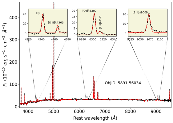
Figure 1: Optical spectrum (black colour) for one of the Seyfert 2 nuclei in our sample (see Sect. 2) obtained from the SDSS DR17. The fitting to the emission-line profiles using the ifscube code is represented in red colour. The measured emission-lines and their corresponding wavelengths are indicated. Boxes show enlargements of regions around some weak lines, as indicated.

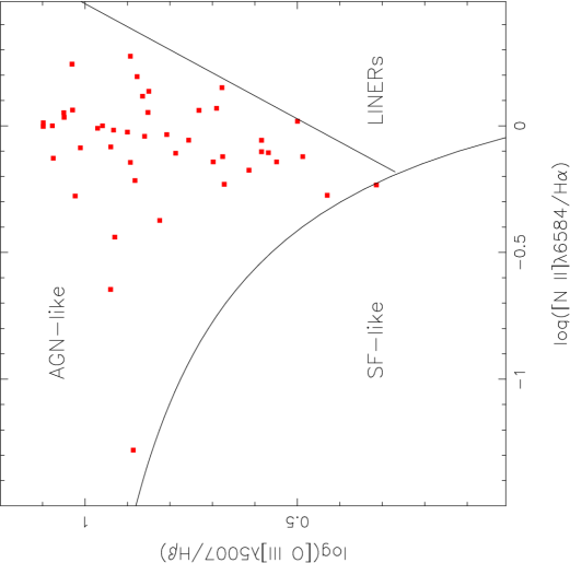
Figure 2: log([O iii]$\lambda 5007$/H$\beta$) vs. log([N ii]$\lambda 6584$/H$\alpha$]) diagnostic diagram. Red points represent the Sy 2 nuclei in our sample (see Sect. 2). The black solid curve represents the criterion (Eq. 1) proposed by Kewley et al. (2001) to separate AGN-like and SF-like objects. The black solid line represents the criterion (Eq. 2) proposed by Cid Fernandes et al. (2010) to separate AGN-like objects and LINERs.

In order to obtain a sample of Sy 2s with observational intensities of narrow (Full Width Half Maximum $<\>1000\>\rm km\>s^{-1}$) optical emission lines, we used spectroscopic data made available through the Sloan Digital Sky Survey Data Release 17, SDSS DR17 (Abdurro’uf et al., 2022). In the present study, the procedures for selection of Sy 2s, emission line measurements, reddening correction and the stellar population continuum subtraction were the same as described by Dors et al. (2022), therefore, we summarized these processes below.

For each spectrum downloaded from the SDSS DR17, we performed the extinction correction using the Cardelli et al. (1989) law assuming the parameterized extinction coefficient $R_{V}=3.1$. Thereafter, the stellar population continuum was subtracted from the spectra to obtain the pure nebular spectra using the stellar population synthesis starlight code (Cid Fernandes et al., 2005; Mateus et al., 2006; Vale Asari et al., 2016). The emission lines were fitted using the publicly available ifscube package (Ruschel-Dutra & Dall’Agnol De Oliveira, 2020; Ruschel-Dutra et al., 2021). The fluxes were corrected for extinction following the procedure described by Riffel et al. (2021b), where the observational H$\alpha$/H$\beta$ line ratio was compared with the theoretical value (H$\alpha$/H$\beta$)=2.86 proposed by Hummer & Storey (1987) for a temperature of 10 000 K and an electron density of 100 $\rm cm^{-3}$. From the resulting sample, we selected only the objects which present the [O ii]$\lambda 3726,\lambda 3729$ (hereafter [O ii]$\lambda 3727$), [O iii]$\lambda 4363$, H$\beta$, [O iii]$\lambda 5007$, H$\alpha$, [N ii]$\lambda 6584$, [S ii]$\lambda 6716,\lambda 6731$, and [S iii]$\lambda 9069$ emission-lines with a signal to noise ratio (S/N) higher than 2.0. Although the presence of the [N ii]$\lambda 5755$ and [S iii]$\lambda 6312$ auroral lines was not considered as selection criteria, when detected with (S/N) > 2 in the archival public data, their intensities were compiled.

Additionally, we also compiled from the literature emission-line intensities of Sy 2 nuclei obtained by different authors and applying the same selection criteria used for the SDSS data, with exception of the presence of the [S iii]$\lambda 9069$ line, which is not measured in most of the available data. In these cases, a cross-correlation was performed between the objects with optical data and those whose [S iii]$\lambda 9069$ was measured by Riffel et al. (2006), who presented a near-infrared (0.8-2.4 $\mu$m interval) spectral atlas of 47 AGNs. Initially, for each selected object, the [S iii]$\lambda 9069$ fluxes from Riffel et al. (2006) were divided by the Pa$\beta$ flux. Thereafter, in order to obtain the [S iii]$\lambda 9069$ in relation to H$\beta$, the (Pa$\beta$/H$\beta)=0.162$ theoretical ratio (Osterbrock, 1989) was assumed for a temperature of 10 000 K and an electron density of 100 $\rm cm^{-3}$. A similar procedure was performed by Binette et al. (2012).

Finally, for the entire sample, we applied the criterion proposed by Kewley et al. (2001)

$$\rm log([O\>III]\lambda 5007/H\beta)\>>\>\frac{0.61}{log([N\>II]\lambda 6584/H\alpha)-0.47}+1.19,$$ (1)

to separate SF-like and AGN-like objects and the criterion proposed by Cid Fernandes et al. (2010)

$$\rm log([O\>III]\lambda 5007/H\beta)\>>\>0.47+log([N\>II]\lambda 6584/H\alpha)\times 1.10,$$ (2)

to separate AGN-like and low-ionization nuclear emission-line region (LINER) objects. The final sample resulted in 45 Sy 2 nuclei, which is comprised by 33 objects from SDSS data set (redshift $z\><\>0.08$) and 12 objects from the literature (redshift $z\><\>0.04$).

The reduced number of objects (33) resulting from the SDSS database is mainly due to two selection criteria. First, the requirement for [O iii]$\lambda 4363$ measured at $\rm(S/N)\>>\>2$ makes it possible to select only 110 objects from a total of 333 Seyfert 2 nuclei. A similar sample size was obtained by Flury & Moran (2020), where the $T_{\rm e}$-method was applied in only 180 objects (see also Vaona et al. 2012; Dors et al. 2020a) selected from the SDSS DR8 (Aihara et al., 2011). Second, the requirement for the presence of both [O ii]$\lambda 3727$ and [S iii]$\lambda 9069$ reduced our sample from 110 to only 33 objects. Izotov et al. (2006), who considered the SDSS DR3 (Abazajian et al., 2005) database to estimate elemental abundances in SFs, also reported the difficulty in measuring both [O ii]$\lambda 3727$ and [S iii]$\lambda 9069$ lines, mainly for galaxies at $z\>\la\>0.02$.

In Figure 1, an example of a pure Sy 2 nebular spectrum (in black) from the SDSS sample and the fitting (in red) produced by the ifscube package are shown. In Table 5 the reddening corrected emission line intensities (in relation to H$\beta$=1.0) and the literature references from which the data were compiled are listed. In this Table, the theoretical relation $I(\lambda 9069)=0.40\times I(\lambda 9532)$ between the [S iii] emission-lines is assumed.

In Fig. 2, a log([O iii]$\lambda 5007$/H$\beta$) vs. log([N ii]$\lambda 6584$/H$\beta$) diagnostic diagram, the observational data and the above criteria (Equations 1 and 2) are shown. It can be seen that the Sy 2 sample covers a large range of ionization degree and metallicity, since a wide range of [O iii]/H$\beta$ and [N ii]/H$\alpha$ line ratio intensities are seen (e.g. Groves et al. 2006; Feltre et al. 2016; Carvalho et al. 2020).

The observational data sample is heterogeneous, in the sense that the spectra were obtained with distinct instrumentation (e.g. long-slit, fiber spectroscopy), aperture, reddening correction procedures, etc. These features could produce artificial scattering or biases in the derived abundances. Dors et al. (2020a, 2021) and Armah et al. (2021) presented a complete discussion on the use of a heterogeneous sample and its possible implications on abundance estimates. These authors pointed out that the effects of considering such a heterogeneous sample on abundance estimates produce uncertainties of $\sim 0.1$ dex, i.e. in the same order or even lower than those derived by applying the $T_{\rm e}$-method (e.g. Kennicutt et al. 2003; Hägele et al. 2008) and strong-line methods (e.g. Storchi-Bergmann et al. 1998; Denicoló et al. 2002). Moreover, Kewley et al. (2005) presented a detailed analysis of the effect of considering different apertures on the determinations of physical parameters of galaxies. These authors found that for aperture capturing less than 20 per cent of the total galaxy emission, the derived metallicity can differ by a factor of about 0.14 dex from the value obtained when the total galaxy emission is considered. However, only abundances of the nuclear regions are being considered here; therefore, the aperture effect on our estimates is not significant. Additional analysis of uncertainties in abundance estimates derived from distinct instrumentation and/or aperture has been addressed, for instance, by Mannucci et al. (2021), who analysed the Diffuse Ionized Gas (DIG) contribution to the nebular emission of SFs. These authors, specifically, found that the [S ii] line fluxes tend to be more affected in comparison with other optical line fluxes. Mannucci et al. (2021) also found that when spectra of local H ii regions are extracted using large enough apertures while still avoiding the DIG, the observed line ratios are the same as in more distant galaxies. Therefore, there should not be any bias in our sample as a result of the usage of different instruments (see also Arellano-Córdova et al. 2022; Pilyugin et al. 2022). However, the requirement for the presence of the weak [O iii]$\lambda 4363$ line (about 100 times weaker than H$\beta$) in the SDSS spectra yields a bias in our analysis, in the sense that objects with very high metallicity, where the gas suffers strong cooling and the electron temperature is low enough not to produce significant emission of this line, are mostly excluded. In fact, for instance, Dors et al. (2020a) selected from the SDSS DR7 database (Abazajian et al., 2009), 463 confirmed Sy2 spectra with only 150 objects having [O iii]$\lambda 4363$ measured with $\rm(S/N)\>>\>2$ and from these, only 36/150 have oversolar metallicity according to the $T_{\rm e}$-method applied by Dors et al. (2020b). Thus, abundance determinations obtained in the present study do not extend to objects with the highest expected metallicity (see also van Zee et al. 1998; Izotov et al. 2006; Flury & Moran 2020).

Another issue is the SF emission contribution to our AGN spectra, which can have a greater impact on the observed line fluxes for the most distant objects. Davies et al. (2014) presented a spatially resolved study of the active galaxy NGC 7130 ($z=0.016$) and found that SFs are responsible for 30 and 65 per cent of the [O iii] and H$\alpha$ luminosity, respectively. Moreover, Vidal-García et al. (2022) compared results from the NLR photoionization models (Feltre et al., 2016) incorporated into the Beagle (Bayesian SED-fitting, Chevallard & Charlot 2016) code with observational spectroscopic data and showed that the SF H$\beta$ flux contribution to the total nuclear flux of an active galaxy can range from 0 to 50 per cent. However, we emphasize that, in principle, the SF flux contribution has a minimal effect on AGN abundance estimates when a sample of objects is considered. This assertion is supported by Thomas et al. (2019), who demonstrated that the aperture effect (and consequently SF contribution) has a negligible impact on metallicity estimates once comparable mass-metallicity relations for galaxies in four redshift bins were considered.

Since the [S iii] lines of Seyfert galaxies are rarely found in the literature due to the fact that they are located in the near infrared which there are few instruments operating, it is worthwhile to compare their emission line flux ratios with those of SFs. In this regard, we consider emission line intensities of H ii galaxies (44 objects) and Giant H ii regions (GHRs, 34 objects) presented by Hägele et al. (2006, 2008); Hägele et al. (2011, 2012). Besides, we compare the Sy 2 emission lines considered in this work with those from 378 disk H ii regions located in 6 local spiral galaxies, which have been made available by the CHAOS project, and presented by Berg et al. (2015, 2020), Croxall et al. (2015, 2016), and Rogers et al. (2021, 2022). This comparison (see also Díaz & Zamora 2022) is shown in Fig. 3. A clear correlation is derived between the two dataset since both line ratios are dependent on the ionization degree of the gas. Interestingly, Sy 2 nuclei present similar [S iii]/[S ii] line ratio intensities to those of SFs. The Sy 2 [O iii]/[O ii] line ratio intensities are in consonance with those of H ii galaxies and GHRs and are higher than those from disk H ii regions.

Figure 3: Logarithm of [O iii]$\lambda 5007$/[O ii]$\lambda 3727$ versus [S iii]$\lambda 9069+\lambda 9532$/[S ii]$\lambda 6716+\lambda 6731$. Red points represent the Sy 2 sample (see Sect. 2) whose emission line intensities are listed in Table 5. Black points represent disk H ii regions whose data were taken from the chaos project and obtained by Berg et al. (2015, 2020), Croxall et al. (2015, 2016) and Rogers et al. (2021, 2022). Blue points represent H ii galaxies taken from Hägele et al. (2006, 2008); Hägele et al. (2011, 2012) and pink points represent GHRs taken from Hägele et al. (2006).

3 Abundance estimates

Table 1: Atomic dataset used for collisionally excited lines of selected element ions.

Ion	Transition probabilities	Collisional strengths
S+	Froese Fischer et al. (2006)	Tayal & Zatsarinny (2010)
S2+	Froese Fischer et al. (2006)	Tayal & Gupta (1999)
O+	Wiese et al. (1996)	Kisielius et al. (2009)
O2+	Froese Fischer & Tachiev (2004), Storey & Zeippen (2000)	Storey et al. (2014)

Table 2: Estimates of $T_{\rm e}(\rm O^{2+})$, $T_{\rm e}(\rm N^{+})$ and $T_{\rm e}(\rm S^{2+})$ used to obtain the relations given by Eqs. 3 and 4. The line ratios are: $RO3={{\color[rgb]{0,0,1}(}}[\text{O\,{iii}}]\lambda 4959+\lambda 5007)/\lambda 4363$, $RN2={{\color[rgb]{0,0,1}(}}[\text{N\,{ii}}]\lambda 6548+\lambda 6584)/\lambda 5755$, $RS3={{\color[rgb]{0,0,1}(}}[\text{S\,{iii}}]\lambda 9069+\lambda 9532)/\lambda 6312$ and $RS2=[\text{S\,{ii}}]\lambda 6716/\lambda 6731$.

Object	$RO3$	$RN2$	$RS3$	$RS2$	$T_{\rm e}$($\rm O^{2+}$)[K]	$T_{\rm e}$($\rm N^{+}$)[K]	$T_{\rm e}$($\rm S^{2+}$)[K]	$N_{\rm e}[\rm cm^{-3}]$	Ref.
IZw 92	42.62 $\pm$ 8.52	66.50 $\pm$ 13.30	—	0.92 $\pm$ 0.09	16350 $\pm$ 1646	9929 $\pm$ 788	—	1176 $\pm$ 427	1
Mrk 3	69.41 $\pm$ 13.88	87.29 $\pm$ 17.45	—	0.89 $\pm$ 0.08	13151 $\pm$ 1059	8969 $\pm$ 638	—	1221 $\pm$ 395	2
Mrk 78	112.90 $\pm$ 22.58	95.31 $\pm$ 19.06	—	1.11 $\pm$ 0.11	11023 $\pm$ 743	8754 $\pm$ 607	—	467 $\pm$ 229	2
Mrk 34	100.90 $\pm$ 20.18	87.27 $\pm$ 17.45	—	1.02 $\pm$ 0.10	11445 $\pm$ 800	9012 $\pm$ 643	—	691 $\pm$ 280	2
Mrk 1	69.09 $\pm$ 13.81	135.45 $\pm$ 27.09	—	0.94 $\pm$ 0.09	13187 $\pm$ 1060	7773 $\pm$ 481	—	1000 $\pm$ 362	2
Mrk 533	95.00 $\pm$ 19.00	240.00 $\pm$ 48.00	—	0.86 $\pm$ 0.08	11681 $\pm$ 834	6591 $\pm$ 346	—	1319 $\pm$ 429	3
Mrk 612	60.00 $\pm$ 12.00	112.00 $\pm$ 22.40	—	1.36 $\pm$ 0.13	13993 $\pm$ 1199	8304 $\pm$ 551	—	87 :	3
ESO 138 G1	34.23 $\pm$ 6.84	47.73 $\pm$ 9.54	—	0.97 $\pm$ 0.09	18386 $\pm$ 2084	11457 $\pm$ 1055	—	1003 $\pm$ 366	4
NGC 2992	40.36 $\pm$ 8.07	98.20 $\pm$ 19.64	—	1.12 $\pm$ 0.11	16831 $\pm$ 1736	8659 $\pm$ 595	—	514 $\pm$ 266	5
NGC 2210	24.36 $\pm$ 4.87	117.77 $\pm$ 23.55	—	1.06 $\pm$ 0.10	22797 $\pm$ 3095	8143 $\pm$ 527	—	744 $\pm$ 328	5
NGC 5506	73.57 $\pm$ 14.70	168.50 $\pm$ 33.70	—	0.92 $\pm$ 0.09	12859 $\pm$ 1012	7279 $\pm$ 421	—	1074 $\pm$ 386	5
Mrk 348	23.7 $\pm$ 2.4	31.8 $\pm$ 11.9		0.83 $\pm$ 0.03	28600 $\pm$ 4700	21700 $\pm$ 6100	—	1940 $\pm$ 245	6
Mrk 607	29.7 $\pm$ 10.2	80.6 $\pm$ 16.2		0.87 $\pm$ 0.11	23500 $\pm$ 2700	10200 $\pm$ 1300	—	1548 $\pm$ 707	6
56067-0382	41.43 $\pm$ 8.29	12.29 $\pm$ 2.46	—	1.06 $\pm$ 0.16	16604 $\pm$ 1694	31367 $\pm$ 8555	—	669 $\pm$ 463	7
55539-0167	82.20 $\pm$ 16.44	24.49 $\pm$ 4.90	—	1.13 $\pm$ 0.17	12334 $\pm$ 928	16655 $\pm$ 2244	—	442 $\pm$ 349	7
56001-0293	109.00 $\pm$ 21.80	37.02 $\pm$ 7.40	—	1.39 $\pm$ 0.21	11159 $\pm$ 760	13147 $\pm$ 1393	—	58 :	7
55742-0383	99.80 $\pm$ 19.96	42.04 $\pm$ 8.41	—	1.13 $\pm$ 0.17	11497 $\pm$ 806	12245 $\pm$ 1202	—	432 $\pm$ 340	7
55302-0655	41.20 $\pm$ 8.24	47.71 $\pm$ 9.54	—	1.24 $\pm$ 0.19	16672 $\pm$ 1708	11537 $\pm$ 1068	—	266 $\pm$ 0	7
56568-0076	105.33 $\pm$ 21.07	96.13 $\pm$ 19.23	—	1.03 $\pm$ 0.15	11280 $\pm$ 780	8715 $\pm$ 604	—	660 $\pm$ 407	7
56566-0794	94.80 $\pm$ 18.96	127.06 $\pm$ 25.41	4.36 $\pm$ 0.87	1.18 $\pm$ 0.18	11713 $\pm$ 838	7968 $\pm$ 505	21665 $\pm$ 3991	342 :	7
55181-0154	130.33 $\pm$ 26.07	—	3.85 $\pm$ 0.77	0.98 $\pm$ 0.15	10508 $\pm$ 675	—	24380 $\pm$ 5015	786 $\pm$ 474	7
56088-0473	128.33 $\pm$ 25.67	—	18.00 $\pm$ 3.60	1.09 $\pm$ 0.16	10566 $\pm$ 682	—	9244 $\pm$ 747	502 $\pm$ 349	7
56034-0154	84.86 $\pm$ 16.97	—	12.00 $\pm$ 2.40	1.09 $\pm$ 0.16	12184 $\pm$ 909	—	11052 $\pm$ 1070	527 $\pm$ 370	7
56626-0636	102.00 $\pm$ 20.40	—	3.49 $\pm$ 0.70	1.08 $\pm$ 0.16	11409 $\pm$ 795	—	27079 $\pm$ 6116	537 $\pm$ 371	7
55651-0052	177.00 $\pm$ 35.40	—	5.37 $\pm$ 1.07	1.06 $\pm$ 0.16	9576 $\pm$ 560	—	18131 $\pm$ 2884	549 $\pm$ 368	7
56206-0454	74.11 $\pm$ 14.82	—	6.17 $\pm$ 1.23	1.23 $\pm$ 0.18	12842 $\pm$ 1010	—	16315 $\pm$ 2354	267 :	7
55860-0112	71.09 $\pm$ 14.22	—	3.39 $\pm$ 0.68	1.02 $\pm$ 0.15	13038 $\pm$ 1038	—	27975 $\pm$ 6506	724 $\pm$ 448	7
55710-0116	107.71 $\pm$ 21.54	—	12.29 $\pm$ 2.46	0.92 $\pm$ 0.14	11189 $\pm$ 764	—	10917 $\pm$ 1047	1018 $\pm$ 578	7
56366-0928	47.50 $\pm$ 9.50	—	3.14 $\pm$ 0.63	1.00 $\pm$ 0.15	15523 $\pm$ 1474	—	30648 $\pm$ 7717	834 $\pm$ 517	7
56328-0550	81.67 $\pm$ 16.33	—	7.48 $\pm$ 1.50	1.28 $\pm$ 0.19	12373 $\pm$ 934	—	14339 $\pm$ 1821	190 :	7
55617-0758	76.80 $\pm$ 15.36	—	3.45 $\pm$ 0.69	0.90 $\pm$ 0.13	12640 $\pm$ 978	—	27394 $\pm$ 6222	1156 $\pm$ 609	7
56003-0218	67.14 $\pm$ 13.43	—	5.89 $\pm$ 1.18	0.97 $\pm$ 0.14	13337 $\pm$ 1088	—	16867 $\pm$ 2531	889 $\pm$ 504	7
55505-0654	198.75 $\pm$ 39.75	—	12.00 $\pm$ 2.40	1.12 $\pm$ 0.17	9268 $\pm$ 524	—	11052 $\pm$ 1072	422 $\pm$ 319	7

References: (1) Kraemer et al. (1994), (2) Koski (1978), (3) Shuder & Osterbrock (1981), (4) Alloin et al. (1992), (5) Shuder (1980), (6), Riffel et al. (2021a), (7) SDSS sample.

For the Sy 2 sample previously described, we determined the sulphur and oxygen abundances relative to hydrogen. To do that, electron temperatures representing the zones where distinct ions are located in the gas phase, electron density and ionic abundances were calculated using the 1.1.13 version of PyNeb code (Luridiana et al., 2015), which permits an interactive procedure in the derivation of these parameters. The references for the predefined atomic parameters incorporated into the PyNeb code are listed in Table 1.

As the line measurements for some objects (9/45) of our sample does not present observational errors, the abundance uncertainties were estimated using Monte Carlo simulations. For each diagnostic line, we generate 1000 random values assuming a Gaussian distribution with a standard deviation equal to the associated uncertainty of 10 % and 20 % for strong (e.g. [O iii]$\lambda 5007$) and auroral (e.g. [O iii]$\lambda 4363$) line intensities involved in the diagnostics, respectively. Thereafter, an empirical Ionization Correction Factor (ICF) was considered in the derivation of the total sulphur abundance. For objects that have measured emission-line errors (36/45), the uncertainties in the final abundance values were obtained propagating the errors in the line measurements, electron temperature and electron density. Subsequently, the description of the employed methodology is presented.

3.1 Temperature estimations

Several studies have been directed to estimate the chemical composition of SFs and, in almost all of these estimates, it has been a common practice to use temperature relations derived from photoionization models to infer the temperatures in the unobserved ionization zones (e.g. Stasińska 1990; Garnett 1992; Pérez-Montero & Díaz 2003; Izotov et al. 2006). However, when temperature relations predicted by photoionization models simulating SFs are compared with direct estimates relying on auroral lines, large deviations are found, reaching up to $\sim 5000$ K (e.g. Hägele et al. 2008; Berg et al. 2020; Arellano-Córdova & Rodríguez 2020). Despite the fact that temperature relations for AGNs are barely found in the literature (see Dors et al. 2020b; Armah et al. 2021; Monteiro & Dors 2021), it seems that similar disagreement is also derived for this class of object. In fact, Riffel et al. (2021a) compared the $T_{\rm e}(\rm N^{+})$-$T_{\rm e}(\rm O^{2+})$ relation predicted by photoionization models, built using the cloudy code (Ferland et al., 2013), with values derived from observational auroral emission lines for a sample of 12 local Seyfert nuclei. The model predictions reproduce the direct temperature observations for all objects, except for Mrk 348 for which the direct $T_{\rm e}(\rm N^{+})$ value is $\sim$10 000 K higher than the predicted one. This object is know to host ionized gas outflows (Freitas et al., 2018) and probably the higher observed temperatures are due to extra heating caused by shocks (see Dors et al. 2021), which is not accounted in the photoionization models considered by Riffel et al. (2021a). Obviously, additional comparison with a larger sample of objects combined with kinematic studies (e.g. Xu et al. 2021; Flury et al. 2022, in preparation) of objects where gas outflow is detected, is necessary to confirm this result.

Since comparisons between observational emission line intensities and the ones predicted by photoionization models indicate that the main ionization source of most NLR of Sy 2s is the radiation emitted by gas accretion into a supermassive black hole, for objects in the local universe (see e.g. Stasińska 1984; Ferland & Osterbrock 1986; Storchi-Bergmann et al. 1998; Groves et al. 2006; Feltre et al. 2016; Castro et al. 2017; Dors et al. 2017; Dors et al. 2020b; Pérez-Montero et al. 2019; Thomas et al. 2019; Carvalho et al. 2020; Armah et al. 2021) and also at high redshift (see e.g. Nagao et al. 2006; Matsuoka et al. 2009; Matsuoka et al. 2018; Dors et al. 2014; Dors et al. 2018; Dors et al. 2019; Nakajima et al. 2018; Mignoli et al. 2019; Guo et al. 2020), we are able to apply the $T_{\rm e}$-method to derive reliable estimates. However, the weak temperature-sensitive auroral emission-line measurements are barely available in the literature for AGNs, therefore we developed our own empirical method based on our sample.

To derive the empirical relations for our abundance estimates, we used auroral line intensities from our sample and those of Sy 2 NLRs available in the literature. Firstly, the observational intensities of the $RO3$=[O iii]($\lambda 4959+\lambda 5007$)/$\lambda 4363$ and $RN2$=[N ii]($\lambda 6548+\lambda 6584$)/$\lambda 5755$ line ratios were used to calculate $T_{\rm e}(\rm O^{2+})$ and $T_{\rm e}(\rm N^{+})$, respectively, for 18 objects, i.e. 7 objects of our sample (see Table 5) and 11 Sy 2 compiled by Dors et al. (2020b). To derive $T_{\rm e}(\rm S^{2+})$, we used the $RS3$=[S iii]($\lambda 9069+\lambda 9532$)/$\lambda 6312$ line ratios for 14 objects (over 45) in our sample (see Table 5). For each object, the temperature estimates were performed assuming a constant electron density ($N_{\rm e}$) value across the nebula, which is derived from the $RS2$=[S ii]$\lambda 6716/\lambda 6731$ intensity ratio. In Table 2, the objects and their corresponding $RO3$, $RN2$, $RS3$ and $RS2$ line intensities ratios, the electron density, $T_{\rm e}(\rm O^{2+})$, $T_{\rm e}(\rm N^{+})$ and $T_{\rm e}(\rm S^{2+})$ temperature derived values are listed. We note that the object 56067-0382 has a $T_{\rm e}(\rm N^{+})$ higher than those derived for other objects and similar to the value derived for Mrk 348 by Riffel et al. (2021a). Probably 56067-0382 presents gas outflows but its temperatures were still considered. Since in most cases only the [O iii]$\lambda 4363$ auroral line is measured (e.g. van Zee et al. 1998; Kennicutt et al. 2003), we proposed, as usual, temperature relations with respect to $T_{\rm e}(\rm O^{2+})$. In Fig. 4, $T_{\rm e}(\rm N^{+})$ and $T_{\rm e}(\rm S^{2+})$ are plotted against $T_{\rm e}(\rm O^{2+})$, with the values in units of $10^{4}$ K. In the upper panel of this figure, the dashed line represents the equality between $T_{\rm e}(\rm S^{2+})$ and $T_{\rm e}(\rm O^{2+})$. As for SFs (e.g., see Hägele et al. 2008; Berg et al. 2020), clear correlations between the Sy 2 temperatures are observed, with a linear regression resulting in

$$t_{\mathrm{e}}(\mathrm{N^{+}})=0.36(\pm 0.23)\times t_{\mathrm{e}}(\mathrm{O^{2+}})+{\rm 0.55(\pm 0.39)},$$ (3)

and

$$t_{\mathrm{e}}(\mathrm{S^{2+}})=2.23(\pm 1.12)\times t_{\mathrm{e}}(\mathrm{O^{2+}})-{\rm 0.74(\pm 1.34)},$$ (4)

where $t_{\rm e}=T_{\rm e}/10^{4}\>\rm K$.

It can be seen in Fig. 4 that higher temperature values for $\rm S^{2+}$ are derived in comparison with those for $\rm O^{2+}$, probably indicating that the former ion occupy an inner gas region than the latter. Conversely, an opposite result is derived for disk H ii regions, i.e. $T_{\rm e}(\rm O^{2+})$ is $\sim 1000$ K higher than $T_{\rm e}(\rm S^{2+})$ (e.g. Rogers et al. 2021). Hägele et al. (2006) analysed the relation between $T_{\rm e}(\rm O^{2+})$ and $T_{\rm e}(\rm S^{2+})$ using a sample that comprises H ii galaxies, giant extragalactic H ii regions, Galactic H ii regions, and H ii regions from the Magellanic Clouds (MCs). These authors found that the [S iii] electron temperatures are higher than the corresponding [O iii] estimations for most objects presenting temperatures higher than about 14 000K, mainly the metal poor H ii galaxies, and the opposite behaviour for the coolest nebulae, mainly giant extragalactic H ii regions, Galactic H ii regions, and H ii regions from the MCs, which present the highest metallicities. Taking into account the temperatures of the different samples studied by Hägele et al. (2008, H ii galaxies that present the higher temperatures) and Rogers et al. (2021, galactic disk H ii regions with lower temperatures), the $T_{\rm e}(\rm S^{2+})$-$T_{\rm e}(\rm O^{2+})$ behavior derived in the present paper for Sy 2s is the same as found by Hägele et al. (2006).

Table 3: Critical densities for collisional de-excitation for the lines involved in the present work. Values were calculated with the PyNeb code (Luridiana et al., 2015) assuming an electron temperature of 15 000 K.

Line	$N_{\rm c}$ ($\rm cm^{-3})$
$[\text{O\,{ii}}]\lambda 3726$	$4.72\times 10^{3}$
$[\text{O\,{ii}}]\lambda 3729$	$1.49\times 10^{3}$
$[\text{O\,{iii}}]\lambda 4363$	$2.88\times 10^{7}$
$[\text{O\,{iii}}]\lambda 5007$	$7.83\times 10^{5}$
$[\text{N\,{ii}}]\lambda 5755$	$1.87\times 10^{7}$
$[\text{S\,{iii}}]\lambda 6312$	$1.44\times 10^{7}$
$[\text{N\,{ii}}]\lambda 6484$	$1.04\times 10^{5}$
$[\text{S\,{ii}}]\lambda 6716$	$1.37\times 10^{3}$
$[\text{S\,{ii}}]\lambda 6731$	$3.67\times 10^{3}$
$[\text{S\,{iii}}]\lambda 9069$	$6.42\times 10^{5}$

Spatially resolved observational studies of NLRs have found a profile of electron density along the AGN radius, in the sense that denser gas is located in the inner regions. For instance, Freitas et al. (2018), who obtained emission-line flux of two-dimensional maps from five bright nearby Seyfert nuclei, obtained electron densities ranging from $\sim 2500\>\rm cm^{-3}$ in the central parts to $\sim 100\>\rm cm^{-3}$ in the outskirts (see also Revalski et al. 2018a; Revalski et al. 2018b, 2021, 2022; Kakkad et al. 2018; Mingozzi et al. 2019; Ruschel-Dutra et al. 2021). Moreover, electron density estimations through the [Ar iv]$\lambda 4711/\lambda 4740$ line ratio, which traces the density in the innermost layers, showed values of up to $\sim$13 000 $\rm cm^{-3}$ (e.g. Congiu et al. 2017; Cerqueira-Campos et al. 2021). Thus, density values derived from [S ii] lines may not be representative of the region where $\rm S^{2+}$ ions are located, which could inherently introduce an error in the $T_{\rm e}(\rm S^{2+})$ values. In order to explore the influence of the electron density on the sulphur temperature estimations, we show in Fig. 5 the $t_{\rm e}(\rm S^{2+})$ derived assuming the $N_{\rm e}$ values from [S ii]$\lambda 6716/\lambda 6731$ line ratios (listed in Table 2) versus the estimations considering a fixed value of 13 000 $\rm cm^{-3}$, as derived by Congiu et al. (2017) for the extended narrow-line region of the Seyfert 2 galaxy IC 5063. We notice a good agreement between the values, with a difference of $\sim 2\,\%$, which is lower than the uncertainty produced by the error in the line measurements ($\sim 10\%$, see Table 2). In Table 3 the critical density ($N_{\rm c}$) values for the lines involved in the present work, calculated with the PyNeb code (Luridiana et al., 2015) assuming an electron temperature of 15 000 K, are listed. One can see that $N_{\rm c}$ values are higher than the electron density values (listed in Table 6) derived for our Sy 2 sample. Thus, electron density variations in NLRs have a minimal influence on our temperature estimates. For some objects, the emission-line errors are significant, thus frequently with density error bars larger than the determinations themselves. Therefore we use “:” to indicate that error bars are at least an order of magnitude larger than the expected density (see Table 6).

Due to the similarity among the $\rm S^{+}$, $\rm N^{+}$ and $\rm O^{+}$ ionization potentials (23.33 eV, 29.60 eV and 35.12 eV, respectively) and because the [S ii]$\lambda\lambda 4068,4076$ and [O ii]$\lambda\lambda 7320,7330$ auroral lines are not measured in our sample of spectra, as in Rogers et al. (2021), we adopted $T_{\rm e}(\rm S^{+})$=$T_{\rm e}(\rm O^{+})$=$T_{\rm e}(\rm N^{+})$. In objects for which it is possible to estimate directly $T_{\rm e}(\rm N^{+})$ (7/45) and $T_{\rm e}(\rm S^{2+})$ (14/45), these temperatures were assumed as representative of the low and high ionization zones, respectively. Otherwise, when the [N ii]$\lambda 5755$ and [S iii]$\lambda 6312$ auroral emission-line measurements are not available, $T_{\rm e}(\rm N^{+})$ and $T_{\rm e}(\rm S^{2+})$ were derived from the Eqs. 3 and 4, respectively. In Table 6, electron density and temperature values for the objects in our sample are presented.

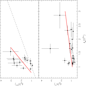
Figure 4: Comparing direct temperature values for different ions. Values are in units of $10^{4}$ K. Botton panel: $t_{\rm e}(\rm O^{2+})$ and $t_{\rm e}(\rm N^{+})$ are derived through the $RO3$=[O iii]($\lambda 4959+\lambda 5007$)/$\lambda 4363$ and $RN2$=[N ii]($\lambda 6548+\lambda 6584$)/$\lambda 5755$ line intensities ratios, respectively, and the electron density (from the $RS2$=[S ii]$\lambda 6716/\lambda 6731$) listed in Table 2, and by using version 1.1.13 of PyNeb code (Luridiana et al., 2015). The red line represents the linear regression to the points given by Eq. 3. Top panel: same as bottom panel but for $t_{\rm e}(\rm S^{2+})$ values derived from $RS3$=[S iii]($\lambda 9069+\lambda 9532$)/$\lambda 6312$. Red line represents the linear regression to the points given by Eq. 4 while the dashed line the equality between the estimates.

Figure 5: Comparison between electron temperatures (in units of $10^{4}$ K) derived from the $RS3$=[S iii]($\lambda 9069+\lambda 9532$)/$\lambda 6312$ assuming electron density estimations via the $RS2$=[S ii]$\lambda 6716/\lambda 6731$ (listed in Table 2) with the estimates assuming a value of $13\,000\,{\rm cm^{-3}}$ as derived by Congiu et al. (2017) from [Ar iv]$\lambda 4711/\lambda 4740$. Line represents the equality between the two estimates.

3.2 Abundance derivation

For each object of our sample, using the emission line intensity ratios listed in Table 5, the electron temperature and electron density values (listed in Table 6) as well as the PyNeb code (Luridiana et al., 2015), we derived the sulphur ($\rm S^{+}$, $\rm S^{2+}$) and oxygen ($\rm O^{+}$, $\rm O^{2+}$) ionic abundances. Afterwards, applying an empirical ICF for the sulphur and a typical value for the oxygen ICF, the total abundances for the S/H and O/H were estimated. In what follows, we describe the methodology employed in the derivation of the abundance of each considered element.

3.2.1 Oxygen abundance

The total oxygen abundance in relation to the hydrogen one was derived assuming

$${\rm\frac{O}{H}=ICF(O^{+}+O^{2+})\>\times\>\left[\frac{O^{+}}{H^{+}}+\frac{O^{2+}}{H^{+}}\right],}$$ (5)

where ICF($\rm O^{+}+O^{2+}$) represents the Ionization Correction Factor for oxygen which takes into account the contribution of unobservable oxygen ions, whose emission lines are observed in other spectral bands such as X-rays (e.g. Cardaci et al. 2009, 2011; Bianchi et al. 2010; Bogdán et al. 2017; Maksym et al. 2019; Kraemer et al. 2020) and IR (e.g. Diamond-Stanic & Rieke 2012; Fernández-Ontiveros et al. 2016). The $\rm O^{2+}/H^{+}$ ionic abundance was calculated by using the [O iii]$\lambda 5007/\rm H\beta$ line ratio and assuming the direct $T_{\rm e}(\rm O^{2+})$ and $N_{\rm e}$ values derived from $RO3$ and $RS2$, respectively. The $\rm O^{+}/H^{+}$ abundance was calculated from the [O ii]$\lambda 3727/\rm H\beta$ emission line ratio and assuming $T_{\rm e}(\rm O^{+})$=$T_{\rm e}(\rm N^{+})$ with $T_{\rm e}(\rm N^{+})$ estimated from the empirical relation given by Eq. 3 when the [N ii]$\lambda 5755$ auroral emission-line measurement is not available.

To derive ICF($\rm O^{+}+O^{2+}$) it is necessary to calculate the $\rm He^{+}/H^{+}$ and $\rm He^{2+}/H^{+}$ ionic abundances (e.g. Torres-Peimbert & Peimbert 1977; Izotov et al. 2006; Flury & Moran 2020), which is not possible because in most of the AGN spectra from our sample, the helium recombination line $\lambda 4686\>\textup{\AA}$ is not measured. Therefore, for consistency, the ICF($\rm O^{+}+O^{2+}$) is assumed to have a value of 1.50 for all objects, which is an average value derived by Dors et al. (2022), who found ICF values ranging from 1.30 to 1.70 for a sample of 65 local ($z\>\la\>0.2$) Sy 2s. This ICF value translates into an abundance correction of $\sim 0.2$ dex, i.e., somewhat higher than the uncertainty ($\sim 0.1$ dex) of abundances usually relied on for the $T_{\rm e}$-method (e.g. Kennicutt et al. 2003; Hägele et al. 2008).

3.2.2 Sulphur abundance

The $\rm S^{+}/H^{+}$ ionic abundance for each object of our sample was derived by using the [S ii]$(\lambda 6716+\lambda 6731)/\rm H\beta$ line intensities ratio and assuming $T_{\rm e}$($\rm S^{+}$)=$T_{\rm e}$($\rm N^{+}$), where $T_{\rm e}$($\rm N^{+}$) was calculated from Eq. 3 when the [N ii]$\lambda 5755$ auroral emission-line measurement is not available. Due to the similarity between the ionization potentials of $\rm S^{+}$ and $\rm N^{+}$ (23.33 eV and 29.60 eV, respectively) these ions are approximately located in the same gas region and the use of a common temperature for both is a good approach as largely used in SF chemical abundance studies (e.g. Kennicutt et al. 2003). However, Rogers et al. (2021), who compared SF direct estimates of $T_{\rm e}(\rm S^{+})$ [derived from $RAS2$=[S ii]$(\lambda 6716+\lambda 6731)/(\lambda 4068+\lambda 4074)$] with $T_{\rm e}(\rm N^{+})$ [derived from $RN2$=[N ii]$(\lambda 6548+\lambda 6584)/(\lambda 5755)$], found somewhat higher $T_{\rm e}(\rm S^{+})$ values than $T_{\rm e}(\rm N^{+})$, with an intrinsic dispersion of $\sim 950$ K between these temperatures. Unfortunately, $RAS2$ values for Sy 2 are rarely found in the literature thus far, which makes it impossible to verify whether any of these conclusions also apply to AGNs.

Similarly, the $\rm S^{2+}/H^{+}$ was derived by using the [S iii]$\lambda 9069/\rm H\beta$ line intensities ratio listed in Table 5 and the $T_{\rm e}(\rm S^{2+})$ values from Eq. 4 when the $RS3$ line ratio is not available. The uncertainties associated with the sulphur ionic estimates is mainly due to the error in the measurements of the emission-line fluxes and the uncertainties in the temperature values. In Table 7, the sulphur ionic abundance values for each object of the sample are listed.

The total sulphur abundance in relation to the hydrogen one was considered to be

$${\rm\frac{S}{H}=ICF(S^{+}+S^{2+})\>\times\>\left[\frac{S^{+}}{H^{+}}+\frac{S^{2+}}{H^{+}}\right]},$$ (6)

where ICF($\rm S^{+}+S^{2+}$) is the Ionization Correction Factor for sulphur. Since AGNs have harder ionizing sources than typical SFs (e.g. Feltre et al. 2016), it is expected that the gas phase of these objects contains the presence of ions with higher ionization level than $\rm S^{2+}$. In fact, [S viii]$\lambda 9910$ and [S ix]$\lambda 12520$ emission lines were observed in large number of AGNs in the sample presented by Riffel et al. (2006). However, measurements of $\rm S^{3+}$ lines (e.g. [S iv]$10.51\micron$) are not available in the literature, which makes it impossible for the derivation of an empirical ICF(S) for AGNs, such as derived for SFs by Dors et al. (2016).

The first ICF for sulphur (likewise for other elements) was proposed for SFs by Peimbert & Costero (1969) and it is given by

$$\rm ICF(S^{+}+S^{2+})=\frac{\rm S^{+}+S^{2+}}{\rm S^{+}}=\frac{\rm O^{+}+O^{2+}}{\rm O^{+}}.$$ (7)

Rogers et al. (2021) tested the application of this ICF for SFs (see also Díaz & Zamora 2022) and pointed out that it is particularly reliable for low ionization degree, i.e. when $\rm O^{+}$ zone is more dominant than the $\rm O^{2+}$ zone [$(\rm O^{+}/O)\>>\>0.6$]. Hitherto, there has not been sulphur ICFs for AGNs in the literature and it is unknown if the above relation is completely valid for this object class. Therefore, in order to ascertain whether the sulphur ICF can be applied to Sy 2s, we performed a simple test to verify the equality indicated in Eq. 7. The ionic ratios for our sample are plotted in Fig. 6, where the black solid line represents the equality between the estimates, while the dashed lines represent the deviations of $20\,\%$ from the one-one relation. It can be seen that, despite the scattering, most of the ionic abundance ratio estimates are located around of the one-one relation. Thus, we assumed as valid the Eq. 7 for NLR sulphur abundance estimates.

Figure 6: Sulphur versus oxygen ionic abundance ratios for our sample of objects (see Sect. 2) calculated via the $T_{\rm e}$-method (see Sect. 3). Solid line represents the equality between the estimates. Dashed lines correspond to the deviation of $20\,\%$ from the one-one relation representing the mean error in the ionic abundance estimations.

Ionic and total oxygen and sulphur abundance estimates derived through the $T_{\rm e}$-method together with the sulphur ICFs for each object in our sample are listed in Table 7.

4 Results & Discussion

4.1 Temperature estimates

Recent studies of spatially resolved central parts of galaxies have uncovered the temperature structure of a few AGNs. For instance, Revalski et al. (2021), using Hubble Space Telescope and Apache Point Observatory spectroscopy, obtained direct estimates of $T_{\rm e}(\rm O^{2+})$ along the radius of the Sy 2 nucleus of Mrk 78 and found temperatures in the range 10 000-15 000 K, with no systematic variation (see also Revalski et al. 2018a; Revalski et al. 2018b). Riffel et al. (2021c) used Gemini GMOS-IFU observations of three luminous nearby Seyfert galaxies (Mrk 79, Mrk 348 and Mrk 607) and estimated $T_{\rm e}(\rm O^{2+}$) fluctuations in the inner 0.4–1.1 kpc region of these galaxies. These authors found temperature fluctuations similar to those derived in SFs and PNe. Despite the revelations provided by these recent studies, an advance in the understanding of the temperature structure of AGNs, additional point-to-point or integrated $T_{\rm e}$ estimates through distinct emission lines [e.g. [S iii]$(\lambda 9069+\lambda 9532)/\lambda 6312$ and [N ii]$(\lambda 6548+\lambda 6584)/\lambda 5755$] are rare in the literature, prompting further investigation of the AGN temperature structure. Thus, our temperature estimates provide valuable knowledge to the nature of NLRs.

A large number of AGNs present gas outflows (e.g. Riffel et al. 2020; Armus et al. 2022), shocks (e.g. Aldrovandi & Contini 1984; Dopita & Sutherland 1995; Dors et al. 2021) and neutral gas reservoirs which can coexist with the ionized gas (e.g. García-Burillo et al. 2014) and, in combination with the hard ionization source (e.g. Feltre et al. 2016), trend to produce a more complex gas structure than that of SFs (e.g. Hägele et al. 2006; García-Benito et al. 2010; Pérez-Montero et al. 2011; Monreal-Ibero et al. 2012; Durré & Mould 2018). However, complex temperature structures can also be observed in SFs (e.g., Dopita et al. 2005; Jin et al. 2022) produced, for instance, by starburst-driven outflows cooling (e.g. Danehkar et al. 2022). On the scenario where distinct physical processes drive the gas structure, it is expected that temperature relations of AGNs tend to differ from the ones derived for SFs. In order to test this hypothesis, in Fig. 7, we compare our Sy 2 temperature estimates and empirical relations (Eqs. 3 and 4) with those derived for SFs by the following authors:

1. Hägele et al. (2006): these authors used their own high quality spectra of H ii galaxies and a large literature compilation of H ii galaxies, Giant Extragalactic H ii regions (GHRs), Galactic H ii regions, and H ii regions from the Magellanic Clouds performed by Pérez-Montero et al. (2006) to analyse the relation between $T_{\rm e}(\rm O^{2+})$ and $T_{\rm e}(\rm S^{2+})$ values derived using the $T_{\rm e}$-method (see Fig. 7 of Hägele and collaborators). Their linear fitting to the complete sample gave the relation:

   $$t_{\mathrm{e}}(\mathrm{S^{2+}})=1.19(\pm 0.08)\times t_{\mathrm{e}}(\mathrm{O^{2+}})-{\rm 0.32(\pm 0.10)},$$ (8)

   which has a validity range of $0.70\>\lessapprox\>t_{\mathrm{e}}(\mathrm{O^{2+}})\>\lessapprox\>2.0$.

2. Rogers et al. (2021): the estimates by these authors include temperature values obtained for a large number of disk H ii regions in the spiral galaxy NGC 2403 using the $T_{\rm e}$-method. These estimates combined with those of H ii regions in four spiral galaxies (see Fig. 3 by Rogers et al. 2021) resulted in the relations:

   $$t_{\mathrm{e}}(\mathrm{N^{+}})=0.79(\pm 0.14)\times t_{\mathrm{e}}(\mathrm{O^{2+}})+{\rm 0.16(\pm 0.13)},$$ (9)

   and

   $$t_{\mathrm{e}}(\mathrm{S^{2+}})=1.58(\pm 0.17)\times t_{\mathrm{e}}(\mathrm{O^{2+}})-{\rm 0.57(\pm 0.16)},$$ (10)

   which are valid for $0.70\>\lessapprox\>t_{\mathrm{e}}(\mathrm{O^{2+}})\>\lessapprox\>1.5$.

3. Arellano-Córdova & Rodríguez (2020): these authors compiled emission line intensities of H ii regions from the literature to explore the behaviour of the $T_{\rm e}(\rm N^{+})$-$T_{\rm e}(\rm O^{2+})$ temperature relation. These authors found that this relation has a dependence on the gas ionization degree, which is traced by the line ratio $P=([\text{O\,{iii}}]\lambda 4959+\lambda 5007)/[\text{O\,{ii}}]\lambda 3727+[\text{O\,{iii}}]\lambda 4959+\lambda 5007$. The following relations, which hold for $0.60\>\lessapprox\>t_{\mathrm{e}}(\mathrm{O^{2+}})\>\lessapprox\>1.7$, were derived:
   For $P\><\>0.5$

   $$\frac{1}{t_{\mathrm{e}}(\mathrm{N^{+}})}=\frac{0.54(\pm 0.05)}{t_{\mathrm{e}}(\mathrm{O^{2+}})}+0.52(\pm 0.08)$$ (11)

   and for $P\>>\>0.5$

   $$\frac{1}{t_{\mathrm{e}}(\mathrm{N^{+}})}=\frac{0.61(\pm 0.04)}{t_{\mathrm{e}}(\mathrm{O^{2+}})}+0.36(\pm 0.04).$$ (12)

4. Garnett (1992): this author, by using the photoionization model results derived by Stasińska (1982), proposed the relation

   $$t_{\mathrm{e}}(\mathrm{S^{2+}})=0.83\times t_{\mathrm{e}}(\mathrm{O^{2+}})-{\rm 0.17},$$ (13)

   valid for $0.4\>\lessapprox\>t_{\mathrm{e}}(\mathrm{O^{2+}})\>\lessapprox\>1.8.$

5. Pérez-Montero & Contini (2009): using photoionization model results built through the Cloudy code these authors deduce a relation between $T_{\rm e}$(O²⁺) and $T_{\rm e}$(N⁺) given by:

   $$t_{\mathrm{e}}(\mathrm{N^{+}})=\frac{1.85}{t_{\mathrm{e}}(\mathrm{O^{2+}})^{-1}+0.72}$$ (14)

   with a valid range $0.60\>\lessapprox\>t_{\mathrm{e}}(\mathrm{O^{2+}})\>\lessapprox\>1.8$.

In Fig. 7, the above relations are compared with our estimates and our own temperature relations. It can be seen in the bottom panel of Fig. 7 that Sy 2 nuclei present similar $T_{\rm e}(\rm N^{+})$ values for a given $T_{\rm e}(\rm O^{2+})$ to those from SFs. Otherwise, in Fig. 7, upper panel, $T_{\rm e}(\rm S^{2+})$ NLR estimates are higher than those in SFs. This result indicates that NLRs have a hotter high ionization zone than the one in SFs. This is probably due to the known fact that SEDs of AGNs are harder than the ones of SFs. Moreover, gas shocks present in AGNs can produce a very distinct temperature structure than that in SFs, where shocks have a little influence. In fact, Dors et al. (2021) built detailed composite models of photoionization and shock ionization based on the suma code (Viegas-Aldrovandi & Contini, 1989) to reproduce optical emission lines emitted by NLRs of 244 Sy 2 nuclei. Their models predicted an abrupt increase in temperature near the shock front, reaching values of $\sim 10^{5}$ K, mainly in shock-dominated objects (see Fig. 14 by Dors et al. 2021). In summary, our temperature estimates support the scenario where AGNs have complex spatial distributions of gas-temperature and a variety of mechanisms can drive the temperature and ionization (e.g., see Bedregal et al. 2009; Busch et al. 2016; Durré & Mould 2018; Fazeli et al. 2019).

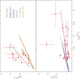
Figure 7: Same as Fig. 5 but comparing our temperature estimates (red points) and temperature relations (red lines represented by Eqs. 3 and 4) with relations obtained from SFs. Orange solid line plots the empirical relation (Eq. 8) obtained by Hägele et al. (2006) using direct temperature estimates for a large sample of H ii galaxies, giant extragalactic H ii regions, Galactic H ii regions, and H ii regions from the MCs. Black solid lines represent the empirical relations (Eqs. 9 and 10) based on direct estimates of disk H ii regions by Rogers et al. (2021). Blue dashed and solid lines, shown only in bottom panel, represent empirical relations for $P\><\>0.5$ and for $P\>>\>0.5$, respectively, based on data compiled from literature by Arellano-Córdova & Rodríguez (2020). P is defined as $([\text{O\,{iii}}]\lambda 4959+\lambda 5007)/[\text{O\,{ii}}]\lambda 3727+[\text{O\,{iii}}]\lambda 4959+\lambda 5007$. Green and pink lines represent the theoretical relations derived by Garnett (1992, Eq.13) and Pérez-Montero & Contini (2009, Eq.14), respectively.

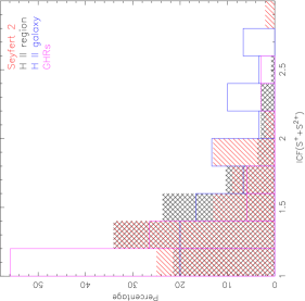
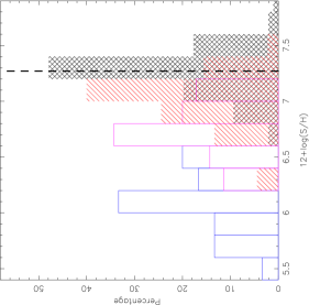
Figure 8: Left panel: distributions for the sulphur ICF (see Sect. 3.2.2). Red distribution is derived from our Sy 2 sample by using Eq. 7 (values listed in Table 7). Black distribution is derived by using values from disk H ii region estimates (i.e. results from CHAOS project) assuming Eq. 7 for $\rm(O^{+}/O)\>\ga\>0.6$ and the theoretical ICF from Thuan et al. (1995) when $\rm(O^{+}/O)\>\la\>0.6$. Blue distribution corresponds to H ii galaxies values from Hägele et al. (2006, 2008); Hägele et al. (2011, 2012) and pink distribution corresponds to GHRs from Hägele et al. (2006), and for both kind of objects the approach proposed by Barker (1980) was used. Right panel: distributions for the sulphur abundance. Dashed line represents the sulphur solar abundance $\rm 12+\log(S/H)_{\odot}=7.27$ derived by Grevesse & Sauval (1998). The color code is the same as in left panel.

4.2 Sulphur abundances

According to the inside-out scheme, galaxies begin to form stars in their inner regions before the outer ones (e.g. Samland et al. 1997; Portinari & Chiosi 1999; Boissier & Prantzos 2000; Sommer-Larsen et al. 2003; Mollá & Díaz 2005; Nelson et al. 2012, 2016; Vincenzo & Kobayashi 2018) producing radial metallicity gradients with negative slopes (i.e. the metalicity decreases with the increase of the galactocentric distance, e.g. Pilyugin et al. 2004). Thus, due to the location of AGNs in galactic disks, they are expected to have high abundance of heavy elements; in other words, AGNs with low abundances are barely found in the local universe (e.g. Groves et al. 2006; Izotov & Thuan 2008; Izotov et al. 2010; Kawasaki et al. 2017; Dors et al. 2020a). However, AGNs seem to have a more complex cosmic chemical evolution than SFs. For instance, Matteucci & Padovani (1993), by means of self-consistent models of galaxy evolution, showed that AGNs in galaxies around the lifetime of $10^{9}$ years ($z\sim 5$) reach an abundance of elements divided into two classes: ($i$) elements with 2-3 times the solar abundance (C, Ne, O and Mg) and ($ii$) the ones with abundances ranging from 5 to 10 times the solar abundance (N, Ni and Fe). Conversely, low abundance or metallicity have been derived at high redshift from SFs (see Curti et al. 2022 and references therein). Despite the fact that Matteucci & Padovani (1993) did not consider sulphur (an $\alpha$-element), its abundance would increase similarly to the oxygen abundance, i.e. the expectation will be a constant S/O abundance ratio.

Optical surveys, such as SDSS, have made plenty of AGNs spectroscopic data available, which make the determinations of quantitative sulphur abundance possible in this class of objects. In this sense, we present a detailed analysis of sulphur abundance from our Sy 2 sample and a comparison with some previous results obtained from SFs. In view of that, we consider the following SF estimates which relied on the $T_{\rm e}$-method:

• Hägele et al. (2006): these authors presented calculations for several heavy elements from a sample of H ii galaxies (33 objects) and Giant H ii Regions (34 objects) by using the $T_{\rm e}$-method. In particular, for the sulphur abundance, they assumed the ICF approach proposed by Barker (1980) with the $\alpha$ exponent equal to 2.5. Following the same procedure, Hägele et al. (2008); Hägele et al. (2011, 2012) studied another 11 H ii galaxies and knots belonging to this kind of objects that we include in our control sample.

• CHAOS project: the Chemical Abundances Of Spirals (CHAOS, Berg et al. 2015) combines the power of the Large Binocular Telescope (LBT) with the broad spectral range and sensitivity of the Multi Object Double Spectrograph (MODS) to derived abundances, which relied on the $T_{\rm e}$-method, for a large sample of H ii regions in spiral galaxies. Taking these valuable data into account, we consider abundance estimates for 135 disk H ii regions located in NGC 5457, NGC 3184 and NGC 2403 by Croxall et al. (2016), Berg et al. (2020) and Rogers et al. (2021), respectively. These authors adopted the sulphur ICF given by Eq. 7 for $\rm(O^{+}/O)\>\ga\>0.6$ and the theoretical ICF from Thuan et al. (1995) when $\rm(O^{+}/O)\>\la\>0.6$.

Along this section, we have used the SF abundance estimates from the above authors as benchmark. We emphasize that any selection effect, such as that which may arise as a result of the existence of auroral lines in spectra, will be present in both our AGN sample and the SF sample taken from the literature.

Our sulphur ICFs for the Seyfert galaxies (listed in Table 7) indicate values between $\sim 1.1$ and $\sim 3.0$, with an averaged value of $1.44$, i.e. about $45\%$ of the sulphur is in higher ionization stages than $\rm S^{2+}$. We found an ICF value higher than 2.0 for only two objects: 2.02 and 2.94 for Mrk 573 and NGC 7674, respectively. Interestingly, for the most extreme ICF value, i.e. for NGC 7674, Kharb et al. (2017), by using radio long baseline interferometry, hinted that this object hosts a Binary Supermassive Black Hole (for a different conclusion see Breiding et al. 2022). Moreover, additional evidence that this object has a hard ionizing spectra is the presence of emission lines of high ionization ions [Ne v]$\lambda 3346,\lambda 3426$, as observed by Kraemer et al. (1994). In any case, even if this object is ruled out from the average ICF calculations, a similar value ($1.40$) is obtained. In order to compare our sulphur ICF values with those from SFs, we consider the ICFs derived by Hägele et al. (2006) and from the CHAOS project. In the left panel of Fig. 8, the distribution of sulphur ICFs for Sy 2s and SFs are shown, where it can be seen that a good agreement exist among them, even though the GHRs present a distribution peak at lower values. It is worth to be noted that most of the objects ($\sim 90\%$) belonging to the distinct object classes present sulphur ICFs lower than $\sim 2$. The range and average of the ICFs for our sample of Sy 2, H ii galaxies, GHRs and disk H ii regions are presented in Table 4 showing that the different samples have similar ICF values. Therefore, despite the fact that Sy 2s have a harder ionizing source than SFs, these two distinct object classes have similar sulphur ionic fractions.

Table 4: Range and average sulphur ICF, S/H, O/H, and S/O abundance values for our sample of Sy 2s, disk H ii regions, H ii galaxies, and Giant H ii regions.

	ICF($\rm S^{+}+S^{2+}$)			12+log(S/H)			12+log(O/H)			log(S/O)		Ref.
Object type	Range	Average		Range	Average		Range	Average		Range	Average
Sy 2	1.1 - 3.0	$1.44$		6.2 - 7.5	$6.98\pm 0.25$		8.0 - 9.1	$8.71\pm 0.24$		$-2.4$ - $-1.3$	$-1.64\pm 0.20$	1
H ii region	1.1 - 2.5	$1.43$		6.2 - 7.9	$7.11\pm 0.28$		7.8 - 8.9	$8.47\pm 0.19$		$-1.7$ - $-0.9$	$-1.35\pm 0.15$	2
H ii galaxy	1.0 - 2.8	$1.66$		5.5 - 6.6	$6.10\pm 0.27$		7.0 - 8.2	$7.79\pm 0.30$		$-2.0$ - $-1.4$	$-1.67\pm 0.15$	3,4
GHR	1.0 - 2.5	$1.26$		6.2 - 7.2	$6.73\pm 0.24$		7.6 - 8.6	$8.12\pm 0.23$		$-1.9$ - $-0.7$	$-1.38\pm 0.30$	4

(1) This work. (2) Croxall et al. (2016), Berg et al. (2020) and Rogers et al. (2021). (3) Hägele et al. (2008); Hägele et al. (2011, 2012). (4) Hägele et al. (2006).

Concerning the total sulphur abundance, in the right panel of Fig. 8, we present the S/H abundance distribution for our sample of Sy 2 nuclei, H ii galaxies and GHRs from Hägele et al. (2006, 2008); Hägele et al. (2011, 2012) and for disk H ii regions from the CHAOS project. Also in this plot, the sulphur solar abundance $\rm 12+\log(S/H)_{\odot}=7.27$ derived by Grevesse & Sauval (1998) is represented by the dashed line. We note that the Sy 2s present an intermediate S/H distribution between that of GHRs and the disk H ii regions, while H ii galaxies tend to present lower sulphur abundances. In Table 4 the range and S/H average values for our AGN sample and for the SF benchmark sample are listed. The Sy 2s present S/H values in the range of $6.2\><\>12+\log(\rm S/H)\><\>7.5$ and considering the sulphur solar value as 12+$\log(\rm S/H)_{\odot}=7.26$ (Grevesse & Sauval, 1998), represents $0.1\><\>(\rm S/S_{\odot})\><\>1.8$, where most of the objects (40/45) have subsolar sulphur abundance. This result can be biased due to the fact that we selected only objects which have the [S iii]$\lambda 9069$ and auroral line [O iii]$\lambda 4363$ measured, resulting (see Table 4) only in Sy 2s with O/H values in the range $8.0\>\la\>12+\log(\rm O/H)\>\la\>9.1$ or $0.2\>\la\>(Z/\rm Z_{\odot})\>\la\>2.6$, adopting the solar oxygen value of $12+\log(\rm O/H)_{\odot}=8.69$ (Allende Prieto et al., 2001). Dors et al. (2020a), who considered a sample of 463 confirmed Seyfert 2 AGNs ($z\>\la\>0.4$) and used distinct methods which did not necessarily required auroral lines, found values in the range $7.1\>\la\>12+\log(\rm O/H)\>\la\>9.2$ or $0.02\>\la\>(Z/\rm Z_{\odot})\>\la\>3.2$. Therefore, lower and higher S/H abundances would be probably derived in the sample if the data by Dors et al. (2020a) could be taken into account. In any case, the abundance estimates from the CHAOS project comprises inner disk H ii regions, therefore, it is expected that these objects and Sy 2 nuclei would have similar S/H abundances, when a large sample of objects is considered. Interestingly, the maximum S/H value ($\sim 7.9$ dex) is derived for disk H ii regions while sulphur abundances in Sy 2s reach up to $\sim 7.5$ dex. This result points to a distinct chemical enrichment of the ISM near the AGNs in comparison to that of the innermost disk H ii regions. We emphasize that a more detailed comparison taking into account SFs and AGNs located in galaxies with similar mass (see do Nascimento et al. 2022) is need to confirm this result.

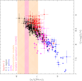
Figure 9: Relation between the total sulphur and oxygen abundances [12+log(S/H) vs. 12+log(O/H)]. Red points represent our Sy 2 nuclei direct estimates. Black points represent estimates from disk H ii regions also obtained through the $T_{\rm e}$-method from the CHAOS project. Pink points represent GHRs estimated from Hägele et al. (2006) and blue ones those estimates for H ii galaxies from Hägele et al. (2006, 2008); Hägele et al. (2011, 2012). The orange hatched area represents the range of S/H values inferred through photoionization models for a sample of 177 Seyfert galaxies by Storchi-Bergmann & Pastoriza (1990). The magenta hatched area represents the range of S/H values obtained from the extrapolation of radial abundance gradients to central parts of four (NGC 0628, NGC 5194, NGC 5457, NGC 3184) spiral galaxies by Berg et al. (2020).

In Fig. 9, we show a plot of the S/H versus O/H abundances for our Sy 2 sample and for the SF benchmark. Also in this figure, the range of the S/H values derived from the photoionization models by Storchi-Bergmann & Pastoriza (1990) and considering a larger sample of AGNs than our data, is indicated. Berg et al. (2020) summarized the radial sulphur gradients (and the gradients for other elements) in four spiral galaxies from the CHAOS project, which are represented by

$$12+\log(\mathrm{S/H})=grad(\mathrm{S})\times R+Y_{0}(\mathrm{S}),$$ (15)

where $grad(\rm S)$ is the value of the slope of the sulphur gradient, $R$ is the radial galactic distance and $Y_{0}(\rm S)$ is the extrapolated value of S/H gradient to the galactic center $R=0$. The range of $Y_{0}(\rm S)$ derived by Berg et al. (2020) is also represented in Fig. 9. We note that, for a given O/H value, in general Sy 2s present lower S/H values than the majority of disk H ii regions and than those from extrapolated gradients. Again, this discrepancy can be due to the distinct chemical evolution of AGNs and SFs or even due to the small AGN sample (the sample contains only 45 objects). H ii galaxies and GHRs present lower S/H and O/H abundances in comparison with the Sy 2s, which indicate that the former objects are less chemically evolved than the latter. Finally, the model results by Storchi-Bergmann & Pastoriza (1990) predicted, on average, higher ($\sim 0.3$ dex) S/H values than those derived by using the $T_{\rm e}$-method for Sy 2s. This discrepancy can be partly due to the known problem of photoionization models overestimating abundances in comparison to the $T_{\rm e}$-method. In fact, Dors et al. (2020b) showed that direct temperature estimates of $T_{\rm e}(\rm O^{2+})$ are higher (up to $11\>000$ K) than those predicted by photoionization models, which translates into an overestimate of the O/H abundance of up to $\sim 1$ dex (with an average value of $\sim 0.2$ dex) by the photoionization models. In order to ascertain if the temperature problem also exists in the sulphur temperatures, in Fig. 10, we compare our direct temperature estimates (shown in Fig. 4) with temperature predictions by the photoionization models built with the Cloudy code by Carvalho et al. (2020) taking into account a wide range of NLR nebular parameters:

• Metallicity: ($Z/\rm Z_{\odot})=3.0,2.0,1.0,0.75,0.5$, and $0.2$.

• Electron density: $N_{\rm e}\>\rm(cm^{-3})=3000,1500,500,100$.

• Ionization parameter ($U$): $\log U$ ranging from $-1.5$ to $-3.5$, with step of 0.5 dex.

• Spectra Energy Distribution (SED): the SED is parametrized by the continuum between 2 keV and 2500Å (Tananbaum et al., 1979) and it is described by a power law with a spectral index $\alpha_{ox}$=$-$0.8, $-$1.1 and $-1.4$.

In Fig. 10, it can be seen that similar to oxygen temperatures (see Dors et al. 2020b) direct temperature estimates for $\rm S^{+}$ and $\rm S^{2+}$ are higher than those predicted by AGN photoioinization models. Thus, this result explains the discrepancy between the sulphur abundance inferred by the photoionization models built by Storchi-Bergmann & Pastoriza (1990) and those calculated from our sample by using the $T_{\rm e}$-method.

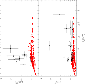
Figure 10: Temperatures (in units of $10^{4}$ K) for the $\rm S^{+}$ (bottom panel) and $\rm S^{2+}$ (upper panel) versus the temperature for $\rm O^{2+}$. Black points are Sy 2 direct estimations which relied on auroral lines (see Sect. 4.1). Red points are temperature predictions by AGN photoionization models built with the Cloudy code by Carvalho et al. (2020).

Finally, in Fig. 11, we show a plot of log(S/O) versus 12+log(O/H), which compares our direct abundance estimates with the SF benchmark. Considering the estimates of all objects (AGN+SF), we provide the following relation

$$\rm\log(S/O)=+0.06(\pm 0.03)\times[12+\log(O/H)]-1.94(\pm 0.33),$$ (16)

with the Pearson coefficient parameters ($R=0.09\pm 0.07$ and p-value = 0.24), i.e. there is no correlation between the estimations. Thus, our estimates combined with those from a large sample of SFs suggest that S/O is constant over a wide range of O/H, as found by recent results from the CHAOS project (see Rogers et al. 2021 and references therein). However, in Fig. 11, it can be seen that there is a clear trend of S/O values of Sy 2 decreasing with O/H in the high metallicity regime. The same behaviour was found from H ii regions, for instance, by Dors et al. (2016) and Díaz & Zamora (2022).

It is worth to mention that emission lines of AGNs, such as [S iii]$\lambda 9069,\lambda 9532$ and auroral lines (mainly [N ii]$\lambda 5755$ and [S iii]$\lambda 6312$) are either measured with low S/N ($\sim 2$) or unavailable in the literature (e.g., see Koski 1978; Dopita et al. 2015). This implies that chemical abundance studies of AGNs are difficult to be carried out and, even when it is possible to determine the abundance directly, higher (a factor of $\sim 2$, see Fig 9) abundance errors in comparison with those of SFs are derived. The next generation of telescopes, such as the Giant Magellan, European Extremely Large, and Thirty Meter Telescopes, will provide higher S/N measurements of weak AGN emission lines and will allow a breakthrough in our understanding of the chemical abundance in AGNs and objects with very high metallicity.

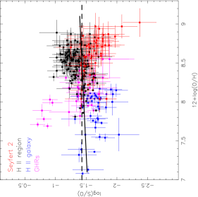
Figure 11: Relation between log(S/O) and 12+log(O/H). Red points represent our Sy 2 nuclei direct estimates. Pink points represent direct estimates for GHRs from Hägele et al. (2006). Black points represent estimates from disk H ii regions obtained also through $T_{\rm e}$-method by Berg et al. (2020). Blue points represent direct estimates for H ii galaxies by Hägele et al. (2006, 2008); Hägele et al. (2011, 2012). Dashed line represents the solar value of $\rm\log(S/O)_{\odot}=-1.43$. Solid line represents the linear regression considering all the estimates given by Eq. 16.

5 Conclusions

We have used observations of the intensities of narrow emission lines in the spectral interval $3000\><\lambda($Å$)\><\>9100$ of sample of 45 nearby ($z\>\la\>0.08$) Seyfert 2 nuclei taken from SDSS DR17 and other compilations from the literature to perform direct estimations of electron temperatures through the $T_{\rm e}$-method and estimates of sulphur and oxygen abundances relative to hydrogen. These estimates were compared with those from local star-forming regions, i.e. disk H ii regions, H ii galaxies and Giant H ii Regions, whose abundance estimates were compiled from the literature. Regarding the electron temperatures, we found that Seyfert 2 and star-forming regions have similar temperature in the gas regions where most $\rm S\rm^{+}$ is located. However, this result is not derived for the zones where most $\rm S\rm^{2+}$ is located: $\rm S^{2+}$ electron temperatures are higher ($\sim 10\>000$ K) from Seyfert 2 than from star-forming regions. We interpret this result as, probably, due to the known feature of SEDs of AGNs are harder than that of SFs, producing a hotter gas in the innermost narrow line region of AGNs. For our sample of Seyfert 2, we derived total sulphur abundances in the range of $6.2\>\la 12+\log(\rm S/H)\>\la\>7.5$ or $0.1\>\la\>(\rm S/S_{\odot})\>\la\>1.8$. The Seyfert 2 sulphur abundances are lower by a factor of $\sim 0.4$ dex than those derived for SFs with similar metallicities. This discrepancy can be interpreted as due to a distinct chemical enrichment of the ISM near the AGNs in comparison to that of the SFs. The relation between S/O and O/H abundance ratios derived from our Seyfert 2 nuclei sample presents an abrupt ($\sim 0.5$ dex) decrease with the increase of O/H for the high metallicity regime [$\rm 12+\log(O/H)\>\ga 8.7)$], which is not derived from star-forming regions. However, when our Sy 2 estimates are combined with those from a large sample of star-forming regions, we did not find any dependence between S/O and O/H, supporting the idea that sulphur and oxygen are produced by stars with similar mass range and that the Initial Mass Function is universal.

Data Availability

The data underlying this article will be shared on reasonable request to the corresponding author.

Appendix A Tables

Table 5: Emission-line intensities of Seyfert 2s relative to H$\beta$=1.00 taken from SDSS DR17 and compiled from the literature. For Mrk 3 the sum [S ii]$\lambda$6717+$6731$ (in relation to H$\beta$) is listed. Last column lists the references for the optical and near infrared lines, except for Mrk 3 and ESO 138 G1 which the line set was taken from only one work.

Object	[O ii]	[O iii]	[O iii]	[N ii]	[S iii]	$\rm H\alpha$	[N ii]	[S ii]	[S ii]	[S iii]	Ref.
	$\lambda$3727	$\lambda$4363	$\lambda$5007	$\lambda$5755	$\lambda$6312	$\lambda$6563	$\lambda$6584	$\lambda$6716	$\lambda$6731	$\lambda$9069+$\lambda$9532
Mrk 573	$2.13\pm 0.05$	$0.14\pm 0.011$	$10.26\pm 0.05$		—	$2.86\pm 0.05$	$2.34\pm 0.04$	$0.79\pm 0.01$	$0.73\pm 0.02$	2.58	1, 12(a)
NGC 5728	$2.32\pm 0.03$	$0.11\pm 0.016$	$9.10\pm 0.11$		—	$2.86\pm 0.13$	$2.86\pm 0.13$	$0.97\pm 0.06$	$0.66\pm 0.03$	1.92	1, 12(a)
ESO 428-G14	2.22	0.24	11.2		—	2.90	3.13	0.83	0.88	1.87	2, 12(a)
NGC 4388	2.73	0.16	10.55		—	2.84	1.50	0.72	0.62	1.10	3, 13(a)
Mrk 78	4.96	0.14	11.94		—	2.46	2.46	0.68	0.61	0.89	4, 14(a)
NGC 7674	1.29	0.12	12.55		—	3.70	3.68	0.54	0.64	3.15	5, 12(a)
NGC 2110	4.38	0.17	4.76		—	2.66	3.76	1.52	1.42	1.91	6, 12(a)
NGC 7682	2.85	0.16	9.34		—	3.10	3.03	1.09	1.17	1.95	7, 12(a)
NGC 3227	3.22	0.50	10.73		—	2.86	5.01	1.24	1.26	1.66	8, 12(b)
Mrk 1066	3.34	0.08	3.84		—	2.76	2.42	0.51	0.55	0.75	9, 12(a)
Mrk 3(b,c)	4.84	0.23	11.22		—	2.85	3.21	1.45		2.59	10
ESO 138 G1(c)	$2.35\pm 0.05$	$0.34\pm 0.02$	$8.71\pm 0.25$		—	$3.01\pm 0.10$	$0.68\pm 0.03$	$0.47\pm 0.03$	$0.48\pm 0.03$	0.69	11
55978-0990	$6.76\pm 0.43$	$0.14\pm 0.06$	$10.70\pm 0.73$		—	$2.86\pm 0.31$	$3.30\pm 0.36$	$1.07\pm 0.18$	$0.87\pm 0.16$	$2.06\pm 0.66$	15
56104-0966	$6.31\pm 0.14$	$0.07\pm 0.02$	$8.51\pm 0.20$		—	$2.86\pm 0.09$	$1.04\pm 0.04$	$0.62\pm 0.03$	$0.56\pm 0.03$	$0.73\pm 0.12$	15
55181-0154	$4.12\pm 0.31$	$0.06\pm 0.03$	$7.82\pm 0.28$		$0.15\pm 0.04$	$2.86\pm 0.21$	$2.05\pm 0.15$	$0.60\pm 0.06$	$0.61\pm 0.06$	$2.02\pm 0.42$	15
56088-0473	$2.07\pm 0.01$	$0.06\pm 0.01$	$7.70\pm 0.04$		$0.01\pm 0.01$	$2.86\pm 0.01$	$0.15\pm 0.01$	$0.12\pm 0.01$	$0.11\pm 0.01$	$0.63\pm 0.02$	15
56034-0154	$3.02\pm 0.32$	$0.14\pm 0.01$	$11.88\pm 0.23$		$0.05\pm 0.03$	$2.86\pm 0.07$	$2.13\pm 0.05$	$0.88\pm 0.03$	$0.81\pm 0.03$	$2.10\pm 0.14$	15
56067-0382	$5.51\pm 1.33$	$0.21\pm 0.10$	$8.70\pm 0.83$	$0.192\pm 0.165$	—	$2.86\pm 0.52$	$2.36\pm 0.44$	$0.86\pm 0.22$	$0.81\pm 0.22$	$1.19\pm 0.89$	15
56240-0340	$8.32\pm 0.52$	$0.16\pm 0.06$	$7.24\pm 0.56$		—	$2.86\pm 0.28$	$2.60\pm 0.26$	$1.10\pm 0.21$	$0.86\pm 0.20$	$3.04\pm 0.94$	15
55539-0167	$2.79\pm 0.20$	$0.05\pm 0.02$	$4.11\pm 0.08$	$0.078\pm 0.047$	—	$2.86\pm 0.08$	$1.91\pm 0.05$	$0.61\pm 0.03$	$0.54\pm 0.03$	$1.08\pm 0.14$	15
56626-0636	$3.82\pm 0.09$	$0.06\pm 0.01$	$6.12\pm 0.10$		$0.10\pm 0.02$	$2.86\pm 0.07$	$2.23\pm 0.05$	$1.06\pm 0.03$	$0.98\pm 0.03$	$1.22\pm 0.10$	15
56074-0045	$4.23\pm 0.32$	$0.03\pm 0.01$	$2.69\pm 0.04$		—	$2.86\pm 0.07$	$1.52\pm 0.04$	$0.77\pm 0.02$	$0.58\pm 0.02$	$0.91\pm 0.11$	15
55212-0380	$3.52\pm 1.13$	$0.10\pm 0.03$	$12.54\pm 0.51$		—	$2.86\pm 0.15$	$2.94\pm 0.15$	$0.85\pm 0.06$	$0.84\pm 0.06$	$2.41\pm 0.30$	15
56399-0302	$5.01\pm 0.37$	$0.08\pm 0.04$	$3.07\pm 0.19$		—	$2.86\pm 0.23$	$2.16\pm 0.19$	$1.58\pm 0.16$	$1.14\pm 0.14$	$1.33\pm 0.63$	15
56001-0293	$5.05\pm 0.20$	$0.07\pm 0.01$	$7.63\pm 0.20$	$0.047\pm 0.037$	—	$2.86\pm 0.13$	$1.74\pm 0.08$	$0.85\pm 0.05$	$0.61\pm 0.04$	$1.54\pm 0.21$	15
55651-0052	$3.28\pm 0.76$	$0.02\pm 0.01$	$3.54\pm 0.04$		$0.05\pm 0.01$	$2.86\pm 0.06$	$2.06\pm 0.04$	$0.72\pm 0.02$	$0.68\pm 0.02$	$0.94\pm 0.08$	15
56566-0794	$6.58\pm 0.61$	$0.05\pm 0.02$	$4.74\pm 0.12$	$0.017\pm 0.016$	$0.08\pm 0.03$	$2.86\pm 0.10$	$2.16\pm 0.08$	$1.26\pm 0.06$	$1.07\pm 0.05$	$1.22\pm 0.16$	15
56748-0336	$4.97\pm 0.51$	$0.08\pm 0.05$	$7.11\pm 0.41$		—	$2.86\pm 0.24$	$3.23\pm 0.27$	$0.99\pm 0.12$	$0.89\pm 0.12$	$1.85\pm 0.50$	15
56206-0454	$7.35\pm 0.27$	$0.09\pm 0.02$	$6.67\pm 0.19$		$0.05\pm 0.03$	$2.86\pm 0.11$	$1.21\pm 0.06$	$1.12\pm 0.05$	$0.91\pm 0.05$	$1.08\pm 0.19$	15
55860-0112	$5.74\pm 1.44$	$0.11\pm 0.07$	$7.82\pm 0.66$		$0.15\pm 0.12$	$2.86\pm 0.33$	$5.38\pm 0.61$	$1.80\pm 0.23$	$1.77\pm 0.23$	$1.78\pm 0.46$	15
56453-0144	$3.19\pm 0.37$	$0.06\pm 0.02$	$6.42\pm 0.18$		—	$2.86\pm 0.10$	$2.64\pm 0.10$	$0.89\pm 0.06$	$0.78\pm 0.06$	$2.20\pm 0.31$	15
55710-0116	$2.72\pm 1.05$	$0.07\pm 0.02$	$7.54\pm 0.24$		$0.06\pm 0.04$	$2.86\pm 0.12$	$4.47\pm 0.18$	$1.04\pm 0.06$	$1.13\pm 0.07$	$2.58\pm 0.21$	15
56209-0390	$6.99\pm 0.77$	$0.07\pm 0.06$	$8.57\pm 0.97$		—	$2.86\pm 0.58$	$2.75\pm 0.55$	$0.39\pm 0.15$	$0.22\pm 0.14$	$0.52\pm 0.65$	15
56298-0302	$10.16\pm 1.84$	$0.09\pm 0.07$	$5.39\pm 0.46$		—	$2.86\pm 0.42$	$3.29\pm 0.49$	$1.59\pm 0.27$	$1.40\pm 0.24$	$7.00\pm 2.26$	15
56366-0928	$4.81\pm 0.41$	$0.12\pm 0.05$	$5.70\pm 0.40$		$0.21\pm 0.08$	$2.86\pm 0.28$	$2.51\pm 0.25$	$0.96\pm 0.12$	$0.96\pm 0.12$	$2.31\pm 0.56$	15
55742-0383	$2.74\pm 0.55$	$0.05\pm 0.01$	$4.99\pm 0.10$	$0.049\pm 0.038$	—	$2.86\pm 0.08$	$2.06\pm 0.06$	$0.63\pm 0.03$	$0.56\pm 0.03$	$1.01\pm 0.14$	15
55302-0655	$4.90\pm 0.18$	$0.05\pm 0.02$	$2.06\pm 0.05$	$0.035\pm 0.019$	—	$2.86\pm 0.08$	$1.67\pm 0.06$	$1.24\pm 0.04$	$1.00\pm 0.04$	$0.94\pm 0.14$	15
56328-0550	$6.45\pm 0.26$	$0.06\pm 0.02$	$4.90\pm 0.15$		$0.06\pm 0.04$	$2.86\pm 0.13$	$3.35\pm 0.16$	$1.10\pm 0.06$	$0.86\pm 0.06$	$1.57\pm 0.25$	15
55646-0770	$8.48\pm 2.32$	$0.14\pm 0.05$	$7.32\pm 1.31$		—	$2.86\pm 0.95$	$3.74\pm 1.23$	$1.50\pm 0.56$	$1.39\pm 0.52$	$1.82\pm 1.49$	15
55617-0758	$8.05\pm 0.33$	$0.05\pm 0.04$	$3.84\pm 0.20$		$0.11\pm 0.06$	$2.86\pm 0.27$	$2.26\pm 0.22$	$1.24\pm 0.14$	$1.38\pm 0.15$	$1.33\pm 0.40$	15
56003-0218	$3.35\pm 1.00$	$0.07\pm 0.04$	$4.70\pm 0.29$		$0.10\pm 0.07$	$2.86\pm 0.22$	$1.68\pm 0.15$	$0.56\pm 0.09$	$0.58\pm 0.09$	$2.06\pm 0.45$	15
55629-0364	$9.11\pm 0.64$	$0.11\pm 0.07$	$7.08\pm 0.52$		—	$2.86\pm 0.41$	$3.91\pm 0.57$	$1.44\pm 0.24$	$1.32\pm 0.23$	$1.64\pm 0.80$	15
56568-0076	$5.12\pm 0.59$	$0.03\pm 0.01$	$3.16\pm 0.05$	$0.031\pm 0.021$	—	$2.86\pm 0.09$	$2.98\pm 0.10$	$0.71\pm 0.03$	$0.69\pm 0.03$	$0.66\pm 0.09$	15
55836-0160	$3.57\pm 0.33$	$0.04\pm 0.02$	$3.70\pm 0.11$		—	$2.86\pm 0.14$	$2.24\pm 0.11$	$0.67\pm 0.05$	$0.59\pm 0.05$	$1.71\pm 0.32$	15
55505-0654	$3.05\pm 0.19$	$0.04\pm 0.02$	$7.95\pm 0.28$		$0.05\pm 0.03$	$2.86\pm 0.17$	$2.70\pm 0.16$	$0.65\pm 0.05$	$0.58\pm 0.05$	$2.10\pm 0.35$	15

References— (1) Dopita et al. (2015), (2) Bergvall et al. (1986), (3) Phillips et al. (1983), (4) Koski (1978), (5) Kraemer et al. (1994), (6) Shuder (1980), (7) Thomas et al. (2017), (8) Cohen (1983), (6) Goodrich & Osterbrock (1983), (10) Malkan & Oke (1983), (11) Alloin et al. (1992). (12) Riffel et al. (2006), (13) Rodríguez-Ardila et al. (2011), (14) Ramos Almeida et al. (2006), (15) BOSS/SDSS sample, (a) Reference which the [S iii]$\lambda 9069$ emission line fluxes was compiled. (b) Emission-line intensities corrected by reddening in the present work. (c) Object which the [S iii]$\lambda 9069$ was measured with the others.

Table 6: Electron density and electron temperature values assumed in the ionic abundance calculations. $T_{\rm e}(\rm O^{2+})$ was calculated through the observational $RO3$ line ratio, whose line intensities are listed in Table 5, and by using the PyNeb code (Luridiana et al., 2015). $T_{\rm e}(\rm N^{+})$ and $T_{\rm e}(\rm S^{2+})$ were calculated either from $RN2$ and $RS3$ line ratios (when these line ratios were measured), respectively, or from Eq. 3 and 4 (when auroral lines were not measured, see Table 5).

Object	$T_{\rm e}(\rm O^{2+})$ K	$T_{\rm e}(\rm S^{2+})$ K	$T_{\rm e}(\rm N^{+})$ K	$N_{\rm e}(\rm cm^{-3}$)
Mrk 573	$12888\pm 425$	$21341\pm 7881$	$11673\pm 1899$	$559\pm 102$
NGC 5728	$12301\pm 725$	$20030\pm 7929$	$11373\pm 1923$	$674\pm 167$
ESO 428-G14	$15651\pm 1197$	$27501\pm 8055$	$13082\pm 1983$	$1059\pm 466$
NGC 4388	$13446\pm 1254$	$22585\pm 8074$	$11958\pm 1992$	393:
Mrk 78	$12162\pm 1139$	$19721\pm 8036$	$11303\pm 1974$	475:
NGC 7674	$11296\pm 1126$	$17790\pm 8032$	$10861\pm 1972$	$1396\pm 620$
NGC 2110	$20761\pm 3395$	$38896\pm 9338$	$15688\pm 2561$	$691\pm 300$
NGC 7682	$14146\pm 1412$	$24146\pm 8131$	$12315\pm 2020$	$1067\pm 495$
NGC 3227	$25028\pm 2500$	$48412\pm 17000$	$17864\pm 5800$	$1067\pm 485$
Mrk 1066	$15446\pm 3553$	$27045\pm 9466$	$12978\pm 2616$	1122:
Mrk 3	$15335\pm 1185$	$26796\pm 8051$	$12921\pm 1981$	500:
ESO 138 G1	$21996\pm 1318$	$41650\pm 8097$	$16318\pm 2003$	$1039\pm 452$
55978-0990	$12685\pm 2490$	$20888\pm 8684$	$11570\pm 2274$	266:
56104-0966	$10754\pm 1095$	$16582\pm 8023$	$10585\pm 1968$	$471\pm 210$
55181-0154	$10508\pm 1855$	$24392\pm 9679$	$10459\pm 2111$	$778\pm 384$
56088-0473	$10566\pm 301$	$9244\pm 1351$	$10488\pm 1893$	$502\pm 186$
56034-0154	$12184\pm 409$	$11052\pm 2481$	$11314\pm 1898$	$537\pm 167$
56067-0382	$16612\pm 5030$	$29644\pm 10845$	$31422\pm 9900$	666:
56240-0340	$15912\pm 3588$	$28083\pm 9495$	$13215\pm 2628$	200:
55539-0167	$12334\pm 1976$	$20105\pm 8387$	$16670\pm 5500$	$445\pm 218$
56626-0636	$11409\pm 726$	$27152\pm 5997$	$10919\pm 1923$	$537\pm 137$
56074-0045	$11954\pm 1531$	$19258\pm 8179$	$11197\pm 2042$	$127\pm 58$
55212-0380	$10644\pm 1185$	$16335\pm 8051$	$10528\pm 1981$	$699\pm 315$
56399-0302	$17311\pm 5347$	$31203\pm 11175$	$13929\pm 3316$	50:
56001-0293	$11159\pm 640$	$17484\pm 7913$	$13152\pm 4500$	55:
55651-0052	$9576\pm 733$	$18122\pm 2797$	$9984\pm 1923$	$555\pm 130$
56566-0794	$11713\pm 1806$	$21676\pm 7539$	$10771\pm 3800$	$347\pm 162$
56748-0336	$11981\pm 3128$	$19319\pm 9129$	$11211\pm 2471$	477:
56206-0454	$12842\pm 1266$	$16315\pm 7012$	$11649\pm 1994$	$266\pm 130$
55860-0112	$13038\pm 3931$	$27975\pm 12880$	$11749\pm 2753$	$735\pm 360$
56453-0144	$11224\pm 1400$	$17630\pm 8127$	$10824\pm 2017$	$410\pm 202$
55710-0116	$11189\pm 1218$	$10917\pm 2756$	$10806\pm 1986$	$1021\pm 381$
56209-0390	$10735\pm 3862$	$16538\pm 8150$	$10575\pm 2728$	$198\pm 49$
56298-0302	$14006\pm 5604$	$23833\pm 11451$	$12243\pm 3425$	$451\pm 215$
56366-0928	$15523\pm 3682$	$30648\pm 9727$	$13017\pm 2662$	$839\pm 410$
55742-0383	$11497\pm 889$	$18239\pm 7966$	$12245\pm 3500$	$445\pm 206$
55302-0655	$16672\pm 3674$	$29778\pm 9568$	$11547\pm 3178$	$267\pm 122$
56328-0550	$12373\pm 1714$	$14346\pm 5621$	$11410\pm 2080$	192:
55646-0770	$14856\pm 3805$	$25729\pm 9680$	$12676\pm 2706$	593:
55617-0758	$12640\pm 4540$	$27347\pm 10109$	$11546\pm 2987$	$1168\pm 560$
56003-0218	$13337\pm 3563$	$16884\pm 8330$	$11902\pm 2620$	$913\pm 430$
55629-0364	$13575\pm 4192$	$22872\pm 10028$	$12023\pm 2852$	546:
56568-0076	$11281\pm 1368$	$17756\pm 8115$	$10853\pm 2012$	$666\pm 215$
55836-0160	$11814\pm 2314$	$18946\pm 8576$	$11125\pm 2225$	$427\pm 205$
55505-0654	$9268\pm 1446$	$11052\pm 2955$	$9827\pm 2026$	$422\pm 190$
Note. For some objects we use “:” to indicate that error bars are at least an order
of magnitude larger than the expected density. This is due to the significant
emission-line errors (see Sect 3.1).

Table 7: Ionic and total abundances for Seyfert 2 nuclei derived through the $T_{\rm e}$-method.

Object	$\rm O^{+}/H^{+}$	$\rm O^{2+}/H^{+}$	O/H	$\rm S^{+}/H^{+}$	$\rm S^{2+}/H^{+}$	ICF(S)	S/H	S/O
Mrk 573	$7.95\pm 0.12$	$8.21\pm 0.04$	$8.58\pm 0.13$	$6.46\pm 0.12$	$6.52\pm 0.16$	$2.02$	$7.08\pm 0.18$	$-1.50\pm 0.22$
NGC 5728	$8.03\pm 0.12$	$8.22\pm 0.07$	$8.61\pm 0.14$	$6.52\pm 0.12$	$6.42\pm 0.17$	$1.81$	$7.07\pm 0.18$	$-1.55\pm 0.23$
ESO 428-G14	$7.79\pm 0.10$	$8.03\pm 0.07$	$8.40\pm 0.12$	$6.44\pm 0.10$	$6.24\pm 0.15$	$1.95$	$6.94\pm 0.16$	$-1.46\pm 0.20$
NGC 4388	$8.03\pm 0.12$	$8.17\pm 0.09$	$8.59\pm 0.13$	$6.37\pm 0.12$	$6.12\pm 0.16$	$1.83$	$6.85\pm 0.18$	$-1.74\pm 0.22$
Mrk 78	$8.38\pm 0.13$	$8.35\pm 0.10$	$8.84\pm 0.14$	$6.41\pm 0.13$	$6.10\pm 0.17$	$1.52$	$6.87\pm 0.19$	$-1.97\pm 0.23$
NGC 7674	$7.85\pm 0.13$	$8.47\pm 0.10$	$8.74\pm 0.15$	$6.47\pm 0.13$	$6.71\pm 0.18$	$2.94$	$7.20\pm 0.19$	$-1.54\pm 0.24$
NGC 2110	$7.84\pm 0.10$	$7.39\pm 0.09$	$8.15\pm 0.11$	$6.50\pm 0.10$	$6.30\pm 0.14$	$1.22$	$6.71\pm 0.16$	$-1.43\pm 0.19$
NGC 7682	$7.99\pm 0.12$	$8.06\pm 0.09$	$8.50\pm 0.13$	$6.61\pm 0.11$	$6.33\pm 0.16$	$1.61$	$7.08\pm 0.17$	$-1.42\pm 0.22$
NGC 3227	$7.55\pm 0.14$	$7.59\pm 0.06$	$8.04\pm 0.15$	$6.36\pm 0.15$	$6.28\pm 0.19$	$1.72$	$6.62\pm 0.21$	$-1.42\pm 0.26$
Mrk 1066	$7.98\pm 0.13$	$7.58\pm 0.11$	$8.30\pm 0.14$	$6.24\pm 0.13$	$5.85\pm 0.17$	$1.21$	$6.68\pm 0.19$	$-1.62\pm 0.24$
Mrk 3	$8.16\pm 0.11$	$8.05\pm 0.07$	$8.58\pm 0.12$	$6.62\pm 0.11$	$6.40\pm 0.15$	$1.46$	$7.11\pm 0.17$	$-1.47\pm 0.21$
ESO 138 G1	$7.52\pm 0.08$	$7.60\pm 0.05$	$8.04\pm 0.09$	$6.00\pm 0.08$	$5.78\pm 0.12$	$1.74$	$6.20\pm 0.14$	$-1.83\pm 0.16$
55978-0990	$8.49\pm 0.14$	$8.25\pm 0.09$	$8.86\pm 0.15$	$6.55\pm 0.14$	$6.43\pm 0.18$	$1.35$	$7.09\pm 0.20$	$-1.78\pm 0.25$
56104-0966	$8.60\pm 0.14$	$8.37\pm 0.11$	$8.97\pm 0.15$	$6.44\pm 0.14$	$6.12\pm 0.18$	$1.32$	$6.90\pm 0.20$	$-2.08\pm 0.25$
55181-0154	$8.42\pm 0.15$	$8.36\pm 0.11$	$8.87\pm 0.16$	$6.48\pm 0.15$	$6.34\pm 0.19$	$1.43$	$7.01\pm 0.21$	$-1.86\pm 0.26$
56088-0473	$8.13\pm 0.14$	$8.35\pm 0.04$	$8.73\pm 0.15$	$5.74\pm 0.14$	$6.50\pm 0.18$	$1.89$	$6.86\pm 0.20$	$-1.87\pm 0.25$
56034-0154	$8.16\pm 0.12$	$8.35\pm 0.04$	$8.74\pm 0.14$	$6.53\pm 0.12$	$6.87\pm 0.17$	$1.87$	$7.32\pm 0.18$	$-1.41\pm 0.23$
56067-0382	$7.58\pm 0.16$	$7.86\pm 0.13$	$8.04\pm 0.17$	$6.03\pm 0.15$	$6.01\pm 0.19$	$1.31$	$6.32\pm 0.21$	$-1.72\pm 0.27$
56240-0340	$8.38\pm 0.13$	$7.82\pm 0.10$	$8.66\pm 0.14$	$6.43\pm 0.13$	$6.44\pm 0.17$	$1.18$	$7.03\pm 0.19$	$-1.63\pm 0.23$
55539-0167	$7.58\pm 0.15$	$7.87\pm 0.10$	$8.22\pm 0.16$	$6.03\pm 0.15$	$6.17\pm 0.20$	$1.32$	$6.70\pm 0.22$	$-1.53\pm 0.27$
56626-0636	$8.32\pm 0.13$	$8.14\pm 0.07$	$8.72\pm 0.14$	$6.65\pm 0.13$	$6.06\pm 0.17$	$1.35$	$7.04\pm 0.19$	$-1.68\pm 0.24$
56074-0045	$8.35\pm 0.13$	$7.73\pm 0.09$	$8.62\pm 0.14$	$6.41\pm 0.13$	$6.12\pm 0.17$	$1.15$	$6.88\pm 0.19$	$-1.74\pm 0.24$
55212-0380	$8.34\pm 0.14$	$8.55\pm 0.10$	$8.94\pm 0.15$	$6.62\pm 0.14$	$6.65\pm 0.18$	$1.81$	$7.22\pm 0.20$	$-1.71\pm 0.25$
56399-0302	$8.10\pm 0.14$	$7.37\pm 0.12$	$8.35\pm 0.15$	$6.51\pm 0.14$	$6.47\pm 0.18$	$1.13$	$6.79\pm 0.20$	$-1.56\pm 0.25$
56001-0293	$8.19\pm 0.17$	$8.27\pm 0.07$	$8.71\pm 0.18$	$6.29\pm 0.15$	$6.41\pm 0.19$	$1.38$	$6.95\pm 0.21$	$-1.76\pm 0.28$
55651-0052	$8.41\pm 0.15$	$8.16\pm 0.10$	$8.78\pm 0.16$	$6.58\pm 0.15$	$6.17\pm 0.19$	$1.28$	$7.01\pm 0.21$	$-1.77\pm 0.26$
56566-0794	$8.57\pm 0.13$	$8.00\pm 0.11$	$8.85\pm 0.14$	$7.06\pm 0.16$	$6.18\pm 0.20$	$1.16$	$7.40\pm 0.22$	$-1.45\pm 0.26$
56748-0336	$8.39\pm 0.15$	$8.14\pm 0.12$	$8.76\pm 0.16$	$6.58\pm 0.15$	$6.43\pm 0.19$	$1.32$	$7.10\pm 0.21$	$-1.66\pm 0.26$
56206-0454	$8.51\pm 0.12$	$8.03\pm 0.10$	$8.81\pm 0.14$	$6.56\pm 0.12$	$6.30\pm 0.17$	$1.20$	$7.04\pm 0.18$	$-1.77\pm 0.23$
55860-0112	$8.37\pm 0.15$	$8.08\pm 0.12$	$8.72\pm 0.16$	$6.83\pm 0.15$	$6.21\pm 0.19$	$1.27$	$7.22\pm 0.21$	$-1.51\pm 0.27$
56453-0144	$8.26\pm 0.14$	$8.19\pm 0.09$	$8.70\pm 0.15$	$6.56\pm 0.14$	$6.56\pm 0.18$	$1.47$	$7.15\pm 0.20$	$-1.55\pm 0.25$
55710-0116	$8.18\pm 0.13$	$8.26\pm 0.11$	$8.70\pm 0.15$	$6.72\pm 0.13$	$6.97\pm 0.18$	$1.58$	$7.45\pm 0.20$	$-1.25\pm 0.24$
56209-0390	$8.66\pm 0.17$	$8.38\pm 0.13$	$9.02\pm 0.18$	$6.12\pm 0.14$	$5.97\pm 0.19$	$1.32$	$6.65\pm 0.20$	$-2.37\pm 0.27$
56298-0302	$8.56\pm 0.16$	$7.83\pm 0.13$	$8.81\pm 0.17$	$6.70\pm 0.15$	$6.89\pm 0.19$	$1.10$	$7.40\pm 0.21$	$-1.42\pm 0.27$
56366-0928	$8.13\pm 0.13$	$7.74\pm 0.11$	$8.46\pm 0.14$	$6.48\pm 0.13$	$6.81\pm 0.17$	$1.22$	$6.98\pm 0.19$	$-1.48\pm 0.24$
55742-0383	$7.99\pm 0.16$	$8.04\pm 0.09$	$8.50\pm 0.17$	$6.30\pm 0.15$	$6.20\pm 0.20$	$1.41$	$6.84\pm 0.21$	$-1.65\pm 0.28$
55302-0655	$8.35\pm 0.16$	$7.23\pm 0.11$	$8.56\pm 0.18$	$6.61\pm 0.15$	$5.91\pm 0.20$	$1.09$	$6.98\pm 0.21$	$-1.58\pm 0.28$
56328-0550	$8.50\pm 0.13$	$7.94\pm 0.11$	$8.78\pm 0.14$	$6.56\pm 0.13$	$6.55\pm 0.17$	$1.17$	$7.15\pm 0.19$	$-1.63\pm 0.24$
55646-0770	$8.42\pm 0.13$	$7.90\pm 0.11$	$8.71\pm 0.15$	$6.66\pm 0.14$	$6.26\pm 0.18$	$1.17$	$7.10\pm 0.20$	$-1.62\pm 0.25$
55617-0758	$8.54\pm 0.16$	$7.81\pm 0.12$	$8.79\pm 0.17$	$6.74\pm 0.16$	$6.10\pm 0.21$	$1.09$	$7.12\pm 0.22$	$-1.67\pm 0.28$
56003-0218	$8.11\pm 0.14$	$7.83\pm 0.11$	$8.47\pm 0.15$	$6.34\pm 0.14$	$6.56\pm 0.19$	$1.27$	$7.05\pm 0.20$	$-1.42\pm 0.26$
55629-0364	$8.54\pm 0.15$	$7.99\pm 0.12$	$8.82\pm 0.16$	$6.69\pm 0.15$	$6.28\pm 0.19$	$1.16$	$7.12\pm 0.21$	$-1.70\pm 0.26$
56568-0076	$8.45\pm 0.14$	$7.87\pm 0.10$	$8.73\pm 0.15$	$6.50\pm 0.13$	$6.03\pm 0.18$	$1.13$	$6.92\pm 0.20$	$-1.81\pm 0.25$
55836-0160	$8.26\pm 0.14$	$7.88\pm 0.11$	$8.59\pm 0.15$	$6.41\pm 0.14$	$6.41\pm 0.18$	$1.23$	$7.00\pm 0.20$	$-1.59\pm 0.25$
55505-0654	$8.42\pm 0.15$	$8.56\pm 0.11$	$8.97\pm 0.17$	$6.53\pm 0.16$	$6.87\pm 0.20$	$1.74$	$7.33\pm 0.22$	$-1.65\pm 0.27$

References

- Abazajian et al. (2005) Abazajian K., et al., 2005, AJ, 129, 1755
- Abazajian et al. (2009) Abazajian K. N., et al., 2009, ApJS, 182, 543
- Abdurro’uf et al. (2022) Abdurro’uf et al., 2022, ApJS, 259, 35
- Aihara et al. (2011) Aihara H., et al., 2011, ApJS, 193, 29
- Aldrovandi & Contini (1984) Aldrovandi S. M. V., Contini M., 1984, A&A, 140, 368
- Allende Prieto et al. (2001) Allende Prieto C., Lambert D. L., Asplund M., 2001, ApJ, 556, L63
- Allende Prieto et al. (2004) Allende Prieto C., Barklem P. S., Lambert D. L., Cunha K., 2004, A&A, 420, 183
- Aller & Czyzak (1983) Aller L. H., Czyzak S. J., 1983, ApJS, 51, 211
- Alloin et al. (1992) Alloin D., Bica E., Bonatto C., Prugniel P., 1992, A&A, 266, 117
- Arellano-Córdova & Rodríguez (2020) Arellano-Córdova K. Z., Rodríguez M., 2020, MNRAS, 497, 672
- Arellano-Córdova et al. (2020) Arellano-Córdova K. Z., Esteban C., García-Rojas J., Méndez-Delgado J. E., 2020, MNRAS, 496, 1051
- Arellano-Córdova et al. (2022) Arellano-Córdova K. Z., et al., 2022, ApJ, 935, 74
- Armah et al. (2021) Armah M., et al., 2021, MNRAS, 508, 371
- Armus et al. (2022) Armus L., et al., 2022, arXiv e-prints, p. arXiv:2209.13125
- Barker (1980) Barker T., 1980, ApJ, 240, 99
- Bedregal et al. (2009) Bedregal A. G., Colina L., Alonso-Herrero A., Arribas S., 2009, ApJ, 698, 1852
- Berg et al. (2013) Berg D. A., Skillman E. D., Garnett D. R., Croxall K. V., Marble A. R., Smith J. D., Gordon K., Kennicutt Robert C. J., 2013, ApJ, 775, 128
- Berg et al. (2015) Berg D. A., Skillman E. D., Croxall K. V., Pogge R. W., Moustakas J., Johnson-Groh M., 2015, ApJ, 806, 16
- Berg et al. (2020) Berg D. A., Pogge R. W., Skillman E. D., Croxall K. V., Moustakas J., Rogers N. S. J., Sun J., 2020, ApJ, 893, 96
- Bergvall et al. (1986) Bergvall N., Johansson L., Olofsson K., 1986, A&A, 166, 92
- Bernard-Salas et al. (2008) Bernard-Salas J., Pottasch S. R., Gutenkunst S., Morris P. W., Houck J. R., 2008, ApJ, 672, 274
- Bianchi et al. (2010) Bianchi S., Chiaberge M., Evans D. A., Guainazzi M., Baldi R. D., Matt G., Piconcelli E., 2010, MNRAS, 405, 553
- Binette et al. (2012) Binette L., Matadamas R., Hägele G. F., Nicholls D. C., Magris C. G., Peña-Guerrero M. Á., Morisset C., Rodríguez-González A., 2012, A&A, 547, A29
- Bogdán et al. (2017) Bogdán Á., Kraft R. P., Evans D. A., Andrade-Santos F., Forman W. R., 2017, ApJ, 848, 61
- Boissier & Prantzos (2000) Boissier S., Prantzos N., 2000, MNRAS, 312, 398
- Bonifacio et al. (2001) Bonifacio P., Caffau E., Centurión M., Molaro P., Vladilo G., 2001, MNRAS, 325, 767
- Breiding et al. (2022) Breiding P., Burke-Spolaor S., An T., Bansal K., Mohan P., Taylor G. B., Zhang Y., 2022, ApJ, 933, 143
- Busch et al. (2016) Busch G., et al., 2016, A&A, 587, A138
- Caffau et al. (2005) Caffau E., Bonifacio P., Faraggiana R., François P., Gratton R. G., Barbieri M., 2005, A&A, 441, 533
- Cardaci et al. (2009) Cardaci M. V., Santos-Lleó M., Krongold Y., Hägele G. F., Díaz A. I., Rodríguez-Pascual P., 2009, A&A, 505, 541
- Cardaci et al. (2011) Cardaci M. V., Santos-Lleó M., Hägele G. F., Krongold Y., Díaz A. I., Rodríguez-Pascual P., 2011, A&A, 530, A125
- Cardelli et al. (1989) Cardelli J. A., Clayton G. C., Mathis J. S., 1989, ApJ, 345, 245
- Carvalho et al. (2020) Carvalho S. P., et al., 2020, MNRAS, 492, 5675
- Castro et al. (2017) Castro C. S., Dors O. L., Cardaci M. V., Hägele G. F., 2017, MNRAS, 467, 1507
- Cavichia et al. (2017) Cavichia O., Costa R. D. D., Maciel W. J., Mollá M., 2017, MNRAS, 468, 272
- Centurión et al. (2000) Centurión M., Bonifacio P., Molaro P., Vladilo G., 2000, ApJ, 536, 540
- Cerqueira-Campos et al. (2021) Cerqueira-Campos F. C., Rodríguez-Ardila A., Riffel R., Marinello M., Prieto A., Dahmer-Hahn L. G., 2021, MNRAS, 500, 2666
- Chevallard & Charlot (2016) Chevallard J., Charlot S., 2016, MNRAS, 462, 1415
- Christensen et al. (1997) Christensen T., Petersen L., Gammelgaard P., 1997, A&A, 322, 41
- Cid Fernandes et al. (2005) Cid Fernandes R., Mateus A., Sodré L., Stasińska G., Gomes J. M., 2005, MNRAS, 358, 363
- Cid Fernandes et al. (2010) Cid Fernandes R., Stasińska G., Schlickmann M. S., Mateus A., Vale Asari N., Schoenell W., Sodré L., 2010, MNRAS, 403, 1036
- Cohen (1983) Cohen R. D., 1983, ApJ, 273, 489
- Congiu et al. (2017) Congiu E., et al., 2017, MNRAS, 471, 562
- Costa Silva et al. (2020) Costa Silva A. R., Delgado Mena E., Tsantaki M., 2020, A&A, 634, A136
- Costa et al. (2004) Costa R. D. D., Uchida M. M. M., Maciel W. J., 2004, A&A, 423, 199
- Croxall et al. (2015) Croxall K. V., Pogge R. W., Berg D. A., Skillman E. D., Moustakas J., 2015, ApJ, 808, 42
- Croxall et al. (2016) Croxall K. V., Pogge R. W., Berg D. A., Skillman E. D., Moustakas J., 2016, ApJ, 830, 4
- Curti et al. (2022) Curti M., et al., 2022, MNRAS,
- Danehkar et al. (2022) Danehkar A., Oey M. S., Gray W. J., 2022, ApJ, 937, 68
- Davies et al. (2014) Davies R. L., Rich J. A., Kewley L. J., Dopita M. A., 2014, MNRAS, 439, 3835
- Delgado-Inglada et al. (2014) Delgado-Inglada G., Morisset C., Stasińska G., 2014, MNRAS, 440, 536
- Denicoló et al. (2002) Denicoló G., Terlevich R., Terlevich E., 2002, MNRAS, 330, 69
- Diamond-Stanic & Rieke (2012) Diamond-Stanic A. M., Rieke G. H., 2012, ApJ, 746, 168
- Díaz & Zamora (2022) Díaz Á. I., Zamora S., 2022, MNRAS, 511, 4377
- Díaz et al. (2007) Díaz Á. I., Terlevich E., Castellanos M., Hägele G. F., 2007, MNRAS, 382, 251
- Dopita & Sutherland (1995) Dopita M. A., Sutherland R. S., 1995, ApJ, 455, 468
- Dopita et al. (2005) Dopita M. A., et al., 2005, ApJ, 619, 755
- Dopita et al. (2015) Dopita M. A., et al., 2015, ApJS, 217, 12
- Dors et al. (2008) Dors O. L. J., Storchi-Bergmann T., Riffel R. A., Schimdt A. A., 2008, A&A, 482, 59
- Dors et al. (2014) Dors O. L., Cardaci M. V., Hägele G. F., Krabbe Â. C., 2014, MNRAS, 443, 1291
- Dors et al. (2016) Dors O. L., Pérez-Montero E., Hägele G. F., Cardaci M. V., Krabbe A. C., 2016, MNRAS, 456, 4407
- Dors et al. (2017) Dors O. L. J., Arellano-Córdova K. Z., Cardaci M. V., Hägele G. F., 2017, MNRAS, 468, L113
- Dors et al. (2018) Dors O. L., Agarwal B., Hägele G. F., Cardaci M. V., Rydberg C.-E., Riffel R. A., Oliveira A. S., Krabbe A. C., 2018, MNRAS, 479, 2294
- Dors et al. (2019) Dors O. L., Monteiro A. F., Cardaci M. V., Hägele G. F., Krabbe A. C., 2019, MNRAS, 486, 5853
- Dors et al. (2020a) Dors O. L., et al., 2020a, MNRAS, 492, 468
- Dors et al. (2020b) Dors O. L., Maiolino R., Cardaci M. V., Hägele G. F., Krabbe A. C., Pérez-Montero E., Armah M., 2020b, MNRAS, 496, 3209
- Dors et al. (2021) Dors O. L., Contini M., Riffel R. A., Pérez-Montero E., Krabbe A. C., Cardaci M. V., Hägele G. F., 2021, MNRAS, 501, 1370
- Dors et al. (2022) Dors O. L., et al., 2022, MNRAS, 514, 5506
- Durré & Mould (2018) Durré M., Mould J., 2018, ApJ, 867, 149
- Díaz et al. (1991) Díaz A. I., Terlevich E., Vilchez J. M., Pagel B. E. J., Edmunds M. G., 1991, MNRAS, 253, 245
- Espíritu & Peimbert (2021) Espíritu J. N., Peimbert A., 2021, MNRAS, 508, 2668
- Fang et al. (2018) Fang X., et al., 2018, ApJ, 853, 50
- Fathivavsari et al. (2013) Fathivavsari H., Petitjean P., Ledoux C., Noterdaeme P., Srianand R., Rahmani H., Ajabshirizadeh A., 2013, MNRAS, 435, 1727
- Fazeli et al. (2019) Fazeli N., Busch G., Valencia-S. M., Eckart A., Zajaček M., Combes F., García-Burillo S., 2019, A&A, 622, A128
- Feltre et al. (2016) Feltre A., Charlot S., Gutkin J., 2016, MNRAS, 456, 3354
- Ferland & Osterbrock (1986) Ferland G. J., Osterbrock D. E., 1986, ApJ, 300, 658
- Ferland et al. (2013) Ferland G. J., et al., 2013, Rev. Mex. Astron. Astrofis., 49, 137
- Fernández-Ontiveros et al. (2016) Fernández-Ontiveros J. A., Spinoglio L., Pereira-Santaella M., Malkan M. A., Andreani P., Dasyra K. M., 2016, ApJS, 226, 19
- Fernández et al. (2019) Fernández V., Terlevich E., Díaz A. I., Terlevich R., 2019, MNRAS, 487, 3221
- Flury & Moran (2020) Flury S. R., Moran E. C., 2020, MNRAS, 496, 2191
- Fox et al. (2014) Fox A., Richter P., Fechner C., 2014, A&A, 572, A102
- Freitas et al. (2018) Freitas I. C., et al., 2018, MNRAS, 476, 2760
- Froese Fischer & Tachiev (2004) Froese Fischer C., Tachiev G., 2004, Atomic Data and Nuclear Data Tables, 87, 1
- Froese Fischer et al. (2006) Froese Fischer C., Tachiev G., Irimia A., 2006, Atomic Data and Nuclear Data Tables, 92, 607
- García-Benito et al. (2010) García-Benito R., et al., 2010, MNRAS, 408, 2234
- García-Burillo et al. (2014) García-Burillo S., et al., 2014, A&A, 567, A125
- García-Rojas et al. (2022) García-Rojas J., Morisset C., Jones D., Wesson R., Boffin H. M. J., Monteiro H., Corradi R. L. M., Rodríguez-Gil P., 2022, MNRAS, 510, 5444
- Garnett (1989) Garnett D. R., 1989, ApJ, 345, 282
- Garnett (1992) Garnett D. R., 1992, AJ, 103, 1330
- Garnett et al. (1997) Garnett D. R., Shields G. A., Skillman E. D., Sagan S. P., Dufour R. J., 1997, ApJ, 489, 63
- Goodrich & Osterbrock (1983) Goodrich R. W., Osterbrock D. E., 1983, ApJ, 269, 416
- Grevesse & Sauval (1998) Grevesse N., Sauval A. J., 1998, Space Sci. Rev., 85, 161
- Gronow et al. (2021) Gronow S., Côté B., Lach F., Seitenzahl I. R., Collins C. E., Sim S. A., Röpke F. K., 2021, A&A, 656, A94
- Groves et al. (2006) Groves B. A., Heckman T. M., Kauffmann G., 2006, MNRAS, 371, 1559
- Guo et al. (2020) Guo Y., et al., 2020, ApJ, 898, 26
- Guseva et al. (2011) Guseva N. G., Izotov Y. I., Stasińska G., Fricke K. J., Henkel C., Papaderos P., 2011, A&A, 529, A149
- Hägele et al. (2006) Hägele G. F., Pérez-Montero E., Díaz Á. I., Terlevich E., Terlevich R., 2006, MNRAS, 372, 293
- Hägele et al. (2008) Hägele G. F., Díaz Á. I., Terlevich E., Terlevich R., Pérez-Montero E., Cardaci M. V., 2008, MNRAS, 383, 209
- Hägele et al. (2011) Hägele G. F., García-Benito R., Pérez-Montero E., Díaz Á. I., Cardaci M. V., Firpo V., Terlevich E., Terlevich R., 2011, MNRAS, 414, 272
- Hägele et al. (2012) Hägele G. F., Firpo V., Bosch G., Díaz Á. I., Morrell N., 2012, MNRAS, 422, 3475
- Henry et al. (2004) Henry R. B. C., Kwitter K. B., Balick B., 2004, AJ, 127, 2284
- Hummer & Storey (1987) Hummer D. G., Storey P. J., 1987, MNRAS, 224, 801
- Israelian & Rebolo (2001) Israelian G., Rebolo R., 2001, ApJ, 557, L43
- Izotov & Thuan (2008) Izotov Y. I., Thuan T. X., 2008, ApJ, 687, 133
- Izotov et al. (2006) Izotov Y. I., Stasińska G., Meynet G., Guseva N. G., Thuan T. X., 2006, A&A, 448, 955
- Izotov et al. (2010) Izotov Y. I., Guseva N. G., Fricke K. J., Stasińska G., Henkel C., Papaderos P., 2010, A&A, 517, A90
- Jenkins (2009) Jenkins E. B., 2009, ApJ, 700, 1299
- Jin et al. (2022) Jin Y., Kewley L. J., Sutherland R., 2022, ApJ, 927, 37
- Kakkad et al. (2018) Kakkad D., et al., 2018, A&A, 618, A6
- Kawasaki et al. (2017) Kawasaki K., Nagao T., Toba Y., Terao K., Matsuoka K., 2017, ApJ, 842, 44
- Kennicutt et al. (2003) Kennicutt Robert C. J., Bresolin F., Garnett D. R., 2003, ApJ, 591, 801
- Kewley et al. (2001) Kewley L. J., Dopita M. A., Sutherland R. S., Heisler C. A., Trevena J., 2001, ApJ, 556, 121
- Kewley et al. (2005) Kewley L. J., Jansen R. A., Geller M. J., 2005, PASP, 117, 227
- Kewley et al. (2019) Kewley L. J., Nicholls D. C., Sutherland R. S., 2019, ARA&A, 57, 511
- Kharb et al. (2017) Kharb P., Lal D. V., Merritt D., 2017, Nature Astronomy, 1, 727
- Kisielius et al. (2009) Kisielius R., Storey P. J., Ferland G. J., Keenan F. P., 2009, MNRAS, 397, 903
- Koski (1978) Koski A. T., 1978, ApJ, 223, 56
- Kraemer et al. (1994) Kraemer S. B., Wu C.-C., Crenshaw D. M., Harrington J. P., 1994, ApJ, 435, 171
- Kraemer et al. (2020) Kraemer S. B., Turner T. J., Couto J. D., Crenshaw D. M., Schmitt H. R., Revalski M., Fischer T. C., 2020, MNRAS, 493, 3893
- López-Sánchez & Esteban (2009) López-Sánchez A. R., Esteban C., 2009, A&A, 508, 615
- Lucertini et al. (2022) Lucertini F., Monaco L., Caffau E., Bonifacio P., Mucciarelli A., 2022, A&A, 657, A29
- Luridiana et al. (2015) Luridiana V., Morisset C., Shaw R. A., 2015, A&A, 573
- Maiolino & Mannucci (2019) Maiolino R., Mannucci F., 2019, A&ARv, 27, 3
- Maksym et al. (2019) Maksym W. P., et al., 2019, ApJ, 872, 94
- Malkan & Oke (1983) Malkan M. A., Oke J. B., 1983, ApJ, 265, 92
- Mannucci et al. (2021) Mannucci F., et al., 2021, MNRAS, 508, 1582
- Mateus et al. (2006) Mateus A., Sodré L., Cid Fernandes R., Stasińska G., Schoenell W., Gomes J. M., 2006, MNRAS, 370, 721
- Matsuoka et al. (2009) Matsuoka K., Nagao T., Maiolino R., Marconi A., Taniguchi Y., 2009, A&A, 503, 721
- Matsuoka et al. (2018) Matsuoka K., Nagao T., Marconi A., Maiolino R., Mannucci F., Cresci G., Terao K., Ikeda H., 2018, A&A, 616, L4
- Matteucci & Padovani (1993) Matteucci F., Padovani P., 1993, ApJ, 419, 485
- Mignoli et al. (2019) Mignoli M., et al., 2019, A&A, 626, A9
- Milingo et al. (2010) Milingo J. B., Kwitter K. B., Henry R. B. C., Souza S. P., 2010, ApJ, 711, 619
- Mingozzi et al. (2019) Mingozzi M., et al., 2019, A&A, 622, A146
- Mollá & Díaz (2005) Mollá M., Díaz A. I., 2005, MNRAS, 358, 521
- Monreal-Ibero et al. (2012) Monreal-Ibero A., Walsh J. R., Vílchez J. M., 2012, A&A, 544, A60
- Monteiro & Dors (2021) Monteiro A. F., Dors O. L., 2021, MNRAS, 508, 3023
- Nagao et al. (2006) Nagao T., Maiolino R., Marconi A., 2006, A&A, 459, 85
- Nakajima et al. (2018) Nakajima K., et al., 2018, A&A, 612, A94
- Nelson et al. (2012) Nelson E. J., et al., 2012, ApJ, 747, L28
- Nelson et al. (2016) Nelson E. J., et al., 2016, ApJ, 828, 27
- Nissen et al. (2004) Nissen P. E., Chen Y. Q., Asplund M., Pettini M., 2004, A&A, 415, 993
- Nissen et al. (2007) Nissen P. E., Akerman C., Asplund M., Fabbian D., Kerber F., Kaufl H. U., Pettini M., 2007, A&A, 469, 319
- Nomoto et al. (2013) Nomoto K., Kobayashi C., Tominaga N., 2013, ARA&A, 51, 457
- Osterbrock (1989) Osterbrock D. E., 1989, Astrophysics of gaseous nebulae and active galactic nuclei
- Pagel (1978) Pagel B. E. J., 1978, MNRAS, 183, 1P
- Pagomenos et al. (2018) Pagomenos G. J. S., Bernard-Salas J., Pottasch S. R., 2018, A&A, 615, A29
- Peimbert & Costero (1969) Peimbert M., Costero R., 1969, Boletin de los Observatorios Tonantzintla y Tacubaya, 5, 3
- Peimbert et al. (2017) Peimbert M., Peimbert A., Delgado-Inglada G., 2017, PASP, 129, 082001
- Pérez-Díaz et al. (2021) Pérez-Díaz B., Masegosa J., Márquez I., Pérez-Montero E., 2021, MNRAS, 505, 4289
- Pérez-Montero (2017) Pérez-Montero E., 2017, PASP, 129, 043001
- Pérez-Montero & Contini (2009) Pérez-Montero E., Contini T., 2009, MNRAS, 398, 949
- Pérez-Montero & Díaz (2003) Pérez-Montero E., Díaz A. I., 2003, MNRAS, 346, 105
- Pérez-Montero et al. (2006) Pérez-Montero E., Díaz A. I., Vílchez J. M., Kehrig C., 2006, A&A, 449, 193
- Pérez-Montero et al. (2011) Pérez-Montero E., et al., 2011, A&A, 532, A141
- Pérez-Montero et al. (2019) Pérez-Montero E., Dors O. L., Vílchez J. M., García-Benito R., Cardaci M. V., Hägele G. F., 2019, MNRAS, 489, 2652
- Pettini et al. (1997) Pettini M., Smith L. J., King D. L., Hunstead R. W., 1997, ApJ, 486, 665
- Phillips et al. (1983) Phillips M. M., Charles P. A., Baldwin J. A., 1983, ApJ, 266, 485
- Pilyugin (2003) Pilyugin L. S., 2003, A&A, 399, 1003
- Pilyugin et al. (2004) Pilyugin L. S., Vílchez J. M., Contini T., 2004, A&A, 425, 849
- Pilyugin et al. (2022) Pilyugin L. S., Lara-Lopez M. A., Vilchez J. M., Duarte Puertas S., Zinchenko I. A., Dors O. L., 2022, arXiv e-prints, p. arXiv:2209.13967
- Portinari & Chiosi (1999) Portinari L., Chiosi C., 1999, A&A, 350, 827
- Prochaska & Wolfe (2002) Prochaska J. X., Wolfe A. M., 2002, ApJ, 566, 68
- Ramos Almeida et al. (2006) Ramos Almeida C., Pérez García A. M., Acosta-Pulido J. A., Rodríguez Espinosa J. M., Barrena R., Manchado A., 2006, ApJ, 645, 148
- Revalski et al. (2018a) Revalski M., Crenshaw D. M., Kraemer S. B., Fischer T. C., Schmitt H. R., Machuca C., 2018a, ApJ, 856, 46
- Revalski et al. (2018b) Revalski M., et al., 2018b, ApJ, 867, 88
- Revalski et al. (2021) Revalski M., et al., 2021, ApJ, 910, 139
- Revalski et al. (2022) Revalski M., et al., 2022, ApJ, 930, 14
- Richardson et al. (2014) Richardson C. T., Allen J. T., Baldwin J. A., Hewett P. C., Ferland G. J., 2014, MNRAS, 437, 2376
- Riffel et al. (2006) Riffel R., Rodríguez-Ardila A., Pastoriza M. G., 2006, A&A, 457, 61
- Riffel et al. (2020) Riffel R. A., Storchi-Bergmann T., Zakamska N. L., Riffel R., 2020, MNRAS, 496, 4857
- Riffel et al. (2021a) Riffel R. A., et al., 2021a, MNRAS, 501, L54
- Riffel et al. (2021b) Riffel R., et al., 2021b, MNRAS, 501, 4064
- Riffel et al. (2021c) Riffel R. A., Dors O. L., Krabbe A. C., Esteban C., 2021c, MNRAS, 506, L11
- Ritter et al. (2018) Ritter C., Herwig F., Jones S., Pignatari M., Fryer C., Hirschi R., 2018, MNRAS, 480, 538
- Rodríguez-Ardila et al. (2011) Rodríguez-Ardila A., Prieto M. A., Portilla J. G., Tejeiro J. M., 2011, ApJ, 743, 100
- Rogers et al. (2021) Rogers N. S. J., Skillman E. D., Pogge R. W., Berg D. A., Moustakas J., Croxall K. V., Sun J., 2021, ApJ, 915, 21
- Rogers et al. (2022) Rogers N. S. J., Skillman E. D., Pogge R. W., Berg D. A., Croxall K. V., Bartlett J., Arellano-Córdova K. Z., Moustakas J., 2022, arXiv e-prints, p. arXiv:2209.03962
- Roman-Duval et al. (2022) Roman-Duval J., et al., 2022, ApJ, 935, 105
- Ruschel-Dutra & Dall’Agnol De Oliveira (2020) Ruschel-Dutra D., Dall’Agnol De Oliveira B., 2020, danielrd6/ifscube v1.0, Zenodo, doi:10.5281/zenodo.3945237
- Ruschel-Dutra et al. (2021) Ruschel-Dutra D., et al., 2021, MNRAS, 507, 74
- Samland et al. (1997) Samland M., Hensler G., Theis C., 1997, ApJ, 476, 544
- Savage & Sembach (1996) Savage B. D., Sembach K. R., 1996, ARA&A, 34, 279
- Shields & Searle (1978) Shields G. A., Searle L., 1978, ApJ, 222, 821
- Shuder (1980) Shuder J. M., 1980, ApJ, 240, 32
- Shuder & Osterbrock (1981) Shuder J. M., Osterbrock D. E., 1981, ApJ, 250, 55
- Sommer-Larsen et al. (2003) Sommer-Larsen J., Götz M., Portinari L., 2003, ApJ, 596, 47
- Stasińska (1982) Stasińska G., 1982, A&AS, 48, 299
- Stasińska (1984) Stasińska G., 1984, A&A, 135, 341
- Stasińska (1990) Stasińska G., 1990, A&AS, 83, 501
- Storchi-Bergmann & Pastoriza (1990) Storchi-Bergmann T., Pastoriza M. G., 1990, PASP, 102, 1359
- Storchi-Bergmann et al. (1998) Storchi-Bergmann T., Schmitt H. R., Calzetti D., Kinney A. L., 1998, AJ, 115, 909
- Storey & Zeippen (2000) Storey P. J., Zeippen C. J., 2000, MNRAS, 312, 813
- Storey et al. (2014) Storey P. J., Sochi T., Badnell N. R., 2014, MNRAS, 441, 3028
- Takada-Hidai et al. (2002) Takada-Hidai M., et al., 2002, ApJ, 573, 614
- Tananbaum et al. (1979) Tananbaum H., et al., 1979, ApJ, 234, L9
- Tayal & Gupta (1999) Tayal S. S., Gupta G. P., 1999, ApJ, 526, 544
- Tayal & Zatsarinny (2010) Tayal S. S., Zatsarinny O., 2010, ApJS, 188, 32
- Thomas et al. (2017) Thomas A. D., et al., 2017, ApJS, 232, 11
- Thomas et al. (2019) Thomas A. D., Kewley L. J., Dopita M. A., Groves B. A., Hopkins A. M., Sutherland R. S., 2019, ApJ, 874, 100
- Thuan et al. (1995) Thuan T. X., Izotov Y. I., Lipovetsky V. A., 1995, ApJ, 445, 108
- Toribio San Cipriano et al. (2017) Toribio San Cipriano L., Domínguez-Guzmán G., Esteban C., García-Rojas J., Mesa-Delgado A., Bresolin F., Rodríguez M., Simón-Díaz S., 2017, MNRAS, 467, 3759
- Torres-Peimbert & Peimbert (1977) Torres-Peimbert S., Peimbert M., 1977, Rev. Mex. Astron. Astrofis., 2, 181
- Vale Asari et al. (2016) Vale Asari N., Stasińska G., Morisset C., Cid Fernandes R., 2016, MNRAS, 460, 1739
- Vaona et al. (2012) Vaona L., Ciroi S., Di Mille F., Cracco V., La Mura G., Rafanelli P., 2012, MNRAS, 427, 1266
- Vermeij & van der Hulst (2002) Vermeij R., van der Hulst J. M., 2002, A&A, 391, 1081
- Vidal-García et al. (2022) Vidal-García A., Plat A., Curtis-Lake E., Feltre A., Hirschmann M., Chevallard J., Charlot S., 2022, arXiv e-prints, p. arXiv:2211.13648
- Viegas-Aldrovandi & Contini (1989) Viegas-Aldrovandi S. M., Contini M., 1989, ApJ, 339, 689
- Vilchez et al. (1988) Vilchez J. M., Pagel B. E. J., Diaz A. I., Terlevich E., Edmunds M. G., 1988, MNRAS, 235, 633
- Vincenzo & Kobayashi (2018) Vincenzo F., Kobayashi C., 2018, MNRAS, 478, 155
- Walsh et al. (2018) Walsh J. R., et al., 2018, A&A, 620, A169
- Wiese et al. (1996) Wiese W. L., Fuhr J. R., Deters T. M., 1996, Atomic transition probabilities of carbon, nitrogen, and oxygen : a critical data compilation
- Woosley & Weaver (1995) Woosley S. E., Weaver T. A., 1995, ApJS, 101, 181
- Xu et al. (2021) Xu X., Arav N., Miller T., Korista K. T., Benn C., 2021, MNRAS, 506, 2725
- York et al. (2000) York D. G., et al., 2000, AJ, 120, 1579
- Zurita & Bresolin (2012) Zurita A., Bresolin F., 2012, MNRAS, 427, 1463
- do Nascimento et al. (2022) do Nascimento J. C., et al., 2022, MNRAS, 513, 807
- van Zee et al. (1998) van Zee L., Salzer J. J., Haynes M. P., O’Donoghue A. A., Balonek T. J., 1998, AJ, 116, 2805