Permutation tests for assessing potential non-linear associations between treatment use and multivariate clinical outcomes

Abstract

In many psychometric applications, the relationship between the mean of an outcome and a quantitative covariate is too complex to be described by simple parametric functions; instead, flexible nonlinear relationships can be incorporated using penalized splines. Penalized splines can be conveniently represented as a linear mixed effects model (LMM), where the coefficients of the spline basis functions are random effects. The LMM representation of penalized splines makes the extension to multivariate outcomes relatively straightforward. In the LMM, no effect of the quantitative covariate on the outcome corresponds to the null hypothesis that a fixed effect and a variance component are both zero. Under the null, the usual asymptotic chi-square distribution of the likelihood ratio test for the variance component does not hold. Therefore, we propose three permutation tests for the likelihood ratio test statistic: one based on permuting the quantitative covariate, the other two based on permuting residuals. We compare via simulation the Type I error rate and power of the three permutation tests obtained from joint models for multiple outcomes, as well as a commonly used parametric test. The tests are illustrated using data from a stimulant use disorder psychosocial clinical trial.

1 Introduction

In many psychosocial clinical studies, subjects’ health and well-being are assessed in terms of multiple outcomes. A common analytic goal is to assess the functional relationship between each of these outcomes and a quantitative covariate. For example, our motivating application is from a longitudinal clinical trial, the National Institute on Drug Abuse Collaborative Cocaine Treatment Study (CCTS) (Crits-Christoph ., 1999), where there is scientific interest in 6 month post-treatment changes in 5 psychosocial problem domains. Thus, the outcomes are the simple change scores in legal, employment, family, psychological and medical problems as determined by the difference in baseline and 6 month post-treatment follow-up assessments using the 5 domain scores from the Addiction Severity Index (ASI). The main covariate of interest is a quantitative measure of within-treatment frequency of use of cocaine; this was defined as the proportion of positive monthly urine toxicology screens during the 6 month duration of treatment. To assess the relationship between each of these 5 outcomes and the quantitative measure of within-treatment use of cocaine, we can fit linear regression models for each of the five change scores as a function of this quantitative covariate. However, since these outcomes are likely to be correlated, a joint model for them has the potential to yield more powerful tests of the treatment effects compared to the separate linear models (for example, see Yoon ., 2011). To this end, one can use a linear mixed effects model to account for the correlation among the multiple outcomes on the same study participant.

Because the relationships between the quantitative covariate (within-treatment use) and changes in the 5 problem domains may not be linear, we propose fitting flexible ’splines’ or piecewise linear relationships that allow the data to determine the form of the relationships. In particular, we use penalized splines that can be represented within linear mixed effects models by regarding the coefficients of the basis functions for the splines as random effects from a normal distribution with a single variance component. The linear mixed effects representation of penalized splines is straightforward to incorporate in a linear mixed effects model for multivariate outcomes.

Typically, the linear mixed effects representation of penalized piecewise linear splines for a univariate regression has a fixed effect for the linear effect of the quantitative covariate and random effects for the coefficients of the basis functions for the spline, where the random effects are assumed to come from a single normal distribution with common (unknown) variance component. In this paper, we consider the case of multivariate outcomes, where we have (say) $K$ outcomes per subject, and our linear mixed effects model allows different penalized splines for the relationship between the quantitative covariate and each of the $K$ outcomes, leading to a linear mixed model with $K$ variance components for the penalized splines, as well as $K$ fixed effects for the linear terms of the quantitative covariate. In particular, our interest is in the joint test that all of the $2K$ parameters (the fixed effects and penalized spline variance components) for the associations between the quantitative covariate and $K$ outcomes are 0. That is, a joint test of zero-effect of the covariate on the $K$ outcomes. In general, for testing that a variance component equals 0, it is well-known that the usual asymptotic chi-square distribution of the likelihood ratio (LR) test under the null does not hold (Miller, 1977; Lin, 1997; Verbeke  Molenberghs, 2003). This provides the motivation for considering permutation tests as a practical alternative.

In this paper, we propose three permutation tests for the joint null hypothesis that the $K$ random effects spline variance component, as well as the $K$ fixed linear effects for the quantitative covariate, are all equal to zero. Previous work in permutation tests for variance components in linear mixed effects models has been done by Pesarin  Salmaso (2010), Samuh . (2012), Lee  Braun (2012), Drikvandi . (2013), and Du  Wang (2020). Particularly relevant to our approach for penalized splines with a univariate outcome ($K=1$), Lee  Braun (2012) used the linear mixed effects representation of penalized splines to propose a permutation test formed by permuting residuals. Lee  Braun (2012) had first developed their permutation test for random effects variance components in linear mixed models (not particularly for penalized splines), and then showed that since penalized splines can be represented as a linear mixed model, that their permutation test for variance components could be applied to penalized splines. The Lee  Braun (2012) permutation test for a penalized splines was proposed for testing a variance component for a penalized spline with a univariate outcome ($K=1$) equals 0, but not for a joint test of fixed effects and variance components for multivariate outcomes ($K>1$).

Our three permutation tests for the joint null hypothesis that the $K$ spline variance component and the $K$ fixed linear effects are equal to zero are: 1) permutation of the quantitative covariate in a linear mixed model for multiple outcomes; 2) permutation of the residual vector (under the null) of the $K$ outcomes for a subject, with residual vectors permuted across subjects; 3) permutation of a Cholesky transformation of the residual vector (under the null) of $K$ outcomes for a subject, creating univariate Cholesky transformed residuals that can be permuted both within and across subjects. The third permutation test can be considered an extension of Lee  Braun (2012) to a joint test of the $K$ fixed effects and $K$ spline variance components. As an alternative to the permutation tests, we also consider the parametric approach by Wood (2013) that is commonly used in practice for testing the significance of penalized spline terms. Of note, Wood’s approach (hereafter referred to as the parametric generalized additive model test, or parametric GAM test) uses a Wald statistic derived from the estimated smoothing components, which follows a mixture of chi-square distributions. This approach does not use the random effects representation of the penalized spline, but optimizes a generalized cross-validation statistic to find a penalty parameter. We use simulation to then compare the three permutation approaches, along with the Wood (2013) approach, under three different numbers ($N$) of subjects ($N=50,100,200$), two different numbers of outcomes ($K=5,10$), and two different joint distributions (normal, scaled log-normal) for the multivariate ($K$) outcomes on a subject; we also vary the magnitude of the correlation among the $K$ outcomes as well as the relation between the outcome and the covariate of interest.

In Section 2, we describe the linear mixed effects model representation of penalized splines for multivariate outcomes. In Section 3, we describe the three proposed permutation tests of zero-effect of the quantitative covariate on the multiple outcomes. In Section 4, we present the results of the simulation study to assess the Type I error and power of the joint testing procedures. In univariate regression settings, permutation tests have been found to be robust to non-normal outcomes (Winkler ., 2014), and we explore this in the simulations in Section 4 for multivariate outcomes. In Section 5, the proposed methods are illustrated in analyses of the data on the 5 problem domains from the Collaborative Cocaine Treatment Study.

2 Linear Mixed Model Representation for Penalized Splines

Let $Y_{ik}$ denote the $k^{th}$ outcome ($k=1,...,K)$ for subject $i$ $(i=1,...,N)$ and let ${\bf Y}_{i}=(Y_{i1},...,Y_{iK})^{\prime}$ be the vector of the $K$ outcomes for subject $i$. Let ${\bf x}_{i}$ denote a covariate vector for subject $i$ and let $s_{i}$ denote the quantitative covariate of primary interest, i.e., ${\bf x}_{i}$ are the covariates besides the primary covariate of interest, $s_{i}$. We assume that ${\bf Y}_{i}$ given $({\bf x}_{i},s_{i})$ is multivariate normal with marginal model for each outcome given by

$$Y_{ik}=\beta_{0k}+\mbox{\boldmath$\beta$}_{1k}^{\prime}{\bf x}_{i}+g_{k}(s_{i})+e_{ik}{}$$ (1)

where $(\beta_{0k},\mbox{\boldmath$\beta$}_{1k}^{\prime})$ are unknown regression parameters for outcome $k,$ $g_{k}(s_{i})$ is an unknown function of interest for the relationship between the quantitative covariate $s_{i}$ and outcome $k,$ and $e_{ik}\sim N(0,\sigma_{k}^{2}).$ Because the multiple outcomes need not have the same marginal normal distribution, we recommend for most applications that the covariance matrix for the vector of outcomes for a subject is assumed to be unstructured, $Var({\bf Y}_{i}|{\bf x}_{i},s_{i})=\mbox{\boldmath$\Sigma$}$ with $Var(Y_{ik}|{\bf x}_{i},s_{i})=Var(e_{ik})=\sigma_{k}^{2}$ and $Cov(Y_{ij},Y_{ik}|{\bf x}_{i},s_{i})=\sigma_{jk},$ for $j\neq k$.

Suppose, for ease of exposition, we model $g_{k}(s_{i})$ as a piecewise-linear spline with $C$ knots (located at $\kappa_{1},\kappa_{2},...,\kappa_{C});$ however, we note that the proposed method can also be generalized to any set of basis functions for the spline (e.g., cubic spline or B-spline basis; the former uses a cubic polynomial in the interval between successive knots, the latter is an alternative parameterization that has higher numerical stability). Then, we can rewrite (1) as

$$Y_{ik}=\beta_{0k}+\mbox{\boldmath$\beta$}_{1k}^{\prime}{\bf x}_{i}+\gamma_{k}s_{i}+\sum_{c=1}^{C}a_{ck}(s_{i}-\kappa_{c})_{+}+e_{ik}{}$$ (2)

where $\gamma_{k}$ is the unknown fixed effect coefficient of the linear term for $s_{i}$ and the truncated line function $(s_{i}-\kappa_{c})_{+}=(s_{i}-\kappa_{c})$ if $(s_{i}-\kappa_{c})>0$ and is 0 otherwise, and $a_{ck}$ is the unknown coefficient for the $c^{th}$ truncated line function for outcome $k.$ Inclusion of the $(s_{i}-\kappa_{c})_{+}$ terms allows for a piecewise linear relationship with potentially different slopes between the knot locations, $\kappa_{1},\kappa_{2},...,\kappa_{C}.$ Note, however, that a model with too many knots can yield a fitted curve that is not very smooth. An alternative approach to obtain a smooth spline curve is to use a penalized spline where a large number of knots are retained but their influence is constrained by shrinking many of the $a_{ck}$’s toward zero. Penalized spline regression is performed by requiring that the sum of squares

$$\sum_{c=1}^{C}a_{ck}^{2}{}$$ (3)

is less than some chosen positive value for each outcome $k$, referred to as the penalty term. Using a fixed effect model for the $a_{ck}$’s, the penalty term can be chosen by generalized cross-validation (GCV; Craven  Wahba, 1978); alternatively, it can be estimated from the data at hand using a linear mixed effects model representation of penalized splines. That is, the connection with linear mixed effects models also provides an automatic choice of the amount of smoothing via the estimation of the penalty term as the ratio of variances in the mixed effects model. Intuitively, the linear mixed effects model representation of penalized splines is equivalent to putting a ridge penalty on (3), and thus shrinks the $a_{ck}$’s toward zero. In particular, penalized splines can be implemented by regarding the coefficients $a_{1k},...,a_{Ck}$ for the truncated line functions in (2) as random effects in the linear mixed effects model, with independent normal distribution $a_{ck}\sim N(0,\sigma_{ak}^{2})$. That is, the random effects $a_{1k},...,a_{Ck}$ in the penalized spline model for the $k^{th}$ outcome variable $Y_{ik}$ are assumed to be an iid sample from a normal distribution, $a_{ck}\sim N(0,\sigma_{ak}^{2})$; the magnitude of $\sigma_{ak}^{2}$ (relative to the error variance, $\sigma_{k}^{2}$) determines the amount of smoothing for the $k^{th}$ outcome variable. To allow each outcome to have its own smoothing parameter, there is a separate $\sigma_{ak}^{2}$ ($k=1,...,K$) for each of the $K$ outcome variables. For the connection between the linear mixed model representation of penalized splines and the ridge penalty, see for example, Wang (19981, 19982), Ruppert . (2003) and Fitzmaurice . (2012), Chap. 19.

When $a_{1k},...,a_{Ck}$ are treated as random effects, the penalized spline model given by (2) is a linear mixed effects model since it models the mean of $Y_{ik}$ in terms of a combination of fixed effects, $(\beta_{0k},\mbox{\boldmath$\beta$}_{1k}^{\prime},\gamma_{k})$, and random effects, $a_{1k},...,a_{Ck}$. Although it satisfies the technical definition of a linear mixed effects model, we note that the model given by (2) differs from many conventional and widely-used linear mixed effects models in the following two ways. First, the random effects are indexed by $k$, the index for the different outcome variables, and not by $i$, the index for different individuals. As a result, both the fixed effects and the random effects in (2) are shared by all individuals. Second, unlike many conventional linear mixed effects models, the random effects in (2) are emphatically not considered to be a random sample of levels drawn from some larger $``$population$”$. In particular, it does not make sense to imagine taking more draws from the random effects distribution. That is, we do not think of $\beta_{0k}+\mbox{\boldmath$\beta$}_{1k}^{\prime}{\bf x}_{i}+\gamma_{k}s_{i}+\sum_{c=1}^{C}a_{ck}(s_{i}-\kappa_{c})_{+}$ arising as a draw from a random mechanism; instead, it is thought of as being fixed and unknown. The random effects are simply included in the model as a device for smoothing or constraining the magnitudes of the coefficients for the basis functions. The penalty term that determines the amount of smoothing is given by the ratio of the error variance, $\sigma^{2}_{k}$, to the variance of the random effects, $\sigma_{ak}^{2}$. When $\sigma_{ak}^{2}=\infty$, there is no penalty and the coefficients for the basis functions are unrestricted and can be expected to overfit the data. When $\sigma_{ak}^{2}$ is finite, there is some amount of smoothing resulting from smaller estimates of $a_{ck}$ and corresponding decreases in the influence of the basis functions, $(s_{i}-\kappa_{c})_{+}$.

An appealing feature of this penalized spline mixed effects model is that any non-linearity in the effect of $s_{i}$ on $Y_{ik}$ can be determined by testing the null hypothesis that the variance $(\sigma_{ak}^{2})$ of the $a_{1k},...,a_{Ck}$ is zero; moreover, when $\sigma_{ak}^{2}$ is not zero, the nature of the relationship can be determined by obtaining the “best linear unbiased predictor” (BLUP) of the random effects, $a_{1k},...,a_{Ck}$ (Henderson, 1975), i.e., estimates or predictions of $a_{1k},...,a_{Ck}$ from the data at hand (and model-based estimates of the fixed effects and variance components). This linear mixed effects model assumes that we have only a single realization of $a_{1k},...,a_{Ck}$, and these $C$ random coefficients are shared by all individuals. For outcome $k,$ the test of no association between $s_{i}$ and $Y_{ik}$, i.e., $\mathbb{E}(Y_{i,k}|s_{i},\bm{x}_{i})$ does not depend on $s_{i}$, translates into a joint test of $H_{0}:\gamma_{k}=\sigma_{ak}^{2}=0,$ for $k=1,...,K.$ In particular, our interest is in the joint test that all of the $2K$ parameters (the fixed effects and penalized spline variance components) for the association between $s_{i}$ and $Y_{ik}$ are 0.

The (restricted) maximum likelihood estimate of the parameters $(\beta_{0k},\mbox{\boldmath$\beta$}_{1k}^{\prime},\gamma_{k},\sigma_{ak}^{2})$ $(k=1,...,K)$ and $\Sigma$ is obtained by maximizing the marginal multivariate normal likelihood; this can be implemented in any linear mixed effects model software program, e.g., lmer function in R (R Core Team, 2019) or PROC MIXED in SAS (SAS Institute Inc., 2015). Further, the BLUP predictions of $a_{1k},...,a_{Ck}$ can also be obtained in such a program. Next, consider the test that $\mathbb{E}(Y_{ik}|s_{i},\bm{x}_{i})$ does not depend on $s_{i}$, $H_{0}:\gamma_{k}=\sigma_{ak}^{2}=0$ versus $H_{A}:\gamma_{k}\neq 0~{}\text{or}~{}\sigma_{ak}^{2}>0.$ Under the null, it is known that the usual asymptotic chi-square distribution of the likelihood ratio (LR) test does not hold. The LR test statistic does not follow a standard chi-square distribution because the value of the variance component, $\sigma_{ak}^{2}$, under the null is on the boundary of the parameter space. For example, for testing a single variance component, Self  Liang (1987) found that under the null, the LR test follows a $50:50$ mixture of chi-square distributions (also, see Shapiro, 1985; Stram  Lee, 1994; Stoel ., 2006; Wu  Neale, 2013). However, when testing multiple variance components, the weights of the mixture distributions cannot be easily expressed (Shapiro, 1985; Wu  Neale, 2013). Moreover, for the specific case of testing that the variance component of a penalized spline equals 0, Crainiceanu  Ruppert (20042) showed that the LR test does not follows a $50:50$ mixture of chi-square distributions; the general results of Self  Liang (1987) cannot be applied because the shared spline random effects across subjects lead to lack of independence of observations under the alternative. Crainiceanu  Ruppert (20042) derived the appropriate mixture of chi-square distributions for a single outcome penalized spline mixed effect model: as the number of subjects $N\rightarrow\infty,$ the distribution of the LR statistic for only testing the variance component equals 0 $(\sigma_{ak}^{2}=0)$ has an asymptotic distribution that is a mixture of chi-squares (Crainiceanu  Ruppert, 20042)

$$(1-d_{N})\chi_{0}^{2}+d_{N}\chi_{1}^{2}\ ,{}$$ (4)

where $0<d_{N}<1$ is a function of $N.$ However, although $d_{N}$ can be obtained for the case of a univariate outcome, the asymptotic approximation (mixture of chi-squares) often does not perform well in finite samples (Crainiceanu  Ruppert, 20041; Lee  Braun, 2012). Because of these issues surrounding the asymptotic distribution of the LR test of the variance component equaling 0 $(\sigma_{ak}^{2}=0)$, Crainiceanu . (2002) proposed simulating the finite-sample distribution of the LR statistic under the posed linear mixed effect model. In contrast, for the linear mixed model representation of a penalized spline for a univariate outcome, Lee  Braun (2012) proposed a permutation test to calculate a $p$-value for the LR test statistic for the null hypothesis that the variance component equals 0 $(\sigma_{ak}^{2}=0)$; the permutation test is formed by permuting ’Cholesky’ transformed residuals within and between subjects.

For penalized splines for multivariate outcomes, and possibly additional covariates, where we need to jointly test that certain $K$ fixed effects and $K$ variance components equal 0, the appropriate mixture of chi-square distributions for the LR test is not straightforward to obtain and, based on the results of Crainiceanu  Ruppert (20041), can be expected to perform poorly in finite samples. This has provided the impetus to consider permutation tests as a practical alternative. Specifically, in the next section, we extend the Lee  Braun (2012) permutation approach to jointly test fixed effects and spline variance components in a multivariate setting with $K$ outcomes, and propose two additional permutation tests. Alternatively, a popular approach for testing for the significance of penalized spline terms is the parametric GAM approach proposed by Wood (2013); this approach is compared to the proposed permutation tests, via simulations, in Section 4.

3 Permutation Tests

Recall that our interest is in the joint test of $H_{0}:\gamma_{k}=\sigma_{ak}^{2}=0,$ for $k=1,...,K$ in the linear mixed model in (2), i.e., that $2K$ parameters equal to 0. Here we describe our three permutation tests to calculate a $p$-value of the LR test statistic for this null hypothesis. Throughout this section, the three permutation approaches assume that (2) is the true model.

3.1 Permuting Covariate

Our first permutation test is the direct permutation of the quantitative covariate $s_{i}.$ Permuting the covariate was first proposed in Draper  Stoneman (1966) to test regression coefficients and later in Raz (1990) for an F-test for the linear effect of a quantitative covariate in a univariate linear regression model. Permuting covariates for univariate outcomes was shown theoretically in Raz (1990) and DiCiccio  Romano (2017) to have the correct Type I error rate under the null; see also the review paper by Winkler . (2014), which verifies this result using simulation. We follow the approach of permuting the covariate $s_{i}$ and assume that (2) is the true model. We explore with simulations whether the performance in the multivariate case is similar to that in the univariate case as reported in Winkler . (2014) when permuting the covariate for the tests of penalized spline models.

Under the null of no association between ${\bf Y}_{i}$ and $s_{i},$ $s_{i}$ is simply a random number assigned to subject $i$. Specifically, in our permutation test, the $s_{i}$’s are randomly permuted, and a random value of $s_{i}$ is reassigned to each subject. Since the number of permutations of $s_{i}$ can be excessively large, we recommend using Monte Carlo methods to obtain an estimate of the exact permutation p-value.

Our proposed general algorithm to obtain a Monte Carlo estimate of the exact permutation p-value of the permutation covariate test is:

1. Calculate the LR test statistic for $H_{0}:\gamma_{k}=\sigma_{ak}^{2}=0,k=1,...,K$ versus $H_{A}:\gamma_{k}\neq 0$ or $\sigma_{ak}^{2}>0$ for some $k$, in the original sample, and denote this by $LR_{obs}.$

2. Randomly permute the $s_{i}$, reassigning $s_{i}$ to subjects, and obtain the maximum likelihood (ML) estimation of the model parameters under the alternative, and then calculate the test statistic $LR$ for the permutation.

3. Repeat step 2 a large number, say $M,$ times, which yields $M$ test statistics, say $LR^{m},$ $m=1,...,M.$

4. Calculate the p-value for the permutation test as the proportion of permutation samples with $LR^{m}\geq LR_{obs}.$

Note, when calculating the LR statistic under permuted $s_{i}$, we only need to re-estimate the model parameters and log-likelihood under the alternative. The model parameters and resulting log-likelihood do not need to be re-estimated under the null. This is because under the null, the permuted covariate does not appear in the model, so the estimated model parameters and the log-likelihood are the same under the null for any permutation (as well as under the null in the original dataset before permuting). Thus, to calculate a p-value, one only needs to calculate the proportion of permutation samples with the log-likelihood under the alternative greater than or equal to the log-likelihood under the alternative in the original sample. As described below, permuting the residuals requires re-estimation of the parameters (and thus likelihoods) under the null and the alternative. Also, note that the permutation test based on permuting the covariate is not affected if the outcome vector is unbalanced in the sense that not all subjects have all $K$ outcomes, i.e., when their is imbalance due to incompleteness or missing data in the common set of $K$ outcome variables. This is because each subject has a single $s_{i}$, so permuting an $s_{i}$ to an different subject having fewer than $K$ outcomes does not create any problems.

3.2 Permuting Residual Vector

Permuting residuals for testing for the linear effect of a continuous covariate in a univariate linear regression model has been proposed in Freedman  Lane (1983), and has been shown to have correct Type I error in simulations (e.g., Anderson  Legendre, 1999; Winkler ., 2014). The review paper by Winkler . (2014) also illustrated that permuting residuals has comparable Type I error and power to permuting the covariate for the linear effect of a quantitative covariate in a univariate linear regression model. For multivariate/repeated measures data, the residual vectors for subjects must be permuted intact in order to preserve the covariance among the outcomes and ensure asymptotic exchangeability (i.e., the joint distribution of the residual vectors is invariant to the permutation) under the null when (2) is correctly specified. Here, we extend these approaches to a permutation test for variance components in penalized splines for multivariate outcomes.

Under the null of no association between ${\bf Y}_{i}$ and $s_{i},$ the linear mixed models in (1) and (2) reduce to

$$Y_{ik}=\beta_{0k}+\mbox{\boldmath$\beta$}_{1k}^{\prime}{\bf x}_{i}+e_{ik},$$

which we write in vector notation as

$${\bf Y}_{i}=X_{i}\mbox{\boldmath$\beta$}+{\bf e}_{i}$$

where ${\bf e}_{i}=[e_{i1},...,e_{iK}]^{\prime}$ and $\beta$ has $k^{th}$ row equal to $[\beta_{0k},\mbox{\boldmath$\beta$}_{1k}^{\prime}]$ with corresponding covariate matrix $X_{i}.$ Here, $Var({\bf Y}_{i}|X_{i})=Var({\bf e}_{i}|X_{i})=\mbox{\boldmath$\Sigma$}.$ Under the null, we can estimate $\beta$ via ML in any linear mixed model program. We denote the estimated residual vector as

$$\widehat{\bf e}_{i}={\bf Y}_{i}-X_{i}\widehat{\mbox{\boldmath$\beta$}}\ .{}$$ (5)

Under the null, $\widehat{\bf e}_{i}\sim N(0,\mbox{\boldmath$\Sigma$}).$ Because the estimated residuals are asymptotically exchangeable, we can create “permuted outcomes” by permuting these estimated residual vectors and then adding the permuted residual vector for subject $i$ to the estimated predicted mean $X_{i}\widehat{\mbox{\boldmath$\beta$}}$ under the null.

Our proposed general algorithm to obtain a Monte Carlo estimate of the exact permutation p-value of the residual vector permutation test differs from the algorithm in Section 3.1 only in the second step:

1. Randomly permute the $\widehat{\bf e}_{i}$, and reassign $\widehat{\bf e}_{i}$ to subjects. Denote subject $i$’s reassigned residual vector as $\widehat{\bf e}_{i}^{*}$. Create the permutation outcome vector for subject $i$ as

   $${\bf Y}_{i}^{*}=X_{i}\widehat{\mbox{\boldmath$\beta$}}+\widehat{\bf e}_{i}^{*}$$

   Use ML to re-estimate the model parameters and log-likelihoods under both the null and alternative, and then calculate the test statistic $LR$ for the permutation.

If the data are unbalanced, that is, not all subjects have all $K$ outcomes, directly permuting the residual vectors is problematic because a subject with $K$ outcomes could be reassigned (in a permutation) a residual vector from a subject with less than $K$ outcomes. To fix this issue, one can instead permute Cholesky residuals within and between subjects (see Section 3.3).

3.3 Permuting Cholesky Residuals

We extend the Cholesky residual permutation approach of Lee  Braun (2012) to multivariate outcomes to enable permutation of all $N\times K$ residuals, instead of the $K$ residual vectors. As discussed in the previous section, under the null, when (2) is correctly specified, $\widehat{\bf e}_{i}\sim N(0,\mbox{\boldmath$\Sigma$}).$ Let $\widehat{\mbox{\boldmath$\Sigma$}}$ denote the ML estimate of $\Sigma$ under the null, and let $S$ denote the Cholesky decomposition of $\widehat{\mbox{\boldmath$\Sigma$}}$ i.e. $\widehat{\mbox{\boldmath$\Sigma$}}=S^{\prime}S.$ Then, the Cholesky residual vector, denoted $\widehat{\bf r}_{i}=(S^{\prime})^{-1}\widehat{\bf e}_{i},$ is distributed approximately $\widehat{\bf r}_{i}\sim N(0,I),$ where $I$ is the identity matrix. Thus, the elements of $\widehat{\bf r}_{i}$ are approximately independent and exchangeable both within and between subjects. If we let the vector $\widehat{\bf r}^{\prime}=[\widehat{\bf r}_{1}^{\prime},...,\widehat{\bf r}_{N}^{\prime}]$ denote the combined vector of Cholesky residual vectors across all subjects, we can randomly permute all of the elements of $\widehat{\bf r}$ regardless of subject. With completely balanced data, there are $N\times K$ elements of $\widehat{\bf r}$ and thus $(NK)!$ permutations using these Cholesky residuals.

Our proposed general algorithm to obtain a Monte Carlo estimate of the exact permutation p-value of the Cholesky residuals permutation test differs from the algorithm in Section 3.1 only in the second step:

1. Randomly permute all elements of the $NK\times 1$ vector $\widehat{\bf r}$ to give the permutation vector $\widehat{\bf r}^{*}.$ For the $i$th subject, assign the Cholesky permuted residual vector $\widehat{\bf r}_{i}^{*}$ as the $(K(i-1)+1),...,Ki$ elements of $\widehat{\bf r}^{*}.$ Next, create $\widehat{\bf e}_{i}^{*}=S^{\prime}\widehat{\bf r}_{i}^{*}$. Note, under the null, $\widehat{\bf e}_{i}^{*}$ will have mean vector 0 and covariance matrix $S^{\prime}Var(\widehat{\bf r}_{i}^{*})S=S^{\prime}S=\widehat{\mbox{\boldmath$\Sigma$}}.$ As with the permutation test of the residual vectors, we now create the permutation outcome vector for subject $i$ as

   $${\bf Y}_{i}^{*}=X_{i}\widehat{\mbox{\boldmath$\beta$}}+\widehat{\bf e}_{i}^{*}$$

   Use ML to re-estimate the model parameters and log-likelihoods under both the null and alternative, and then calculate the test statistic $LR$ for the permutation.

Although the elements of the Cholesky transformation of a subject’s residual vector are uncorrelated, in theory they are only independent if the errors are normally distributed. Thus, it is possible that the Cholesky approach is more sensitive to non-normality of the errors. We explore the potential sensitivity of the Cholesky approach to non-normality of the errors in simulations studies reported in Section 4.

With the three permutation approaches, permuting the covariate should be faster computationally since we do not have to re-estimate the model under the null. Further, both permuting the covariate and permutation of Cholesky residuals do not require balanced data.

4 Simulation Study

In this section, we use simulation to study the Type I error and power of the three different permutation tests, as well as the parametric test (Wood, 2013) as implemented in the mgcv R package (Wood, 2015).

4.1 Details

We assume that $(X_{i},S_{i},Y_{ik})$ is generated from the following model:

$$Y_{ik} =\beta_{0}+\beta_{1}X_{i}+\gamma_{k}\sin(2S_{i})+e_{ik},$$ (6)

$$(X_{i},S_{i}) \sim\mathcal{N}\left(\left(\begin{array}[]{c}0\\ 0\end{array}\right),\left(\begin{array}[]{cc}1&0.5\\ 0.5&1\end{array}\right)\right).$$

In this simulation study, we further assume that $e_{ik}=b_{i}+\epsilon_{ik}$ where $b_{i}\sim\mathcal{N}(0,\rho)$ is a random intercept and $\epsilon_{ik}$ with $Var(\epsilon_{ik})=1-\rho$ is the within-subject random error. Specifying $\mathbb{E}(Y_{ik}|X_{i},S_{i})$ to depend on $\sin(2S_{i})$ is a common choice in the literature for penalized spline regression (Wood, 2003; Chen  Wang, 2011; Chen ., 2013). Accurate estimation of sinusoidal functions requires an approach beyond regular polynomial regressions and thus the need for a flexible approach such as penalized spline models. We set $\beta_{0}=0$ and $\beta_{1}=1$. This model specification implies that the multiple outcomes have marginal variance $Var(Y_{ik}|X_{i},S_{i})=Var(b_{i})+Var(\epsilon_{ik})=1$ and compound symmetric correlation $\rho=Corr(Y_{ij},Y_{ik}|X_{i},S_{i})$ for $j\neq k.$ Although the correlation among the multiple outcomes is likely to be more complicated (e.g., unstructured as recommended in Sec. 2) than compound symmetric in many applications, our motivation for the use of a compound symmetric correlation in the simulations is to make it more transparent how the tests perform under a single parameter describing lower and higher correlations. We fix the marginal variance of $Y_{ik}$ given $(X_{i},S_{i})$ to be 1 so that varying $\rho$ can be done by varying $Var(b_{i})=\rho$. This formulation of the linear mixed model in (6) with $e_{ik}=b_{i}+\epsilon_{ik}$ makes it easier to specify a non-normal distribution for $Y_{ik}$ given $(X_{i},S_{i})$ with compound symmetric correlation, as we describe below.

In the simulation, we study the properties of the tests with different configurations of $N$, $K$, $\rho$ and regression coefficients of $\sin(S_{i})$ for the $K$ outcomes, ${\bf\gamma}=(\gamma_{1},\ldots,\gamma_{K})$. Specifically, we let $N\in\{50,100,200\}$, $K\in\{5,10\}$, $\rho=\{0.25,0.75\}$; the choice of values for $N$ and $K$ was motivated by the dimension of the application dataset from the CCTS trial. We consider three different values of $\bm{\gamma}=(\gamma_{1},\ldots,\gamma_{K})$:

1. (Sparse) $\gamma_{1}=0.3,\gamma_{k}=0,k=2,\ldots,K$,

2. (Non-uniform) $\gamma_{k}=0.5/k$, $k=1,\ldots,K$,

3. (Uniform) $\gamma_{k}=0.75$, $k=1,\ldots,K$.

These three scenarios aim to capture distinct representative relationships between $Y$ and $S$. The sparse and uniform specifications aim to examine the performance of a test in two extreme cases, where the association is only present in one of the outcomes (sparse) and the association is uniformly strong (uniform). Non-uniform $\gamma$ serves as a middle ground and, arguably, may also be more likely to be the case in real applications. Through trial and error in small scale simulations, we choose the values of the non-zero $\gamma$ coefficients so that the estimated power for any of the tests is bounded away from 0 and 1. We let $b_{i}\sim\mathcal{N}(0,\rho)$ for all simulations and consider two different distributions of the within-subject random error, where $\epsilon_{ik}\sim\mathcal{N}(0,1-\rho)$ and $\epsilon_{ik}\sim\sqrt{1-\rho}\cdot\text{SLN}(0,1)$. Here $\text{SLN}(0,1)$ is the lognormal distribution $\text{LN}(0,1)$ after subtracting off its mean $\exp(1/2)$ and scaling by its standard deviation $\sqrt{(\exp(1)-1)\exp(1)}$, so that $\text{SLN}(0,1)$ has mean 0 and variance 1. Note, for both distributions of $\epsilon_{ik},$ the compound symmetric correlation $\rho=\text{Corr}(Y_{ij},Y_{ik}|X_{i},S_{i})$ still holds, but we use the skewed SLN to examine the robustness of the tests against model misspecification (non-normality of $Y_{ik}$). Further, exchangeability of the residual vectors still hold for this non-normal distribution, so that we would expect the permutation tests to perform well with respect to Type I error.

For each configuration of the model parameters we performed 2000 simulation replications to estimate the Type I error and 1000 simulation replications for the power. The increased number of replications when examining the Type I error was to ensure adequate precision when estimating a probability that is close to 0, thereby obtaining error bands that are relatively narrow with a Monte Carlo standard error of the estimated probability less than 0.005. As suggested in Manly (2018), we used $M=1000$ permutation samples in our simulations. The estimated Type I error under the null, and power under the alternatives, were calculated as the proportion of the simulation replications in which a given p-value was less than 0.05. We leave out the configurations where $N=200$ and $K=10$ due to computational cost; even without configurations with $N=200$ and $K=10$ , we are able to compare three different sample sizes $N\in\{50,100,200\}$ when $K=5$ and two different number of outcomes $K\in\{5,10\}$ when $N\in\{50,100\}.$

For all permutation tests, we use equally spaced knots between -2 and 2 to generate the piece-wise linear spline basis, as relatively few values of $S$ are expected outside of this range. The properties of penalized splines suggest that inference should be relatively insensitive to the number of knots chosen (Ruppert ., 2003). We performed a small scale simulation (see online appendix) and showed that the Type I error and power were not very sensitive when we chose $C=10,20,30,40,50$ knots. Thus we only report results with $C=30$. For the parametric GAM test, we penalized the first derivative of the smoothing term of $S$ and select the number of knots by optimizing the GCV metric. This selection step is an integral part of the GAM model fitting procedure (Wood, 2015). Across all configurations, the optimal number of knots for the parametric GAM test varies between 5 and 10. The parametric GAM test produces one p-value for each outcome separately when testing the association between $Y_{ik}$ and $S_{i}$ across $k=1,\ldots,K$. We used the Bonferroni corrected p-value derived from these $K$ p-values as the result of the joint test. We note that we did not use the joint test of multivariate outcomes provided in the mgcv R package based on a generalized likelihood ratio (GLR) test since it has been shown to have inflated Type I error (Scheipl ., 2008) when the comparisons involve penalized terms; preliminary simulations also confirmed that the Type I error was inflated in our setting. Specifically, for our simulation scenarios where $\epsilon_{ik}$ follows a normal distribution, the range of the Type I error of the GLR test was found to be between 0.2 and 0.3, while when $\epsilon_{ik}$ follows a SLN distribution, the range was found to be between 0.4 and 0.6.

4.2 Results

The simulation results are presented in Table 1 for normally distributed errors and in Table 2 for SLN distributed errors. Because the pattern of results for $N=50$ is similar to that for $N=100$, we present results for $N=50$ in supplementary tables. We see that the estimated Type I error from the simulations for all 3 permutation tests are close to 0.05 with 95% Wald confidence intervals for the Type I errors covering 0.05 (see online appendix). The Type I error for the parametric GAM test is slightly elevated in this case. However, when $\epsilon_{ik}$ follows SLN, the Type I error for permuting Cholesky covariates is slightly larger than 0.05 whereas the parametric GAM test fails to control Type I error. On the other hand, both permuting covariates and residual vectors have well controlled Type I error. The results confirm the robustness of permutation tests when applied to non-normal data. Permuting Cholesky residuals tends to be less robust than the other two permutation approaches, possibly due to its reliance on the normality assumption to guarantee the independence of transformed residuals. The parametric GAM test seems to not be applicable when data are not normally distributed.

When $\epsilon_{ik}$ is normally distributed, the parametric GAM test generally has the highest power among all four tests, except for the case of uniform $\bm{\gamma}$ (only for high $\rho$ when $N=100$ and $N=200$ and for both high and low $\rho$ when $N=50$). The three permutation tests have nearly identical power across the different configurations. As expected, increasing $N$ boosts the power consistently across all configurations while increasing $K$ typically has minimal or even adverse effect on power (e.g., uniform $\bm{\gamma}$). Increasingly $\rho$ has a positive impact on power for all four tests when $\bm{\gamma}$ is sparse and non-uniform. When $\bm{\gamma}$ is uniform, larger $\rho$ leads to smaller power. This decrease in power for a uniform effect with increasing correlation agrees with similar simulation results found in the literature (Yoon ., 2011; Bubeliny, 2010).

When $\epsilon_{ik}$ follows SLN, the power of the parametric GAM test cannot be compared to the others due to its lack of control of Type I error. All permutation tests have decreased power compared to the case where the error is normally distributed. Permuting covariates and residual vectors still have nearly identical power across all scenarios whereas permuting Cholesky residuals tends to have a slightly higher power at the expense of elevated Type I error. The effects of varying $N$, $K$, $\rho$, and $\bm{\gamma}$ remain the same as in the normally distributed random error case.

Since the parametric GAM test cannot control Type I error when applied to non-normal data, permutation tests may be preferred in data application when the normality assumption is not satisfied or is difficult to verify. Since all three permutation tests have similar power and permutation of Cholesky residual tends to be less robust against non-normal errors, we should prioritize permuting of residual vectors or permuting of covariates over it. We also observe that permuting covariates generally is more computational efficient than permuting residual vectors since there is no need to refit the null model for each permutation replicate. Therefore, permuting covariates may be preferred when computational resources are limited.

5 Application to Collaborative Cocaine Treatment Study

Our motivating application is from a longitudinal clinical trial, the National Institute on Drug Abuse Collaborative Cocaine Treatment Study (CCTS) (Crits-Christoph ., 1999), where there is scientific interest in 6 month post-treatment changes in 5 psychosocial problem domains. Thus, the outcomes are the simple changes from baseline in legal, employment, family, psychological and medical problems at 6 months of follow-up beyond the end of treatment. These 5 non-substance related problem domains, as assessed by the Addiction Severity Index (ASI; McLellan ., 1992), have significant societal consequence. Using data from the CCTS, we are interested in the association between within-treatment frequency of drug use (based on urine toxicology screens) and the changes from baseline to 6 month post-treatment (12-month post-baseline) follow-up in these 5 problem domains.

Briefly, the NIDA CCTS was a multisite clinical trial of patients randomized to 4 psychosocial treatments for 6 months: group drug counseling (GDC) alone, individual cognitive therapy (CT) plus GDC, individual supportive-expressive (SE) psychodynamic therapy plus GDC, and individual drug counseling (IDC) plus GDC (see Crits-Christoph . (1999) for additional details). In this trial, N=487 participants were randomized to one of the 4 treatment groups; participants were 18 years of age or older (mean age 33.9 yrs), 23% female, 58% white, and met criteria for current cocaine dependence according to Diagnostic and Statistical Manual of Mental Disorders, Fourth Edition (American Psychiatric Association, 2000). In terms of within-treatment substance use, a composite cocaine use measure, constructed by pooling information from self-report data and weekly observed urine samples, was used to code each month of treatment as abstinent versus any cocaine use. Thus, in the CCTS there were 6 binary monthly assessments of cocaine use, one for each of the 6 months of active treatment. Within-treatment frequency of use was defined as the proportion of positive monthly urine toxicology screens.

To assess the association between within-treatment frequency of use and improvements in post-treatment follow-up assessments of the ASI problem domains at 6 months post-treatment, we used a multivariate penalized piecewise-linear regression model. With changes in the 5 problem domain scores as the outcomes, $Y_{ik}$ for $k=1,...,5$, we modeled within-treatment frequency of use, $s_{i}$, as a penalized piecewise-linear spline with $5$ knots located at $\kappa_{1}=1/6,\kappa_{2}=1/3,\kappa_{3}=1/2,\kappa_{4}=2/3,\kappa_{5}=5/6:$

$$Y_{ik}=\beta_{0k}+\mbox{\boldmath$\beta$}_{1}^{\prime}{\bf x}_{i}+\gamma_{k}s_{i}+\sum_{c=1}^{5}a_{ck}(s_{i}-\kappa_{c})_{+}+e_{ik},$$

where ${\bf x}_{i}$ included indicator variables for study site and treatment group, and also the baseline assessment of the ASI problem domains. The random effects for the spline $a_{1k},...,a_{5k}$ are assumed to have independent normal distributions, $a_{ck}\sim N(0,\sigma_{ak}^{2})$, $c=1,\ldots,5$. Finally, we assumed that the covariance matrix is unstructured, $\mbox{var}({\bf Y}_{i}|{\bf x}_{i},s_{i})=\mbox{\boldmath$\Sigma$}$ with $\mbox{var}(Y_{ik}|{\bf x}_{i},s_{i})=Var(e_{ik})=\sigma_{k}^{2}$ and $\text{cov}(Y_{ij},Y_{ik}|{\bf x}_{i},s_{i})=\sigma_{jk}.$ This unconstrained model allows for completely different functional relationships between within-treatment frequency of use and each of the five problem domains; under the null $H_{0}:\gamma_{k}=\sigma_{ak}^{2}=0,$ $k=1,...,5,$ there are 10 parameters set to 0. We used $M=10,000$ permutation replicates for all of our tests. Because some patients have missing $Y_{ik}$’s, we did not perform the residual vector permutation test, but only the covariate permutation and Cholesky residual permutation tests. We compared these to the the parametric GAM test where B-splines with five internal knots were used and the first derivative of the smooth term is penalized.

Results of the 2 permutations tests as well as the parametric GAM test for the changes in the five ASI problem domains at 12 months post-baseline are presented in Table 3. For the joint tests, the covariate permutation p-value $=0.0008$ and the Cholesky residual permutation p-value $=0.0015$; the parametric GAM p-value $=0.0042$. Thus, the joint tests suggest there is evidence that within-treatment frequency of cocaine use is associated with the problem domains at 12 months post-baseline. The joint permutation tests are omnibus tests and do not indicate which of the 5 problem domains are associated with within-treatment frequency of cocaine use. We therefore performed univariate tests by permuting the covariates or residuals to evaluate domain-specific associations with within-treatment frequency of cocaine use. The results are also collected in Table 3. The two permutation tests give similar univariate p-values for all outcomes and both approaches suggest that employment and family problems are the two domains that are significantly associated with the frequency of cocaine use (Bonferroni corrected residual permutation p-values of 0.03 and 0.002 respectively). Similar results are also observed when the parametric GAM test was used.

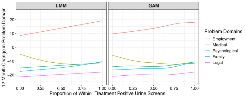
Figure 1: Fitted curves for the relationships between within-treatment frequency of cocaine use and changes in the 5 problem domains based on the unconstrained proposed model (LMM) and GAM.

We also visualized the fitted curves for all five problem domains as functions of within-treatment frequency of cocaine from our LMM approach (Fig. 1, left) as well as from GAM (Fig. 1, right). These curves were generated at the fixed reference levels of treatment group and study site while the values of baseline assessment of problem domains were all fixed at the mean across all domains and all subjects. Note that the resulting curves from LMM approach were based on REML, instead of ML, fit to the mixed effects model; although ML must be used for constructing LR test, REML can be used for estimation of the fitted curves. The estimated smoothing curves of each problem domain from both approaches are very similar. The curves from GAM tend to be more nonlinear. For the two domains (Employment and Family) with statistically significant associations with within-treatment frequency of cocaine use, both plots indicate that a 50% difference in within-treatment frequency of cocaine use, say 75% use versus 25% use, is associated with an approximate 5.5 point mean increase in employment problems and 2.5 point mean increase in family problems.

6 Discussion

In many applications, the relationship between the mean of an outcome and a quantitative covariate is complex and cannot be described by simple parametric functions (e.g., polynomial trends). In these settings, flexible nonlinear relationships can be incorporated using penalized splines. In this paper we have focused on the application of penalized splines in joint models that allow flexible nonlinear relationships for multiple outcomes. Due to the additional complexity of multiple correlated outcomes, the fitting of joint penalized spline models is potentially very challenging. We overcome this challenge by exploiting the known connection between penalized spline models and linear mixed effects models (e.g., Ruppert ., 2003). The linear mixed effects model representation simplifies model fitting in the multivariate outcome setting, and can also be implemented in existing statistical software, while allowing flexible nonlinear relationships with each outcome and properly accounting for the correlation among the outcomes. However, statistical inference based on a joint test of zero-effect of the quantitative covariate on the multiple outcomes involves testing that the variance components associated with each outcome are jointly equal to 0. When testing that a variance component equals 0, it is well-known that the usual asymptotic chi-square distribution of the likelihood ratio (LR) test under the null does not hold (Miller, 1977; Lin, 1997; Verbeke  Molenberghs, 2003). To overcome this limitation, we have proposed three permutation tests for the likelihood ratio test statistic; one based on permuting the quantitative covariate, the other two based on permuting residuals. Thus, the main contribution of this paper to methodology is that we have proposed an extension of the permutation approach to jointly test flexible nonlinear relationships, incorporated using penalized splines, to the multivariate setting with multiple outcomes. This includes a natural extension of the Cholesky residual permutation approach of Lee  Braun (2012) to multivariate outcomes.

Results from the simulation study lead to the following general recommendation concerning the three permutation tests we have proposed. A permutation test, based on permuting either the covariate or the vector of residuals, provides a robust alternative to the commonly used parametric GAM test proposed by Wood (2013), albeit with lower power for many alternatives where the parametric test appears valid. We note that for the case of non-normal errors, the permutation test based on Cholesky residuals had inflated Type I error rate and seemed less robust to non-normal errors. Similarly, the parametric test was found to have highly inflated Type I error rate with non-normal errors, suggesting this test is very sensitive to violations of distributional assumptions.

Finally, we note that the presentation of penalized splines, and our proposed permutation tests, has been for the special case of a simple piecewise linear spline. This focus on piecewise linear splines was primarily for notational convenience; all of the proposed tests generalize in a natural way to more flexible piecewise polynomial response models using alternative basis functions such as cubic splines and B-splines. For example, for cubic splines, the proposed $2K$ parameter joint tests simply become $4K$ parameter tests. The proposed permutation tests are not any more difficult to implement when other basis functions have been adopted. In addition, the focus of this paper has been on linear models for $K$ quantitative or continuous outcomes. However, we note that the proposed permutation tests can equally be applied in penalized splines for generalized linear models, e.g., logistic regression models. That is, the permutation tests can be implemented using a generalized linear mixed model (GLMM) representation of penalized splines; this is a topic of further research. In closing, we note that specification of penalized splines for multiple outcomes using the linear mixed effects model representation is straightforward to implement in widely available software for fitting linear mixed effects models. Obtaining permutation p-values for the proposed joint tests requires only modest additional programming; an R function for implementing the proposed permutation tests is included in the online appendix.

SUPPLEMENTARY MATERIAL

A written supplementary material contains additional results on Type I error and power in simulations, illustrating confidence intervals and impact of number of knots $C$, and for smaller sample size $N=50$. The R code for simulations and data application is provided as a separate zip file.

Table 1: Results for Type I error (Null) and power from simulations when $\epsilon_{ik}\sim\sqrt{1-\rho}\cdot\mathcal{N}(0,1)$ in equation (6). GAM stands for the parametric GAM test.

$(N,K)$	Methods	$\rho=0.25$				$\rho=0.75$      [b]
		Null	Sparse	Non-unif	Uniform	Null	Sparse	Non-unif	Uniform
$(200,5)$	Residual	.053	.152	.469	.707	.051	.712	.926	.437 [t]
	Covariate	.056	.153	.460	.701	.053	.713	.927	.431
	Cholesky	.053	.149	.466	.713	.050	.717	.927	.437
	GAM	.064	.554	.918	.965	.073	.976	.997	.181 [b]
$(100,5)$	Residual	.049	.096	.155	.386	.050	.271	.428	.244 [t]
	Covariate	.051	.091	.157	.383	.050	.271	.430	.247
	Cholesky	.049	.096	.151	.381	.052	.274	.438	.242
	GAM	.057	.258	.547	.616	.075	.700	.887	.140 [b]
$(100,10)$	Residual	.039	.089	.188	.280	.052	.229	.635	.182 [t]
	Covariate	.039	.089	.192	.278	.055	.232	.633	.186
	Cholesky	.039	.092	.188	.280	.055	.229	.633	.173
	GAM	.064	.206	.520	.210	.070	.704	.968	.093

Table 2: Results for Type I error (Null) and power from simulations when $\epsilon_{ik}\sim\sqrt{1-\rho}\cdot\text{SLN}(0,1)$ in equation (6). GAM stands for the parametric GAM test.

$(N,K)$	Methods	$\rho=0.25$				$\rho=0.75$      [b]
		Null	Sparse	Non-unif	Uniform	Null	Sparse	Non-unif	Uniform
$(200,5)$	Residual	.052	.141	.372	.597	.052	.633	.816	.319 [t]
	Covariate	.054	.139	.374	.586	.054	.629	.812	.311
	Cholesky	.061	.149	.390	.648	.067	.687	.865	.388
	GAM	.193	.622	.918	.921	.186	.979	.996	.264 [b]
$(100,5)$	Residual	.053	.075	.119	.229	.052	.262	.411	.151 [t]
	Covariate	.051	.074	.120	.234	.053	.259	.409	.145
	Cholesky	.064	.085	.137	.287	.073	.307	.471	.196
	GAM	.215	.391	.641	.561	.199	.774	.909	.213 [b]
$(100,10)$	Residual	.051	.074	.089	.097	.047	.153	.368	.068 [t]
	Covariate	.051	.066	.089	.083	.050	.161	.368	.070
	Cholesky	.063	.087	.124	.147	.092	.228	.493	.150
	GAM	.337	.474	.692	.453	.341	.812	.962	.382

Table 3: Univariate and joint tests of associations between problem domains and frequency of cocaine use. The p-values of univariate tests are not corrected for multiple comparisons. We only report results from the Cholesky residual permutation approach for the residual-based joint permutation test. For univariate tests, permuting Cholesky residuals is equivalent to permuting residuals directly. For the parametric GAM test, we use the Bonferroni corrected smallest univariate p-value as the p-value of the joint test.

	Permutation		GAM [b]
	Covariate	Residual
Employment	.0077	.0051	.0008 [t]
Medical	.2017	.1972	.0743
Psychological	.1135	.1164	.2995
Family	.0004	.0004	.0078
Legal	.0639	.0674	.1472 [b]
Joint	.0008	.0015	.0042 [t]

References

- American Psychiatric Association (\APACyear2000) \APACinsertmetastarassociation2000diagnostic{APACrefauthors}American Psychiatric Association. \APACrefYear2000. \APACrefbtitleDiagnostic and Statistical Manual of Mental Disorders, 4th Edition, Text Revision (DSM-IV-TR): Diagnostic and statistical manual of mental disorders, 4th edition, text revision (dsm-iv-tr):. \APACaddressPublisherAmerican Psychiatric Association. {APACrefURL} \urlhttps://books.google.com/books?id=_w5-BgAAQBAJ \PrintBackRefs\CurrentBib
- Anderson \BBA Legendre (\APACyear1999) \APACinsertmetastarandersonandlegendre{APACrefauthors}Anderson, M\BPBIJ.\BCBT \BBA Legendre, P. \APACrefYearMonthDay1999. \BBOQ\APACrefatitleAn empirical comparison of permutation methods for tests of partial regression coefficients in a linear model An empirical comparison of permutation methods for tests of partial regression coefficients in a linear model.\BBCQ \APACjournalVolNumPagesJournal of Statistical Computation and Simulation623271-303. {APACrefURL} \urlhttps://doi.org/10.1080/00949659908811936 {APACrefDOI} 10.1080/00949659908811936 \PrintBackRefs\CurrentBib
- Bubeliny (\APACyear2010) \APACinsertmetastarbubeliny2010hotelling{APACrefauthors}Bubeliny, P. \APACrefYearMonthDay2010. \BBOQ\APACrefatitleHotelling’s test for highly correlated data Hotelling’s test for highly correlated data.\BBCQ \APACjournalVolNumPagesarXiv preprint arXiv:1007.1094. \PrintBackRefs\CurrentBib
- Chen \BBA Wang (\APACyear2011) \APACinsertmetastarchen2011penalized{APACrefauthors}Chen, H.\BCBT \BBA Wang, Y. \APACrefYearMonthDay2011. \BBOQ\APACrefatitleA penalized spline approach to functional mixed effects model analysis A penalized spline approach to functional mixed effects model analysis.\BBCQ \APACjournalVolNumPagesBiometrics673861–870. \PrintBackRefs\CurrentBib
- Chen \BOthers. (\APACyear2013) \APACinsertmetastarchen2013marginal{APACrefauthors}Chen, H., Wang, Y., Paik, M\BPBIC.\BCBL \BBA Choi, H\BPBIA. \APACrefYearMonthDay2013. \BBOQ\APACrefatitleA marginal approach to reduced-rank penalized spline smoothing with application to multilevel functional data A marginal approach to reduced-rank penalized spline smoothing with application to multilevel functional data.\BBCQ \APACjournalVolNumPagesJournal of the American Statistical Association1085041216–1229. \PrintBackRefs\CurrentBib
- Crainiceanu \BBA Ruppert (\APACyear2004\APACexlab\BCnt1) \APACinsertmetastarCRAINICEANU200435{APACrefauthors}Crainiceanu, C\BPBIM.\BCBT \BBA Ruppert, D. \APACrefYearMonthDay2004\BCnt1. \BBOQ\APACrefatitleLikelihood ratio tests for goodness-of-fit of a nonlinear regression model Likelihood ratio tests for goodness-of-fit of a nonlinear regression model.\BBCQ \APACjournalVolNumPagesJournal of Multivariate Analysis91135-52. {APACrefURL} \urlhttps://www.sciencedirect.com/science/article/pii/S0047259X0400082X {APACrefDOI} https://doi.org/10.1016/j.jmva.2004.04.008 \PrintBackRefs\CurrentBib
- Crainiceanu \BBA Ruppert (\APACyear2004\APACexlab\BCnt2) \APACinsertmetastarcrainiceanu2004likelihood{APACrefauthors}Crainiceanu, C\BPBIM.\BCBT \BBA Ruppert, D. \APACrefYearMonthDay2004\BCnt2. \BBOQ\APACrefatitleLikelihood ratio tests in linear mixed models with one variance component Likelihood ratio tests in linear mixed models with one variance component.\BBCQ \APACjournalVolNumPagesJournal of the Royal Statistical Society: Series B (Statistical Methodology)661165–185. \PrintBackRefs\CurrentBib
- Crainiceanu \BOthers. (\APACyear2002) \APACinsertmetastarcrainiceanu2002probability{APACrefauthors}Crainiceanu, C\BPBIM., Ruppert, D.\BCBL \BBA Vogelsang, T. \APACrefYearMonthDay2002. \BBOQ\APACrefatitleProbability that the MLE of a variance component is zero with applications to likelihood ratio tests Probability that the mle of a variance component is zero with applications to likelihood ratio tests.\BBCQ \APACjournalVolNumPagesUnpublished manuscript. \PrintBackRefs\CurrentBib
- Craven \BBA Wahba (\APACyear1978) \APACinsertmetastarcraven_smoothing_1978{APACrefauthors}Craven, P.\BCBT \BBA Wahba, G. \APACrefYearMonthDay1978. \BBOQ\APACrefatitleSmoothing noisy data with spline functions Smoothing noisy data with spline functions.\BBCQ \APACjournalVolNumPagesNumerische Mathematik314377–403. {APACrefURL} \urlhttps://doi.org/10.1007/BF01404567 {APACrefDOI} 10.1007/BF01404567 \PrintBackRefs\CurrentBib
- Crits-Christoph \BOthers. (\APACyear1999) \APACinsertmetastarcrits1999psychosocial{APACrefauthors}Crits-Christoph, P., Siqueland, L., Blaine, J., Frank, A., Luborsky, L., Onken, L\BPBIS.\BDBLothers \APACrefYearMonthDay1999. \BBOQ\APACrefatitlePsychosocial treatments for cocaine dependence: National Institute on Drug Abuse collaborative cocaine treatment study Psychosocial treatments for cocaine dependence: National institute on drug abuse collaborative cocaine treatment study.\BBCQ \APACjournalVolNumPagesArchives of General Psychiatry566493–502. \PrintBackRefs\CurrentBib
- DiCiccio \BBA Romano (\APACyear2017) \APACinsertmetastardiciccio2017robust{APACrefauthors}DiCiccio, C\BPBIJ.\BCBT \BBA Romano, J\BPBIP. \APACrefYearMonthDay2017. \BBOQ\APACrefatitleRobust permutation tests for correlation and regression coefficients Robust permutation tests for correlation and regression coefficients.\BBCQ \APACjournalVolNumPagesJournal of the American Statistical Association1125191211–1220. \PrintBackRefs\CurrentBib
- Draper \BBA Stoneman (\APACyear1966) \APACinsertmetastardraper1966testing{APACrefauthors}Draper, N\BPBIR.\BCBT \BBA Stoneman, D\BPBIM. \APACrefYearMonthDay1966. \BBOQ\APACrefatitleTesting for the inclusion of variables in einear regression by a randomisation technique Testing for the inclusion of variables in einear regression by a randomisation technique.\BBCQ \APACjournalVolNumPagesTechnometrics84695–699. \PrintBackRefs\CurrentBib
- Drikvandi \BOthers. (\APACyear2013) \APACinsertmetastardrikvandi2013testing{APACrefauthors}Drikvandi, R., Verbeke, G., Khodadadi, A.\BCBL \BBA Partovi Nia, V. \APACrefYearMonthDay2013. \BBOQ\APACrefatitleTesting multiple variance components in linear mixed-effects models Testing multiple variance components in linear mixed-effects models.\BBCQ \APACjournalVolNumPagesBiostatistics141144–159. \PrintBackRefs\CurrentBib
- Du \BBA Wang (\APACyear2020) \APACinsertmetastardu2020testing{APACrefauthors}Du, H.\BCBT \BBA Wang, L. \APACrefYearMonthDay2020. \BBOQ\APACrefatitleTesting variance components in linear mixed modeling using permutation Testing variance components in linear mixed modeling using permutation.\BBCQ \APACjournalVolNumPagesMultivariate behavioral research551120–136. \PrintBackRefs\CurrentBib
- Fitzmaurice \BOthers. (\APACyear2012) \APACinsertmetastarfitzmaurice2012applied{APACrefauthors}Fitzmaurice, G\BPBIM., Laird, N\BPBIM.\BCBL \BBA Ware, J\BPBIH. \APACrefYear2012. \APACrefbtitleApplied longitudinal analysis Applied longitudinal analysis. \APACaddressPublisherJohn Wiley & Sons. \PrintBackRefs\CurrentBib
- Freedman \BBA Lane (\APACyear1983) \APACinsertmetastarfreedmanandlane{APACrefauthors}Freedman, D.\BCBT \BBA Lane, D. \APACrefYearMonthDay1983. \BBOQ\APACrefatitleA Nonstochastic Interpretation of Reported Significance Levels A nonstochastic interpretation of reported significance levels.\BBCQ \APACjournalVolNumPagesJournal of Business & Economic Statistics14292-298. {APACrefURL} \urlhttps://www.tandfonline.com/doi/abs/10.1080/07350015.1983.10509354 {APACrefDOI} 10.1080/07350015.1983.10509354 \PrintBackRefs\CurrentBib
- Henderson (\APACyear1975) \APACinsertmetastarhenderson1975best{APACrefauthors}Henderson, C\BPBIR. \APACrefYearMonthDay1975. \BBOQ\APACrefatitleBest linear unbiased estimation and prediction under a selection model Best linear unbiased estimation and prediction under a selection model.\BBCQ \APACjournalVolNumPagesBiometrics423–447. \PrintBackRefs\CurrentBib
- Lee \BBA Braun (\APACyear2012) \APACinsertmetastarlee2012permutation{APACrefauthors}Lee, O\BPBIE.\BCBT \BBA Braun, T\BPBIM. \APACrefYearMonthDay2012. \BBOQ\APACrefatitlePermutation tests for random effects in linear mixed models Permutation tests for random effects in linear mixed models.\BBCQ \APACjournalVolNumPagesBiometrics682486–493. \PrintBackRefs\CurrentBib
- Lin (\APACyear1997) \APACinsertmetastarlin1997variance{APACrefauthors}Lin, X. \APACrefYearMonthDay1997. \BBOQ\APACrefatitleVariance component testing in generalised linear models with random effects Variance component testing in generalised linear models with random effects.\BBCQ \APACjournalVolNumPagesBiometrika842309–326. \PrintBackRefs\CurrentBib
- Manly (\APACyear2018) \APACinsertmetastarmanly2018randomization{APACrefauthors}Manly, B\BPBIF. \APACrefYear2018. \APACrefbtitleRandomization, bootstrap and Monte Carlo methods in biology Randomization, bootstrap and monte carlo methods in biology. \APACaddressPublisherChapman and Hall/CRC. \PrintBackRefs\CurrentBib
- McLellan \BOthers. (\APACyear1992) \APACinsertmetastarmclellan1992fifth{APACrefauthors}McLellan, A\BPBIT., Kushner, H., Metzger, D., Peters, R., Smith, I., Grissom, G.\BDBLArgeriou, M. \APACrefYearMonthDay1992. \BBOQ\APACrefatitleThe fifth edition of the Addiction Severity Index The fifth edition of the addiction severity index.\BBCQ \APACjournalVolNumPagesJournal of Substance Abuse Treatment93199–213. \PrintBackRefs\CurrentBib
- Miller (\APACyear1977) \APACinsertmetastarmiller1977asymptotic{APACrefauthors}Miller, J\BPBIJ. \APACrefYearMonthDay1977. \BBOQ\APACrefatitleAsymptotic properties of maximum likelihood estimates in the mixed model of the analysis of variance Asymptotic properties of maximum likelihood estimates in the mixed model of the analysis of variance.\BBCQ \APACjournalVolNumPagesThe Annals of Statistics746–762. \PrintBackRefs\CurrentBib
- Pesarin \BBA Salmaso (\APACyear2010) \APACinsertmetastarpesarin2010permutation{APACrefauthors}Pesarin, F.\BCBT \BBA Salmaso, L. \APACrefYear2010. \APACrefbtitlePermutation tests for complex data: theory, applications and software Permutation tests for complex data: theory, applications and software. \APACaddressPublisherJohn Wiley & Sons. \PrintBackRefs\CurrentBib
- R Core Team (\APACyear2019) \APACinsertmetastarrman{APACrefauthors}R Core Team. \APACrefYearMonthDay2019. \BBOQ\APACrefatitleR: A Language and Environment for Statistical Computing R: A language and environment for statistical computing\BBCQ [\bibcomputersoftwaremanual]. \APACaddressPublisherVienna, Austria. {APACrefURL} \urlhttps://www.R-project.org/ \PrintBackRefs\CurrentBib
- Raz (\APACyear1990) \APACinsertmetastarraz{APACrefauthors}Raz, J. \APACrefYearMonthDay1990. \BBOQ\APACrefatitleTesting for No Effect When Estimating a Smooth Function by Nonparametric Regression: A Randomization Approach Testing for no effect when estimating a smooth function by nonparametric regression: A randomization approach.\BBCQ \APACjournalVolNumPagesJournal of the American Statistical Association85409132-138. {APACrefURL} \urlhttps://www.tandfonline.com/doi/abs/10.1080/01621459.1990.10475316 {APACrefDOI} 10.1080/01621459.1990.10475316 \PrintBackRefs\CurrentBib
- Ruppert \BOthers. (\APACyear2003) \APACinsertmetastarruppert2003semiparametric{APACrefauthors}Ruppert, D., Wand, M\BPBIP.\BCBL \BBA Carroll, R\BPBIJ. \APACrefYear2003. \APACrefbtitleSemiparametric regression Semiparametric regression. \APACaddressPublisherCambridge University Press. \PrintBackRefs\CurrentBib
- Samuh \BOthers. (\APACyear2012) \APACinsertmetastarsamuh2012use{APACrefauthors}Samuh, M\BPBIH., Grilli, L., Rampichini, C., Salmaso, L.\BCBL \BBA Lunardon, N. \APACrefYearMonthDay2012. \BBOQ\APACrefatitleThe use of permutation tests for variance components in linear mixed models The use of permutation tests for variance components in linear mixed models.\BBCQ \APACjournalVolNumPagesCommunications in Statistics-Theory and Methods4116-173020–3029. \PrintBackRefs\CurrentBib
- SAS Institute Inc. (\APACyear2015) \APACinsertmetastarSAS-STAT{APACrefauthors}SAS Institute Inc. \APACrefYearMonthDay2015. \BBOQ\APACrefatitleSAS/STAT Software, Version 9.4 Sas/stat software, version 9.4\BBCQ [\bibcomputersoftwaremanual]. \APACaddressPublisherCary, NC. {APACrefURL} \urlhttp://www.sas.com/ \PrintBackRefs\CurrentBib
- Scheipl \BOthers. (\APACyear2008) \APACinsertmetastarSCHEIPL20083283{APACrefauthors}Scheipl, F., Greven, S.\BCBL \BBA Küchenhoff, H. \APACrefYearMonthDay2008. \BBOQ\APACrefatitleSize and power of tests for a zero random effect variance or polynomial regression in additive and linear mixed models Size and power of tests for a zero random effect variance or polynomial regression in additive and linear mixed models.\BBCQ \APACjournalVolNumPagesComputational Statistics & Data Analysis5273283-3299. {APACrefURL} \urlhttps://www.sciencedirect.com/science/article/pii/S0167947307004306 {APACrefDOI} https://doi.org/10.1016/j.csda.2007.10.022 \PrintBackRefs\CurrentBib
- Self \BBA Liang (\APACyear1987) \APACinsertmetastarself1987asymptotic{APACrefauthors}Self, S\BPBIG.\BCBT \BBA Liang, K\BHBIY. \APACrefYearMonthDay1987. \BBOQ\APACrefatitleAsymptotic properties of maximum likelihood estimators and likelihood ratio tests under nonstandard conditions Asymptotic properties of maximum likelihood estimators and likelihood ratio tests under nonstandard conditions.\BBCQ \APACjournalVolNumPagesJournal of the American Statistical Association82398605–610. \PrintBackRefs\CurrentBib
- Shapiro (\APACyear1985) \APACinsertmetastarshapiro1985asymptotic{APACrefauthors}Shapiro, A. \APACrefYearMonthDay1985. \BBOQ\APACrefatitleAsymptotic distribution of test statistics in the analysis of moment structures under inequality constraints Asymptotic distribution of test statistics in the analysis of moment structures under inequality constraints.\BBCQ \APACjournalVolNumPagesBiometrika721133–144. \PrintBackRefs\CurrentBib
- Stoel \BOthers. (\APACyear2006) \APACinsertmetastarstoel2006likelihood{APACrefauthors}Stoel, R\BPBID., Garre, F\BPBIG., Dolan, C.\BCBL \BBA Van Den Wittenboer, G. \APACrefYearMonthDay2006. \BBOQ\APACrefatitleOn the likelihood ratio test in structural equation modeling when parameters are subject to boundary constraints. On the likelihood ratio test in structural equation modeling when parameters are subject to boundary constraints.\BBCQ \APACjournalVolNumPagesPsychological Methods114439. \PrintBackRefs\CurrentBib
- Stram \BBA Lee (\APACyear1994) \APACinsertmetastarstram1994variance{APACrefauthors}Stram, D\BPBIO.\BCBT \BBA Lee, J\BPBIW. \APACrefYearMonthDay1994. \BBOQ\APACrefatitleVariance components testing in the longitudinal mixed effects model Variance components testing in the longitudinal mixed effects model.\BBCQ \APACjournalVolNumPagesBiometrics1171–1177. \PrintBackRefs\CurrentBib
- Verbeke \BBA Molenberghs (\APACyear2003) \APACinsertmetastarverbeke2003use{APACrefauthors}Verbeke, G.\BCBT \BBA Molenberghs, G. \APACrefYearMonthDay2003. \BBOQ\APACrefatitleThe use of score tests for inference on variance components The use of score tests for inference on variance components.\BBCQ \APACjournalVolNumPagesBiometrics592254–262. \PrintBackRefs\CurrentBib
- Wang (\APACyear1998\APACexlab\BCnt1) \APACinsertmetastarwang1998mixed{APACrefauthors}Wang, Y. \APACrefYearMonthDay1998\BCnt1. \BBOQ\APACrefatitleMixed effects smoothing spline analysis of variance Mixed effects smoothing spline analysis of variance.\BBCQ \APACjournalVolNumPagesJournal of the Royal Statistical Society: Series B (Statistical Methodology)601159–174. \PrintBackRefs\CurrentBib
- Wang (\APACyear1998\APACexlab\BCnt2) \APACinsertmetastarwang1998smoothing{APACrefauthors}Wang, Y. \APACrefYearMonthDay1998\BCnt2. \BBOQ\APACrefatitleSmoothing spline models with correlated random errors Smoothing spline models with correlated random errors.\BBCQ \APACjournalVolNumPagesJournal of the American Statistical Association93441341–348. \PrintBackRefs\CurrentBib
- Winkler \BOthers. (\APACyear2014) \APACinsertmetastarWINKLER2014381{APACrefauthors}Winkler, A\BPBIM., Ridgway, G\BPBIR., Webster, M\BPBIA., Smith, S\BPBIM.\BCBL \BBA Nichols, T\BPBIE. \APACrefYearMonthDay2014. \BBOQ\APACrefatitlePermutation inference for the general linear model Permutation inference for the general linear model.\BBCQ \APACjournalVolNumPagesNeuroImage92381-397. {APACrefURL} \urlhttps://www.sciencedirect.com/science/article/pii/S1053811914000913 {APACrefDOI} https://doi.org/10.1016/j.neuroimage.2014.01.060 \PrintBackRefs\CurrentBib
- Wood (\APACyear2003) \APACinsertmetastarwood2003thin{APACrefauthors}Wood, S\BPBIN. \APACrefYearMonthDay2003. \BBOQ\APACrefatitleThin plate regression splines Thin plate regression splines.\BBCQ \APACjournalVolNumPagesJournal of the Royal Statistical Society: Series B (Statistical Methodology)65195–114. \PrintBackRefs\CurrentBib
- Wood (\APACyear2013) \APACinsertmetastarwood2013p{APACrefauthors}Wood, S\BPBIN. \APACrefYearMonthDay2013. \BBOQ\APACrefatitleOn p-values for smooth components of an extended generalized additive model On p-values for smooth components of an extended generalized additive model.\BBCQ \APACjournalVolNumPagesBiometrika1001221–228. \PrintBackRefs\CurrentBib
- Wood (\APACyear2015) \APACinsertmetastarwood2015package{APACrefauthors}Wood, S\BPBIN. \APACrefYearMonthDay2015. \BBOQ\APACrefatitlePackage ‘mgcv’ Package ‘mgcv’.\BBCQ \APACjournalVolNumPagesR package version129. \PrintBackRefs\CurrentBib
- Wu \BBA Neale (\APACyear2013) \APACinsertmetastarwu2013likelihood{APACrefauthors}Wu, H.\BCBT \BBA Neale, M\BPBIC. \APACrefYearMonthDay2013. \BBOQ\APACrefatitleOn the likelihood ratio tests in bivariate ACDE models On the likelihood ratio tests in bivariate acde models.\BBCQ \APACjournalVolNumPagesPsychometrika783441–463. \PrintBackRefs\CurrentBib
- Yoon \BOthers. (\APACyear2011) \APACinsertmetastaryoon2011alternative{APACrefauthors}Yoon, F\BPBIB., Fitzmaurice, G\BPBIM., Lipsitz, S\BPBIR., Horton, N\BPBIJ., Laird, N\BPBIM.\BCBL \BBA Normand, S\BHBIL\BPBIT. \APACrefYearMonthDay2011. \BBOQ\APACrefatitleAlternative methods for testing treatment effects on the basis of multiple outcomes: simulation and case study Alternative methods for testing treatment effects on the basis of multiple outcomes: simulation and case study.\BBCQ \APACjournalVolNumPagesStatistics in Medicine30161917–1932. \PrintBackRefs\CurrentBib