Toric 2-group anomalies via cobordism

Abstract

2-group symmetries arise in physics when a 0-form symmetry $G^{[0]}$ and a 1-form symmetry $H^{[1]}$ intertwine, forming a generalised group-like structure. Specialising to the case where both $G^{[0]}$ and $H^{[1]}$ are compact, connected, abelian groups (i.e. tori), we analyse anomalies in such ‘toric 2-group symmetries’ using the cobordism classification. As a warm up example, we use cobordism to study various ’t Hooft anomalies (and the phases to which they are dual) in Maxwell theory defined on non-spin manifolds. For our main example, we compute the 5th spin bordism group of $B|\mathbb{G}|$ where $\mathbb{G}$ is any 2-group whose 0-form and 1-form symmetry parts are both $\mathrm{U}(1)$, and $|\mathbb{G}|$ is the geometric realisation of the nerve of the 2-group $\mathbb{G}$. By leveraging a variety of algebraic methods, we show that $\Omega^{\mathrm{Spin}}_{5}(B|\mathbb{G}|)\cong\mathbb{Z}/m$ where $m$ is the modulus of the Postnikov class for $\mathbb{G}$, and we reproduce the expected physics result for anomalies in 2-group symmetries that appear in 4d QED. Moving down two dimensions, we recap that any (anomalous) $\mathrm{U}(1)$ global symmetry in 2d can be enhanced to a toric 2-group symmetry, before showing that its associated local anomaly reduces to at most an order 2 anomaly, when the theory is defined with a spin structure.

1 Introduction

In quantum field theory, anomalies are loosely defined to be quantum obstructions to symmetries. More precisely, anomalies can themselves be identified with (special classes of) quantum field theories in one dimension higher than the original theory, via the idea of ‘anomaly inflow’. This modern viewpoint led to an algebraic classification of anomalies via cobordism, which was made rigorous by Freed and Hopkins Freed:2016rqq following many important works (including Witten:1985xe ; Dai:1994kq ; Kapustin:2014dxa ; Witten:2015aba ; Witten:2019bou ). The cobordism classification includes all known anomalies afflicting chiral symmetries of massless fermions in any number of dimensions, as well as other more subtle anomalies that involve discrete spacetime symmetries (see e.g. Tachikawa:2018njr ; Witten:2016cio ; Wang:2018qoy ).

The cobordism group that classifies anomalies, for $d$ spacetime dimensions and symmetry type $\SS$, is the Anderson dual of bordism Freed:2016rqq ,

$$H_{I\mathbb{Z}}^{d+2}\left(MT\SS\right):=[MT\SS,\Sigma^{d+2}I\mathbb{Z}],$$ (1.1)

where $MT\SS$ denotes the Madsen–Tillman spectrum associated to symmetry type $\SS$, $I\mathbb{Z}$ denotes the Anderson dual of the sphere spectrum (with $\Sigma^{d+2}$ denoting the $d+2$-fold suspension), and $[X,Y]$ denotes the homotopy classes of maps between a pair of spectra $X$ and $Y$. In fact, this cobordism classification goes beyond what we would normally think of as ‘anomalies’ to cover all reflection positive invertible field theories (with or without fermions) with symmetry $\SS$ in $d+1$-dimensions.

To unpack the meaning and significance of the cobordism group $H_{I\mathbb{Z}}^{d+2}\left(MT\SS\right)$, it is helpful to recall that it fits inside a defining short exact sequence Freed:2016rqq

$$\text{Ext}^{1}_{\mathbb{Z}}\left(\pi_{d+1}(MT\SS),\mathbb{Z}\right)\hookrightarrow H_{I\mathbb{Z}}^{d+2}\left(MT\SS\right)\twoheadrightarrow\operatorname*{Hom}\left(\pi_{d+2}(MT\SS),\mathbb{Z}\right),$$ (1.2)

where $\pi_{k}(X)$ is the $k^{\text{th}}$ stable homotopy group of a spectrum $X$. For the special case of chiral fermion anomalies in $d$ dimensions, the invertible field theory in question is precisely the exponentiated $\eta$-invariant Witten:2019bou of Atiyah, Patodi and Singer Atiyah:1975jf ; Atiyah:1976jg ; Atiyah:1976qjr in dimension $d+1$. In that case, integrating the gauge-invariant anomaly polynomial $\Phi_{d+2}$ provides an element of the right factor $\operatorname*{Hom}\left(\pi_{d+2}(MT\SS),\mathbb{Z}\right)$. Theories with $\Phi_{d+2}=0$, which are in the kernel of the right map and thus in the image of the left map, correspond to residual ‘global anomalies’ which are thus captured by the left-factor. For theories with symmetry type $\SS=\text{Spin}\times G$, where $G$ is the internal symmetry group, we have that $\text{Ext}^{1}_{\mathbb{Z}}\left(\pi_{d+1}(MT\SS),\mathbb{Z}\right)\cong\operatorname*{Hom}\left(\operatorname*{Tor}\Omega_{d+1}^{\text{Spin}}(BG),\mathbb{R}/\mathbb{Z}\right)$ classifies global anomalies, where $\Omega_{\bullet}^{\text{Spin}}$ denotes spin bordism. A straightforward corollary is that if the group $\operatorname*{Tor}\Omega_{d+1}^{\text{Spin}}(BG)$ vanishes there can be no global anomalies, which has been applied to various particle physics applications in recent years Freed:2006mx ; Garcia-Etxebarria:2017crf ; Garcia-Etxebarria:2018ajm ; Wan:2018bns ; Seiberg:2018ntt ; Hsieh:2019iba ; Davighi:2019rcd ; Wan:2019gqr ; Davighi:2020uab ; Lee:2020ewl ; Davighi:2020kok ; Debray:2021vob ; Davighi:2022fer ; Davighi:2022bqf ; Wang:2022eag ; Lee:2022spd ; Davighi:2022icj ; Debray:2023yrs .

Concurrent with this development of the cobordism classification of anomalies, in the past decade the notion of ‘symmetry’ has been generalised beyond the action of groups on local operators, in various exciting directions (for recent reviews, see Ref. Cordova:2022ruw ; Bah:2022wot ). This includes the notion of $p$-form symmetries Gaiotto:2014kfa , which act not on local operators (the case $p=0$) but more generally on extended operators of dimension $p$. These symmetries couple to background fields that are $(p+1)$-form gauge fields. Such higher-form symmetries are found in a plethora of quantum field theories. The most well-known examples include a pair of $\text{U}(1)$ 1-form symmetries in 4d Maxwell theory, and a $\mathbb{Z}/N$ 1-form symmetry in 4d $\text{SU}(N)$ Yang–Mills theory; the latter exhibits a mixed anomaly with charge-parity symmetry when the $\text{SU}(N)$ $\theta$-angle equals $\pi$, which led to new insights regarding the vacua of QCD Gaiotto:2017yup . Other important classes of generalised symmetry include non-invertible and categorical symmetries, as well as subsystem symmetries. These shall play no role in the present paper.

Soon after the notion of $p$-form symmetries was formalised in Gaiotto:2014kfa , it was realised that higher-form symmetries of different degrees can ‘mix’, leading to the notion of $p$-group symmetry. The most down-to-earth example of this symmetry structure, which in general is described using higher category theory (see e.g. Gripaios:2022yjy ), is the notion of a 2-group symmetry whereby a 1-form symmetry $H^{[1]}$ and a 0-form symmetry $G^{[0]}$ combine non-trivially. This occurs, for example Hsin:2020nts ; Lee:2021crt , when a bunch of Wilson lines (which are charged under a discrete 1-form centre symmetry) can be screened by a dynamical fermion (which is charged under a 0-form flavour symmetry). 2-group symmetries were first observed, in their gauged form, in string theory in the context of the Green–Schwarz mechanism, in which a $\text{U}(1)$ 1-form symmetry combines non-trivially with a diffeomorphism Baez:2005sn ; Sati:2009ic ; Fiorenza:2010mh ; Fiorenza:2012tb . Their appearance as global symmetries in field theory was appreciated first by Sharpe Sharpe:2015mja , before many new examples were identified in Refs. Cordova:2018cvg ; Benini:2018reh . Further instances of 2-group symmetry have since been discovered and analysed in 4d Hsin:2020nts ; Lee:2021crt ; Bhardwaj:2021wif ; Cvetic:2022imb ; Carta:2022fxc , 5d Cvetic:2022imb ; Benini:2018reh ; Apruzzi:2021vcu ; DelZotto:2022fnw ; DelZotto:2022joo , and 6d Cordova:2020tij ; DelZotto:2020sop ; Apruzzi:2021mlh quantum field theories. A 2-group symmetry structure has recently been studied in the Standard Model Cordova:2022qtz , in the limit of zero Yukawa couplings.

In this paper we study how the cobordism classification of anomalies can be applied to 2-group symmetries. As a first step, we here specialise to 2-groups for which both $G^{[0]}$ and $H^{[1]}$ are compact, connected, abelian groups ergo tori $\cong\text{U}(1)^{n}$; we refer to such a structure, at times, as a ‘toric 2-group’. In this case, there are 1-form and 2-form Noether currents $j^{(1)}_{G}$ and $j^{(2)}_{H}$ associated with the 0-form and 1-form symmetries respectively, and the non-trivial 2-group ‘mixing’ between these symmetries is reflected in a fusion rule for these currents, schematically

$$j^{(1)}_{G}(x)j^{(1)}_{G}(0)\sim K(x)j^{(2)}_{H}(0)+\dots,$$ (1.3)

for a known (singular) function $K(x)$. Toric 2-group symmetries appear, for example, in chiral $\text{U}(1)$ gauge theories in 4d when there are mixed ‘operator-valued’ anomalies between global chiral symmetry currents and the gauge current Cordova:2018cvg , as well as in 3d Damia:2022rxw and in hydrodynamics Iqbal:2020lrt . Toric 2-group symmetries thus naturally appear in fermionic systems, for which anomalies can be more fruitfully analysed using cobordism (compared to purely bosonic anomalies).

For such a toric 2-group $\mathbb{G}$, we study the bordism theory of manifolds equipped with ‘tangential $\mathbb{G}$-structure’. This can be defined analogously to a tangential $\SS$-structure for ordinary symmetry type $\SS$, given now the particular 2-group $\mathbb{G}$ plus an appropriate form of spin structure. When the 2-group symmetry does not further mix with the spacetime symmetry, this reduces to studying the spin bordism groups of the topological space that classifies $\mathbb{G}$-2-bundles.

Thankfully much is known about the classifying space of $\mathbb{G}$-2-bundles that will be of use to us, given the physics applications we have in mind. Quite generally, the classifying space of a 2-group $\mathbb{G}$ can be computed as $B|\mathbb{G}|$, where $|\mathbb{G}|$ is the geometric realization of the nerve of the 2-group $\mathbb{G}$ viewed as a category bartels2006higher ; Baez2008 , which is itself a topological 1-group — albeit often an infinite-dimensional one. This means that Freed and Hopkins’ classification of invertible field theories with fixed symmetry type can be applied directly, taking the tangential structure to be $\text{Spin}\times|\mathbb{G}|$.

In the special case of a pure 1-form symmetry valued in an abelian group $H^{[1]}=A$, this formula for the classifying space of the corresponding 2-group reduces to $B(BA)$, recovering the well-known result for classifying abelian gerbes brylinski2007loop . This special case, which is of significant physical interest, has already been used in the physics literature to study 1-form anomalies, for many examples with variously Spin, SO, and O structures in Ref. Wan:2018bns . An extension of this to a pure 2-form symmetry and its anomalies in 6d gauge theories was studied via cobordism in Ref. Lee:2020ewl .

More generally for any 2-group $\mathbb{G}$, the classifying space $B|\mathbb{G}|$ always sits in a ‘defining fibration’

$$B\left(BH^{[1]}\right)\to B|\mathbb{G}|\to BG^{[0]}\,,$$ (1.4)

which allows one to leverage the usual spectral sequence methods to compute e.g. the cohomology and/or the (co)bordism groups of $B|\mathbb{G}|$. For ‘non-trivial’ 2-groups, i.e. those for which the fibration (1.4) is non-trivial, there is to our knowledge only a smattering of calculations in the literature; in particular, the case $B(B\mathbb{Z}/2^{[1]})\to B|\mathbb{G}|\to B\text{O}^{[0]}$ was studied by Wan and Wang Wan:2018bns (Section 4), and $B(B\text{U}(1)^{[1]})\to B|\mathbb{G}|\to B\text{SU}(2)^{[0]}$ was studied by Lee and Tachikawa Lee:2020ewl (Appendix B.6). In this paper we extend these works with a dedicated cobordism analysis of theories with 2-group symmetry and their anomalies.

The content of this paper is as follows. After reviewing 2-groups and their appearances in quantum field theory in §2, we then describe the topological spaces $B|\mathbb{G}|$ that classify 2-group background fields, and show how these spaces can be computed, in §3. By considering appropriate tangential structures for 2-group symmetries, this then leads to a definition of the cobordism groups relevant for describing 2-group symmetries and their anomalies (§3.2). We then apply this cobordism theory to study a small selection of examples in detail, focussing on toric 2-group symmetries as an especially tractable case. The main examples that we study in this paper are as follows. In §4, which is a warm up example, we study anomalies involving the pair of 1-form symmetries in 4d Maxwell theory, defined on non-spin manifolds. As well as the $\mathbb{Z}$-valued ‘local’ mixed anomaly between the two 1-form symmetries Gaiotto:2014kfa ; Wang-Senthil:2016a ; Hsin:2019fhf ; Brennan:2022tyl , there is a trio of $\mathbb{Z}/2$-valued global anomalies (involving gravity) that only appear on non-spin manifolds; the associated phases have been studied in Jian:2020qab . In §5 we turn to our main example of toric 2-group symmetries, with non-trivial Postnikov class, occurring in 4d abelian chiral theories. We see, using cobordism, how turning on the Postnikov class transmutes a $\mathbb{Z}$-valued local anomaly into a torsion-valued global anomaly à la the Green–Schwarz mechanism – we precisely recover the physics results derived by Córdova, Dumitrescu and Intriligator in Ref Cordova:2018cvg . Finally, in §6 we drop down to two dimensions, where anomalous 0-form symmetries can be recast as 2-group symmetries by using the trivially conserved 1-form symmetry whose 2-form current is simply the volume form Sharpe:2015mja . Our cobordism analysis highlights the prominent role played by spin structures; when the $\text{U}(1)^{[0]}$ anomaly coefficient is odd, the Green–Schwarz mechanism cannot in fact absorb the anomaly completely but leaves a $\mathbb{Z}/2$-valued anomaly, which we identify as an anomaly in the spin structure; we also show how this $\mathbb{Z}/2$-anomaly is trivialised upon passing to $\text{Spin}_{c}$ bordism.

2 Review: 2-groups and their classifying spaces

In this Section we recall the notion of a 2-group $\mathbb{G}$ (§2.1), and briefly reprise their appearance as generalised symmetry structures in quantum field theory (§2.2).

2.1 What is a 2-group?

We begin by sketching some equivalent definitions of a 2-group, for which our main reference is Ref. Baez2008 by Baez and Stevenson. First and most concise is probably the definition of a 2-group $\mathbb{G}$ as a higher category. Loosely, a 2-group $\mathbb{G}$ is in this language a 2-category that contains a single object, with all 1-morphisms and 2-morphisms being invertible.

(Slightly) less abstractly, a 2-group can also be described using ‘ordinary’ category theory, without recourse to higher categories, and this can be done in two ways; either as a groupoid in the category of groups, or as a group in the category of groupoids. Expanding on the former viewpoint, a 2-group is itself a category whose objects form a group $\tilde{G}^{[0]}$, and whose morphisms also form a group, where the latter can be written as a semi-direct product between $\tilde{G}^{[0]}$ and another group $\tilde{H}^{[1]}$, viz.

$$\operatorname*{Obj}(\mathbb{G})=\tilde{G}^{[0]},\qquad\operatorname*{Mor}(\mathbb{G})=\tilde{H}^{[1]}\rtimes\tilde{G}^{[0]},$$ (2.1)

such that all the various maps involved in the definition of a groupoid are continuous group homomorphisms (see §3 of Baez2008 ). We will usually be interested in situations where both $\tilde{G}^{[0]}$ and $\tilde{H}^{[1]}$ are Lie groups.

This definition involving a pair of groups $(\tilde{G}^{[0]},\tilde{H}^{[1]})$ is closely related to yet another, somewhat more practical, definition of a 2-group as a topological crossed module. The data specifying a topological crossed module consists of a quadruplet

$$\mathbb{G}=(\tilde{G}^{[0]},\tilde{H}^{[1]},t,\alpha),$$ (2.2)

where $\tilde{G}^{[0]}$ and $\tilde{H}^{[1]}$ can be identified with the groups that appear in (2.1), and $t:\tilde{H}^{[1]}\rightarrow\tilde{G}^{[0]}$, $\alpha:\tilde{G}^{[0]}\to\text{Aut}(\tilde{H}^{[1]})$ are continuous homomorphisms such that the pair of conditions

$$t\left(\alpha(g)(h)\right)=gt(h)g^{-1},\qquad\alpha(t(h))(h^{\prime})=hh^{\prime}h^{-1}$$ (2.3)

hold $\forall g\in\tilde{G}^{[0]},\;h,\,h^{\prime}\in\tilde{H}^{[1]}$, which can be thought of as equivariance conditions on the maps. To define a 2-group from this data, one takes the group of objects $\operatorname*{Obj}(\mathbb{G})=\tilde{G}^{[0]}$ and the group of morphisms $\operatorname*{Mor}(\mathbb{G})=\tilde{H}^{[1]}\rtimes\tilde{G}^{[0]}$, where the semi-direct product is defined using the map $\alpha$ as $(h,g)\cdot(h^{\prime},g^{\prime})=(h\alpha(g)(h^{\prime}),gg^{\prime})$, and the various source, target, and composition maps from $\operatorname*{Mor}(\mathbb{G})$, as well as identity maps from $\operatorname*{Obj}(\mathbb{G})$, are defined using simple formulae (for which we refer the interested reader to §3 of Baez2008 .)

We can tie together this circle of definitions by linking this final crossed module definition of $\mathbb{G}$ to the first definition of $\mathbb{G}$ as a 2-category; in that picture, $\tilde{G}^{[0]}$ is the group of 1-morphisms, and $\tilde{H}^{[1]}$ is the group of 2-morphisms from the identity 1-morphism to all other 1-morphisms Kapustin:2013uxa . When $\tilde{G}^{[0]}$ and $\tilde{H}^{[1]}$ are both Lie, and when the maps $t$ and $\alpha$ are both smooth, $\mathbb{G}$ is a Lie 2-group.

The final description of a 2-group $\mathbb{G}$ that we just gave, as a topological crossed module, is still of somewhat limited use in physics because the groups $\tilde{G}^{[0]}$ and $\tilde{H}^{[1]}$ are not preserved under equivalence of 2-groups as 2-categories. Moreover, a physical system with a 2-group symmetry (possibly with associated background fields) is only sensitive to the equivalence class of the 2-group at long distance, not the 2-group itself, as described by Kapustin and Thorngren Kapustin:2013uxa . It is therefore more convenient to work with equivalence classes of 2-groups from the beginning, which we describe next.

An equivalence class of 2-groups, with a particular 2-group $\mathbb{G}=(\tilde{G}^{[0]},\tilde{H}^{[1]},t,\alpha)$ above as a representative, can also be described by a quadruplet $(G^{[0]},H^{[1]},\alpha,\beta)$ where Kapustin:2013uxa

$$G^{[0]}:=\text{coker}\,t,\qquad H^{[1]}:=\ker t.$$ (2.4)

The homomorphism $\alpha:G^{[0]}\to\text{Aut}(H^{[1]})$ is so named because it descends from the homomorphism $\alpha:G^{[0]}\to\text{Aut}(H^{[1]})$. The new component is the so-called Postnikov class

$$\beta\in H^{3}(BG^{[0]};H^{[1]}).$$ (2.5)

More precisely, two crossed modules $\mathbb{G}=(\tilde{G}^{[0]},\tilde{H}^{[1]},t,\alpha)$ and $\mathbb{G}^{\prime}=(\tilde{G}^{\prime[0]},\tilde{H}^{\prime[1]},t^{\prime},\alpha^{\prime})$ are said to be equivalent when $\tilde{G}^{\prime[0]}\cong\tilde{G}^{[0]}$, $\tilde{H}^{\prime[1]}\cong\tilde{H}^{[1]}$ and there are homomorphisms (not necessarily isomorphisms) $h:\tilde{H}^{[1]}\to\tilde{H}^{\prime[1]}$ and $g:\tilde{G}^{[0]}\to\tilde{G}^{\prime[0]}$ that makes the diagram

(2.6)

of two exact sequences commutative and compatible with the actions of $\tilde{G}^{[0]}$ on $\tilde{H}^{[1]}$ and $\tilde{G}^{\prime[0]}$ on $\tilde{H}^{\prime[1]}$. These equivalence classes are classified by the group cohomology $\mathcal{H}^{3}(G^{[0]},H^{[1]})$ Brown-K-S:1982 , which is isomorphic to the ordinary cohomology $H^{3}(BG^{[0]};H^{[1]})$.

For completeness, we also define the notion of 2-group homomorphisms, in terms of ordinary group homomorphisms between different elements of the associated crossed modules Baez2008 . Represent two 2-groups $\mathbb{G}$ and $\mathbb{G}^{\prime}$ by crossed modules $(\tilde{G}^{[0]},\tilde{H}^{[1]},t,\alpha)$ and $(\tilde{G}^{\prime[0]},\tilde{H}^{\prime[1]},t^{\prime},\alpha^{\prime})$. A 2-group homomorphism $f:\mathbb{G}\to\mathbb{G}^{\prime}$, which is a functor such that $f:\text{Obj}(\mathbb{G})\to\text{Obj}(\mathbb{G}^{\prime})$ and $f:\text{Mor}(\mathbb{G})\to\text{Mor}(\mathbb{G}^{\prime})$ are continuous homomorphisms of topological groups, can be represented by a pair of maps $h:\tilde{H}^{[1]}\to\tilde{H}^{\prime[1]}$ and $g:\tilde{G}^{[0]}\to\tilde{G}^{\prime[0]}$ such that the diagram

(2.7)

is commutative and that $h,g$ are compatible with $\alpha,\alpha^{\prime}$:

$$h(\alpha(a)(b))=\alpha^{\prime}(g(a))h(b),$$ (2.8)

for all $a\in\tilde{G}^{[0]},\,b\in\tilde{H}^{[1]}$.

2.2 2-group symmetries in quantum field theory

Physically, an equivalence class $\mathbb{G}=(G^{[0]},H^{[1]},\alpha,\beta)$ of 2-groups describes a symmetry structure appearing in quantum field theories which have both a 0-form symmetry group $G^{[0]}$ and a 1-form symmetry group $H^{[1]}$. When the two symmetries are not independent, the Postnikov class $\beta$ of the corresponding 2-group symmetry is non-trivial, and the 0-form and 1-form parts cannot be analysed in isolation.

While we will eventually specialise to the case of toric 2-groups in the bulk of this paper, we first recap how 2-groups appear in field theory more broadly. It is convenient to distinguish two broad categories of 2-groups which in general have different physical origin:

1. A continuous 2-group $\mathbb{G}$ is one with a continuous 1-form symmetry group $H^{[1]}$. This class of 2-groups arises in field theory when, for example, the gauge transformation law for the 1-form symmetry background gauge field is modified so that there is no operator-valued ’t Hooft anomaly involving the background gauge field for the 0-form symmetry, in an analogue of the Green–Schwarz mechanism for global symmetries Cordova:2018cvg . The 0-form symmetry can here be abelian or non-abelian, connected or disconnected, and compact or non-compact. In this paper we focus our attention on the special case where both the 0-form and 1-form symmetry are connected, compact, and abelian groups, which we refer to as a ‘toric 2-group’.

2. A discrete 2-group $\mathbb{G}$ is one with a discrete 1-form symmetry group $H^{[1]}$. This class of 2-group symmetries arises in gauge theories when the gauge Wilson lines, which are charged objects under the 1-form symmetry $H^{[1]}$, are not completely screened in the presence of the background gauge field for the 0-form symmetry group $G^{[0]}$. The local operator $\mathcal{O}$ that screens the gauge Wilson lines when the 0-form background gauge field is turned off is also charged under the 0-form symmetry. Hence, when the background gauge field of $G^{[0]}$ is turned on, $\mathcal{O}$ transmutes a gauge Wilson line into a flavour Wilson line Benini:2018reh ; Bhardwaj:2021wif ; Lee:2021crt .

3 Cobordism with 2-group structure

In this Section we describe the background gauge fields on associated principal $\mathbb{G}$-2-bundles which play an important role in field theories with 2-group symmetries. We focus on describing the topological spaces $B|\mathbb{G}|$ that classify these background fields, and show how to calculate such classifying spaces in elementary examples, before introducing the cobordism groups that are central to this paper in §3.2.

3.1 Background fields and their classifying spaces

A theory with a 2-group symmetry $\mathbb{G}$ can be coupled to a background gauge field (which a physicist might wish to decompose into components of an ordinary 1-form gauge field and a 2-form gauge field), which is a connection on a principal $\mathbb{G}$-2-bundle in the sense defined in bartels2006higher .

Mathematically, Bartels moreover shows that such 2-bundles over a manifold $X$ are classified by the Čech cohomology group $\check{H}^{1}(X,\mathbb{G})$ with coefficients valued in the 2-group $\mathbb{G}$. Baez and Stevenson prove Baez2008 that there is a bijection

$$\check{H}^{1}(X,\mathbb{G})\cong[X,B|\mathbb{G}|],$$ (3.1)

where $[A,B]$ denotes the set of homotopy classes of maps from $A$ to $B$, and $|\mathbb{G}|$ is the geometric realization of the nerve $\mathcal{N}\mathbb{G}$ of the 2-group $\mathbb{G}$ when viewed as a groupoid as in (2.1). The nerve $\mathcal{N}\mathbb{G}$ of the category $\mathbb{G}$ with $\operatorname*{Obj}(\mathbb{G})=G$ and $\operatorname*{Mor}(\mathbb{G})=H\rtimes G$ is a set of simplices that we can construct out of these objects and morphisms – we will see some explicit examples shortly.

Quantum field theories with 2-group symmetry $\mathbb{G}$ are thus defined on spacetime manifolds $X$ equipped with maps to $B|\mathbb{G}|$, just as a theory with an ordinary symmetry $G$ is defined on spacetimes equipped with maps to $BG$.

3.1.1 Elementary examples of $B|\mathbb{G}|$

Since the classifying space $B|\mathbb{G}|$ will play a central role in what follows, we pause to better acquaint the reader with $B|\mathbb{G}|$ and how it can be computed by looking at some simple examples. The calculations in this subsection are purely pedagogical – readers who are familiar with (or not interested in) such constructions might wish to skip ahead to §3.1.2.

Pure 0-form symmetries

In the case that there is no 1-form symmetry, and the 2-group symmetry simply defines an ordinary 0-form symmetry $G$, we expect to recover the usual classifying space of $G$. In this case, the 2-group corresponds to the quadruplet $\mathbb{G}=(G,0,0,0)$, to use the topological crossed module notation, and indeed $B|(G,0,0,0)|=BG$. To see this from the nerve construction, we first view $\mathbb{G}$ as a category, which is very simple in this case: $\text{Obj}(\mathbb{G})=G$ with only identity morphisms at each element. So there are no non-degenerate $n$-simplices when $n>0$, while the set of 0-simplices is $G$. Hence, the geometric realisation of the nerve $|\mathbb{G}|$ is simply the group $G$ itself, and its classifying space is $BG$, as claimed.

Pure 1-form symmetries

The case of a ‘pure 1-form symmetry’, in which there is no 0-form symmetry at all, corresponds to 2-groups of the form $\mathbb{G}=(0,H,0,0)=:H[1]$, where $H$ is the (abelian) 1-form symmetry group. The corresponding classifying space is bartels2006higher

$$B|H[1]|=B(BH),$$ (3.2)

which we often denote simply $B^{2}H$, which coincides with the well-known classifying space of an abelian gerbe brylinski2007loop . For example, when $H=\text{U}(1)$, $B|H[1]|$ is an Eilenberg–Maclane space $K(\mathbb{Z},3)$.

An example: pure $\mathbb{Z}/2$ 1-form symmetry.

For an explicit example that illustrates how to actually calculate the geometric realization of the nerve of such a $\mathbb{G}=H[1]$, we consider the simplest case where $H=\mathbb{Z}/2$. Viewing this as a category as in (2.1), we have that $\operatorname*{Obj}(\mathbb{Z}/2[1])$ consists of only one element because $G$ is the trivial group, denoted simply by $\bullet$, while the group $\operatorname*{Mor}(\mathbb{Z}/2[1])$ is just isomorphic to $H=\mathbb{Z}/2$. Diagrammatically, this structure can be represented as

$$\leavevmode\hbox to56.93pt{\vbox to33.15pt{\text{[drawing]}}}. {\bullet} \scriptstyle{-1} \scriptstyle{1} {\bullet} \scriptstyle{-1} \scriptstyle{1}$$

The nerve of $\mathbb{Z}/2[1]$ is then a simplicial set $\mathcal{N}\mathbb{Z}/2[1]$ built out of these objects and morphisms, whose low dimensional components are given as follows.

$$\left(\mathcal{N}\mathbb{Z}/2[1]\right)_{0} =\left\{\bullet\right\}\qquad$$ (0-simplex)

$$\left(\mathcal{N}\mathbb{Z}/2[1]\right)_{1} =\left\{\bullet\xrightarrow{-1}\bullet\right\}\qquad$$ (1-simplex)

$$\left(\mathcal{N}\mathbb{Z}/2[1]\right)_{2} =\left\{\bullet\xrightarrow{-1}\bullet\xrightarrow{-1}\bullet\right\}\qquad$$ (2-simplex)

etc.

This is enough information for us to work out the CW complex cell structure for its geometric realisation, which recall is the topological space that we denote $|\mathbb{Z}/2[1]|$. The 0-cell is just a point. The 1-cell comes from the union of the 0-cell and an interval, with the gluing rule given by the 1-simplex i.e. identifying both ends of the interval with the 0-cell. Hence, the 1-cell has the topology of a 1-sphere $S^{1}$. Similarly, the form of the 2-simplex, written more suggestively as

$$\leavevmode\hbox to51.22pt{\vbox to39.72pt{\text{[drawing]}}}, {\bullet} {\bullet} \scriptstyle{-1} \scriptstyle{-1} {\bullet} {\bullet} \scriptstyle{-1} \scriptstyle{-1}$$

tells us that the 2-cell is constructed by identifying the 1-cell $S^{1}$ as the boundary of a 2-ball, with antipodal points on the boundary identified. This gives the topology of the 2-dimensional real projective space $\mathbb{R}P^{2}$. Building inductively in this way, one can show that $|\mathbb{Z}/2[1]|$ is topologically $\mathbb{R}P^{\infty}$. On the other hand, we know that this is the same as the classifying space of $\mathbb{Z}/2$, i.e. $|\mathbb{Z}/2[1]|\cong B\mathbb{Z}/2$. Therefore, the classifying space of the $\mathbb{Z}/2$ 1-form symmetry bundle is $B|\mathbb{Z}/2[1]|\cong B^{2}\mathbb{Z}/2$.

This argument can be generalised to any 2-group of the form $H[1]=(0,H,0,0)$. For any group $H$, it is proven that the geometrisation of the nerve $|H[1]|$ is the topological space $BH$ Segal1968 , and the classifying space of $H[1]$-2-bundles is thus $B^{2}H$, coinciding with the known classification of $H$-gerbes when $H$ is abelian.

2-groups with a trivial map

Moving up in complexity, let us now consider a 2-group with both the constituent 1-groups $\tilde{G}$ and $\tilde{H}$ being non-trivial, but with at least one of the maps in the crossed module definition being trivial. To wit, consider a particular 2-group $\mathbb{G}=(\tilde{G},\tilde{H},t,\alpha)$, written using the notation of (2.2), where the map $\alpha:\tilde{G}\rightarrow\text{Aut}(\tilde{H})$ is trivial i.e. $\alpha(g)$ is the identity automorphism for any $g\in\tilde{G}$.

An example: $\tilde{G}=\mathbb{Z}/2$ and $\tilde{H}=\mathbb{Z}/2$.

Probably the simplest example of a 2-group of this kind is one where $\tilde{G}$ and $\tilde{H}$ are both $\mathbb{Z}/2$. Since $\text{Aut}(\tilde{H})\cong\text{Aut}(\mathbb{Z}/2)$ is trivial, $\alpha$ is automatically trivial. If $\tilde{G}$ and $\tilde{H}$ do not interact at all, meaning that the map $t$ is also trivial (the module is ‘uncrossed’), then the 2-group factorises as a product of a 0-form and a 1-form symmetry:

$$|\mathbb{G}|\cong\mathbb{Z}/2\times B\mathbb{Z}/2,$$

whose classifying space is just $B\mathbb{Z}/2\times B^{2}\mathbb{Z}/2$.

Since $t:\tilde{H}\rightarrow\tilde{G}$ must be a homomorphism, the only other option for $t$ is the identity map $t:-1\mapsto-1$. Setting $\mathbb{G}=(\mathbb{Z}/2,\mathbb{Z}/2,\text{id},0)$, then as a category $\text{Obj}(\mathbb{G})\cong\mathbb{Z}/2$ and $\text{Mor}(\mathbb{G})=G\times H\cong\mathbb{Z}/2\times\mathbb{Z}/2$, whose action can be fully captured in the following diagram:

Since the morphisms shown in the diagram are all the morphisms in this category, we can identify the morphisms $(1,1)$ and $(1,-1)$ as the identity morphisms at the objects $1$ and $-1$, respectively.

The components of the nerve $\mathcal{NG}$ in low dimensions are given by

$$\mathcal{NG}_{0} =\left\{\bullet_{-1},\bullet_{1}\right\}$$

$$\mathcal{NG}_{1} =\left\{\bullet_{-1}\xrightarrow{(-1,-1)}\bullet_{1},\bullet_{1}\xrightarrow{(-1,1)}\bullet_{-1}\right\}$$

$$\mathcal{NG}_{2} =\left\{\bullet_{-1}\rightarrow\bullet_{1}\rightarrow\bullet_{-1},\bullet_{1}\rightarrow\bullet_{-1}\rightarrow\bullet_{1}\right\}$$

From these data, it is easy to see that the 0-cell is just a pair of points, the 1-cell is a circle $S^{1}$, , and the 2-cell is a 2-sphere $S^{2}$, constructed by joining and as two “hemispheres”, with the 1-cell at the equator. Continuing ad infinitum we obtain $|\mathbb{G}|\cong S^{\infty}$. But the infinite sphere is contractible, which means it is homotopy equivalent to a point. Hence, the classifying space for $\mathbb{G}$ must be trivial.

This result should not be a surprise because the crossed module under consideration, namely $\mathbb{G}=(\mathbb{Z}/2,\mathbb{Z}/2,t,0)$ with $t$ an isomorphism, is equivalent to the trivial 2-group because both $G^{[0]}=\text{coker}\,t$ and $H^{[1]}=\ker t$ are trivial!

3.1.2 General $B|\mathbb{G}|$ as a fibration

Our discussion so far has been mostly pedagogical; the idea was to acquaint the reader with some basic computations of the classsifying spaces of 2-groups. Thankfully, more powerful tools are available to us for the computations that we will be interested in. First and foremost, for any 2-group $\mathbb{G}$ there is a fibration

$$\leavevmode\hbox to103.92pt{\vbox to53.01pt{\text{[drawing]}}}. {B(BH^{[1]})} {B|\mathbb{G}|} {BG^{[0]}} {B(BH^{[1]})} {B|\mathbb{G}|} {BG^{[0]}}$$ (3.3)

Note that, because the 1-form symmetry $H^{[1]}$ is always an abelian group, $BH^{[1]}$ is itself a (topological) group, and so $B(BH^{[1]})$ can be defined using the ordinary definition of the classifying space of a group. We will see in the next Subsection that this fibration is sufficient for our purpose of anomaly classification.

3.2 Cobordism description of 2-group anomalies

In order to classify anomalies associated to a 2-group $\mathbb{G}$ via cobordism, most of the structure contained in $\mathbb{G}$ as a 2-group can be discarded. As discussed in the previous Subsection, $\mathbb{G}$-2-bundles are classified by the topological space $B|\mathbb{G}|$, where $|\mathbb{G}|$ is the geometric realization of the nerve (henceforth just ‘the nerve’) of $\mathbb{G}$, regardless of other information contained in $\mathbb{G}$. Thus, we can use the nerve $|\mathbb{G}|$, itself a topological group, to define a tangential structure on spacetime just as we would for an ordinary 0-form symmetry. For instance, if we are interested in a fermionic theory with internal 2-group symmetry $\mathbb{G}$ (with no mixing with the spacetime symmetry), we can take the symmetry type to be

$$\SS=\text{Spin}\times|\mathbb{G}|\;.$$ (3.4)

Directly applying Freed–Hopkins’ classification Freed:2016rqq of invertible, reflection-positive field theories to this symmetry type, suggests that the cobordism group

$$H_{I\mathbb{Z}}^{d+2}(MT(\text{Spin}\times|\mathbb{G}|)\cong\text{Tors}\,\Omega^{\text{Spin}}_{d+1}(B|\mathbb{G}|)\times\operatorname*{Hom}\left(\Omega^{\text{Spin}}_{d+2}(B|\mathbb{G}|),\mathbb{Z}\right)\;$$ (3.5)

correctly classifies anomalies in $d$-dimensional fermionic theories with the 2-group symmetry $\mathbb{G}$. Our detection of anomaly theories is therefore distilled into computing the spin bordism groups of $B|\mathbb{G}|$, for which we can use the same methods as for an ordinary symmetry.

In particular, our general strategy will be to build up the spin bordism groups of $B|\mathbb{G}|$ by using the ‘defining fibration’ described above, $B^{2}H^{[1]}\to B|\mathbb{G}|\to BG^{[0]}$, as follows. We first use the Serre spectral sequence (SSS) Serre1951HomologieSD to compute the cohomology of $B|\mathbb{G}|$ from the fibration. Then, one can use this newly computed cohomology to compute the spin bordism groups of $B|\mathbb{G}|$, for example via the Adams spectral sequence (ASS) Adams:1958 . Alternatively, we can convert the result to homology using the universal coefficient theorem, and use it as an input of the Atiyah–Hirzebruch spectral sequence (AHSS) AHSS1961:ProcSymp61

$$E^{2}_{p,q}=H_{p}(B|\mathbb{G}|;\Omega^{\text{Spin}}_{q}(\text{pt}))\;.$$ (3.6)

for another fibration $\text{pt}\to B|\mathbb{G}|\to B|\mathbb{G}|$. Kapustin and Thorngren already used the SSS associated to (3.3) in Kapustin:2013uxa to compute the cohomology of $B|\mathbb{G}|$. Moreover, this approach has been used to calculate bordism groups relevant to 2-group symmetries with non-trivial Postnikov class; Wan and Wang did so using the ASS in Ref. Wan:2018bns , while Lee and Tachikawa used the AHSS in Ref Lee:2020ewl . We usually adopt the AHSS-based approach in this paper.

4 Maxwell revisited

As a (rather lengthy) warm-up example, let us discuss Maxwell theory. We consider a 4d $\text{U}(1)$ gauge theory without matter, and variants thereof in which we couple the action to various TQFTs without changing the underlying symmetry structure. The action for vanilla Maxwell theory is

$$S_{\text{Maxwell}}=-\frac{1}{4e^{2}}\int_{M_{4}}\text{d}a\wedge\star\text{d}a\,,$$ (4.1)

where $a$ denotes the dynamical $\text{U}(1)$ gauge field and $\star$ denotes the Hodge dual, assuming a metric $g$ on $M_{4}$.

This theory has two $\text{U}(1)$ 1-form global symmetries Gaiotto:2014kfa , referred to as ‘electric’ and ‘magnetic’ 1-form symmetries. Since each is associated with a continuous group, one can write down the corresponding conserved 2-form currents, which are

$$j_{e}=\frac{2}{e^{2}}\text{d}a,\qquad j_{m}=\star\frac{\text{d}a}{2\pi}\,.$$ (4.2)

The former is conserved ($\text{d}\star j_{e}=0$) by Maxwell’s equations $\text{d}\star\text{d}a=0$, and the latter by $\text{d}^{2}=0$ (and using $\star\star=1$).

It was already observed in Gaiotto:2014kfa that there is a mixed ’t Hooft anomaly between the two 1-form symmetries, which is a local anomaly that can be represented by an anomaly polynomial $\text{d}B_{e}\wedge\text{d}B_{m}$, where $B_{e}$ and $B_{m}$ are background 2-form gauge fields for the electric and magnetic 1-form symmetries respectively. This kind of anomaly and its consequences concerning various quantum numbers are discussed in Ref. Hsin:2019fhf ; Brennan:2022tyl (see also Wang-Senthil:2016a ). In Ref. Jian:2020qab , a variety of 5d SPT phases that have Maxwell-like theories on the 4d boundary, protected by electric and magnetic 1-form symmetries, were derived. Here we show how these results are simply captured by the cobordism classification.

4.1 Cobordism classification of 1-form anomalies

Maxwell theory has two global $\text{U}(1)$ 1-form symmetries, and no 0-form global symmetries. The classifying space of this global symmetry structure $\mathbb{G}$ is that of an abelian $H$-gerbe with $H=\text{U}(1)_{e}\times\text{U}(1)_{m}$. From (3.2),

$$B|\mathbb{G}|=B^{2}\text{U}(1)_{e}\times B^{2}\text{U}(1)_{m}\,.$$ (4.3)

Since there are no fermions, we do not need a spin structure, and so can define pure Maxwell theory on any smooth, orientable 4d spacetime manifold. The 5d invertible field theories with this symmetry type are therefore classified by the generalized cohomology group

$$\operatorname*{Hom}\left(\operatorname*{Tor}\Omega_{5}^{\text{SO}}(B|\mathbb{G}|),\mathbb{R}/\mathbb{Z}\right)\hookrightarrow H_{I\mathbb{Z}}^{6}\left(MT(\text{SO}\times|\mathbb{G}|)\right)\twoheadrightarrow\operatorname*{Hom}\left(\Omega_{6}^{\text{SO}}(B|\mathbb{G}|),\mathbb{Z}\right)\,,$$ (4.4)

where this sequence splits, but not canonically. In terms of anomaly theories, the factor on the right of this SES captures local anomalies, and the factor on the left captures global anomalies; the abelian group that detects all anomalies is isomorphic to the direct product of the two.

Local anomalies

In Appendix B.1 we compute that $\Omega^{\text{SO}}_{6}\left((B^{2}\text{U}(1))^{2}\right)=\mathbb{Z}$, and so

$$\operatorname*{Hom}\left(\Omega_{6}^{\text{SO}}(B^{2}\text{U}(1)_{e}\times B^{2}\text{U}(1)_{m}),\mathbb{Z}\right)\cong\mathbb{Z}\,,$$ (4.5)

corresponding to the integral of the degree-6 anomaly polynomial $dB_{e}\cup dB_{m}$ on a generator of $\Omega^{\text{SO}}_{6}\left((B^{2}\text{U}(1))^{2}\right)$. This detects the local mixed ’t Hooft anomaly between the two 1-form symmetries discussed in Gaiotto:2014kfa .

Global anomalies

In Appendix B.1 we also compute that $\Omega^{\text{SO}}_{5}\left((B^{2}\text{U}(1))^{2}\right)=(\mathbb{Z}/2)^{3}$. Thus, the group classifying global anomalies is

$$\operatorname*{Hom}\left(\operatorname*{Tor}\Omega_{5}^{\text{SO}}(B^{2}\text{U}(1)\times B^{2}\text{U}(1)),\mathbb{R}/\mathbb{Z}\right)\cong(\mathbb{Z}/2)^{3}\,.$$ (4.6)

In terms of characteristic classes, these three factors of $\mathbb{Z}/2$ correspond to

$$w_{2}\cup w_{3},\quad w_{2}\cup\tau_{e},\quad w_{2}\cup\tau_{m},$$

where $w_{2,3}$ denote the second and third Stiefel–Whitney classes of the tangent bundle, and $\tau_{e,m}$ is a unique generator of $H^{3}(B^{2}\text{U}(1)_{e,m};\mathbb{Z}/2)$ (c.f. Appendix A.1) which can be thought of as a mod 2 reduction of an integral cohomology class represented by $\frac{dB_{e,m}}{2\pi}$.

4.2 Phases of non-spin Maxwell theory

The $w_{2}w_{3}$ invariant corresponds to a global gravitational anomaly seen on non-spin manifolds, related to that in Wang:2018qoy . The $w_{2}\tau_{e,m}$ bordism invariants correspond loosely to ’t Hooft anomalies for each of the 1-form symmetries, that prevents them from being gauged on certain (non-spin) gravitational backgrounds. We discuss these in more detail next.

The $w_{2}\cup\tau_{e}$ phase

To see the global anomaly that is captured by the $w_{2}\cup\tau_{e}$, we must go beyond the vanilla Maxwell theory described by (4.1), and couple 4d Maxwell to a topological term. The modified action is

$$\begin{split}S&=-\frac{1}{4e^{2}}\int_{M_{4}}\text{d}a\wedge\star\text{d}a+\pi\text{i}\int_{M_{4}}w_{2}(TM_{4})\cup\rho_{2}\left[\frac{\text{d}a}{2\pi}\right]_{\mathbb{Z}}\\ &=S_{\text{Maxwell}}+\pi\text{i}\int_{M_{4}}w_{2}(TM_{4})\cup c_{1},\end{split}$$ (4.7)

where $[\cdot]_{\mathbb{Z}}$ denotes an integral cohomology class and $\rho_{2}$ is mod $2$ reduction, and where we shall write $c_{1}$ for both the first Chern class of the $\text{U}(1)$ gauge bundle and its mod $2$ reduction. The topological term couples a background magnetic 2-form gauge field to the $\mathbb{Z}/2$ part of the magnetic 1-form symmetry, and then equates it to the second Stiefel–Whitney class of the tangent bundle. The electric 1-form symmetry shifting $a\mapsto a+\lambda$, where $\lambda$ is a closed 1-form, remains intact.

This theory describes fermionic-monopole electrodynamics; the topological term $\int w_{2}\cup c_{1}$ forces all monopoles to become fermionic Thorngren:2014pza ; Ang:2019txy . To see this, following Wang:2018qoy , consider adding a magnetic monopole via an ’t Hooft line operator of charge $1$ along $\ell\subset M_{4}$ that we excise from $M_{4}$ with the boundary condition that $\int_{S^{2}_{\ell}}c_{1}=1$ on a small 2-sphere $S^{2}_{\ell}$ around $\ell$. The theory is now defined on the complement $M^{\prime}_{4}$ of $\ell$ in the presence of the ’t Hooft operator, which is a manifold with boundary $\partial M^{\prime}_{4}\cong S^{2}_{\ell}\times\ell$. For the integral $\int_{M^{\prime}_{4}}w_{2}(TM^{\prime}_{4})\cup c_{1}$ to make sense on a manifold with boundary, we need a trivialisation of the integrand on $\partial M^{\prime}_{4}$. Now, since $c_{1}$ is non-trivial on $S^{2}_{\ell}$ due to the non-zero monopole charge, we have to trivialise the $w_{2}(TM^{\prime}_{4})$ factor. A trivialisation of the second Stiefel–Whitney class is nothing but a spin structure. Since there is a unique spin structure on $S^{2}$, a spin structure on $S^{2}_{\ell}\times\ell$ is the same as a spin structure along $\ell$. Therefore, to define the additional phase, we must choose a spin structure along the monopole worldline: the monopole is a fermion.

In order to see the ’t Hooft anomaly afflicting $\text{U}(1)_{e}$, we now couple the theory to a background electric 2-form gauge field $B_{e}$, and promote the 1-form $\text{U}(1)_{e}$ global symmetry transformation above to a ‘local’ transformation by relaxing the condition that the 1-form parameter $\lambda$ has to be closed. In fact, $\lambda$ does not strictly need to be a 1-form on $M_{4}$ – more precisely, we now consider shifting the gauge field $a$ by any connection $\lambda$. For a connection $\lambda$ with non-zero curvature $\text{d}\lambda$, the action (4.7) shifts under $a\mapsto a+\lambda$, by

$$\delta S=\pi\text{i}\int_{M_{4}}w_{2}\cup\rho_{2}\left[\frac{\text{d}\lambda}{2\pi}\right]_{\mathbb{Z}},$$ (4.8)

which encodes the ’t Hooft anomaly associated with certain ‘large 2-form gauge transformations’, and on certain gravitational backgrounds.

For example, take $M_{4}$ to be $\mathbb{C}P^{2}$. As usual, we can parametrize $\mathbb{C}P^{2}$ with three complex coordinates $z_{1}$, $z_{2}$, and $z_{3}$, such that $\sum_{i=1}^{3}z_{i}^{\ast}z_{i}=1$ and with the equivalence $z_{i}\sim e^{i\alpha}z_{i}$ for $\alpha\in\mathbb{R}/\mathbb{Z}$. Define the 2-form $\omega:=\frac{i}{2}\partial\overline{\partial}\log(z_{1}^{2}+z_{2}^{2})$, which is just the volume form on the $S^{2}\cong\mathbb{C}P^{1}\subset\mathbb{C}P^{2}$ submanifold defined by $z_{3}=0$. Its cohomology class $[\omega]_{\mathbb{Z}}$ can be taken as a generator for $H^{2}(\mathbb{C}P^{2};\mathbb{Z})$, and likewise $a:=\rho_{2}[\omega]_{\mathbb{Z}}$ can be taken as a generator for $H^{2}(\mathbb{C}P^{2};\mathbb{Z}/2)$. We also have that $w_{2}(T\mathbb{C}P^{2})=a$. If we shift $a$ by a connection $\lambda$ with $\left[\frac{\text{d}\lambda}{2\pi}\right]_{\mathbb{Z}}=[n\omega]_{\mathbb{Z}}=n[\omega]_{\mathbb{Z}}$, the shift in the action is

$$\delta S=\pi\text{i}\langle[M_{4}],a^{2}\rangle=n\pi\text{i}$$ (4.9)

where $\langle\cdot,\cdot\rangle$ here denotes the pairing between mod 2 homology and cohomology, thus realising the $\mathbb{Z}/2$-valued global anomaly for odd values of $n$.

As usual, there is a dual description of this anomaly in terms of the 5d SPT phase that captures it via inflow to the 4d boundary. If $M_{4}$ were nullbordant, the phase would here be $S_{\text{SPT}}=\pi\text{i}\int_{X}w_{2}\cup\tau_{e}$ where recall $\tau_{e}=\rho_{2}\left[\frac{dB_{e}}{2\pi}\right]_{\mathbb{Z}}$, for a 5-manifold $X$ such that $\partial X=M_{4}$ and to which the background fields are extended. To see this, first note that one could cancel the anomalous shift (4.8) by adding a ‘counter-term’ $S_{\text{ct.}}=-\pi\text{i}\int_{M_{4}}\widehat{w_{2}}\wedge\frac{B_{e}}{2\pi}$ where $\widehat{w_{2}}$ is a closed 2-form constructed from $w_{2}$, recalling that the gauge transformation for $B_{e}$ is $B_{e}\mapsto B_{e}+\text{d}\lambda$. However, this ‘4d action’ is not properly quantised. (It is ‘half-quantised’, precisely because there is a $\mathbb{Z}/2$ anomaly.) One must instead write it as the 5d action $S_{\text{ct.}}=-\pi\text{i}\int_{X}w_{2}\cup\tau_{e}$. Thus the fermionic-monopole electrodynamics has exactly the right anomaly to be a boundary state of the SPT phase given by $S_{\text{SPT}}=\pi\text{i}\int_{X}w_{2}\cup\tau_{e}$ (see also Ref. Jian:2020qab ).

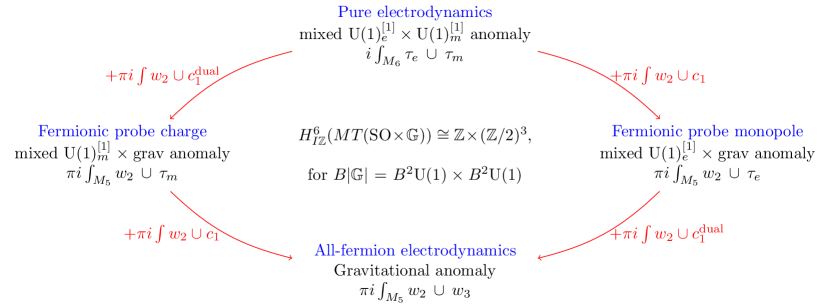
Figure 1: A map of the four possible ’t Hooft anomalies that can afflict a 4d theory with a pair of $\text{U}(1)$ 1-form global symmetries, defined on orientable manifolds without a spin structure. Each ’t Hooft anomaly corresponds to a factor in the cobordism group $H_{I\mathbb{Z}}^{6}\cong\mathbb{Z}\times(\mathbb{Z}/2)^{3}$, and is exhibited by Maxwell theory on its own (top, corresponding to the local $\mathbb{Z}$-valued anomaly) or coupled to a particular TQFT (left, bottom, and right, corresponding to the trio of global $\mathbb{Z}/2$-valued anomalies). The red arrows illustrate the relations between these four theories. For the global anomalies, these versions of 4d electromagnetism can also be realised as the boundary theories for 5d SPT phases.

Bordism generator for the $w_{2}\cup\tau_{e}$ anomaly.

Of course, it is important to note that $\mathbb{C}P^{2}$ is not nullbordant in $\Omega_{4}^{\text{SO}}$, given the signature $\sigma=1$ is a 4d bordism invariant. Given we saw the anomaly explicitly on $\mathbb{C}P^{2}$, one cannot in fact realise it via the counterterm $S_{\text{ct.}}=-\pi\text{i}\int_{X}w_{2}\cup\tau_{e}$ because there is no 5-manifold $X$ bounded by $M_{4}$. But as is well-known Freed:2004yc , the phase of the partition function $Z$ on such a non-nullbordant manifold suffers from an ambiguity, since it can always be shifted by a choice of generalized theta angle, i.e. a coupling to a non-trivial TQFT corresponding to an element in $\operatorname*{Hom}(\Omega_{4}^{\text{SO}}(\cdot),\mathbb{R}/\mathbb{Z})$. Thus, one can fix $\arg Z[M_{4},B_{e}]=\theta_{0}$ to a reference phase, and then $\arg Z$ is uniquely defined on any other 4-manifold $(M_{4}^{\prime},B_{e}^{\prime})$ that is bordant to $(M_{4},B_{e})$.

This phase can be calculated by constructing a 5d mapping torus $\tilde{X}$ by taking a cylinder that interpolates between $(M_{4},B_{e})$ and $(M_{4}^{\prime},B_{e}^{\prime})$, and gluing its ends to make a closed 5-manifold. This $\tilde{X}$ will be a representative of the generator of the $\mathbb{Z}/2$ factor in $\Omega_{5}^{\text{SO}}((B^{2}\text{U}(1))^{2})$ that we have claimed is dual to $w_{2}\cup\tau_{e}$.

In more detail, take $M_{4}=\mathbb{C}P^{2}$ and let $B_{e}^{0}$ denote any reference choice of background 2-form gauge field for the electric 1-form symmetry on $M_{4}$. Next take the product manifold $\mathbb{C}P^{2}\times[0,2\pi]$ with a product metric. Over the interval $I=[0,2\pi]$ one implements (for example linearly) the ‘large’ 2-form gauge transformation $B_{e}\mapsto B_{e}^{\prime}:=B_{e}+n\omega$, $n\in\mathbb{Z}$. Since $B_{e}$ and $B_{e}^{\prime}$ are gauge-equivalent, the manifold $\mathbb{C}P^{2}\times[0,2\pi]$ can be glued at 0 and $2\pi$ to make a closed 5-manifold with $\text{U}(1)$-2-bundle:

$$\tilde{X}:=S^{1}\times\mathbb{C}P^{2},\qquad B_{e}(\theta,z_{i})=B_{e}^{0}+\frac{t}{2\pi}n\omega,$$ (4.10)

where $t\in I$.

To verify that this mapping torus can be taken as a generator of the bordism group $\Omega^{\text{SO}}_{5}\left((B^{2}\text{U}(1))^{2}\right)$, it is enough to evaluate the bordism invariant ‘anomaly theory’ $w_{2}\cup\tau_{e}$ on $[\tilde{X}]$ and find a non-trivial value for the phase. Physically, evaluating $\langle w_{2}\cup\tau_{e},[\tilde{X}]\rangle$ computes the phase accrued by the partition function on $(\Sigma,B_{e})$ upon undergoing the 2-form gauge transformation $B_{e}\to B_{e}^{\prime}$. Doing the computation, we have that $\tau_{e}=\left[\frac{\text{d}t}{2\pi}\right]\cup\left[n\omega\right]=y\cup nx\in H^{3}(\tilde{X};\mathbb{Z}/2)$, where $x$ is the non-trivial element of $H^{2}(\tilde{X};\mathbb{Z}/2)$ obtained by pulling back $a$ along the projection $\tilde{X}\to\mathbb{C}P^{2}$, and $y$ is the non-trivial element of $H^{2}(\tilde{X};\mathbb{Z}/2)$ obtained by pulling back the generator of $H^{1}(S^{1};\mathbb{Z}/2)$ along $\tilde{X}\to S^{1}$. For $n$ odd, we have that $\tau_{e}=y\cup x$, the unique non-trivial element of $H^{3}(\tilde{X};\mathbb{Z}/2)$. Thus $w_{2}\cup\tau_{e}=x^{2}y\in H^{5}(\tilde{X};\mathbb{Z}/2)$ for $n$ odd, and so the anomaly theory evaluates to $1\text{~{}mod~{}}2$ on this mapping torus, while it is trivial for $n$ even.

The $w_{2}\cup\tau_{m}$ phase

An identical account can be given for the magnetic 1-form symmetry, if one replaces the topological coupling $\pi\text{i}\int w_{2}\cup c_{1}$ in (4.7) by $\pi\text{i}\int w_{2}\cup c_{1}^{\text{dual}}$, where $c_{1}^{\text{dual}}$ denotes the first Chern class of the electromagnetic dual of the gauge field. In that case, the 4d theory suffers from a ’t Hooft anomaly afflicting the magnetic 1-form symmetry, which obstructs $\text{U}(1)_{m}[1]$ from being gauged on non-spin manifolds such as $\mathbb{C}P^{2}$. The 5d anomaly theory is $\int_{M_{5}}w_{2}\cup\tau_{m}$.

Physically, this same anomaly can be understood from a different perspective. Suppose one couples vanilla Maxwell theory (4.1) to a charge-1 fermion, defined on all orientable 4-manifolds using a $\text{Spin}_{c}$ structure. The electric 1-form symmetry is explicitly broken, but one can still probe anomalies involving the magnetic 1-form symmetry and the gravitational background. The magnetic 1-form symmetry remains intact, even though we effectively have a ‘charge-$\frac{1}{2}$’ monopole due to the constraint $c_{1}=\frac{w_{2}\text{~{}mod~{}}2}{2}$ that follows the definition of $\text{Spin}_{c}$, because this monopole is not dynamical but rather acts as a constraint on the field configurations that are summed in the path integral. The symmetry type is now $\text{Spin}_{c}\times\mathbb{G}_{m}$, with $B|\mathbb{G}_{m}|=B^{2}\text{U}(1)_{m}$, for which the cobordism group $H_{I\mathbb{Z}}^{6}(MT(\text{Spin}_{c}\times\mathbb{G}_{m}))\cong\mathbb{Z}/2\times\mathbb{Z}^{2}$. Of course, all the anomalies involving the electric 1-form symmetry are absent, as is the $w_{2}w_{3}$ anomaly because the $\text{Spin}_{c}$ requirement trivialises $w_{3}$, but the $w_{2}\cup\tau_{m}$ global anomaly remains.

The $w_{2}\cup w_{3}$ phase

The final $\mathbb{Z}/2$-valued global anomaly that is detected by (4.6) corresponds to the 5d SPT phase $\int_{M_{5}}w_{2}\cup w_{3}$. To exhibit this anomaly, one starts from vanilla Maxwell theory and couples $w_{2}(TM_{4})$ as a background gauge field to both the electric and magnetic $\text{U}(1)$ 1-form symmetries. This SPT phase is purely gravitational and has been extensively analysed in the literature. Its boundary states include the theory of all-fermion electrodynamics Kravec:2014aza ; Wang:2018qoy and a fermionic theory with an emergent $\text{SU}(2)$ gauge symmetry Wang:2018qoy .

4.3 Scalar QED and 1-form anomaly interplay

Now let us couple Maxwell theory, defined as before with an SO structure, to a charge-2 boson. This coupling to matter breaks the electric 1-form symmetry down to a discrete remnant,

$$\text{U}(1)_{e}[1]\rightarrow\mathbb{Z}/2_{e}[1]\,,$$ (4.11)

while the full $\text{U}(1)_{m}[1]$ magnetic 1-form symmetry is preserved. This version of scalar QED therefore furnishes us with two global 1-form symmetries, one discrete and one continuous, and no 0-form symmetries. The classifying space of the global symmetry $\mathbb{G}^{\prime}$ is therefore

$$B|\mathbb{G}^{\prime}|=B^{2}\mathbb{Z}/2_{e}\times B^{2}\text{U}(1)_{m}\,,$$ (4.12)

and the 5d invertible field theories with this symmetry type are classified by the sequence (4.4) but with $|\mathbb{G}|$ replaced by $|\mathbb{G}^{\prime}|$. In Appendix B.2 we compute the relevant bordism groups to stitch together this generalized cohomology group.

Local anomalies:

We compute from Appendix B.2 that

$$\operatorname*{Hom}\left(\Omega_{6}^{\text{SO}}(B^{2}\mathbb{Z}/2_{e}\times B^{2}\text{U}(1)_{m}),\mathbb{Z}\right)=0\,,$$ (4.13)

and so there are no local anomalies; clearly, the mixed local ’t Hooft anomaly ‘$dB_{e}\cup dB_{m}$’ can no longer be realised now that one of the 1-form symmetries is broken to a discrete group, because the associated 2-form gauge field now has zero curvature.

Global anomalies:

On the other hand, we find that $\Omega^{\text{SO}}_{5}\left(B^{2}\mathbb{Z}/2\times B^{2}\text{U}(1)\right)=(\mathbb{Z}/2)^{4}$. The group classifying global anomalies is now

$$\operatorname*{Hom}\left(\operatorname*{Tor}\Omega_{5}^{\text{SO}}(B^{2}\mathbb{Z}/2_{e}\times B^{2}\text{U}(1)_{m}),\mathbb{R}/\mathbb{Z}\right)\cong(\mathbb{Z}/2)^{4}\,,$$ (4.14)

and we notice that there is an extra factor of $\mathbb{Z}/2$ corresponding to an extra global anomaly. At the level of characteristic classes, we can represent these four global anomalies in terms of products of Stiefel–Whitney classes and cohomology classes of $H^{\bullet}(B^{2}\text{U}(1)\times B^{2}\mathbb{Z}/2;\mathbb{Z}/2)$ that are in degree-5. There are five of them in total:

$$w_{2}\cup w_{3},\quad w_{2}\cup\tau_{m},\quad w_{2}\cup\text{~{}Sq}^{1}u_{2},\quad u_{2}\cup\tau_{m},\quad\text{~{}Sq}^{2}\text{~{}Sq}^{1}u_{2},$$

where $u_{2}$ is the unique generator of $H^{2}(B^{2}\mathbb{Z}/2;\mathbb{Z}/2)$ (see Appendix A.1). However, once pulled back to an orientable 5-manifold $X$, Wu’s relation Wu1950 tells us that $\text{~{}Sq}^{2}\text{~{}Sq}^{1}u_{2}=w_{2}(TX)\cup\text{~{}Sq}^{1}u_{2}$, so it is not an independent bordism invariant, and we end up with four invariants, as expected from the bordism group computation.

The anomaly interplay

Given an appropriate map $\pi$ between two spectra $MTH$ and $MTH^{\prime}$, there is an induced pullback map between the corresponding cobordism theories, $\pi^{\ast}:H_{I\mathbb{Z}}^{d+2}\left(MTH^{\prime}\right)\to H_{I\mathbb{Z}}^{d+2}\left(MTH\right)$, that can be used to relate anomalies between the two theories. This idea of ‘anomaly interplay’ has recently been used, for example, to relate local anomalies in 4d $\text{U}(2)$ gauge theory to Witten’s $\text{SU}(2)$ anomaly Davighi:2020bvi , to study anomalies in $\mathbb{Z}/k$ symmetries in 2d Grigoletto:2021zyv ; Grigoletto:2021oho with applications to bootstrapping conformal field theories, and to derive anomalies in non-abelian finite group symmetries in 4d Davighi:2022icj . Physically, the idea of ‘pulling back anomalies’ from one symmetry to another is not new, but goes back to Elitzur and Nair’s analysis of global anomalies Elitzur:1984kr , following Witten WITTEN1983422 . In all these cases the symmetry type takes the form $\{\text{Spin}\text{~{}or~{}}\text{SO}\}\times G^{[0]}$, where $G^{[0]}$ is a 0-form symmetry. In that case, a map of spectra $\pi$ is induced by any group homomorphism $\pi:G\to G^{\prime}$.

In the present case, where we have theories with 1-form global symmetries, it is straightforward to adapt this notion of anomaly interplay (which is just pullback in cobordism). Again, the crucial fact we use is that the nerves associated with the 1-form symmetries are themselves just ordinary (topological) groups, between which we can define group homomorphisms. Letting $\pi:\mathbb{Z}/2\to\text{U}(1):(1,-1)\to(1,e^{\text{i}\pi})$ denote the subgroup embedding, there is an associated map between symmetry types, $\pi:\text{SO}\times|\mathbb{G}^{\prime}|\to\text{SO}\times|\mathbb{G}|$ and an induced pullback map between the cobordism theories,

$$\pi^{\ast}:H_{I\mathbb{Z}}^{6}(MT(\text{SO}\times|\mathbb{G}^{\prime}|))\longrightarrow H_{I\mathbb{Z}}^{6}(MT(\text{SO}\times|\mathbb{G}|))\,.$$ (4.15)

Note that, since $H_{I\mathbb{Z}}^{\bullet}$ is a contravariant functor, the map between anomaly theories goes in the opposite direction to the subgroup embedding that we started with. Moreover, there is a pullback diagram for the whole short exact sequence characterizing $H_{I\mathbb{Z}}^{6}$, which encodes the notion of ‘anomaly interplay’:

$$\setcounter{MaxMatrixCols}{11}\begin{CD}0@>{}>{}>(\mathbb{Z}/2)^{4}@>{}>{}>(\mathbb{Z}/2)^{4}@>{}>{}>0@>{}>{}>0\\ @A{}A{}A@A{\pi^{\ast}}A{}A@A{}A{}A\\ 0@>{}>{}>(\mathbb{Z}/2)^{3}@>{}>{}>(\mathbb{Z}/2)^{3}\times\mathbb{Z}@>{}>{}>\mathbb{Z}@>{}>{}>0\,.\end{CD}$$ (4.16)

This anomaly interplay diagram can be used to track ’t Hooft anomalies in the 1-form global symmetries, through the ‘integrating in’ of a charge-2 boson.

Since all the generators of the cobordism groups can be represented by characteristic classes, we can represent the pullback $\pi^{\ast}$ by its action on the characteristic classes. The non-trivial action of $\pi^{\ast}$ is encoded in

$$\pi^{\ast}:\, \tau_{e}\cup\tau_{m}\mapsto u_{2}\cup\tau_{m},$$ (4.17)

$$w_{2}\cup\tau_{e}\mapsto w_{2}\cup\text{~{}Sq}^{1}u_{2}.$$ (4.18)

Trivially, $\pi^{\ast}$ maps $w_{2}\cup\tau_{m}$ and $w_{2}\cup w_{3}$ to themselves.

The most interesting pullback relation is Eq. (4.17), which says that a $\mathbb{Z}$-valued local anomaly pulls back to a $\mathbb{Z}/2$-valued global anomaly. This is somewhat analogous to the interplay studied in Davighi:2020bvi ; Davighi:2020uab between $\text{U}(2)$ local anomalies and $\text{SU}(2)$ global anomalies for 4d 0-form symmetries, where the maps there corresponded to pulling back exponentiated $\eta$-invariants.

To see how the interplay works in this example involving 1-form symmetries, which is arguably simpler than the story for chiral fermion anomalies, we follow the general methodology set out in Ref. Davighi:2020uab . To wit, we start with a 5-manifold $M_{5}$ representative of a class in $\Omega_{5}^{\text{SO}}(B^{2}\mathbb{Z}/2_{e}\times B^{2}\text{U}(1)_{m})$ that is dual to $u_{2}\tau_{m}$ (i.e. on which $u_{2}\tau_{m}$ evaluates to 1 mod 2). We choose

$$M_{5}=S^{2}_{e}\times S^{2}_{m}\times S^{1}_{\theta},$$ (4.19)

equipped with a $\mathbb{Z}/2$ background 2-bundle that has support only on $S^{2}_{e}$, and a $\text{U}(1)_{m}$ background 2-bundle that has support only on $S^{2}_{m}\times S^{1}_{\theta}$. Specifically, the $\mathbb{Z}/2$ 2-form connection has non-trivial 2-holonomy round $S_{e}^{2}$, viz $\int_{S^{2}_{e}}u_{2}=$ 1 mod 2. The $\text{U}(1)_{m}$ 2-form connection $B_{m}$ on $S^{2}_{m}\times S^{1}_{\theta}$ can be written $B_{m}=B_{m}^{0}+\frac{\theta}{2\pi}k\omega_{m}$, $k\in\mathbb{Z}$, where $\omega_{m}$ is the volume form on $S^{2}_{m}$ such that $\int_{S^{2}_{m}}\omega_{m}=1$, $B_{m}^{0}$ is any connection on the $S^{2}_{m}$ factor, and $\theta\in[0,2\pi)$ parametrizes $S^{1}_{\theta}$. The important thing is the flux relation

$$\int_{S^{2}_{m}\times S^{1}_{\theta}}dB_{m}=k\int_{S^{1}_{\theta}}\frac{d\theta}{2\pi}\int_{S^{2}_{m}}\omega_{m}=k\,.$$ (4.20)

Recalling $\tau_{m}=[dB_{m}/2\pi]_{\mathbb{Z}}$, integrating gives $\langle x_{2}\cup\tau_{m},[M_{5}]\rangle=k$ mod 2. When $k$ is odd, $M_{5}$ is not nullbordant, and the background fields cannot be simultaneously extended to any 6-manifold that $M_{5}$ bounds.

Now, to show that this global anomaly is the pullback under $\pi^{\ast}$ of the local anomaly $\tau_{e}\cup\tau_{m}$, we simply use the subgroup embedding $\pi:\mathbb{Z}/2\to\text{U}(1)$ to embed the $\mathbb{Z}/2$ 2-connection in an $\text{U}(1)$ 2-connection $B_{e}$. One can take

$$B_{e}=\frac{n}{2}\omega_{e},\qquad n\in 2\mathbb{Z}+1,\qquad\int_{S^{2}_{e}}\omega_{e}=1.$$ (4.21)

The 5-manifold (4.19) equipped with these structures $B_{e}$ and $B_{m}$ can be regarded as the pushforward in bordism of the $M_{5}$ that we started with, $\pi_{\ast}M_{5}$. This is nullbordant in $\Omega_{5}^{\text{SO}}(B^{2}\text{U}(1)_{e}\times B^{2}\text{U}(1)_{m})$; it can be realised as the boundary of a six-manifold $M_{6}=D^{3}_{e}\times S^{2}_{m}\times S^{1}_{\theta}$, where $D^{3}_{e}$ is one half of a 3-sphere $S^{3}$ that is bounded by $S^{2}_{e}$, to which the electric 2-form connection (4.21) can now be extended with $\int_{S^{3}}\frac{dB_{e}}{2\pi}=2n$. Using Stokes’ theorem, we thus have

$$\int_{S^{2}_{e}\times S^{2}_{m}\times S^{1}_{\theta}}\frac{B_{e}}{2\pi}\wedge\frac{dB_{m}}{2\pi}=\int_{D^{3}_{e}}\frac{dB_{e}}{2\pi}\int_{S^{2}_{m}\times S^{1}_{\theta}}\frac{dB_{m}}{2\pi}=nk\,,$$ (4.22)

obtaining the same phase from $\tau_{e}\tau_{m}$ as we did from $u_{2}\tau_{m}$.

On the other hand, we only need to see that the characteristic class $\tau_{e}$ reduces to the class $\text{~{}Sq}^{1}u_{2}$ when we restrict to a flat 2-bundle with mod 2 2-holonomy, in order to show that $w_{2}\cup\tau_{e}$ pulls back to $w_{2}\cup\text{~{}Sq}^{1}u_{2}$. To see this most clearly, it is best to use the language of cochains instead of differential forms. By identifying $\text{U}(1)$ with $\mathbb{R}/\mathbb{Z}$, we represent the $\text{U}(1)$ 2-form gauge field $B_{e}$ by a real 2-cochain $b_{e}$. If the gauge field is flat, $\delta b_{e}$ must be trivial as a cochain valued in $\mathbb{R}/\mathbb{Z}$. In other words, $\delta b_{e}$ is an integral 3-cochain, whose cohomology class can be identified with $\tau_{e}$. To use this flat $\text{U}(1)$ 2-cochain to describe a $\mathbb{Z}/2$ 2-form gauge field, we further impose that it must have mod 2 2-holonomy, i.e. $b_{e}$ must be half-integral-valued, not just any real cochain. Then $\tilde{b}_{e}:=2b_{e}$ is an integral cochain whose mod 2 reduction defines a cohomology class in $H^{2}(M_{5};\mathbb{Z}/2)$ that coincides with $u_{2}$. As $\text{~{}Sq}^{1}u_{2}=\beta_{2}(u_{2})$, where $\beta_{2}$ is the Bockstein homomorphism in the long exact sequence for cohomology

$$\ldots\rightarrow H^{n}(M_{5};\mathbb{Z}/2)\rightarrow H^{n}(M_{5};\mathbb{Z}/4)\rightarrow H^{n}(M_{5};\mathbb{Z}/2)\xrightarrow{\beta_{2}}H^{n+1}(M_{5};\mathbb{Z}/2)\rightarrow\ldots$$

induced by the short exact sequence $0\rightarrow\mathbb{Z}/2\rightarrow\mathbb{Z}/4\rightarrow\mathbb{Z}/2\rightarrow 0$, it can be represented by the mod 2 reduction of $\frac{1}{2}\delta\tilde{b}_{e}$. But this is exactly the same as $\delta b_{e}$ which represents $\tau_{e}$. Therefore, the mod 2 reduction of $\tau_{e}$ is $\text{~{}Sq}^{1}u_{2}$ when we embed the $\mathbb{Z}/2$ 1-form symmetry inside the $\text{U}(1)$ 1-form symmetry.

There will be no further examples of anomaly interplay in the present paper; in particular, we do not consider any examples with non-trivially fibred 2-groups (although see footnote 28 for some comments along these lines).

5 QED anomalies revisited

The Maxwell examples in the previous Section exhibited only 1-form global symmetries. In this Section, we move on to theories with both 0-form and 1-form global symmetries that are fused together in a non-trivial 2-group structure.

Quantum electrodynamics (QED) in 4d with certain fermion content furnishes us with such a theory. Here both the 0-form and 1-form symmetry groups are $\text{U}(1)$, and the 2-group structure is non-trivial when there is a mixed ’t Hooft anomaly between the global and gauged 0-form $\text{U}(1)$ currents, as was discovered in Cordova:2018cvg . There is a further possible ’t Hooft anomaly in the 2-group structure that comes from the usual cubic $\text{U}(1)$ anomaly for the 0-form symmetry, but, rather than being a $\mathbb{Z}$-valued local anomaly, the 2-group structure transmutes this cubic anomaly to a discrete, $\mathbb{Z}/m$-valued global anomaly Cordova:2018cvg , with $m$ given by the modulus of the integral Postnikov class of the 2-group. After reviewing the physics arguments for these statements, we derive them from the cobordism perspective. Our spectral sequence calculations reproduce the order of the finite $\mathbb{Z}/m$ anomaly.

5.1 From the physics perspective

Consider a system of Weyl fermions coupled to a $\text{U}(1)_{a}$ gauge group with dynamical gauge field $a$. Assuming that a fermion with unit charge is present, the electric 1-form symmetry is broken completely. This leaves only the magnetic $\text{U}(1)^{[1]}$ 1-form symmetry, with 2-form current $j^{m}=\star\frac{f}{2\pi}$ as in (4.2), where $f=\text{d}a$. Given enough Weyl fermions, one can find a global $\text{U}(1)^{[0]}$ 0-form symmetry that does not suffer from the ABJ anomaly. It is possible, however, that upon coupling a background gauge field $A$ to this global 0-form symmetry, there is an operator-valued mixed anomaly that is captured by the anomaly polynomial term

$$\Phi_{6}\supset\frac{\kappa}{16\pi^{3}}f\wedge F\wedge F\,,$$ (5.1)

where $F=dA$ is the field strength for the background gauge field $A$. It describes, via the usual descent procedure, the shift in the effective action under the background gauge transformation $A\mapsto A+\text{d}\lambda^{(0)}$, with $\lambda^{(0)}$ a $2\pi$-periodic scalar, by

$$\delta S=\frac{\text{i}\kappa}{2}\int_{M_{4}}\lambda^{(0)}\frac{f\wedge F}{4\pi^{2}}\,.$$ (5.2)

It was realised in Ref. Cordova:2018cvg that we should not interpret this term as an anomaly, but rather as a non-trivial 2-group structure.

To see why this is the case, we first couple a 2-form background gauge field $B^{(2)}$, which satisfies the usual normalisation condition

$$\int_{M_{3}}\frac{\text{d}B^{(2)}}{2\pi}\in\mathbb{Z}$$ (5.3)

on closed 3-manifolds, to the magnetic 1-form symmetry via the coupling

$$S_{\text{coupling}}=\frac{\text{i}}{2\pi}\int_{M_{4}}f\wedge B^{(2)}.$$ (5.4)

Then the potential anomaly (5.2) can be cancelled by modifying the background gauge transformation for $B^{(2)}$ from an ordinary 1-form gauge transformation $B^{(2)}\mapsto B^{(2)}+\text{d}\lambda^{(1)}$, that is independent of the 0-form gauge transformation of $A$, to a 2-group gauge transformation

$$A\mapsto A+\text{d}\lambda^{(0)},\qquad B^{(2)}\mapsto B^{(2)}+\text{d}\lambda^{(1)}+\frac{\hat{\kappa}}{2\pi}\lambda^{(0)}F,$$ (5.5)

provided that we identify $\hat{\kappa}$ with $-\kappa/2$. Here the gauge transformation parameter $\lambda^{(1)}$ is a properly normalised $\text{U}(1)$ gauge field.

This modified transformation mixes the magnetic $\text{U}(1)^{[1]}$ 1-form symmetry with the $\text{U}(1)^{[0]}$ 0-form symmetry, and encodes the 2-group structure at the level of the background fields. In our quadruplet notation, the 2-group is

$$\mathbb{G}=(\text{U}(1),\text{U}(1),0,\hat{\kappa}),$$ (5.6)

with the Postnikov class $\hat{\kappa}\in H^{3}(B\text{U}(1);\text{U}(1))\cong\mathbb{Z}$, where we use the fact that $H^{3}(B\text{U}(1);\text{U}(1))$ with continuous $\text{U}(1)$ coefficients is isomorphic to $H^{4}(B\text{U}(1);\mathbb{Z})\cong\mathbb{Z}$ via the universal coefficient theorem. The nerve of such a 2-group is the extension

$$|\mathbb{G}|=\text{U}(1)^{[0]}\times_{\hat{\kappa}}\text{U}(1)^{[1]}.$$ (5.7)

The non-trivial 2-group structure can also be seen without turning on the background gauge fields explicitly. If we write $j$ for the 1-form current associated with $\text{U}(1)^{[0]}$, then the Ward identity takes the non-trivial form

$$\partial^{\mu}j_{\mu}(x)j_{\nu}(y)=\frac{\hat{\kappa}}{2\pi}\partial^{\lambda}\delta^{(4)}(x-y)j^{m}_{\nu\lambda}(y)\,,$$ (5.8)

where $j^{m}_{\nu\lambda}$ are the components of the magnetic 2-form current $j^{m}$. This Ward identity shows how the 0-form and 1-form currents are fused, realising Eq. (1.3).

The 2-group symmetry $\text{U}(1)^{[0]}\times_{\hat{\kappa}}\text{U}(1)^{[1]}$ can still suffer from an ’t Hooft anomaly. Recall that, when $\hat{\kappa}=0$, the anomaly polynomial for our system of Weyl fermions is

$$\Phi_{6}=\frac{\mathcal{A}_{3}}{6}c_{1}(F)^{3}-\frac{\mathcal{A}_{\text{mixed}}}{24}p_{1}(R)c_{1}(F),$$ (5.9)

where $c_{1}(F)=F/2\pi$ is the first Chern class of the $\text{U}(1)^{[0]}$ bundle, and $p_{1}(R)=\frac{1}{8\pi^{2}}\text{Tr}\,R\wedge R$ is the first Pontryagin class of the tangent bundle, where $R$ is the curvature 2-form. Before we continue, it is important to discuss the role of these anomaly coefficients in the (co)bordism context, still for the case $\hat{\kappa}=0$. Naïvely, one might think that the cubic anomaly coefficient $\mathcal{A}_{3}$ and the mixed $\text{U}(1)$-gravitational anomaly coefficient $\mathcal{A}_{\text{mixed}}$ are the two integers that classify anomalies according to cobordism, i.e. that $\mathcal{A}_{3}$ and $\mathcal{A}_{\text{mixed}}$ can be chosen as generators of the group $\operatorname*{Hom}\left(\Omega^{\text{Spin}}_{6}\left(B\text{U}(1)\right),\mathbb{Z}\right)\cong\mathbb{Z}\times\mathbb{Z}$. However, this is not the correct identification because $\mathcal{A}_{3}$ and $\mathcal{A}_{\text{mixed}}$ are not quite independent. It can be shown that

$$\alpha_{1}:=c_{1}(F)^{3}\qquad\text{and}\qquad\alpha_{2}:=\frac{c_{1}(F)}{6}\left(c_{1}(F)^{2}-\frac{1}{4}p_{1}(R)\right)$$ (5.10)

are independent integral cohomology classes. In terms of these basis generators, we can write $\Phi_{6}$ as

$$\Phi_{6}=\frac{1}{6}\left(\mathcal{A}_{3}-\mathcal{A}_{\text{mixed}}\right)\alpha_{1}+\mathcal{A}_{\text{mixed}}\alpha_{2}.$$ (5.11)

Again, by the Atiyah–Singer index theorem, $\Phi_{6}$ must be integral. Since $\alpha_{1}$ and $\alpha_{2}$ are integral basis generators, we can deduce that the two integers $(r,s)$ that label $\operatorname*{Hom}\left(\Omega^{\text{Spin}}_{6}\left(B\text{U}(1)\right),\mathbb{Z}\right)$ are

$$(r,s)=\left(\frac{1}{6}\left(\mathcal{A}_{3}-\mathcal{A}_{\text{mixed}}\right),\mathcal{A}_{\text{mixed}}\right).$$ (5.12)

Continuing, let’s switch the Postnikov class $\hat{\kappa}$ back on, and couple the background 2-form gauge field $B^{(2)}$ to the $\text{U}(1)^{[1]}$ 1-form symmetry. We are free to add a Green–Schwarz counter-term

$$S_{\text{GS}}=\frac{in}{2\pi}\int_{M_{4}}B^{(2)}\wedge F,\qquad n\in\mathbb{Z}$$ (5.13)

to the action. Under the 2-group transformation (5.5), the effective action shifts if the anomaly coefficients $\mathcal{A}_{3}$ and $\mathcal{A}_{\text{mixed}}$ are non-zero, by

$$\delta S=\text{i}\frac{\mathcal{A}_{3}+6n\hat{\kappa}}{6}\int_{M_{4}}\lambda^{(0)}\frac{F\wedge F}{4\pi^{2}}-\text{i}\frac{\mathcal{A}_{\text{mixed}}}{24}\int_{M_{4}}\lambda^{(0)}p_{1}(R).$$ (5.14)

Since one may choose the counterterm coefficient $n$ to be any integer, one sees that $\mathcal{A}_{3}$ is only well-defined modulo $6\hat{\kappa}$ Cordova:2018cvg . It follows that the integer $r=\frac{1}{6}\left(\mathcal{A}_{3}-\mathcal{A}_{\text{mixed}}\right)$ that we claim classifies the anomaly is not really valued in $\mathbb{Z}$, being well-defined only modulo $|\hat{\kappa}|$. This corresponds to a global anomaly in the 2-group symmetry, that is valued in the cyclic group

$$\mathbb{Z}/m,\qquad m=|\hat{\kappa}|.$$ (5.15)

We emphasize that, even though $\mathcal{A}_{3}$ is well-defined modulo $6\hat{\kappa}$ (as was derived in Cordova:2018cvg ), the discrete group that classifies the global anomaly has order $|\hat{\kappa}|$ (and not $6|\hat{\kappa}|$). The mixed gravitational anomaly remains a $\mathbb{Z}$-valued local anomaly.

5.2 From the bordism perspective

In this Section we show how the ’t Hooft anomalies afflicting the 2-group global symmetry, that we have just described, can be precisely understood using cobordism. To do so, we need to compute the generalized cohomology groups

$$H^{6}_{I\mathbb{Z}}\left(MT\left(\text{Spin}\times|\mathbb{G}|\right)\right),\qquad|\mathbb{G}|=U(1)^{[0]}\times_{\hat{\kappa}}U(1)^{[1]}\,,$$ (5.16)

which are built from $\Omega_{5}^{\text{Spin}}(B|\mathbb{G}|)$ and $\Omega_{6}^{\text{Spin}}(B|\mathbb{G}|)$, for each value of the Postnikov class $\hat{\kappa}$. These abelian groups detect and classify all possible anomalies for this 2-group symmetry type.

To compute these bordism groups, we follow the general strategy outlined in §3.2. We first apply the cohomological Serre spectral sequence to the fibration

$$K(\mathbb{Z},3)\to B|\mathbb{G}|\to K(\mathbb{Z},2)$$ (5.17)

to calculate the cohomology of $B|\mathbb{G}|$ in relevant low degrees. Then we will convert the result into homology groups, which are fed into the Atiyah–Hirzebruch spectral sequence for the fibration $\text{pt}\to B|\mathbb{G}|\to B|\mathbb{G}|$, for which the second page is $E^{2}_{p,q}=H_{p}\left(B|\mathbb{G}|;\Omega^{\text{Spin}}_{q}(\text{pt})\right)$, to compute the spin bordism.

So, to begin, the $E_{2}$ page of the cohomological Serre spectral sequence for the fibration (5.17) is given by

$$E_{2}^{p,q}=H^{p}\big{(}K(\mathbb{Z},2);H^{q}(K(\mathbb{Z},3);\mathbb{Z})\big{)}.$$ (5.18)

Using $H^{\bullet}(K(\mathbb{Z},3);\mathbb{Z})\cong\{\mathbb{Z},0,0,\mathbb{Z},0,0,\mathbb{Z}/2,0,\mathbb{Z}/3,\mathbb{Z}/2,\ldots\}$, given in Table 3 of Appendix A.1, we can construct the $E_{2}$ page as shown in the left-hand side of Fig. 2. In fact, what is shown there is the $E_{4}$ page, since the entries are sparse enough that there are no non-trivial differentials in the region we are interested in until page $E_{4}$.

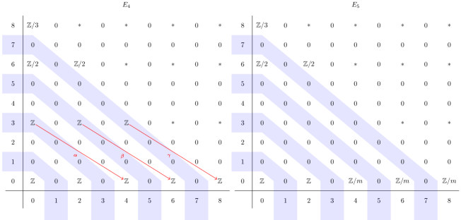
Figure 2: Fourth and fifth pages of the Serre spectral sequence to compute the integral cohomology of the fibration $K(\mathbb{Z},3)\to B|\mathbb{G}|\to K(\mathbb{Z},2)$.

The differentials $\alpha$, $\beta$, and $\gamma$ shown on the left-hand diagram of Fig. 2 are linear in the Postnikov class $\hat{\kappa}\in\mathbb{Z}$ (see the Appendix of Ref. Kapustin:2013uxa ). More precisely, we write

$$H^{3}(K(\mathbb{Z},3);\mathbb{Z})\cong\operatorname*{Hom}(\mathbb{Z}^{[1]},\mathbb{Z})\cong\mathbb{Z}$$

using the universal coefficient theorem and the fact that $K(\mathbb{Z},3)=B^{2}\text{U}(1)^{[1]}=B^{3}\mathbb{Z}^{[1]}$. Here, we include the superscript to emphasise that this $\mathbb{Z}$ comes from our $\text{U}(1)$ 1-form symmetry part. From this, we can write the entry $E^{0,3}_{4}$ in the Serre spectral sequence as $\operatorname*{Hom}(\mathbb{Z}^{[1]},\mathbb{Z})$. Then, the differential $\alpha$ is given by ‘contraction’ (adopting the terminology of Kapustin:2013uxa ) with the Postnikov class

$$\begin{split}\alpha:\operatorname*{Hom}(\mathbb{Z}^{[1]},\mathbb{Z})&\to H^{4}(B\text{U}(1)^{[0]};\mathbb{Z})\\ x&\mapsto x\circ\hat{\kappa}\end{split}$$ (5.19)

where we make use of the fact that the Postnikov class is a cohomology class

$$\hat{\kappa}\in H^{3}(B\text{U}(1)^{[0]},\text{U}(1)^{[1]})\cong H^{4}(B\text{U}(1)^{[0]};\mathbb{Z}^{[1]})\;.$$

Similar arguments apply for the differentials $\beta$ and $\gamma$. Thus, $\alpha$, $\beta$, and $\gamma$ map $1$ to $\pm\hat{\kappa}$, resulting in the $E_{5}$ page as shown, where $m:=|\hat{\kappa}|$. We can then read off the integral cohomology groups to be

$$H^{\bullet}(B|\mathbb{G}|;\mathbb{Z})\cong\{\mathbb{Z},0,\mathbb{Z},0,\mathbb{Z}/m,0,e(\mathbb{Z}/2,\mathbb{Z}/m),0,e(\mathbb{Z}/6,\mathbb{Z}/m),\ldots\}\,$$ (5.20)

where the notation $e(A,B)$ denotes an extension of $A$ by $B$, viz. a group that fits in the short exact sequence $B\hookrightarrow e(A,B)\twoheadrightarrow A$. We compute the mod 2 cohomology by the same method in Appendix A.2.

Heuristically, one can also argue for the form of $\alpha$ and $\beta$ as follows (c.f. Appendix B.6 of Ref. Lee:2020ewl ). Let us start with a representative of a generator of the cohomology group $H^{3}(K(\mathbb{Z},3),\mathbb{Z})\cong\mathbb{Z}$, and ask what it becomes when $K(\mathbb{Z},3)$ is the fibre of $B|\mathbb{G}|$. Given the normalisation condition (5.3), the 3-form

$$\tilde{h}:=\text{d}B^{(2)}/2\pi$$ (5.21)

represents the generator of $H^{3}(K(\mathbb{Z},3);\mathbb{Z})\cong\mathbb{Z}$. This is true when $K(\mathbb{Z},3)$ stands on its own. However, when we pass to the 2-group $\mathbb{G}$ and take $K(\mathbb{Z},3)$ to be the fibre of $B|\mathbb{G}|$, then $\tilde{h}$ is not gauge-invariant under (5.5) for a general Postnikov class, and cannot be a representative of any cohomology class for $B|\mathbb{G}|$. We can remedy this by modifying the definition of $\tilde{h}$ to

$$h:=\tilde{h}-\frac{\hat{\kappa}}{2\pi}A\wedge F.$$ (5.22)

The trade off is that the gauge-invariant $h$ is no longer closed; instead

$$\text{d}h=-\frac{\hat{\kappa}}{4\pi^{2}}F\wedge F=-\hat{\kappa}c_{1}\cup c_{1},$$ (5.23)

where $c_{1}:=\frac{F}{2\pi}$ is the first Chern class of the $U(1)^{[0]}$ bundle, and $c_{1}\cup c_{1}$ can be taken as the generator of $H^{4}(K(\mathbb{Z},2);\mathbb{Z})$. The 2-group relation (5.23) implies that both the differentials $\alpha$ and $\beta$ in Fig. 2 map $1$ to $-\hat{\kappa}$.

From this cohomological starting point, we can proceed to compute the spin bordism groups. We find it is helpful to split the discussion into the cases where $m$ is even or odd, for which the bordism group calculations are tackled using different tricks. As a warm up, we first consider the simplest case where $m$ is zero, corresponding to a 0-form and 1-form symmetry that do not mix.

5.2.1 Zero Postnikov class

We first consider the trivial toric 2-group where $B|\mathbb{G}|$ is a simply a product space $K(\mathbb{Z},2)\times K(\mathbb{Z},3)$. As $B|\mathbb{G}|$ is a product, we can use the Künneth theorem to determine the homology groups of $K(\mathbb{Z},2)\times K(\mathbb{Z},3)$ from the homology groups of each factor, given by Eq. (A.2) and Table 3 in Appendix A.1. We obtain

$$H_{\bullet}(K(\mathbb{Z},2)\times K(\mathbb{Z},3);\mathbb{Z})\cong\left\{\mathbb{Z},0,\mathbb{Z},\mathbb{Z},\mathbb{Z},\mathbb{Z}\times\mathbb{Z}/2,\mathbb{Z},\mathbb{Z}\times\mathbb{Z}/6,\mathbb{Z}\times\mathbb{Z}/2,\ldots\right\}$$ (5.24)

and construct the second page of the AHSS as shown in Fig. 3, with non-trivial differentials on the $E^{2}$ page indicated by coloured arrows.

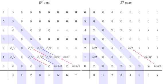
Figure 3: The $E^{2}$ and $E^{3}$ pages for the Atiyah–Hirzebruch spectral sequence for $\Omega^{\text{Spin}}_{\bullet}(K(\mathbb{Z},2)\times K(\mathbb{Z},3))$.

The differentials on the zeroth and the first rows are the composition $\widetilde{\text{Sq}^{2}}\circ\rho_{2}$ and $\widetilde{\text{Sq}^{2}}$, respectively, where $\rho_{2}$ is reduction modulo 2. To compute the action of these differentials, we need to know how the Steenrod squares act on the mod 2 cohomology ring of the product $K(\mathbb{Z},2)\times K(\mathbb{Z},3)$. From the mod 2 cohomology rings of $K(\mathbb{Z},2)$ and $K(\mathbb{Z},3)$ given by (A.3) and (A.4), we obtain

$$H^{\bullet}(K(\mathbb{Z},2)\times K(\mathbb{Z},3);\mathbb{Z}/2)\cong\mathbb{Z}/2[c_{1},\tau_{3},\text{~{}Sq}^{2}\tau_{3},\text{~{}Sq}^{4}\text{~{}Sq}^{2}\tau_{3},\ldots],$$ (5.25)

where $c_{1}$ and $\tau_{3}$ are the unique generators in degree $2$ and $3$, respectively. In our diagram, the red maps correspond to $\text{Sq}^{2}c_{1}=c_{1}^{2}$, the blue maps to $\text{Sq}^{2}\tau_{3}$ being a generator of $H^{\bullet}(K(\mathbb{Z},3);\mathbb{Z}/2)$, and the magenta maps to $\text{Sq}^{2}(c_{1}\tau_{3})=c_{1}^{2}\tau_{3}$. The differential depicted in the $E^{3}$ page from $E_{7,0}^{3}$ in the diagram must be non-trivial by comparing $\Omega^{\text{Spin}}_{6}(K(\mathbb{Z},2)\times K(\mathbb{Z},3))$ with the result computed with the Adams spectral sequence. We can then read off the bordism groups in lower degrees, which we collect below in Table 1. We piece together the cobordism group

$$H_{I\mathbb{Z}}^{6}(MT(\text{Spin}\times\text{U}(1)\times B\text{U}(1)))\cong\mathbb{Z}\times\mathbb{Z},$$ (5.26)

which classifies anomalies for this symmetry type. The pair of $\mathbb{Z}$-valued local anomalies anomalies just corrresponds to the usual cubic $c_{1}^{3}$ and mixed gravitational $c_{1}p_{1}$ anomalies associated with the $\text{U}(1)$ 0-form symmetry. The presence of the 1-form symmetry here plays no role in anomaly cancellation for this dimension.

5.2.2 Even Postnikov class

Now we turn to the case where $m=|\hat{\kappa}|$ is a non-zero even integer. Continuing from the cohomology calculation above, summarised in Eq. (5.20), there are two options for the extension $e(\mathbb{Z}/2,\mathbb{Z}/m)$; either the trivial extension $\mathbb{Z}/2\times\mathbb{Z}/m$ or the non-trivial one $e(\mathbb{Z}/2,\mathbb{Z}/m)\cong\mathbb{Z}/(2m)$, which are non-isomorphic. By comparing the mod 2 cohomology calculated from applying the universal coefficient theorem to (5.20) and the one calculated directly from the Serre spectral sequence, one can show that the correct extension is the direct product $\mathbb{Z}/2\times\mathbb{Z}/m$. The integral homology for $B|\mathbb{G}|$ is then

$$H_{\bullet}\left(B|\mathbb{G}|;\mathbb{Z}\right) \cong\left\{\mathbb{Z},0,\mathbb{Z},\mathbb{Z}/m,0,\mathbb{Z}/m\times\mathbb{Z}/2,0,e(\mathbb{Z}/6,\mathbb{Z}/m),\ldots\right\}$$ (5.27)

and the mod 2 homology is

$$H_{\bullet}(B|\mathbb{G}|;\mathbb{Z}/2)\cong\left\{\mathbb{Z}/2,0,\mathbb{Z}/2,\mathbb{Z}/2,\mathbb{Z}/2,\mathbb{Z}/2\times\mathbb{Z}/2,\ldots\right\}\,,$$ (5.28)

The $E^{2}$ page of the AHSS is then given by Fig. 4. We observe that there are non-vanishing differentials already on the $E^{2}$ page (which will not be the case when we turn to the case of odd $m$). These non-trivial $E^{2}$ differentials make the spectral sequence easier to compute, as follows.

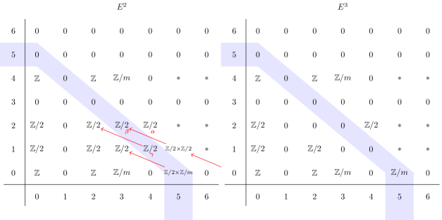
Figure 4: The $E^{2}$ page of the AHSS for the fibration $\text{pt}\to B|\mathbb{G}|\to B|\mathbb{G}|$ when $\mathbb{G}$ is the 2-group $\text{U}(1)^{[0]}\times_{\hat{\kappa}}\text{U}(1)^{[1]}$ with $m:=|\hat{\kappa}|$ even.

The differentials $\alpha$ and $\beta$ on the second page are duals $\widetilde{\text{~{}Sq}^{2}}$ of the Steenrod square $\text{~{}Sq}^{2}$, while the differential $\gamma$ is a mod 2 reduction followed by the dual of $\mathrm{Sq}^{2}$ teichner1993signature . The Steenrod square dual to $\beta$ sends a unique generator in $H^{2}(B|\mathbb{G}|;\mathbb{Z}/2)$ to a unique generator in $H^{4}(B|\mathbb{G}|;\mathbb{Z}/2)$ (c.f. Appendix A.2), so $\beta$ must be the non-trivial map from $\mathbb{Z}/2$ to $\mathbb{Z}/2$, killing off both factors. Similarly, the Steenrod square dual to $\alpha$ acts on the unique generator of $H^{3}(B|\mathbb{G}|;\mathbb{Z}/2)$ that comes from the generator $\tau_{3}\in H^{3}(K(\mathbb{Z},3);\mathbb{Z}/2)$ of the fibre, which we will also label by $\tau_{3}$. The image is a generator of $H^{5}(B|\mathbb{G}|;\mathbb{Z}/2)$ that comes from $\text{Sq}^{2}\tau_{3}$ of $H^{5}(K(\mathbb{Z},3);\mathbb{Z}/2)$. It generates the $\mathbb{Z}/2$ factor in the mod 2 cohomology that is a reduction from the $\mathbb{Z}/2$ factor in the integral cohomology, and not the $\mathbb{Z}/m$ factor since it is the $\mathbb{Z}/2$ factor that arise from the fibre’s contribution. Therefore, both $\alpha$ and $\gamma$ must be non-trivial, with $\ker\gamma\cong\mathbb{Z}/m$, as indicated in the $E^{3}$ page in Fig. 4.

Before continuing, we pause here to emphasize the importance of using (spin) cobordism, rather than just cohomology, to study ’t Hooft anomalies in these theories. At the level of cohomology, the existence of a non-trivial $\mathbb{Z}/2$-valued cohomology class $\text{Sq}^{2}\tau_{3}\in H^{5}(K(\mathbb{Z},3);\mathbb{Z}/2)$ might suggest there is a non-trivial SPT phase on 5-manifolds $M_{5}$, or equivalently a non-trivial anomaly theory for the corresponding 4d theory, with partition function

$$Z=\exp\left(\pi\text{i}\int_{M_{5}}\text{Sq}^{2}\tau_{3}\right),$$ (5.29)

where $\text{Sq}^{2}\tau_{3}$ is pulled back to $M_{5}$. But, one can use Wu’s relation to trade the Steenrod square operation for a Stiefel–Whitney class Wu1950 , viz.

$$Z=\exp\left(\pi\text{i}\int_{M_{5}}w_{2}(TM_{5})\cup\tau_{3}\right).$$ (5.30)

If we now restrict to $M_{5}$ being a spin manifold, then $w_{2}(TM_{5})$ is trivial and we immediately learn that this SPT phase is trivial. Of course, this ‘trivialisation’ of the SPT phase corresponding to the cohomology class in $H^{5}(K(\mathbb{Z},3);\mathbb{Z}/2)$ is automatically captured by the spectral sequence computation for spin bordism, by the non-triviality of the map $\gamma$ on turning from the second to the third page of the AHSS.

Continuing with the bordism computation, we now find that the entries in the range $p+q\leq 5$ stabilise on this $E^{3}$ page, whence we can read off the spin bordism groups for 2-group symmetry $\mathbb{G}=\text{U}(1)^{[0]}\times_{\hat{\kappa}}\text{U}(1)^{[1]}$ with even Postnikov class $\hat{\kappa}$ up to degree-5, which are listed in Table 1. There is still an undetermined group extension in $\Omega^{\text{Spin}}_{3}(B|\mathbb{G}|)$ but we will argue from the physics point of view in Section 6 that it must be the non-trivial extension $\mathbb{Z}/(2m)$. In summary, our results are those given in Table 1.

$i$	$0$	$1$	$2$	$3$	$4$	$5$	$6$
$\Omega^{\text{Spin}}_{i}(B|\mathbb{G}|)$, $\hat{\kappa}\neq 0$	$\mathbb{Z}$	$\mathbb{Z}/2$	$\mathbb{Z}\times\mathbb{Z}/2$	$\mathbb{Z}/(2|\hat{\kappa}|)$	$\mathbb{Z}$	$\mathbb{Z}/|\hat{\kappa}|$	$\mathbb{Z}\times\text{Tors}$
$\Omega^{\text{Spin}}_{i}(B|\mathbb{G}|)$, $\hat{\kappa}=0$	$\mathbb{Z}$	$\mathbb{Z}/2$	$\mathbb{Z}\times\mathbb{Z}/2$	$\mathbb{Z}$	$\mathbb{Z}\times\mathbb{Z}$	$\mathbb{Z}$	$\mathbb{Z}\times\mathbb{Z}\times\text{Tors}$

Table 1: Spin bordism groups for the twisted 2-group symmetry $\mathbb{G}=\text{U}(1)^{[0]}\times_{\hat{\kappa}}\text{U}(1)^{[1]}$. Here, Tors denotes an undetermined pure torsion part. For comparison, we also include the bordism groups in the case $\hat{\kappa}=0$, which corresponds to a direct product of 0-form and 1-form symmetries. One can thus see how, for both 2d and 4d quantum field theories, local anomalies in the untwisted case morph into global anomalies when the Postnikov class $\hat{\kappa}$ is turned on, thanks to a Green–Schwarz-like mechanism.

5.2.3 Odd Postnikov class

We now turn to the case where $m$ is odd, for which the spin bordism computation turns out to be rather more difficult, technically. Firstly, when $m$ is odd, the extension $e(\mathbb{Z}/2,\mathbb{Z}/m)$ is unambiguously $\mathbb{Z}/m\times\mathbb{Z}/2$ (which is, for odd $m$, isomorphic to $\mathbb{Z}/(2m)$). The integral homology of $B|\mathbb{G}|$ is as written in Eq. (5.27), and the mod 2 homology groups are now

$$H_{\bullet}\left(B|\mathbb{G}|;\mathbb{Z}/2\right) \cong\left\{\mathbb{Z}/2,0,\mathbb{Z}/2,0,0,\mathbb{Z}/2,\ldots\right\}$$ (5.31)

by the universal coefficient theorem. Now we feed these results into the AHSS for the trivial point fibration $\text{pt}\to B|\mathbb{G}|\to B|\mathbb{G}|$. The $E^{2}$ has no non-trivial differentials in the range of interest.

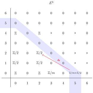
Figure 5: The $E^{3}$ page of the AHSS for the fibration $\text{pt}\to B|\mathbb{G}|\to B|\mathbb{G}|$ when $\mathbb{G}$ is the 2-group $\text{U}(1)^{[0]}\times_{\hat{\kappa}}\text{U}(1)^{[1]}$ with $m:=|\hat{\kappa}|$ odd.

The $E^{3}$ page is shown in Fig. 5, with a single potentially non-trivial differential in the range of interest, $\text{d}_{3}:E^{3}_{5,0}\to E^{3}_{2,2}$. If this differential were trivial, then $\Omega^{\text{Spin}}_{5}(B|\mathbb{G}|)$ would equal $\mathbb{Z}/m\times\mathbb{Z}/2$, and $\Omega^{\text{Spin}}_{4}(B|\mathbb{G}|)$ would equal $\mathbb{Z}\times\mathbb{Z}/2$. The factor of $\mathbb{Z}/m$ in $\Omega^{\text{Spin}}_{5}(B|\mathbb{G}|)$ would correspond to the global anomaly that we described in the previous Section, which we know to be valued in $\mathbb{Z}/m$ as in (5.15). The extra factor of $\mathbb{Z}/2$ would presumably correspond to a further global anomaly that we have not seen so far by physics arguments. On the other hand, if this differential were the non-trivial map, then $\Omega^{\text{Spin}}_{5}(B|\mathbb{G}|)$ would equal $\mathbb{Z}/m$, agreeing precisely with the physics account, and $\Omega^{\text{Spin}}_{4}(B|\mathbb{G}|)$ would just equal $\mathbb{Z}$.

It turns out that this all-important $d_{3}$ differential is non-trivial. But being a differential on the third page, there are no straightforwardly-applicable formulae (analogous to the formulae in terms of Steenrod squares that are available on the second page) that we can use to compute it directly. Indeed, our usual AHSS plus ASS techniques are not sufficient to constrain this differential. This differential can nonetheless be evaluated using different arguments, which we present in Appendix C. The gist of the argument is as follows.

The central character is a long exact sequence in bordism groups, analogous to the Gysin long exact sequence in ordinary homology, of the form

$$\dots\to\Omega^{\text{Spin}}_{d}(S(V))\to\Omega^{\text{Spin}}_{d}(B|\mathbb{G}|)\to\Omega^{\text{Spin}}_{d-2}((B|\mathbb{G}|)^{V-2})\to\Omega^{\text{Spin}}_{d}(S(V))\to\dots$$ (5.32)

Here $V\to B|\mathbb{G}|$ is the pullback bundle (which is rank 2) of the tautological line bundle $L\to B\text{U}(1)^{[0]}$ along the quotient map $q:B|\mathbb{G}|\to B\text{U}(1)^{[0]}$, $S(V)\to B|\mathbb{G}|$ is the associated sphere bundle of $V$, and $(B|\mathbb{G}|)^{V-2}$ is the Thom spectrum of the virtual bundle. This long exact sequence in bordism is extremely powerful: by proving that the groups $\Omega^{\text{Spin}}_{5}(S(V))$ and $\Omega^{\text{Spin}}_{3}((B|\mathbb{G}|)^{V-2})$ both lack free and 2-torsion summands, one learns that the group $\Omega^{\text{Spin}}_{5}(B|\mathbb{G}|)$ in the middle, which is our bordism group of interest, also lacks 2-torsion. The $\mathbb{Z}/2$ factor discussed above is therefore absent (from which we learn that it must be killed by the differential $d_{3}$ which is therefore non-trivial).

Putting things together, we can thus extract all the spin bordism groups for 2-group symmetry $\mathbb{G}=\text{U}(1)^{[0]}\times_{\hat{\kappa}}\text{U}(1)^{[1]}$, with odd Postnikov class $\hat{\kappa}$, up to degree-5.

5.2.4 The free part

When $m$ is non-trivial, regardless of its parity, we can also show that the free part of $\Omega^{\text{Spin}}_{6}(B|\mathbb{G}|)$ is given by $\mathbb{Z}$ coming from the entry $E^{r}_{2,4}$. First, observe that the free part of the $\Omega^{\text{Spin}}_{6}(B|\mathbb{G}|)$, if there is one at all, can only come from this entry as any other entry from the diagonal $p+q=6$ is either trivial or pure torsion. Next, we need to show that $E^{\infty}_{2,4}$ is non-trivial. The only differential that could kill it along the way is $d_{5}:E^{5}_{7,0}\to E^{5}_{2,4}$. But this differential must be trivial because $E^{5}_{7,0}$ is pure torsion (as $E^{2}_{7,0}$, given by $H_{7}(B|\mathbb{G}|;\mathbb{Z})\cong e(\mathbb{Z}/6,\mathbb{Z}/m)$ in (5.27), is pure torsion), and $\operatorname*{Hom}(G,\mathbb{Z})=0$ if $G$ is pure torsion. Therefore, there is one free factor in the diagonal $E^{\infty}_{p,q}$ with $p+q=6$, and we obtain

$$\operatorname*{Hom}\left(\Omega^{\text{Spin}}_{6}(B|\mathbb{G}|),\mathbb{Z}\right)\cong\mathbb{Z}.$$ (5.33)

From these results, we piece together the cobordism group that classifies anomalies for this global 2-group symmetry, valid for even and odd $m\neq 0$:

$$\boxed{H^{6}_{I\mathbb{Z}}\left(MT\left(\text{Spin}\times|\mathbb{G}|\right)\right)\cong\mathbb{Z}/m\times\mathbb{Z}\,.}$$ (5.34)

In terms of the anomaly coefficients, the space of anomaly theories is classified by

$$(r,s)=\left(\frac{1}{6}\left(\mathcal{A}_{3}-\mathcal{A}_{\mathrm{mixed}}\right)\text{~{}mod~{}}m,\mathcal{A}_{\mathrm{mixed}}\right)\in\mathbb{Z}/m\times\mathbb{Z}\,,\qquad m=|\hat{\kappa}|\,,$$ (5.35)

in agreement with the results of the previous Subsection. To reiterate, the local anomaly associated with $c_{1}^{3}$ (i.e. whose coefficient is the sum of $U(1)^{[0]}$ charges cubed) becomes a global anomaly when the 0-form and 1-form symmetries are fused into a 2-group defined so that the mixed ’t Hooft anomaly ($\sim f\wedge F\wedge F$) vanishes. The mixed gravitational anomaly associated with $p_{1}c_{1}$ remains a $\mathbb{Z}$-valued local anomaly.

The result for the spin bordism group in degree-3 in Table 1 is also interesting, implying the presence of an novel global anomaly structure for the corresponding symmetry in two dimensions. We discuss this from a physics perspective in §6.

6 Abelian 2-group enhancement in two dimensions

In this Section, we consider 2d avatars of the 4d 2-group anomalies that we have been discussing. In this lower-dimensional version we will find some interesting differences.

In §5.2, we computed the spin bordism groups for the 2-group symmetry $\mathbb{G}=\text{U}(1)^{[0]}\times_{\hat{\kappa}}\text{U}(1)^{[1]}$. In particular, we obtained

$$\Omega_{3}^{\text{Spin}}(B|\mathbb{G}|)\cong\mathbb{Z}/(2m)$$

where $m=|\hat{\kappa}|$. With the fourth bordism group given by $\mathbb{Z}$, we can put things together to get the cobordism group

$$H^{4}_{I\mathbb{Z}}\left(M\left(\text{Spin}\times\mathbb{G}\right)\right)\cong\mathbb{Z}/(2m)\times\mathbb{Z}\,.$$ (6.1)

This is similar to the result for $H^{6}_{I\mathbb{Z}}$ that was pertinent to anomalies in 4d, except for the fact that the global anomaly is here ‘twice as fine’ as the $\mathbb{Z}/m$ anomaly in 4d. That extra division by 2 will correspond to a subtle new global anomaly associated with the spin structure, which will be our main interest in this Section.

Before we discuss the global $\mathbb{Z}/(2m)$ anomaly in more depth, let us first discuss the physics interpretation of a 2-group symmetry $\mathbb{G}$ in two dimensions, which is rather different to the 4d case. Recall that in 4d, the 1-form symmetry $\text{U}(1)^{[1]}$ was identified with the magnetic 1-form symmetry, with 2-form current proportional to $\star f$. But in general $d\geq 3$ spacetime dimensions, the magnetic symmetry is a $(d-3)$-form symmetry, and so there is no such symmetry in 2d. There is, however, a trivially conserved ‘1-form symmetry’ $\text{U}(1)^{[1]}_{\text{top}}$ whose 2-form current is simply $j_{\text{top}}=\mathrm{vol}_{2}$, the volume form. This symmetry does not act on any line operators in the theory and so one should not think of it as a physical 1-form symmetry – but it will play a role in what follows.

Now suppose there is a global 0-form symmetry $G^{[0]}$ with background gauge field $A$ with curvature $F$. If we first cancel the pure gravitational anomaly by adding neutral fermions, the local anomalies in $G^{[0]}$ are captured by the degree-4 anomaly polynomial

$$\Phi_{4}=\text{Tr}\,_{\bf{R}}\left(\frac{F\wedge F}{8\pi^{2}}\right)\,.$$ (6.2)

The usual ’t Hooftian interpretation of $\Phi_{4}\neq 0$ would be that, if one tries to gauge $G^{[0]}$, the anomaly ‘breaks’ the symmetry $G^{[0]}$ in the quantum theory. However, Sharpe re-interprets $\Phi_{4}\neq 0$ as indicating a weaker 2-group symmetry structure in the 2d quantum theory Sharpe:2015mja , corresponding to the extension $B\text{U}(1)\hookrightarrow\mathbb{G}\twoheadrightarrow G^{[0]}$. In other words, in 2d one can invoke the auxiliary $\text{U}(1)$ 1-form symmetry to trade an anomaly in a 0-form symmetry for a 2-group structure. This is of course just a simpler version of the 4d situation described in §5.1, in which a mixed ’t Hooft anomaly corresponding to a term $\sim f\wedge F\wedge F\supset\Phi_{6}$ was re-interpreted as signalling a weaker 2-group symmetry.

But in this Section we will see that, in the case that one needs a spin structure to define the field theory, it is not always possible to completely absorb the ’t Hooft anomaly associated with $\Phi_{4}$ by a well-defined 2-group structure. Rather, there can be a residual $\mathbb{Z}/2$-valued anomaly left over, which one should interpret as an ’t Hooft anomaly in the 2-group symmetry itself.

6.1 ‘Spin structure anomalies’ in two dimensions

To see how this works, let us now be more precise and set $G^{[0]}=\text{U}(1)^{[0]}$. Letting $\{q_{i}\}$ denote the $\text{U}(1)^{[0]}$ charges of a set of (say, left-handed) chiral fermions, the anomaly polynomial is

$$\Phi_{4}=\frac{1}{2}\mathcal{A}_{2}\,c_{1}\cup c_{1}\,,\qquad\mathcal{A}_{2}:=\sum_{i}q_{i}^{2}\,,$$ (6.3)

where $c_{1}=F/2\pi$ is the first Chern class of the $\text{U}(1)^{[0]}$ bundle. By inflow, one can use the associated Chern–Simons form $I_{3}=\frac{\mathcal{A}_{2}}{8\pi^{2}}A\wedge F$ to compute the variation of the effective action under the background gauge transformation $A\to A+d\lambda^{(0)}$,

$$\delta S_{0}=-\text{i}\frac{\mathcal{A}_{2}}{4\pi}\int_{M_{2}}\lambda^{(0)}F\,.$$ (6.4)

Now, let us try to implement the philosophy above, and trivialise this anomaly by promoting $\text{U}(1)^{[0]}$ to a 2-group global symmetry by fusing with $\text{U}(1)^{[1]}_{\text{top}}$. We turn on a background 2-form gauge field $B^{(2)}$ that couples to the trivially conserved current $j_{\text{top}}=\mathrm{vol}_{2}$, via the coupling

$$S_{\text{coupling}}=\text{i}\int_{M_{2}}\star j_{\text{top}}B^{(2)}=\text{i}\int_{M_{2}}B^{(2)},$$ (6.5)

because $\star\mathrm{vol}_{2}=1$.

We consider the $\text{U}(1)^{[0]}$ and $\text{U}(1)^{[1]}_{\text{top}}$ symmetries to be fused via the toric 2-group structure $\mathbb{G}=\text{U}(1)^{[0]}\times_{\hat{\kappa}}U(1)^{[1]}_{\text{top}}$, where $\hat{\kappa}\in\mathbb{Z}$ is the Postnikov class. This prescribes the by-now-familiar transformation (5.5) on the background gauge fields, under which

$$\delta S_{\text{coupling}}=\text{i}\frac{\hat{\kappa}}{2\pi}\int_{M_{2}}\lambda^{(0)}F\,.$$ (6.6)

We see that the local anomaly associated with the $F\wedge F$ term in $\Phi_{4}$ is completely removed iff

$$\hat{\kappa}=\frac{\mathcal{A}_{2}}{2}.$$ (6.7)

But, since the Postnikov class $\hat{\kappa}$ is neccessarily integral, this is possible only when $\mathcal{A}_{2}$ is an even integer. Thus, there is an order 2 anomaly remaining when $\mathcal{A}_{2}$ is odd.

This chimes perfectly with our computation of the bordism group $\Omega_{3}^{\text{Spin}}(B|\mathbb{G}|)$ in §5.2, that we quoted at the beginning of this Section, which implies that there is in general a mod $2|\hat{\kappa}|$ global anomaly. If one imagines fixing the 2-group structure, in other words fixing an integer $\hat{\kappa}$, then one can vary the fermion content and ask whether there is a global ’t Hooft anomaly for the 2-group $\mathbb{G}$. We can think of the coupling term (6.5) as a Green–Schwarz counterterm, which effectively shifts the anomaly coefficient by

$$\mathcal{A}_{2}\to\mathcal{A}_{2}+2n\hat{\kappa}\,,\qquad n\in\mathbb{Z},$$ (6.8)

and so the residual anomaly is clearly

$$\mathcal{A}_{2}\text{~{}mod~{}}2m\,,\qquad m=|\hat{\kappa}|.$$ (6.9)

This is the $\mathbb{Z}/(2m)$-valued global anomaly in the 2-group symmetry that is detected by $\Omega_{3}^{\text{Spin}}(B|\mathbb{G}|)$. Even if we choose the minimal value for $\hat{\kappa}$, a mod 2 anomaly persists iff

$$\sum_{i}q_{i}^{2}=1\text{~{}mod~{}}2\implies N_{o}=1\text{~{}mod~{}}2\,,$$ (6.10)

where $N_{o}$ is the number of fermions with odd $\text{U}(1)^{[0]}$ charges.

One can offer a different perspective on this anomaly by thinking about a generator for $\Omega_{3}^{\text{Spin}}(B|\mathbb{G}|)$, which makes it more transparent how this mod 2 anomaly is related to the requirement of a spin structure. If we look back at the AHSS in Fig. 5, we see that the factor of $\mathbb{Z}/2$ that ends up in $\Omega_{3}^{\text{Spin}}(B|\mathbb{G}|)$ comes from the $E^{2}_{2,1}$ element, which stabilizes straight away from the $E^{2}$ page. Since $E^{2}_{2,1}=H_{2}\left(B|\mathbb{G}|;\Omega_{1}^{\text{Spin}}(\text{pt})\right)$, this suggests a generator for this $\mathbb{Z}/2$ factor can be taken to be a mapping torus

$$M^{3}=S^{2}\times S^{1},$$ (6.11)

with $c_{1}(F)\in 2\mathbb{Z}+1$ on the $S^{2}$ factor, corresponding to an odd-charged monopole, and the non-bounding spin structure on the $S^{1}$, corresponding to a non-trivial element of $\Omega_{1}^{\text{Spin}}(\text{pt})\cong\mathbb{Z}/2$. This would suggest that the transformation by $(-1)^{F}$, which counts fermion zero modes, is anomalous on $S^{2}$ with an odd-charged monopole configuration for the background gauge field.

We can of course see this from an elementary calculation. For our set of left-handed chiral fermions with charges $\{q_{i}\}$, the index of the Dirac operator on $S^{2}$, which recall is $\mathrm{Ind}(i\not{D}_{2})=n_{L}-n_{R}$ the number of (LH minus RH) zero modes of the Dirac operator, is equal to

$$\mathrm{Ind}(i\not{D}_{2})=\int_{S^{2}}\Phi_{2}=\int_{S^{2}}\text{Tr}\,_{\bf{R}}\left(\frac{F}{2\pi}\right)=c_{1}(F)\sum_{i}q_{i}$$ (6.12)

by the 2d Atiyah–Singer index theorem. Thus, the total number of zero modes $N:=n_{L}+n_{R}$, which is congruent to $n_{L}-n_{R}$ mod 2, satisfies

$$N=c_{1}(F)\sum_{i}q_{i}\text{~{}mod~{}}2\,.$$ (6.13)

Choosing $c_{1}(F)$ to be odd on $S^{2}$, as we are free to do, we see that $(-1)^{F}$, which counts these zero modes, flips the sign of the partition function when

$$\sum_{i}q_{i}=1\text{~{}mod~{}}2\implies N_{o}=1\text{~{}mod~{}}2.$$ (6.14)

For such fermion content, the 2-group symmetry and $(-1)^{F}$ are therefore equivalently anomalous. (From the 2-group perspective, the anomalous transformation corresponds simply to the element $e^{\text{i}\pi}\in\text{U}(1)^{[0]}$.)

This should be contrasted with the situation in four dimensions that we examined in §5.1. In that case, the corresponding formula for the number of fermion zero modes, on say $M_{4}=S^{4}$, is $\mathrm{Ind}(i\not{D}_{4})=\frac{1}{2}c_{1}^{2}\sum_{i}q_{i}^{2}$. But, for a spin 4-manifold, the Atiyah–Singer index theorem implies that $c_{1}^{2}$ is an even integer, and moreover cancelling the local mixed gravitational anomaly $\implies\sum_{i}q_{i}=0\implies\sum_{i}q_{i}^{2}=0\text{~{}mod~{}}2$. The index and therefore the number of zero modes is then necessarily even, meaning there is no analogous anomaly in $(-1)^{F}$. This is why the spin bordism calculation exposes ‘only’ a mod $|\hat{\kappa}|$ anomaly in the 4d case, but the finer mod $2|\hat{\kappa}|$ in 2d.

Example: the 3-4-5-0 model.

To furnish an explicit example of a theory featuring this irremovable anomaly, we consider the so-called “3-4-5-0 model”; that is, a $\text{U}(1)$ gauge theory in 2d with two left-moving Weyl fermions $\psi_{1}$, $\psi_{2}$ with charges $3$ and $4$, and two right-moving Weyl fermions $\chi_{1}$, $\chi_{2}$ with charges $5$ and $0$. The theory is free of both gauge and gravitational anomalies, and so we can ask about its global symmetries. There is a somewhat trivial $\text{U}(1)_{\chi_{2}}$ global symmetry rotating the neutral fermion $\chi_{2}$ (with charge $1$). Naïvely, there are two further $\text{U}(1)$ global symmetries, call them $\text{U}(1)_{1}$ and $\text{U}(1)_{2}$, that act on the remaining fermions, whose charges $Q_{1}$ and $Q_{2}$ can be chosen independently in one basis as follows:

Field	$Q_{\text{gauge}}$	$Q_{1}$	$Q_{2}$
$\psi_{1}$	$3$	$3$	$1$
$\psi_{2}$	$4$	$4$	$3$
$\chi_{1}$	$5$	$5$	$3$

One immediately sees that $Q_{1}$ coincides with the gauge charge. Thus, the $\text{U}(1)_{1}$ transformation can be undone by a gauge transformation. Thus, the correct global symmetry is a product $\text{U}(1)_{2}\times\text{U}(1)_{\chi_{2}}$ with charges given by:

Field	$Q_{\text{gauge}}$	$Q_{2}$	$Q_{\chi_{2}}$
$\psi_{1}$	$3$	$1$	$0$
$\psi_{2}$	$4$	$3$	$0$
$\chi_{1}$	$5$	$3$	$0$
$\chi_{2}$	$0$	$0$	$1$

The corresponding ’t Hooft anomaly for each $\text{U}(1)$ factor of the global symmetry is odd as desired.

6.2 Non-spin generalisation

We have argued that the order 2 anomaly just described, for a 2d theory with 2-group symmetry $\mathbb{G}=\text{U}(1)^{[0]}\times_{\hat{\kappa}}\text{U}(1)^{[1]}$, is intrinsically related to the requirement of a spin structure and the use of spin bordism. More broadly, all the 2-group anomalies that we study are sensitive to the full choice of tangential structure – this is especially the case when computing the order of a finite global anomaly.

To develop this idea further, we consider a theory defined with the same 2-group structure, but now using a Spin_c structure. Recall that in $d$ dimensions the group Spin${}_{c}(d)$ is $[\text{Spin}(d)\times\text{U}(1)]/\mathbb{Z}/2$, defined by identifying the element $(-1)^{F}\in\text{Spin}(d)$ with the order 2 element of a $\text{U}(1)$ symmetry, that we here take to be an auxiliary global symmetry used to define spinors; using a Spin_c rather than a Spin structure allows us to define our fermionic theory on non-spin manifolds (indeed, all orientable manifolds up to and including dimension 4 admit a $\text{Spin}_{c}$ structure).

$i$	$0$	$1$	$2$	$3$	$4$	$5$	$6$
$\Omega^{\text{Spin}_{c}}_{i}(\text{pt})$	$\mathbb{Z}$	$0$	$\mathbb{Z}$	$0$	$\mathbb{Z}^{2}$	$0$	$\mathbb{Z}^{2}$
$\Omega^{\text{Spin}_{c}}_{i}(B|\mathbb{G}|)$	$\mathbb{Z}$	$0$	$\mathbb{Z}^{2}$	$\mathbb{Z}/|\hat{\kappa}|$	$\mathbb{Z}^{3}$	$e(\mathbb{Z}/2|\hat{\kappa}|,\mathbb{Z}/|\hat{\kappa}|)$	$\mathbb{Z}^{4}$

Table 2: $\text{Spin}_{c}$ bordism groups for a point bahri1987eta , and for 2-group symmetry $\mathbb{G}=\text{U}(1)^{[0]}\times_{\hat{\kappa}}\text{U}(1)^{[1]}$.

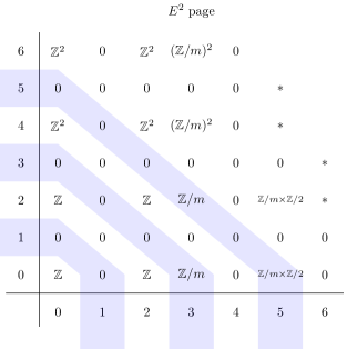
Figure 6: The $E^{2}$ page of the AHSS for spin_c bordism, for the fibration $\text{pt}\to B|\mathbb{G}|\to B|\mathbb{G}|$, where $\mathbb{G}$ is the 2-group $\text{U}(1)^{[0]}\times_{\hat{\kappa}}\text{U}(1)^{[1]}$ with $m:=|\hat{\kappa}|$. Up to the $p+q=6$ diagonal there are no non-vanishing differentials whatsoever, and the entries shown in this region stabilize to the last page.

Having already computed the integral homology (5.27) of $B|\mathbb{G}|$ in §5.2, and using the well-known result for the $\text{Spin}_{c}$-bordism groups of a point bahri1987eta (see the first row in Table 2), it is straightforward to use the AHSS

$$E^{2}_{p,q}=H^{p}\big{(}B|\mathbb{G}|;\Omega^{\text{Spin}_{c}}_{q}(\text{pt})\big{)}\implies\Omega^{\text{Spin}_{c}}_{q}(B|\mathbb{G}|)$$ (6.15)

to compute the $\text{Spin}_{c}$ bordism groups of interest. The $E^{2}$ page is shown in Fig. 6. Things could not be much simpler; in the region of interest, all differentials are vanishing and all the elements on $E^{2}$ up to the $p+q=6$ diagonal stabilize to the last page. The bordism groups are recorded in the second row of Table 2. There is an extension problem that we cannot resolve using the AHSS for $\Omega_{5}$, but it is not relevant to our discussion here.

It is curious that $\Omega^{\text{Spin}_{c}}_{3}(B|\mathbb{G}|)\cong\mathbb{Z}/m$ compared to $\Omega^{\text{Spin}}_{3}(B|\mathbb{G}|)\cong\mathbb{Z}/(2m)$. One might naïvely expect the same classification because the anomaly coefficient $\mathcal{A}_{2}$ is shifted by $2n\hat{\kappa}$ for any $n\in\mathbb{Z}$ from the 2-group transformation of the Green–Schwarz counter-term $\text{i}n\int_{M_{2}}B^{(2)}$. The puzzle can be resolved by correctly identifying the four integers in $\Omega^{\text{Spin}_{c}}_{4}(B\text{U}(1))\cong\mathbb{Z}^{4}$ that properly classify all perturbative anomalies, before turning on the 2-group structure.

Let $F$ be the field strength for the background gauge field of the $\text{U}(1)$ 0-form global symmetry as before, and let $G$ denote the field strength associated to the $\text{Spin}_{c}$ connection. Consider $N$ left-moving fermions with charges $\{q_{i}\}$ under the ordinary $\text{U}(1)$ global symmetry and with charges $\{g_{i}\}$ under the $\text{Spin}_{c}$ connection. There is no constraint on the $q_{i}$, but the $g_{i}$ must all be odd integers. The anomaly polynomial associated to this matter content is given by

$$\Phi_{4}=\frac{1}{2}\sum_{i=1}^{N}q_{i}^{2}c_{1}(F)^{2}+\sum_{i=1}^{N}g_{i}q_{i}c_{1}(F)c_{1}(G)+\frac{1}{2}\sum_{i=1}^{N}g_{i}^{2}c_{1}(G)^{2}-N\frac{p_{1}(R)}{24},$$ (6.16)

where $p_{1}(R)$ is the first Pontryagin class of the tangent bundle. The four anomaly coefficients that accompany each term in $\Phi_{4}$ are not strictly independent from one another, so they cannot be taken as labels for each factor of $\mathbb{Z}$ in $\Omega^{\text{Spin}}_{4}(B\text{U}(1))$.

To extract a set of correct integer labels, we first choose an integral basis for the anomaly polynomial in terms of linear combinations of $c_{1}(F)^{2}$, $c_{1}(F)c_{1}(G)$, $c_{1}(G)^{2}$, and $p_{1}(R)$. One option is

$$\alpha_{1}=c_{1}(F)^{2},\quad\alpha_{2}=\frac{1}{2}c_{1}(F^{2})+c_{1}(F)c_{1}(G),\quad\alpha_{3}=\frac{1}{2}c_{1}(G)^{2}-\frac{p_{1}(R)}{24},\quad\alpha_{4}=\frac{p_{1}(R)}{3}.$$ (6.17)

We know that $\alpha_{4}$ is integral because $\int_{M_{4}}p_{1}(R)/3$ is just the signature of $M_{4}$ which is integral (and takes a minimal value of $1$, e.g. on $M_{4}=\mathbb{C}P^{2}$) for any orientable 4-manifold $M_{4}$. To see the integrality of $\alpha_{3}$, we apply the Atiyah–Singer index theorem for a $\text{Spin}_{c}$ connection coupled to a single left-moving fermion with $q=0$ and $g=1$. Next, applying the same index theorem to a single left-moving fermion with $q=1$ and $g=1$ tells us that $\alpha_{2}$ is an integer. Finally, the class $\alpha_{1}$ is integral by definition, and indeed it takes a minimal value of $1$. To see this, take $M_{4}=\mathbb{C}P^{2}$ with $F$ such that $\int F/2\pi=1$ on a $\mathbb{C}P^{1}$ subspace. Hence $c_{1}(F)$ is the generator $x$ of $H^{2}(\mathbb{C}P^{2};\mathbb{Z})$, so $c_{1}(F)^{2}=x^{2}=1\in H^{4}(\mathbb{C}P^{2};\mathbb{Z})$ generates the top cohomology, which evaluates to 1 on the fundamental class $[\mathbb{C}P^{2}]$.

In terms of these basis elements, the anomaly polynomial can be written as $\Phi_{4}=\sum_{i=1}^{4}n_{i}\alpha_{i}$, where the variables $n_{i}$ are

$$n_{1}=\frac{1}{2}\sum_{i=1}^{N}q_{i}(q_{i}-g_{i}),\quad n_{2}=\sum_{i=1}^{N}q_{i}g_{i},\quad n_{3}=\sum_{i=1}^{N}g_{i}^{2},\quad n_{4}=\frac{1}{8}\sum_{i=1}^{N}(g_{i}^{2}-1),$$ (6.18)

and our arguments above tell us that each $n_{i}$ must be an integer. This is clearly the case for $n_{2}$ and $n_{3}$. To see that $n_{1}$ is an integer, recall that $g_{i}$ are all odd. So when $q_{i}$ is odd, $(q_{i}-g_{i})$ is even, and vice versa. So their product must be even. Similarly, to see that $n_{4}$ is an integer, we observe that $g_{i}-1$ and $g_{i}+1$ are both even and differ by 2, so one of them must be divisible by $4$. Hence their product is divisible by $8$.

When we turn the 2-group structure back on, the shift in anomaly coefficients induced by the Green–Schwarz $S\supset\text{i}n\int_{M_{2}}B^{(2)}$ counter-term amounts to a shift

$$n_{1}\mapsto n_{1}+n\hat{\kappa}.$$ (6.19)

It is now obvious that the local anomaly labelled by the integer $n_{1}$ is truncated down to a mod $|\hat{\kappa}|$ anomaly. If one first takes care to cancel the anomalies involving the $\text{Spin}_{c}$ connection, which amounts to choosing charges $\{g_{i}\}$ such that $n_{2}$, $n_{3}$, and $n_{4}$ vanish, then we find that the 2-group structure can indeed be used to completely capture the remaining ’t Hooft anomaly in the ordinary $\text{U}(1)^{(0)}$ 0-form global symmetry, in the sense proposed by Sharpe Sharpe:2015mja . This should be contrasted with the residual order 2 anomaly (6.7) that cannot be cancelled in this way for the theory defined with a spin structure.

7 Conclusion and outlook

In this paper, we explored anomalies in 2-group global symmetries $\mathbb{G}$ in field theories in $d=4$ and $d=2$ dimensions using the cobordism classification. We compute the bordism groups $\Omega^{H}_{d+1}(B|\mathbb{G}|)$ and $\Omega^{H}_{d+2}(B|\mathbb{G}|)$ of the classifying space $B|\mathbb{G}|$ of the nerve of $\mathbb{G}$, with the tangential structure $H=\text{SO}$ or Spin. The torsion part of the former group gives us the global anomaly while the free part of the latter gives the perturbative anomaly. Throughout the work, we focus on 2-groups $\mathbb{G}$ whose 0-form and 1-form symmetry parts are compact, connected abelian groups ergo tori, which we refer to as ‘toric 2-groups’.

As a warm-up example, we first looked at Maxwell’s theory in 4d, on a general orientable manifold (not necessarily spin). The 2-group symmetry in this theory contains only the 1-form symmetry part, being a product of the $\text{U}(1)$ electric 1-form symmetry and the $\text{U}(1)$ magnetic 1-form symmetry. The familiar mixed anomaly Gaiotto:2014kfa between these two $\text{U}(1)$ factor can be given in terms of a bordism invariant in the free part of $\Omega_{6}$. There are also three global anomalies, probed by the torsion subgroup of $\Omega_{5}$, which can only be seen on non-spin manifolds and can be interpreted as mixed anomalies between the 1-form symmetries and gravity. We also studied anomalies when one of the $\text{U}(1)$ factor breaks explicitly to its cyclic subgroup due to the presence of a charged scalar, and related them to anomalies in pure Maxwell’s theory via anomaly interplay.

When both the 0-form and 1-form symmetry constituents of $\mathbb{G}$ are $\text{U}(1)$, with the Postnikov class given by $\hat{\kappa}\in\mathbb{Z}$, we used a variety of techniques to prove that the relevant spin bordism groups are

$$\Omega^{\text{Spin}}_{5}(B|\mathbb{G}|)\cong\mathbb{Z}/|\hat{\kappa}|,\quad\operatorname*{Hom}\left(\Omega^{\text{Spin}}_{6}(B|\mathbb{G}|),\mathbb{Z}\right)\cong\mathbb{Z}\;.$$ (7.1)

The free part of the sixth bordism group signals the existence of a perturbative anomaly in 4d, which is just the mixed anomaly between the $\text{U}(1)$ 0-form symmetry and gravity. On the other hand, the perturbative cubic anomaly for $\text{U}(1)$ 0-form symmetry that would be there were $\hat{\kappa}$ to vanish now transmutes into a discrete global anomaly captured by the torsion part of the 5th bordism group. These cobordism computations are in perfect agreement with the physics argument put forward by Córdova, Dumitrescu, and Intriligator Cordova:2018cvg .

We next discussed the fate of anomalies for a $\text{U}(1)$ 0-form symmetry in 2d, for both spin and non-spin manifolds. We revisited the construction, originally due to Sharpe Sharpe:2015mja , whereby this 0-form symmetry is enhanced to a 2-group symmetry by mixing it with a $\text{U}(1)$ 1-form symmetry whose current is given by the top form on the underlying manifold. When the anomaly coefficient $\mathcal{A}_{2}$ for the pure $\text{U}(1)$ anomaly is even, we found that, by choosing the Postnikov class of the enhanced 2-group to be $\hat{\kappa}=\mathcal{A}_{2}/2$, the anomaly can be fully absorbed away. On the other hand, in the presence of the spin structure, when $\mathcal{A}_{2}$ is odd and restricting to spin-manifolds, the most one can do is reduce the anomaly down to an order 2 discrete anomaly, that we intrepret as an anomaly in the spin structure.

There are many future directions to pursue that are natural extensions of this work. One obvious alley is to look at more general classes of 2-group beyond our ‘toric’ assumption, e.g. 2-groups whose 0-form symmetry is a non-abelian Lie group, and/or 2-groups whose 0-form or 1-form symmetry is a finite group Benini:2018reh ; DelZotto:2020sop ; Apruzzi:2021vcu ; Bhardwaj:2021wif ; Apruzzi:2021mlh ; Lee:2021crt ; DelZotto:2022fnw ; DelZotto:2022joo ; Bhardwaj:2022scy ; Carta:2022fxc . One can rigorously analyse anomalies in these 2-group symmetries using the cobordism classification. Doing so involves an extension of the mathematical machinery developed in this paper, and would offer a non-trivial check on other methods of seeing the anomalies that have been explored recently in the literature Bhardwaj:2022dyt . One can also study how these anomalies relate to the anomalies studied in this paper through a generalised version of anomaly interplay.

Another avenue to pursue concerns a higher-dimensional generalisation of the 2d 2-groups discussed in § 6, as follows. We saw that one can cancel (almost) all pure $\text{U}(1)$ anomalies in 2d by enhancing the $\text{U}(1)$ 0-form symmetry to a 2-group by making use of the top-form $\text{U}(1)$ current. One then wonders whether there is an analogous story for ‘top-group’ symmetry structures in higher dimensions, e.g. 4-group symmetry in 4d, in which a ‘topological 3-form symmetry’ with $j_{4}=\text{vol}_{4}$ is fused with the ordinary 0-form symmetry to kill the cubic anomaly. Moreover, the remnant order 2 anomaly in the 2d case is a direct result of the non-trivial role played by the spin structure. It remains to be seen whether such an interplay between ‘top-group’ symmetries and spin-structure anomalies persists in higher dimensions.

For all these anomalies, there is of course a dual interpretation concerning symmetry protected topological (SPT) phases of matter that are protected by these generalised symmetry types, which are rigorously classified by cobordism. Furthermore, it is conceivable that by extending the bordism computations to more generalised symmetries one could uncover novel anomalies/phases, and suggest corresponding new constraints on the dynamics of theories with such symmetry.

Appendix A Additional cohomology computations

In this Appendix, we collect results and computations for various cohomology groups.

A.1 Cohomology groups of Eilenberg–Maclane spaces

In this Subsection, we collect classic results for cohomology groups of various Eilenberg–Maclane spaces $K(G,n)$. The mod 2 cohomology results below are obtained by Serre in the classic paper Serre1953aP .

$K(\mathbb{Z}/2,2)$

The mod 2 cohomology ring of an Eilenberg–Maclane space $B^{2}\mathbb{Z}/2=K(\mathbb{Z}/2,2)$ is given by

$$H^{\bullet}(K(\mathbb{Z}/2,2);\mathbb{Z}/2)\cong\mathbb{Z}/2[u_{2},\text{~{}Sq}^{1}u_{2},\text{~{}Sq}^{2}\text{~{}Sq}^{1}u_{2},\ldots,\text{~{}Sq}^{2^{k}}\text{~{}Sq}^{2^{k-1}}\ldots\text{~{}Sq}^{2}\text{~{}Sq}^{1}u_{2},\ldots],$$ (A.1)

where $u_{2}$ is the unique generator in $H^{2}$.

$K(\mathbb{Z},2)$

The classifying space $B\text{U}(1)$ of $\text{U}(1)$ is a $K(\mathbb{Z},2)$ space. We have

$$H^{\bullet}(K(\mathbb{Z},2);\mathbb{Z})=H^{\bullet}(B\text{U}(1);\mathbb{Z})\cong\mathbb{Z}[c_{1}],$$ (A.2)

where $c_{1}$ is the unique generator in $H^{2}$ called the universal first Chern class. The mod 2 version is given simply by

$$H^{\bullet}(K(\mathbb{Z},2);\mathbb{Z}/2)\cong\mathbb{Z}/2[c_{1}],$$ (A.3)

where $c_{1}$ is now the mod 2 reduction of the universal first Chern class. The action of the Steenrod squares are given by $\text{~{}Sq}^{1}c_{1}=0$, $\text{~{}Sq}^{2}c_{1}=c_{1}^{2}$ which follows directly from the axioms.

$K(\mathbb{Z},3)$

The mod 2 cohomology ring of an Eilenberg–Maclane space $K(\mathbb{Z},3)$ is given by

$$H^{\bullet}\left(K(\mathbb{Z},3);\mathbb{Z}/2\right)\cong\mathbb{Z}/2[\tau_{3},\text{Sq}^{2}\tau_{3},\text{Sq}^{4}\text{Sq}^{2}\tau_{3},\text{Sq}^{8}\text{Sq}^{4}\text{Sq}^{2}\tau_{3},\ldots],$$ (A.4)

where $\tau_{3}$ is the unique generator in $H^{3}(K(\mathbb{Z},3);\mathbb{Z}/2)$.

Integral cohomology groups of $K(\mathbb{Z},3)$ can be obtained by applying the universal coefficient theorem to the homology groups computed in Ref. breen2014derived . The resulting cohomology groups are shown in Table 3 below.

$n$	$0$	$1$	$2$	$3$	$4$	$5$	$6$	$7$	$8$
$H^{n}(K(\mathbb{Z},3);\mathbb{Z})$	$\mathbb{Z}$	$0$	$0$	$\mathbb{Z}$	$0$	$0$	$\mathbb{Z}/2$	$0$	$\mathbb{Z}/3$

Table 3: Integral cohomology groups up to degree 8 of $K(\mathbb{Z},3)$

A.2 Mod 2 cohomology ring of the classifying space of an abelian 2-group

In this Subsection, we use the Serre spectral sequence to calculate the mod 2 cohomlogy ring of $B|\mathbb{G}|$ when $\mathbb{G}$ is the abelian 2-group $\text{U}(1)^{[0]}\times_{\hat{\kappa}}\text{U}(1)^{[1]}$ studied in §5.2 with the Postnikov class $\hat{\kappa}$.

The cohomological Serre spectral sequence induced by the fibration $K(\mathbb{Z},3)\to B|\mathbb{G}|\to K(\mathbb{Z},2)$ is

$$E_{2}^{p,q}=H^{p}\left(K(\mathbb{Z},2);H^{q}\left(K(\mathbb{Z},3);\mathbb{Z}/2\right)\right)\Rightarrow H^{p+q}\left(B|\mathbb{G}|;\mathbb{Z}/2\right).$$ (A.5)

The entries on the $E_{2}$ page can be computed from the results given in §A.1. There is no non-trivial differentials on the $E_{2}$ or $E_{3}$ pages in the range of degrees we are interested in, and the $E_{2}$ entries in this range propagate to the $E_{4}$ page, shown in Fig. 7. As explained in §5.2, the differentials $\alpha$ and $\beta$ on the $E_{4}$ page are given by contraction with the Postnikov class $\hat{\kappa}$. Thus, they are non-trivial if and only if $\hat{\kappa}$ is odd. In this case, the resulting $E_{5}$ page is shown on the right-hand side of Fig. 7. When $\hat{\kappa}$ is even, the entries stabilise already on the The entries in the range of interest stabilise on this page. On the other hand, when $\hat{\kappa}$ is even, the entries stabilise already on the $E_{4}$ page. In either case, we can read off the mod 2 cohomology groups to be

$n$	$0$	$1$	$2$	$3$	$4$	$5$	$6$
$H^{n}(B|\mathbb{G}|;\mathbb{Z}/2)$,  $\hat{\kappa}$ odd	$\mathbb{Z}/2$	$0$	$\mathbb{Z}/2$	$0$	$0$	$\mathbb{Z}/2$	$\mathbb{Z}/2$
$H^{n}(B|\mathbb{G}|;\mathbb{Z}/2)$,  $\hat{\kappa}$ even	$\mathbb{Z}/2$	$0$	$\mathbb{Z}/2$	$\mathbb{Z}/2$	$\mathbb{Z}/2$	$\mathbb{Z}/2\times\mathbb{Z}/2$	$\mathbb{Z}/2\times\mathbb{Z}/2$

Table 4: The mod 2 cohomology groups of $B|\mathbb{G}|$ where $\mathbb{G}$ is the 2-group $\text{U}(1)^{[0]}\times_{\hat{\kappa}}\text{U}(1)^{[1]}$ with the Postnikov class $\hat{\kappa}$

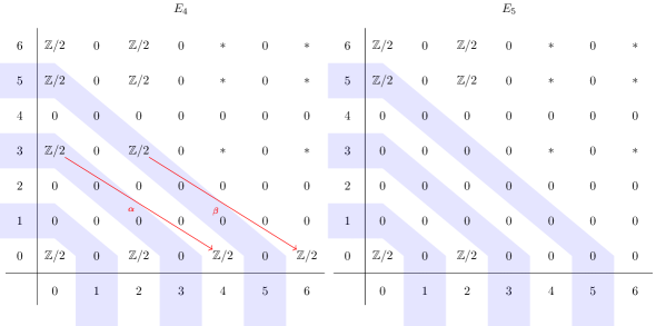
Figure 7: The Serre spectral sequence for the mod 2 cohomology for $B|\mathbb{G}|$ when $\mathbb{G}=\text{U}(1)^{[0]}\times_{\hat{\kappa}}\text{U}(1)^{[1]}$ with an odd Postnikov class $\hat{\kappa}$.

On the pages of the Serre spectral sequence, there are non-trivial $\text{~{}Sq}^{2}$ actions on the mod 2 cohomology rings of the fibre $K(\mathbb{Z},3)$ and the base $K(\mathbb{Z},2)$ that converge to $\text{~{}Sq}^{2}$ actions on $H^{\bullet}\left(B|\mathbb{G}|;\mathbb{Z}/2\right)$ (Theorem 6.15 of McCleary2000aB ). In particular, in the even $\hat{\kappa}$ case, we have

$$\begin{split}\text{~{}Sq}^{2}:H^{2}\left(B|\mathbb{G}|;\mathbb{Z}/2\right)&\to H^{4}\left(B|\mathbb{G}|;\mathbb{Z}/2\right)\\ c_{1}&\mapsto c_{1}^{2}\end{split}$$ (A.6)

and

$$\begin{split}\text{~{}Sq}^{2}:H^{3}\left(B|\mathbb{G}|;\mathbb{Z}/2\right)&\to H^{5}\left(B|\mathbb{G}|;\mathbb{Z}/2\right)\\ \tau_{3}&\mapsto\text{~{}Sq}^{2}\tau_{3}\end{split}$$ (A.7)

where $c_{1}$, $\tau_{3}$, $c_{1}^{2}$, and $\text{~{}Sq}^{2}\tau_{3}$, are now taken to be the unique generators for $H^{i}(B|\mathbb{G}|;\mathbb{Z}/2)$, $i=2,3,4,5$, respectively.

Appendix B Additional bordism calculations

B.1 Maxwell

Here we compute the bordism groups for the symmetry type

$$H=\text{SO}\times\mathbb{G},\qquad B|\mathbb{G}|=B^{2}\text{U}(1)_{e}\times B^{2}\text{U}(1)_{m}\,,$$ (B.1)

relevant to ‘free Maxwell theory’, i.e. $\text{U}(1)$ gauge group with no dynamical matter, which has intact electric and magnetic $\text{U}(1)$ 1-form global symmetries, discussed in §4. Since $\text{U}(1)\cong S^{1}\cong B\mathbb{Z}$, the classifying space for a $U(1)$ 1-form symmetry $B^{2}\text{U}(1)\cong K(\mathbb{Z},3)$ is an Eilenberg–Maclane space whose cohomology is known. Using the Künneth theorem we find the integral homology of $B|\mathbb{G}|=B^{2}\text{U}(1)\times B^{2}\text{U}(1)$, as recorded in Table 5. We also need the oriented bordism groups of a point 10.2307/1970136 , which are recorded in Table 6.

$i$	0	1	2	3	4	5	6	7
$H_{i}(K(\mathbb{Z},3);\mathbb{Z})$	$\mathbb{Z}$	$0$	$0$	$\mathbb{Z}$	$0$	$\mathbb{Z}/2$	$0$	$\mathbb{Z}/3$
$H_{i}(K(\mathbb{Z},3);\mathbb{Z}/2)$	$\mathbb{Z}/2$	$0$	$0$	$\mathbb{Z}/2$	$0$	$\mathbb{Z}/2$	$\mathbb{Z}/2$	$0$
$H_{i}((B^{2}\text{U}(1))^{2};\mathbb{Z})$	$\mathbb{Z}$	$0$	$0$	$\mathbb{Z}^{2}$	$0$	$(\mathbb{Z}/2)^{2}$	$\mathbb{Z}$	$(\mathbb{Z}/3)^{2}$
$H_{i}((B^{2}\text{U}(1))^{2};\mathbb{Z}/2)$	$\mathbb{Z}/2$	$0$	$0$	$(\mathbb{Z}/2)^{2}$	$0$	$(\mathbb{Z}/2)^{2}$	$(\mathbb{Z}/2)^{3}$	$0$

Table 5: Integral and mod 2 homology groups of $(B^{2}\text{U}(1))^{2}=\left(K(\mathbb{Z},3)\right)^{2}$, relevant to Maxwell theory.

$i$	$0$	$1$	$2$	$3$	$4$	$5$	$6$	$7$	$8$
$\Omega^{\text{SO}}_{i}(\text{pt})$	$\mathbb{Z}$	$0$	$0$	$0$	$\mathbb{Z}$	$\mathbb{Z}/2$	$0$	$0$	$\mathbb{Z}^{2}$

Table 6: Oriented bordism groups for a point 10.2307/1970136 .

We next write down the AHSS for oriented bordism associated to the trivial fibration of $|\mathbb{G}|$ by a point, for which the second page is given by

$$E^{2}_{p,q}=H_{p}\left((B^{2}\text{U}(1))^{2};\Omega_{q}^{\text{SO}}(\text{pt})\right)\,.$$ (B.2)

This is shown in Fig. 8.

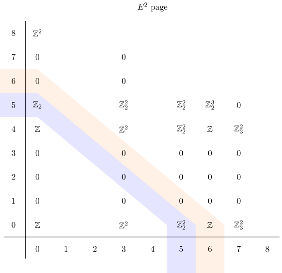
Figure 8: The second page of the AHSS for $\Omega^{\text{SO}}_{\bullet}\left((B^{2}\text{U}(1))^{2}\right)$.

We want to read off the fifth and sixth bordism groups, which receive contributions from the $p+q=5$ (blue) and $p+q=6$ (orange) diagonals respectively. For the sixth bordism group, there is a single factor $E^{2}_{6,0}=\mathbb{Z}$ to consider. The only possible differential is $d^{5}:E^{5}_{6,0}\to E^{5}_{0,5}\cong\mathbb{Z}/2$, whose kernel is obviously isomorphic to $\mathbb{Z}$, meaning that $E^{\infty}_{6,0}=\mathbb{Z}$. Thus,

$$\Omega^{\text{SO}}_{6}\left((B^{2}\text{U}(1))^{2}\right)=\mathbb{Z}\,.$$ (B.3)

For the fifth bordism group, the $E^{2}_{5,0}=(\mathbb{Z}/2)^{2}$ element stabilizes to the last page, because the only possible differential is $d^{4}:E^{4}_{5,0}\to E^{4}_{0,4}:\mathbb{Z}/2\mapsto\mathbb{Z}$ which is therefore the zero map. For the $E^{2}_{0,5}$ element, it is again the $d^{5}:E^{5}_{6,0}\to E^{5}_{0,5}$ map that is important. We can in fact deduce that this differential must be zero simply because it hits the zeroth column which records the bordism groups of a point, and since there is a canonical split $\Omega^{\text{SO}}_{\bullet}(X)\cong\Omega^{\text{SO}}_{\bullet}(\text{pt})\oplus\widetilde{\Omega}^{\text{SO}}_{\bullet}(X)$ for $X$ connected, where the second factor is the reduced bordism of $X$, the $E_{0,5}$ factor must stabilize to the last page. This also makes it obvious that there can be no non-trivial extension, and so we can read off

$$\Omega^{\text{SO}}_{5}\left((B^{2}\text{U}(1))^{2}\right)=(\mathbb{Z}/2)^{3}\,.$$ (B.4)

It is easy to read off the lower-degree bordism groups too, and we summarize the results in Table 7.

$i$	$0$	$1$	$2$	$3$	$4$	$5$	$6$
$\Omega^{\text{SO}}_{i}\left((B^{2}U(1))^{2}\right)$	$\mathbb{Z}$	$0$	$0$	$\mathbb{Z}^{2}$	$\mathbb{Z}$	$(\mathbb{Z}/2)^{3}$	$\mathbb{Z}$

Table 7: Oriented bordism groups up to degree 6, for a pair of $\text{U}(1)$ 1-form symmetries.

B.2 Scalar QED with charge-2 boson

Next we compute the bordism groups for

$$H=\text{SO}\times\mathbb{G}^{\prime},\qquad B|\mathbb{G}^{\prime}|=B^{2}\mathbb{Z}/2_{e}\times B^{2}\text{U}(1)_{m}\,,$$ (B.5)

relevant to QED with a charge-2 boson, which has the effect of breaking the $\text{U}(1)_{e}$ 1-form symmetry down to a discrete $\mathbb{Z}/2_{e}$ subgroup. Using the Künneth theorem we find the integral homology of $B^{2}\mathbb{Z}/2\times B^{2}\text{U}(1)$, as recorded in Table 8.

$i$	0	1	2	3	4	5	6	7
$H_{i}(B^{2}\mathbb{Z}/2;\mathbb{Z})$	$\mathbb{Z}$	$0$	$\mathbb{Z}/2$	$0$	$\mathbb{Z}/4$	$\mathbb{Z}/2$	$\mathbb{Z}/2$	$\mathbb{Z}/2$
$H_{i}(B^{2}\mathbb{Z}/2;\mathbb{Z}/2)$	$\mathbb{Z}/2$	$0$	$\mathbb{Z}/2$	$\mathbb{Z}/2$	$\mathbb{Z}/2$	$(\mathbb{Z}/2)^{2}$	$(\mathbb{Z}/2)^{2}$	$(\mathbb{Z}/2)^{2}$
$H_{i}(B^{2}\mathbb{Z}/2\times B^{2}\text{U}(1);\mathbb{Z})$	$\mathbb{Z}$	$0$	$\mathbb{Z}/2$	$\mathbb{Z}$	$\mathbb{Z}/4$	$(\mathbb{Z}/2)^{3}$	$\mathbb{Z}/2$	${\scriptstyle(\mathbb{Z}/2)^{2}\times\mathbb{Z}/3\times\mathbb{Z}/4}$
$H_{i}(B^{2}\mathbb{Z}/2\times B^{2}\text{U}(1);\mathbb{Z}/2)$	$\mathbb{Z}/2$	$0$	$\mathbb{Z}/2$	$(\mathbb{Z}/2)^{2}$	$\mathbb{Z}/2$	$(\mathbb{Z}/2)^{4}$	$(\mathbb{Z}/2)^{4}$	$(\mathbb{Z}/2)^{4}$

Table 8: Integral and mod 2 homology groups of $B^{2}\mathbb{Z}/2$ and $B^{2}\mathbb{Z}/2\times B^{2}\text{U}(1)$. Recall the homology of $B^{2}\text{U}(1)$ is recorded in the first two lines of Table 5.

We next write down the AHSS for oriented bordism associated to the trivial fibration $\text{pt}\to B^{2}\mathbb{Z}/2\times B^{2}\text{U}(1)\to B^{2}\mathbb{Z}/2\times B^{2}\text{U}(1)$, for which the second page is given by (see Fig. 9),

$$E^{2}_{p,q}=H_{p}\left(B^{2}\mathbb{Z}/2\times B^{2}\text{U}(1);\Omega_{q}^{\text{SO}}(\text{pt})\right)\,.$$ (B.6)

Figure 9: The second page of the AHSS for $\Omega^{\text{SO}}_{\bullet}\left(B^{2}\mathbb{Z}/2\times B^{2}\text{U}(1)\right)$.

We want to read off $\Omega_{5}$ and $\Omega_{6}$ from the stabilization of elements on the $p+q=5$ and $p+q=6$ diagonals respectively. For the fifth bordism group, very similar arguments to those of B.1 tell us that $E_{5,0}^{\infty}=(\mathbb{Z}/2)^{3}$ and $E_{0,5}^{\infty}=\mathbb{Z}/2$, and the canonical split $\Omega^{\text{SO}}_{\bullet}(X)\cong\Omega^{\text{SO}}_{\bullet}(\text{pt})\oplus\widetilde{\Omega}^{\text{SO}}_{\bullet}(X)$ again tells us that the extension problem is trivial, giving:

$$\Omega^{\text{SO}}_{5}\left(B^{2}\mathbb{Z}/2\times B^{2}\text{U}(1)\right)=(\mathbb{Z}/2)^{4}\,.$$ (B.7)

For $\Omega_{6}$, there is a potentially non-vanishing differential on the fifth page, $d^{5}:E_{7,0}\to E_{2,5}:(\mathbb{Z}/2)^{2}\times\mathbb{Z}/3\times\mathbb{Z}/4\mapsto\mathbb{Z}/2$. Without knowing this differential, one cannot read off $\Omega_{6}$ – the most we can conclude is that it equals $\mathbb{Z}/2$, $\mathbb{Z}/4$, or $\mathbb{Z}/2\times\mathbb{Z}/2$. In any case, we have that $\Omega^{\text{SO}}_{6}\left(B^{2}\mathbb{Z}/2\times B^{2}\text{U}(1)\right)$ is pure torsion, which is all that’s relevant for discussing the corresponding anomalies in 4d.

Appendix C Computation of a key differential

This Appendix is written by Arun Debray.

In this appendix, we finish the computation from §5.2.3, showing that if $\mathbb{G}$ is a $2$-group with 0- and 1-form parts both $\text{U}(1)$ and $k$-invariant equal to $m$ times the generator of $H^{4}(B\text{U}(1);\mathbb{Z})\cong\mathbb{Z}$, where $m$ is odd, then $\Omega_{5}^{\text{Spin}}(B|\mathbb{G}|)\cong\mathbb{Z}/m$. After the calculation in §5.2.3, the only ambiguity is in the $2$-torsion, which could be either $0$ or $\mathbb{Z}/2$, depending on the value of a $d_{3}$ in the Atiyah-Hirzebruch spectral sequence in Fig. 5. This differential resisted several of our standard techniques to address it, as did an analogous differential in the Adams spectral sequence computing the $2$-completion of $\Omega_{5}^{\text{Spin}}(B|\mathbb{G}|)$.

Here we finish the computation of the $2$-torsion subgroup of $\Omega_{5}^{\text{Spin}}(B|\mathbb{G}|)$ in a different way, resolving the differentials only implicitly. Specifically, we fit $\Omega_{\bullet}^{\text{Spin}}(B|\mathbb{G}|)$ into a long exact sequence (C.2) and compute enough other terms in the long exact sequence to determine $\Omega_{5}^{\text{Spin}}(B|\mathbb{G}|)$. This long exact sequence is a version of the Gysin sequence for spin bordism, and one of its homomorphisms has a geometric interpretation as a Smith homomorphism, a map between bordism groups defined by sending a manifold $M$ to a smooth representative of the Poincaré dual to a characteristic class of $M$. The general version of (C.2) was written down in Debray:2023yrs to study Smith homomorphisms and their applications to anomalies of quantum field theories; see there and Cordova:2019wpi ; Hason:2020yqf for more on Smith homomorphisms and their role in physics.

Theorem C.1 (Debray:2023yrs ).

Let $V\to X$ be a vector bundle of rank $r$ over a CW complex $X$, $\pi\colon S(V)\to X$ be the sphere bundle of $V$, $X^{V-r}$ be the Thom spectrum of the rank-zero virtual vector bundle $V-\underline{\mathbb{R}}^{r}$, and $E_{\bullet}$ be a generalised homology theory. Then there is a long exact sequence

$$\dotsb\longrightarrow E_{n}(S(V))\overset{\pi_{*}}{\longrightarrow}E_{n}(X)\overset{\psi}{\longrightarrow}E_{n-r}(X^{V-r})\longrightarrow E_{n-1}(S(V))\longrightarrow\dots$$ (C.1)

The map $\psi$ is the Smith homomorphism, but we will not need that fact; see Debray:2023yrs for more information.

Proof.

We will show that the Thom space $\mathrm{Th}(X,V)$ of $V$ is the homotopy cofibre of $\pi$, so there is the Puppe long exact sequence $\dotsb\to E_{n}(S(V))\to E_{n}(X)\to\widetilde{E}_{n}(\mathrm{Th}(X,V))\to E_{n-1}(S(V))\to\dotsb$. Once this is established, (C.1) follows: $X^{V-r}\simeq\Sigma^{-r}\Sigma^{\infty}_{+}\mathrm{Th}(X,V)$, and $\Sigma_{+}^{\infty}$ induces an isomorphism for any generalised homology theory and $\Sigma^{-r}$ shifts generalised homology down in grading by $r$, yielding (C.1).

The homotopy cofibre of an inclusion $A\hookrightarrow X$ of CW complexes such that the image of $A$ is a union of cells is the quotient $X/A$; in general, one can compute the homotopy cofibre of a map $f\colon A\to X$ between CW complexes by changing $f$ and $X$ by a homotopy so that $f$ is indeed a cellular inclusion. For $\pi\colon S(V)\to X$ from the theorem statement, replace $\pi$ with the inclusion $i\colon S(V)\hookrightarrow D(V)$ of $S(V)$ into the disc bundle $D(V)$ of $V\to X$; the map $\pi^{\prime}\colon D(V)\to X$ is a homotopy equivalence and $\pi^{\prime}\circ i=\pi$, and the CW structures on $X$ and the standard CW structure on $D^{n}$ can be used to put CW structures on $S(V)$ and $D(V)$ such that the image of $i$ is a union of cells. Thus the homotopy cofibre of $\pi\colon S(V)\to V$ is the quotient $D(V)/S(V)$, which is by definition $\mathrm{Th}(X,V)$. ∎

We are interested in $E_{\bullet}=\Omega_{\bullet}^{\text{Spin}}$, and specifically in $2$-torsion. To avoid worrying about torsion for other primes, we localise at $2$, meaning we tensor with the ring $\mathbb{Z}_{(2)}$ of rational numbers whose denominators in lowest terms are odd. If $A$ is a finitely generated abelian group, so that $A$ is a direct sum of a free abelian group $\mathbb{Z}^{r}$ and cyclic groups $\mathbb{Z}/p_{i}^{e_{i}}$ of prime-power order, localising at $2$ has the effect of replacing $\mathbb{Z}^{r}$ with $(\mathbb{Z}_{(2)})^{r}$, preserving all $2^{e_{i}}$-torsion, and sending all odd-prime-power torsion to zero. Since we are trying to determine the $2$-torsion subgroup of $\Omega_{5}^{\text{Spin}}(B|\mathbb{G}|)$, which is a finitely generated abelian group, we lose no relevant information by localising at $2$. Moreover, since $\mathbb{Z}_{(2)}$ is a flat ring, tensoring with $\mathbb{Z}_{(2)}$ preserves long exact sequences (i.e. $2$-localisation is exact), so we can still apply (C.1) after $2$-localising.

For any $2$-group $\mathbb{H}$, the classifying space $B|\mathbb{H}|$ has a CW structure (e.g. because it is the geometric realization of a simplicial space), so we can invoke Theorem C.1 for $X=B|\mathbb{G}|$. Quotienting $\mathbb{G}$ by its 1-form symmetry defines a map to the 0-form part of $\mathbb{G}$, which on classifying spaces induces a map $q\colon B|\mathbb{G}|\to B\text{U}(1)$. Let $V\to B|\mathbb{G}|$ be the pullback of the tautological complex line bundle $L\to B\text{U}(1)$ by $q$. Then Theorem C.1, together with exactness of $2$-localisation, gives us a long exact sequence

$$\dotsb\to\Omega_{5}^{\text{Spin}}(S(V))\otimes\mathbb{Z}_{(2)}\to\Omega_{5}^{\text{Spin}}(B|\mathbb{G}|)\otimes\mathbb{Z}_{(2)}\to\Omega_{3}^{\text{Spin}}((B|\mathbb{G}|)^{V-2})\otimes\mathbb{Z}_{(2)}\to\dots$$ (C.2)

We will show in Theorem C.3 that $\Omega_{5}^{\text{Spin}}(S(V))\otimes\mathbb{Z}_{(2)}$ and $\Omega_{3}^{\text{Spin}}((B|\mathbb{G}|)^{V-2})\otimes\mathbb{Z}_{(2)}$ both vanish; exactness then implies $\Omega_{5}^{\text{Spin}}(B|\mathbb{G}|)\otimes\mathbb{Z}_{(2)}=0$ as well, meaning $\Omega_{5}^{\text{Spin}}(B|\mathbb{G}|)$ has no $2$-torsion, which is what we want to prove in this appendix.

Before doing so, we first need to figure out what $S(V)$ is:

Lemma C.2.

The sphere bundle $S(V)$ is homotopy equivalent to $K(\mathbb{Z},3)$, and this homotopy equivalence identifies the bundle map $S(V)\to B|\mathbb{G}|$ with the map $K(\mathbb{Z},3)\to B|\mathbb{G}|$ given by inclusion of the 1-form $\text{U}(1)$ symmetry.

Proof.

Let $q\colon B|\mathbb{G}|\to B\text{U}(1)$ be the classifying map for $V$. Then the sphere bundle of $V$ is the pullback of the sphere bundle of the tautological line bundle $L\to B\text{U}(1)$, i.e. there is a homotopy pullback square

(C.3)

The sphere bundle of a complex line bundle is the associated principal $\text{U}(1)$-bundle; for $L\to B\text{U}(1)$, this is the tautological bundle $E\text{U}(1)\to B\text{U}(1)$, meaning $S(L)$ is contractible. In general, a homotopy pullback in which one of the two legs is contractible is the homotopy fibre (denoted $\mathrm{hofib}(\text{--})$) of the other leg, meaning the map $S(V)\to B|\mathbb{G}|$ can be identified with the canonical map $\mathrm{hofib}(q)\to B|\mathbb{G}|$. Recall that $q$ arose from a short exact sequence of topological groups

$$1\longrightarrow G\overset{i}{\longrightarrow}H\overset{p}{\longrightarrow}K\longrightarrow 1$$ (C.4)

by applying the classifying space functor; specifically, $G=|\text{U}(1)[1]|$, $H=|\mathbb{G}|$, and $K=\text{U}(1)$, and $q=Bp$. The classifying space functor turns short exact sequences of groups into fibre sequences of spaces, meaning that for (C.4) the homotopy fibre of $Bp$ is homotopy equivalent to $BG$, and this homotopy equivalence identifies the canonical map $\mathrm{hofib}(Bp)\to BH$ with $Bi\colon BG\to BH$. For our specific choices of $G$, $H$, and $K$, this tells us that up to homotopy equivalence, the map $S(V)\to B|\mathbb{G}|$ is the map $B|\text{U}(1)[1]|\simeq K(\mathbb{Z},3)\to B|\mathbb{G}|$ as claimed in the theorem statement. ∎

Lemma C.3.

$\Omega_{5}^{\text{Spin}}(K(\mathbb{Z},3))\otimes\mathbb{Z}_{(2)}$ and $\Omega_{3}^{\text{Spin}}((B|\mathbb{G}|)^{V-2})\otimes\mathbb{Z}_{(2)}$ both vanish.

Proof.

We check both of these using the Adams spectral sequence; the relevant differentials and extension questions are trivial for degree reasons, so these computations are straightforward analogues of Beaudry and Campbell’s computations in Ref. beaudry2018guide . We direct the reader to beaudry2018guide for more on our proof strategy and notation. The Adams spectral sequence computes $2$-completed spin bordism, not $2$-localised spin bordism, but because $\Omega_{5}^{\text{Spin}}(K(\mathbb{Z},3))$ and $\Omega_{3}^{\text{Spin}}((B|\mathbb{G}|)^{V-2})$ are finitely generated abelian groups, this distinction is not important: the $2$-localisation of a finitely generated abelian group $A$ vanishes if and only if the $2$-completion of $A$ vanishes, if and only if $A$ lacks both free and $2$-torsion summands.

For $K(\mathbb{Z},3)$, we need as input the $\mathcal{A}(1)$-module structure on $H^{\bullet}(K(\mathbb{Z},3);\mathbb{Z}/2)$ in degrees $6$ and below. This was computed by Serre (Serre1953aP, , §10): $H^{\bullet}(K(\mathbb{Z},3);\mathbb{Z}/2)$ is a polynomial algebra on generators $\tau_{3}$ in degree $3$, $\mathrm{Sq}^{2}\tau_{3}$ in degree $5$, and other generators in degrees too high to matter to us. Using this, one can compute that if $Q$ denotes the $\mathcal{A}(1)$-module $\mathcal{A}(1)/(\mathrm{Sq}^{1},\mathrm{Sq}^{2}\mathrm{Sq}^{3})$, then there is an isomorphism of $\mathcal{A}(1)$-modules

$$H^{\bullet}(K(\mathbb{Z},3);\mathbb{Z}/2)\cong{\color[rgb]{0.72,0,0}\mathbb{Z}/2}\oplus{\color[rgb]{0,0.44,0.57}\Sigma^{3}\raisebox{0.0pt}{\rotatebox{180.0}{$Q$}}}\oplus P,$$ (C.5)

where $P$ is concentrated in degrees $7$ and above, hence is irrelevant for our computation. We draw this decomposition in Fig. 10, left. Liulevicius (Liu62, , Theorem 3) computes $\operatorname*{Ext}_{\mathcal{A}(1)}({\color[rgb]{0.72,0,0}\mathbb{Z}/2})$ and Beaudry–Campbell (beaudry2018guide, , Figure 29) compute $\operatorname*{Ext}_{\mathcal{A}(1)}({\color[rgb]{0,0.44,0.57}\raisebox{0.0pt}{\rotatebox{180.0}{$Q$}}})$, so we can draw the $E_{2}$-page of the Adams spectral sequence in Fig. 10, right. The $E_{2}$-page vanishes in topological degree $5$, i.e. for $t-s=5$, so the $E_{\infty}$-page must also vanish in that degree, and we conclude $\Omega_{5}^{\text{Spin}}(K(\mathbb{Z},3))\otimes\mathbb{Z}_{(2)}=0$.

[name=KZ3, classes = fill, scale=0.6, xrange=06, yrange=04, Adams grading, ¿=stealth, x label = $\displaystyle{s\uparrow\atop t-s\rightarrow}$, x label style = font = , xshift = -16.5ex, yshift=5.5ex, class labels = left = 0.07em, font= ] [BrickRed] (0, 0) [](, +1) [] (1, 1)(0, 0)(1, 1) (2, 2)(4, 3) [](, +1) [] [MidnightBlue] (3, 0) [](, +1) [] [name=KZ3, page=2]

Figure 10: Left: the $\mathcal{A}(1)$-module structure on $H^{\bullet}(K(\mathbb{Z},3);\mathbb{Z}/2)$ in degrees $6$ and below. Right: the $E_{2}=E_{\infty}$-page of the Adams spectral sequence computing the $2$-completion of $\Omega_{\bullet}^{\text{Spin}}(K(\mathbb{Z},3))$. There is nothing in topological degree $5$, so the $2$-completion of $\Omega_{5}^{\text{Spin}}(K(\mathbb{Z},3))$ vanishes.

For $(B|\mathbb{G}|)^{V-2}$, using the description of the $\mathcal{A}(1)$-module structure on $H^{\bullet}(B|\mathbb{G}|;\mathbb{Z}/2)$ in low degrees from §A.2 and the way Stiefel–Whitney classes twist the Steenrod squares of a Thom spectrum (see (beaudry2018guide, , §3.3)), we obtain an isomorphism of $\mathcal{A}(1)$-modules

$$H^{\bullet}((B|\mathbb{G}|)^{V-2};\mathbb{Z}/2)\cong C\eta\oplus P^{\prime},$$ (C.6)

where $C\eta\coloneqq\Sigma^{-2}\widetilde{H}^{\bullet}(\mathbb{CP}^{2};\mathbb{Z}/2)$ and $P^{\prime}$ is concentrated in degrees $5$ and above, hence is irrelevant to our computation. We draw this isomorphism in Fig. 11, left.

[name=twistG, classes = fill, scale=0.6, xrange=04, yrange=03, Adams grading, ¿=stealth, x label = $\displaystyle{s\uparrow\atop t-s\rightarrow}$, x label style = font = , xshift = -13ex, yshift=5.5ex, class labels = left = 0.07em, font= ] (0, 0) [](, +1) [] (2, 1) [](, +1) [] (4, 2) [](, +1) [] [name=twistG, page=2]

Figure 11: Left: the $\mathcal{A}(1)$-module structure on $H^{\bullet}((B|\mathbb{G}|)^{V-2};\mathbb{Z}/2)$ in degrees $4$ and below, where $V$ is the complex line bundle associated to the map $q\colon B|\mathbb{G}|\to B\text{U}(1)$ given by quotienting $\mathbb{G}$ by its 1-form symmetry. Right: the $E_{2}=E_{\infty}$-page of the Adams spectral sequence computing the $2$-completion of $\Omega_{\bullet}^{\text{Spin}}((B|\mathbb{G}|)^{V-2})$. There is nothing in topological degree $3$, so the $2$-completion of $\Omega_{3}^{\text{Spin}}((B|\mathbb{G}|)^{V-2})$ vanishes.

$\operatorname*{Ext}_{\mathcal{A}(1)}(C\eta)$ is computed in (beaudry2018guide, , Example 4.5.6 and Figure 22), so we can draw the $E_{2}$-page of the Adams spectral sequence in Fig. 11, right. The $E_{2}$-page is empty in topological degree $3$, so the $E_{\infty}$-page is also empty, and we conclude $\Omega_{3}^{\text{Spin}}((B|\mathbb{G}|)^{V-2})\otimes\mathbb{Z}_{(2)}=0$. ∎

References

- (1) D. S. Freed and C. Teleman, Relative quantum field theory, Commun. Math. Phys. 326 (2014) 459–476, [1212.1692].
- (2) D. S. Freed, Anomalies and Invertible Field Theories, Proc. Symp. Pure Math. 88 (2014) 25–46, [1404.7224].
- (3) D. S. Freed and M. J. Hopkins, Reflection positivity and invertible topological phases, 1604.06527.
- (4) E. Witten, Global Gravitational Anomalies, Commun. Math. Phys. 100 (1985) 197.
- (5) X.-z. Dai and D. S. Freed, eta invariants and determinant lines, J. Math. Phys. 35 (1994) 5155–5194, [hep-th/9405012].
- (6) A. Kapustin, R. Thorngren, A. Turzillo and Z. Wang, Fermionic Symmetry Protected Topological Phases and Cobordisms, JHEP 12 (2015) 052, [1406.7329].
- (7) E. Witten, Fermion Path Integrals and Topological Phases, Rev. Mod. Phys. 88 (2016) 035001, [1508.04715].
- (8) E. Witten and K. Yonekura, Anomaly Inflow and the -Invariant, 1909.08775.
- (9) Y. Tachikawa and K. Yonekura, Why are fractional charges of orientifolds compatible with Dirac quantization?, SciPost Phys. 7 (2019) 058, [1805.02772].
- (10) E. Witten, The ”Parity” Anomaly On An Unorientable Manifold, Phys. Rev. B 94 (2016) 195150, [1605.02391].
- (11) J. Wang, X.-G. Wen and E. Witten, A New SU(2) Anomaly, J. Math. Phys. 60 (2019) 052301, [1810.00844].
- (12) M. Atiyah, V. Patodi and I. Singer, Spectral asymmetry and Riemannian Geometry 1, Math. Proc. Cambridge Phil. Soc. 77 (1975) 43.
- (13) M. Atiyah, V. Patodi and I. Singer, Spectral asymmetry and Riemannian geometry 2, Math. Proc. Cambridge Phil. Soc. 78 (1976) 405.
- (14) M. F. Atiyah, V. K. Patodi and I. M. Singer, Spectral asymmetry and Riemannian geometry. III, Math. Proc. Cambridge Phil. Soc. 79 (1976) 71–99.
- (15) D. S. Freed, Pions and Generalized Cohomology, J. Diff. Geom. 80 (2008) 45–77, [hep-th/0607134].
- (16) I. n. García-Etxebarria, H. Hayashi, K. Ohmori, Y. Tachikawa and K. Yonekura, 8d gauge anomalies and the topological Green-Schwarz mechanism, JHEP 11 (2017) 177, [1710.04218].
- (17) I. García-Etxebarria and M. Montero, Dai-Freed anomalies in particle physics, JHEP 08 (2019) 003, [1808.00009].
- (18) Z. Wan and J. Wang, Higher anomalies, higher symmetries, and cobordisms I: classification of higher-symmetry-protected topological states and their boundary fermionic/bosonic anomalies via a generalized cobordism theory, Ann. Math. Sci. Appl. 4 (2019) 107–311, [1812.11967].
- (19) N. Seiberg, Y. Tachikawa and K. Yonekura, Anomalies of Duality Groups and Extended Conformal Manifolds, PTEP 2018 (2018) 073B04, [1803.07366].
- (20) C.-T. Hsieh, Y. Tachikawa and K. Yonekura, Anomaly of the Electromagnetic Duality of Maxwell Theory, Phys. Rev. Lett. 123 (2019) 161601, [1905.08943].
- (21) J. Davighi, B. Gripaios and N. Lohitsiri, Global anomalies in the Standard Model(s) and Beyond, JHEP 07 (2020) 232, [1910.11277].
- (22) Z. Wan and J. Wang, Beyond Standard Models and Grand Unifications: Anomalies, Topological Terms, and Dynamical Constraints via Cobordisms, JHEP 07 (2020) 062, [1910.14668].
- (23) J. Davighi and N. Lohitsiri, The algebra of anomaly interplay, SciPost Phys. 10 (2021) 074, [2011.10102].
- (24) Y. Lee and Y. Tachikawa, Some comments on global gauge anomalies, 2012.11622.
- (25) J. Davighi and N. Lohitsiri, Omega vs. pi, and 6d anomaly cancellation, 2012.11693.
- (26) A. Debray, M. Dierigl, J. J. Heckman and M. Montero, The anomaly that was not meant IIB, 2107.14227.
- (27) J. Davighi and J. Tooby-Smith, Electroweak flavour unification, JHEP 09 (2022) 193, [2201.07245].
- (28) J. Davighi, G. Isidori and M. Pesut, Electroweak-flavour and quark-lepton unification: a family non-universal path, 2212.06163.
- (29) J. Wang, Z. Wan and Y.-Z. You, Proton stability: From the standard model to beyond grand unification, Phys. Rev. D 106 (2022) 025016, [2204.08393].
- (30) Y. Lee and K. Yonekura, Global anomalies in 8d supergravity, JHEP 07 (2022) 125, [2203.12631].
- (31) J. Davighi, B. Gripaios and N. Lohitsiri, Anomalies of non-Abelian finite groups via cobordism, JHEP 09 (2022) 147, [2207.10700].
- (32) A. Debray, M. Dierigl, J. J. Heckman and M. Montero, The Chronicles of IIBordia: Dualities, Bordisms, and the Swampland, 2302.00007.
- (33) C. Cordova, T. T. Dumitrescu, K. Intriligator and S.-H. Shao, Snowmass White Paper: Generalized Symmetries in Quantum Field Theory and Beyond, in 2022 Snowmass Summer Study, 5, 2022, 2205.09545.
- (34) I. Bah, D. S. Freed, G. W. Moore, N. Nekrasov, S. S. Razamat and S. Schafer-Nameki, A Panorama Of Physical Mathematics c. 2022, 2211.04467.
- (35) D. Gaiotto, A. Kapustin, N. Seiberg and B. Willett, Generalized Global Symmetries, JHEP 02 (2015) 172, [1412.5148].
- (36) D. Gaiotto, A. Kapustin, Z. Komargodski and N. Seiberg, Theta, Time Reversal, and Temperature, JHEP 05 (2017) 091, [1703.00501].
- (37) B. Gripaios, O. Randal-Williams and J. Tooby-Smith, Generalized symmetries of topological field theories, 2209.13524.
- (38) P.-S. Hsin and H. T. Lam, Discrete theta angles, symmetries and anomalies, SciPost Phys. 10 (2021) 032, [2007.05915].
- (39) Y. Lee, K. Ohmori and Y. Tachikawa, Matching higher symmetries across Intriligator-Seiberg duality, JHEP 10 (2021) 114, [2108.05369].
- (40) J. C. Baez, D. Stevenson, A. S. Crans and U. Schreiber, From loop groups to 2-groups, math/0504123.
- (41) H. Sati, U. Schreiber and J. Stasheff, Differential twisted String and Fivebrane structures, Commun. Math. Phys. 315 (2012) 169–213, [0910.4001].
- (42) D. Fiorenza, U. Schreiber and J. Stasheff, Čech cocycles for differential characteristic classes: an -Lie theoretic construction, Adv. Theor. Math. Phys. 16 (2012) 149–250, [1011.4735].
- (43) D. Fiorenza, H. Sati and U. Schreiber, Multiple M5-branes, String 2-connections, and 7d nonabelian Chern-Simons theory, Adv. Theor. Math. Phys. 18 (2014) 229–321, [1201.5277].
- (44) E. Sharpe, Notes on generalized global symmetries in QFT, Fortsch. Phys. 63 (2015) 659–682, [1508.04770].
- (45) C. Córdova, T. T. Dumitrescu and K. Intriligator, Exploring 2-Group Global Symmetries, JHEP 02 (2019) 184, [1802.04790].
- (46) F. Benini, C. Córdova and P.-S. Hsin, On 2-Group Global Symmetries and their Anomalies, JHEP 03 (2019) 118, [1803.09336].
- (47) L. Bhardwaj, 2-Group Symmetries in Class S, 2107.06816.
- (48) M. Cvetič, J. J. Heckman, M. Hübner and E. Torres, 0-form, 1-form, and 2-group symmetries via cutting and gluing of orbifolds, Phys. Rev. D 106 (2022) 106003, [2203.10102].
- (49) F. Carta, S. Giacomelli, N. Mekareeya and A. Mininno, A tale of 2-groups: Dp(USp(2N)) theories, 2208.11130.
- (50) F. Apruzzi, S. Schafer-Nameki, L. Bhardwaj and J. Oh, The Global Form of Flavor Symmetries and 2-Group Symmetries in 5d SCFTs, SciPost Phys. 13 (2022) 024, [2105.08724].
- (51) M. Del Zotto, J. J. Heckman, S. N. Meynet, R. Moscrop and H. Y. Zhang, Higher symmetries of 5D orbifold SCFTs, Phys. Rev. D 106 (2022) 046010, [2201.08372].
- (52) M. Del Zotto, I. n. García Etxebarria and S. Schafer-Nameki, 2-Group Symmetries and M-Theory, SciPost Phys. 13 (2022) 105, [2203.10097].
- (53) C. Cordova, T. T. Dumitrescu and K. Intriligator, 2-Group Global Symmetries and Anomalies in Six-Dimensional Quantum Field Theories, 2009.00138.
- (54) M. Del Zotto and K. Ohmori, 2-Group Symmetries of 6D Little String Theories and T-Duality, Annales Henri Poincare 22 (2021) 2451–2474, [2009.03489].
- (55) F. Apruzzi, L. Bhardwaj, D. S. W. Gould and S. Schafer-Nameki, 2-Group symmetries and their classification in 6d, SciPost Phys. 12 (2022) 098, [2110.14647].
- (56) C. Cordova and S. Koren, Higher Flavor Symmetries in the Standard Model, 2212.13193.
- (57) J. A. Damia, R. Argurio and L. Tizzano, Continuous Generalized Symmetries in Three Dimensions, 2206.14093.
- (58) N. Iqbal and N. Poovuttikul, 2-group global symmetries, hydrodynamics and holography, 2010.00320.
- (59) T. K. Bartels, Higher gauge theory: 2-bundles. University of California, Riverside, 2006.
- (60) J. C. Baez and D. Stevenson, The Classifying Space of a Topological 2-Group, 0801.3843.
- (61) J.-L. Brylinski, Loop spaces, characteristic classes and geometric quantization. Springer Science & Business Media, 2007.
- (62) C. Wang and T. Senthil, Time-reversal symmetric quantum spin liquids, Phys. Rev. X 6 (Mar, 2016) 011034.
- (63) P.-S. Hsin and A. Turzillo, Symmetry-enriched quantum spin liquids in (3 + 1), JHEP 09 (2020) 022, [1904.11550].
- (64) T. D. Brennan, C. Cordova and T. T. Dumitrescu, Line Defect Quantum Numbers & Anomalies, 2206.15401.
- (65) C.-M. Jian, X.-C. Wu, Y. Xu and C. Xu, Physics of symmetry protected topological phases involving higher symmetries and its applications, Phys. Rev. B 103 (2021) 064426, [2009.00023].
- (66) A. Kapustin and R. Thorngren, Higher symmetry and gapped phases of gauge theories, 1309.4721.
- (67) K. S. Brown, Cohomology of Groups. Springer, 1982.
- (68) G. Segal, Classifying spaces and spectral sequences, Publications Mathématiques de l’Institut des Hautes Scientifiques 34 (1968) 105–112.
- (69) C. J. Schommer-Pries, Central extensions of smooth 2–groups and a finite-dimensional string 2–group, Geometry & Topology 15 (2011) 609–676.
- (70) J.-P. Serre, Homologie singuliere des espaces fibres, Annals of Mathematics 54 (1951) 425.
- (71) J. F. Adams, On the structure and applications of the steenrod algebra, Commentarii Mathematici Helvetici 32 (1958) 180–214.
- (72) M. F. Atiyah and F. Hirzebruch, Vector bundles and homogeneous spaces, in Proceedings of Symposia in Pure Mathematics (C. B. Allendoerfer, ed.), vol. 3, pp. 7–38, American Mathematical Society, 1961.
- (73) R. Thorngren, Framed Wilson Operators, Fermionic Strings, and Gravitational Anomaly in 4d, JHEP 02 (2015) 152, [1404.4385].
- (74) J. Ang, K. Roumpedakis and S. Seifnashri, Line Operators of Gauge Theories on Non-Spin Manifolds, JHEP 04 (2020) 087, [1911.00589].
- (75) D. S. Freed and G. W. Moore, Setting the quantum integrand of M-theory, Commun. Math. Phys. 263 (2006) 89–132, [hep-th/0409135].
- (76) S. M. Kravec, J. McGreevy and B. Swingle, All-fermion electrodynamics and fermion number anomaly inflow, Phys. Rev. D 92 (2015) 085024, [1409.8339].
- (77) W.-t. Wu, Classes caractéristiques et -carrés d’une variété, C. R. Acad. Sci., Paris 230 (1950) 508–511.
- (78) J. Davighi and N. Lohitsiri, Anomaly interplay in gauge theories, JHEP 05 (2020) 098, [2001.07731].
- (79) A. Grigoletto and P. Putrov, Spin-cobordisms, surgeries and fermionic modular bootstrap, 2106.16247.
- (80) A. Grigoletto, Anomalies of fermionic CFTs via cobordism and bootstrap, 2112.01485.
- (81) S. Elitzur and V. Nair, Nonperturbative Anomalies in Higher Dimensions, Nucl. Phys. B 243 (1984) 205.
- (82) E. Witten, Global aspects of current algebra, Nuclear Physics B 223 (1983) 422–432.
- (83) P. Teichner, On the signature of four-manifolds with universal covering spin, Mathematische Annalen 295 (1993) 745–759.
- (84) A. Debray, S. Devalapurkar, C. Krulewski, Y. L. Liu, N. Pacheco-Tallaj and R. Thorngren, Long exact sequence in symmetry breaking: order parameter constraints, defect anomaly matching, and higher Berry phase, To appear .
- (85) D. Delmastro, D. Gaiotto and J. Gomis, Global anomalies on the Hilbert space, JHEP 11 (2021) 142, [2101.02218].
- (86) A. Bahri and P. Gilkey, The eta invariant, pinc bordism, and equivariant spinc bordism for cyclic 2-groups, Pacific journal of mathematics 128 (1987) 1–24.
- (87) N. Seiberg and E. Witten, Gapped Boundary Phases of Topological Insulators via Weak Coupling, PTEP 2016 (2016) 12C101, [1602.04251].
- (88) L. Bhardwaj and D. S. W. Gould, Disconnected 0-Form and 2-Group Symmetries, 2206.01287.
- (89) L. Bhardwaj, M. Bullimore, A. E. V. Ferrari and S. Schafer-Nameki, Anomalies of Generalized Symmetries from Solitonic Defects, 2205.15330.
- (90) J.-P. Serre, Cohomologie modulo 2 des complexes d’eilenberg-maclane, Commentarii Mathematici Helvetici 27 (1953) 198–232.
- (91) L. Breen, R. Mikhailov and A. Touzé, Derived functors of the divided power functors, 1312.5676.
- (92) J. McCleary, A User’s Guide to Spectral Sequences. Cambridge Studies in Advanced Mathematics. Cambridge University Press, 2 ed., 2000, 10.1017/CBO9780511626289.
- (93) C. T. C. Wall, Determination of the cobordism ring, Annals of Mathematics 72 (1960) 292–311.
- (94) C. Córdova, K. Ohmori, S.-H. Shao and F. Yan, Decorated symmetry defects and their time-reversal anomalies, Phys. Rev. D 102 (2020) 045019, [1910.14046].
- (95) I. Hason, Z. Komargodski and R. Thorngren, Anomaly Matching in the Symmetry Broken Phase: Domain Walls, CPT, and the Smith Isomorphism, SciPost Phys. 8 (2020) 062, [1910.14039].
- (96) A. Beaudry and J. A. Campbell, A guide for computing stable homotopy groups, Top. Quant. Theor. Interact 718 (2018) 89.
- (97) A. L. Liulevicius, The cohomology of a subalgebra of the Steenrod algebra, Trans. Amer. Math. Soc. 104 (1962) 443–449.