Synthetic radio images of structured GRB and kilonova afterglows

Abstract

In this paper, we compute and analyze synthetic radio images of gamma-ray bursts and kilonova afterglows. For modeling the former, we consider GRB170817A-inspired set of parameters, while for the latter, we employ ejecta profiles from numerical-relativity simulations. We find that the kilonova afterglow sky map has a doughnut-like structure at early times that becomes more ring-like at late times. This is caused by the fact that the synchrotron emission from electrons following Maxwellian distribution function dominates the early, beamed, emission while emissions from electrons following power-law distribution is important at late times. For an on-axis observer, the image flux centroid moves on the image plane initially away from the observer. The image sizes, we find, are the largest for equal mass merger simulations with the soft equation of state. The presence of a kilonova afterglow affects the properties inferred from the source sky map even if the gamma-ray burst afterglow dominates the total flux density. The main effect is the reduction of the mean apparent velocity of the source, and an increase in the source size. Thus, neglecting the presence of the kilonova afterglow may lead to systematic errors in the inference of gamma-ray burst properties from the sky map observations. Notably, at the observing angle inferred for GRB170817A the presence of kilonova afterglow would affect the sky map properties only at very late times $t\gtrsim 1500\,$days.

1 Introduction

Radio observations have always played an important role in GRB studies. Besides complementing the broadband spectrum analysis, they allow for direct and indirect measurements of the source geometry and dynamics. Specifically, just by using observations of total flux density around the light curve (LC) peak, it is very challenging to constrain the observing angle, i.e., the angle between the GRB jet axis and the observer line of sight (LOS). This results in degeneracy among the model parameters Nakar & Piran (2021). Observations of the shift of the radio image centroid allow us to break this degeneracy. However, GRB jets at cosmological distances are less then a parsec in size and thus their imaging is complicated even with the most sensitive very-long-baseline interferometry (VLBI) facilities. Examples of a successful imaging include GRB030329 and GRB170817A.

GRB030329 was imaged via global VLBI, that reached sub- milliarcsecond (mas) resolution. The image size, approximated with full width at half maximum (FWHM) (assuming a circular Gaussian model for the image) was $0.07\,$mas and $0.17\,$mas at $23\,$ and $83$ days, respectively Taylor et al. (2004). Multiple observations at different epochs yielded an average expansion of $3-5\,c$. This superluminal motion hinted at a relativistic expansion of the GRB jet. This source was also imaged $217\,$days Taylor et al. (2005) and $806\,$days Pihlstrom et al. (2007) after the original trigger. Combined analysis of the radio images and broadband data yielded estimates on the jet parameters and its lateral spreading as well as on the angle beween jet axis and the LOS Granot et al. (2004); Pihlstrom et al. (2007); Mesler et al. (2012); Mesler & Pihlström (2013).

Another example of a successful jet imaging is GRB170817A (Savchenko et al., 2017; Alexander et al., 2017; Troja et al., 2017; Abbott et al., 2017b; Nynka et al., 2018; Hajela et al., 2019), a short GRB detected by the space observatories Fermi (Ajello et al., 2016) and INTEGRAL (Winkler et al., 2011) and localized to the S$0$ galaxy NGC$4993$. GRB170817A was an electromagnetic counterpart to the gravitational wave (GW) even GW170817 (Abbott et al., 2017a, 2019a, 2019b). This GRB was dimmer than other events of its class and followed by an afterglow with a prolonged rising part. The most widely accepted explanation for this is that GRB170817A was a structured jet observed off-axis (e.g. Fong et al., 2017; Troja et al., 2017; Margutti et al., 2018; Lamb & Kobayashi, 2017; Lamb et al., 2018; Ryan et al., 2020; Alexander et al., 2018; Mooley et al., 2018a; Ghirlanda et al., 2019). This interpretation is in contrast to the commonly considered uniform jet structure, also called “top-hat” Rhoads (1997); Panaitescu & Meszaros (1999); Sari et al. (1999); Kumar & Panaitescu (2000); Moderski et al. (2000); Granot et al. (2001, 2002); Ramirez-Ruiz & Madau (2004); Ramirez-Ruiz et al. (2005), where energy and momenta do not depend on the angle (outside the jet opening angle). This explanation was in part derived from the analysis of radio images at $75\,$ and $230\,$ days after the burst by the Karl G. Jansky Very Large Array (VLA) and the Robert C. Byrd Green Bank Telescope Mooley et al. (2018a). The observations showed that the position of the flux centroid has changed between two observational epochs, with the mean apparent velocity along the plane of the sky $\beta_{\rm app}=4.1\pm 0.5$. The source, however, remains unresolved. That gave a possible upper limit on the source size of $1\,$mas and $10\,$mas in the direction perpendicular and parallel to the motion respectively Mooley et al. (2018a). The high compactness of the source was further supported by the observed quick turnover around the peak of the radio LCs and a steep decline $F_{\nu}\propto t_{\rm obs}^{-2}$ after $200\,$days Mooley et al. (2018b). Notably, the superluminal motion was also observed in the optical band Mooley et al. (2022). Ghirlanda et al. (2019) also obtained a radio image at $207\,$days confirming the previous findings. Together with the analysis of multi-wavelength LCs, the information obtained from radio images allowed to confirm that GRB170817A was produced by a narrow, core-dominated jet rather than by a wide, quasi-isotropic ejecta Hotokezaka et al. (2018); Gill & Granot (2018). A comparison with GRB030329, where no proper motion was observed, only the expansion speed, indicates a difference in source geometry.

A sizable fraction of GRBs occurs further off-axis than GRB170817A. For them, the prompt $\gamma$-ray emission, as well as early afterglow may not be seen as they would be beamed away from the observer’s LOS. At later times, however, as the jet decelerates and spreads laterally, the afterglow should become visible. Such afterglow is referred as “orphan afterglow” Rhoads (1997). No such afterglow has been found so far despite extensive search campaigns in X-ray Woods & Loeb (1999); Nakar & Piran (2003), optical Dalal et al. (2002); Totani & Panaitescu (2002); Nakar et al. (2002); Rhoads (2003); Rau et al. (2006), and radio Perna & Loeb (1998); Levinson et al. (2002); Gal-Yam et al. (2006); Soderberg et al. (2006); Bietenholz et al. (2014) (see also Huang et al. (2020)).

In addition to GRB and its afterglow, GW170817 was accompanied by a quasi-thermal electromagnetic counterpart, kilonova (kN) AT2017gfo (Arcavi et al., 2017; Coulter et al., 2017; Drout et al., 2017; Evans et al., 2017; Hallinan et al., 2017; Kasliwal et al., 2017; Nicholl et al., 2017; Smartt et al., 2017; Soares-Santos et al., 2017; Tanvir et al., 2017; Troja et al., 2017; Mooley et al., 2018a; Ruan et al., 2018; Lyman et al., 2018). The ejecta responsible for the kN was enriched with heavy elements, lanthinides and actinidies, produced via $r$-process nucleosynthesis (Lattimer & Schramm, 1974; Li & Paczynski, 1998; Kulkarni, 2005; Rosswog, 2005; Metzger et al., 2010; Roberts et al., 2011; Kasen et al., 2013; Tanaka & Hotokezaka, 2013). The angular and velocity distributions of these ejecta are quite challenging to infer due to the complex atomic properties of these heavy elements. Nevertheless, at least two ejecta components to account for the observed LCs were needed: a lanthanide-poor (for the early blue signal) and a lanthanide-rich (for the late red signal) one Cowperthwaite et al. (2017); Villar et al. (2017); Tanvir et al. (2017); Tanaka et al. (2017); Perego et al. (2017); Kawaguchi et al. (2018); Coughlin et al. (2019). A fit of AT2017gfo LCs to a semi-analytical two-components spherical kN model yielded blue (red) components of mass $2.5\times 10^{-2}M_{\odot}$ ($5.0\times 10^{-2}M_{\odot}$) and velocity $0.27$c ($0.15$c) (Cowperthwaite et al., 2017; Villar et al., 2017). The estimated ejecta mass and velocity could be significantly modified if anisotropic effects are taken into account Kawaguchi et al. (2018).

NR simulations of binary neutron star (BNS) mergers predict that mass ejection can be triggered by different mechanisms acting on different timescales (see Metzger (2020); Shibata & Hotokezaka (2019); Radice et al. (2020); Bernuzzi (2020) for reviews on various aspects of the problem). Specifically, dynamical ejecta of mass $\mathcal{O}(10^{-4}-10^{-2})\,{\rm M_{\odot}}$ can be launched during mergers at average velocities of $0.1-0.3\,$c, e.g.  Rosswog et al. (1999); Rosswog (2005); Hotokezaka et al. (2013a); Bauswein et al. (2013); Wanajo et al. (2014); Sekiguchi et al. (2015); Radice et al. (2016); Sekiguchi et al. (2016); Vincent et al. (2020); Zappa et al. (2022); Fujibayashi et al. (2023). After the merger, quasi-steady state winds were shown to emerge from a post-merger disk Dessart et al. (2009); Fernández et al. (2015); Perego et al. (2014); Just et al. (2015); Kasen et al. (2015); Metzger & Fernández (2014); Martin et al. (2015); Wu et al. (2016); Siegel & Metzger (2017); Fujibayashi et al. (2018); Fahlman & Fernández (2018); Metzger et al. (2018); Fernández et al. (2019); Miller et al. (2019); Fujibayashi et al. (2020); Nedora et al. (2021b); Nedora et al. (2019).

numerical relativity (NR) simulations also show that a small fraction of dynamical ejecta $({\sim}(10^{-6}-10^{-5})\,{\rm M_{\odot}})$ has velocity exceeding ${\simeq}0.6\,c$, (Hotokezaka et al., 2013b; Metzger et al., 2015; Hotokezaka et al., 2018; Radice et al., 2018b, a; Nedora et al., 2021a; Fujibayashi et al., 2023). Such a fast ejecta are capable of producing bright non-thermal late-time afterglow-like emission, with spectral energy distribution (SED) peaking in radio band (e.g. Nakar & Piran, 2011; Piran et al., 2013; Hotokezaka & Piran, 2015; Radice et al., 2018b; Hotokezaka et al., 2018; Kathirgamaraju et al., 2019a; Desai et al., 2019; Nathanail et al., 2021; Hajela et al., 2022; Nakar, 2020). The mechanisms behind the fast tail of the ejecta is not yet clear. Possible options include shocks launched at core bounce (Hotokezaka et al., 2013b; Radice et al., 2018b) and shocks generated at the collisional interface between neutron stars Bauswein et al. (2013).

Notably, despite a large amount of BNS NR simulations there is no robust relationship between the binary parameters NSs and NS equation of state (EOS) and the properties of the ejected matter. And while there exist fitting formulae of various complexity to the properties of the bulk of the ejecta, e.g., mass and velocity Dietrich & Ujevic (2017); Radice et al. (2018b); Krüger & Foucart (2020); Nedora et al. (2022b); Dietrich et al. (2020), even such formulae for the fast ejecta tail are currently absent. Thus, we are limited to employing published dynamical ejecta profiles from NR simulations.

In Nedora et al. (2021a) (hereafter N21) we showed how a kN afterglow emission from the fast tail of the dynamical ejecta may contribute to the radio LCs of the GRB170817A, employing NR-informed ejecta profiles Perego et al. (2019); Nedora et al. (2019); Nedora et al. (2021b); Bernuzzi (2020). In Nedora et al. (2022a) (hereafter N22a) we modified the afterglow model by including an additional electron population that assumes Maxwellian distribution in energy behind the kN blast wave (BW) shock. We showed that the radio flux from these “thermal electrons” can be higher than the radio flux from commonly considered “power-law” electrons at early times and if ejecta is sufficiently fast. It is thus natural to investigate, whether the emission from thermal electrons affects the radio image of the source. As in N22a we consider a GRB170817A-inspired GRB afterglow model of a Gaussian jet, seen off-axis, while for kN afterglow we consider NR-informed ejecta profiles extracted from NR simulations with various NS EOSs and system mass ratios.

The paper is organized as follows. In Sec. 2, we recall the main assumptions and methods used to calculation the observed GRB- and kN- afterglow emission as well as how to compute the sky map. In Sec. 3.1, we present and discuss the kN afterglow sky maps, focusing on the overall properties, e.g., image size and the flux centroid position and their evolution. In Sec. 3.2, we consider both GRB and kN afterglow and discuss how the properties of the former change when the later is included in the modeling. In Sec. 3.3, we briefly remark on how the GRB plus kN sky map changes if the interstellar medium (ISM) in front of the kN ejecta has been pre-accelerated and partially removed by a passage of the laterally spreading GRB ejecta. Finally, in Sec. 4, we provide the discussion and conclusion.

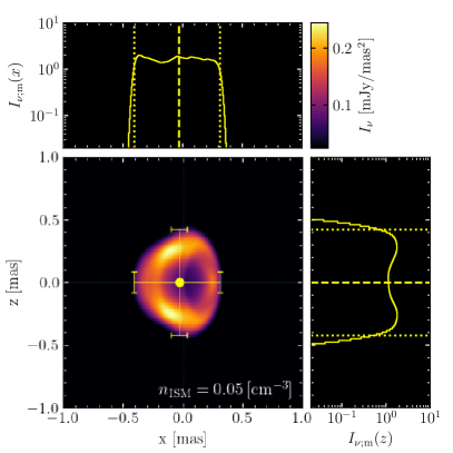
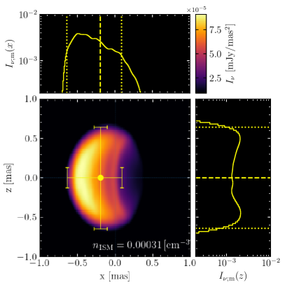
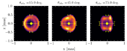
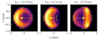
Figure 1: Top figure: sky map for a BNS merger simulation with BLh EOS and $q=1.00$ computed at $120\,$ days after the merger at $\nu=1\,$GHz and observed at $\theta_{\rm obs}=45\,$deg. Left and right columns of plots corresponds to different ISM densities, $n_{\rm ISM}=0.05\,\,\text{cm}^{-3}$ on the left and $n_{\rm ISM}=0.00031\,\,\text{cm}^{-3}$ on the right. In each plot column, the top and top-right subplots display the $X$ and $Z$ averaged brightness distributions respectively. Dotted lines mark FWHM and dashed lines mark the location of the flux centroid of the image. FWHM and the location of the flux centroid are also shown on the main panel of the figure as error bars and the circular marker respectively. Thin gray dotted lines indicate the $X$ and $Z$ axis. Notably, we are plotting $I_{\nu}/I_{\nu;\,\rm max}\in(0.1,1)$ range of the normalized specific intensity in order to resolve the image structure more clearly. Bottom panel: same sky map but viewed at three difference angles, $\theta_{\rm obs}$.

2 Methods

In order to compute the GRB and kN afterglows, we employ the semi-analytic code PyBlastAfterglow discussed in N22a and N21. In the model, both ejecta types are discretized into velocity and angular elements, for each of which the equations of BW evolution are solved independently, and the synchrotron radiation is computed, accounting for relativistic and time-of-arrival effects. The effect of the pre-processing of ISM medium by a passing GRB BW is considered in Sec. 3.3, otherwise this effect is not included, and kN BWs evolved independently from the GRB BWs. For kN afterglow, both thermal and non-thermal electron populations are considered, while for GRB afterglow only the latter is employed in the model.

The sky maps are computed using the spherical coordinate system discussed in Sec. $2$ in N22a (figure 1). For both ejecta types axial symmetry is assumed. Then, each elemental BW has radial coordinate $R_{ij}$, and angular coordinates $\theta_{i}$ and $\phi_{ij}$, where the single index of $\theta_{i}$ reflects the axial symmetry. The coordinate vector of the elemental BW is given by $\vec{v}_{ij}=R_{ij}\big{(}\sin{(\theta_{i})}\cos{(\phi_{ij})}\vec{x},\,\sin{(\theta_{i})}\sin{(\phi_{ij})}\vec{y},\,\cos{(\theta_{i})}\vec{z}\big{)}$. The cosine of the angle between the LOS and $\vec{v}_{ij}$ reads,

$$\mu_{ij}=\sin{(\theta_{i})}\sin{(\phi_{ij})}\sin(\theta_{\rm obs})+\cos{(\theta_{i})}\cos(\theta_{\rm obs})\,.$$ (1)

The image plane, $xz$ is perpendicular to the LOS of the observer. We chose the basis with which the principal jet moves in the positive $\tilde{x}$-direction. The basis vectors then $\tilde{\vec{x}}_{ij}=\sin(\theta_{\rm obs})\vec{z}_{ij}-\cos(\theta_{\rm obs})\vec{x}_{ij}$, $\tilde{\vec{y}}_{ij}=\vec{x}_{ij}$ of the plane as in Fernández et al. (2021) and the coordinates of the $ij$ BW on the image plane (for the principle jet) are given by

$$\tilde{x}_{ij} =-R_{ij}[\cos(\theta_{\rm obs})\sin(\theta_{i})\sin(\phi_{ij})$$ (2)

$$+\sin(\theta_{\rm obs})\cos(\theta_{i}))],$$

$$\tilde{z}_{ij} =R_{ij}\sin(\theta_{i})\cos(\phi_{ij})\,.$$

In the following, we omit the use of tildas for simplicity.

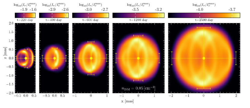
Figure 2: Evolution of the sky map for the BNS merger simulation with BLh EOS and $q=1.00$, observed at $\theta_{\rm obs}=45\,$deg, $\nu_{\rm obs}=1\,$GHz. The ISM density is $n_{\rm ISM}=0.05\,\,\text{cm}^{-3}$. As in Fig. 1, the marker and the error bar indicate the location of the flux centroid and the FWHM of the image, while gray dotted lines mark the axis.

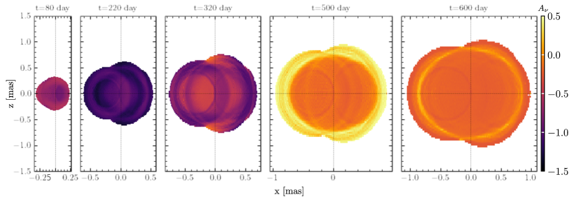
Figure 3: Evolution of the sky map spectral index for the BNS merger simulation with BLh EOS and $q=1.00$, observed at $\theta_{\rm obs}=45\,$deg. and at $\nu=1\,$GHz. Here $n_{\rm ISM}=0.05\,\,\text{cm}^{-3}$. Thin dotted lines mark the axis. For clarity, we did not apply the Gaussian smoothing kernel to this image.

In order to characterize sky maps we consider the following main quantities. Specifically, following Zrake et al. (2018); Fernández et al. (2021) we compute the surface brightness-weighted center of the image, image centroid, defined as

$$x_{c}=\frac{1}{\int I_{\nu}dxdz}\int xI_{\nu}dxdz,$$ (3)

where $I_{\nu}$ is computed via Eq. (37) in N22a. We also compute the $X$ and $Z$-averaged brightness distributions

$$I_{\nu;\rm m}(x) =\frac{1}{\Delta z}\int I_{\nu}(x,z)dz\,,$$ (4)

$$I_{\nu;\rm m}(z) =\frac{1}{\Delta x}\int I_{\nu}(x,z)dx\,.$$

As the available ejecta profiles are limited in the angular resolution, which severely limits the accuracy of the sky map analysis, we “rebin” the angular ejecta distribution histograms. To do this rebinning we assume a uniform distribution within each bin Knoll (2000).

3 Results

For an extended source with uniform Lorentz factor (LF) $\Gamma$, the maximal apparent velocity $\beta_{\rm app}<\Gamma$, while the image size increases with $\Gamma$ Boutelier et al. (2011). A spherically symmetric source that expands isotropically, would appear as a ring expanding with $\Gamma$ with no motion in the image centroid.

Due to non-trivial ejecta angular and velocity structure a kN sky map shape, size and structure have a complex dependency on the observer time $t_{\rm obs}$ and angle $\theta_{\rm obs}$. Moreover, if both, thermal and non-thermal electron populations are present behind the shock, there is a non-trivial dependency on the microphysical parameters and ISM density. It is beyond the scope of this work to study all possible combinations of free parameters. Instead, we focus on several representative cases.

Specifically, we fix the source to be located at luminosity distance, $D_{L}=41.3\,$Mpc with redshift $Z=0.0099$. The micropthysics parameters are the following. Fractions of the shock energy that goes into electron acceleration and magnetic field amplification are $\epsilon_{e}=0.1$, $\epsilon_{b}=0.001$, $\epsilon_{t}=1$. The slope of the power-law electron distribution is $p=2.05$. Unless stated otherwise, the observational frequency is $1\,$GHz., and the observer angle is $45\,$deg. We focus on two $n_{\rm ISM}$: the fiducial value $n_{\rm ISM}=0.05\,\,\text{cm}^{-3}$ and the value inferred for GRB170817A, $n_{\rm ISM}=0.00031\,\,\text{cm}^{-3}$.

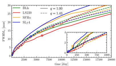
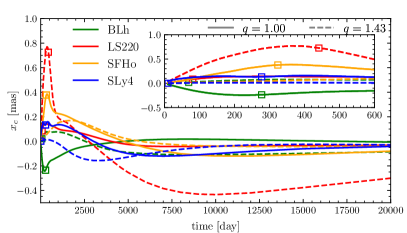
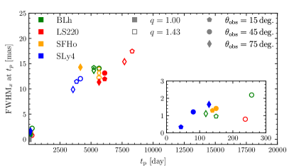
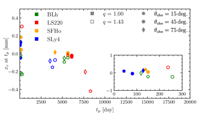
Figure 4: Time evolution of kN afterglow sky map properties. Top left panel shows the evolution of the image size, FWHM_x Circular markers indicate the image size at the LC peak. Top right panel shows the evolution of the flux centroid, $x_{c}$ position. Square markers indicate the minimum of the LC spectral index $A_{\nu}$. Bottom left panel and Bottom right panel display the image size and the position of the flux centroid at the time of the LC peak respectively for three values of the observational angle. In each panel there is a subpanel, enlarging an early-time part of the plot. Here $n_{\rm ISM}=0.00031\,\,\text{cm}^{-3}$.

3.1 Kilonova afterglow sky maps

We begin by considering the BNS merger simulation with BLh EOS and $q=1.00$. The sky map for $\theta_{\rm obs}=45\,$deg, $\nu_{\rm obs}=1\,$GHz and $t_{\rm obs}=120\,$days after merger is shown in Fig. 1.

At $t_{\rm obs}=120\,$days the kN afterglow at $1\,$GHz for this BNS merger model is dominated by the emission from thermal electron population behind shocks. The fast tail of the dynamical ejecta in this simulation is predominantly equatorial, confined to ${\gtrsim}60\,$deg (see Fig. 3 in N21) with mass-averaged half- root mean square (RMS) angle $\theta_{\rm RMS}\simeq 70\,$deg. As $\theta_{\rm RMS}>\theta_{\rm obs}$, the synthetic image resembles a wheel with the brightest parts offset from the center into the negative half of the $x$ axis, i.e., $x_{c}<0$. (See $\theta_{\rm obs}=15\,$deg. and $\theta_{\rm obs}=45\,$deg. subpanels in Fig. 1). An observer with $\theta_{\rm obs}\gtrsim\theta_{\rm RMS}$ would, however, be able to see the beamed emission from the fast ejecta tail (bright spots at $x\simeq 0\,$mas, $z\simeq\pm 0.3\,$mas on $\theta_{\rm obs}=75\,$deg. sub-panels of Fig. 1). Correspondingly, the image flux centroid lies near $x_{c}\simeq 0$ and the brightest part of the image laying in $x>0$ plane.

As the kN BWs propagates through the ISM, the size of a sky map increases in both $x$ and $z$ directions. Due to the axial symmetry of the ejecta properties, $\theta_{\rm obs}$ and relativistic effects primarily affect the FWHM_x and $x_{c}$. The example of a sky map evolution is shown in Fig. 2. Deceleration of kN BWs reduces the contribution from thermal electron population to the observed flux. Additionally, relativistic effects become increasingly less important. Consequently, the image becomes more spherically symmetric and centered around $x_{c}=z_{c}=0$. Specifically for this simulation, at $t_{\rm obs}=600\,$days after the merger the emission from equatorial and polar BWs becomes comparable with each other and thereafter the sky map resembles a circle with two bright spots near the image’s outer boundaries on the $x=0$ axis. These spots mark the geometrically overlapping emitting areas and reflect the equatorial nature of the ejecta fast tail. Notably, the presence of thermal electrons that we assume in our model does not affect this qualitative picture, as the emissivity from both thermal and non-thermal electron populations depend on the shock velocity albeit to a different degree (e.g. Ozel et al., 2000; Margalit & Quataert, 2021).

The presence of two electron populations behind BW shocks, however, implies a spectral evolution of the emission in every pixel of the sky map. We define a sky map spectral index as $A_{\nu}=d\log_{10}(I_{\nu})/d\log_{10}(\nu)$ and show its evolution in Fig. 3 for $\theta_{\rm obs}=45\,$deg. and $\nu=1\,$GHz. At early times, most of the sky map displays relatively low $A_{\nu}\simeq-1.25$, indicative of the emission from thermal electron populations (figure 3 in N22a). As the BWs decelerate and emission from the thermal electron population subsides. At the point where the spectrum transitions, the spectral index reaches a minimum. After that, the spectral index rises as the sky map becomes increasingly dominated by emission from the non-thermal electron population. At very late times the spectral map becomes uniform, as the emission from power-law electrons with fixed distribution slope $p$ dominates in every pixel. If resolved in observations, such evolution of the spectral sky map would allow a detailed study of the ejecta velocity and angular distribution, besides constraining the physics of particle acceleration at mildly relativistic shocks.

It is interesting to examine the evolution of the key sky map properties, image size FWHM_x, and the position of the flux centroid, $x_{c}$, at very low ISM density, that was generally inferred for GRB170817A. In Fig. 4, we show the evolution of the FWHM_x and $x_{c}$ as well as these values at the peak time $t_{p}$ of the respective LCs. The sky map size at a given epoch is primarily determined by the energy budget of the ejecta. Simulations with $q=1$ and soft EOS, e.g., SFHo and SLy4 EOSs display larger image sizes throughout the evolution. On the other hand, equal mass simulations with stiffer EOS, such as BLh and LS220 EOSs demonstrate smaller image sizes, More asymmetric binaries display in general intermediate image sizes.

At the time of the LC peak, the image size depends on whether the emission from thermal or non-thermal electron population dominates the observed flux. If former is true, $t_{p}$ is generally small, $t_{p}<500\,$ days for our simulations and assumed $n_{\rm ISM}=0.00031\,\,\text{cm}^{-3}$, and the image size case does not exceed $4\,$mas. Notably, at higher $n_{\rm ISM}$ $t_{p}$ is shorter and thus, the FWHM_x is smaller. Simulations with $q=1.00$ and soft (SLy4 and SFHo) EOSs are examples of that. If the emission from power-law electrons dominates the observed flux at the time of the LC peak, the image size is significantly larger, ${\simeq}15-20\,$mas. Importantly, $t_{p}$ depends also on the observer angle $\theta_{\rm obs}$ due to relativistic beaming of the early-time emission from thermal electrons. For example, a simulation with a sufficiently spherically symmetric distribution of the fast tail, simulation with SLy4 EOS and $q=1.00$ display an early $t_{p}<500\,$days at all three observing angles considered.

A characteristic feature of the changing dominant contributor (e.g., electron population) to the observed emission is seen here as a sharp increase in the evolution of image size (sub-panel in the top left panel in Fig. 4). This rapid increase in FWHM_x occurs when the emission from fast BWs, dominating the observed flux at first, subsides and less beamed, more isotropic emission from non-thermal electrons becomes equally important.

As discussed before, the evolution of the image flux centroid position, $X_{c}$, besides the ejecta energy budget, depends strongly on the observational angle. At $\theta_{\rm obs}=45\,$deg. for BNS merger models with sufficiently fast and equatorial fast tail, $x_{c}$ is negative at an early time (e.g., for simulation with BLh EOS and $q=1.00$). For simulations with $\theta_{\rm RMS}<\theta_{\rm obs}$, $x_{c}$ moves into the positive half of $x$ axis at the beginning, as is the the case for the equal mass simulations with SFHo, SLy4 and LS220 EOSs. The time evolution of the $x_{c}$ in most cases exhibits an extremum after which $x_{c}\rightarrow 0$. We find that the time of the extremum corresponds to the time where the spectral index evolution of the LC reaches minimum (see figure $4$ in N22a for the LC spectral index evolution). In the top right panel of Fig. 4 this point is shown with square marker.

At the time of the LC peak the position of the flux centroid is generally determined by whether the thermal or non-thermal electrons dominate the observed flux. This in turn depends on $\theta_{\rm obs}$. In the former case $|x_{c}|$ tends to be larger, reaching $|x_{c}|\leq 0.5\,$mas, as bright beamed emission from thermal electrons in fast BWs makes the image very asymmetric. Consequently, if the LC peaks at late times, $|x_{c}|$ is closer to zero for most models.

3.2 kN and GRB skymaps

One of the key observables of GRB170817A that confirmed the jetted nature of the outflow and allowed for a more precise estimate of the inclination angle $\theta_{\rm obs}$, was the motion of the GRB flux centroid Mooley et al. (2018a). Here we investigate, how the presence of the kN afterglow affects the GRB afterglow sky map $x_{c}$ and FWHM_x assuming that these two ejecta types do not interact. We briefly remark on this interaction in Sec. 3.3.

For modeling GRB afterglows, we consider the same parameters as in N22a, motivated by the analysis of GRB170817A (e.g. Hajela et al., 2019; Fernández et al., 2021), varying only the observer angle, $\theta_{\rm obs}$ and the ISM density $n_{\rm ISM}$. Specifically, we set the jet half-opening angle $\theta_{\rm w}=15\,$deg. and core half-opening angle $\theta_{\rm c}=4.9\,$deg. The isotropic equivalent energy is $E_{\rm iso}=10^{52}\,$ergs, and the initial LF of the core is $\Gamma_{\rm c}=300$. The microphysical parameters are set as: $\epsilon_{e}=0.05$, $\epsilon_{B}=0.0045$, and $p=2.16$. Luminosity distance to the source is set to $D_{\rm L}=41.3\,$Mpc. Unless stated otherwise, we consider $\theta_{\rm obs}=45\,$deg., and $n_{\rm ISM}=0.00031\,\,\text{cm}^{-3}$, as fiducial values.

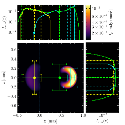
Figure 5: Combined kN and GRB sky map. The former can be seen as a dim blob on the left, while the latter – as a bright crescent on the right. The size and the location of the flux centroid of two individual components are shown with yellow and cyan colors respectively. The size and $X_{c}$ of the combined image are shown as lime color. As in Fig. 1 the top and right sub-panels display the $z$- and $x$-averaged brightness distributions respectively. Sky map corresponds to $\nu_{\rm obs}=1\,$GHz, $\theta_{\rm obs}=45\,$deg and $t_{\rm obs}=60\,$days, $n_{\rm ISM}=0.00031\,\,\text{cm}^{-3}$.

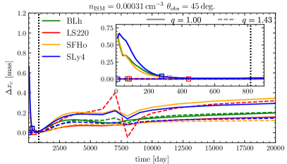
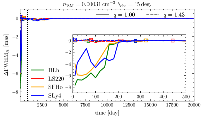
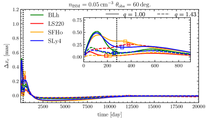
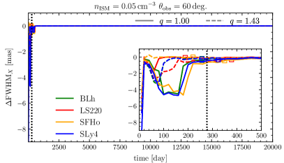
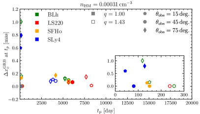
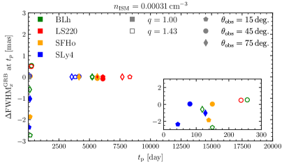
Figure 6: Top panels: time evolution of the combined sky map properties shown in terms of the $\Delta x_{c}^{\rm GRB}=(x_{c}^{\rm GRB}-x_{c}^{\rm kN})/x_{c}^{\rm GRB}$, $\Delta\text{FWHM}_{x}^{\rm GRB}=\text{FWHM}_{x}^{\rm GRB}-\text{FWHM}_{x}^{\rm kN}$ on the left and right panels respectively. Dashed gray line corresponds to the time of the GRB LC peak. Bottom panels: properties of the combined sky map extracted at the time of the kN afterglow LC peak. Different colors correspond to various EOSs. Filled and empty markers indicate $q=1.00$ and $q=1.43$ simulations respectively. Different markers correspond to various observing angles. In all panels, an inner sub-panel serves to enlarge the early time part of the figure.

In Fig. 5, we show a combined kN plus GRB afterglow radio sky map assuming $\theta_{\rm obs}=45\,$deg. and $t_{\rm obs}=60\,$days. At this early time the GRB afterglow is significantly brighter than the kN one: $F_{\nu=1\,{\rm GHz}}^{\rm GRB}=7.5\times 10^{-3}\,$mJy and $F_{\nu=1\,{\rm GHz}}^{\rm kN}=4\times 10^{-4}\,$mJy. However, despite being dimmer, kN afterglow affects the properties of the total sky map significantly, shifting the position of the image flux centroid back to the center of the explosion. Consequently, the apparent velocity computed from the motion of the flux centroid would be underestimated if the effect of kN afterglow is not taken into account. In our case, the apparent velocity is reduced from $2.5\,c$ to $2.1\,c$ at $t_{\rm obs}=60\,$days. Thus systematic underestimation of the apparent velocity may, in turn, result in overestimation of the $\theta_{\rm obs}$ or $\Gamma$. This can be understood from the following considerations. Consider, $(\theta_{\rm s}\leq\theta_{\rm obs}-\theta_{\rm s})$, where $\theta_{s}$ is the average size of the extended source. There, the maximum apparent velocity $\beta_{\rm app}$ is equal to the source LF $\Gamma$, as $\theta_{\rm obs}=1/\Gamma$. Then, assuming that the observed emission from an extended source comes predominantly from the compact region we have, $(\theta_{\rm obs}-\theta_{\rm s})\approxeq 1/\beta_{\rm app}$. These arguments were used to infer $\Gamma$ from radio image for GRB170817A Mooley et al. (2018a).

Notably, at smaller observational angles, the early GRB afterglow is significantly brighter, and at $\theta_{\rm obs}\simeq 20\,$deg. that is generally inferred for GRB170817A, the kN afterglow does not affect the estimated $\beta_{\rm app}$ to an appreciable degree.

At slightly later times, when the GRB afterglow reaches its peak emission we find that even for $\theta_{\rm obs}=45\,$deg, the effect of the kN afterglow on the GRB afterglow sky map properties is negligible. At the time of the GRB LC peak $t_{\rm p}^{\rm GRB}=800\,$days, the $\beta_{\rm app}$ is reduced only by ${\simeq}0.1\,c$.

The kN afterglow becomes important again later, when the GRB afterglow emission subsides. Numerical and semi-analytic jet models show, that both prime and counter jets contribute to the late time flux Zrake et al. (2018); Fernández et al. (2021). This forces the position of the flux centroid to move back to $x_{c}^{\rm GRB}\rightarrow 0$. Before that, the jet deceleration reduces the contribution to the observed emission from the fast jet core and consequently slows down the motion of the flux centroid. The jet lateral spreading contributes to this by pushing parts of the jet to $\theta>\theta_{\rm obs}$, making them move back on the image plane. In this regard, the presence of a kN afterglow might be confused with a more rapid lateral spreading or earlier emergence of the counter jet. Thus, we conclude that even if the kN afterglow does not contribute significantly to the observed total flux, it should be taken into account for accurate estimation of the jet energy and geometry from sky map observations. Importantly, the relative brightness of two afterglows considered here depends on all free parameters of the model i.e., microphysics parameters of both shock types (relativistic and mildly relativistic) as well as the angular and velocity structure of ejecta.

Considering the available BNS merger simulations, we recall that the kN afterglow from $q=1$ and soft EOSs simulations is brighter, and thus it would affect the properties of the combined sky map more strongly, at least before the GRB LC peak $t_{\rm p}^{\rm GRB}$. In Fig. 6, we show the change in GRB afterglow $x_{c}^{\rm GRB}$ and FWHM_x in terms of $\Delta v=(v^{\rm GRB}-v^{\rm kN})/v^{\rm GRB}$, where $v\in[x_{c},\text{FWHM${}_{x}${}}]$. As expected, the general effect of the inclusion of the kN afterglow is the decrease in $X_{c}$ and, consequently, in the apparent velocity $\beta_{\rm app}$, and an increase in the image FWHM_x (top right and left panels of Fig. 6). Specifically, $\Delta x_{c}$ and $\Delta$FWHM_x reach ${\gtrsim}0.5$ and ${\gtrsim}-8$ respectively.

At $t_{\rm p}^{\rm GRB}$ the effect of the kN afterglow presence is minimal in all cases, as the GRB afterglow dominates the total emission and the sky map properties. Thus, estimated at this time, image properties convey the most reliable information about the GRB afterglow.

At higher $n_{\rm ISM}$ and $\theta_{\rm obs}$, the picture is qualitatively similar. Influence of the kN afterglow is the most prominent at $t<t_{\rm p}^{\rm GRB}$ and for equal mass BNS simulations with soft EOS, such as SLy4 and SFHo EOSs. For $q>1$ simulations, the maximum $\Delta x_{c}$ and $\Delta$FWHM_x are about two times smaller than in $q=1$ cases. On the other hand, at $\theta_{\rm obs}=21.5\,$deg., and $n_{\rm ISM}=0.00031\,\,\text{cm}^{-3}$, the influence of the kN afterglow is negligible even at $t<t_{\rm p}^{\rm GRB}$ for all simulations. In this case GRB afterglow provides a dominant contribution to the total LC and the sky map, and the presence of kN afterglow can only be seen at very late times $t\gg t_{\rm p}^{\rm GRB}$, when the kN afterglow emission is coming predominantly from the non-thermal electron population. Meanwhile, in cases when the early GRB emission is beamed away, $\theta_{\rm obs}\gtrsim 45\,$deg, the maximum in $\Delta x_{c}$ and $\Delta$FWHM_x occurs before the extreme in kN afterglow spectral index evolution, in the regime where the emission from thermal electrons dominate the observed flux.

3.3 Effect of the GRB-modified ISM on kN afterglow sky map

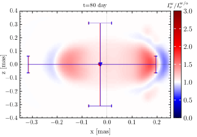
Figure 7: The ratio between two kN afterglow sky maps with the only difference between them being is whether the CBM, altered by a passage of GRB BWs, is taken into account ($I_{\nu}^{\rm w}$) or not ($I_{\nu}^{w/o}$). Image size and the position of the flux centroid are shown as before with error bars and markers with blue color for “w” case and red for “w/o” case. Sky maps are computed assuming $\nu_{\rm obs}=1\,$GHz, $\theta_{\rm obs}=60\,$deg., and $n_{\rm ISM}=0.05\,\,\text{cm}^{-3}$.

In N22a we showed that when the kN ejecta moves behind the GRB BW, it encounters an altered density profile, that we called an altered CBM, and the afterglow signature changes. Specifically, the observed flux first decreases as most of the kN ejecta moves subsonically behind the laterally spreading GRB BW, then increases as the kN ejecta shocks the overdense fluid behind the GRB BW forward shock. However, the decrease and increase in the observed flux were found to be rather small: $\lesssim 40\%$ and $\lesssim 10\%$, respectively. The reason for this is the non-uniform nature of the kN ejecta and finite time that GRB lateral spreading takes. Thus, different parts of the kN ejecta encounter different regions of the altered CBM at a given time producing either an excess or a reduction in observed emission. Nevertheless, for the sake of completeness, it is worth looking at how the kN afterglow sky map changes the altered CBM is taken into account.

In Fig. 7 we show the effect of an altered CBM on the kN afterglow sky map for $t_{\rm obs}=80\,$days, $\theta_{\rm obs}=60\,$deg., and $n_{\rm ISM}=0.05\,\,\text{cm}^{-3}$. The red and blue colors indicate the excess and the reduction of the observed emission with respect to the sky map computed when the altered CBM is not taken into account. As expected, the change in the observed intensity occurs primarily near poles ($z=0$) and corresponds to kN ejecta moving subsonically and not producing synchrotron emission. Fast elements of the kN ejecta shocked the overdense region behind the GRB shock and produced an emission excess. Slower elements of ejecta catch up with the underdense part of the altered CBM later and this the part of the image where the emission is suppressed lies ahead of the one with emission excess. The more equatorial part of the ejecta avoids interacting with the altered CBM and, thus, its emission remains unchanged (along $z$ axis). The certain parts of the image, the emission excess can be significant, ($I_{\nu}^{\rm w}/I_{\nu}^{\rm w/o}\lesssim 3$). However, combined with the emission suppression in other parts of the image, the overall emission excess is rather small. Thus, even at this relatively high $n_{\rm ISM}$ and large $\theta_{\rm obs}$ the effect of the altered CBM on the sky map properties, i.e., the position of the flux centroid and the image size are negligible.

4 Discussion and conclusion

In this work, we considered synthetic radio images of the GRB and kN afterglow. For the former we considered GRB170817A motivated model settings, i.e., laterally structured jet observed off-axis Hajela et al. (2019); Fernández et al. (2021). For the latter, we considered a set of ejecta profiles from NR BNS merger simulations targeted to GW170817, i.e., with corresponding chirp mass. For all calculations, we use the semi-analytic afterglow code PyBlastAfterglow, presented and discussed in N21 and N22a. The key aspect of the input physics is the inclusion of two electron populations behind the kN BW shocks, that follow power-law (non-thermal electrons) and Maxwellian (thermal electrons) distributions.

The main limitation of our work is the semi-analytical nature of the model we employ. It remains to be investigated how GRB and kN afterglow sky maps computed with hydrodynamics (HD) numerical codes compare to ours. It is however numerically very challenging to perform such simulations on a temporal and spatial scales discussed in this work, as well as, to perform them for various possible choices of the model free parameters and kN ejecta profiles.

The aforementioned limitations notwithstanding, we find that the kN afterglow sky map at early times resemble a wheel or a doughnut due to the emission from thermal electrons enhanced by relativistic effects, dominating the observed flux. At later times, the sky map is largely spherical with a remaining ring structure reflecting the $a)$ assumed axial symmetry, $b)$ initial ejecta velocity distribution. The image size evolves monotonically, albeit not smoothly, reaching ${\simeq 10}\,$mas at $3000\,$days and ${\simeq}25\,$mas at $20000\,$days. If the kN afterglow LC at its peak is dominated by the emission from thermal electrons, the image size is smaller reaching ${\lesssim}5\,$mas. Thus, the properties of the fast ejecta tail can be inferred from the sky map size and its evolution.

Despite asymmetry in ejecta velocity distribution, however, the position of the image flux centroid $x_{c}$ does not deviate much from $0$, and is the largest ($|x_{c}|<0.4\,$mas) at early times, in cases when the emission from thermal electrons dominates the observed flux. Notably, however, the asymmetry can lead to the negative values of $|x_{c}|$ (assuming more on-axis observers), which if observed might hint at the equatorial nature of the fast ejecta tail.

Crucially, the presence of the kN ejecta can affect the GRB afterglow sky map to an appreciable degree even if the former does not appreciably contribute to the total observed flux. For that to occur, however, the source must be observed sufficiently off-axis so that the early GRB afterglow emission is beamed away, while the kN afterglow emission, dominated at this time by the emission from thermal electrons, is instead beamed more toward an observer. Specifically, at $t_{\rm obs}=80\,$days and assuming $\theta_{\rm obs}=45\,$deg. the change in the inferred value of the apparent velocity $\beta_{\rm app}$ can reach $0.5\,c$. At smaller $\theta_{\rm obs}$ the kN afterglow effects the GRB afterglow sky map properties significantly less and at $\theta_{\rm obs}\simeq 20\,$deg. we find the effect to be negligible. Importantly, the relative brightness between these two types of afterglow depends on their respective sets of free parameters that are largely unconstrained. It is thus important to conduct a more thorough statistical analysis of the combined parameter space to assess the upper and lower limits of the degree to which the kN afterglow influences the combined sky map properties.

The detectability of the kN and GRB sky maps with Next Generation Very Large Array (ngVLA), which is currently in the development will be discussed in a separate study by Eddins et. al. (2023, in prep.). Overall, in order for kN afterglow itself to be detectable, the flux density at the LC peak should be $\gtrsim 5\times 10^{-3}\,$mJy in radio Kathirgamaraju et al. (2019b). For BNS merger simulations considered here, this is only possible at sufficiently high density, $n_{\rm ISM}\gtrsim 0.005\,\,\text{cm}^{-3}$ at $D_{\rm L}\simeq 40\,$Mpc. In order to distinguish GRB and kN afterglows, the $\theta_{\rm obs}$ should be much larger than the jet opening angle (e.g., see figure 9 in N22a). At the same time, at large $\theta_{\rm obs}$ the change in the position of the sky map flux centroid due to the presence of the kN afterglow can become detectable. It is, however, difficult to determine what value of $x_{c}^{\rm GRB}-x_{c}^{\rm kN}$ can be resolved. At $n_{\rm ISM}=0.05\,\,\text{cm}^{-3}$ and $\theta_{\rm obs}=60\,$deg, the $x_{c}^{\rm GRB}-x_{c}^{\rm kN}$ reaches $0.5\,$mas for equal mass BNS models within the first $200\,$days after the burst which, in principle, should be detectable (Eddins et. al. (2023, in prep.)) with angular resolution of $0.1\,$mas.

Data Availability:

The datasets generated during and/or analyzed during the current study are available from the corresponding author on reasonable request.

References

- Abbott et al. (2017a) Abbott B. P., et al., 2017a, Phys. Rev. Lett., 119, 161101
- Abbott et al. (2017b) Abbott B. P., et al., 2017b, Astrophys. J. Lett., 848, L13
- Abbott et al. (2019a) Abbott B. P., et al., 2019a, Phys. Rev., X9, 011001
- Abbott et al. (2019b) Abbott B. P., et al., 2019b, Phys. Rev., X9, 031040
- Ajello et al. (2016) Ajello M., et al., 2016, Astrophys. J., 819, 44
- Alexander et al. (2017) Alexander K. D., et al., 2017, Astrophys. J., 848, L21
- Alexander et al. (2018) Alexander K., et al., 2018, Astrophys. J., 863, L18
- Arcavi et al. (2017) Arcavi I., et al., 2017, Nature, 551, 64
- Bauswein et al. (2013) Bauswein A., Goriely S., Janka H.-T., 2013, Astrophys.J., 773, 78
- Bernuzzi (2020) Bernuzzi S., 2020, Gen. Rel. Grav., 52, 108
- Bietenholz et al. (2014) Bietenholz M. F., De Colle F., Granot J., Bartel N., Soderberg A. M., 2014, Mon. Not. Roy. Astron. Soc., 440, 821
- Boutelier et al. (2011) Boutelier T., Henri G., Petrucci P. O., 2011, Mon. Not. R. Astron. Soc, 418, 1913
- Coughlin et al. (2019) Coughlin M. W., Dietrich T., Margalit B., Metzger B. D., 2019, Mon. Not. Roy. Astron. Soc., 489, L91
- Coulter et al. (2017) Coulter D. A., et al., 2017, Science, 358, 1556
- Cowperthwaite et al. (2017) Cowperthwaite P. S., et al., 2017, Astrophys. J., 848, L17
- Dalal et al. (2002) Dalal N., Griest K., Pruet J., 2002, Astrophys. J., 564, 209
- Desai et al. (2019) Desai D., Metzger B. D., Foucart F., 2019, Mon. Not. Roy. Astron. Soc., 485, 4404
- Dessart et al. (2009) Dessart L., Ott C., Burrows A., Rosswog S., Livne E., 2009, Astrophys.J., 690, 1681
- Dietrich & Ujevic (2017) Dietrich T., Ujevic M., 2017, Class. Quant. Grav., 34, 105014
- Dietrich et al. (2020) Dietrich T., Coughlin M. W., Pang P. T. H., Bulla M., Heinzel J., Issa L., Tews I., Antier S., 2020, Science, 370, 1450
- Drout et al. (2017) Drout M. R., et al., 2017, Science, 358, 1570
- Evans et al. (2017) Evans P. A., et al., 2017, Science, 358, 1565
- Fahlman & Fernández (2018) Fahlman S., Fernández R., 2018, Astrophys. J., 869, L3
- Fernández et al. (2015) Fernández R., Quataert E., Schwab J., Kasen D., Rosswog S., 2015, Mon. Not. Roy. Astron. Soc., 449, 390
- Fernández et al. (2019) Fernández R., Tchekhovskoy A., Quataert E., Foucart F., Kasen D., 2019, Mon. Not. Roy. Astron. Soc., 482, 3373
- Fernández et al. (2021) Fernández J. J., Kobayashi S., Lamb G. P., 2021, Mon. Not. Roy. Astron. Soc., 509, 395
- Fong et al. (2017) Fong W., et al., 2017, Astrophys. J. Lett., 848, L23
- Fujibayashi et al. (2018) Fujibayashi S., Kiuchi K., Nishimura N., Sekiguchi Y., Shibata M., 2018, Astrophys. J., 860, 64
- Fujibayashi et al. (2020) Fujibayashi S., Shibata M., Wanajo S., Kiuchi K., Kyutoku K., Sekiguchi Y., 2020, Phys. Rev. D, 101, 083029
- Fujibayashi et al. (2023) Fujibayashi S., Kiuchi K., Wanajo S., Kyutoku K., Sekiguchi Y., Shibata M., 2023, Astrophys. J., 942, 39
- Gal-Yam et al. (2006) Gal-Yam A., et al., 2006, Astrophys. J., 639, 331
- Ghirlanda et al. (2019) Ghirlanda G., et al., 2019, Science, 363, 968
- Gill & Granot (2018) Gill R., Granot J., 2018, Mon. Not. Roy. Astron. Soc., 478, 4128
- Granot et al. (2001) Granot J., Miller M. A., Piran T., Suen W.-M., Hughes P. A., 2001, ] 10.1007/10853853 82
- Granot et al. (2002) Granot J., Panaitescu A., Kumar P., Woosley S. E., 2002, Astrophys. J. Lett., 570, L61
- Granot et al. (2004) Granot J., Ramirez-Ruiz E., Loeb A., 2004, Astrophys. J., 618, 413
- Hajela et al. (2019) Hajela A., et al., 2019, Astrophys. J. Lett., 886, L17
- Hajela et al. (2022) Hajela A., et al., 2022, Astrophys. J. Lett., 927, L17
- Hallinan et al. (2017) Hallinan G., et al., 2017, Science, 358, 1579
- Harris et al. (2020) Harris C. R., et al., 2020, Nature, 585, 357
- Hotokezaka & Piran (2015) Hotokezaka K., Piran T., 2015, Mon. Not. Roy. Astron. Soc., 450, 1430
- Hotokezaka et al. (2013a) Hotokezaka K., Kiuchi K., Kyutoku K., Muranushi T., Sekiguchi Y.-i., Shibata M., Taniguchi K., 2013a, Phys. Rev. D, 88, 044026
- Hotokezaka et al. (2013b) Hotokezaka K., Kiuchi K., Kyutoku K., Okawa H., Sekiguchi Y.-i., Shibata M., Taniguchi K., 2013b, Physical Review D, 87.2, 024001
- Hotokezaka et al. (2018) Hotokezaka K., Kiuchi K., Shibata M., Nakar E., Piran T., 2018, Astrophys. J., 867, 95
- Huang et al. (2020) Huang Y.-J., et al., 2020, Astrophys. J., 897, 69
- Hunter (2007) Hunter J. D., 2007, Computing in Science & Engineering, 9, 90
- Just et al. (2015) Just O., Bauswein A., Pulpillo R. A., Goriely S., Janka H. T., 2015, Mon. Not. Roy. Astron. Soc., 448, 541
- Kasen et al. (2013) Kasen D., Badnell N. R., Barnes J., 2013, Astrophys. J., 774, 25
- Kasen et al. (2015) Kasen D., Fernández R., Metzger B., 2015, Mon. Not. Roy. Astron. Soc., 450, 1777
- Kasliwal et al. (2017) Kasliwal M. M., et al., 2017, Science, 358, 1559
- Kathirgamaraju et al. (2019a) Kathirgamaraju A., Tchekhovskoy A., Giannios D., Barniol Duran R., 2019a, Mon. Not. Roy. Astron. Soc., 484, L98
- Kathirgamaraju et al. (2019b) Kathirgamaraju A., Giannios D., Beniamini P., 2019b, Mon. Not. Roy. Astron. Soc., 487, 3914
- Kawaguchi et al. (2018) Kawaguchi K., Shibata M., Tanaka M., 2018, Astrophys. J., 865, L21
- Knoll (2000) Knoll G. F., 2000, Radiation Detection and Measurement, 3rd ed., 3rd edition edn. John Wiley and Sons, New York
- Krüger & Foucart (2020) Krüger C. J., Foucart F., 2020, Phys. Rev. D, 101, 103002
- Kulkarni (2005) Kulkarni S., 2005
- Kumar & Panaitescu (2000) Kumar P., Panaitescu A., 2000, Astrophys. J. Lett., 541, L51
- Lamb & Kobayashi (2017) Lamb G. P., Kobayashi S., 2017, Mon. Not. Roy. Astron. Soc., 472, 4953
- Lamb et al. (2018) Lamb G. P., Mandel I., Resmi L., 2018, Mon. Not. Roy. Astron. Soc., 481, 2581
- Lattimer & Schramm (1974) Lattimer J. M., Schramm D. N., 1974, Astrophys. J., 192, L145
- Levinson et al. (2002) Levinson A., Ofek E., Waxman E., Gal-Yam A., 2002, Astrophys. J., 576, 923
- Li & Paczynski (1998) Li L.-X., Paczynski B., 1998, Astrophys. J. Lett., 507, L59
- Lyman et al. (2018) Lyman J. D., et al., 2018, Nat. Astron., 2, 751
- Margalit & Quataert (2021) Margalit B., Quataert E., 2021, Astrophys. J. Lett., 923, L14
- Margutti et al. (2018) Margutti R., et al., 2018, Astrophys. J., 856, L18
- Martin et al. (2015) Martin D., Perego A., Arcones A., Thielemann F.-K., Korobkin O., Rosswog S., 2015, Astrophys. J., 813, 2
- Mesler & Pihlström (2013) Mesler R. A., Pihlström Y. M., 2013, Astrophys. J., 774, 77
- Mesler et al. (2012) Mesler R. A., Pihlström Y. M., Taylor G. B., Granot J., 2012, Astrophys. J., 759, 4
- Metzger (2020) Metzger B. D., 2020, Living Rev. Rel., 23, 1
- Metzger & Fernández (2014) Metzger B. D., Fernández R., 2014, Mon.Not.Roy.Astron.Soc., 441, 3444
- Metzger et al. (2010) Metzger B. D., et al., 2010, Monthly Notices of the Royal Astronomical Society, 406, 2650
- Metzger et al. (2015) Metzger B. D., Bauswein A., Goriely S., Kasen D., 2015, Mon. Not. Roy. Astron. Soc., 446, 1115
- Metzger et al. (2018) Metzger B. D., Thompson T. A., Quataert E., 2018, Astrophys. J., 856, 101
- Miller et al. (2019) Miller J. M., et al., 2019, Phys. Rev., D100, 023008
- Moderski et al. (2000) Moderski R., Sikora M., Bulik T., 2000, Astrophys. J., 529, 151
- Mooley et al. (2018a) Mooley K. P., et al., 2018a, Nature, 561, 355
- Mooley et al. (2018b) Mooley K. P., et al., 2018b, Astrophys. J. Lett., 868, L11
- Mooley et al. (2022) Mooley K. P., Anderson J., Lu W., 2022, Nature, 610, 273
- Nakar (2020) Nakar E., 2020, Phys. Rept., 886, 1
- Nakar & Piran (2003) Nakar E., Piran T., 2003, New Astron., 8, 141
- Nakar & Piran (2011) Nakar E., Piran T., 2011, Nature, 478, 82
- Nakar & Piran (2021) Nakar E., Piran T., 2021, Astrophys. J., 909, 114
- Nakar et al. (2002) Nakar E., Piran T., Granot J., 2002, Astrophys. J., 579, 699
- Nathanail et al. (2021) Nathanail A., Gill R., Porth O., Fromm C. M., Rezzolla L., 2021, Mon. Not. Roy. Astron. Soc., 502, 1843
- Nedora et al. (2019) Nedora V., Bernuzzi S., Radice D., Perego A., Endrizzi A., Ortiz N., 2019, Astrophys. J., 886, L30
- Nedora et al. (2021a) Nedora V., Radice D., Bernuzzi S., Perego A., Daszuta B., Endrizzi A., Prakash A., Schianchi F., 2021a, Mon. Not. Roy. Astron. Soc., 506, 5908
- Nedora et al. (2021b) Nedora V., et al., 2021b, Astrophys. J., 906, 98
- Nedora et al. (2022a) Nedora V., Dietrich T., Shibata M., Pohl M., Menegazzi L. C., 2022a, Mon. Not. Roy. Astron. Soc.
- Nedora et al. (2022b) Nedora V., et al., 2022b, Class. Quant. Grav., 39, 015008
- Nicholl et al. (2017) Nicholl M., et al., 2017, Astrophys. J., 848, L18
- Nynka et al. (2018) Nynka M., Ruan J. J., Haggard D., Evans P. A., 2018, Astrophys. J. Lett., 862, L19
- Ozel et al. (2000) Ozel F., Psaltis D., Narayan R., 2000, The Astrophysical Journal, 541, 234
- Panaitescu & Meszaros (1999) Panaitescu A., Meszaros P., 1999, Astrophys. J., 526, 707
- Perego et al. (2014) Perego A., Rosswog S., Cabezon R., Korobkin O., Kaeppeli R., et al., 2014, Mon.Not.Roy.Astron.Soc., 443, 3134
- Perego et al. (2017) Perego A., Radice D., Bernuzzi S., 2017, Astrophys. J., 850, L37
- Perego et al. (2019) Perego A., Bernuzzi S., Radice D., 2019, Eur. Phys. J., A55, 124
- Perna & Loeb (1998) Perna R., Loeb A., 1998, Astrophys. J. Lett., 509, L85
- Pihlstrom et al. (2007) Pihlstrom Y. M., Taylor G. B., Granot J., Doeleman S., 2007, Astrophys. J., 664, 411
- Piran et al. (2013) Piran T., Nakar E., Rosswog S., 2013, Mon. Not. Roy. Astron. Soc., 430, 2121
- Radice et al. (2016) Radice D., Galeazzi F., Lippuner J., Roberts L. F., Ott C. D., Rezzolla L., 2016, Mon. Not. Roy. Astron. Soc., 460, 3255
- Radice et al. (2018a) Radice D., Perego A., Hotokezaka K., Bernuzzi S., Fromm S. A., Roberts L. F., 2018a, Astrophys. J. Lett., 869, L35
- Radice et al. (2018b) Radice D., Perego A., Hotokezaka K., Fromm S. A., Bernuzzi S., Roberts L. F., 2018b, Astrophys. J., 869, 130
- Radice et al. (2020) Radice D., Bernuzzi S., Perego A., 2020, Ann. Rev. Nucl. Part. Sci., 70, 95
- Ramirez-Ruiz & Madau (2004) Ramirez-Ruiz E., Madau P., 2004, Astrophys. J. Lett., 608, L89
- Ramirez-Ruiz et al. (2005) Ramirez-Ruiz E., Granot J., Kouveliotou C., Woosley S. E., Patel S. K., Mazzali P. A., 2005, Astrophys. J. Lett., 625, L91
- Rau et al. (2006) Rau A., Greiner J., Schwarz R., 2006, Astronomy and Astrophysics, 449, 79
- Rhoads (1997) Rhoads J. E., 1997, Astrophys. J. Lett., 487, L1
- Rhoads (2003) Rhoads J. E., 2003, Astrophys. J., 591, 1097
- Roberts et al. (2011) Roberts L. F., Kasen D., Lee W. H., Ramirez-Ruiz E., 2011, The Astrophysical Journal Letters, 736, L21
- Rosswog (2005) Rosswog S., 2005, Astrophys. J., 634, 1202
- Rosswog et al. (1999) Rosswog S., Liebendoerfer M., Thielemann F., Davies M., Benz W., et al., 1999, Astron.Astrophys., 341, 499
- Ruan et al. (2018) Ruan J. J., Nynka M., Haggard D., Kalogera V., Evans P., 2018, Astrophys. J., 853, L4
- Ryan et al. (2020) Ryan G., van Eerten H., Piro L., Troja E., 2020, Astrophys. J., 896, 166
- Sari et al. (1999) Sari R., Piran T., Halpern J., 1999, Astrophys. J. Lett., 519, L17
- Savchenko et al. (2017) Savchenko V., et al., 2017, Astrophys. J. Lett., 848, L15
- Sekiguchi et al. (2015) Sekiguchi Y., Kiuchi K., Kyutoku K., Shibata M., 2015, Phys.Rev., D91, 064059
- Sekiguchi et al. (2016) Sekiguchi Y., Kiuchi K., Kyutoku K., Shibata M., Taniguchi K., 2016, Phys. Rev., D93, 124046
- Shibata & Hotokezaka (2019) Shibata M., Hotokezaka K., 2019, Ann. Rev. Nucl. Part. Sci., 69, 41
- Siegel & Metzger (2017) Siegel D. M., Metzger B. D., 2017, Phys. Rev. Lett., 119, 231102
- Smartt et al. (2017) Smartt S. J., et al., 2017, Nature, 551, 75
- Soares-Santos et al. (2017) Soares-Santos M., et al., 2017, Astrophys. J., 848, L16
- Soderberg et al. (2006) Soderberg A. M., Nakar E., Kulkarni S. R., 2006, Astrophys. J., 638, 930
- Tanaka & Hotokezaka (2013) Tanaka M., Hotokezaka K., 2013, Astrophys. J., 775, 113
- Tanaka et al. (2017) Tanaka M., et al., 2017, Publ. Astron. Soc. Jap., 69, psx12
- Tanvir et al. (2017) Tanvir N. R., et al., 2017, Astrophys. J., 848, L27
- Taylor et al. (2004) Taylor G. B., Frail D. A., Berger E., Kulkarni S. R., 2004, Astrophys. J. Lett., 609, L1
- Taylor et al. (2005) Taylor G. B., Momjian E., Pihlstrom Y., Ghosh T., Salter C., 2005, Astrophys. J., 622, 986
- Totani & Panaitescu (2002) Totani T., Panaitescu A., 2002, Astrophys. J., 576, 120
- Troja et al. (2017) Troja E., et al., 2017, Nature, 551, 71
- Villar et al. (2017) Villar V. A., et al., 2017, Astrophys. J., 851, L21
- Vincent et al. (2020) Vincent T., Foucart F., Duez M. D., Haas R., Kidder L. E., Pfeiffer H. P., Scheel M. A., 2020, Phys. Rev., D101, 044053
- Virtanen et al. (2020) Virtanen P., et al., 2020, Nature Methods, 17, 261
- Wanajo et al. (2014) Wanajo S., Sekiguchi Y., Nishimura N., Kiuchi K., Kyutoku K., Shibata M., 2014, Astrophys. J., 789, L39
- Winkler et al. (2011) Winkler C., Diehl R., Ubertini P., Wilms J., 2011, Space Science Reviews, 161, 149
- Woods & Loeb (1999) Woods E., Loeb A., 1999, Astrophys. J., 523, 187
- Wu et al. (2016) Wu M.-R., Fernández R., Martínez-Pinedo G., Metzger B. D., 2016, Mon. Not. Roy. Astron. Soc., 463, 2323
- Zappa et al. (2022) Zappa F., Bernuzzi S., Radice D., Perego A., 2022
- Zrake et al. (2018) Zrake J., Xie X., MacFadyen A., 2018, Astrophys. J. Lett., 865, L2