SplineCam: Exact Visualization and Characterization of Deep
Network Geometry and Decision Boundaries

Abstract

Current Deep Network (DN) visualization and interpretability methods rely heavily on data space visualizations such as scoring which dimensions of the data are responsible for their associated prediction or generating new data features or samples that best match a given DN unit or representation. In this paper, we go one step further by developing the first provably exact method for computing the geometry of a DN’s mapping – including its decision boundary – over a specified region of the data space. By leveraging the theory of Continuous Piece-Wise Linear (CPWL) spline DNs, SplineCam exactly computes a DN’s geometry without resorting to approximations such as sampling or architecture simplification. SplineCam applies to any DN architecture based on CPWL nonlinearities, including (leaky-)ReLU, absolute value, maxout, and max-pooling and can also be applied to regression DNs such as implicit neural representations. Beyond decision boundary visualization and characterization, SplineCam enables one to compare architectures, measure generalizability and sample from the decision boundary on or off the manifold. Project Website: bit.ly/splinecam.

1 Introduction

Deep learning and in particular Deep Networks (DNs) have redefined the landscape of machine learning and pattern recognition [23]. Although current DNs employ a variety of techniques that improve their performance, their core operation remains unchanged, primarily consisting of sequentially mapping an input vector $\bm{x}$ to a sequence of $L$ feature maps $\bm{z}^{\ell}$, $\ell=1,\dots,L$ by successively applying simple nonlinear transformations, called layers, as in

$$\bm{z}^{\ell}=\sigma\left(\bm{W}^{\ell}\bm{z}^{\ell-1}+\bm{b}^{\ell}\right),\quad\ell=1,\dots,L$$ (1)

starting with $\bm{z}^{0}=\bm{x}$, and denoting by $\bm{W}^{\ell}$ the weight matrix, $\bm{b}^{\ell}$ the bias vector, and $\sigma$ an activation operator that applies an element-wise nonlinear activation function. One popular choice for $\sigma$ is the Rectified Linear Unit (ReLU) [13] that takes the elementwise maximum between its entry and $0$. The parametrization of $\bm{W}^{\ell},\bm{b}^{\ell}$ controls the type of layer, e.g., circulant matrix for convolutional layer.

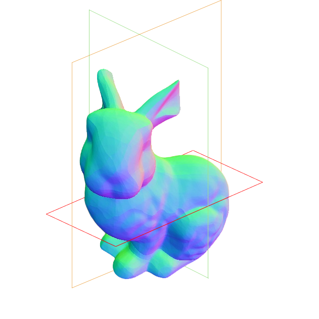
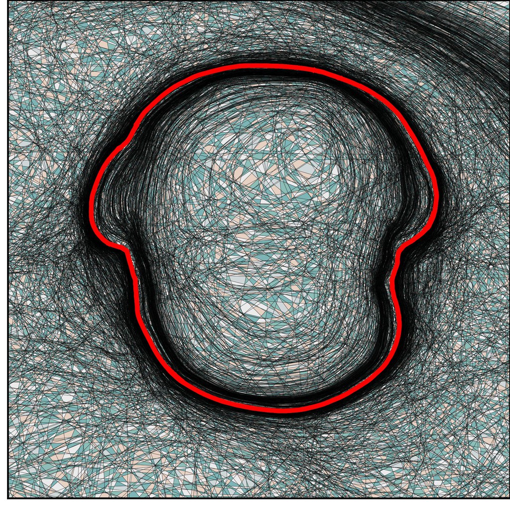
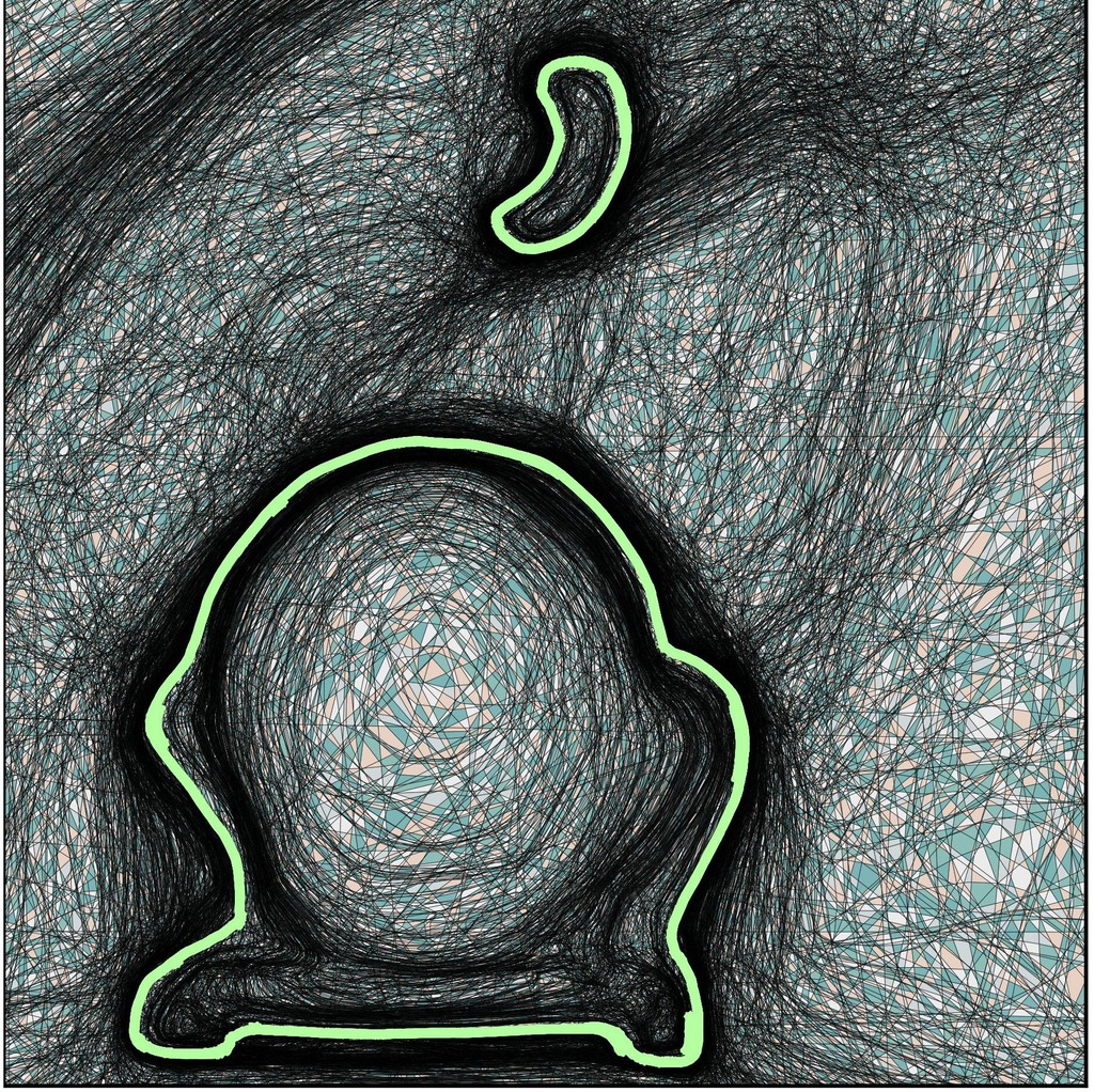
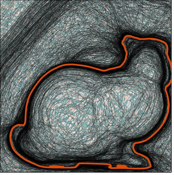
Figure 1: Exact visualization of the decision boundary and partition geometry of a 3D neural signed distance field (SDF). (Top left) Surface normals obtained from the learned signed distance field with annotations indicating slices used for visualization. For each of the slices, we can see the spline partition geometry of the learned SDF- each contiguous line represents a neuron, on either side of which it gets activated/deactivated. Neurons from different depths of the network create a partitioning of the input space into ’linear regions’. Here the colored lines represent the decision boundary learned by the SDF. Note that while the final neuron obtains the decision boundary, many neurons place their boundaries close to the ground truth surface to obtain the final SDF representation.

Interpreting the geometry of a DN is a nontrivial task since many different sets of parameters can lead to the same input-output mapping. One example is obtained by permuting the rows of $\bm{W}^{\ell},\bm{b}^{\ell}$ and the columns of $\bm{W}^{\ell+1}$ any two consecutive layers DN. Another example is to rescale $\bm{W}^{\ell},\bm{b}^{\ell}$ by some constant $\kappa$ and to rescale $\bm{W}^{\ell+1}$ by $1/\kappa$ for a ReLU-DN [33]; the list of such parameter manipulations preserving the underlying DN’s function is an active area of research [32]. Since one cannot trivially use the DN’s parameters to describe its mapping, practitioners have relied on different solutions to interpret what has been learned by a model by looking at the activations instead of the weights of the network [40, 20]. Activation based interpretability methods however can be susceptible to feature adversarial attacks, i.e., adversarial attacks that don’t cross the decision boundary but changes the activation [12]. An alternative empirical method for model interpretation is finding the closest point to a training sample $\bm{x}$ that lies on the model’s decision boundary [35]. Beyond interpretability, such methods find practical use in active learning [24] and adversarial robustness [16]. In this setting, one commonly performs gradient updates from an initial guess for $\bm{x}$ based on an objective function that reaches its minimum whenever its argument lies on the model’s decision boundary. While alternative and more efficient solutions have been developed, most of the progress in this direction has focused on providing more optimized losses and sampling strategies [35, 16]. In short, there doesn’t exist an exact (up to machine precision) method to compute the decision boundary of a DN.

In this paper, we focus on DNs employing Continuous Piece-Wise Linear (CPWL) activation functions $\sigma$, such as the (leaky-)ReLU, absolute value, and max-pooling. In this setting, the entire DN itself becomes a CPWL operator, i.e., its mapping is affine within regions of a partition of its domain. There has been previous studies dedicated to estimating the partition of such CPWL DNs and bridging empirical findings with interpretability. For example, Hanin et al. [14] connects the DN partition density with the complexity of the learned function, Jordan et al. [21] approximates the DN partition to provide robustness certificates, Zhang et al. [42] interprets the impact of dropout with respect to DN partitions, Chen et al. [6] proposes a neural architecture search method based on the number of partition regions, Balestriero et al. [3] proposes to improve batch-normalization to further adapt DN partitions to the data geometry, Humayun et al. [19, 18] proposes methods to control pre-trained generative network output distributions by approximating the DN partition. Despite being successful, all these methods rely on approximation of the DN partition.

We propose SplineCam, a sampling-free method to compute the exact partition of a DN. Our method computes the partition on two-dimensional domains of the input space, easily scales with width and depth of DNs, can handle convolutional layers and skip connections, and can be scaled to discover numerous regions as opposed to previously existing methods. Our method also allows local characterization of the input space based on partition statistics, and enables one to tractably and efficiently sample arbitrarily many samples that provably lie on a DN’s decision boundary - opening new avenues for visualization and interpretability. We summarize our contributions as follows:

• Development of a scalable enumeration method that, given a bounded 2D domain of a DN’s input space, computes the DN’s input space partition (aka, linear regions) and decision boundary.

• Development of SplineCam that leverages our new enumeration method to directly visualize a DN’s input space partition, compute partition statistics and sample from the decision boundary.

• Quantitative analysis that demonstrates the ability of SplineCam to characterize the DN and compare between architectural choices and training regimes.

The SplineCam library, and codes required to reproduce our results are provided in our Github. In Appendix E, we also demonstrate the usage of SplineCAM with example code blocks.

2 The Exact Geometry and Decision Boundary of Continuous Piece-Wise Linear Deep Networks

The goal of this section is to first introduce basic notations and concepts associated with CPWL DNs (Sec. 2.1), and then develop our method that consists of building the exact DN input space partition, and the DN’s decision boundary that lives on it (Sec. 2.2); empirical studies based on our method will be provided in Sec. 4.1.

2.1 Deep Networks as Continuous Piece-Wise Linear Operators

One of the most fundamental functional form for a nonlinear function emerges from polynomials, and in particular, spline operators. In all generality a spline is a mapping which has locally degree $P$ polynomials on each region $\omega$ of its input space partition $\Omega$, with the additional constraints that the first $P-1$ derivatives of those polynomials are continuous throughout the domain, i.e., imposing a smoothness constraint when moving from one region to any of its neighbor.

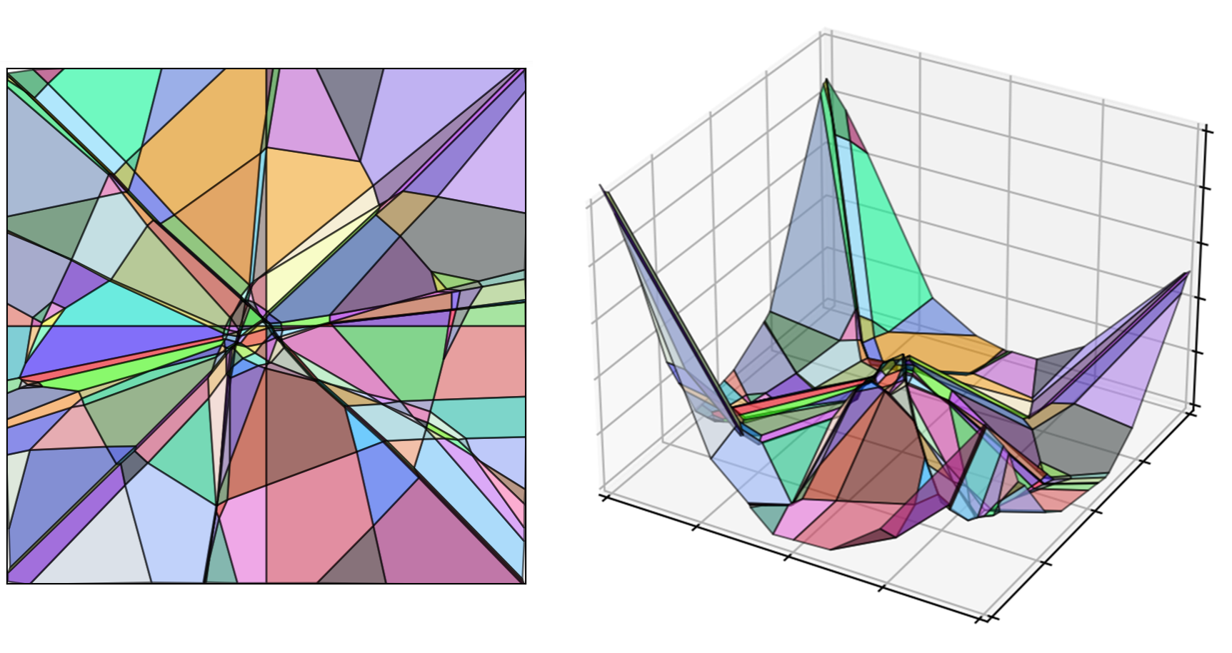
Figure 2: Visual depiction of Eq. 2 with a toy affine spline mapping $S:\mathbb{R}^{2}\rightarrow\mathbb{R}^{3}$. Left: input space partition $\Omega$ made of multiple convex regions shown with different colors and with boundaries shown in black. Right: affine spline image $Im(S)$ which is a continuous piecewise affine surface composed of the input space regions affinely transformed by the per-region affine mappings. Colors maintain correspondence from the left to the right.

More formally and for the context of DNs we will particularly focus on affine splines, i.e., spline operators with $P=1$ and only constrained to enforce continuity throughout the domain.

Let $\bm{S}$ be a Deep Network (DN) with $L$ layers and parameters $\{\bm{W}^{\ell},\bm{b}^{\ell}\}_{\ell=1}^{L}$. Whenever $\bm{S}$ employs continuous piecewise affine (CPA) activation $\sigma$ at each layer, i.e., layer $\ell$ outputs are given by Eq. 1, with $\bm{z}^{0}$ being an input $\bm{x}\in\mathbb{R}^{S}$.

Lemma 1. The layer $1$ to $\ell$ composition of a DN $\bm{S}$, denoted as $\bm{S}^{\ell}$ with output space $\mathbb{R}^{\ell}$, can be expressed as

$$\bm{S}^{\ell}(\bm{x})=\sum_{\omega\in\Omega}\left(\bm{A}_{\omega}^{\ell}\bm{x}+\bm{b}_{\omega}^{\ell}\right)\mathbbm{1}_{\{\bm{x}\in\omega\}},$$ (2)

with indicator function $\mathbbm{1}_{\{.\}}$ and per-region affine parameters given by,

$$\bm{A}_{\omega}^{\ell}= \prod_{i=1}^{\ell}\text{diag}\left(\bm{q}^{i}_{\omega}\right)\bm{W}^{i},$$ (3)

$$\bm{b}_{\omega}^{\ell}= \text{diag}\left(\bm{q}^{\ell}_{\omega}\right)\bm{b}^{\ell}+\sum_{i=1}^{\ell-1}\left(\prod_{j=i+1}^{\ell}\text{diag}\left(\bm{q}^{j}_{\omega}\right)\bm{W}^{j}\right)\text{diag}\left(\bm{q}^{i}_{\omega}\right)\bm{b}^{i}.$$ (4)

Here, $\bm{q}^{\ell}_{\omega}$ is the point-wise derivative of $\sigma$ at pre-activation $\bm{W}^{\ell}\bm{z}^{\ell-1}+\bm{b}^{\ell}$, and $\text{diag}(.)$ operator given a vector argument creates a matrix with the vector values along the diagonal. As a consequence of Thm. 1 from Balestriero et al. [2], $\bm{q}^{\ell}_{\omega}$ is unique for any region $\omega\in\Omega$.

Such formulations of DNs have been extensively employed as it makes theoretical studies amenable to actual DNs without any simplification while leveraging the rich literature on spline theory, e.g., in approximation theory [7], optimal control [8], statistics [9] and related fields.

2.2 Exact Computation of Their Partition and Decision Boundary

Suppose, $\bm{w}_{i}^{\ell}$,$\bm{b}_{i}^{\ell}$ are the $i$-th rows of $\bm{W}^{\ell},\bm{b}^{\ell}$. The following lemma provides us a framework to back-project to ${\mathbb{R}}^{S}$ a hyperplane $h_{i}^{\ell}\in\mathbb{R}^{\ell-1}$ from layer $\ell$ with parameters $\bm{w}_{i}^{\ell},\bm{b}_{i}^{\ell}$, expressed as,

$$h_{i}^{\ell}\triangleq\{\bm{z}\in\mathbb{R}^{\ell-1}:\langle\bm{w}_{i}^{\ell},\bm{z}\rangle+\bm{b}_{i}^{\ell}=0\ \}.$$ (5)

Algorithm 1 Find Partitions

2-polytope $P$ and hyperplanes $\mathcal{H}\in\mathbb{R}^{2}$, s.t., $\mathcal{H}\cap P\neq\emptyset$.

$G,C$. $G=(E,N)$, where $E$ are edges and $N$ are nodes of the graph $G$. $C$ are cycles/cells/faces of $G$.

Step 1: Solve for $N$ = $\{h_{i}\cap(h_{j}\cup P_{e})\leavevmode\nobreak\ \forall h_{i},h_{j}\in\mathcal{H}:j\neq i\}$, where $P_{e}$ are edges of $P$.

Step 2: For each $h_{i}$, sort $\{h_{i}\cap(h_{j}\cup P_{e})\leavevmode\nobreak\ \forall h_{j}\in\mathcal{H}:j\neq i\}$ and connect in sorted sequence to obtain edges $E$.

Step 3: Obtain set of cycles $C$ from graph $G$ via Alg. 2.

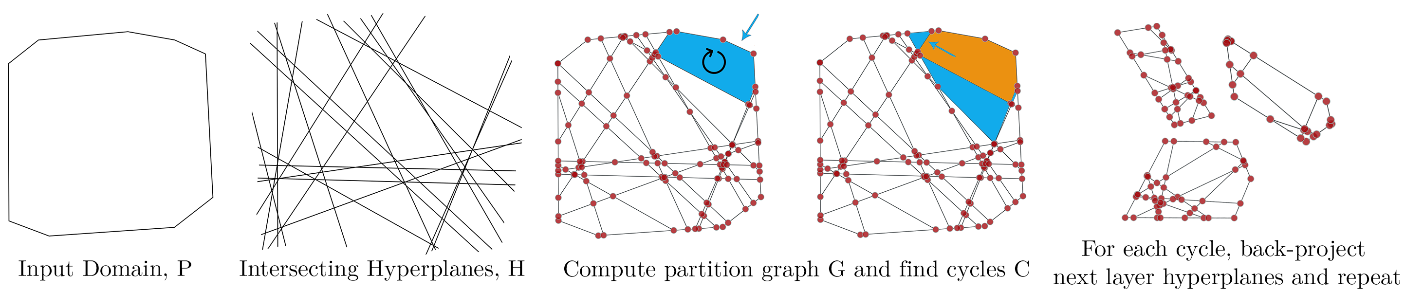
Figure 3: Given an input domain $P$ and a set of hyperplanes $\mathcal{H}$, SplineCam first produces a graph $G$ using all the edge and hyperplane intersections (as in Alg. 1). To find all the cycles in the graph, we select a boundary edge $e_{s}$ (blue arrow), do a breadth-first search (BFS) to find the shortest path through the graph between vertices of $e_{s}$ and obtain the corresponding cycle (blue). The edges obtained via BFS are enqueued and the search is repeated. Each non-boundary edge is allowed to be traversed twice, once from either direction (see Alg. 2). Once new regions are found, we back-project deeper layer hyperplanes, compute partition graphs and repeat.

Lemma 2. Given a hyperplane $h_{i}^{\ell}$, it can be projected onto the tangent space of region $\omega\in\Omega$ as,

$$proj_{\omega}(h_{i}^{\ell})=\{\bm{x}\in\mathbb{R}^{S}:\langle\bm{w}_{i}^{\ell},\bm{A}_{\omega}^{\ell-1}\bm{x}+\bm{b}_{\omega}^{\ell-1}\rangle+\bm{b}_{i}^{\ell}=0\}.$$ (6)

The proof of Lem. 2 is direct since $\bm{z}^{\ell}_{i}=\langle\bm{w}_{i}^{\ell},\bm{A}_{\omega}^{\ell-1}\bm{x}+\bm{b}_{\omega}^{\ell-1}\rangle+\bm{b}_{i}^{\ell}$, with $\bm{z}_{i}^{\ell}$ the i-th element of layer $\ell$ activation.

Theorem 1. Let, $\bm{S}$ is a binary classifier DN therefore with a single output unit. In $\mathbb{R}^{L-1}$, the decision boundary is the hyperplane $h^{L}_{1}$. The decision boundary in $\mathbb{R}^{S}$ is therefore $\cup_{\omega\in\Omega}\{proj_{\omega}(h_{1}^{L})\cap\omega\}$.

Thm. 1 can be proven by repeatedly applying Lem. 2 to back-project the hyperplane $h_{1}^{L}$ for all $\omega\in\Omega$. While the above is general, we want to compute $\Omega$ on a 2-polytope $P\in\mathbb{R}^{S}$ for tractability [1] and ease of visualization.

SplineCam. Let’s denote the partition in the input space formed by the composition of layers $1$ to $\ell$ as $\Omega^{\ell}$. Using Alg. 1, SplineCam starts by partitioning $P$ into $\Omega^{1}$ via hyperplanes $h_{i}^{1}$ from layer $\ell=1$, the first layer. Then for each $\omega\in\Omega^{1}$, we use Lem. 1 and Lem. 2 to obtain $proj_{\omega}(h_{i}^{2})$ for layer two. Therefore, we use Alg. 1 on each region in $\Omega^{1}$ to obtain $\Omega^{2}$. We repeat this for all layers up to $\ell=L$. SplineCam is scalable, all the SplineCam operations can be vectorized except for the search algorithm, which finds cycles in a given graph $G$. We have provided pseudocode for the search algorithm in Alg. 2 and in python script in Suppl. E List. 3.

Algorithm 2 Find cycles

$G=(E,N)$ an undirected graph, $P_{e}\subset E$ boundary edges and starting edge $e_{s}\subset P_{e}$.

$C$ cycles.

Initialize $C=\emptyset,E_{q}=\emptyset$

$G^{\prime}=$bidirectional$(G)$ $\triangleright$ connect edges both ways

APPEND $E_{q}\leftarrow e_{s}$ $\triangleright$ append to end of queue

REMOVE $e_{s}$ from $G^{\prime}$

while $E_{q}\neq\emptyset$ do

     POP $e\leftarrow E_{q}$ $\triangleright$ get from top of queue

     REMOVE $e^{\prime}$ from $G^{\prime}$

$\triangleright$ $e^{\prime}$ is $e$ with its direction inverted

     $E_{c}=$ bfs$(G^{\prime},v_{e},v_{s})$

$\triangleright$ $v_{s},v_{e}$ are start and end vertices of $e$

$\triangleright$ $E_{c}$ are edges forming shortest path from $v_{e}$ to $v_{s}$

     APPEND $E_{q}\leftarrow e_{c}^{\prime},\forall e_{c}\in E_{c}$ if $e_{c}\notin P_{e}$

     REMOVE $e_{c}$ from $G^{\prime}$, $\forall e_{c}\in E_{c}$

     REMOVE $e_{c}^{\prime}$ from $G^{\prime}$, $\forall e_{c}\in E_{c}$ s.t. $e_{c}\subset P_{e}$

     APPEND $E_{c}\leftarrow e^{\prime}$ $\triangleright$ append edge to form cycle

     APPEND $C\leftarrow E_{c}$

end while

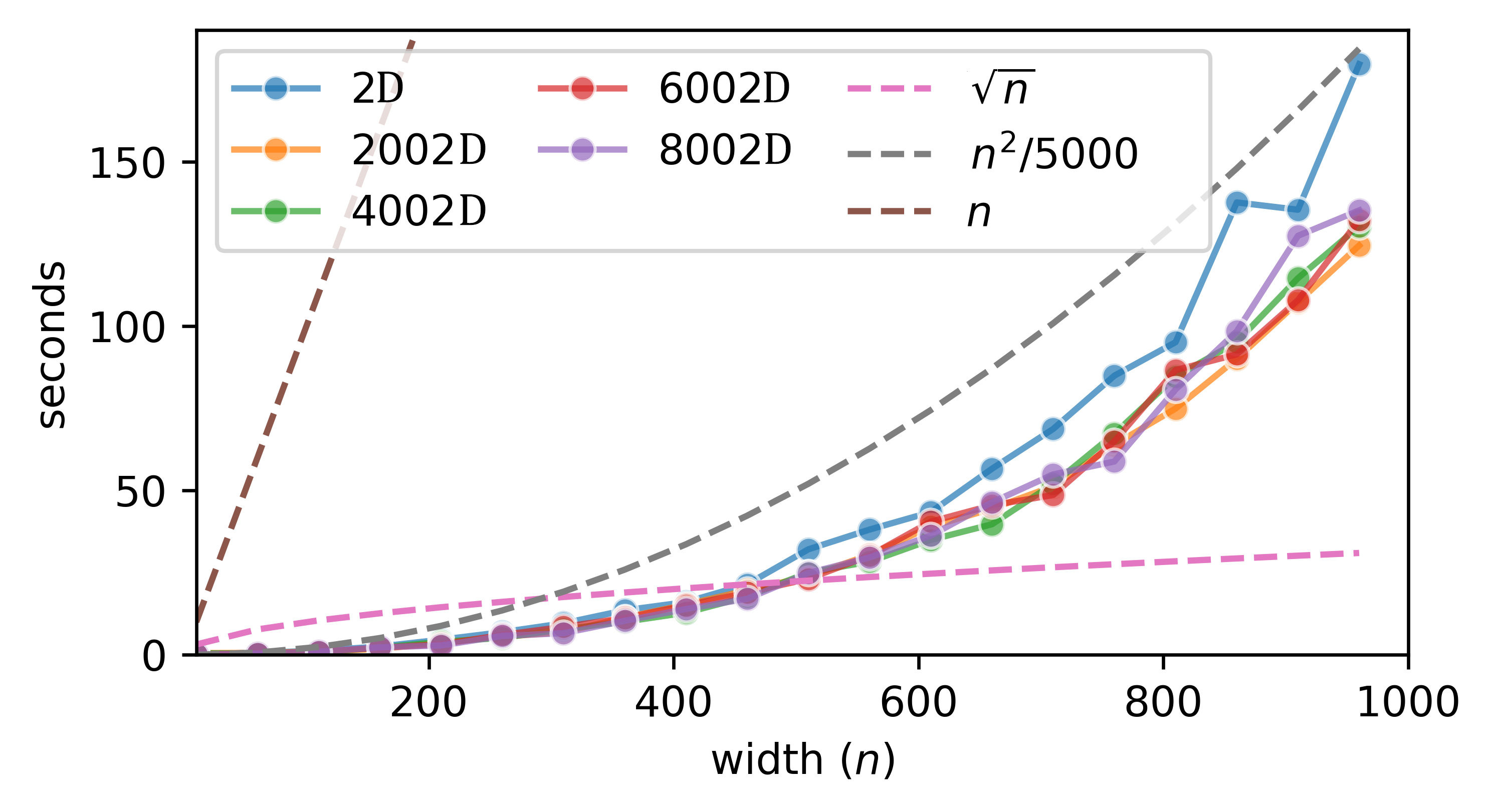
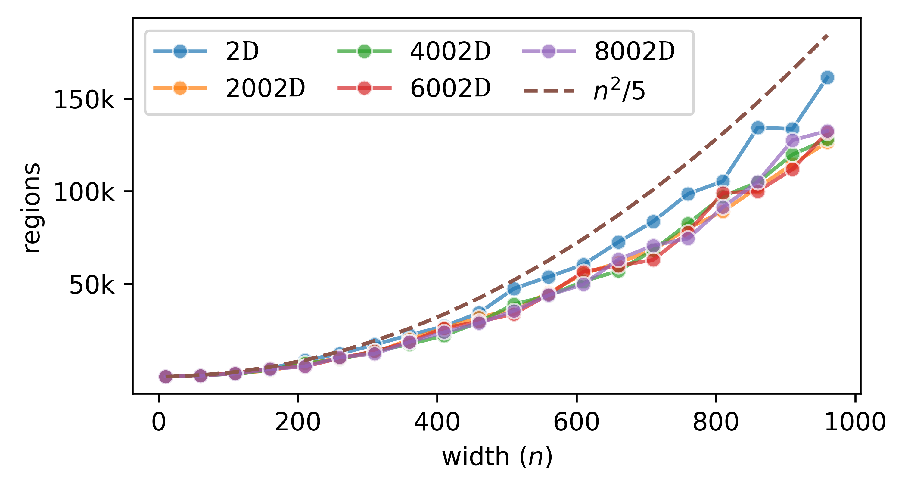
Figure 7: Time complexity of computing the partition regions (Top) and growth of the number of regions with width (Bottom), for a single layer randomly initialized MLP with varying width ($n$) and input dimensionality. For all the input dimensions, we take a randomly oriented, square 2D domain centered on the origin, with an area of $4$ units. Note that with increasing input dimensionality, we get reduced number of hyperplane intersections with our 2D domain of interest, therefore we can see a slight reduction in the wall time required and also the number of regions.

Complexity. For the vectorized operations, we can trade-off time complexity with space complexity by allocating more memory. For Alg. 2, scaling requires distributing sets of $(\omega,\mathcal{H})$ across CPU threads. Given a set of $n$ intersecting hyperplanes and a 2-polytope $P$, the operation of Alg. 1 to find the partition reduces to an arrangement of lines problem. Therefore, the number of intersections, edges and cycles $\leq\mathcal{O}(n^{2})$ [1]. As the number of hyperplanes $n\rightarrow\infty$, the $E[$number of edges per cycle$]$ $\approx\mathcal{O}(1)$, also visible in Table. 1. Therefore, the $E[$complexity$]$ of Alg. 1 as $n\rightarrow\infty$ is also of the order $\mathcal{O}(n^{2})$. In Fig. 7, we present the wall time required for SplineCam for a randomly initialized single layer MLP with variable width and input dimensionality. For an MLP with width $1000$, input dimensionality $8002$, and $8$M params, it takes SplineCam $134s$ to find $132K$ regions. The methods closest to SplineCam in the literature are by Yuan et al. [38] that uses an exponential complexity linear programming based algorithm to compute the DN partitions and Gamba et al. [11] a method that computes the intersection of partition boundaries with one-dimensional lines connecting pairs of training samples. SplineCam is the first exact method that is fast, scalable and computes the partition on 2D slices.

Original image

Layer 1

Layer 2

Layer 3

Layer 4

Layer 5

Reconstruction

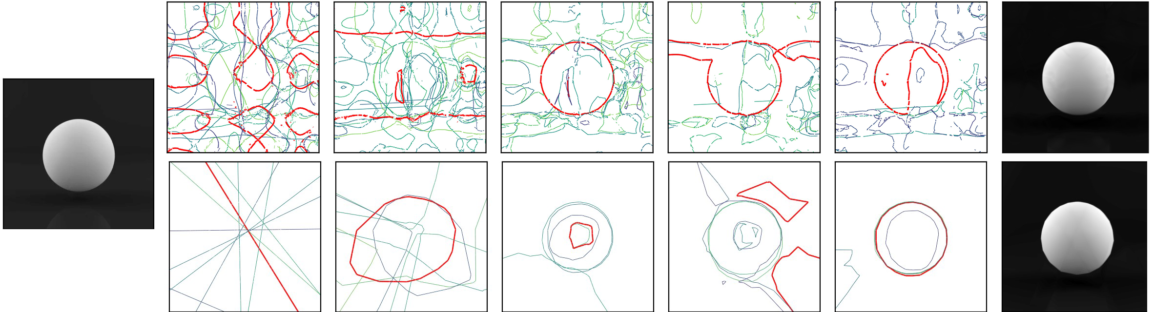
Figure 4: SplineCam visualizations of neurons from different layers of an MLP trained with (top) and without (bottom) periodic position encoding on a 2D image fitting task. All the neurons are visualized in the input space, color coded by the same color, and one neuron from each layer is highlighted in red. The trained MLP has a width of $10$ and depth of $5$ and has ReLU activations for every layer. For the positionally encoded (P.E.) network, boundaries of some neurons seem to be periodically repeating in the input domain, significantly increasing the number of unique $\omega$ where the ReLU is active. The increased weight sharing, i.e., same weights/neurons being used to represent/fit non-contiguous parts of the learned function, could be a possible reason for improved convergence of P.E. MLP [29].

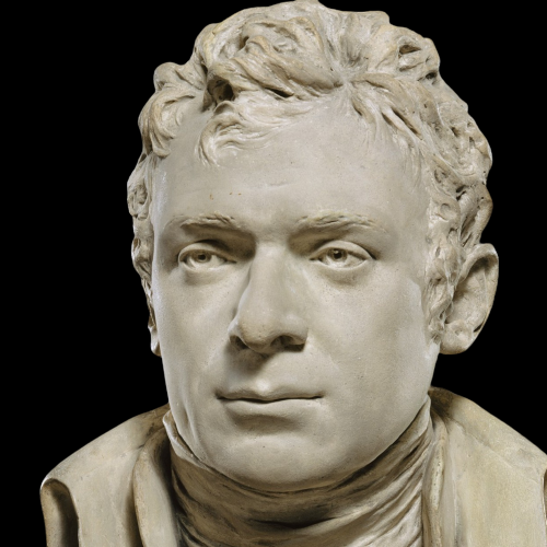
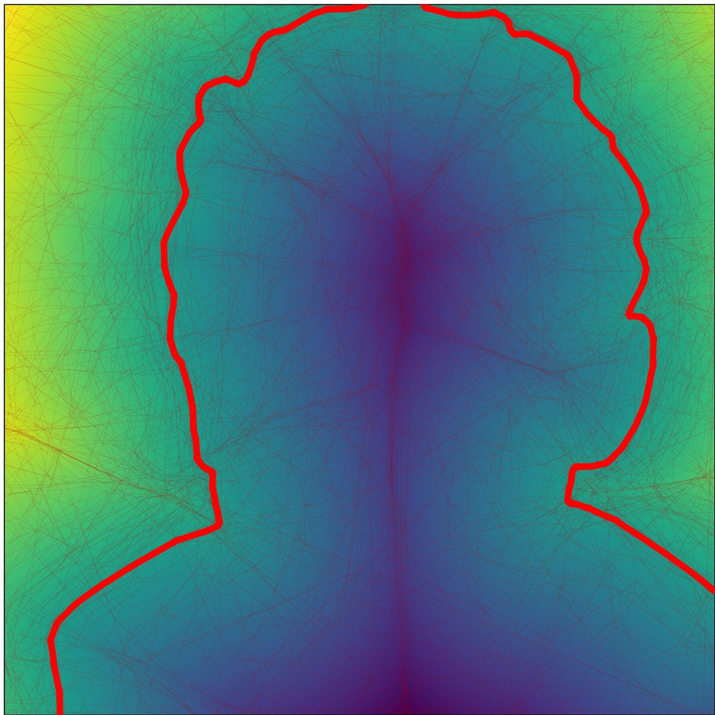
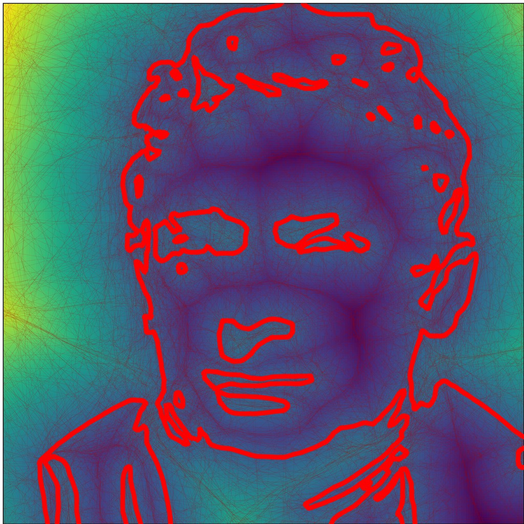
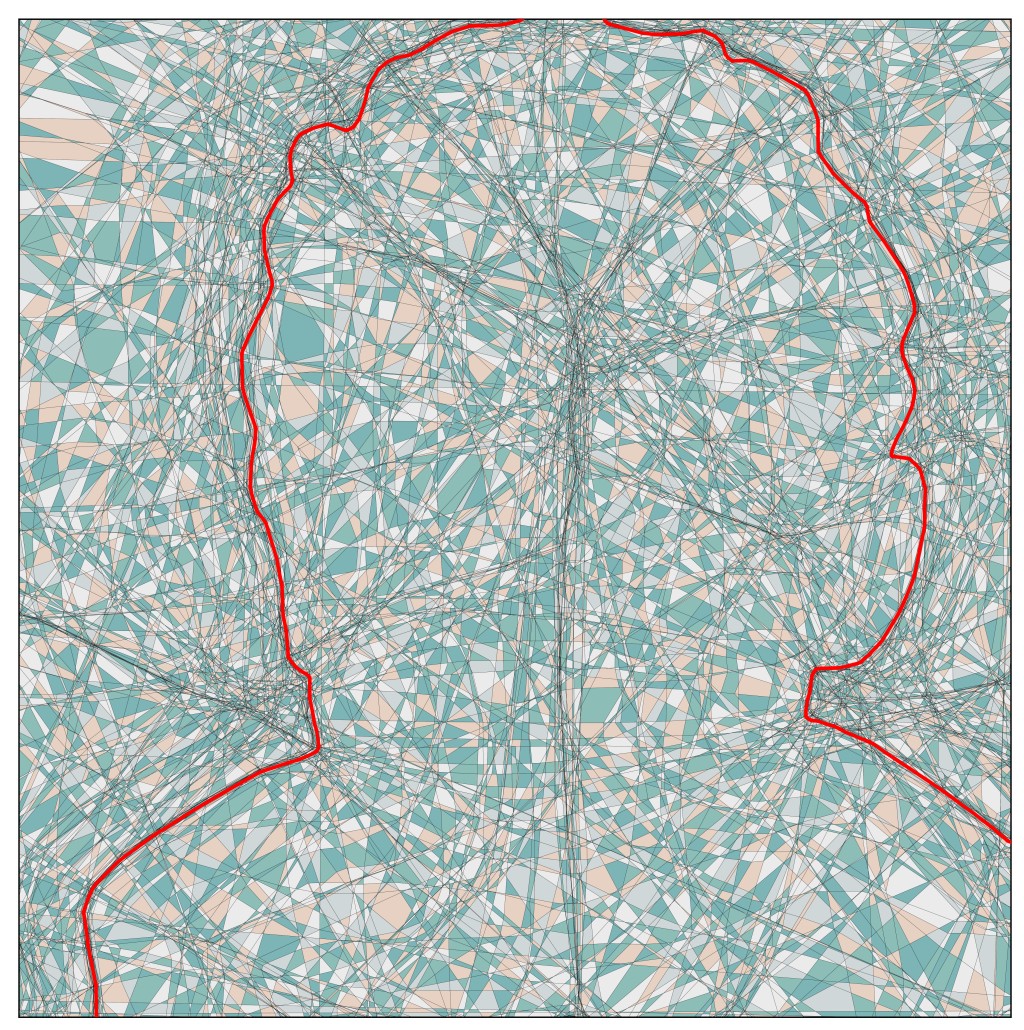
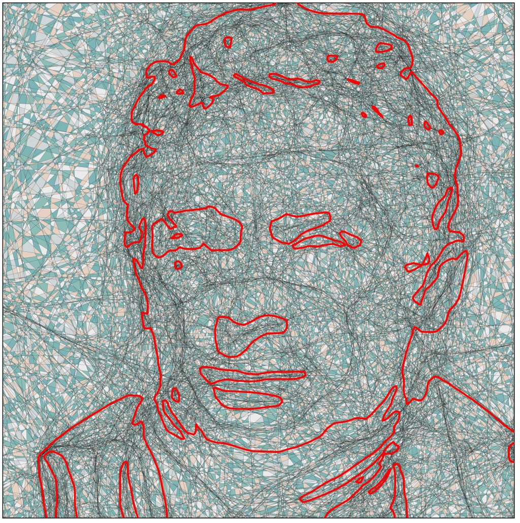
Figure 5: Visualization of the decision boundary and partition geometry of a 2D neural SDF with width $256$ and depth $6$. A single training image is thresholded at $0.01$ and $0.5$ to create two signed distance fields (top middle and right), on which an MLP is trained. For both we can use SplineCam to obtain the analytical zero level set (decision boundary) and also visualize the partition geometry (bottom row). Note that even with identical architecture, the partition density differs significantly based on the task complexity.

3 Visualizing and Understanding Implicit Neural Representations

We start our journey into the geometry of DNs by looking at implicit neural representations (INRs). INRs are pervasive in applications like 3D view synthesis [27] and inverse problems [36], where multi-layer perceptrons are trained to produce a continuous mapping from signal coordinates to the value of the signal at those coordinates. While most state-of-the-art implicit representations require training a single large MLP (parameters in millions) not much has been explored theoretically [41]. For example, while ReLU MLPs were primarily used in NeRF [26]- one of the most popular INR applications- the current practice has moved towards using periodic encodings of the input coordinates and following up with a ReLU-MLP. In this section, we look at the effect of periodic encodings, visualize the geometry of the regions learned by these methods and in the process provide qualitative validation for SplineCam.

3.1 Decision Boundary of Signed Distance Functions

A signed distance function is an implicit continuous representation of a surface or boundary, that outputs the distance of an input from the boundary represented by the function. The zero level set of a signed distance function (SDF) therefore denotes the surface or boundary of the function. Training an INR as a signed distance function is essentially a regression task, where a ground truth distance field is fit by the model to implicitly learn a continuous boundary. We train a 2D and 3D SDF and visualize the analytical zero level set, à la decision boundary, using our method, and visualize the spline partitioning learned by the functions in Fig. 5 and Fig. 1.

To train an INR as a 2D SDF, we take the image as in Fig. 5 from the MetFaces [22] dataset and threshold it at $.001$ and $.05$ to create two binary images. Each binary image is used to create separate ground truth SDFs, one with a simpler boundary separating the background (ESDF) and another with a more convoluted boundary (HSDF). We train an identical ReLU-MLP architecture with width $256$ and depth $6$ on both ESDF and HSDF. In Fig. 5 we present the analytical decision boundary of the SDF overlaid on the ground truth signed distance field for both ESDF and HSDF. While the network capacity remains the same for both, we can see that the spline partition of the two figures vary dramatically, with higher region density for the HSDF task compared to ESDF. For the harder HSDF task, we see the network creating significantly more regions, with higher density, that allows the network to learn the curvature of the decision boundary. This indicates that harder tasks may utilize more of the network parameters compared to easier tasks.

For the 3D SDF task, we train a leakyReLU-MLP with width $256$ depth $6$ on a Stanford Bunny SDF, and present in Fig. 1 the normal map of the learned SDF, as well as the spline partition and decision boundary on three 2D slices, $\{x=0,y=0,z=0\}$. What is noticeable here is that, apart from the final layer hyperplane (final output neuron weights), many neurons from the deeper layers of the network also place their boundaries near the zero level set of the SDF. Meaning, while the decision boundary is denoted by the output neuron, there are multiple neurons that learn parts of the surface boundary. This is a clear indication of the hierarchical nature of signal fitting by INRs.

3.2 The Effect of Positional Encoding on INR Geometry

Table 1: Statistics of the spline partitions formed by fully-connected (MLP) and convolutional neural networks. For each dataset, the same 2D slice and input domain is used to find the partition regions. Convolutional neural networks have a significantly higher number of regions with lower volume compared to MLPs even with less parameters.

Architecture	Dataset	Parameters	Avg Vol	Avg Number of Vertices	Ecc	Number of Regions
MLP	MNIST	44,860	3.144e-4	4	102e7	318
	Fashion-MNIST	44,860	4.991e-4	4	36e7	1364
CONV	MNIST	39,780	1.134e-5	4	17e7	8814
	Fashion-MNIST	39,780	3.54e-5	4	14e7	28222

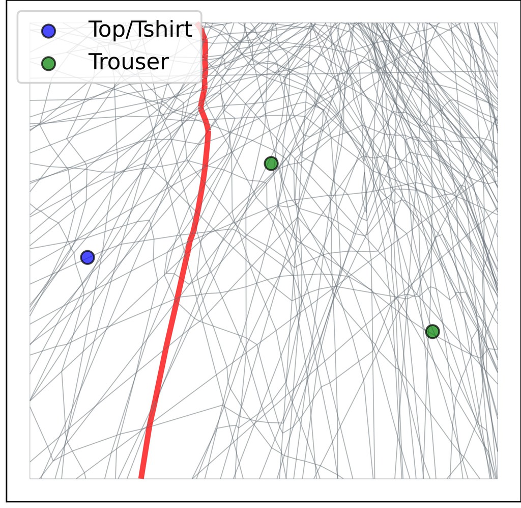
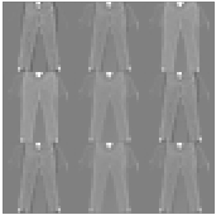
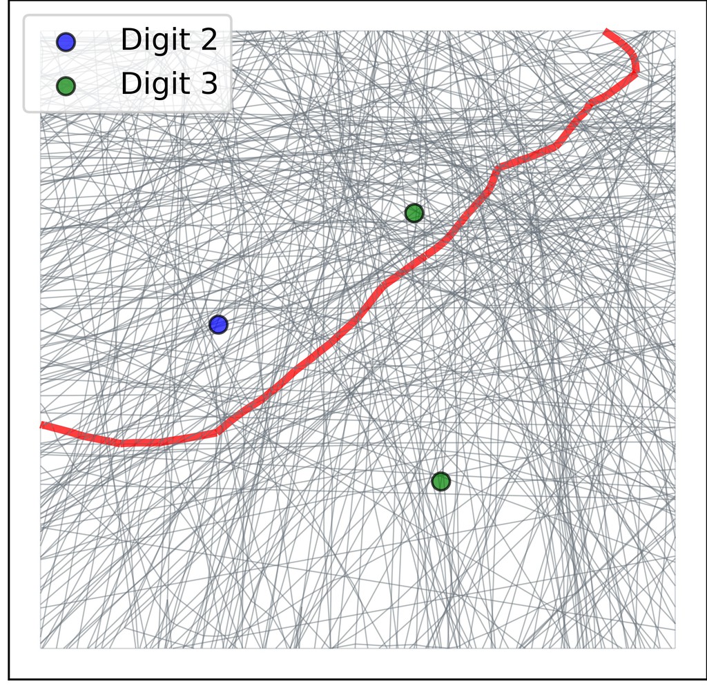
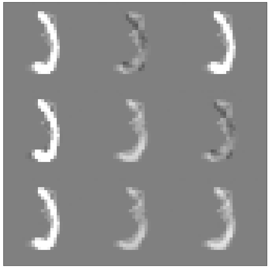
Figure 6: (Top Left) Decision boundary visualization for an MLP with width 50 and depth 3, trained on fashion-MNIST. Dark red line represents the learned decision boundary while black lines represent the spline partition of the network. (Top Right) Samples from the decision boundary between classes Top and Trouser. The samples have distinguishable attributes present from both classes, which indicates a good decision boundary (Bottom Left) SplineCam visualization for a CNN trained on MNIST, with two convolutional layers and one hidden fully connected layer of width 50. One of the digit 3 samples is misclassified by the network as digit 2. (Bottom Right) Samples from the decision boundary between digits 2 and 3 of MNIST. Some of the samples clearly look like the digit three, indicating that the decision boundary here could be sub-optimal.

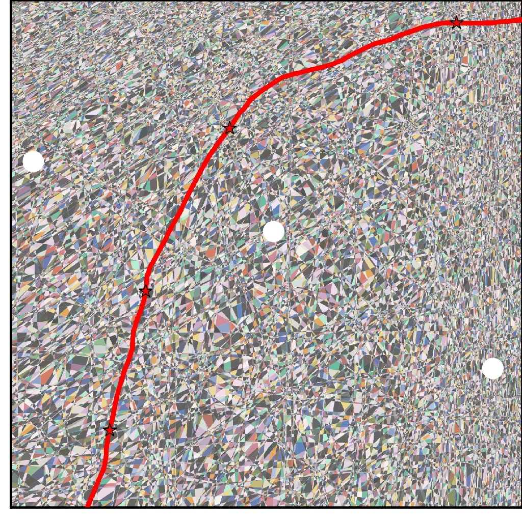
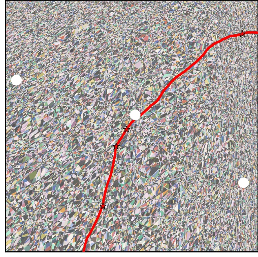
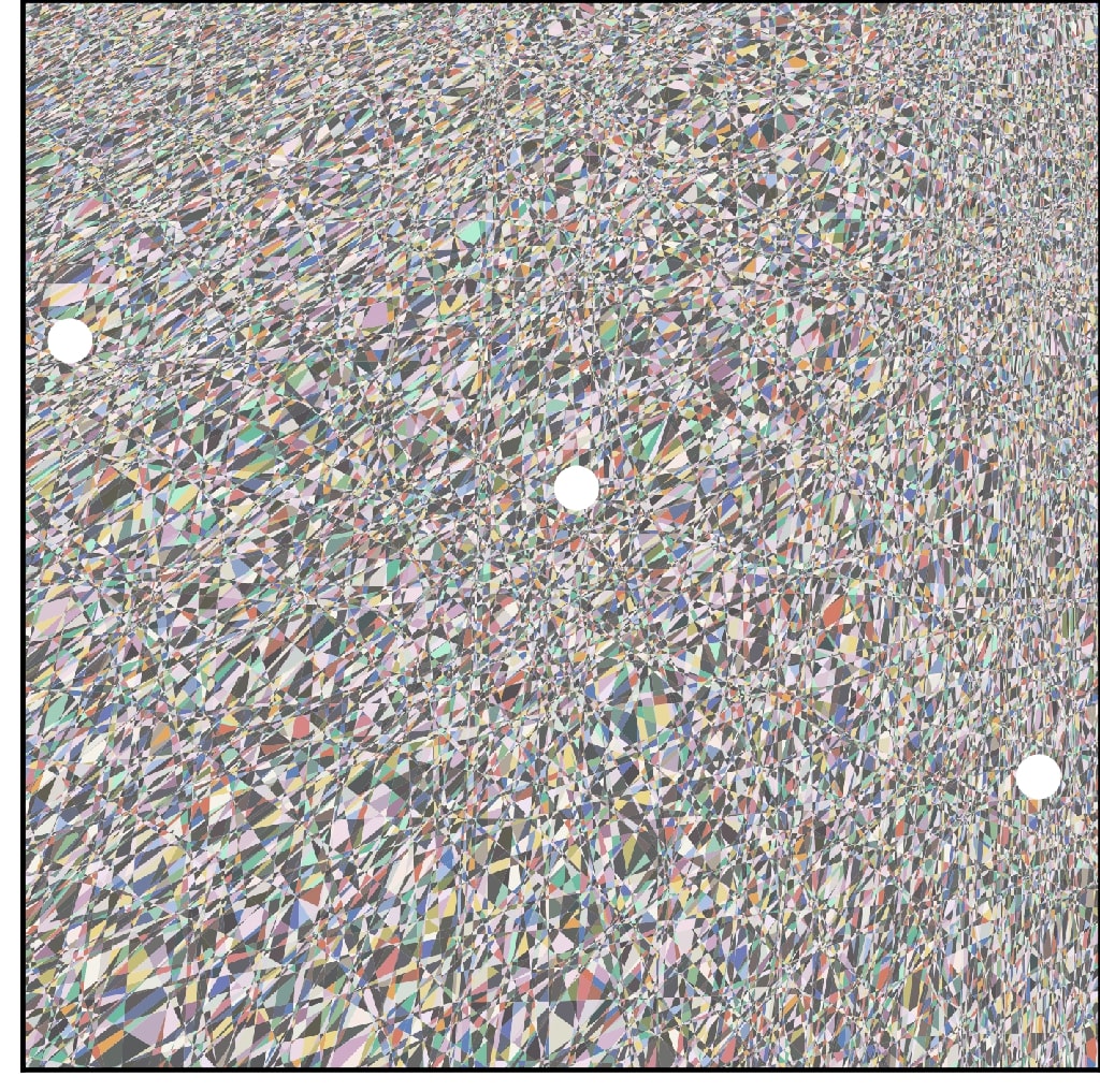
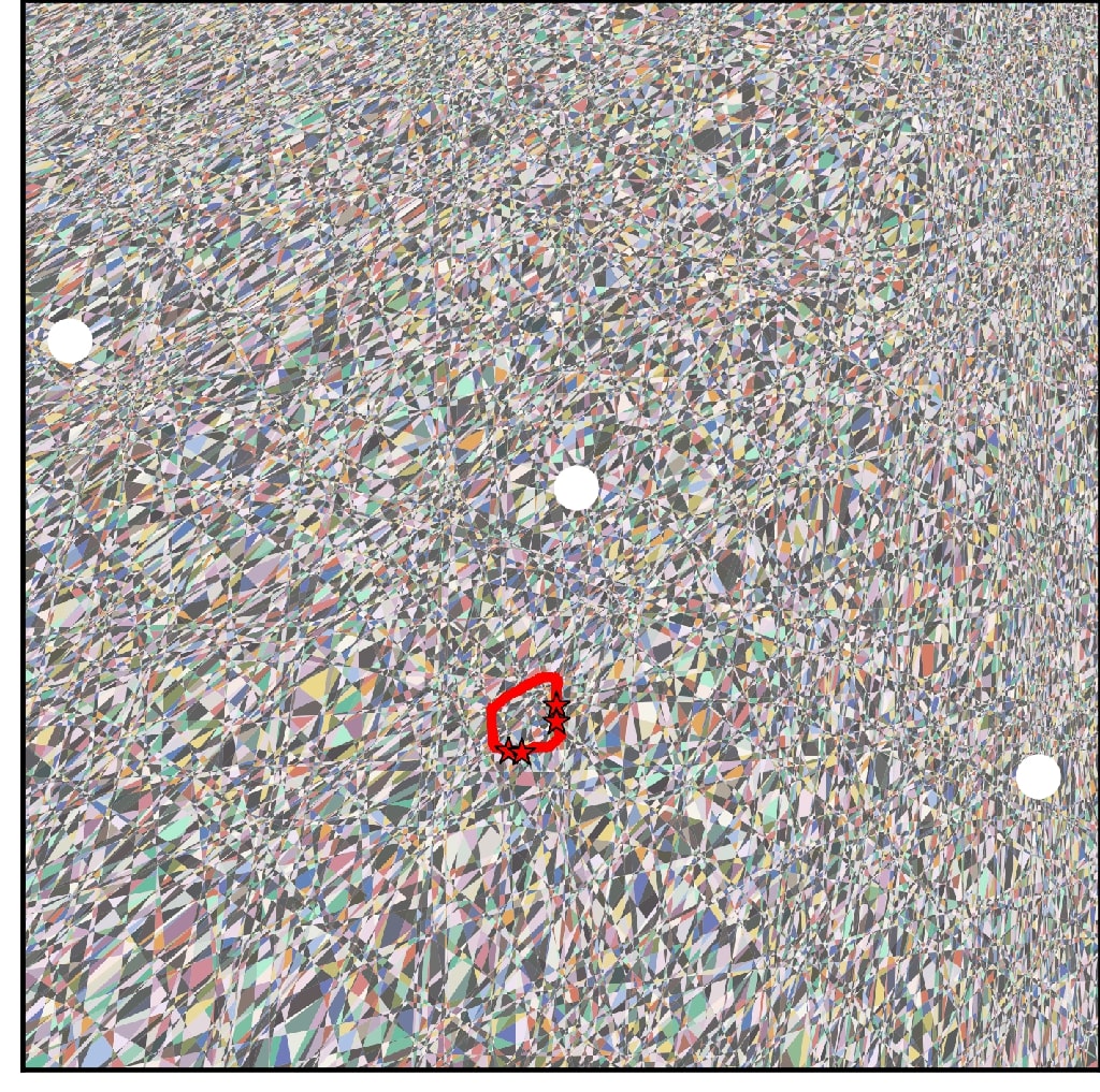
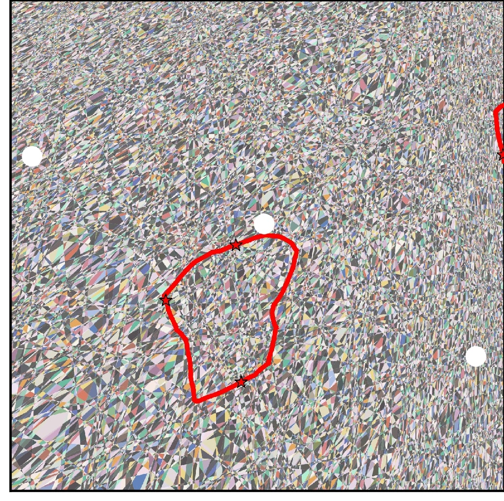
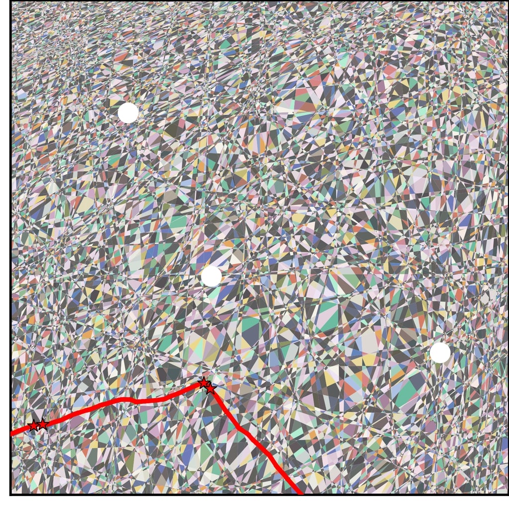
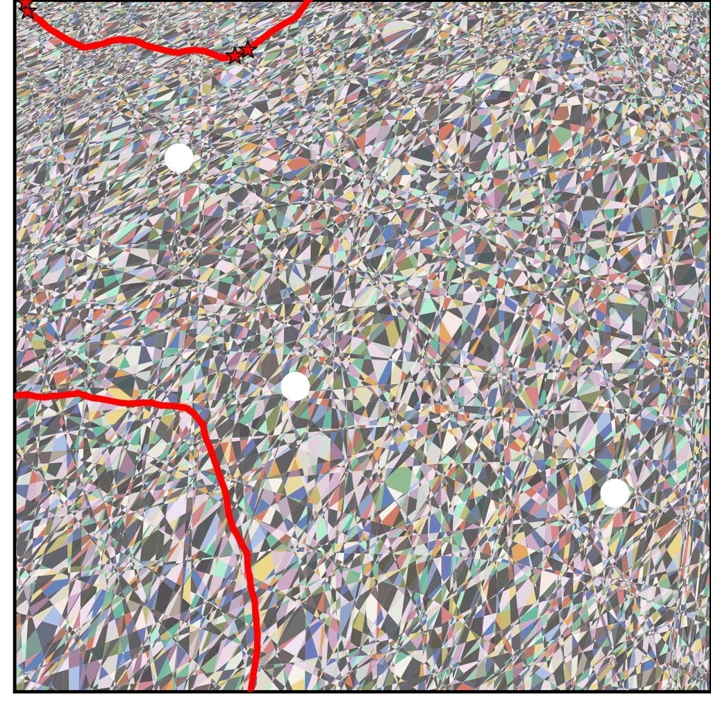
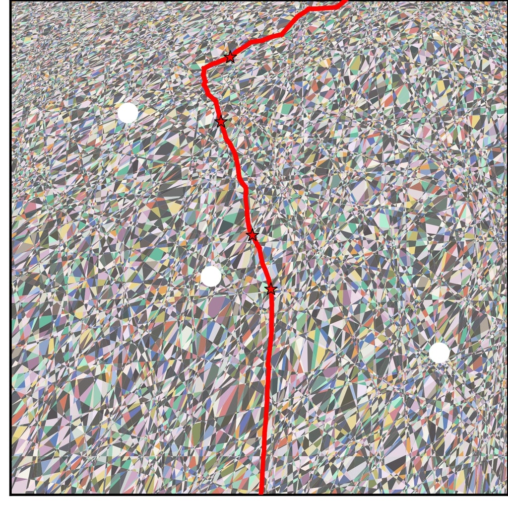
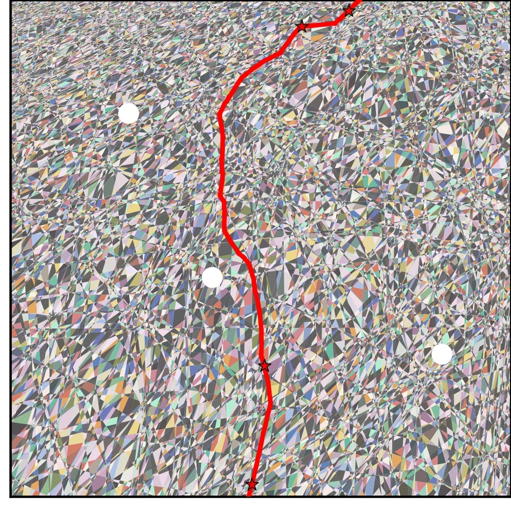
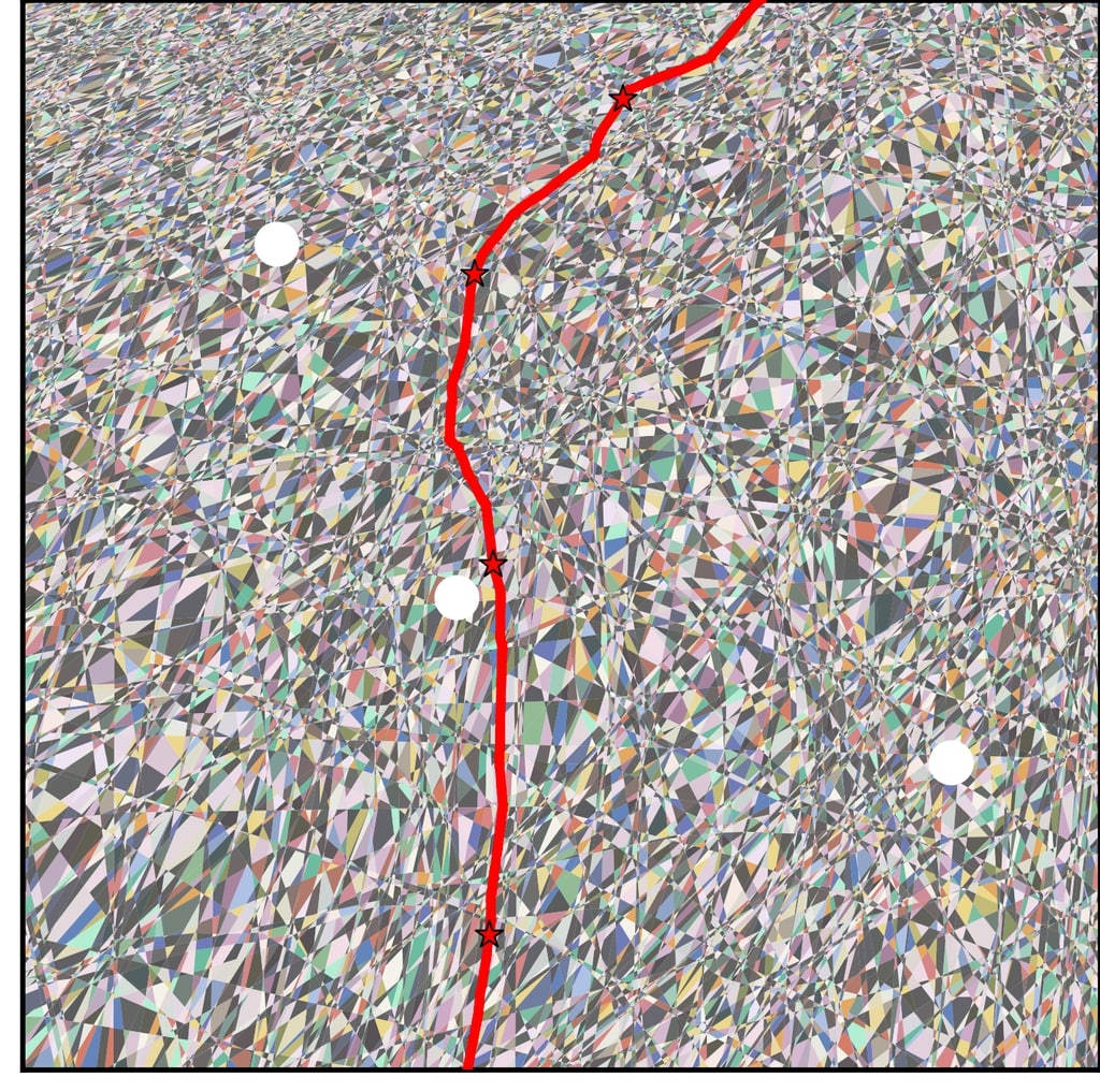
Figure 8: Decision boundary of a $5$ layer convnet during training epochs {50,100,150,200,300} (columns) trained on a binary classification task to classify between Egyptian cat and Tabby Cat classes of tinyimagenet. White points are images from the dataset that were used as anchor points for the $2d$-plane cut in the input space. First, we clearly observe that in the first two columns (epoch 50 and 100) not much change occurs to the decision boundar (red line). However, between epoch 100 and 150, a sudden change occurs making the decision boundary move out of the $2D$-slice, which then slowly recovers until the end of training (top row). On the other hand when looking at a different $2D$-slide of the input space (bottom row) we can see that again between epoch 50 and 100 training does not drastically update the decision boundary, but that between epoch 100 and 150, a sudden change in the decision boundary occurs. It then stays roughly identical (within this slice) until the end of training. Samples from the decision boundary are provided in the appendix.

Empirical evidence shows that INRs trained with periodically encoded coordinates instead of input space coordinates, are able to fit the input signal better with faster convergence rates. While initially inspired by its use in transformer networks there has been very less theoretical investigation of how positional encoding affects learning. We train a 2D INR to regress a grayscale image intensity for given pixel coordinates (Fig.4). We use a ReLU-MLP as the INR backbone, with width $10$ and depth $5$, and visualize the spline partition induced with/without a periodic position encoding front-end. Since SplineCam works with affine non-linearities only, we use a piecewise approximation of sine/cosine while training, with 5 linear regions for each period of the sine/cosine. We see that using this encoding has negligible effect on performance compared to using continuous cosine and sine functions for encoding. In Fig. 4 we present a layerwise visualization where we separately show for each layer the neurons in the input space. We also highlight in red, the boundary induced by a single neuron from each layer.

For the P.E. network boundaries of some neurons seem to be periodically repeating across the input domain. This is due to the periodic wrapping of space induced by P.E., i.e., the input domain is wrapped around in the embedded space which gets cut by subsequent ReLU hyperplanes. The effect of periodicity is most evident for the first layer hyperplanes, as can be seen from the highlighted neuron in Fig. 4. Such repetition of neurons across different parts of the input space, significantly increases the number of regions and weight sharing across input space, which could be a possible reason for improved convergence [29]. We also see a layerwise learning of the boundary of the sphere, indicating how multiple neurons across different depths coordinate to complete the final regression task. The absence of some neurons from the input space domain also shows that not all neurons actively partake in the regression task. For example, while for the first layer of the non-P.E. network, all $10$ hyperplanes intersect the input space, for the last layer only $4$ of the $10$ neurons intersect the input domain. This shows how different neurons create redundancy by remaining active/inactive for all possible inputs.

4 How Training Hyper-Parameters Impact Your Spline

Recall from Sec. 2.1 that any DN with CPWL non-linearities is a CPWL mapping or affine spline. Affine splines have been widely studied and many of their properties, e.g. number of regions in their partition, are known to convey information on the complexity of the function [14]. In this section, we thus propose to take on a more quantitative approach on using SplineCam by quantifying how different training choices, e.g., architecture, data-augmentation, impact the partition of the DN.

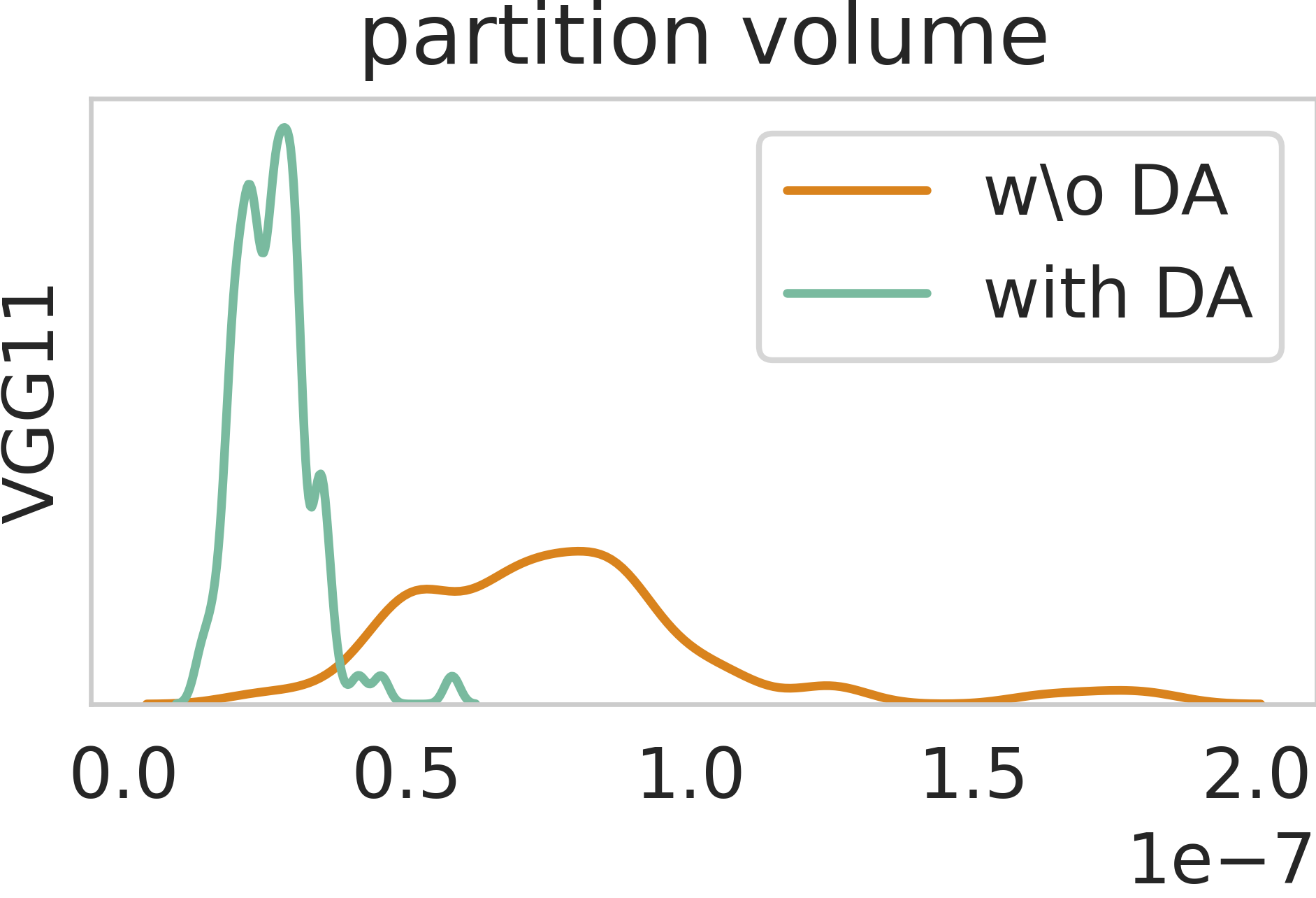
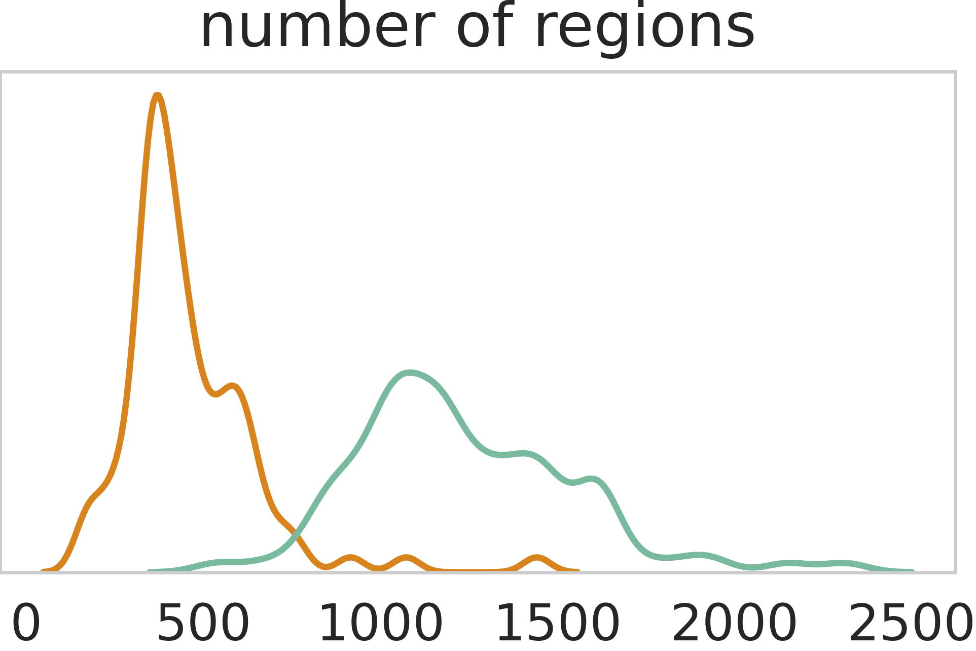
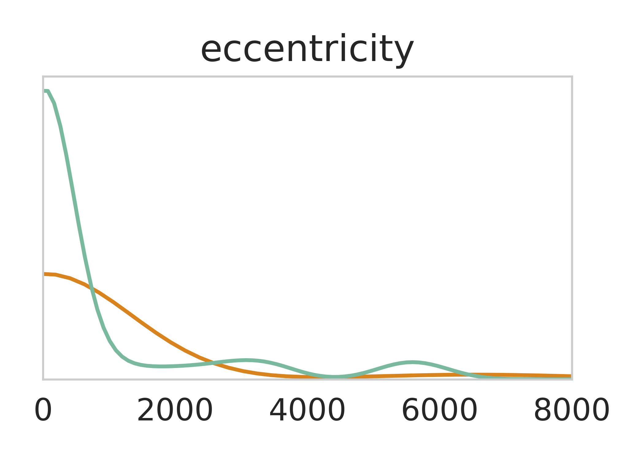
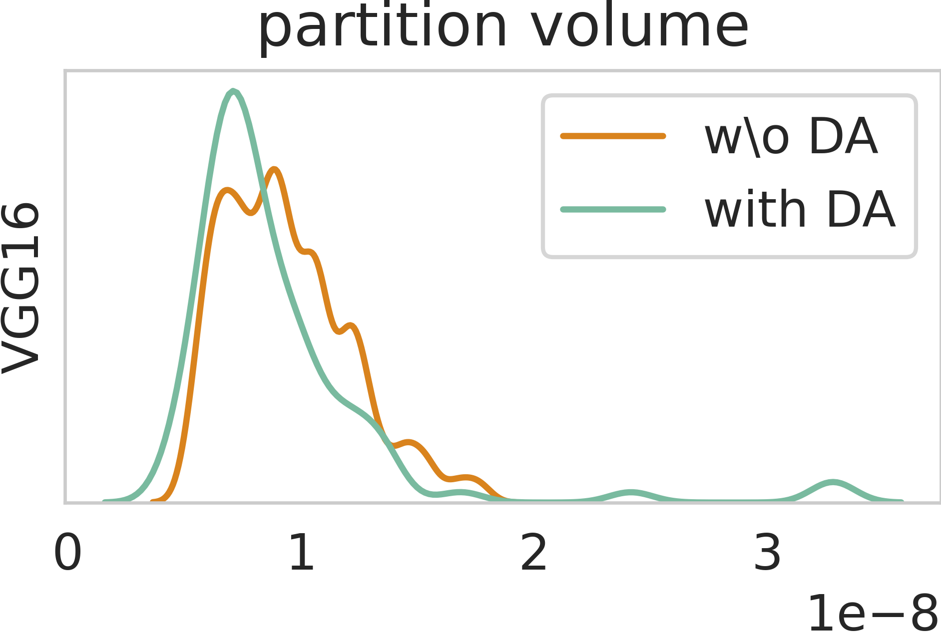
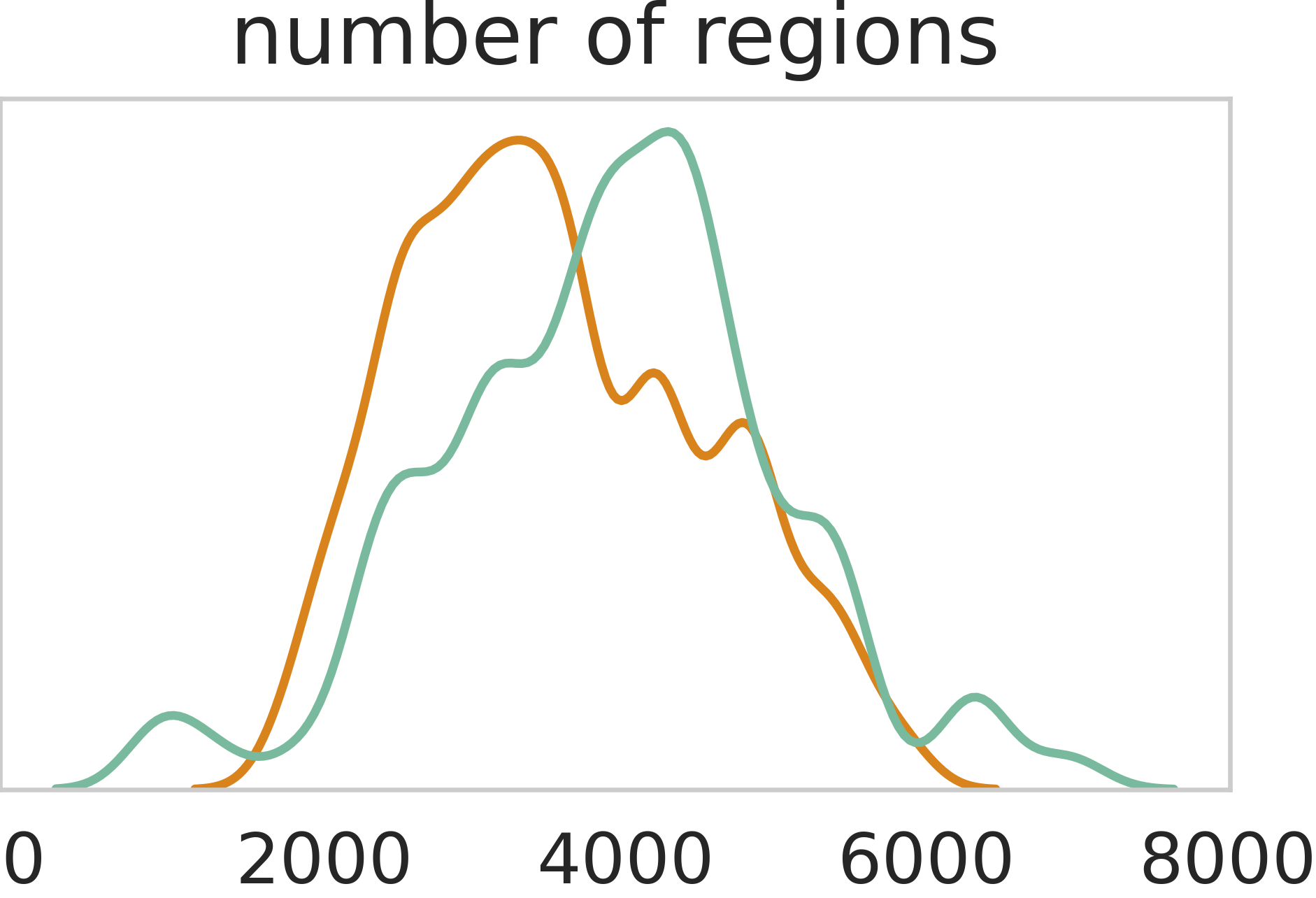
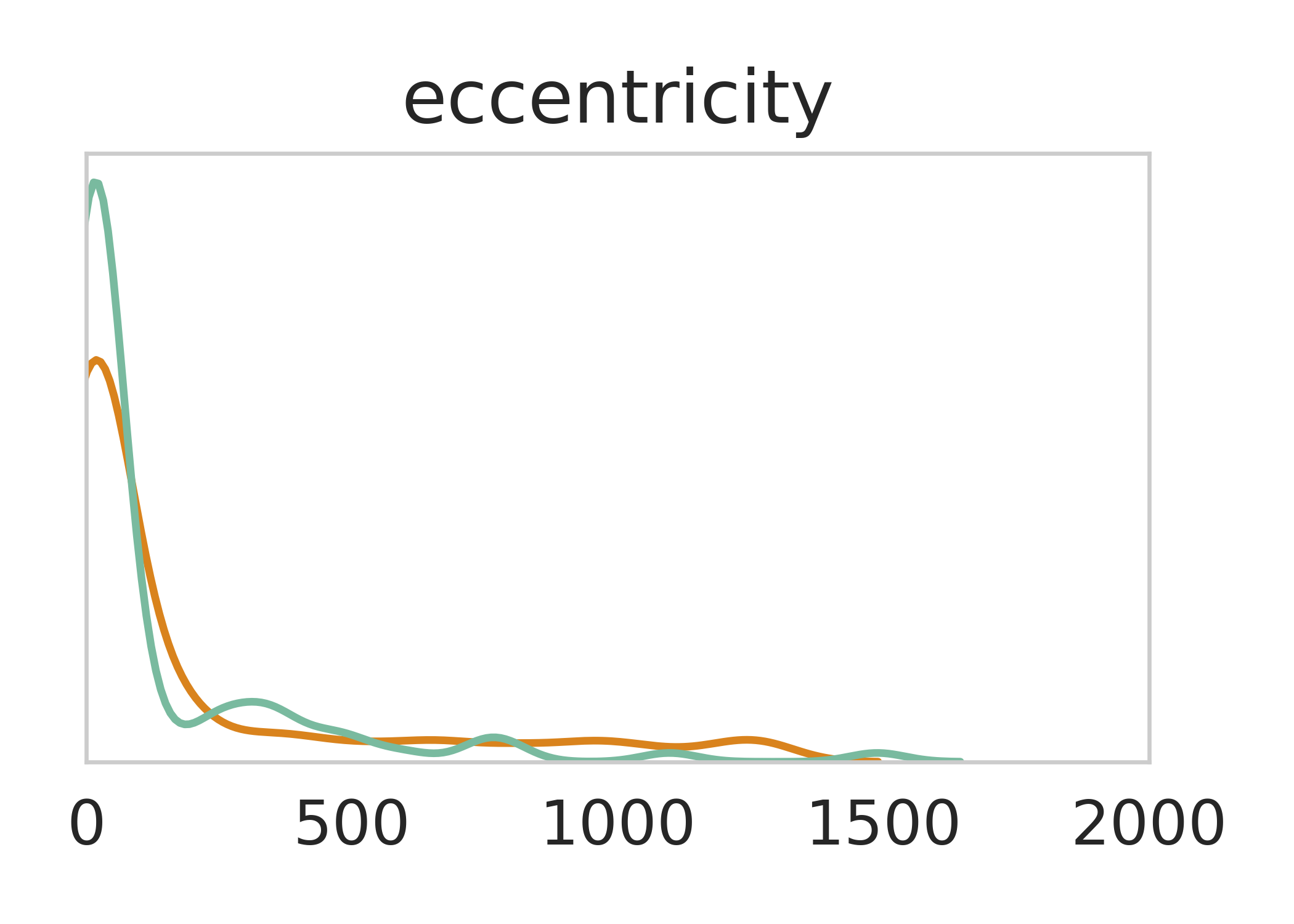
Figure 9: Average partition statistics for 90 tinyimagenet test samples with and without DA training for VGG11 and VGG16. The average volume and number of regions are indicative of partition density whereas eccentricity is indicative of the shape of the regions. For VGG11 a distinct difference in the statistics can be visualized between DA and non-DA training. DA training significantly increases the partition density at test points, which is indicative of better generalizability. On the other hand, the difference reduces for VGG16 while the overall region density increases. This is expected behavior since the VGG16 has significantly more parameters. For both case, the DA models acquired a similar accuracy of $\leavevmode\nobreak\ 51\%$ on the tinyimagenet-200 classification task.

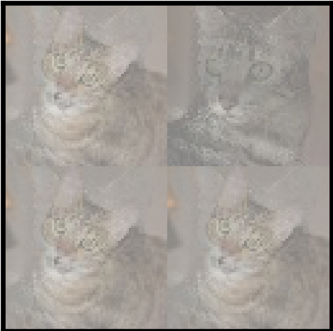
Figure 10: Images from the decision boundary of a CNN trained to perform binary classification between Tabby Cat and Egyptian Cat classes of tinyimagenet. In the supplementary materials we have provided larger sets of images and compare with images obtained from different parts of the input space.

4.1 Impact of Architecture on Partitions Properties

Computing the exact partition boundary finds many applications, not only to visualize and sample the decision boundary (see Fig. 6). We explore some alternative interesting directions in this section.

First, we explore the impact of the DN’s architecture. We see that the choice of architecture can have significant effect on the partitioning induced by a deep neural network (Tab. 1). We quantify the characteristics of the partitions via the following measures- Average Region Volume (ARV), number of vertices, Number of Regions, and eccentricity which is defined as the ratio of the max pairwise distance between vertices and min pairwise distance between vertices. For a given dataset, we fix the input domain and switch between convolutional and fully connected architectures to draw emphasis on the effect of the symmetries induced by a convolutional layer. We see that in convolutional architectures, there is a significantly higher number of partition regions formed, which is an indication of higher complexity of the learned model [28]. We also see that the eccentricity and volume of the polytopes are significantly smaller for convolutional architectures compared to fully connected architectures, indicating more uniform partition shapes and higher partition density. These can also be visualized in Fig. 6. In Suppl. Fig.13 we present the variation of partition statistics with training, for training points, test points and points off the manifold. We see that partition density increases for sample on the data manifold regardless of being on the training.

4.2 Data-Augmentation

Data-Augmentation is a ubiquitous technique that has led to great improvements into DN’s performances [10]. It is still unclear what is the impact of DA onto the DN’s mapping. In fact, while explicit regularizers of DA has been found [17, 5] and while many empirical studies have emerged [39], none truly pinpoint what is different between DNs trained with DA and DNs trained without.

In order to provide a first quantitative understanding of what actually changes within a DN when DA is applied, we propose to rely on SplineCam. In Fig.8 we provide the average volume of region, average number of regions, and mean region eccentricity for spline partitions computer from random 2D domains centered at 90 tiny imagenet test samples. We define region eccentricity to be the ration between the largest and smallest edge for a given region. For each sample, computation of partition statistics take  7mins for VGG11. We see that partition statistics vary significantly between DA and non-DA for VGG11 but not as significantly for VGG16. For both networks, we provide partition visualizations in the supplementary materials. One thing to notice is that the average number of regions more than doubles between VGG11 and VGG16. In the supplementary materials we provide more such comparisons across architecture choices.

5 Conclusions

We present the first provable method to visualize and sample the decision boundary of deep neural networks with CPWL non-linearities. Our presented methods may allow many future avenues of exploration and understanding of neural network geometries. For example, in Fig. 4 in the presented SplineCam visuals, we see that a number of neurons do not intersect the input space domain after learning. We have also seen that number of neurons could be initialized as such that the input vectors always keep the neuron deactivated. Such insights can be used to provide improved initialization or pruning schemes for INRs. Furthermore, using SplineCam we can visualize the decision boundary dynamics of neural networks and asses different training strategies based on decision boundary dynamics across random regions of the input space.

SplineCam: Exact Visualization of Deep Neural Network Geometry and Decision Boundary
Supplementary Materials
Codes available at SplineCAM Github
Google Colab demo https://bit.ly/splinecam-demo

We provide the following supplementary materials (SMs) as support of our theoretical and empirical claims. This SM is organized as follows.

Appendix A provides the necessary background results for SplineCam and elaborates on how any deep neural network or implicit neural representation function with piecewise contiuous affine activations are max affine splines. Appendix B provides further implementation details, extending from Sec. 2.2 and including hardware and software requirements.

Appendix C elaborates on the computational complexity of the method. We present experiments assessing the time complexity of SplineCam varying the width of a single layer MLP and varying the volume of the input domain for VGG11. In Appendix D we present new experiments, first Sec. D.1 discusses the change of partition characteristics with training epochs and while varying architecture parameters (e.g., width for MLP and number of filters for a CNN). We also present the change of characteristics across different parts of the input space, e.g., around training samples, test samples and regions off the data manifold. In Sec. D.2 we present quantitative results on the variation of partition statistics while varying the orientation of the 2D input domain of interest. We see that the variation is considerably low between random orientation, showing that a single 2D slice can possibly be good enough to characterize the partition in different parts of the input space. Finally, in Appendix E we expand on the usage of SplineCam and present code blocks as explainers for how the SplineCam framework operates.

Figure 11: Time complexity of computing the partition regions (Top) and growth of the number of regions with width (Bottom), for a single layer randomly initialized MLP with varying width ($n$) and input dimensionality. For all the input dimensions, we take a randomly oriented, square 2D domain centered on the origin, with an area of $4$ units. Note that with increasing input dimensionality, we get reduced number of hyperplane intersections with our 2D domain of interest, therefore we can see a slight reduction in the wall time required and also the number of regions.

Appendix A Background on Continuous Piecewise Affine Deep Networks

A max-affine spline operator (MASO) concatenates independent max-affine spline (MAS) functions, with each MAS formed from the point-wise maximum of $R$ affine mappings [25, 15]. For our purpose each MASO will express a DN layer and is thus an operator producing a $D^{\ell}$ dimensional vector from a $D^{\ell-1}$ dimensional vector and is formally given by

$${\rm MASO}(\bm{v};\{\bm{A}_{r},\bm{b}_{r}\}_{r=1}^{R})=\max_{r=1,\dots,R}\bm{A}_{r}\bm{v}+\bm{b}_{r},$$ (7)

where $\bm{A}_{r}\in\mathbb{R}^{D^{\ell}\times D^{\ell-1}}$ are the slopes and $\bm{b}_{r}\in\mathbb{R}^{D^{\ell}}$ are the offset/bias parameters and the maximum is taken coordinate-wise. For example, a layer comprising a fully connected operator with weights $\bm{W}^{\ell}$ and biases $\bm{b}^{\ell}$ followed by a ReLU activation operator corresponds to a (single) MASO with $R=2,\bm{A}_{1}=\bm{W}^{\ell},\bm{A}_{2}=\mathbf{0},\bm{b}_{1}=\bm{b}^{\ell},\bm{b}_{2}=\mathbf{0}$. Note that a MASO is a continuous piecewise-affine (CPA) operator [37].

The key background result for this paper is that the layers of DNs constructed from piecewise affine operators (e.g., convolution, ReLU, and max-pooling) are MASOs [2]:

$$\exists R\in\mathbb{N}^{*},\exists\{\bm{A}_{r},\bm{b}_{r}\}_{r=1}^{R}$$ (8)

$$\text{ s.t. }{\rm MASO}(\bm{v};\{\bm{A}_{r},\bm{b}_{r}\}_{r=1}^{R})=g^{\ell}(\bm{v}),\forall\bm{v}\in\mathbb{R}^{D^{\ell-1}},$$ (9)

making any Implicit Neural Representation or even Deep Generative Networks a composition of MASOs.
The CPA spline interpretation enabled from a MASO formulation of DNs provides a powerful global geometric interpretation of the network mapping based on a partition of its input space ${\mathbb{R}}^{S}$ into polyhedral regions and a per-region affine transformation producing the network output. The partition regions are built up over the layers via a subdivision process and are closely related to Voronoi and power diagrams [4].

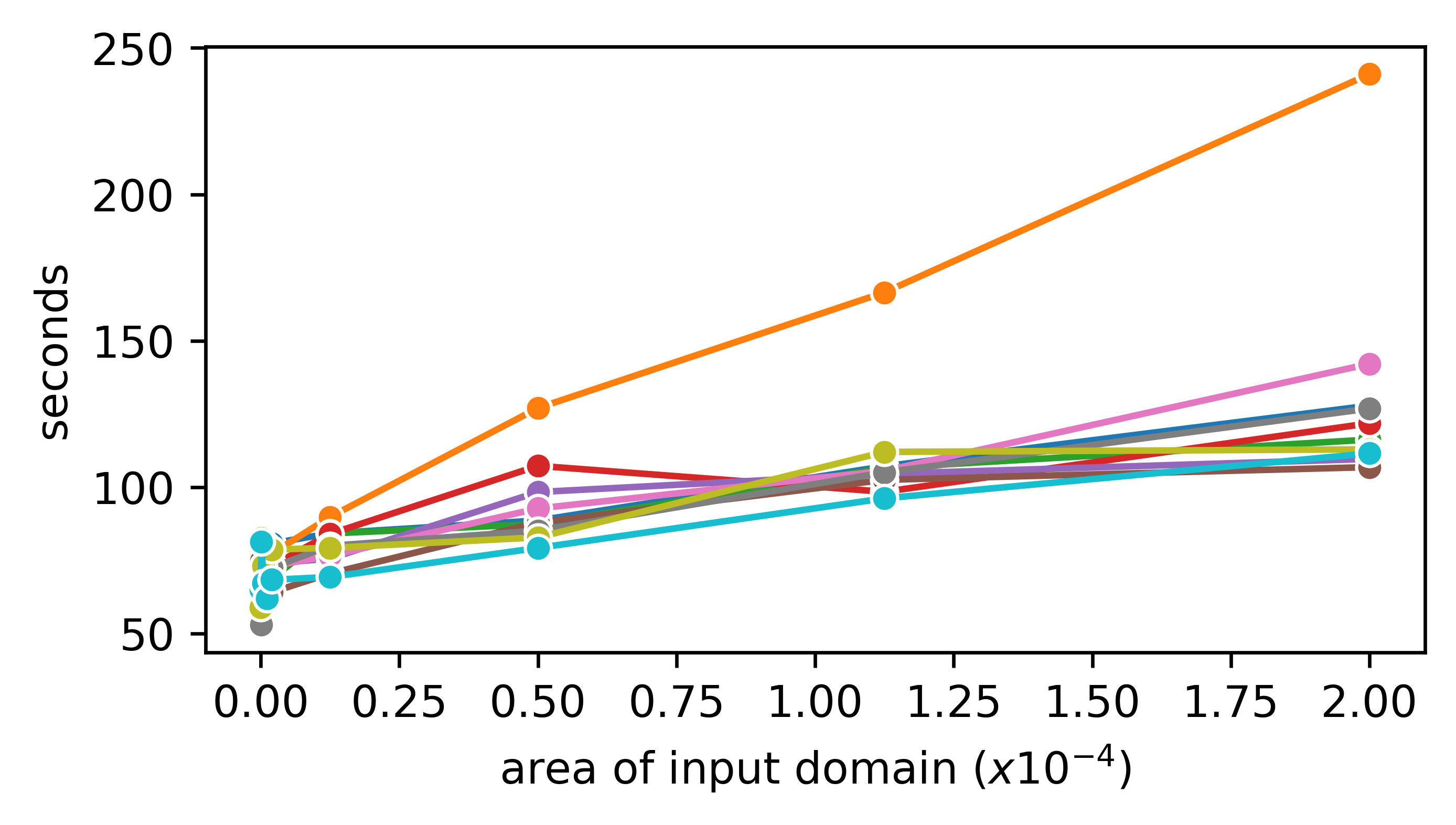
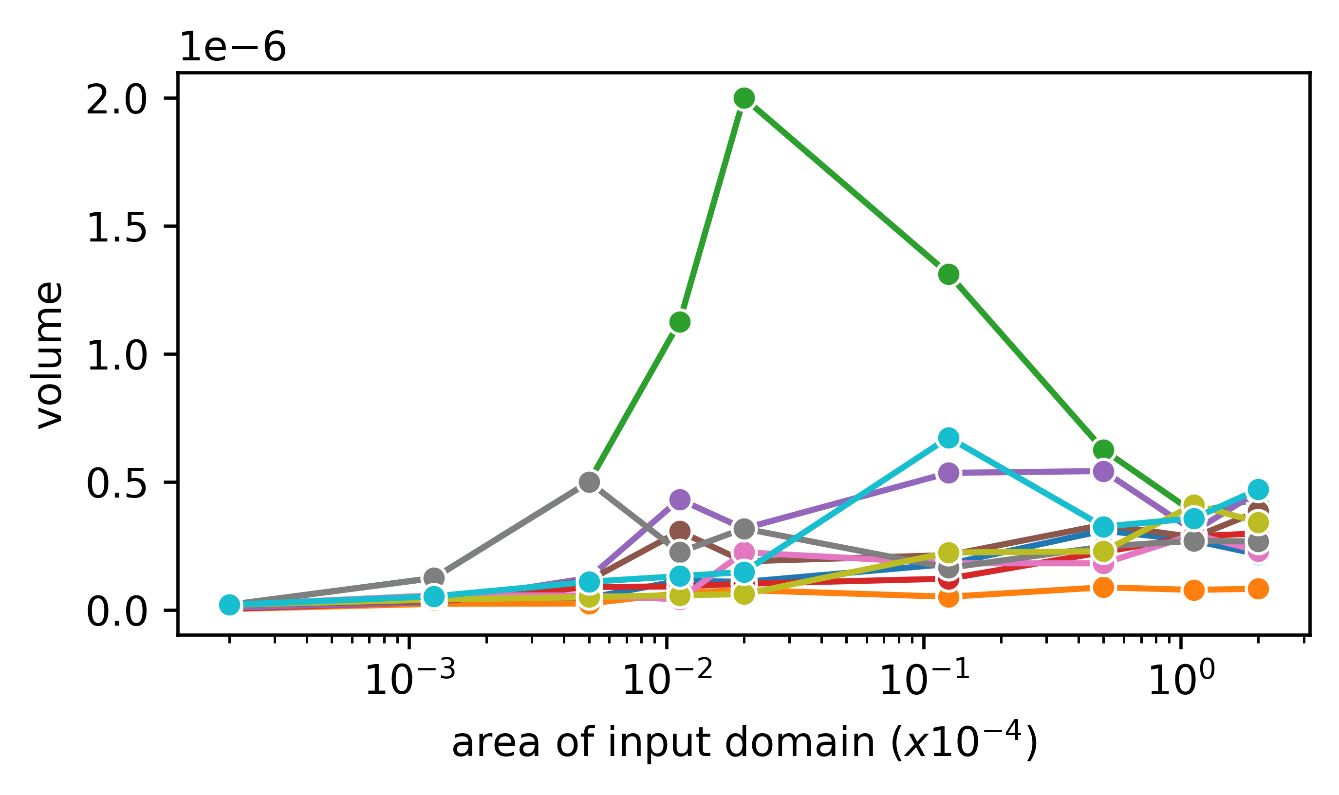
Figure 12: Time complexity of computing the partition regions Top and average region volume (ARV) Bottom while increasing the area of the input domain, for a VGG11 trained on tinyimagenet-200. Each line corresponds to one of $10$ training samples anchored on which the 2D input domains are defined, with random orientations. We see that the required time scales linearly with the size of the input domain. Apart from that, we see that as the neighborhood size is increased for some samples, the ARV increases and then decreases again. This could indicate that while the ARV is small for smaller neighborhoods around training samples while farther away larger regions appear and cause the transient behavior in the curves.

Appendix B Implementation Details

In Sec. 2.2 we provide a summary of how SplineCam works. In this section we provide details about SplineCam implementation and algorithm.

SplineCam is implemented using Pytorch [30] and Graph-tool [31]. All the linear algebra operations are performed using Pytorch and are scalable using GPUs. The region finding operation on the other hand is single threaded. This can be a bottleneck in cases, for example, with DNNs that have more than one layer. In this case, distributing regions across threads, as pairs of hyperplane-sets and a polygon, can result in significant speedups.

Since finding the regions involve solving systems of linear equations, most of the opearations in SplineCam require double precision. This can introduce significant memory bottlenecks, especially for large convolutional layers with multiple channels of input and output; for such layers the size of the corresponding Toeplitz matrix representation becomes significantly large with large number of input and output channels. For this reason, we always store such weight matrices as sparse matrices and query rows only when required. We also replace max pool layers with average pool layers for simplicity; in our experiments involving VGG16 and VGG11, we replace the maxpool after the first conv with an average pool and use strided convolutions for deeper layers. Unless specified, we always consider square 2D domains in the input. While characterizing we use the terms volume and area of the regions interchangeably.

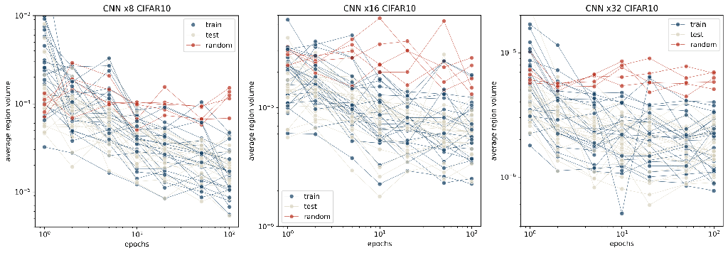
Figure 13: Evolution of average region volume (ARV) for $55$ different randomly oriented square domains of the input space. Out of the $55$ domains, $25$ are centered on CIFAR10 training samples, $25$ on test samples and $5$ on random locations in the input space. We train a $8$ layer CNN as detailed in Appendix. D.1. We notice that as training progresses, the ARV around points on the data manifold gets reduced. For points off the manifold ARV reduces as well, for CNN x8 CIFAR10 it reduces significantly while for CNN x32 it doesn’t. In all cases, the off manifold ARV remains larger than the on manifold ARV at 100 training epochs.

In Appendix. E, we provide details on how SplineCam can be used, with modular codes showing how it computes the partition in a layerwise fashion. We also provide a pseudocode for the search algorithm we have proposed to find regions given a graph formed via polygon-hyperplane intersections. All the reported computation times were evaluated on a setup consisting of 8x NVIDIA QUADRO RTX 8000 48GB GPUs and 2x Intel Xeon Gold 5220R.

Appendix C Computational Complexity

In this section we present two sets of experiments that we have performed to assess the computational complexity of SplineCam.

Varying width for a single layer MLP. As we have discussed earlier and have elaborated in Appendix. E, SplineCam performs region wise partition operations, which can be parallelized across sets of regions. To assess the per region performance of SplineCam, we do the following experiment. We take an uninitialized 1 layer ReLU-MLP with $n$ neurons and $D$ input dimensionality. The number of neurons is equal to the number of hyperplanes that would partition space. We vary $n\in\{10...980\}$ and also vary $D\in\{2,2002,4002,6002,8002\}$ and plot in Fig. 11 the wall time in seconds, required to compute the partition. As the input domain, we consider a randomly oriented 2D domain centered on the origin with $4sq$ unit area. We see that the computation time complexity is upper bounded by $\mathcal{O}(n^{2}/5000)$ within the range of $n$ in question. With increasing $D$ we see a reduced number of hyperplane intersections, therefore we see a reduction in required time.

Effect of the area of the input domain. For this experiment, we take a VGG11 model and increase the size (area) of the input domain. We present the wall time vs area plot in Fig. 12. We can see that increasing the area (or volume) of the input region, monotonically increases the required time for computing the partition, in approximately a linear fashion. Even though increasing the area of the input domain should increase the number of first layer intersections, we see that the effect of that remains linear within the range. Note that, we can also scale the area of the input domain by breaking the input domain into multiple 2D polygonal regions of equal area and using separate threads/gpus to perform computation. This way we can also parallelize the partition computation and scale across memory instead of time.

Appendix D Extra Experiments

D.1 Evolution of partition statistics while training

MLP trained on MNIST. For this experiment we train an MLP with depth $5$ and width $\in\{8,16,32,16,128\}$. We train the MLPs for $50$ training epochs on the MNIST dataset, and evaluate the partition statistics via SplineCam, for $25$ training and $25$ validation samples of randomly selected from MNIST. We present average region volume (ARV) distributions per training epoch in Fig. 15. The first thing to notice is that for smaller width networks, ARV is bimodal across all epochs, while for width 64 and onwards, the mode with higher volume regions vanishes. ARV also shifts towards lower volumes as the width of the networks are increased. While training samples tend to have lower ARV, the lower ends of the distributions differ between training and test samples; for widths 32, 64, and 128 we see distinct low ARV tails which are not visible for the test samples. This shows that for some of the training samples, the partition regions of the network are smaller, indicating that the model has more representation capacity for such sample neighborhoods [28]. This could be a possible indication for memorization of some training samples. Another thing to notice is that during the first epoch, the avg partition volumes are significantly lower. As training progresses, first ARV shifts to the right (larger) and then slowly shifts to the left. As we increase width, the starting ARV of the network becomes small in general compared to the ARV for the last training epoch. In Fig. 16 we also present the distributions of the average number of regions (ANR) in the neighborhood of the same samples used for Fig. 15.

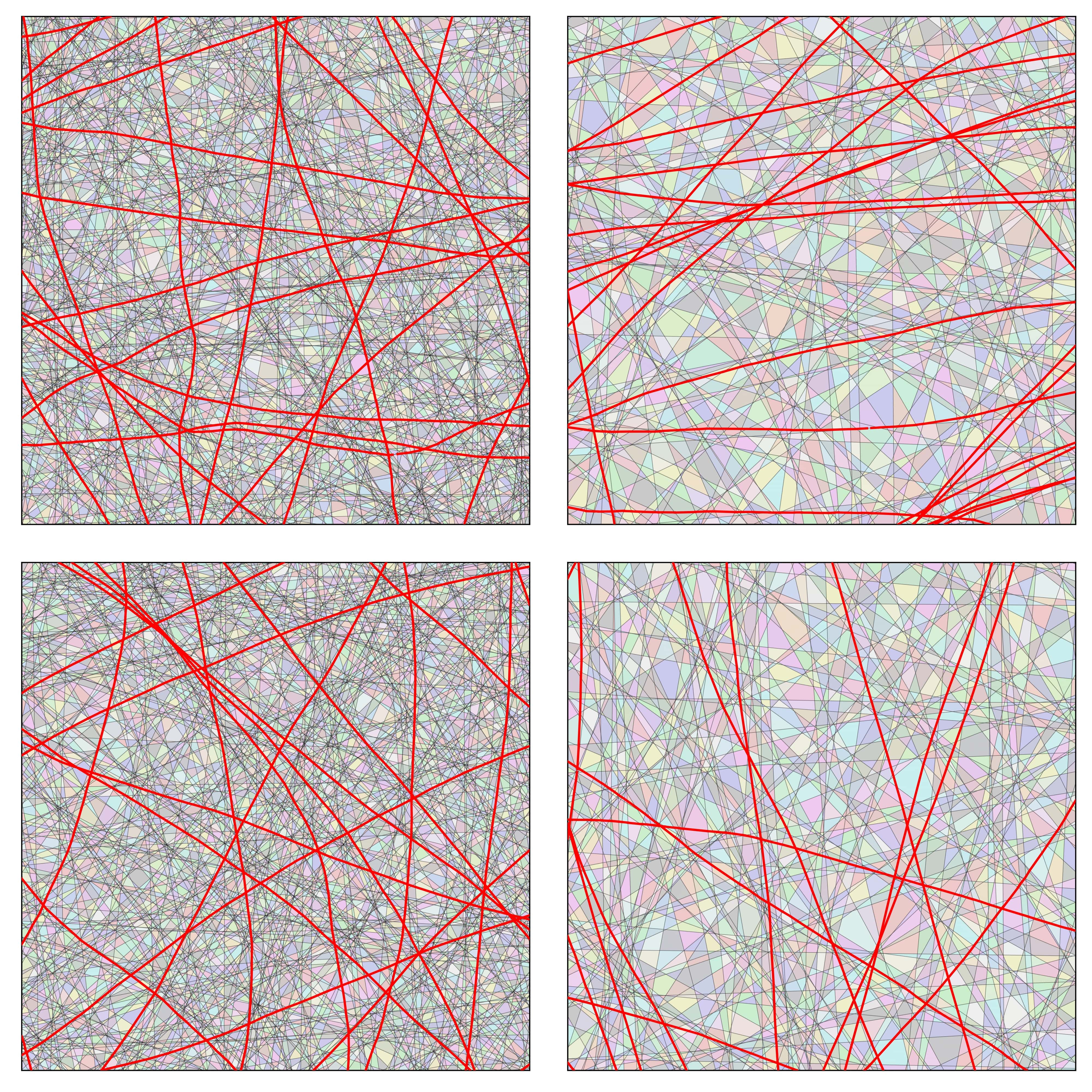
Figure 14: Partition visualization for a VGG11 model trained on TinyImagenet. We take 10 samples from the training set for which the model posteriors have the lowest entropy, and present here neighborhoods for two samples with high partition density (Left) and two samples with low partition density (Right). We also highlight in red, the sets of points for which any two classes from the dataset has equal probability. We see that the denser partition regions have more such lines compared to sparser regions, suggesting correlations with generalization [34]

CNN trained on CIFAR10. For this experiment, we train an $8$ layer CNN with $6$ convolutional layers and $2$ fully connected layers. The number of filters for the convolutional layers are set as $\{\lfloor\ell/2\rfloor\times mul\ :\ell=1...6\}$, where $\lfloor.\rfloor$ is the floor operation, and $mul\in\{8,16,32\}$ is a width multiplier. We see that, similar to Fig. 15, the ARV gets reduced with increased width. For training, we can see longer tails towards lower ARV, indicating denser regions near some training samples. One thing that is noticeable here is that contrary to MLPs, the ARV of neighborhoods near training samples monotonically decrease in most cases for the CNNs. This could be due to the complexity of the task, CIFAR10 classification being a harder task compared to MNIST, the region density is required to be significantly higher compared to early training.

We also visualize in Fig. 13 the evolution of ARV with training epochs for CNNs with different width multipliers. We visualize for $25$ training, $25$ test and $5$ random samples, a randomly oriented 2D neighborhood. We notice that as training progresses, the ARV around points on the data manifold gets reduced. For points off the manifold ARV reduces as well, for CNN x8 CIFAR10 it reduces significantly while it doesn’t as much for CNN x32. In all cases, the off manifold ARV remains larger than the on manifold ARV at 100 training epochs.

D.2 Variation of region statistics between random orientations

For this experiment we take 5 random training samples from TinyImagenet and calculate partition statistics for 20 randomly oriented 2D domains with area $0.005$, centered on each sample. To assess the variability between different 2D domains we first look at the region volume (RV) statistic for the partition generated by a VGG11 model. Region volumes can vary both for a given 2D input domain and between different input domains. The maximum in-domain RV standard deviation over 20 different orientations is $\{7.3955e-07,2.2665e-07,3.0617e-06,1.0149e-06,2.2171e-06\}$ for each sample. The between orientation ARV standard deviation is $\{5.5993e-08,7.4666e-09,1.3462e-07,3.9948e-08,1.2935e-07\}$ for each sample, which is an order smaller than the in-domain RV standard deviation. This is an indication that SplineCam statistics for a single 2D slice could possibly be accurate enough to not require multiple 2D slices, even for high dimensional inputs.

D.3 Extra Figures

In the following section we present some figures complementing the experiments done above.

Train                          Test

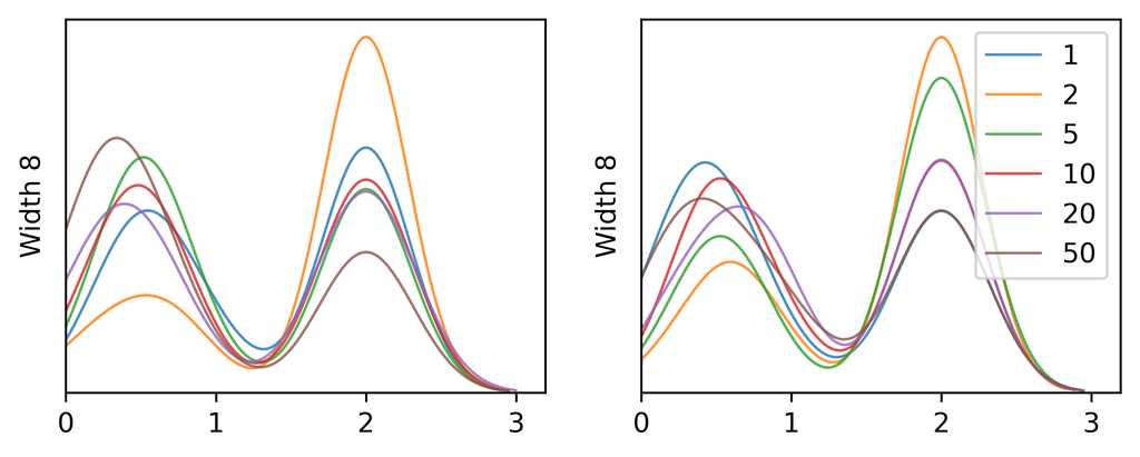
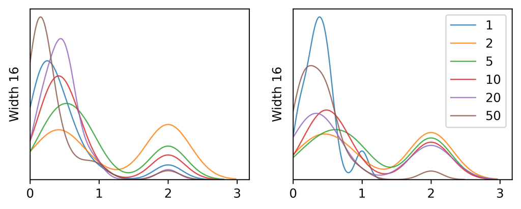
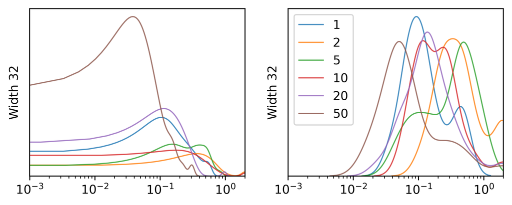
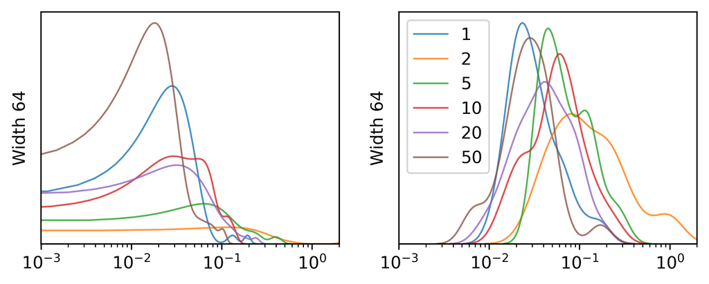
Figure 15: Distribution of average region volume (ARV) across training epochs, in the neighborhood of $25$ train (Left) and $25$ test (Right) samples from MNIST. We train an MLP with depth $5$ and vary its width between $\{8,16,32,16,128\}$. ARV is considerably large and bimodal for smaller widths; as network width is increased ARV becomes smaller and unimodal, with long smaller volume tails for training samples. This discrepancy between training and test samples, possibly indicates memorization.

Train                          Test

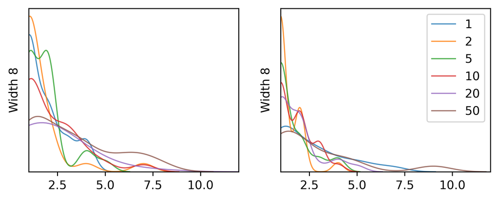
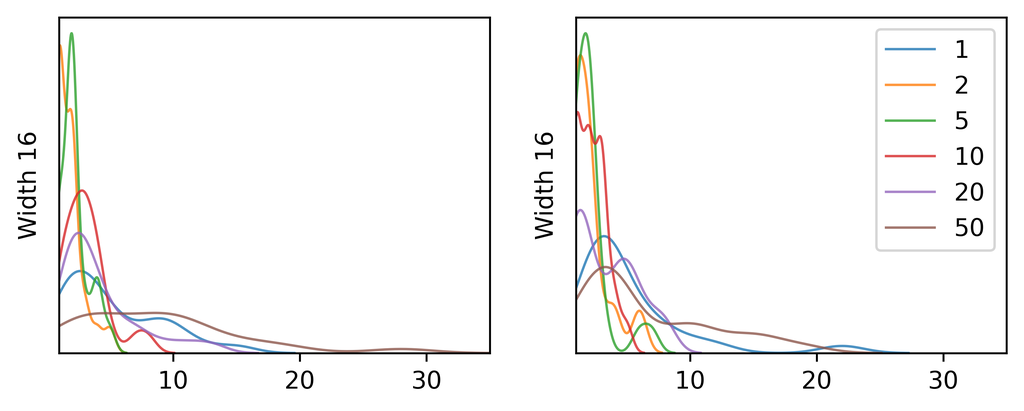
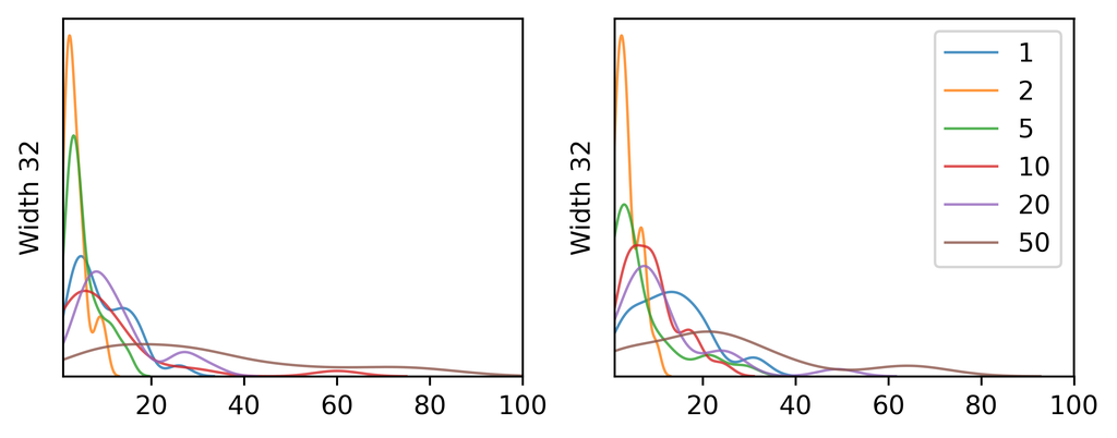
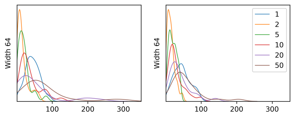
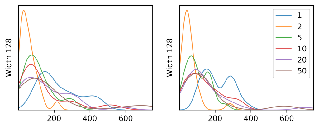
Figure 16: Distribution of average number of regions (ANR) across training epochs, in the neighborhood of $25$ train (Left) and $25$ test (Right) samples from MNIST. We train an MLP with depth $5$ and vary its width between $\{8,16,32,16,128\}$. ANR is small for smaller widths and increases significantly as the network width is increased. For larger networks, the distributions have large ANR tails. We can also see a shift towards lower ANR right after epoch 1 and a slow shift of the distribution towards larger ANR as training progresses.

Train                          Test

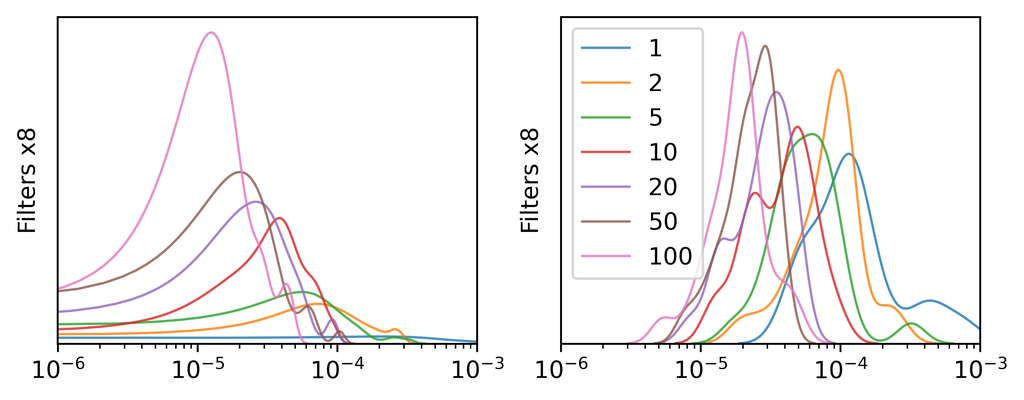
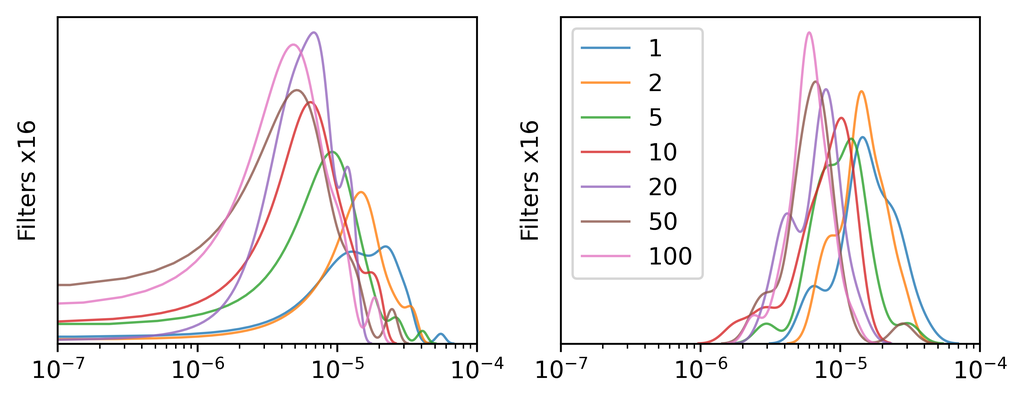
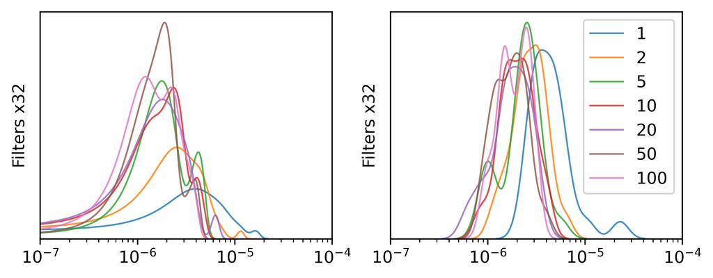
Figure 17: Distribution of average region volume (ARV) across training epochs, in the neighborhood of $25$ train (Left) and $25$ test (Right) samples from CIFAR10. We train a CNN with $6$ convolutional layers and $2$ fully connected layers. The number of filters for the layers are set as $\{\lfloor\ell/2\rfloor\times mul\ :\ell=1...6\}$, where $\lfloor.\rfloor$ is the floor operation, and $mul\in\{8,16,32\}$ is a width multiplier. We see that, similar to Fig. 15, the ARV gets reduced with increased width. For training, we can see longer tails towards lower ARV, indicating that for some training samples the regions become very small. For both train and test, with increasing number of epochs, the ARV distribution mean shifts towards lower ARV.

Train                          Test

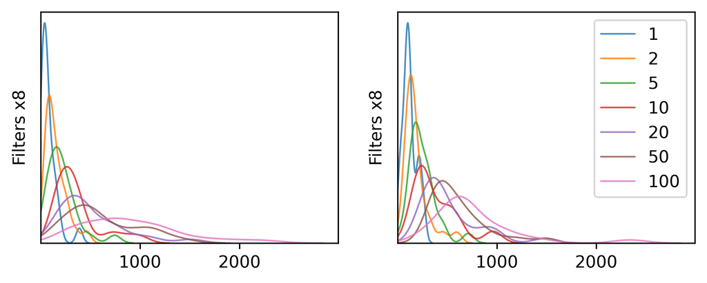
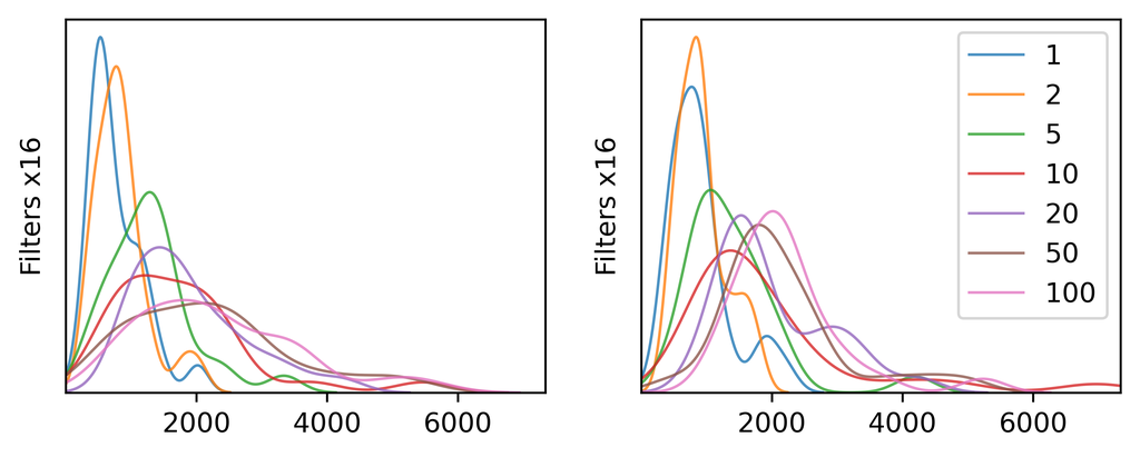
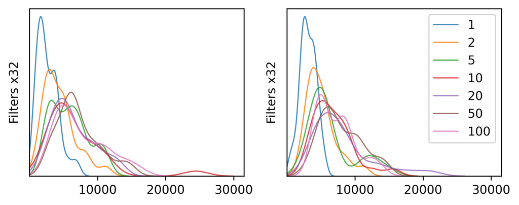
Figure 18: Distribution of average number of regions (ANR) across training epochs, in the neighborhood of $25$ train (Left) and $25$ test (Right) samples from CIFAR10. We train a CNN with $6$ convolutional layers and $2$ fully connected layers. The number of filters for the layers are set as $\{\lfloor\ell/2\rfloor\times mul\ :\ell=1...6\}$, where $\lfloor.\rfloor$ is the floor operation, and $mul\in\{8,16,32\}$ is a width multiplier. We see that, similar to Fig. 16, the ANR significantly increases with increased width. For training, we can see longer tails towards higher ANR, indicating that for some training samples there is high region density in the neighborhood. For both train and test, with increasing number of epochs, the ANR distribution mean shifts towards higher ANR.

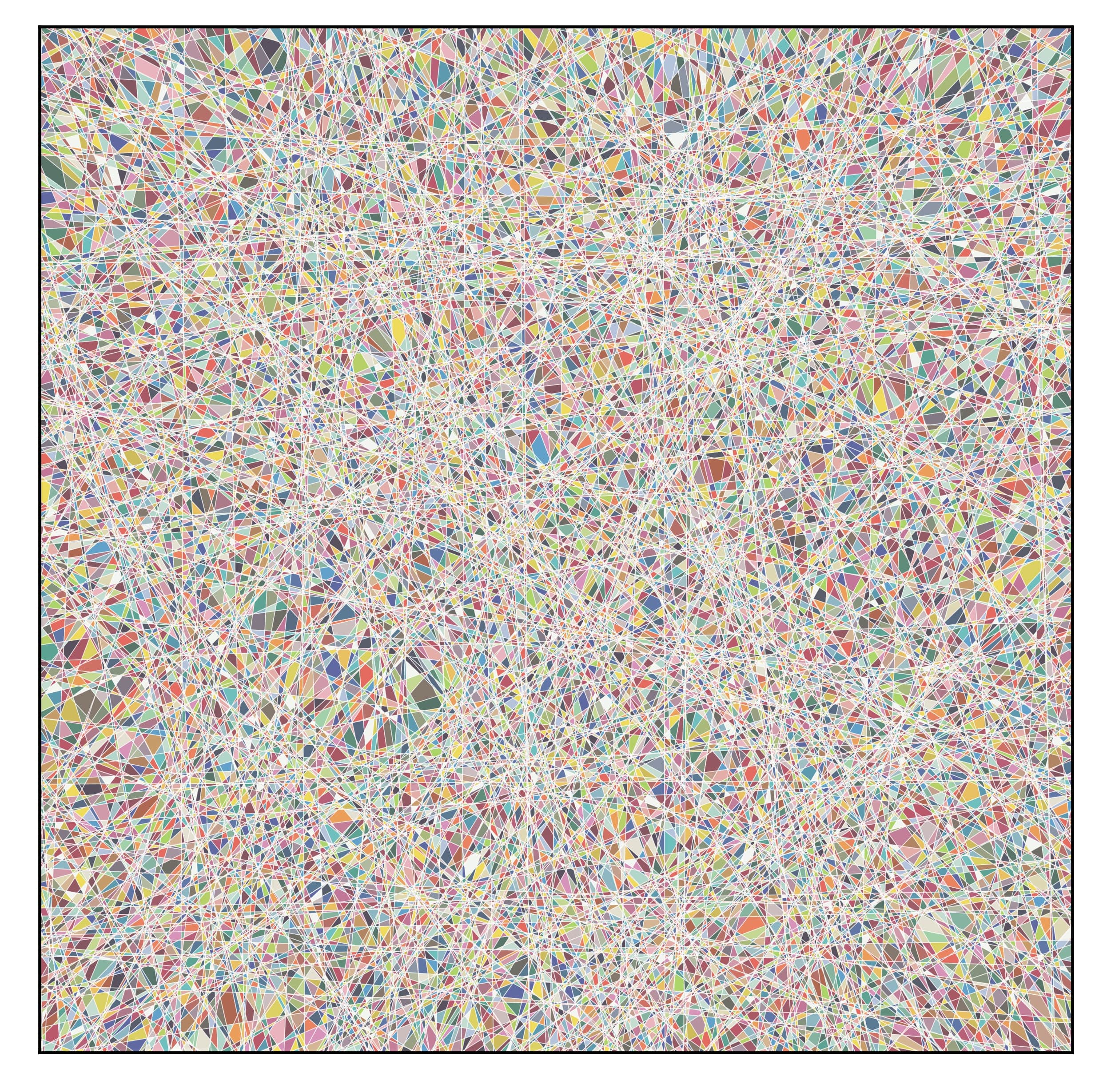
Figure 19: Partition visualization of a randomly initialized single layer MLP with 1000 hyperplanes and input dimensionality of 8002 for a randomly oriented 2D square domain centered on the origin. The partition contains $132569$ regions and takes $134s$ to compute.

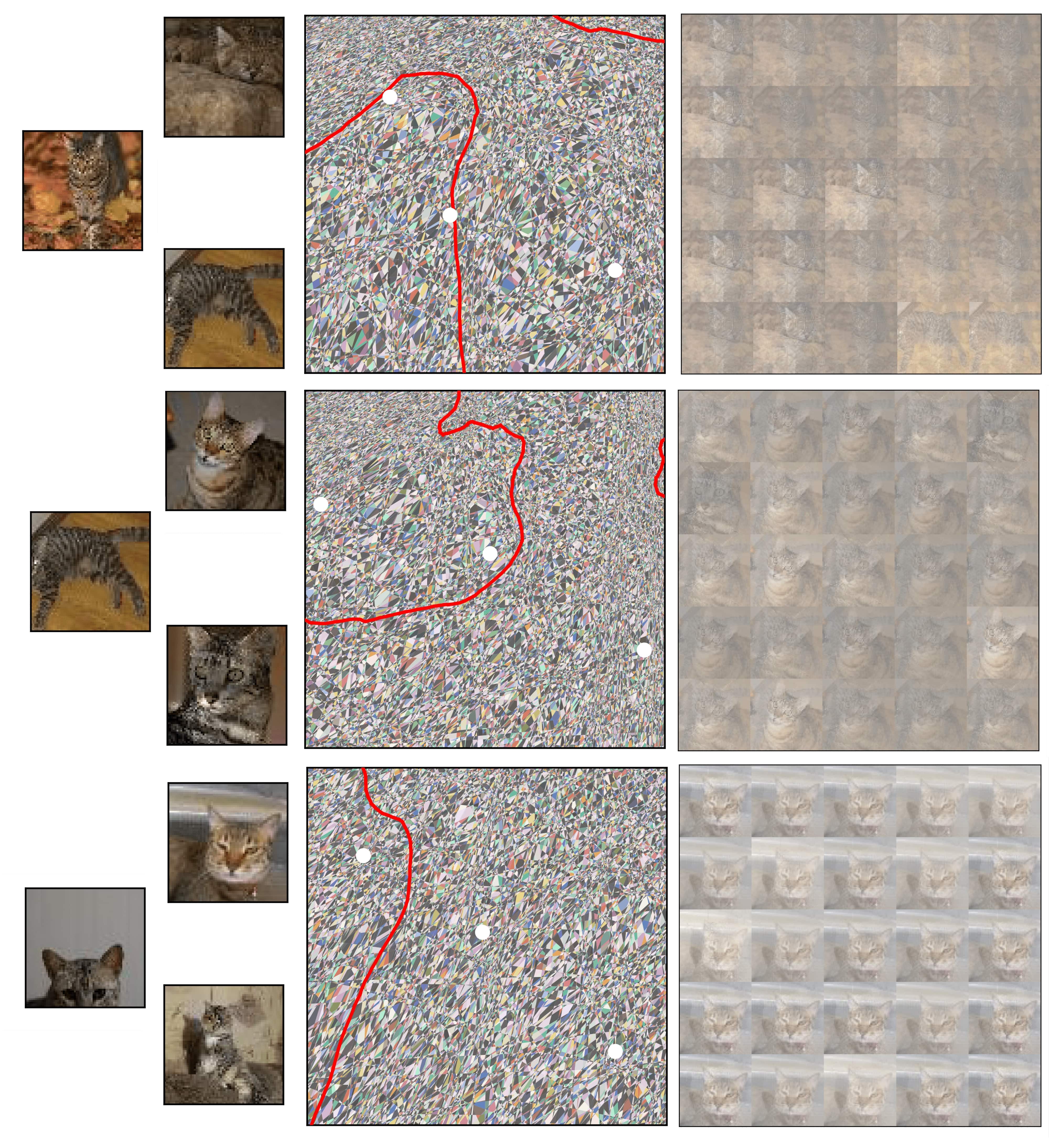
Figure 20: Partition visualization of a convolutional neural network, trained for binary classification of tinyimagenet Tabby Cat and Egyptian Cat classes. Left Samples that are used as anchor points to determine the 2D slice with an area of $450$ units. Middle The partitioning of input space induced by the model as well as the decision boundary (in red). Right Randomly sampled points from the decision boundary. Samples from the decision boundary visually represent a linear combination of the three anchor samples, while the weights are determined by the non-linear decision boundary. For example, for the top and bottom rows, samples from the boundary look biased towards two of the three anchor points. Computing the partition regions take 7.46 mins, 13.96 mins and 5.02 mins respectively, with each of the partitions containing 82817, 119895, and 60455 regions. The number of regions is positively correlated with the curvature of the decision boundary in the neighborhood.

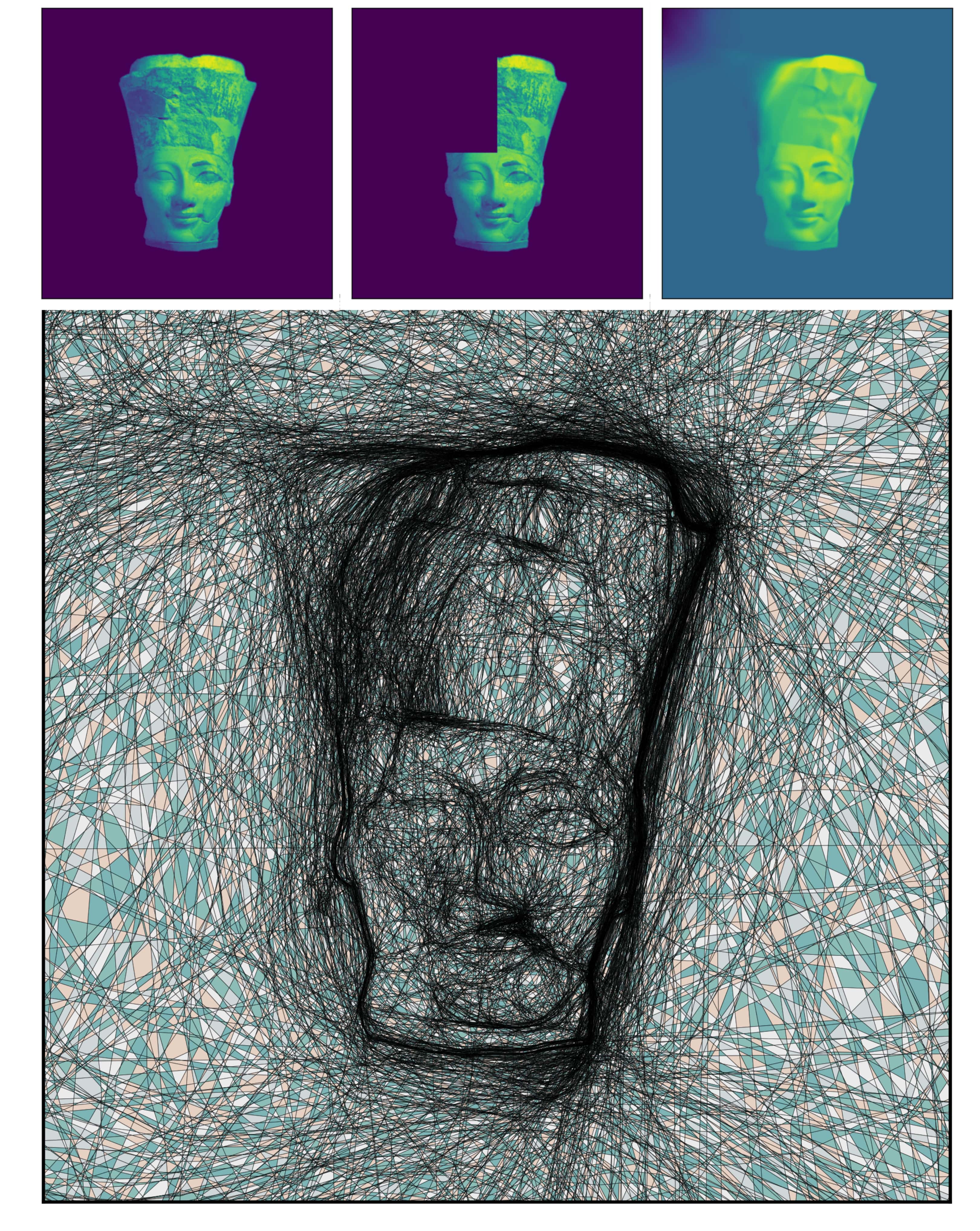
Figure 21: Training and visualizing the partition of a 2D INR trained on an inpainting task. Top row shows the original training image, the training image with a section cropped out and the predictions of a trained MLP with width 256 and depth 6. The MLP, via implicit regularization, learns a smooth surface in place of the discontinuity. Note how a lot of neurons are placed in the cropped region, and also around the foreground boundaries, to allow more curvature while fitting.

Appendix E Usage of SplineCam

We provide SplineCam as a python toolbox that can wrap any given Pytorch [30] sequential network, containing a set of supported modules. The toolbox is available for download in our anonymized Drive .zip file.

To begin, first we have to define a 2D input space region of interest (ROI). The region of interest is can be a polytopal region at the input of the network defined via vertices. Since all the region finding operations are performed in 2D, we also require an orthogonal projection matrix that projects vectors from the input space on to the 2D ROI. Following this we can use the SplineCam library to wrap a given model.

⬇

1

2import torch

3import splinecam

4

5## given torch model and domain (ROI) as a list of vertices

6

7T = splinecam.utils.get_proj_mat(domain)

8

9model.cuda()

10model.eval()

11model.type(torch.float64)

12

13print(’Wrapping model with SplineCam...’)

14NN = splinecam.wrappers.model_wrapper(

15 model,

16 input_shape=model.input_shape,

17 T = T,

18 dtype = torch.float64,

19 device = ’cuda’

20)

21

22## check .forward() and matmul operation equivalence

23print(’Verifying wrapped model...’)

24flag = NN.verify()

25print(’Model.forward and matmul equivalence check’, flag)

26assert flag

27

28#

Listing 1: Wrapping a model with splinecam

SplineCam supports custom layers as well. Each SplineCam layer requires a submodules to return the weights, the intersection pattern and activation pattern of the layer. We refer the reader to our codes for details. The wrapped SplineCam model contains a verification method, to ensure that the affine operations and the forward operations (which can be different from the affine operation based on implementation, e.g., convolution) of the model result in the same value for random inputs.

SplineCam can take any set of 2D domains as ROI, with corresponding projection matrices. This allows SplineCam to be used to visualize the partition for piecewise linear subspaces in the input space. The following example shows how SplineCam computes the partition in a layerwise fashion.

⬇

1

2## for a given list of polygons in 2D and corresponding projection matrices

3

4Abw = T

5out_cyc = poly

6

7for current_layer in range(1,len(NN.layers)):

8

9 ## given a set of 2D regions and a target layer, find all new regions in 2D

10 out_cyc,out_idx = splinecam.graph.to_next_layer_partition(

11 cycles = out_cyc,

12 Abw = Abw,

13 NN = NN,

14 current_layer = current_layer,

15 )

16

17 ## acquire region centroids

18 means = splinecam.utils.get_region_means(out_cyc)

19

20 ## pass each region centroid to next layer

21 means = NN.layers[:current_layer].forward(means)

22

23 ## get activation mask for each region

24 q = NN.layers[current_layer].get_activation_pattern(means)

25

26 ## query network weights

27 Wb = NN.layers[current_layer].get_weights()

28

29 ## calculate affine parameters per region

30 Abw = splinecam.utils.get_Abw(

31 q = q,

32 Wb = Wb.to_dense(),

33 incoming_Abw = Abw)

34

35#

Listing 2: Modular code for computing spline partition

One of the key algorithms in the to_next_layer_partition(.) function is the search algorithm that allows us to find cycles from a given graph. The following codeblock presents a pseudocode of our heuristic breadth first search method.

⬇

1

2from graph_tool import topology

3

4def find_cycles(V=input_graph,start_edge=input_edge):

5 ’’’

6 Given a undirected graph and a starting edge find cycles from that edge

7 ’’’

8

9 ## Convert V to a bidirectional graph. This allows us to control

10 ## the number of traversals for each edge

11 V = convert_to_bidirectional(V)

12 edge_q.append(start_edge)

13

14 ## if edge is a boundary edge

15 V.remove_edge(start_edge)

16

17 out_cycles = []

18

19 for e in edge_q:

20

21 remove_q = []

22 vertices = []

23 vertex_id = []

24

25 ## if no way out of v0 or no way in for v1, continue

26 if not (V.get_in_degrees(e.vertex1)>1

27 ) and (

28 V.get_out_degrees(e.vertex0)>1):

29 continue

30

31 ## if the edge doesn’t exist, continue

32 if V.edge(e) is None and V.edge(e.vertex1,e.vertex0) is None:

33 continue

34

35 ## add opposite path to removal queue

36 remove_q.append(V.edge(e.vertex1,

37 e.vertex0)))

38

39 ## bfs

40 vs,es = topology.shortest_path(V,

41 source=e.vertex0,

42 target=e.vertex1,

43 )

44

45 out_cycles.append([V.vertex_index[each] for each in vs])

46

47 for new_e in es:

48

49 ## if boundary edge remove edges in both directions

50 if V.ep[’layer’][new_e] == -1:

51 remove_q.append(new_e)

52 remove_q.append(V.edge(new_e.vertex1,new_e.vertex0))

53

54 else:

55 ## remove only one direction and append to queue

56 remove_q.append(new_e)

57 edge_q.append(new_e)

58

59 for each in remove_q:

60 V.remove_edge(each)

61

62 return out_cycles

Listing 3: Pseudocode function for finding cycles given a undirected graph

References

- [1] Pankaj K Agarwal. Partitioning arrangements of lines ii: Applications. Disc. & Comp. Geom., 1990.
- [2] R. Balestriero and R. G. Baraniuk. A spline theory of deep networks. In Proc. Int. Conf. Mach. Learn., volume 80, pages 374–383, Jul. 2018.
- [3] Randall Balestriero and Richard G Baraniuk. Batch normalization explained. arXiv preprint arXiv:2209.14778, 2022.
- [4] Randall Balestriero, Romain Cosentino, Behnaam Aazhang, and Richard Baraniuk. The geometry of deep networks: Power diagram subdivision. In Advances in Neural Information Processing Systems 32, pages 15806–15815, 2019.
- [5] Randall Balestriero, Ishan Misra, and Yann LeCun. A data-augmentation is worth a thousand samples: Exact quantification from analytical augmented sample moments, 2022.
- [6] Wuyang Chen, Xinyu Gong, and Zhangyang Wang. Neural architecture search on imagenet in four gpu hours: A theoretically inspired perspective. arXiv preprint arXiv:2102.11535, 2021.
- [7] Elliott Ward Cheney and William Allan Light. A course in approximation theory, volume 101. American Mathematical Soc., 2009.
- [8] Magnus Egerstedt and Clyde Martin. Control theoretic splines: optimal control, statistics, and path planning. Princeton University Press, 2009.
- [9] Cesare Fantuzzi, Silvio Simani, Sergio Beghelli, and Riccardo Rovatti. Identification of piecewise affine models in noisy environment. International Journal of Control, 75(18):1472–1485, 2002.
- [10] Alhussein Fawzi, Horst Samulowitz, Deepak Turaga, and Pascal Frossard. Adaptive data augmentation for image classification. In 2016 IEEE international conference on image processing (ICIP), pages 3688–3692. Ieee, 2016.
- [11] Matteo Gamba, Adrian Chmielewski-Anders, Josephine Sullivan, Hossein Azizpour, and Marten Bjorkman. Are all linear regions created equal? In International Conference on Artificial Intelligence and Statistics, pages 6573–6590. PMLR, 2022.
- [12] Amirata Ghorbani, Abubakar Abid, and James Zou. Interpretation of neural networks is fragile. In Proceedings of the AAAI conference on artificial intelligence, volume 33, pages 3681–3688, 2019.
- [13] Xavier Glorot, Antoine Bordes, and Yoshua Bengio. Deep sparse rectifier neural networks. In Proceedings of the fourteenth international conference on artificial intelligence and statistics, pages 315–323, 2011.
- [14] Boris Hanin and David Rolnick. Complexity of linear regions in deep networks. arXiv preprint arXiv:1901.09021, 2019.
- [15] L. A. Hannah and D. B. Dunson. Multivariate convex regression with adaptive partitioning. J. Mach. Learn. Res., 14(1):3261–3294, 2013.
- [16] Warren He, Bo Li, and Dawn Song. Decision boundary analysis of adversarial examples. In ICLR, 2018.
- [17] Alex Hernández-García and Peter König. Data augmentation instead of explicit regularization. arXiv preprint arXiv:1806.03852, 2018.
- [18] Ahmed Imtiaz Humayun, Randall Balestriero, and Richard Baraniuk. MaGNET: Uniform sampling from deep generative network manifolds without retraining. In International Conference on Learning Representations, 2022.
- [19] Ahmed Imtiaz Humayun, Randall Balestriero, and Richard Baraniuk. Polarity sampling: Quality and diversity control of pre-trained generative networks via singular values. In Proceedings of the IEEE/CVF Conference on Computer Vision and Pattern Recognition, pages 10641–10650, 2022.
- [20] Mohammad AAK Jalwana, Naveed Akhtar, Mohammed Bennamoun, and Ajmal Mian. Cameras: Enhanced resolution and sanity preserving class activation mapping for image saliency. In CVPR, pages 16327–16336, 2021.
- [21] Matt Jordan, Justin Lewis, and Alexandros G Dimakis. Provable certificates for adversarial examples: Fitting a ball in the union of polytopes. In Advances in Neural Information Processing Systems, 2019.
- [22] Tero Karras, Samuli Laine, Miika Aittala, Janne Hellsten, Jaakko Lehtinen, and Timo Aila. Analyzing and improving the image quality of stylegan. In Proc. CVPR, pages 8110–8119, 2020.
- [23] Yann LeCun, Yoshua Bengio, and Geoffrey Hinton. Deep learning. nature, 521(7553):436–444, 2015.
- [24] Andrea Locatelli, Alexandra Carpentier, and Samory Kpotufe. An adaptive strategy for active learning with smooth decision boundary. In Algorithmic Learning Theory, pages 547–571. PMLR, 2018.
- [25] A. Magnani and S. P. Boyd. Convex piecewise-linear fitting. Optim. Eng., 10(1):1–17, 2009.
- [26] Ben Mildenhall, Pratul P Srinivasan, Matthew Tancik, Jonathan T Barron, Ravi Ramamoorthi, and Ren Ng. Nerf: Representing scenes as neural radiance fields for view synthesis. In European conference on computer vision, pages 405–421. Springer, 2020.
- [27] Ben Mildenhall, Pratul P Srinivasan, Matthew Tancik, Jonathan T Barron, Ravi Ramamoorthi, and Ren Ng. Nerf: Representing scenes as neural radiance fields for view synthesis. Communications of the ACM, 65(1):99–106, 2021.
- [28] Guido F Montufar, Razvan Pascanu, Kyunghyun Cho, and Yoshua Bengio. On the number of linear regions of deep neural networks. In Advances in Neural Information Processing systems, pages 2924–2932, 2014.
- [29] Steven J Nowlan and Geoffrey E Hinton. Simplifying neural networks by soft weight-sharing. Neural computation, 4(4):473–493, 1992.
- [30] Adam Paszke, Sam Gross, Francisco Massa, Adam Lerer, James Bradbury, Gregory Chanan, Trevor Killeen, Zeming Lin, Natalia Gimelshein, Luca Antiga, Alban Desmaison, Andreas Kopf, Edward Yang, Zachary DeVito, Martin Raison, Alykhan Tejani, Sasank Chilamkurthy, Benoit Steiner, Lu Fang, Junjie Bai, and Soumith Chintala. Pytorch: An imperative style, high-performance deep learning library. In Advances in Neural Information Processing Systems 32, pages 8024–8035. Curran Associates, Inc., 2019.
- [31] Tiago P. Peixoto. The graph-tool python library. figshare, 2014.
- [32] Henning Petzka, Martin Trimmel, and Cristian Sminchisescu. Notes on the symmetries of 2-layer relu-networks. In Proceedings of the Northern Lights Deep Learning Workshop, volume 1, pages 6–6, 2020.
- [33] Mary Phuong and Christoph H. Lampert. Functional vs. parametric equivalence of re{lu} networks. In International Conference on Learning Representations, 2020.
- [34] Maithra Raghu, Ben Poole, Jon Kleinberg, Surya Ganguli, and Jascha Sohl-Dickstein. On the expressive power of deep neural networks. arXiv preprint arXiv:1606.05336, 2016.
- [35] Gowthami Somepalli, Liam Fowl, Arpit Bansal, Ping Yeh-Chiang, Yehuda Dar, Richard Baraniuk, Micah Goldblum, and Tom Goldstein. Can neural nets learn the same model twice? investigating reproducibility and double descent from the decision boundary perspective. In CVPR, pages 13699–13708, 2022.
- [36] Yu Sun, Jiaming Liu, Mingyang Xie, Brendt Wohlberg, and Ulugbek S Kamilov. Coil: Coordinate-based internal learning for imaging inverse problems. arXiv preprint arXiv:2102.05181, 2021.
- [37] Shuning Wang and Xusheng Sun. Generalization of hinging hyperplanes. IEEE Transactions on Information Theory, 51(12):4425–4431, 2005.
- [38] Yuan Wang. Estimation and comparison of linear regions for relu networks. In IJCAI, 2022.
- [39] Yulin Wang, Xuran Pan, Shiji Song, Hong Zhang, Gao Huang, and Cheng Wu. Implicit semantic data augmentation for deep networks. Advances in Neural Information Processing Systems, 32, 2019.
- [40] Jason Yosinski, Jeff Clune, Anh Nguyen, Thomas Fuchs, and Hod Lipson. Understanding neural networks through deep visualization. ICML Deep Learning Workshop, page 12, 2015.
- [41] Gizem Yüce, Guillermo Ortiz-Jiménez, Beril Besbinar, and Pascal Frossard. A structured dictionary perspective on implicit neural representations. In Proceedings of the IEEE/CVF Conference on Computer Vision and Pattern Recognition, pages 19228–19238, 2022.
- [42] Xiao Zhang and Dongrui Wu. Empirical studies on the properties of linear regions in deep neural networks. arXiv preprint arXiv:2001.01072, 2020.