LISA Galactic binaries with astrometry from Gaia DR3

Abstract

Galactic compact binaries with orbital periods shorter than a few hours emit detectable gravitational waves at low frequencies. Their gravitational wave signals can be detected with the future Laser Interferometer Space Antenna (LISA). Crucially, they may be useful in the early months of the mission operation in helping to validate LISA’s performance in comparison to pre-launch expectations. We present an updated list of 55 candidate LISA detectable binaries with measured properties, for which we derive distances based on Gaia Data release 3 astrometry. Based on the known properties from EM observations, we predict the LISA detectability after 1, 3, 6, and 48 months using Bayesian analysis methods. We distinguish between verification and detectable binaries as being detectable after 3 and 48  months respectively. We find 18 verification binaries and 22 detectable sources, which triples the number of known LISA binaries over the last few years. These include detached double white dwarfs, AM CVn binaries, one ultracompact X-ray binary and two hot subdwarf binaries. We find that across this sample the gravitational wave amplitude is expected to be measured to $\approx 10\%$ on average, while the inclination is expected to be determined with $\approx 15^{\circ}$ precision. For detectable binaries these average errors increase to $\approx 50\%$ and to $\approx 40^{\circ}$ respectively.

1 Introduction

Binary systems composed of degenerate stellar remnants (white dwarfs, neutron stars and black holes) in orbits with periods of less than a few hours are predicted to be strong gravitational wave (GW) sources in our own Galaxy. A number of these systems – primarily consisting of a neutron star or white dwarf paired with a compact helium-star, white dwarf, or another neutron star – have been identified primarily through the observation in optical and X-ray electromagnetic (EM) wavebands. Some of these systems display remarkably short orbital periods, down to just several minutes (e.g. Amaro-Seoane et al., 2023). Binaries in a such a tight orbit emit GWs at mHz frequencies that can be detected directly with the future Laser Interferometer Space Antenna (LISA, Amaro-Seoane et al., 2017), and other future planned space-based GW observatories such as TianQin (Luo et al., 2016; Huang et al., 2020), Taiji (Ruan et al., 2018) and the Lunar Gravitational Wave Antenna (Harms et al., 2021).

In this study we focus on the LISA mission, which is a European Space Agency (ESA)-led GW observatory currently scheduled for launch in the mid-2030s. Designed to operate in the frequency band between $0.1$ mHz and $100$ mHz (Amaro-Seoane et al., 2017), LISA is an ideal tool for discovering massive black hole mergers and extreme-/intermediate-mass ratio inspirals. In addition, it can survey the shortest period stellar remnant binaries throughout the entire Milky Way, providing a complementary view of our Galaxy to EM surveys (for a review see Amaro-Seoane et al., 2023). Both theory- and observation-based studies find that LISA will deliver a sample of ${\cal O}(10^{4})$ binaries with orbital periods of $<1$ hour, which will be complete up to periods of $<15\,$min (e.g. Nelemans et al., 2001; Ruiter et al., 2009; Nissanke et al., 2012; Lamberts et al., 2019; Breivik et al., 2020; Li et al., 2020; Korol et al., 2022). A significant number of ${\cal O}(10^{2})$ of stellar remnant binaries – primarily those composed of two white dwarfs – discovered by LISA will be possible to study in combination with EM surveys (e.g. Nelemans et al., 2004; Marsh, 2011; Korol et al., 2017; Breivik et al., 2018; Tauris, 2018; Li et al., 2020).

In the context of the LISA mission, stellar remnant binaries known from EM observations are often termed ‘verification binaries’, based on the idea that one can model their GW signal using EM measurements of binary’s parameters and to employ these to test LISA data quality (e.g. Ströer & Vecchio, 2006; Littenberg, 2018; Savalle et al., 2022). In our previous work, we reviewed a sample of candidate LISA verification binaries following the second Gaia data release (DR2). This allowed us to determine distances – previously highly uncertain for most binaries – based on Gaia’s parallax measurements (Kupfer et al., 2018; Ramsay et al., 2018). In turn, new distance estimates enabled us to evaluate the uncertainty on the expected GW signal’s amplitude and to assess the detectability of these candidate verification binaries with LISA. In this work we update the sample of candidates LISA verification binaries in a number of ways. Firstly, we include several newly discovered systems since Gaia DR2 (Section 2). Secondly, we re-evaluate the distances based on improved astrometry from the third Gaia DR3, while also taking into account their proper motion information (Section 3.3). In addition, we evaluate their detectability as well as the binary parameter estimation in a fully-Bayesian way using the up-to-date LISA sensitivity requirements (Section 3.4).

So far verification binaries have been (arbitrarily) defined as such based on an assumed signal-to-noise ratio (SNR) detection threshold reached at a set observation time. However, this definition relies on a few caveats. Firstly, the SNR threshold and the integration time needed to make an unambiguous identification of a (known) source is not just a matter of source’s intrinsic amplitude, but is also heavily dependent on the realization of the rest of the Galactic population (i.e. unresolved Galactic confusion foreground) that the source is competing against (e.g. figure 4 of Korol et al., 2023). In addition, the Galactic confusion foreground is dynamic: it will decrease with time as more and more sources will become detectable and will become individually resolved. Moreover, LISA’s orbit around the Sun will introduce a modulation in the Galactic foreground reaching its maximum when LISA is optimally oriented towards the Galactic center, which is where the density of Galactic sources peaks (e.g. Petiteau, 2008). A prototype global fit data analysis pipeline for LISA demonstrated that the Galactic foreground subtraction steadily improves with time with a few ${\cal O}(10^{3})$ binaries being identified (and subtracted) already after 1 month (Littenberg & Cornish, 2023). Moreover, known binaries will be the most crucial in the early weeks/months of the mission operation in helping to validate the early performance of the instrument in comparison to pre-launch expectations. It is therefore reasonable to expect that the first data validation may be required after only a few months from the beginning of science operations. We anticipate that an integration time as short as 1-3 months would allow for basic consistency tests on the recovered parameters on a few epochs of commissioning data for several verification binaries. Given all the above, in this study we opt to call as verification binary a system that becomes detectable, which is judged based on the shape of the recovered posteriors on binary’s parameters rather than a SNR threshold, within 3 months of observation time with LISA, and we call a as detectable binary when it is detected after 48 months (at present set as the nominal lifetime of the mission).

2 The sample of compact LISA sources since Gaia DR2

At present the catalog of candidate verification binaries includes detached (Brown et al., 2016a) and semi-detached double white dwarfs (the latter called AM CVn type binaries; see Solheim (2010) for a recent review), hot subdwarf stars with a white dwarf companion (see Geier et al. (2013); Kupfer et al. (2022); Pelisoli et al. (2021) for recent discoveries), semi-detached white dwarf-neutron star binaries (so-called ultracompact X-ray binaries; Nelemans & Jonker 2010), double neutron stars (Lyne et al., 2004) and Cataclysmic Variables (CVs, Scaringi et al., 2023). In Kupfer et al. (2018) we analyzed $\sim 50$ known candidates using distances derived from parallaxes provided in the Gaia DR2 catalog (DR2, Gaia Collaboration et al., 2018). We found that 13 candidates exceed a SNR threshold of 5 for a LISA mission duration of 4 years.

The Zwicky Transient Facility (ZTF) performed a dedicated high-cadence survey to find short period binaries (Kupfer et al., 2021). More than 20 new binary systems with orbital periods ranging from 7 min to $\approx 1$ h have been discovered by ZTF since the beginning of science operations in March 2018 (Bellm, 2014; Burdge et al., 2019a, 2020a, 2020b; Kupfer et al., 2020a, b; van Roestel et al., 2022; Burdge et al., 2023). This new sample includes eight eclipsing systems, seven AM CVn systems, and six systems exhibiting primarily ellipsoidal variations in their light curves. Remarkably, one of the first ZTF discoveries was the shortest orbital period detached eclipsing binary system known to date, ZTF J1539+5027, with an period of just 6.91 min (Burdge et al., 2019a). Owing both to its inherently high GW frequency and large GW amplitude, ZTF J1539+5027 is expected to be one of the loudest Galactic GW sources and could reach the SNR detection threshold of $\approx 7$ within a week. Littenberg & Cornish (2019) showed that for high frequency systems like ZTF J1539+5027, GW measurements will independently provide comparable levels of precision to the current EM measurement of the orbital evolution of the system, and will improve the precision to which the distance and orientation is known.

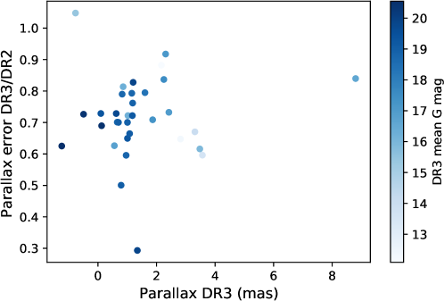
Figure 1: The error of the parallax in DR3 compared to DR2 for the verification sources in Tables 1 and 2. The color indicates the mean $G$ mag of the source.

The Extremely Low Mass (ELM) White Dwarf Survey has successfully completed its observations across the footprint of the Sloan Digital Sky Survey (SDSS), and expanded their search to the Southern hemisphere (Brown et al., 2022; Kosakowski et al., 2020, 2023a). Over the last few years the ELM survey discovered several sub-hour orbital-period double degenerates, including the first double helium-core white dwarf binary (e.g. Brown et al. 2020; Kilic et al. 2021; Kosakowski et al. 2021, 2023b). It is expected that double helium-core white dwarfs and carbon/oxygen + helium-core white dwarfs dominate the population in the LISA band despite that they make up only 10% of the global double white dwarf population (Lamberts et al., 2019).

Moreover, several additional candidates have been found in other large-scale surveys. SDSS J1337 was discovered as a double degenerate in early SDSS-V data with an orbital period of 99 min. The spectrum shows spectral lines from both components making it a double lined system which provides precise system parameters (Chandra et al., 2021). Pelisoli et al. (2021) discovered a compact hot subdwarf binary with a massive white dwarf companion in a 99 min period orbit in the TESS sky survey. The total mass of the system is above the Chandrasekhar mass making the system a double degenerate supernova Ia progenitor. Scaringi et al. (2023) showed that three known CVs, namely WZ Sge, VW Hyi and EX Hya, could be individually resolved after four years of LISA operation.

Since the release of Gaia DR2 a few years ago, numerous sky surveys have collectively tripled the number of identified candidate compact binaries. It’s noteworthy, however, that these surveys employ a variety of detection techniques and analysis methods, leading to heterogeneity in the presentation of results. Table 1 offers an overview of the observational results for known sources detectable by LISA, as reported in the respective studies. The properties of all sources compiled for this publication are accessible to the public via the LISA Consortium’s GitLab repository at https://gitlab.in2p3.fr/LISA/lisa-verification-binaries.

Table 1: Physical properties of the known verification and detectable binaries. Masses and inclination angles in brackets are assumed and based on evolutionary stage and mass ratio estimations. Absolute magnitudes are calculated from the Gaia $G$-band magnitude in combination with our distance estimate.

Source	Type	Orbital	$l_{\rm Gal}$	$b_{\rm Gal}$	BP-RP	$M_{\textrm{G}}$	$m_{\rm 1}$	$m_{\rm 2}$	$\iota$
		period (s)	(deg)	(deg)	(mag)	(mag)	(M⊙)	(M⊙)	($\deg$)
Verification binaries
HM Cnc1,2	AMCVn	321.529129(10)	206.9246	23.3952	$0.246$	6.54	0.55	0.27	$\approx$38
ZTFJ15393	DWD∗	414.7915404(29)	80.7746	50.5819	$-0.263$	8.44	$0.61^{+0.017}_{-0.022}$	$0.21\pm 0.015$	$84.15^{+0.64}_{-0.57}$
ZTFJ22434	DWD∗	527.934890(32)	104.1514	–5.4496	$-0.160$	9.33	$0.349^{+0.093}_{-0.074}$	$0.384^{+0.114}_{-0.074}$	$81.88^{+1.31}_{-0.69}$
V407 Vul5	AMCVn	569.396230(126)	57.7281	6.4006	$1.535$	7.76	[0.8$\pm$0.1]	[0.177$\pm$0.071]	[60]
ES Cet6	AMCVn∗	620.21125(30)	168.9684	–65.8632	$-0.296$	5.55	[0.8$\pm$0.1]	[0.161$\pm$0.064]	[60]
SDSSJ0651∗7,8	DWD∗	765.206543(55)	186.9277	12.6886	$0.029$	9.37	0.247$\pm$0.015	0.49$\pm$0.02	${86.9^{+1.6}_{-1.0}}$
ZTFJ05389	DWD∗	866.60331(16)	186.8104	–6.2213	$0.025$	8.80	$0.45\pm 0.05$	$0.32\pm 0.03$	$85.43^{+0.07}_{-0.09}$
SDSSJ135110	AMCVn	939.0(7.2)	328.5021	53.1240	$-0.122$	7.80	[0.8$\pm$0.1]	[0.100$\pm$0.040]	[60]
AM CVn11,12	AMCVn	1028.7322(3)	140.2343	78.9382	$-0.283$	6.66	0.68$\pm$0.06	0.125$\pm$0.012	43$\pm$2
ZTFJ19059	AMCVn∗	1032.16441(62)	0.1945	1.0968	$-0.066$	11.47	[0.8$\pm$0.1]	[0.090$\pm$0.035]	$70\pm 20$
SDSSJ190813,14	AMCVn	1085.108(1)	70.6664	13.9349	$-0.018$	6.27	[0.8$\pm$0.1]	[0.085$\pm$0.034]	10 - 20
HP Lib15,16	AMCVn	1102.70(5)	352.0561	32.5467	$-0.153$	6.36	0.49-0.80	0.048-0.088	26-34
SDSSJ093517,18	DWD	1188(42)	176.0796	47.3776	$0.455$	9.82	0.312$\pm$0.019	0.75$\pm$0.24	[60]
J0526+593419	DWD	1230.37467(7)	151.9201	13.2614	$0.186$	7.92	$0.378^{+0.066}_{-0.060}$	$0.887^{+0.110}_{-0.098}$	$57.1^{+4.3}_{-4.1}$
J1239-204120	DWD	1350.432(11.232)	299.2755	42.0943	$-0.072$	9.00	$0.291\pm 0.013$	${0.68^{+0.11}_{-0.06}}$	${71^{+8}_{-10}}$
TIC378898110	AMCVn	1347.96	297.0555	1.9451	0.027	6.82	[0.8$\pm$0.1]	[0.10$\pm$0.02]	$74\pm 10$
CR Boo16,21	AMCVn	1471.3056(500)	340.9671	66.4884	$0.066$	7.74	0.67-1.10	0.044-0.088	30
SDSS063422	DWD	1591.4(28.9)	176.7322	13.3211	$-0.189$	8.95	${0.452^{+0.070}_{-0.062}}$	${0.209^{+0.034}_{-0.021}}$	$37\pm 7$
V803 Cen16,23	AMCVn	1596.4(1.2)	309.3671	20.7262	$0.232$	8.44	0.78-1.17	0.059-0.109	12 - 15
Detectable binaries
4U1820–3024,25	UCXB	685(4)	2.7896	–7.9144	-	3.745	[1.4]	[0.069]	[60]
ZTFJ012726	DWD∗	822.680314(43)	128.4671	–9.5102	. $0.191$	9.26	$0.75\pm 0.06$	$0.19\pm 0.03$	[75-90]
SDSSJ232227	DWD	1201.4(5.9)	85.9507	–51.2104	$-0.179$	9.08	$0.34\pm 0.02$	$>0.17$	[60]
PTFJ053328	DWD	1233.97298(17)	201.8012	–16.2238	$-0.067$	8.70	$0.652^{+0.037}_{-0.040}$	$0.167\pm 0.030$	$72.8^{+0.8}_{-1.4}$
ZTFJ20299	DWD∗	1252.056499(41)	58.5836	–13.4655	$-0.054$	10.27	$0.32\pm 0.04$	$0.30\pm 0.04$	$86.64^{+0.70}_{-0.40}$
PTF1J191929	AMCVn∗	1347.354(20)	79.5945	15.5977	$0.036$	9.08	[0.8$\pm$0.1]	[0.066$\pm$0.026]	[60]
TIC37889811030	AMCVn	1347.96	297.0555	1.9451	$0.027$	6.82	[0.8$\pm$0.1]	[0.1$\pm$0.02]	$74\pm 10$
CXOGBSJ175131	AMCVn	1374.0(6)	359.9849	–1.4108	$1.623$	6.01	[0.8$\pm$0.1]	[0.064$\pm$0.026]	[60]
ZTFJ07229	DWD∗	1422.548655(71)	232.9930	–1.8604	$-0.157$	8.23	$0.38\pm 0.04$	$0.33\pm 0.03$	$89.66\pm 0.22$
KL Dra32	AMCVn	1501.806(30)	91.0140	19.1992	$0.668$	9.25	0.76	0.057	[60]
PTF1J071933	AMCVn	1606.2(1.2)	168.6573	24.4945	$0.425$	9.30	[0.8$\pm$0.1]	[0.053$\pm$0.021]	[60]
CP Eri34,35	AMCVn	1740(84)	191.7021	–52.9098	$0.218$	10.5	[0.8$\pm$0.1]	[0.049$\pm$0.020]	[60]
SMSSJ033821	DWD	1836.1(31.9)	128.8576	20.7792	$-0.129$	8.64	$0.230\pm 0.015$	$0.38^{+0.05}_{-0.03}$	$69\pm 9$
J2322+210320	DWD	1918.08(21.60)	96.5151	–37.1844	$0.071$	8.81	$0.291\pm 0.013$	$0.75\pm 0.26$	[60]
SDSSJ010636	DWD	2345.76(1.73)	191.9169	31.9952	$-0.223$	10.30	$0.188\pm 0.011$	$0.57^{+0.22}_{-0.07}$	$67\pm 13$
SDSSJ163037	DWD	2388.0(6.0)	67.0760	43.3604	$-0.147$	9.54	0.298$\pm$0.019	0.76$\pm$0.24	[60]
J1526m271138	DWD	2417.645(37.930)	340.4437	24.1935	$-0.108$	9.36	$0.37\pm 0.02$	$>0.40\pm 0.02$	[60]
SDSSJ123539,40	DWD	2970.432(4.320)	284.5186	78.0320	$-0.219$	9.27	$0.35\pm 0.01$	$0.27^{+0.06}_{-0.02}$	$27.0\pm 3.8$
SDSSJ092341	DWD	3883.68(43.20)	195.8199	44.7754	$-0.236$	8.62	0.275$\pm$0.015	0.76$\pm$0.23	[60]
CD–30∘1122342	sdB∗	4231.791855(155)	322.4875	28.9379	$-0.388$	4.55	0.54$\pm$0.02	0.79$\pm$0.01	82.9$\pm$0.4
SDSSJ133743	DWD	5942.952(300)	89.0428	74.0799	$0.306$	11.31	$0.51\pm 0.01$	$0.32\pm 0.01$	$13\pm 1$
HD26543544	sdB	5945.917432(280)	87.0170	1.1225	$-0.425$	3.76	$0.63^{+0.13}_{-0.12}$	$1.01\pm 0.15$	$64^{+14}_{-5}$

[1]Strohmayer (2005), [2]Roelofs et al. (2010), [3]Burdge et al. 2019a, [4]Burdge et al. 2020b, [5]Ramsay et al. (2002), [6]Espaillat et al. (2005), [7]Brown et al. (2011), [8]Hermes et al. (2012), [9]Burdge et al. 2020a, [10]Green et al. (2018), [11]Skillman et al. (1999), [12]Roelofs et al. (2006), [13]Fontaine et al. (2011), [14]Kupfer et al. (2015), [15]Patterson et al. (2002) , [16]Roelofs et al. (2007), [17]Brown et al. (2016b), [18]Kilic et al. (2014), [19]Kosakowski et al. (2023b), [20]Brown et al. (2022), [21]Provencal et al. (1997), [22]Kilic et al. (2021), [23]Anderson et al. (2005), [24]Stella et al. (1987), [25]Chen et al. (2020), [26]Burdge et al. (2023), [27]Brown et al. (2020), [28]Burdge et al. (2019b), [29]Levitan et al. (2014), [30]Green et al. (2024), [31]Wevers et al. (2016) [32]Wood et al. (2002), [33]Levitan et al. (2011), [34]Howell et al. (1991), [35]Groot et al. (2001), [36]Kilic et al. (2011b), [37]Kilic et al. (2011a), [38]Kosakowski et al. (2023a), [39]Kilic et al. (2017), [40]Breedt et al. (2017), [41]Brown et al. (2010), [42]Geier et al. (2013), [43]Chandra et al. (2021), [44]Pelisoli et al. (2021), [45] $M_{V}$ taken from van Paradijs & McClintock (1994)

3 Methods

3.1 Improvements from Gaia DR2 to Gaia DR3

In 2018 Gaia DR2 released full astrometric solutions, including parallaxes, and proper motions for 1.3 billion sources (Gaia Collaboration et al., 2016, 2018). The release was based on observations taken between July 2014 and May 2016. The parallaxes allowed us for the first time to calculate distances for a large sample of LISA detectable compact binaries. The distances in combination with the chirp mass provided the opportunity to calculate GW amplitudes and estimate the detectability for LISA (Kupfer et al., 2018). Until Gaia DR2 only a small sample of AM CVn binaries had parallax measurements using the Hubble Space telescope (Roelofs et al., 2007).

About two years after the second data release, the Gaia early data release (eDR3) provided full astrometric solutions for 1.4 billion sources based on 34 month of observations (Gaia Collaboration et al., 2020). The released data included one additional year of Gaia data leading to a higher precision in the parallaxes and proper motions compared to DR2 as well as first time parallax measurements for several LISA sources, including ZTFJ1905, ZTFJ0127, SDSSJ0935, V803 Cen and CR Boo. Generally, we find that the parallaxes improved by about 20% - 30% between DR2 and eDR3, in particular for faint sources (Fig. 1). Our list also contains six binaries with either a negative parallax or a parallax error close to $100\%$. These are ZTF J1539, ZTF J2243, V407 Vul, ZTF J1905, 4U 1830-30, and ZTF J2029. We anticipate that for these objects the distance estimate is dominated by the derived scale length prior (cf. Section 3.3). We note that distances can also be estimated through indirect methods. In particular spectroscopic distances have been used for double white dwarfs. For this work we only include parallaxes to derive distances to be independent from spectroscopic models.

In June 2022 Gaia data release 3 (DR3) was released. Gaia DR3 included the same data as eDR3 and as such astrometric solutions did not improve between eDR3 and DR3. However, DR3 included a large amount of additional information, including orbital astrometric solutions for wide binaries with a clean solution (Gaia Collaboration et al., 2022). For the remainder of the paper we will always refer to DR3 knowing that parallaxes and proper motions are the same for eDR3 and DR3.

3.2 Systems with uncertain parallax or alternative distance estimates

Here, we take the opportunity to discuss a few systems with uncertain parallax or alternative distance estimates: HM Cnc, 4U 1830$-$30, V407 Vul, and ZTF J1905.

HM Cnc is the only remaining system with no parallax measurement. Therefore, the distance estimate of HM Cnc remains debated. Roelofs et al. (2010) estimated a distance of 5 kpc based on its properties whereas Reinsch et al. (2007) estimated a distance of $\approx$2 kpc based on the observed flux. Most recently Munday et al. (2023) presented the discovery of $\ddot{f}=(-5.38\pm 2.10)\times 10^{-27}$Hz s^-2 in HM Cnc. They concluded that HM Cnc is close to the period minimum and theoretical MESA calculations find a mass of $\approx$1 M_⊙  for the accretor and $\approx$0.17 M_⊙ for the donor. This result is in strong contradiction to the results presented in Roelofs et al. (2010) based on a spectroscopic analysis. Munday et al. (2023) also discussed different ways to measure the distance to HM Cnc and found values between 2 kpc and 11 kpc. This shows the very large uncertainties of the system properties from EM studies. As a consequence, the expected GW amplitude also remains uncertain.

In practice, 4U 1830$-$30 also lacks a parallax measurement. However, it is located in the globular cluster NGC 6624, which allows for an independent distance estimate using color-magnitude diagrams with theoretical isochrones, or by using variable stars that follow known relations between their periods and absolute luminosities like RR Lyrae stars. NGC 6624 has a well-measured distance of $7972\pm 277$ pc (Baumgardt & Vasiliev, 2021), which we take as the distance for 4U 1830$-$30.

V407 Vul’s optical counterpart is dominated by a component that matches a G-type star with a blue variable (Steeghs et al., 2006). It is still unknown whether this is a chance alignment or whether V407 Vul is a triple system where an ultracompact inner binary is orbited by a G-star companion. Companions in orbits with a multi-year orbital period can present themselves in Gaia DR3 data, either they are listed in the non-single star tables of Gaia DR3 (nss_two_body_orbit) or they have a non-zero value in the astrometric_excess_noise keyword in the gaia_source table. The latter is non-zero if the astrometric solution shows additional perturbations to a single-source solution which could be an indication of a astrometric wobble if the G-star in V407 Vul is in a wide orbit (e.g. Belokurov et al., 2020; Penoyre et al., 2020). V407 Vul is not listed in the non-single star tables of Gaia DR3 (nss_two_body_orbit) and has an astrometric_excess_noise=0 and astrometric_excess_noise_sig=0 and therefore there is no indication in the current Gaia DR3 data set that the G-star is a wide companion to the inner ultracompact binary. However, we note that Gaia DR3 is only sensitive to few years periods. Longer periods would not yet show up as astrometric wobble and therefore we cannot exclude that the G-star has a period of more than a few years.

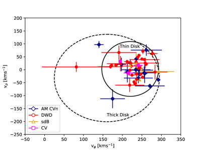
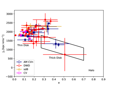
Figure 2: $V_{\phi}$–$V_{\rho}$ (left) and $e$–$J_{z}$ diagrams (right). The solid and dotted ellipses render the 3$\sigma$ thin and thick disk contours in the $V_{\phi}$–$V_{\rho}$ diagram, while the solid box in the $e$–$J_{z}$ marks the thick disk region as specified by Pauli et al. (2006)

ZTF J1905 presents a particular challenge with its uncertain Gaia DR3 parallax ($\varpi=1.8652\pm 1.5428$). This parallax value would imply the system’s absolute magnitude of $\approx 11$ mag, which seems contradictory when compared to AM CVn binaries with similar orbital periods such as AM CVn or SDSS J1908. Typically, AM CVn systems in the orbital period range between 15 min - 20 min are much brighter, characterized by absolute magnitudes around 6.5 mag. There is no indication in the Gaia DR3 quality keywords that the parallax is problematic. Additionally, there is only modest extinction towards the direction of ZTF J1905. Green et al. (2019) reports $E(g-r)=0.18$ which results in an extinction of $\approx$0.5 mag in the Gaia$-G$ band, which is not sufficient to explain the apparent discrepancy. The distance of ZTF J1905 thus needs further investigation.

3.3 Distance estimation

Gaia DR3 provides parallaxes which can be used to determine distances. To estimate distances from the measured parallaxes we use a probability-based inference approach (e.g. Bailer-Jones, 2015; Igoshev et al., 2016; Astraatmadja & Bailer-Jones, 2016; Bailer-Jones et al., 2018; Luri et al., 2018; Bailer-Jones et al., 2021). We follow a similar approach as described in detail in Sec. 3.2 in Kupfer et al. (2018). The measured parallax follows a probability distribution and with a prior on the true distance distribution for the observed sources we can constrain the distance even if the parallax has large uncertainties. If the parallax uncertainty is below $10$% - $20$% the distance estimate is independent of the prior. At larger uncertainties on the distance, the distance estimate becomes more and more dependent on the prior. We apply Bayes’ theorem to measure the probability density for the distance:

$$P(r|\varpi,\sigma_{\varpi})=\frac{1}{Z}\ P(\varpi|d,\sigma_{\varpi})\ P(d),$$ (1)

where $d$ is the distance, $P(\varpi|r,\sigma_{\varpi})$ is the likelihood function, that can be assumed Gaussian (Lindegren et al., 2018). $P(r)$ is the prior and $Z$ is a normalization constant. As in Kupfer et al. (2018) we adopt an exponentially decreasing volume density prior $P(d)$

$$P(d)=\begin{cases}\frac{d^{2}}{2L^{3}}\exp(-d/L)&\text{if}\ d>0\\ 0&\text{otherwise},\end{cases}$$ (2)

where $L>0$ is the scale length. Compared to our previous study, here we assume two values for $L$ based on the binary’s membership to the thin or thick disc as detailed below. We also stress that for systems with poor parallax measurement, the distance estimate largely depends on our assumption for $L$.

To estimate if our candidate LISA binaries are members of the thin or thick disc, for each binary we calculate Galactic kinematics, i.e. velocity components and Galactic orbit. To do this, sky position, proper motions, systemic velocities, and distances are needed. We extract proper motions from Gaia DR3 and calculate the distance using Eqs. (1) and (2) by setting $L=400$ pc or $L=795$ pc; these are typical values for $L$ for thin disc and thick disc objects respectively. Additionally, we use published systemic velocities, typically from radial velocity measurements. For systems with unknown systemic velocities, we assume $1$ km s${}^{-1}\pm 50$ km s^-1. As for the distance estimate, we calculate Galactic kinematics assuming $L$ values of 400 pc (thin discs) and 795 pc (thick disc). Using the Galactic potential of Allen & Santillan (1991) as revised by Irrgang et al. (2013), we calculate velocity in the direction of the Galactic center ($V_{\rho}$) and the Galactic rotation direction ($V_{\phi}$), the Galactic orbital eccentricity ($e$), and the angular momentum in the Galactic $z$ direction ($J_{z}$). The Galactic radial velocity $V_{\rho}$ is negative towards the Galactic center, while stars that are revolving on retrograde orbits around the Galactic center have negative $V_{\phi}$. Stars on retrograde orbits have positive $J_{z}$. Thin disk stars generally have very low eccentricities $e$. Population membership can be derived from the position in the $V_{\rho}$ - $V_{\phi}$ diagram and the $J_{z}$ - $e$ diagram (Pauli et al., 2003, 2006). We find that for all objects the population membership is independent of the assumption for $L$ and we apply the appropriate value for $L$ for the distance estimation. Fig. 2 shows the population memberships for our candidate LISA sources. Most systems can be identified as thin disc objects. Table 2 presents the calculated distances with the assigned value for $L$.

Table 2: Measured EM properties (parallax, distance) and derived GW parameters of the verification binaries and detectable binaries. The distance for HM Cnc is assumed. The fractional error for the amplitude ($\sigma_{\mathcal{A}}/\mathcal{A}$) and the precision the inclination ($\Delta\iota$) is calculated for four years integration with LISA.

Source	$f$	$\varpi$ DR3a	$\varpi$ DR2a	$L$	$d$	$\sigma_{\mathcal{A}}/\mathcal{A}$	$\Delta\iota$
	(mHz)	(mas)	(mas)	(pc)	(pc)	(%)	(deg)
Verification binaries
HM Cnc	6.220	-	-		[5000 – 10,000]	9.5	21
ZTFJ1539	4.822	$-0.4926\pm 0.5726$	$-0.1125\pm 0.7884$	795	$2469\pm 1253$	1.1	0.6
ZTFJ2243	3.788	$-1.2372\pm 0.6578$	$-1.5658\pm 1.0522$	400	$1756\pm 726$	$0.36$	0.6
V407 Vul	3.512	$0.0978\pm 0.2384$	$0.0949\pm 0.3272$	400	$2089\pm 684$	2.0	1.9
ES Cet	3.225	$0.5606\pm 0.0677$	$0.5961\pm 0.1081$	795	$1779\pm 234$	2.2	2.1
SDSSJ0651	2.614	$1.0071\pm 0.3091$	$1.0002\pm 0.4759$	400	$958\pm 370$	1.8	0.9
ZTFJ0538	2.308	$0.9617\pm 0.2866$	$1.1477\pm 0.4811$	400	$999\pm 366$	2.8	1.5
SDSSJ1351	2.130	$0.6584\pm 0.2197$	$0.5957\pm 0.3134$	795	$1530\pm 755$	27.9	33
AM CVn	1.944	$3.3106\pm 0.0303$	$3.3512\pm 0.0452$	795	$302\pm 3$	12.5	23
ZTFJ1905	1.938	$1.8652\pm 1.5428$	-	400	$697\pm 605$	11.6	35
SDSSJ1908	1.843	$1.0232\pm 0.0335$	$0.9542\pm 0.0464$	400	$977\pm 32$	19.5	30
HP Lib	1.814	$3.5674\pm 0.0313$	$3.6225\pm 0.0525$	400	$280\pm 3$	13.3	24
SDSSJ0935	1.683	$2.7034\pm 0.6648$	-	400	$395\pm 203$	3.3	3.1
J0526+5934	1.625	$1.1826\pm 0.0910$	$1.1294\pm 0.1097$	400	$845\pm 68$	18.0	9.6
J1239-2041	1.481	$1.0068\pm 0.2309$	$1.4054\pm 0.3297$	400	$972\pm 272$	13.3	9.5
TIC378898110	1.483	$3.2328\pm 0.0195$	$3.2186\pm 0.0307$	400	$309\pm 2$
CR Boo	1.359	$2.8438\pm 0.0367$	-	400	$351\pm 5$	19.8	29
SDSSJ0634	1.257	$2.3111\pm 0.0835$	$2.3578\pm 0.091$	400	$433\pm 16$	19.4	28
V803 Cen	1.253	$3.4885\pm 0.0599$	-	400	$287\pm 5$	16.1	27
Detectable binaries
4U 1820$-$30	2.920	$-0.7676\pm 0.2164$	$-0.8199\pm 0.2065$	-	$7972\pm 277^{c}$	32.3	34
ZTFJ0127	2.431	$0.4438\pm 0.4657$	-	400	$1283\pm 603$	7.2	2.4
SDSSJ2322	1.665	$1.1558\pm 0.2244$	$1.2869\pm 0.2830$	400	$859\pm 206$	29.6	36
PTFJ0533	1.621	$0.7902\pm 0.2396$	$0.4741\pm 0.4786$	400	$1173\pm 390$	33.3	30
ZTFJ2029	1.597	$0.1240\pm 0.9893$	$-1.4269\pm 1.4345$	400	$1095\pm 644$	$18.4$	10
PTF1J1919	1.484	$0.6229\pm 0.2385$	$0.5499\pm 0.3274$	400	$1364\pm 471$	65.2	46
TIC378898110	1.484	$3.2328\pm 0.0195$	$3.2186\pm 0.0307$	400	$309\pm 2$	19.0	6.5
CXOGBSJ1751	1.456	$0.8591\pm 0.1733$	$0.4994\pm 0.2130$	400	$1128\pm 258$	48.4	41
ZTFJ0722	1.406	$0.6996\pm 0.2457$	$0.4132\pm 0.3508$	795	$1461\pm 785$	46.3	23
KL Dra	1.332	$1.0817\pm 0.0989$	$1.0354\pm 0.1488$	795	$930\pm 91$	65.4	49
PTF1J0719	1.245	$1.1851\pm 0.2292$	$1.1436\pm 0.3009$	400	$840\pm 201$	68.0	48
CP Eri	1.149	$1.3451\pm 0.2759$	$0.6836\pm 0.9407$	400	$747\pm 203$	82.6	55
SMSSJ0338	1.089	$1.8675\pm 0.0562$	$1.8994\pm 0.0793$	400	$536\pm 16$	43.2	40
J2322+2103	1.043	$0.8261\pm 0.2503$	$0.6943\pm 0.3168$	400	$1134\pm 386$	38.1	38
SDSSJ0106	0.853	$1.2011\pm 0.4739$	$1.3521\pm 0.5726$	400	$824\pm 441$	76.7	51
SDSSJ1630	0.837	$1.1748\pm 0.1952$	$0.9366\pm 0.2704$	400	$848\pm 167$	40.1	39
J1526m2711	0.827	$1.6053\pm 0.1751$	$1.5683\pm 0.2203$	400	$625\pm 75$	39.8	38
SDSSJ1235	0.673	$2.2504\pm 0.1389$	$2.3319\pm 0.1660$	400	$446\pm 28$	39.8	38
SDSSJ0923	0.515	$3.4795\pm 0.0648$	$3.3397\pm 0.1052$	400	$288\pm 5$	41.3	38
CD–30∘11223	0.473	$2.8198\pm 0.0516$	$2.9629\pm 0.0797$	400	$355\pm 7$	67.8	46
SDSSJ1337	0.337	$8.8007\pm 0.0440$	$8.6993\pm 0.0524$	400	$114\pm 1$	32.1	35
HD265435	0.336	$2.1666\pm 0.0554$	$2.1994\pm 0.0628$	400	$461\pm 12$	70.6	54

^aGaia Collaboration et al. (2018), ^bGaia Collaboration et al. (2020), ^cBaumgardt & Vasiliev (2021)

3.4 Gravitational wave parameter estimation

Gravitational radiation for a typical stellar remnant binary at mHz frequencies can be modeled as a quasi-monochromatic signal characterized by 8 parameters: GW frequency $f$, heliocentric amplitude ${\cal A}$, frequency derivative $\dot{f}$, sky coordinates $(\lambda,\beta)$, inclination angle $\iota$, polarization angle $\psi$, and initial phase $\phi_{0}$. The GW frequency and amplitude are given by

$$f=2/P_{\rm orb},$$ (3)

with $P_{\rm orb}$ being the binary’s orbital period, and

$$\mathcal{A}=\frac{2(G\mathcal{M})^{5/3}}{c^{4}d}(\pi f)^{2/3}.$$ (4)

This is set by the binary’s distance $d$ and chirp mass

$$\mathcal{M}=\frac{(m_{1}m_{2})^{3/5}}{(m_{1}+m_{2})^{1/5}},$$ (5)

for component masses $m_{1}$ and $m_{2}$. The frequency derivative $\dot{f}$ is expected to follow the gravitational radiation equation:

$$\dot{f}=\frac{96}{5}\frac{(G\mathcal{M})^{5/3}}{\pi c^{5}}(\pi f)^{11/3}.$$ (6)

To forecast LISA observations of the known binaries we use the vbmcmc sampler in ldasoft (Littenberg et al., 2020). The sampler uses a parallel tempered Markov Chain Monte Carlo algorithm with delta-function priors on the orbital period and sky location of the binary based on the EM observations (cf. Table 1). The priors on the remaining parameters are uniform in log amplitude and cosine inclination with the start value for the inclination being set to the measured values for systems with constraints on the inclination and set to 60 deg for unconstrained systems. The sampler is also marginalizing over the first time derivative of the frequency, polarization angle, and initial phase of the binary, all of which are considered nuisance parameters for this study. Because this is a targeted analysis of known binaries the trans-dimensional sampling capabilities in ldasoft are disabled and the algorithm uses a single template to recover the signal – effectively a delta function prior on the model. In this configuration, results for binaries below the detection threshold are used to set upper limits on the GW amplitude parameter.

The data being analyzed are simulated internally by vbmcmc and include stationary Gaussian noise with the same instrument noise spectrum as was used for the LISA Data Challenges (LDCs) in Challenge 2a plus an estimated astrophysical foreground from the unresolved Galactic binaries as described in Cornish & Robson (2017). The analysis ignores any correlations, contamination, or additional statistical uncertainty caused by the presence of other signals in the data, and also treats the astrophysical foreground as a stationary noise source. Relaxing these simplifying assumptions will be most relevant for binaries where the astrophysical foreground dominates the instrument noise spectrum at GW frequencies ${\lesssim}3$ mHz but is currently beyond the scope of this analysis (considering overlap with other sources) or capabilities of the sampling algorithm (considering non-stationary noise).

4 Results

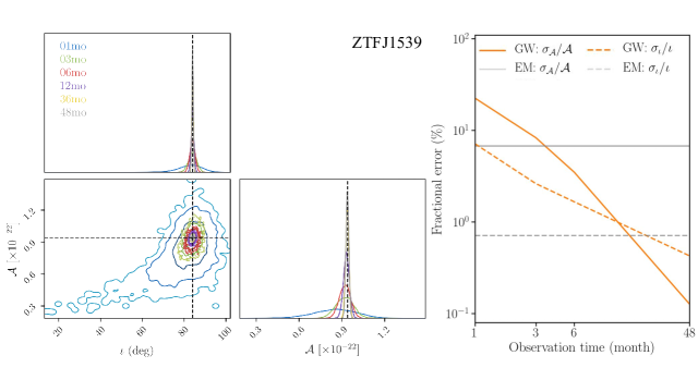
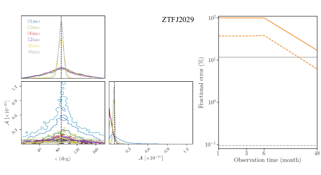
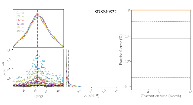
Figure 3: Three examples of posteriors for binary’s inclination and GW amplitude; from top to bottom these are: ZTFJ1539 (verification binary), ZTFJ2029 (detectable binary) and SDSSJ0822 (non-detectable binary). On the left we show how the estimated fractional error on the amplitude $\sigma_{\cal A}/{\cal A}$ and inclination $\sigma_{\iota}/\iota$ change as the functions of observation time; for comparison we also show current EM constrains and assuming that these won’t change before LISA’s launch (cf. Table 1 and 2).

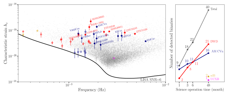
Figure 4: Left panel: Characteristic strain - frequency plot for detectable and verification binaries: AM CVns in blue, DWDs in red, sdBs in yellow and UCXB in magenta. Filled stars represent binaries detectable within 3 month of observations, which we call here ‘verification binaries’. The error bars on characteristic strain show $1\sigma$ uncertainty evaluated by generating random samples from EM measurement uncertainties on binary component masses and distances presented in Table 1 and 2. Black solid line represents LISA’s sensitivity curve that accounts for the instrumental noise (LISA Science Study Team, 2018) and Galactic confusion foreground (Babak et al., 2017). For comparison in gray we show a mock Galactic DWD population detectable with LISA from Wilhelm et al. (2021). Right panel: Number of detected binaries as a function of science operation time.

We analyze 55 verification binary candidates in total using the vbmcmc sampler in ldasoft for increasingly longer LISA mission science operation time: 1, 3, 6, 12, 36 and 48 months. We remind the reader that we perform a “targeted” analysis by fixing – using delta-function priors – binary’s sky position and orbital period to the values provided by EM measurements; additionally, we marginalize over $\dot{f}$, $\psi$ and $\phi_{0}$ (cf. Section 3.4). Differently from our previous work to assess the detectability of a binary, instead of evaluating the SNR we look at the binary’s GW parameters posterior samples. We consider the binary as detectable if the GW amplitude parameter is constrained away from the minimum value allowed by the prior. This is most readily identifiable by looking at the two dimensional posterior distribution in the GW amplitude-inclination plane, where a detectable binary will have closed contours in the posterior. We call as verification binary a system that becomes detectable (as explained in Sec. 1) within 3 months of observation time with LISA and we call as detectable binary when it is detected after 48 months of observation time with LISA. We introduce this distinction to highlight the use of verification binaries for the early data validations, e.g. in preparation for the first data release.

Our results show that an integration time as short as 1-3 months would allow for basic consistency tests on the recovered parameters on a few epochs of commissioning data for 9-18 verification binaries; while extending our definition up to 6 month increases the sample by only four additional binaries. To clarify the difference between a verification, detectable and non-detectable binary, in Fig. 3 we show posteriors of the binary’s inclination and GW amplitude for three examples: ZTFJ1539 ($\sim 7\,$min orbital period, verification binary), ZTFJ2029 ($\sim 21\,$min, detectable binary) and SDSSJ0822 ($\sim 40$ min, non-detectable binary). ZTFJ1539 shows closed contours already after 1 month of observations, which become increasingly narrow as observation time increases. Being detectable so early on, it is highly likely that ZTFJ1539 can be used as one of LISA’s verification binary. ZTFJ2029 represents an intermediate case as initially its posterior contours are open at low amplitude, but they close after 36 months at which point we classify this binary as detectable. Finally, we show the case of SDSSJ0822 which, based on the same reasoning as above, we classify as non detectable. Right panels of Fig. 3 illustrate how LISA’s fractional error on GW amplitude ${\cal A}$ and inclination $\iota$ (orange lines) improve over time. Assuming that EM measurement would not improve in the future, which is plausible if no additional EM measurements are taken between now and when LISA will fly, we show the estimate of the same parameters based on the current EM measurement (gray lines) for comparison.

Based on our definition above, overall we find 40 binaries detectable with LISA within 4 yr of science operations, out of which we classify 18 (10 AM CVns + 8 DWDs) as verification binaries, i.e. detectable within the first 3 months. We list their properties in Table 1 and 2. The summary of our results is presented in Fig. 4. In the left panel we show characteristic strain - frequency plot for all detectable binaries: AM CVns in blue, DWDs in red, sdBs in yellow and UCXB in magenta. Filled stars represent LISA verification binaries, empty stars are detectable binaries within the nominal mission life time (48 month). We compute the error bars on characteristic strain by generating random samples from EM measurement uncertainties on binary component masses and distance (cf. Table 1 and 2); in the figure we plot $1\sigma$ uncertainty based on our random samples. For comparison we also show a mock Galactic DWD population of Wilhelm et al. (2021) in gray, as well as the LISA sensitivity curve at SNR=6 as black solid line. The comparison reveals that the current sample of known binaries is mainly representative of the ‘loudest’ GW sources in the Milky Way, while the majority is yet to be discovered in more remote parts of our Galaxy inaccessible for EM observatories (see figure 15 of Amaro-Seoane et al., 2023). In the right panel of Fig. 4 we show the detection statistic as a function of the science operation time with a break down for different types of binaries showing that in increased science operation for LISA will lead to a larger number of detected binaries in the LISA data. We note that in our study none of the CVs will be detectable within four years of LISA observations.

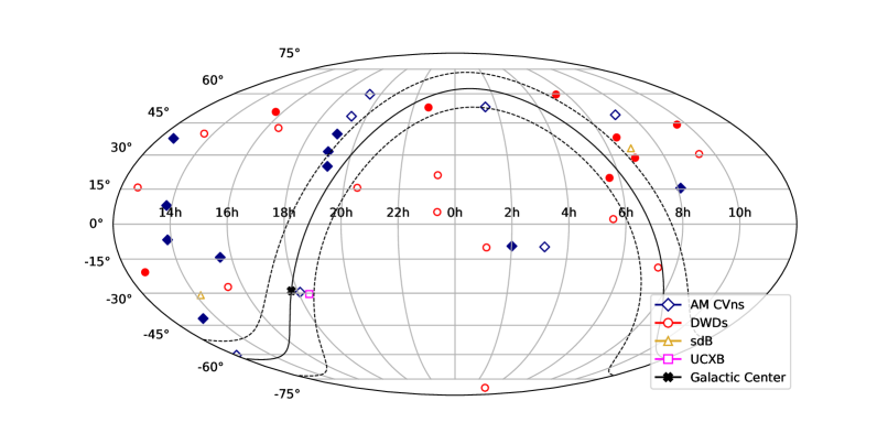
Figure 5: The position of the LISA binaries on the sky in an equatorial projection, with the Galactic plane ($\pm 10^{\circ}$) shown by the full and dashed lines. Filled symbols are verification binaries whereas open symbols are detectable binaries.

In our previous study Kupfer et al. (2018), we identified 13 detectable binaries. The reasons for the difference are multiple. Firstly, the sample of candidate verification binaries has tripled in the past few years (cf. Section 2). Secondly, some distance estimates have improved between Gaia DR2 and DR3 (this is, for example, true for CXOGBSJ1751 and SDSSJ163); for some binaries (ZTFJ0127, ZTFJ1905, SDSSJ0935, V803 Cen, CR Boo) parallaxes were not available as part of the DR2. Most importantly, we also change our criterion for the detectability moving away from a SNR based definition. Recently, Finch et al. (2023) have used our catalog for a number of LISA data analysis investigations by performing a Bayesian parameter estimation with the Balrog code (Roebber et al., 2020; Buscicchio et al., 2021; Klein et al., 2022). They verified that binaries with SNR$<$6 generally display broad posteriors, with no clear peaks and with amplitude parameter being inconsistent with zero. Thus, they adopted the SNR threshold of 6 as criterion for the detectability with LISA. They found that up to 14 binaries can be detected within 3 months of observations (see their figures 4 and B1). This result is in agreement with ours considering new binaries that have been added to the list of candidates in our study.

We report estimated fractional error on the GW amplitude ($\sigma_{\cal A}/{\cal A}$) and the estimated precision for the inclination ($\Delta\iota$) that can be reached after 4 years of observation in Table 2. On average, for verification binaries the amplitude is forecasted to be measured to $\sim 10$%, while the inclination is expected to be determined with $\sim 15^{\circ}$ precision. For detectable binaries these average errors decrease to $\sim 50$% and to $\sim 40^{\circ}$ respectively. From the table one can deduce that the measurements depend on the binary’s frequency (generally improving with increasing frequency) and strength of the signal (with verification binaries being better characterized than detectable binaries). Our estimates are in good agreement with Finch et al. (2023, see their table 2).

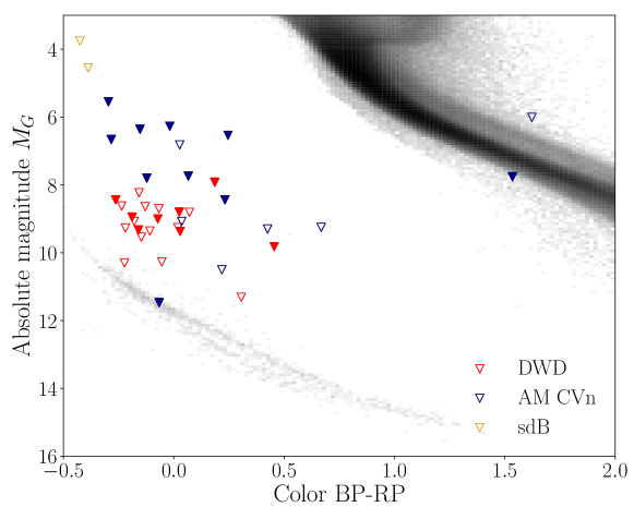
Figure 6: Verification binaries (in color) on the Gaia Hertzsprung-Russell diagram (in gray). Down-pointing triangles are used to symbolize that absolute magnitude estimates are to be interpreted as upper limits because we do not account for extinction. As before, filled symbols represent verification binaries whereas open symbols represent detectable binaries.

Figures 5 and 6 illustrate respectively the position of detectable (empty symbols) and verification (filled symbols) binaries on the sky and on the Gaia Hertzsprung-Russell (HR) diagram. Both reveal different limitations of the current sample. Figure 5 shows that although the size of the candidate LISA binaries is progressively growing, it is still biased towards the Northern Hemisphere (where the majority of surveys have been conducted so far), and to high latitudes (to avoid the dust extinction and crowding in the Galactic plane). From observations of bright non-degenerate stars we know that the Galactic stellar population is concentrated in the disc (region in between dashed lines) peaking towards the Galactic center (thick black cross in Fig. 5), and so we expect LISA detectable binaries to follow the same distribution (e.g. see Szekerczes et al., 2023). Figure 6 shows our sample of LISA sources compared to the absolute magnitudes ($M_{G}$) and colors ($BP-RP$) of Gaia’s sample of stars with parallax uncertainty below 1% (gray points). The plot shows a bias towards sources brighter and bluer compared to objects on the white dwarf track where most DWDs are expected. We note that on the HR diagram we use down-pointing triangles to highlight that our absolute magnitude estimates in our sample are to be interpreted as upper limits. This is because for all candidate LISA binaries the extinction, which is necessary to convert apparent $G$ magnitudes measured by Gaia magnitudes into absolute magnitudes $M_{G}$, is not well measured. Potential LISA sources with larger magnitudes can only be observed up to a couple kpc with current surveys, which limits the volume where LISA binaries can be detected. In contrast to EM searches, LISA measures directly the amplitude of GW waves, rather than the energy flux. Thus, the observed GW signal scales as $1/d$, rather than $1/d^{2}$, allowing LISA to detect binaries at larger distances – potentially within the entire Milky Way volume – than in the traditional EM observational bands.

5 Discussion

5.1 Limitations of the current sample and prospects to expand the sample

The currently known sample of candidate LISA verification binaries is inhomogeneous and biased. This bias is evident in the sky distribution (Fig. 5), predominantly favoring the Northern hemisphere with $60$% of LISA sources. Furthermore, the HR diagram (Fig. 6) reveals an over-representation of sources above the main white dwarf track. This is due to the nature of magnitude-limited ground-based surveys favoring brighter sources. Finally, a significant challenge lies in the multitude of detection and analysis methods, leading to a non-uniformity in presenting parameters of these binaries. Parameters are presented in varied ways: with a $1-\sigma$ error, no constraints, approximations or limits. To facilitate more effective future multi-messenger studies, it is essential to develop uniform analysis methods that provide a standard set of prior information.

Between Gaia DR2 and Gaia DR3 the number of detectable LISA sources has tripled which can be explained by the large number of sky surveys that came online over the last few years. This will improve even more over the next decade with many additional surveys coming online over the next few years. As proven in the past, photometric and spectroscopic surveys are ideal tools to find new LISA binaries and complement each other. Eclipses or tidal deformation lead to photometric variability on the orbital period, whereas compact LISA binaries show up in multi-epoch spectroscopy due to large radial velocity shifts between individual spectra.

SDSS-V is an all-sky, multi-epoch spectroscopic survey which started operations in 2020 and will provide spectra for a few million sources (Kollmeier et al., 2017). Already in early SDSS-V data Chandra et al. (2021) discovered a new detectable LISA binary. Other spectroscopic ongoing or upcoming spectroscopic surveys include LAMOST (Zhao et al., 2012), 4MOST (de Jong et al., 2019) or WEAVE (Dalton et al., 2014). The Asteroid Terrestrial-impact Last Alert System (ATLAS, Tonry et al., 2018; Heinze et al., 2018) and the Gravitational-wave Optical Transient Observer (GOTO, Steeghs et al., 2022) are ongoing photometric sky surveys with telescopes located in both hemispheres allowing for an all-sky coverage for both surveys. Their cadence and sky coverage are well suited to find LISA detectable binaries. BlackGEM is a photometric sky survey covering the Southern hemisphere which has started operations in 2023 (Bloemen et al., 2015). Part of the BlackGEM operations will be the BlackGEM Fast Synoptic Survey which is a continuous high cadence survey of individual fields in the Southern hemisphere. The cadence is ideal to discover new LISA detectable binaries. First light for the Vera Rubin telescope is expected in 2024. The telescope will perform the Legacy Survey of Space and Time (LSST) covering the Southern hemisphere down to 24 mag (per single exposure) going much deeper and hence covering a significantly larger volume than current sky surveys. Although the cadence is expected to be not ideal for LISA binaries, LSST will collect sufficient photometric observations over 10 years to be able to discover LISA binaries. The next large Gaia data release (DR4) is expected to include precision time series photometry of $\approx$70 epochs for each object taken over a five year time frame. Euclid is a space mission operating in the near-infrared and visible bands which was launched in 2023 with an unprecedented sky resolution of almost one order of magnitude better compared to ground based observatories. Part of Euclid’s operation will be the Euclid deep survey covering a total of 40 sqd for three distinct fields. Each field will get several tens of epochs over its nominal mission time of six years with a depth of $\approx 25$ mag for each epoch in the near-infrared bands (Laureijs et al., 2011). Finally, in the late 2020s the Nancy Roman space telescope will conduct a wide-field survey with the same sky resolution as Euclid down to 24 mag. Therefore, we expect that the number of LISA detectable sources will significantly increase before the LISA launches providing a large sample of multi-messenger sources (e.g. Korol et al., 2017; Li et al., 2020).

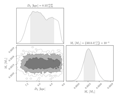
Figure 7: Posterior distribution for HM Cnc’s expected chirp mass and distance precision predicted for four years of LISA observations.

5.2 Focus for future EM efforts

EM measurement of a binary’s inclination will significantly inform LISA’s data analysis and parameter estimation, particularly for nearly edge-on systems (Table 1). As Shah et al. (2012) outlined, EM inclination data enhances GW amplitude measurement due to the strong correlation between amplitude and inclination parameters in GW data (Fig. 3). This improves chirp mass and distance determination. Also, Finch et al. (2023) demonstrated the advantage of EM prior information in reducing detection time versus a blind search. They show that after the binary has been detected, further parameter estimation improvements are inclination-dependent; face-on sources benefit greatly from prior inclination knowledge, with amplitude measurement improvement increasing with observation time (their figure 5). This underscores the importance of binary inclination data from EM observations for future LISA data analysis. However, 40% of current sources lack inclination measurement. These are primarily non-eclipsing sources where measurement is non-trivial.

Determining $\dot{f}$ from GW data alone can be challenging for low-frequency $(f<2$ mHz) and/or low-SNR binaries. On the other hand, high-precision $\dot{f}$ measurement is achievable via EM observations for eclipsing sources through ground-based eclipse timing measurements over long baselines (e.g., $>$10 years). Shah & Nelemans (2014) demonstrated the accuracy improvement on the chirp mass when adding EM $\dot{f}$ data to GW analysis.

Knowledge of distance ($d$) or parallax ($\varpi$) is also crucial for characterizing LISA binaries. As mentioned in Section 3.3, parallax constrains the luminosity distance, directly affecting GW amplitude (Eq. 4). LISA’s GW frequency and amplitude measurements, coupled with Gaia-based parallax, allow binary chirp mass determination (solving Eq. 4 for ${\cal M}$) without measuring $\dot{f}$, usually required for chirp mass determination from GW data (Eq. 6). Error propagation illustrates that chirp mass error and parallax error are linearly related ($\sigma_{\cal M}/{\cal M}\propto\varpi\sigma_{\varpi}$), meaning that parallax measurement improvement directly enhances chirp mass estimation. This method recovers chirp masses for binaries at LISA’s low-frequency end and for interacting binaries, whose $\dot{f}$ contains an astrophysical contribution (e.g. Breivik et al., 2018; Littenberg & Cornish, 2019), as in verification binaries AM CVn and HP Lib.

The forthcoming Gaia DR4, based on 66 months of data collection, should mark significant improvement over the DR3 (34 months). An estimated improvement factor for parallax errors of $\sim 0.7$ can be expected (using $\sigma_{\varpi}\propto(T_{\rm DR3}/T_{\rm DR4})^{0.5}\sim(34/66)^{0.5}$), with $T_{\rm DR3}$ and $T_{\rm DR4}$ expressed in months, see Gaia Collaboration et al. 2018. Additional enhancements in Gaia data quality are anticipated, given the indicative mission extension until 2025, allowing for data collection up to a total of 10 years. However, very distant or faint systems might never have a reliable parallax measurement from Gaia. If the period is sufficiently short, LISA will provide an $\dot{f}$ measurement which can break the degeneracy between chirp mass and distance and as such LISA will provide an independent distance measurement. Fig. 7 shows the expected distance measurement from LISA for HM Cnc. We expect an uncertainty of about 1.5 - 2 kpc, which is significantly better than any current estimates from EM observations (cf. Section 3.2).

6 Summary and Conclusions

In this work we derive updated distances and kinematics for 55 verification binary candidates using parallaxes and proper motions from Gaia DR3. Using these distances and system properties we calculate the detectability for each source after 1, 3, 6 and 48 months of LISA observations. We find that 18 verification binaries can be detected after 3 months of LISA observations and used for science verification. An additional 22 sources will be detected after 48 months of LISA observations totaling the number of detectable LISA to a total of 40 sources. The sources consist of 21 DWDs, 16 AM CVn binaries, 2 hot subdwarf binaries and 1 ultracompact X-ray binary. In particular AM CVn and HP Lib are verification binaries with parallax errors below 1% making them ideal validation sources.

The number of detectable LISA binaries has tripled over the last five years since Kupfer et al. (2018). That is mainly due to increasing number of large scale sky surveys, in particular the ELM survey and ZTF were driving the discoveries over the last few years. However, even with the large increase in sources, the sample is still strongly biased towards luminous binaries and sources located in the Northern hemisphere. However, we predict that the number of systems will continue to increase significantly over the next few years with additional large scale surveys coming online over the next few years and strategies need to be developed to perform efficient follow-up for each source before LISA launches.

For sources without a measured $\dot{f}$, generally the distance is required to measure the chirp mass. The error on the parallax scales linearly with the error on the chirp mass. We find that the parallax precision has improved by $20\%-30\%$ between Gaia DR2 and DR3 and another $\approx 30\%$ improvement is expected for Gaia DR4. We find that on average for verification binaries the GW amplitude is expected to be measured to $\approx 10$% precision, while the inclination is expected to be determined with $\approx 15^{\circ}$ precision. For detectable binaries these average errors decrease to $\approx 50$% and to $\approx 40^{\circ}$ respectively. At present, $40\%$ of the LISA sources have no measured inclination from EM observations. These are mainly non-eclipsing sources where it is non-trivial to measure an inclination angle and it might be that no progress will be made on the inclination before LISA. Therefore, even an uncertain inclination measurement from LISA will be extremely valuable.

Properties for all sources are collected for this publication is publicly available on the LISA Consortium GitLab repository https://gitlab.in2p3.fr/LISA/lisa-verification-binaries. We wish to keep this list up-to-date for the Consortium and more broader community. Thus we welcome submission requests for new binaries and/or other suggestions.

References

- Allen & Santillan (1991) Allen, C., & Santillan, A. 1991, Rev. Mexicana Astron. Astrofis., 22, 255
- Amaro-Seoane et al. (2017) Amaro-Seoane, P., Audley, H., Babak, S., et al. 2017, arXiv e-prints, arXiv:1702.00786. https://arxiv.org/abs/1702.00786
- Amaro-Seoane et al. (2023) Amaro-Seoane, P., Andrews, J., Arca Sedda, M., et al. 2023, Living Reviews in Relativity, 26, 2, doi: 10.1007/s41114-022-00041-y
- Anderson et al. (2005) Anderson, S. F., et al. 2005, AJ, 130, 2230, doi: 10.1086/491587
- Astraatmadja & Bailer-Jones (2016) Astraatmadja, T. L., & Bailer-Jones, C. A. L. 2016, ApJ, 832, 137, doi: 10.3847/0004-637X/832/2/137
- Astropy Collaboration et al. (2013) Astropy Collaboration, Robitaille, T. P., Tollerud, E. J., et al. 2013, A&A, 558, A33, doi: 10.1051/0004-6361/201322068
- Astropy Collaboration et al. (2018) Astropy Collaboration, Price-Whelan, A. M., Sipőcz, B. M., et al. 2018, AJ, 156, 123, doi: 10.3847/1538-3881/aabc4f
- Babak et al. (2017) Babak, S., Gair, J., Sesana, A., et al. 2017, Phys. Rev., D95, 103012, doi: 10.1103/PhysRevD.95.103012
- Bailer-Jones (2015) Bailer-Jones, C. A. L. 2015, PASP, 127, 994, doi: 10.1086/683116
- Bailer-Jones et al. (2021) Bailer-Jones, C. A. L., Rybizki, J., Fouesneau, M., Demleitner, M., & Andrae, R. 2021, AJ, 161, 147, doi: 10.3847/1538-3881/abd806
- Bailer-Jones et al. (2018) Bailer-Jones, C. A. L., Rybizki, J., Fouesneau, M., Mantelet, G., & Andrae, R. 2018, AJ, 156, 58, doi: 10.3847/1538-3881/aacb21
- Baumgardt & Vasiliev (2021) Baumgardt, H., & Vasiliev, E. 2021, MNRAS, 505, 5957, doi: 10.1093/mnras/stab1474
- Bellm (2014) Bellm, E. 2014, in The Third Hot-wiring the Transient Universe Workshop, ed. P. R. Wozniak, M. J. Graham, A. A. Mahabal, & R. Seaman, 27–33. https://arxiv.org/abs/1410.8185
- Belokurov et al. (2020) Belokurov, V., Penoyre, Z., Oh, S., et al. 2020, MNRAS, 496, 1922, doi: 10.1093/mnras/staa152210.48550/arXiv.2003.05467
- Bloemen et al. (2015) Bloemen, S., Groot, P., Nelemans, G., & Klein-Wolt, M. 2015, in Astronomical Society of the Pacific Conference Series, Vol. 496, Living Together: Planets, Host Stars and Binaries, ed. S. M. Rucinski, G. Torres, & M. Zejda, 254
- Breedt et al. (2017) Breedt, E., Steeghs, D., Marsh, T. R., et al. 2017, MNRAS, 468, 2910, doi: 10.1093/mnras/stx430
- Breivik et al. (2018) Breivik, K., Kremer, K., Bueno, M., et al. 2018, ApJ, 854, L1, doi: 10.3847/2041-8213/aaaa23
- Breivik et al. (2020) Breivik, K., Coughlin, S., Zevin, M., et al. 2020, ApJ, 898, 71, doi: 10.3847/1538-4357/ab9d85
- Brown et al. (2016a) Brown, W. R., Gianninas, A., Kilic, M., Kenyon, S. J., & Allende Prieto, C. 2016a, ApJ, 818, 155, doi: 10.3847/0004-637X/818/2/155
- Brown et al. (2010) Brown, W. R., Kilic, M., Allende Prieto, C., & Kenyon, S. J. 2010, ApJ, 723, 1072, doi: 10.1088/0004-637X/723/2/1072
- Brown et al. (2020) Brown, W. R., Kilic, M., Bédard, A., Kosakowski, A., & Bergeron, P. 2020, ApJ, 892, L35, doi: 10.3847/2041-8213/ab8228
- Brown et al. (2011) Brown, W. R., Kilic, M., Hermes, J. J., et al. 2011, ApJ, 737, L23, doi: 10.1088/2041-8205/737/1/L23
- Brown et al. (2016b) Brown, W. R., Kilic, M., Kenyon, S. J., & Gianninas, A. 2016b, ApJ, 824, 46, doi: 10.3847/0004-637X/824/1/46
- Brown et al. (2022) Brown, W. R., Kilic, M., Kosakowski, A., & Gianninas, A. 2022, ApJ, 933, 94, doi: 10.3847/1538-4357/ac72ac
- Burdge et al. (2019a) Burdge, K. B., Coughlin, M. W., Fuller, J., et al. 2019a, Nature, 571, 528, doi: 10.1038/s41586-019-1403-0
- Burdge et al. (2019b) Burdge, K. B., Fuller, J., Phinney, E. S., et al. 2019b, ApJ, 886, L12, doi: 10.3847/2041-8213/ab53e5
- Burdge et al. (2020a) Burdge, K. B., Prince, T. A., Fuller, J., et al. 2020a, ApJ, 905, 32, doi: 10.3847/1538-4357/abc261
- Burdge et al. (2020b) Burdge, K. B., Coughlin, M. W., Fuller, J., et al. 2020b, ApJ, 905, L7, doi: 10.3847/2041-8213/abca91
- Burdge et al. (2023) Burdge, K. B., El-Badry, K., Rappaport, S., et al. 2023, ApJ, 953, L1, doi: 10.3847/2041-8213/ace7cf
- Buscicchio et al. (2021) Buscicchio, R., Klein, A., Roebber, E., et al. 2021, Phys. Rev. D, 104, 044065, doi: 10.1103/PhysRevD.104.044065
- Chandra et al. (2021) Chandra, V., Hwang, H.-C., Zakamska, N. L., et al. 2021, ApJ, 921, 160, doi: 10.3847/1538-4357/ac2145
- Chen et al. (2020) Chen, W.-C., Liu, D.-D., & Wang, B. 2020, ApJ, 900, L8, doi: 10.3847/2041-8213/abae66
- Cornish & Robson (2017) Cornish, N., & Robson, T. 2017, Journal of Physics: Conference Series, 840, 012024, doi: 10.1088/1742-6596/840/1/012024
- Dalton et al. (2014) Dalton, G., Trager, S., Abrams, D. C., et al. 2014, in Society of Photo-Optical Instrumentation Engineers (SPIE) Conference Series, Vol. 9147, Ground-based and Airborne Instrumentation for Astronomy V, ed. S. K. Ramsay, I. S. McLean, & H. Takami, 91470L, doi: 10.1117/12.2055132
- de Jong et al. (2019) de Jong, R. S., Agertz, O., Berbel, A. A., et al. 2019, The Messenger, 175, 3, doi: 10.18727/0722-6691/5117
- Espaillat et al. (2005) Espaillat, C., Patterson, J., Warner, B., & Woudt, P. 2005, PASP, 117, 189, doi: 10.1086/427959
- Finch et al. (2023) Finch, E., Bartolucci, G., Chucherko, D., et al. 2023, MNRAS, 522, 5358, doi: 10.1093/mnras/stad1288
- Fontaine et al. (2011) Fontaine, G., et al. 2011, ApJ, 726, 92, doi: 10.1088/0004-637X/726/2/92
- Gaia Collaboration et al. (2020) Gaia Collaboration, Brown, A. G. A., Vallenari, A., et al. 2020, arXiv e-prints, arXiv:2012.01533. https://arxiv.org/abs/2012.01533
- Gaia Collaboration et al. (2016) Gaia Collaboration, Prusti, T., de Bruijne, J. H. J., et al. 2016, A&A, 595, A1, doi: 10.1051/0004-6361/201629272
- Gaia Collaboration et al. (2018) Gaia Collaboration, Brown, A. G. A., Vallenari, A., et al. 2018, A&A, 616, A1, doi: 10.1051/0004-6361/201833051
- Gaia Collaboration et al. (2022) Gaia Collaboration, Vallenari, A., Brown, A. G. A., et al. 2022, arXiv e-prints, arXiv:2208.00211. https://arxiv.org/abs/2208.00211
- Geier et al. (2013) Geier, S., Marsh, T. R., Wang, B., et al. 2013, A&A, 554, A54, doi: 10.1051/0004-6361/201321395
- Green et al. (2019) Green, G. M., Schlafly, E., Zucker, C., Speagle, J. S., & Finkbeiner, D. 2019, ApJ, 887, 93, doi: 10.3847/1538-4357/ab5362
- Green et al. (2018) Green, G. M., Schlafly, E. F., Finkbeiner, D., et al. 2018, MNRAS, 478, 651, doi: 10.1093/mnras/sty1008
- Green et al. (2024) Green, M. J., Hermes, J. J., Barlow, B. N., et al. 2024, MNRAS, 527, 3445, doi: 10.1093/mnras/stad3412
- Groot et al. (2001) Groot, P. J., Nelemans, G., Steeghs, D., & Marsh, T. R. 2001, ApJL, 558, L123, doi: 10.1086/323605
- Harms et al. (2021) Harms, J., Ambrosino, F., Angelini, L., et al. 2021, ApJ, 910, 1, doi: 10.3847/1538-4357/abe5a7
- Heinze et al. (2018) Heinze, A. N., Tonry, J. L., Denneau, L., et al. 2018, AJ, 156, 241, doi: 10.3847/1538-3881/aae47f
- Hermes et al. (2012) Hermes, J. J., Kilic, M., Brown, W. R., et al. 2012, ApJL, 757, L21, doi: 10.1088/2041-8205/757/2/L21
- Howell et al. (1991) Howell, S. B., Szkody, P., Kreidl, T. J., & Dobrzycka, D. 1991, PASP, 103, 300, doi: 10.1086/132819
- Huang et al. (2020) Huang, S.-J., Hu, Y.-M., Korol, V., et al. 2020, Phys. Rev. D, 102, 063021, doi: 10.1103/PhysRevD.102.063021
- Hunter (2007) Hunter, J. D. 2007, Computing In Science & Engineering, 9, 90, doi: 10.1109/MCSE.2007.55
- Igoshev et al. (2016) Igoshev, A., Verbunt, F., & Cator, E. 2016, A&A, 591, A123, doi: 10.1051/0004-6361/201527471
- Irrgang et al. (2013) Irrgang, A., Wilcox, B., Tucker, E., & Schiefelbein, L. 2013, A&A, 549, A137, doi: 10.1051/0004-6361/201220540
- Kilic et al. (2021) Kilic, M., Brown, W. R., Bédard, A., & Kosakowski, A. 2021, ApJ, 918, L14, doi: 10.3847/2041-8213/ac1e2b
- Kilic et al. (2017) Kilic, M., Brown, W. R., Gianninas, A., et al. 2017, MNRAS, 471, 4218, doi: 10.1093/mnras/stx1886
- Kilic et al. (2014) —. 2014, MNRAS, 444, L1, doi: 10.1093/mnrasl/slu093
- Kilic et al. (2011a) Kilic, M., Brown, W. R., Hermes, J. J., et al. 2011a, MNRAS, 418, L157, doi: 10.1111/j.1745-3933.2011.01165.x
- Kilic et al. (2011b) Kilic, M., Brown, W. R., Kenyon, S. J., et al. 2011b, MNRAS, 413, L101, doi: 10.1111/j.1745-3933.2011.01044.x
- Klein et al. (2022) Klein, A., Pratten, G., Buscicchio, R., et al. 2022, arXiv e-prints, arXiv:2204.03423. https://arxiv.org/abs/2204.03423
- Kollmeier et al. (2017) Kollmeier, J. A., Zasowski, G., Rix, H.-W., et al. 2017, arXiv e-prints, arXiv:1711.03234. https://arxiv.org/abs/1711.03234
- Korol et al. (2022) Korol, V., Hallakoun, N., Toonen, S., & Karnesis, N. 2022, MNRAS, 511, 5936, doi: 10.1093/mnras/stac415
- Korol et al. (2023) Korol, V., Igoshev, A. P., Toonen, S., et al. 2023, arXiv e-prints, arXiv:2310.06559, doi: 10.48550/arXiv.2310.06559
- Korol et al. (2017) Korol, V., Rossi, E. M., Groot, P. J., et al. 2017, MNRAS, 470, 1894, doi: 10.1093/mnras/stx1285
- Kosakowski et al. (2023a) Kosakowski, A., Brown, W. R., Kilic, M., et al. 2023a, ApJ, 950, 141, doi: 10.3847/1538-4357/acd187
- Kosakowski et al. (2021) Kosakowski, A., Kilic, M., & Brown, W. 2021, MNRAS, 500, 5098, doi: 10.1093/mnras/staa3571
- Kosakowski et al. (2020) Kosakowski, A., Kilic, M., Brown, W. R., & Gianninas, A. 2020, ApJ, 894, 53, doi: 10.3847/1538-4357/ab8300
- Kosakowski et al. (2023b) Kosakowski, A., Kupfer, T., Bergeron, P., & Littenberg, T. B. 2023b, ApJ, 959, 114, doi: 10.3847/1538-4357/ad0ce9
- Kupfer et al. (2015) Kupfer, T., Groot, P. J., Bloemen, S., et al. 2015, MNRAS, 453, 483, doi: 10.1093/mnras/stv1609
- Kupfer et al. (2018) Kupfer, T., Korol, V., Shah, S., et al. 2018, MNRAS, 480, 302, doi: 10.1093/mnras/sty1545
- Kupfer et al. (2020a) Kupfer, T., Bauer, E. B., Marsh, T. R., et al. 2020a, ApJ, 891, 45, doi: 10.3847/1538-4357/ab72ff
- Kupfer et al. (2020b) Kupfer, T., Bauer, E. B., Burdge, K. B., et al. 2020b, ApJ, 898, L25, doi: 10.3847/2041-8213/aba3c2
- Kupfer et al. (2021) Kupfer, T., Prince, T. A., van Roestel, J., et al. 2021, MNRAS, 505, 1254, doi: 10.1093/mnras/stab1344
- Kupfer et al. (2022) Kupfer, T., Bauer, E. B., van Roestel, J., et al. 2022, ApJ, 925, L12, doi: 10.3847/2041-8213/ac48f1
- Lamberts et al. (2019) Lamberts, A., Blunt, S., Littenberg, T. B., et al. 2019, MNRAS, 490, 5888, doi: 10.1093/mnras/stz2834
- Laureijs et al. (2011) Laureijs, R., Amiaux, J., Arduini, S., et al. 2011, arXiv e-prints, arXiv:1110.3193, doi: 10.48550/arXiv.1110.3193
- Levitan et al. (2011) Levitan, D., Fulton, B. J., Groot, P. J., et al. 2011, ApJ, 739, 68, doi: 10.1088/0004-637X/739/2/68
- Levitan et al. (2014) Levitan, D., Kupfer, T., Groot, P. J., et al. 2014, ApJ, 785, 114, doi: 10.1088/0004-637X/785/2/114
- Li et al. (2020) Li, Z., Chen, X., Chen, H.-L., et al. 2020, ApJ, 893, 2, doi: 10.3847/1538-4357/ab7dc2
- Lindegren et al. (2018) Lindegren, L., Hernandez, J., Bombrun, A., et al. 2018, ArXiv e-prints. https://arxiv.org/abs/1804.09366
- LISA Science Study Team (2018) LISA Science Study Team. 2018, LISA Science Requirements Document, Tech. Rep. ESA-L3-EST-SCI-RS-001, ESA. www.cosmos.esa.int/web/lisa/lisa-documents/
- Littenberg (2018) Littenberg, T. B. 2018, Phys. Rev. D, 98, 043008, doi: 10.1103/PhysRevD.98.043008
- Littenberg & Cornish (2019) Littenberg, T. B., & Cornish, N. J. 2019, ApJ, 881, L43, doi: 10.3847/2041-8213/ab385f
- Littenberg & Cornish (2023) —. 2023, Phys. Rev. D, 107, 063004, doi: 10.1103/PhysRevD.107.063004
- Littenberg et al. (2020) Littenberg, T. B., Cornish, N. J., Lackeos, K., & Robson, T. 2020, Phys. Rev. D, 101, 123021, doi: 10.1103/PhysRevD.101.123021
- Luo et al. (2016) Luo, J., Chen, L.-S., Duan, H.-Z., et al. 2016, Classical and Quantum Gravity, 33, 035010, doi: 10.1088/0264-9381/33/3/035010
- Luri et al. (2018) Luri, X., Brown, A. G. A., Sarro, L. M., et al. 2018, ArXiv e-prints. https://arxiv.org/abs/1804.09376
- Lyne et al. (2004) Lyne, A. G., Burgay, M., Kramer, M., et al. 2004, Science, 303, 1153, doi: 10.1126/science.1094645
- Marsh (2011) Marsh, T. R. 2011, Classical and Quantum Gravity, 28, 094019, doi: 10.1088/0264-9381/28/9/094019
- Munday et al. (2023) Munday, J., Marsh, T. R., Hollands, M., et al. 2023, MNRAS, 518, 5123, doi: 10.1093/mnras/stac3385
- Nelemans & Jonker (2010) Nelemans, G., & Jonker, P. G. 2010, New A Rev., 54, 87, doi: 10.1016/j.newar.2010.09.021
- Nelemans et al. (2001) Nelemans, G., Portegies Zwart, S. F., Verbunt, F., & Yungelson, L. R. 2001, A&A, 368, 939, doi: 10.1051/0004-6361:20010049
- Nelemans et al. (2004) Nelemans, G., Yungelson, L. R., & Portegies Zwart, S. F. 2004, MNRAS, 349, 181, doi: 10.1111/j.1365-2966.2004.07479.x
- Nissanke et al. (2012) Nissanke, S., Vallisneri, M., Nelemans, G., & Prince, T. A. 2012, ApJ, 758, 131, doi: 10.1088/0004-637X/758/2/131
- Oliphant (2015) Oliphant, T. E. 2015, Guide to NumPy, 2nd edn. (USA: CreateSpace Independent Publishing Platform)
- Patterson et al. (2002) Patterson, J., Fried, R. E., Rea, R., et al. 2002, PASP, 114, 65, doi: 10.1086/339450
- Pauli et al. (2003) Pauli, E. M., Napiwotzki, R., Altmann, M., et al. 2003, A&A, 400, 877, doi: 10.1051/0004-6361:20030012
- Pauli et al. (2006) Pauli, E.-M., Napiwotzki, R., Heber, U., Altmann, M., & Odenkirchen, M. 2006, A&A, 447, 173, doi: 10.1051/0004-6361:20052730
- Pelisoli et al. (2021) Pelisoli, I., Neunteufel, P., Geier, S., et al. 2021, Nature Astronomy, 5, 1052, doi: 10.1038/s41550-021-01413-0
- Penoyre et al. (2020) Penoyre, Z., Belokurov, V., Wyn Evans, N., Everall, A., & Koposov, S. E. 2020, MNRAS, 495, 321, doi: 10.1093/mnras/staa114810.48550/arXiv.2003.05456
- Petiteau (2008) Petiteau, A. 2008, Theses, Université Paris-Diderot - Paris VII. https://theses.hal.science/tel-00383222
- Provencal et al. (1997) Provencal, J. L., Winget, D. E., Nather, R. E., et al. 1997, ApJ, 480, 383, doi: 10.1086/303971
- Ramsay et al. (2002) Ramsay, G., Hakala, P., & Cropper, M. 2002, MNRAS, 332, L7, doi: 10.1046/j.1365-8711.2002.05471.x
- Ramsay et al. (2018) Ramsay, G., Green, M. J., Marsh, T. R., et al. 2018, A&A, 620, A141, doi: 10.1051/0004-6361/201834261
- Reinsch et al. (2007) Reinsch, K., Steiper, J., & Dreizler, S. 2007, in Astronomical Society of the Pacific Conference Series, Vol. 372, 15th European Workshop on White Dwarfs, ed. R. Napiwotzki & M. R. Burleigh, 419
- Roebber et al. (2020) Roebber, E., Buscicchio, R., Vecchio, A., et al. 2020, ApJ, 894, L15, doi: 10.3847/2041-8213/ab8ac9
- Roelofs et al. (2007) Roelofs, G. H. A., Groot, P. J., Benedict, G. F., et al. 2007, ApJ, 666, 1174, doi: 10.1086/520491
- Roelofs et al. (2006) Roelofs, G. H. A., Groot, P. J., Marsh, T. R., Steeghs, D., & Nelemans, G. 2006, MNRAS, 365, 1109, doi: 10.1111/j.1365-2966.2005.09727.x
- Roelofs et al. (2010) Roelofs, G. H. A., Rau, A., Marsh, T. R., et al. 2010, ApJL, 711, L138, doi: 10.1088/2041-8205/711/2/L138
- Ruan et al. (2018) Ruan, W.-H., Guo, Z.-K., Cai, R.-G., & Zhang, Y.-Z. 2018, arXiv e-prints, arXiv:1807.09495. https://arxiv.org/abs/1807.09495
- Ruiter et al. (2009) Ruiter, A. J., Belczynski, K., Benacquista, M., & Holley-Bockelmann, K. 2009, ApJ, 693, 383, doi: 10.1088/0004-637X/693/1/383
- Savalle et al. (2022) Savalle, E., Gair, J., Speri, L., & Babak, S. 2022, Phys. Rev. D, 106, 022003, doi: 10.1103/PhysRevD.106.022003
- Scaringi et al. (2023) Scaringi, S., Breivik, K., Littenberg, T. B., et al. 2023, MNRAS, 525, L50, doi: 10.1093/mnrasl/slad093
- Shah & Nelemans (2014) Shah, S., & Nelemans, G. 2014, ApJ, 790, 161, doi: 10.1088/0004-637X/790/2/161
- Shah et al. (2012) Shah, S., van der Sluys, M., & Nelemans, G. 2012, A&A, 544, A153, doi: 10.1051/0004-6361/201219309
- Skillman et al. (1999) Skillman, D. R., Patterson, J., Kemp, J., et al. 1999, PASP, 111, 1281, doi: 10.1086/316437
- Solheim (2010) Solheim, J. E. 2010, Publications of the Astronomical Society of the Pacific, 122, 1133, doi: 10.1086/656680
- Steeghs et al. (2006) Steeghs, D., Marsh, T. R., Barros, S. C. C., et al. 2006, ApJ, 649, 382, doi: 10.1086/506343
- Steeghs et al. (2022) Steeghs, D., Galloway, D. K., Ackley, K., et al. 2022, MNRAS, 511, 2405, doi: 10.1093/mnras/stac013
- Stella et al. (1987) Stella, L., Priedhorsky, W., & White, N. E. 1987, ApJ, 312, L17, doi: 10.1086/184811
- Ströer & Vecchio (2006) Ströer, A., & Vecchio, A. 2006, Classical and Quantum Gravity, 23, 809, doi: 10.1088/0264-9381/23/19/S19
- Strohmayer (2005) Strohmayer, T. E. 2005, ApJ, 627, 920, doi: 10.1086/430439
- Szekerczes et al. (2023) Szekerczes, K., Noble, S., Chirenti, C., & Thorpe, J. I. 2023, AJ, 166, 17, doi: 10.3847/1538-3881/acd3f1
- Tauris (2018) Tauris, T. M. 2018, Phys. Rev. Lett., 121, 131105, doi: 10.1103/PhysRevLett.121.131105
- Tonry et al. (2018) Tonry, J. L., Denneau, L., Heinze, A. N., et al. 2018, PASP, 130, 064505, doi: 10.1088/1538-3873/aabadf
- van Paradijs & McClintock (1994) van Paradijs, J., & McClintock, J. E. 1994, A&A, 290, 133
- van Roestel et al. (2022) van Roestel, J., Kupfer, T., Green, M. J., et al. 2022, MNRAS, 512, 5440, doi: 10.1093/mnras/stab2421
- Wevers et al. (2016) Wevers, T., Torres, M. A. P., Jonker, P. G., et al. 2016, MNRAS, 462, L106, doi: 10.1093/mnrasl/slw141
- Wilhelm et al. (2021) Wilhelm, M. J. C., Korol, V., Rossi, E. M., & D’Onghia, E. 2021, MNRAS, 500, 4958, doi: 10.1093/mnras/staa3457
- Wood et al. (2002) Wood, M. A., Casey, M. J., Garnavich, P. M., & Haag, B. 2002, MNRAS, 334, 87, doi: 10.1046/j.1365-8711.2002.05484.x
- Zhao et al. (2012) Zhao, G., Zhao, Y., Chu, Y., Jing, Y., & Deng, L. 2012, arXiv e-prints, arXiv:1206.3569, doi: 10.48550/arXiv.1206.3569