, , and

t1Corresponding author: ruiqliu@ttu.edu m1Department of Mathematics and Statistics, Texas Tech University, TX 79409, USA. k1Leonard N. Stern School of Business, New York University, NY 10012, USA. k2Department of Mathematical Sciences, New Jersey Institute of Technology, NJ 07102, USA.

Statistical Inference with Stochastic Gradient Methods under $\phi$-mixing Data

Abstract

Stochastic gradient descent (SGD) is a scalable and memory-efficient optimization algorithm for large datasets and stream data, which has drawn a great deal of attention and popularity. The applications of SGD-based estimators to statistical inference such as interval estimation have also achieved great success. However, most of the related works are based on i.i.d. observations or Markov chains. When the observations come from a mixing time series, how to conduct valid statistical inference remains unexplored. As a matter of fact, the general correlation among observations imposes a challenge on interval estimation. Most existing methods may ignore this correlation and lead to invalid confidence intervals. In this paper, we propose a mini-batch SGD estimator for statistical inference when the data is $\phi$-mixing. The confidence intervals are constructed using an associated mini-batch bootstrap SGD procedure. Using “independent block” trick from Yu, (1994), we show that the proposed estimator is asymptotically normal, and its limiting distribution can be effectively approximated by the bootstrap procedure. The proposed method is memory-efficient and easy to implement in practice. Simulation studies on synthetic data and an application to a real-world dataset confirm our theory.

Keywords: Min-batch Stochastic Gradient Descent, Bootstrap, Interval Estimation, Big Data, Time Series, $\phi$-Mixing

1 Introduction

We consider the following minimization problem:

$$\theta^{*}=\operatorname*{argmin}_{\theta\in\Theta}\{L(\theta)\mathrel{\mathop{\mathchar 58\relax}}=\mathbb{E}[l(Z,\theta)]\},$$ (1.1)

where $\theta^{*}\in\Theta\subset\mathbb{R}^{d}$ is the parameter of interest, $Z$ is a copy of some random vector with an unknown distribution, and $l(z,\theta)$ is the loss function. In addition, suppose that we are allowed to access a sequence of possibly dependent observations $\{Z_{t}\}_{t=1}^{\infty}$ with $Z_{t}$ following the same distribution as $Z$. Due to the unavailability of the objective function in (1.1), classical methods approximate $\theta^{*}$ by minimizing the empirical version of $L(\theta)$ based $n$ samples:

$$\widehat{\theta}=\operatorname*{argmin}_{\theta\in\Theta}\frac{1}{n}\sum_{t=1}^{n}l(Z_{t},\theta).$$ (1.2)

The minimization problem in (1.2) is commonly solved by gradient-based iterative algorithms. However, its gradient $\sum_{i=1}^{n}\nabla l(Z_{t},\theta)/n$ involves a summation among $n$ items, which is computationally inefficient for iteration when sample size $n$ is relatively large. Moreover, many real-world scenarios may interact with stream data, where the observations are collected sequentially. Due to storage constraints, the systems will delete outdated data and only keep some most recent records. In this case, calculating the gradient is infeasible.

1.1 Related Works

A computationally attractive algorithm for problem (1.1) is the stochastic gradient descent (SGD), which only takes one observation during each iteration. Specifically, given some initial value $\widehat{\theta}_{0}$, SGD updates the value recursively as follows:

$$\widehat{\theta}_{t}=\Pi\{\widehat{\theta}_{t-1}-\gamma_{t}\nabla l(Z_{t},\widehat{\theta}_{t-1})\},$$ (1.3)

where $\gamma_{t}>0$ is some prespecified learning rate (or step size), and $\Pi$ is the projection operator onto $\Theta$.

SGD was firstly proposed in the seminal work Robbins and Monro, (1951), and it has achieved great success in many areas including image processing (Cole-Rhodes et al.,, 2003; Klein et al.,, 2009), recommendation systems (Khan et al.,, 2019; Shi et al.,, 2020), inventory control (Ding et al.,, 2021; Yuan et al.,, 2021), etc. In the era of big data, the scalability and easy implementation of SGD have drawn a great deal of attention. The analysis of SGD can be categorized into two directions according to different purposes of applications. The first research line is related to quantifying the regret of SGD defined as $L(\widehat{\theta}_{T})-L(\theta^{*})$, where $T$ is the number of iterations. Existing literature shows that, when the learning rate $\gamma_{t}$ is appropriately chosen, the regret of SGD can achieve a $1/T$ convergence rate for strongly convex objective functions (e.g., see Bottou et al.,, 2018; Gower et al.,, 2019), and a $1/\sqrt{T}$ rate for general convex cases Nemirovski et al., (2009). The second direction focuses on applying SGD to statistical inference. Under suitable conditions, it was shown that the SGD estimator is asymptotic normal; e.g., see Pelletier, (2000). As a matter of fact, the SGD estimator may not be root-$T$ consistent unless the learning rate satisfies $\gamma_{t}\asymp t^{-1}$, which is different from classical parametric estimators. To accelerate the convergence rate and obtain a root-$T$ estimator, the celebrated Polyak-Ruppert averaging procedure was independently proposed by Polyak, (1990) and Ruppert, (1988). Specifically, the procedure constructs an estimator by averaging the trajectory $\widehat{\theta}_{1},\ldots,\widehat{\theta}_{T}$. They showed that the proposed estimator is root-$T$ consistent, while its asymptotic normality was proved by Polyak and Juditsky, (1992). There is a vast amount of interesting works based on Polyak and Juditsky, (1992). For example, Su and Zhu, (2018) proposed a hierarchical incremental gradient descent (HIGrad) procedure to infer the unknown parameter. Compared with SGD, its flexible structure makes HiGrad easier to parallelize. Recently, Chen et al., (2021) and Chen et al., 2022b developed SGD-based algorithms in online decision making problems where decision rules are involved. Lee et al., 2022a ; Lee et al., 2022b extended the distributional results in Polyak and Juditsky, (1992) to a functional central limit theorem. Building on the novel theoretical results, the authors proposed an online inference procedure based on a $t$-statistic with a nontrivial mixed normal limiting distribution.

A key assumption of the above works is the independence among $Z_{t}$’s. When the correlation between observations is taken into account, two types of dependence are often assumed. The first type is Markovian dependence, and a series of works established the convergence rates and the limiting distributions for SGD and it variants, including reinforcement learning (Melo et al.,, 2008; Fox et al.,, 2016; Dalal et al.,, 2018; Xu et al.,, 2019; Qu and Wierman,, 2020; Shi et al.,, 2021; Ramprasad et al.,, 2022; Shi et al.,, 2022; Chen et al., 2022a, ) and Bayesian learning (Liang et al.,, 2007; Deng et al.,, 2020). The second type of dependence is the mixing condition of time series, and the results of SGD are limited. For example, Agarwal and Duchi, (2012) proved the convergence guarantee of general stochastic algorithms with stationary mixing observations. Recently, Ma et al., (2022) showed that the convergence rate of SGD can be improved using subsampling and mini-batch techniques when the data is $\phi$-mixing.

Notation: Let $\xrightarrow[\text{}]{\text{$\mathbb{L}$}}$, $\xrightarrow[\text{}]{\text{$\mathbb{P}$}}$, and $\xrightarrow[\text{}]{\text{$a.s.$}}$ denote the convergence in distribution, convergence in probability, and convergence almost surely. We say $X_{t}|Y_{t}\xrightarrow[\text{}]{\text{$\mathbb{L}$}}X$ in probability for random vectors $X_{t},X\in\mathbb{R}^{d}$ and $Y_{t}\in\mathbb{R}^{k_{t}}$ if $\sup_{f\in\textrm{BL}_{1}}|\mathbb{E}\{f(X_{t})|Y_{t}\}-\mathbb{E}\{f(X)\}|\xrightarrow[\text{}]{\text{$\mathbb{P}$}}0$ as $t\to\infty$, where $\textrm{BL}_{1}=\{f\mathrel{\mathop{\mathchar 58\relax}}\mathbb{R}^{d}\to\mathbb{R}\mathrel{\mathop{\mathchar 58\relax}}\sup_{x\in\mathbb{R}^{d}}|f(x)|\leq 1,|f(x)-f(y)|\leq|x-y|\textrm{ for all }x,y\in\mathbb{R}^{d}\}$, and the dimension $k_{t}$ is possibly diverging with $t$. For two sequence $a_{t}$ and $b_{t}$, we say $a_{t}\lesssim b_{t}$ if $a_{t}\leq cb_{t}$ for some constant $c>0$ and all sufficiently large $t$. We define $a_{t}\asymp b_{t}$ if $a_{t}\lesssim b_{t}$ and $b_{t}\lesssim a_{t}$. We use $\|\cdot\|$ to denote the Euclidean norm of a vector and Frobenius norm of a matrix.

1.2 Challenges and Our Contribution

Despite the fruitful results, conducting valid statistical inference using SGD based on mixing observations remains unexplored. The major difficulties in extending the existing distributional results to mixing time series can be summarized as follows. First, compared with consistency, the proof of limiting distribution of an estimator requires handling higher-order error terms. The general dependence structure of data makes the analysis of SGD much more difficult, and the convergence rates of the higher-order error terms may not be fast enough to establish convergence in distribution. Second, statistical inference such as building confidence intervals involves estimating covariance matrices. Common methods for covariance matrices estimation in stream data settings include plug-in estimators (e.g. see Chen et al.,, 2020; Liu et al.,, 2022), random scaling in Lee et al., 2022a ; Lee et al., 2022b , and bootstrap SGD proposed in Fang et al., (2018). Noting that the covariance matrices typically contain autocorrelation coefficients when the observations are correlated, effectively estimating these coefficients using plug-in methods is a challenging problem. Moreover, in some statistical models like least absolute deviation regression, the covariance matrices are complicated and may involve nonparametric components (please see Example 2), which imposes another challenge for plug-in methods. Random scaling in Lee et al., 2022a ; Lee et al., 2022b was developed to handle complicated asymptotic covariance matrices. Specifically, the covariance matrix is estimated by a random scaling quantity whose computation does not depend on the function form of the asymptotic covariance matrix. This procedure is fast in handling large datasets and robust to changes in the tuning parameters (e.g. learning rate) for SGD. Neverthless, its limiting distribution relies on a novel functional central limit theorem, and extending it to mixing observations would be challenging. Another practically convenient algorithm is the bootstrap SGD in Fang et al., (2018), which is built on the following estimator

$$\widehat{\theta}_{t}^{*}=\Pi[\widehat{\theta}_{t-1}^{*}-\gamma_{t}V_{t}\nabla l(Z_{t},\widehat{\theta}_{t-1}^{*})].$$ (1.4)

Here $V_{t}$’s are i.i.d. random weights with mean one and unit variance that are independent from the data. With i.i.d. data, they showed that

$$\sqrt{T}\left(\frac{1}{T}\sum_{t=1}^{T}\widehat{\theta}_{t}-\theta^{*}\right) \xrightarrow[\text{}]{\text{$\mathbb{L}$}} \xi,$$

$$\sqrt{T}\left(\frac{1}{T}\sum_{t=1}^{T}\widehat{\theta}_{t}^{*}-\frac{1}{T}\sum_{t=1}^{T}\widehat{\theta}_{t}\right)\bigg{|}Z_{1},\ldots,Z_{T} \xrightarrow[\text{}]{\text{$\mathbb{L}$}} \widetilde{\xi}\textrm{ in probability},$$

where $\xi$ and $\widetilde{\xi}$ follow the same normal distribution with mean zero. As a matter of fact, the above bootstrap algorithm typically ignores the autocorrelation coefficients and may fail to produce valid confidence intervals when the observations are dependent, which is illustrated by the following concrete example.

Proposition 1.

Let $Y_{1},\ldots,Y_{T}\in\mathbb{R}$ be a $1$-dependent stationary sequence with $\mathbb{E}(Y_{t})=\theta^{*}$, $\mathbb{E}[(Y_{t}-\theta^{*})^{2}]=r(0)$, and $\mathbb{E}[(Y_{t}-\theta^{*})(Y_{t+1}-\theta^{*})]=r(1)$. Consider the following two iteration procedures:

$$\widehat{\theta}_{t}=\widehat{\theta}_{t-1}+\gamma_{t}(Y_{t}-\widehat{\theta}_{t-1}),\;\;\widehat{\theta}_{t}^{*}=\widehat{\theta}_{t-1}^{*}+\gamma_{t}V_{t}(Y_{t}-\widehat{\theta}_{t-1}^{*}),$$

for $t=1,2,\ldots,T$. Here $\gamma_{t}=(t+\gamma)^{-\rho}$ for some $\gamma>0$, $\rho\in(1/2,1)$, and $V_{t}$’s are i.i.d. random variables with mean one and unit variance, which are independent from $Y_{t}$’s. Then it follows that

$$\sqrt{T}\left(\frac{1}{T}\sum_{t=1}^{T}\widehat{\theta}_{t}-\theta^{*}\right) \xrightarrow[\text{}]{\text{$\mathbb{L}$}} N(0,r(0)+2r(1)),$$

$$\sqrt{T}\left(\frac{1}{T}\sum_{t=1}^{T}\widehat{\theta}_{t}^{*}-\frac{1}{T}\sum_{t=1}^{T}\widehat{\theta}_{t}\right)\bigg{|}Z_{1},\ldots,Z_{T} \xrightarrow[\text{}]{\text{$\mathbb{L}$}} N(0,r(0))\textrm{ in probability}.$$

Proposition 1 reveals that the bootstrap SGD and SGD could have different limiting distributions. Therefore, it may not be a safe choice to construct confidence intervals when the observations are correlated.

In this paper, we propose a mini-batch SGD procedure through block sampling when the observations are $\phi$-mixing. Specifically, we divide the whole time series into several blocks with increasing sizes. Two mini-batch SGD trajectories are constructed with each being estimated from the alternate blocks. At the end of each iteration, the Polyak-Ruppert averaging procedure is applied to both trajectories. Our contribution can be summarized as threefold.

1. The proposed procedure makes use of the “independent block” trick from Yu, (1994). However, this trick cannot be directly applied. Therefore, we constructed two mini-batch SGD trajectories based on alternate blocks, which is methodologically novel.

2. We show that the proposed estimator is asymptotic normal under mild conditions. Unlike the standard results of SGD with root-$T$ consistency, our estimator has a convergence rate $T/\sqrt{\sum_{t=1}^{T}B_{t}^{-1}}$. Here $B_{t}$’s are the sizes of the blocks. This result can be viewed as a nontrivial generalization from SGD to mini-batch SGD, and from i.i.d. observations to $\phi$-mixing time series.

3. We also develop a mini-batch bootstrap SGD procedure for interval estimation, which is practically convenient. The block sampling technique allows us to capture the correlation among observations and construct valid confidence intervals.

The rest of the paper is organized as follows. Section 2 describes the proposed mini-batch SGD estimator. Section 3 provides the asymptotic results of the proposed estimator and develops a bootstrap procedure for interval estimation. In Section 4, simulation studies are conducted to examine the finite-sample performances of the proposed procedure. We apply the proposed method to a real-world dataset in Section 5. The proofs of main results and additional numerical studies are deferred to the Supplement.

2 Mini-batch Stochastic Gradient Descent via Block Sampling

Given a time series $\{Z_{t}\}_{t=1}^{\infty}$, we consider dividing the observations into nonoverlappling blocks whose indexes are

$$I_{1} =\{1,\ldots,B_{1}\}, J_{1} =\{B_{1}+1,\ldots,2B_{1}\}$$

$$I_{2} =\{2B_{1}+1,\ldots,2B_{1}+B_{2}\}, J_{2} =\{2B_{1}+B_{2}+1,\ldots,2B_{1}+2B_{2}\},$$

$$\vdots \vdots$$

$$I_{t} =\{2\sum_{i=1}^{t-1}B_{i}+1,\ldots,2\sum_{i=1}^{t-1}B_{i}+B_{t}\}, J_{t} =\{2\sum_{i=1}^{t-1}B_{i}+B_{t}+1,\ldots,2\sum_{i=1}^{t}B_{i}\}.$$

Here $B_{t}$’s are some predetermined integers. Using the above blocks, let us define random vectors $W_{t}^{a}=\{Z_{i},i\in I_{t}\}$ and $W_{t}^{b}=\{Z_{i},i\in J_{t}\}$.

Figure 1: Visualization of the data blocks.

To estimate $\theta^{*}$, the following mini-batch stochastic gradient descent algorithm is proposed:

$$\theta_{t}^{k}=\Pi\{\theta_{t-1}^{k}-\gamma_{t}\widehat{H}_{t}(W_{t}^{k},\theta_{t-1}^{k})\},\textrm{ for }k=a,b.$$ (2.1)

Here $\Pi$ is the projection operator on to $\Theta$, $\gamma_{t}$ is the learning rate, and

$$\widehat{H}_{t}(W_{t}^{a},\theta)=\frac{1}{B_{t}}\sum_{i\in I_{t}}\nabla l(Z_{i},\theta),\;\widehat{H}_{t}(W_{t}^{b},\theta)=\frac{1}{B_{t}}\sum_{i\in J_{t}}\nabla l(Z_{i},\theta).$$

At the end of $T$-th iteration, the estimator is constructed based on the Polyak-Ruppert averaging procedure:

$$\overline{\theta}_{T}=\frac{1}{2T}\sum_{t=1}^{T}(\theta_{t}^{a}+\theta_{t}^{b}).$$

Noting that $\overline{\theta}_{t}=\theta_{t-1}(t-1)/t+(\theta_{t}^{a}+\theta_{t}^{b})/(2t)$, the above Polyak-Ruppert estimator also can be computed in an online fashion.

The idea of the proposed mini-batch SGD algorithm comes from the “independence block” trick in Yu, (1994). For illustration, let us define $\mathcal{D}_{t}^{a}=\{W_{s}^{a},s=1,\ldots,t\}$ as the data used until $t$-th iteration of $\theta_{t}^{a}$. Since there are $B_{t-1}$ observations between $\mathcal{D}_{t-1}^{a}$ and $W_{t}^{a}$, the $\phi$-mixing condition (see the formal definition in Section 3.1) implies that $\mathbb{E}[\widehat{H}_{t}(W_{t}^{a},\theta_{t-1}^{a})|\theta_{t-1}^{a}]\approx\nabla L(\theta_{t-1}^{a})$ if $B_{t-1}$ is large enough. The above approximation plays a key role in our analysis.

Figure 2: Visualization of “independence block” trick.

The proposed algorithm can be applied to many important statistical models, and we provide some examples below.

Example 1 (label=linear).

(Linear Regression) Let the random vector be $Z=(Y,X^{\top})^{\top}$ with $Y\in\mathbb{R}$ and $X\in\mathbb{R}^{d}$ satisfying $Y=X^{\top}\theta^{*}+\epsilon$. Here $\epsilon\in\mathbb{R}$ is the random noise. The loss function can be chosen as $l(z,\theta)=(y-x^{\top}\theta)^{2}/2$, and the corresponding gradient is $\nabla l(z,\theta)=-(y-x^{\top}\theta)x$.

Example 2 (label=lad).

(Least Absolute Deviation (LAD) Regression) Consider the same model in Example 1, the LAD regression has a loss function $l(z,\theta)=|y-x^{\top}\theta|$ and a subgradient $\nabla l(z,\theta)=-\textrm{sign}(y-x^{\top}\theta)x$. Here $\textrm{sign}(\cdot)$ is the sign function.

Example 3 (label=logistic).

(Logistic Regression) Suppose that the observation $Z=(Y,X^{\top})^{\top}$ with $Y\in\{-1,1\}$ and $X\in\mathbb{R}^{d}$ satisfies $\mathbb{P}(Y=y|X=x)=[1+\exp(-yx^{\top}\theta^{*})]^{-1}$. The loss function is $l(z,\theta)=\log(1+\exp(-yx^{\top}\theta))$ with the gradient $\nabla l(z,\theta)=-yx[1+\exp(yx^{\top}\theta)]^{-1}$.

3 Asymptotic Theory

In this section, we establish some asymptotic results for the proposed estimator, including strong consistency and the limiting distribution. Moreover, we also develop a valid bootstrap procedure for interval estimation.

3.1 Consistency

In the following, we will show that the proposed estimator $\overline{\theta}_{T}$ is strongly consistent. Before moving forward, let us review the definition of $\phi$-mixing and state some technical conditions.

Definition D1.

Let $(\Omega,\mathcal{C},Q)$ be a probability space, and let $\mathcal{A},\mathcal{B}$ be two sub-sigma algebras of $\mathcal{C}$. The $\phi$-mixing coefficient of $\mathcal{A}$ and $\mathcal{B}$ is defined as

$$\phi_{Q}(\mathcal{B},\mathcal{A})=\sup_{A\in\mathcal{A},B\in\mathcal{B},Q(B)>0}|Q(B|A)-Q(B)|.$$

Let $\mathbf{Z}=\{Z_{t}\}_{t=1}^{\infty}$ be a stationary time series, and let $\mathcal{F}_{s}^{k}$ be the sigma algebra generated by $\{Z_{t}\}_{t=s}^{k}$ for $1\leq s\leq k\leq\infty$. Moreover, let $Q$ be the joint measure of $\{Z_{t}\}_{t=1}^{\infty}$ define on $\mathcal{F}_{1}^{\infty}$. The $\phi$-mixing coefficient of the time series is defined as

$$\phi_{\mathbf{Z}}(t)=\sup_{s\geq 1}\phi_{Q}(\mathcal{F}_{1}^{s},\mathcal{F}_{s+t}^{\infty}).$$

Assumption A1.

1. The sequence $\mathbf{Z}=\{Z_{t}\}_{t=1}^{\infty}$ is stationary and $\phi$-mixing. Moreover, its mixing coefficients satisfy $\phi_{\mathbf{Z}}(t)\leq\phi(t)$ for some sequence $\phi(t)\downarrow 0$.

2. Let $r(t)=\mathbb{E}[\nabla l(Z_{k+t},\theta^{*})\nabla l^{\top}(Z_{k},\theta^{*})]\in\mathbb{R}^{d\times d}$ for $t\geq 0$, and we assume that the matrix $r(0)+2\sum_{t=1}^{\infty}r(t)$ is positive definite.

Assumption A2.

There exist constants $K,\delta>0$ such that the following statements hold.

1. The parameter space $\Theta$ is a compact subset of $\mathbb{R}^{d}$.

2. The objective function $L(\theta)$ is strongly convex and continuously differentiable in $\Theta$. Moreover, it is twice continuously differentiable in $\{\theta\in\Theta\mathrel{\mathop{\mathchar 58\relax}}\|\theta-\theta^{*}\|\leq\delta\}$, where $\theta^{*}$ is the unique solution of $\nabla L(\theta)=0$. Moreover, $\theta^{*}$ is in the interior of $\Theta$.

3. For all $\theta,\tilde{\theta}\in\Theta$, the inequality $\|\nabla L(\theta)-\nabla L(\tilde{\theta})\|\leq K\|\theta-\tilde{\theta}\|$ holds.

4. The Hessian matrix $G=\nabla^{2}L(\theta^{*})\in\mathbb{R}^{d\times d}$ is positive definite. Furthermore, the inequality $\|\nabla^{2}L(\theta)-\nabla^{2}L(\theta^{*})\|\leq K\|\theta-\theta^{*}\|$ holds for all $\theta$ with $\|\theta-\theta^{*}\|\leq\delta$.

5. For some constant $p>2$ and some function $M(\cdot)$, it holds that $\sup_{\theta\in\Theta}\|\nabla l(Z,\theta)\|\leq M(Z)$ and $\mathbb{E}[M^{p}(Z)]<\infty$.

6. The gradient (or subgradient) satisfies that $\mathbb{E}[\nabla l(Z,\theta)]=\nabla L(\theta)$ for all $\theta\in\Theta$.

Assumption A3.

Let $p$ be the constant introduced in Assumption A2(v). For some constants $\gamma>0$ and $\rho\in(1/2,1)$, the following conditions hold.

1. The learning rate satisfies $\gamma_{t}=(t+\gamma)^{-\rho}$.

2. The mixing coefficients satisfy $\sum_{t=1}^{\infty}\phi^{1/2}(t)<\infty$ and $\sum_{t=1}^{\infty}\phi^{1-2/p}(t)<\infty$.

3. The batch size satisfies $B_{t}\uparrow\infty$ and $\sum_{t=1}^{\infty}t^{-\rho}\phi^{\frac{1}{2}-\frac{1}{p}}(B_{t})<\infty$.

Assumption A1 is the distributional assumption on the time series. Assumption A1(i) requires the stationarity of the time series and diminishing $\phi$-mixing coefficients, Similar conditions were used in Ma et al., (2022). Assumption A1(ii) is a common assumption to guarantee the positiveness of the asymptotic covariance matrix for dependent observations; e.g. see Fan and Yao, (2003).

The conditions in Assumption A2 are closely related to the existing works. For example, The compactness condition in Assumption A2(i) is a standard requirement in parametric estimation problems; e.g., see Ferguson, (2017). Assumptions A2(ii)-A2(v) are some regularity conditions on the loss function $l(z,\theta)$ and the expected loss function $L(\theta)$, which were commonly imposed in the SGD literature; e.g., see Chen et al., (2020); Su and Zhu, (2018); Liu et al., (2022). Assumption A2(vi) tells that $\nabla l(Z,\theta)$ should be an unbiased estimator of $\nabla L(\theta)$, and this condition plays a crucial role in the validity of SGD. All the conditions in Assumption A2 can be verified for Examples 1-3.

Assumption A3 provides some rate conditions for the tuning parameters. Specifically, Assumption A3(i) specifies the learning rate for $t$-th iteration. The learning rate satisfies $\sum_{t=1}^{\infty}\gamma_{t}=\infty$ and $\sum_{t=1}^{\infty}\gamma_{t}^{2}<\infty$, which were widely used in literature; see Polyak and Juditsky, (1992); Fang et al., (2018); Su and Zhu, (2018). Assumption A3 is the so called algebraic $\phi$-mixing condition that assumes weakly correlation among $Z_{t}$’s. The first condition $\sum_{t=1}^{\infty}\phi^{1/2}(t)<\infty$ is to make use of the moment inequality developed in Yokoyama, (1980), while the second requirement $\sum_{t=1}^{\infty}\phi^{1-2/p}(t)<\infty$ provides a sufficient condition for the convergence $\sum_{k=0}^{\infty}\|r(k)\|<\infty$. Assumption A3(iii) indicates that the batch size $B_{t}$ should be increasing and diverging. Moreover, the assumption $\sum_{t=1}^{\infty}t^{-\rho}\phi^{1/2-1/p}(B_{t})<\infty$ requires that $B_{t}$ cannot grow too slow. It is also worth mentioning that, with a larger $p$ in the moment condition of Assumption A2(v), the choices of $B_{t}$ and requirement of $\phi(t)$ will be more flexible.

Theorem 1.

Under Assumptions A1-A3, it follows that $\theta_{T}^{k}\xrightarrow[\text{}]{\text{$a.s.$}}\theta^{*}$ for $k=a,b$ and $\overline{\theta}_{T}\xrightarrow[\text{}]{\text{$a.s.$}}\theta^{*}$.

Theorem 1 shows that the proposed SGD estimators are strongly consistency. Similar results were obtained by Polyak and Juditsky, (1992) with i.i.d. observations. The proof relies the Robbins-Siegmund Theorem in Robbins and Siegmund, (1971). Combining Theorem 1 with Assumption A2(ii), we see that the projection operation only takes place a finite number of times almost surely. As a consequence, the asymptotic properties of $\theta_{T}^{a}$ and $\theta_{T}^{b}$ are the same as the version without projection. This finding greatly simplifies our analysis in deriving the asymptotic distribution. Similar trick was also applied in Jérôme, (2005); Ramprasad et al., (2022).

3.2 Asymptotic Normality

To establish the limiting distribution of the proposed estimator, additional conditions about the batch size should be imposed, which are used to handle some higher-order error terms.

Assumption A4.

Let $p,\rho$ be the constants introduced in Assumptions A2(v) and A3. We assume the following rate conditions hold $\phi^{1/2-1/p}(B_{t})=O(t^{-\rho})$, $\sum_{j=1}^{t}\phi^{1/2-1/p}(B_{j})=o\left(\sqrt{\sum_{j=1}^{t}B_{j}^{-1}}\right)$, $\sum_{j=1}^{t}j^{-\rho}=o\left(\sqrt{\sum_{j=1}^{t}B_{j}^{-1}}\right)$, $t^{\rho}=o(\sum_{j=1}^{t}B_{j}^{-1})$, $\sum_{t=1}^{\infty}\phi^{1-1/p}(B_{t})<\infty$ .

Generally speaking, Assumption A4 is proposed to control the growing rate of $B_{t}$. For example, a necessary condition is that $\sum_{t=1}^{\infty}B_{t}^{-1}=\infty$, which implies that $B_{t}$ should grow slower than $t$.

Theorem 2.

Suppose that Assumptions A1-A4 hold. Then it follows that

$$\frac{T}{\sqrt{\sum_{t=1}^{T}B_{t}^{-1}}}(\overline{\theta}_{T}-\theta^{*})\xrightarrow[\text{}]{\text{$\mathbb{L}$}}N(0,\Sigma),$$

where $\Sigma=G^{-1}[r(0)/2+\sum_{k=1}^{\infty}r(k)]G^{-1}$ with $r(k)=\mathbb{E}[\nabla l(Z_{t+k},\theta^{*})\nabla l^{\top}(Z_{t},\theta^{*})]$ being the autocorrelation coefficient.

Theorem 2 reveals the asymptotic normality of the proposed estimator $\overline{\theta}_{T}$ whose asymptotic covariance matrix has a sandwich form. In the special case with i.i.d. observations, since $\phi(k)=0$ and $r(k)=0$ when $k\geq 1$, the constant batch size $B_{t}=B\geq 1$ would satisfy the rate conditions in Assumptions A1-A4. As a consequence, Theorem 2 implies that

$$\sqrt{n}(\overline{\theta}_{T}-\theta^{*})\xrightarrow[\text{}]{\text{$\mathbb{L}$}}N(0,G^{-1}r(0)G^{-1}),$$

where $n=2\sum_{t=1}^{T}B_{t}=2BT$ is the sample size. The above convergence coincides with the existing results in Polyak and Juditsky, (1992); Su and Zhu, (2018), and the asymptotic covariance matrix attains the efficiency bound. Therefore, Theorem 2 essentially is a generalization from i.i.d. observations to $\phi$-mixing data and from SGD to mini-batch SGD.

It is also worth discussing the role of the batch size played in Theorem 2. The convergence rate of $\overline{\theta}_{T}$ is $\sqrt{\sum_{t=1}^{T}B_{t}^{-1}}/T$ given $n=2\sum_{t=1}^{T}B_{t}$ samples. For a fair comparison, let us define $\kappa_{T}=\sqrt{\sum_{t=1}^{T}B_{t}^{-1}}/T$, and it follows (informally) that

$$\textrm{Var}(\sqrt{n}\overline{\theta}_{T})\approx n\kappa_{T}^{2}\Sigma=\frac{2\sum_{t=1}^{T}B_{t}\sum_{t=1}^{T}B_{t}^{-1}}{T}\Sigma.$$ (3.1)

It is not difficult to verify that if $B_{t}={\lceil t^{\alpha}\rceil}$ for some $\alpha\in(0,1)$, the estimator $\overline{\theta}_{T}$ is actually root-$n$ consistent. Here ${\lceil\cdot\rceil}$ is the ceiling function. However, for different choices of $\alpha$, the asymptotic covariance in (3.1) depends on the magnitude of $n\kappa_{T}^{2}$, which is difficult to evaluate analytically. The numerical results in Figure 3 suggest that smaller block sizes tend to decrease $n\kappa_{T}^{2}$ and reduce the asymptotic covariance. On the other hand, Assumption A4 requires that the block sizes should be moderately large. The simulation studies in Section 4 suggest that $\alpha=0.2,0.3$ would lead to satisfactory finite sample performances.

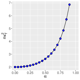
Figure 3: Role of block sizes in asymptotic variance with $B_{t}={\lceil t^{\alpha}\rceil}$ and $T=30000$.

In the following, we briefly discuss the expressions of $G$ and $\nabla l(z,\theta^{*})$ in Examples 1-3.

Example 4 (continues=linear).

Suppose the error term satisfies that $\mathbb{E}(\epsilon X)=0$. It can be verified that $\nabla l(z,\theta^{*})=-(y-x^{\top}\theta^{*})x=-\epsilon X$ and $G=\mathbb{E}(XX^{\top})$ provided the corresponding expected value exists.

Example 5 (continues=lad).

Let $f(\cdot|x)$ be the conditional density of $\epsilon$ given $X=x$, and suppose that the conditional median of $\epsilon$ given $X$ is zero. We can verify that $\nabla l(z,\theta^{*})=-X\textrm{sign}(Y-X^{\top}\theta^{*})=-X\textrm{sign}(\epsilon)$ and $G=\mathbb{E}[2f(0|X)XX^{\top}]$ under some mild regularity conditions.

Example 6 (continues=logistic).

Under some standard assumptions of logistic regression, it is not difficult to verify that

$$\nabla l(z,\theta^{*})=\frac{-yx}{1+\exp(yx^{\top}\theta^{*})},\;G=\mathbb{E}\bigg{(}\frac{\exp(X^{\top}\theta^{*})}{[1+\exp(X^{\top}\theta^{*})]^{2}}XX^{\top}\bigg{)}.$$

3.3 Bootstrap Inference

The results developed in previous sections provide theoretical justifications of the proposed estimator. However, the asymptotic covariance matrix $\Sigma$ is generally unknown in practice. Classical plug-in estimators of the covariance matrix may be inefficient or infeasible in stream data settings as it may require estimating nonparametric components (please see Example 2) and autocorrelation coefficients $r(k)$. As shown in Proposition 1, the bootstrap SGD in Fang et al., (2018) may ignore the correlation among data. To address the limitations, we proposed a mini-batch bootstrap SGD algorithm for interval estimation. Before proceeding, we first introduce the following mini-batch bootstrap SGD estimators:

$$\theta_{t}^{*k}=\Pi[\theta_{t-1}^{*k}-\gamma_{t}V_{t}\widehat{H}_{t}(W_{t}^{k},\theta_{t-1}^{*k})],\textrm{ for }k=a,b,$$ (3.2)

where $V_{t}$’s are i.i.d random variables with mean one and unit variance that are independent from $Z_{t}$’s. The bootstrap version estimator at $T$-th iteration is given by

$$\overline{\theta}_{T}^{*}=\frac{1}{2T}\sum_{t=1}^{T}(\theta_{t}^{*a}+\theta_{t}^{*b}).$$

The following theorem justifies the large sample properties of $\overline{\theta}_{T}^{*}$.

Theorem 3.

Suppose that Assumptions A1-A4 are satisfied and $\mathbb{E}(|V_{t}|^{p})<\infty$ with $p$ being the constant in Assumption A2(v). Then the following statement holds:

$$\frac{T}{\sqrt{\sum_{t=1}^{T}B_{t}^{-1}}}(\overline{\theta}_{T}^{*}-\overline{\theta}_{T})\bigg{|}\mathcal{D}_{T}\xrightarrow[\text{}]{\text{$\mathbb{L}$}}N(0,\Sigma),$$

where $\mathcal{D}_{T}=\{Z_{i},i\in I_{t}\cup J_{t},t=1,\ldots,T\}$ is the data used for the first $T$ iterations, and $\Sigma$ is the covariance matrix in Theorem 2.

Theorem 3 shows that the conditional distribution of $T(\overline{\theta}_{T}^{*}-\overline{\theta}_{T})/({\sum_{t=1}^{T}B_{t}^{-1}})^{1/2}$ given $\mathcal{D}_{T}$ is asymptotically equivalent to the distribution of $T(\overline{\theta}_{T}-\theta^{*})/({\sum_{t=1}^{T}B_{t}^{-1}})^{1/2}$. A practical implication of the above results is building confidence intervals for $g(\theta^{*})$ for some differentiable function $g\mathrel{\mathop{\mathchar 58\relax}}\Theta\to\mathbb{R}$. To be specific, we can simultaneously obtain $k$ random samples of $\overline{\theta}^{*}_{T}$, say $\overline{\theta}^{*(1)}_{T},\ldots,\overline{\theta}^{*(k)}_{T}$. A $(1-\alpha)\times 100\%$ level confidence interval of $g(\theta^{*})$ can be constructed using the quantiles of the samples $g(\overline{\theta}^{*(1)}_{T}),\ldots,g(\overline{\theta}^{*(k)}_{T})$. We formally summarize this procedure in Algorithm 1. Compared with the bootstrap SGD procedure in Fang et al., (2018), Proposition 1 and Theorem 3 together highlight the necessarity of considering the correlation among observations.

Input: Data $\{Z_{t}\}_{t=1}^{\infty}$, learning rate $\gamma_{t}$, block size $B_{t}$, bootstrap sample size $k$, number of iterations $T$, initial values $\theta_{0}^{s},\theta_{0}^{*s,(j)},\overline{\theta}_{0}=0,\overline{\theta}_{0}^{*(j)}=0$ for $j=1,\ldots,k$ and $s=a,b$, significance level $\alpha\in(0,1)$

for $t=1$ to $T$ do

       Construct indexes sets $I_{t},J_{t}$ according to the block size $B_{t}$

      Update $\theta_{t}^{s}=\Pi[\theta_{t-1}^{s}-\gamma_{t}\widehat{H}_{t}(W_{t}^{s},\theta_{t-1}^{s})]$ for $s=a,b$

      Update $\overline{\theta}_{t}=\frac{t-1}{t}\overline{\theta}_{t-1}+\frac{1}{2t}(\theta_{t}^{a}+\theta_{t}^{b})$

      for $j=1$ to $k$ do

             Generate the random weight $V_{t}^{(j)}$

            Update $\theta_{t}^{*s,(j)}=\Pi[\theta_{t-1}^{*s,(j)}-\gamma_{t}V_{t}^{(j)}\widehat{H}_{t}(W_{t}^{s},\theta_{t-1}^{*s,(j)})]$ for $s=a,b$

            Update $\overline{\theta}_{t}^{*(j)}=\frac{t-1}{t}\overline{\theta}_{t-1}^{*(j)}+\frac{1}{2t}(\theta_{t}^{*a,(j)}+\theta_{t}^{*b,(j)})$

      

Let $u_{\alpha}$ and $l_{\alpha}$ be the the $1-\alpha/2$ and $\alpha/2$ quantiles of $g(\overline{\theta}_{T}^{*(1)}),\ldots,g(\overline{\theta}_{T}^{*(k)})$.

Output: point estimator $g(\overline{\theta}_{T})$, confidence interval $(l_{\alpha},u_{\alpha})$.

Algorithm 1 Bootstrap Mini-batch SGD Algorithm

4 Monte Carlo Simulation

In this section, we provide several simulation studies to demonstrate the finite-sample performances of the proposed procedure. The following six models are considered.

1. $Y_{t}=X_{t}^{\top}\beta^{*}+\alpha^{*}+\epsilon_{t}$ with $\theta^{*}=(\beta^{*\top},\alpha)^{\top}=(0.2,-0.3,0.5,-0.25)^{\top}$. The covariates $X_{t}$’s are i.i.d. generated from a multivariate normal with mean $\mu=(-0.5,0.3,-0.4)^{\top}$ and identity covariance matrix. Given $X_{t}$, the conditional distribution $\epsilon_{t}$ is normal with mean zero and variance $(\|X_{t}\|^{2}+1)/4$. The linear regression in Example 1 is applied.

2. The same setting in Model 1 is considered, except that the LAD regression in Example 2 is applied.

3. $Y_{t}=1$ if $X_{t}^{\top}\beta^{*}+\alpha^{*}+\epsilon_{t}>0$ and $Y_{t}=-1$ if $X_{t}^{\top}\beta^{*}+\alpha^{*}+\epsilon_{t}\leq 0$. Here $\theta^{*}=(\beta^{*\top},\alpha)^{\top}=(0.2,-0.3,0.5,-0.25)^{\top}$. The covariates $X_{t}$’s follow the same data generating process in Model 1, and $\epsilon_{t}$’s are i.i.d. standard logistic random variables. The logistic regression in Example 3 is applied.

4. $Y_{t}=X_{t}^{\top}\beta^{*}+\alpha^{*}+\epsilon_{t}$ with $\theta^{*}=(\beta^{*\top},\alpha)^{\top}=(0.2,-0.3,0.5,-0.25)^{\top}$. The covariates $X_{t}$ are generated from the following vector autoregressive process (VAR):

   $$X_{t}=\begin{pmatrix}-0.5\\ 0.3\\ -0.4\end{pmatrix}+\begin{pmatrix}0.4&-0.3&0.5\\ 0.6&0.3&-0.5\\ 0.1&-0.8&-0.4\\ \end{pmatrix}X_{t-1}+\delta_{t},$$

   where $\delta_{t}$’s are i.i.d standard multivariate normal random vectors. The noise satisfies $\epsilon_{t}=\widetilde{\epsilon}_{t}+\widetilde{\epsilon}_{t+1}+\widetilde{\epsilon}_{t+2}$ with $\widetilde{\epsilon}_{t}$’s being i.i.d. standard normal. We consider the linear regression in Example 1.

5. The same setting in Model 4 is considered, except that the LAD regression in Example 2 is applied.

6. $Y_{t}=1$ if $X_{t}^{\top}\beta^{*}+\alpha^{*}+\epsilon_{t}>0$ and $Y_{t}=-1$ if $X_{t}^{\top}\beta^{*}+\alpha^{*}+\epsilon_{t}\leq 0$. Here $\theta^{*}=(\beta^{*\top},\alpha)^{\top}=(0.2,-0.3,0.5,-0.25)^{\top}$. The covariates $X_{t}$’s follow the same data generating process in Model 4. The error $\epsilon_{t}=R_{t}\widetilde{\epsilon}_{t}+(1-R_{t})\widetilde{\epsilon}_{t+1}$, where $\widetilde{\epsilon}_{t}$’s are i.i.d. standard logistic random variables, and $R_{t}$’s are i.i.d. generated from Bernoulli distribution with $p=0.5$.

We consider different sample sizes with $n=10000,20000,50000,100000$. To see the impact of batch-size, we select $B_{t}=bt^{a}$ with $a=0.2,0.3,0.5,0.7$. After several experiments, we find that $b=3$ for linear models (Models 1,2,4,5) and $b=1$ for logistic models (Models 3, 6) would give satisfactory performances. Following Fang et al., (2018) and Su and Zhu, (2018), the learning rate is set to $\gamma_{t}=(t+10)^{-2/3}$. For each setting, we make use of the bootstrap procedure in Section 3.3 with $500$ bootstrap samples and $V_{t}\sim Exp(1)$ to construct $95\%$ confidence intervals for $\beta_{1}^{*},\beta_{2}^{*},\beta_{3}^{*}$. The corresponding coverage probabilities, lengths of the intervals, and mean square errors (MSE) are recorded for $1000$ replications. The initial value to start the iteration is generated from a multivariate normal with mean zero and covariance matrix $0.1\times I$. Finally, we also consider the bootstrap SGD procedure in Fang et al., (2018) as a competitor with the same learning rate, initial value, and bootstrap setting.

The numerical results are summarized in Tables 1-6, and several interesting findings can be observed. First, for all settings and all algorithms, the MSEs decrease when the sample size is increasing. Second, for Models 1-3 with i.i.d. observations, the bootstrap SGD procedure is consistent as the coverage probabilities stay around $95\%$ regardless of the sample size. However, when the data is correlated in Models 4-6, the confidence intervals provided by the bootstrap SGD are not invalid. For example, its coverage probabilities fluctuate between $97\%$ to $100\%$ in Model 4. In particular, the coverage probabilities for the three coefficients are $99.1\%$, $98\%$, and $98.2\%$ when $n=100000$. If we look at the results in Table 4, the coverage probabilities of our proposed algorithm with $a=0.3$ are approximately at $95\%$ nominal level when $n=100000$. The corresponding lengths of the confidence intervals are $0.043,0.042,0.034$, which are uniformly shorter than those of SGD, namely, $0.050,0.050,0.047$. Similar observations can be found in Models 5 and 6. Third, the numerical results reveal that coverage probabilities heavily rely on the choice of the batch size (or the value $a$). For instance, the choice with $a=0.7$ may lead to poor performances (Tables 1-3) even when sample size is large ($n=100000$), which confirms our Assumption A4. According to Tables 1-6, the choices with $a=0.2$ or $a=0.3$ can produce confidence intervals with approximately $95\%$ coverage probabilities when $n=100000$.

Table 1: Model 1: Linear regression under i.i.d. observations

		$\beta_{1}$			$\beta_{2}$			$\beta_{3}$
a	n	CP	Length		CP	Length		CP	Length		MSE
0.2	10000	0.954	0.058		0.960	0.057		0.958	0.058		0.024
	20000	0.968	0.039		0.938	0.039		0.954	0.039		0.017
	50000	0.956	0.024		0.932	0.024		0.952	0.024		0.011
	100000	0.946	0.017		0.952	0.017		0.940	0.017		0.007
0.3	10000	0.958	0.061		0.960	0.061		0.960	0.062		0.026
	20000	0.968	0.042		0.948	0.042		0.956	0.042		0.018
	50000	0.954	0.026		0.947	0.026		0.956	0.026		0.011
	100000	0.950	0.018		0.952	0.018		0.946	0.018		0.008
0.5	10000	0.970	0.073		0.946	0.072		0.926	0.076		0.031
	20000	0.964	0.050		0.924	0.050		0.932	0.052		0.022
	50000	0.972	0.031		0.930	0.031		0.934	0.032		0.014
	100000	0.950	0.021		0.956	0.021		0.942	0.022		0.010
0.7	10000	0.962	0.085		0.934	0.088		0.858	0.093		0.041
	20000	0.968	0.061		0.908	0.062		0.888	0.065		0.029
	50000	0.972	0.039		0.912	0.039		0.908	0.042		0.018
	100000	0.952	0.027		0.950	0.027		0.892	0.028		0.013
SGD	10000	0.944	0.053		0.948	0.052		0.952	0.052		0.023
	20000	0.958	0.036		0.958	0.036		0.936	0.036		0.016
	50000	0.946	0.023		0.950	0.023		0.942	0.023		0.010
	100000	0.956	0.016		0.960	0.016		0.962	0.016		0.007

Table 2: Model 2: LAD regression under i.i.d. observations

		$\beta_{1}$			$\beta_{2}$			$\beta_{3}$
a	n	CP	Length		CP	Length		CP	Length		MSE
0.2	10000	0.966	0.068		0.970	0.068		0.942	0.069		0.030
	20000	0.980	0.046		0.968	0.046		0.958	0.046		0.020
	50000	0.968	0.029		0.948	0.029		0.952	0.029		0.013
	100000	0.966	0.020		0.958	0.020		0.944	0.020		0.009
0.3	10000	0.962	0.072		0.964	0.072		0.932	0.074		0.033
	20000	0.980	0.049		0.960	0.049		0.938	0.050		0.022
	50000	0.964	0.030		0.934	0.030		0.942	0.031		0.014
	100000	0.953	0.021		0.950	0.021		0.946	0.021		0.009
0.5	10000	0.964	0.084		0.952	0.086		0.852	0.088		0.043
	20000	0.980	0.059		0.948	0.059		0.872	0.061		0.029
	50000	0.960	0.036		0.924	0.037		0.886	0.037		0.018
	100000	0.962	0.025		0.950	0.025		0.892	0.026		0.012
0.7	10000	0.968	0.097		0.876	0.102		0.716	0.108		0.059
	20000	0.978	0.071		0.896	0.072		0.732	0.077		0.041
	50000	0.958	0.045		0.902	0.046		0.790	0.048		0.026
	100000	0.966	0.032		0.902	0.032		0.806	0.034		0.018
SGD	10000	0.974	0.061		0.958	0.061		0.970	0.062		0.026
	20000	0.960	0.042		0.974	0.042		0.950	0.042		0.018
	50000	0.948	0.026		0.954	0.026		0.948	0.026		0.011
	100000	0.970	0.018		0.962	0.018		0.956	0.018		0.008

Table 3: Model 3: Logistic regression under i.i.d. observations

		$\beta_{1}$			$\beta_{2}$			$\beta_{3}$
a	n	CP	Length		CP	Length		CP	Length		MSE
0.2	10000	0.952	0.112		0.936	0.112		0.900	0.116		0.055
	20000	0.956	0.079		0.928	0.078		0.914	0.082		0.038
	50000	0.954	0.049		0.936	0.048		0.908	0.051		0.023
	100000	0.954	0.034		0.946	0.033		0.938	0.035		0.016
0.3	10000	0.960	0.120		0.900	0.122		0.846	0.126		0.066
	20000	0.952	0.087		0.916	0.086		0.918	0.091		0.046
	50000	0.954	0.055		0.926	0.054		0.924	0.057		0.028
	100000	0.948	0.038		0.944	0.037		0.947	0.039		0.019
0.5	10000	0.954	0.139		0.838	0.145		0.620	0.150		0.098
	20000	0.944	0.105		0.826	0.107		0.690	0.113		0.071
	50000	0.942	0.072		0.876	0.072		0.716	0.076		0.045
	100000	0.932	0.052		0.840	0.051		0.780	0.054		0.032
0.7	10000	0.934	0.155		0.740	0.163		0.398	0.172		0.137
	20000	0.944	0.122		0.728	0.129		0.450	0.137		0.105
	50000	0.906	0.088		0.768	0.091		0.470	0.097		0.072
	100000	0.930	0.067		0.736	0.068		0.570	0.074		0.053
SGD	10000	0.948	0.096		0.944	0.095		0.962	0.099		0.042
	20000	0.950	0.066		0.958	0.066		0.942	0.068		0.029
	50000	0.946	0.040		0.930	0.040		0.940	0.042		0.018
	100000	0.940	0.028		0.948	0.028		0.932	0.029		0.013

Table 4: Model 4: Linear regression under mixing observations

		$\beta_{1}$			$\beta_{2}$			$\beta_{3}$
a	n	CP	Length		CP	Length		CP	Length		MSE
0.2	10000	0.982	0.154		0.988	0.160		0.992	0.132		0.049
	20000	0.984	0.100		0.976	0.101		0.990	0.083		0.033
	50000	0.960	0.059		0.974	0.057		0.974	0.045		0.021
	100000	0.958	0.040		0.962	0.037		0.956	0.030		0.014
0.3	10000	0.986	0.168		0.990	0.179		0.992	0.148		0.050
	20000	0.990	0.111		0.982	0.117		0.990	0.097		0.035
	50000	0.958	0.064		0.962	0.064		0.960	0.052		0.022
	100000	0.953	0.043		0.954	0.042		0.950	0.034		0.015
0.5	10000	0.990	0.201		0.994	0.229		0.996	0.189		0.056
	20000	0.992	0.139		0.994	0.156		0.994	0.129		0.040
	50000	0.970	0.079		0.990	0.086		0.988	0.070		0.025
	100000	0.978	0.054		0.986	0.057		0.994	0.046		0.017
0.7	10000	0.986	0.234		0.998	0.276		0.996	0.226		0.063
	20000	0.992	0.166		0.994	0.195		0.998	0.158		0.046
	50000	0.982	0.099		0.996	0.113		0.992	0.092		0.030
	100000	0.980	0.068		0.996	0.077		0.990	0.062		0.020
SGD	10000	0.996	0.135		0.992	0.132		0.998	0.132		0.042
	20000	0.986	0.104		0.976	0.103		0.996	0.101		0.031
	50000	0.988	0.073		0.976	0.072		0.992	0.070		0.020
	100000	0.991	0.050		0.980	0.050		0.982	0.047		0.014

Table 5: Model 5: LAD regression under mixing observations

		$\beta_{1}$			$\beta_{2}$			$\beta_{3}$
a	n	CP	Length		CP	Length		CP	Length		MSE
0.2	10000	0.966	0.162		0.956	0.143		0.976	0.118		0.061
	20000	0.962	0.109		0.964	0.103		0.978	0.082		0.043
	50000	0.954	0.067		0.958	0.066		0.957	0.052		0.027
	100000	0.954	0.047		0.960	0.046		0.956	0.036		0.018
0.3	10000	0.978	0.171		0.960	0.148		0.970	0.125		0.064
	20000	0.964	0.118		0.964	0.109		0.972	0.089		0.045
	50000	0.956	0.072		0.958	0.071		0.960	0.056		0.029
	100000	0.952	0.050		0.957	0.050		0.951	0.039		0.020
0.5	10000	0.938	0.199		0.968	0.164		0.940	0.143		0.076
	20000	0.956	0.141		0.964	0.122		0.964	0.103		0.054
	50000	0.942	0.088		0.976	0.085		0.958	0.067		0.035
	100000	0.954	0.060		0.962	0.062		0.960	0.049		0.024
0.7	10000	0.896	0.230		0.964	0.183		0.908	0.166		0.094
	20000	0.908	0.169		0.964	0.138		0.918	0.121		0.068
	50000	0.916	0.110		0.970	0.097		0.926	0.081		0.044
	100000	0.930	0.076		0.962	0.074		0.930	0.060		0.031
SGD	10000	0.898	0.119		0.918	0.112		0.970	0.106		0.054
	20000	0.902	0.083		0.912	0.076		0.970	0.073		0.037
	50000	0.892	0.051		0.900	0.046		0.964	0.045		0.024
	100000	0.904	0.036		0.910	0.032		0.950	0.031		0.017

Table 6: Model 6: Logistic regression under mixing observations

		$\beta_{1}$			$\beta_{2}$			$\beta_{3}$
a	n	CP	Length		CP	Length		CP	Length		MSE
0.2	10000	0.954	0.079		0.928	0.077		0.904	0.078		0.033
	20000	0.950	0.054		0.908	0.054		0.912	0.053		0.023
	50000	0.954	0.033		0.934	0.033		0.932	0.032		0.014
	100000	0.948	0.022		0.945	0.022		0.944	0.022		0.009
0.3	10000	0.950	0.087		0.936	0.085		0.934	0.087		0.035
	20000	0.958	0.059		0.912	0.060		0.938	0.060		0.025
	50000	0.962	0.036		0.932	0.037		0.936	0.036		0.015
	100000	0.954	0.024		0.946	0.026		0.945	0.025		0.010
0.5	10000	0.924	0.112		0.954	0.104		0.974	0.114		0.044
	20000	0.954	0.077		0.926	0.077		0.964	0.080		0.031
	50000	0.950	0.047		0.938	0.050		0.978	0.049		0.019
	100000	0.962	0.032		0.930	0.036		0.960	0.034		0.014
0.7	10000	0.826	0.138		0.976	0.124		0.950	0.145		0.061
	20000	0.888	0.100		0.942	0.095		0.960	0.107		0.043
	50000	0.908	0.064		0.942	0.064		0.960	0.068		0.027
	100000	0.904	0.044		0.944	0.048		0.962	0.049		0.020
SGD	10000	0.922	0.064		0.910	0.062		0.870	0.064		0.030
	20000	0.914	0.044		0.894	0.042		0.896	0.044		0.020
	50000	0.918	0.027		0.924	0.026		0.892	0.027		0.012
	100000	0.916	0.019		0.916	0.018		0.902	0.019		0.009

5 Empirical Application

In this section, we apply the proposed procedure to the POWER dataset from UCI Machine Learning Repository (Dua and Graff,, 2017). The POWER dataset contains $2075259$ measurements of electric power consumption gathered in a house located in Sceaux during $47$ months. After removing missing values, we keep a record of $2049280$ observations. We divide the time of a day into three periods: (a) morning from 0:00 to 12:00; (b) afternoon from 12:00 to 18:00; (c) evening from 18:00 to 24:00. We apply the linear regression and the LAD regression based on the following four models:

1. $\textrm{Power}=\beta_{11}\textrm{morning}+\beta_{12}\textrm{afternoon}+\beta_{13}\textrm{evening}+\textrm{error}$;

2. $\textrm{Sub-Metering 1}=\beta_{21}\textrm{morning}+\beta_{22}\textrm{afternoon}+\beta_{23}\textrm{evening}+\textrm{error}$;

3. $\textrm{Sub-Metering 2}=\beta_{31}\textrm{morning}+\beta_{32}\textrm{afternoon}+\beta_{33}\textrm{evening}+\textrm{error}$;

4. $\textrm{Sub-Metering 3}=\beta_{41}\textrm{morning}+\beta_{42}\textrm{afternoon}+\beta_{42}\textrm{evening}+\textrm{error}.$

Here Power is the household global minute-averaged active power (in kilowatt), Sub-metering 1 corresponds to the active energy used by kitchen, Sub-metering 2 is the energy consumption in the laundry room, Sub-Metering 3 records the energy consumed by electric water-heaters and air-conditioners, and the covariates are the corresponding dummies. The observations of Sub-metering 1-3 are recorded in watt-hour. The batch size is set to $\gamma_{t}=3t^{a}$ with $a=0.3$, while the choice of the initial values and the bootstrap setting follow those in the simulation studies. The point estimates and the corresponding $95\%$ confidence intervals are provided in Tables 7 and 8. The results suggest that the error terms are right-skewed as the linear regression gives larger coefficients than the LAD regression. Moreover, both Tables 7 and 8 reveals that the electronic power consumption in the afternoon and evening is higher than that in the morning. If we look at Models 2 and 3, the corresponding estimates in Table 8 are almost zero, which are significantly smaller than the estimates in Table 7. This is due to the fact that $91.7\%$ and $70\%$ observations of Sub-Metering 1 and Sub-Metering 2 are zeros, while Sub-Metering 3 contains $41.4\%$ zeros. Finally, we plot the histograms of $k=500$ bootstrap samples for each coefficient estimates, which are summarized in Figures 4 and 5. The plots suggests that the bootstrap procedure can be used to approximate the sample distribution of the proposed estimator even if the distribution is skewed. For example, the last histogram in Fig 5 is relatively skewed, and the proposed bootstrap procedure is able to capture such skewness.

Table 7: Estimation of linear regression models.

	Model 1			Model 2			Model 3			Model 4
	Est.	$95\%$ CI		Est.	$95\%$ CI		Est.	$95\%$ CI		Est.	$95\%$ CI
Morning	0.9131	(0.8986, 0.9255)		0.5905	(0.5468, 0.6368)		0.7781	(0.7309, 0.8316)		6.0587	(5.9231, 6.1794)
Afternoon	1.1153	(1.0922, 1.1420)		1.2777	(1.1676, 1.3743)		2.2729	(2.1225, 2.4284)		6.9532	(6.7618, 7.1491)
Evening	1.6188	(1.5879, 1.6427)		2.1710	(2.0502, 2.2880)		1.8240	(1.6955, 1.9507)		6.5019	(6.3222, 6.6638)

Table 8: Estimation of LAD regression models.

	Model 1			Model 2			Model 3			Model 4
	Est.	$95\%$ CI		Est.	$95\%$ CI		Est.	$95\%$ CI		Est.	$95\%$ CI
Morning	0.4931	(0.4676, 0.5111)		0.0005	(0.0003, 0.0013)		0.0025	(0.0031, 0.0053)		0.5012	(0.4925, 0.5164)
Afternoon	0.7354	(0.7091, 0.7695)		0.0006	(-0.0009, 0.0024)		0.0036	(0.0041, 0.0086)		0.9057	(0.6816, 1.4741)
Evening	1.4209	(1.3715, 1.4554)		0.0009	(0.0006, 0.0018)		0.0055	(0.0059, 0.0152)		0.7594	(0.4737, 1.4865)

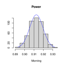
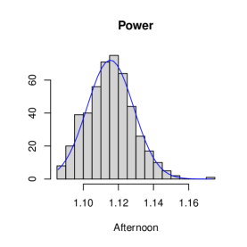
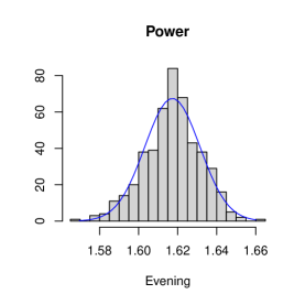
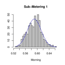
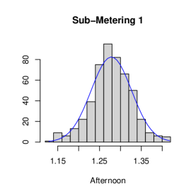
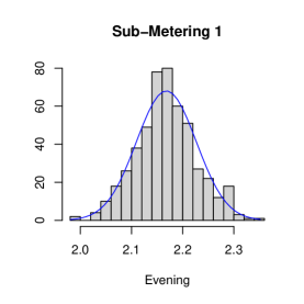
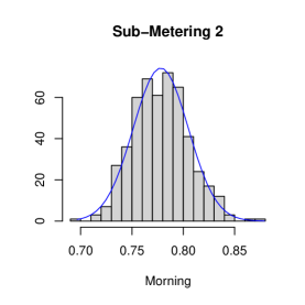
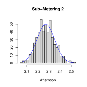
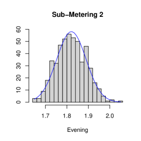
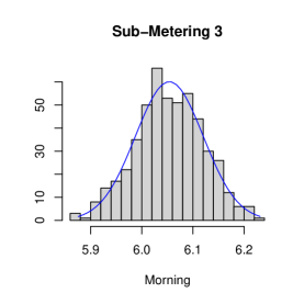
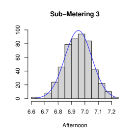
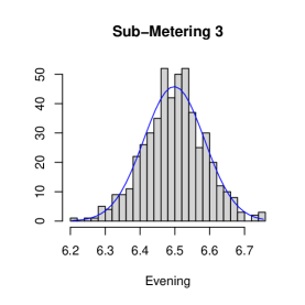
Figure 4: Bootstrap histograms of linear regression models.

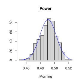
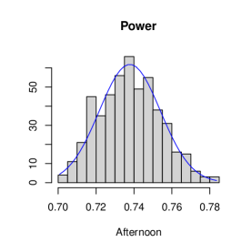
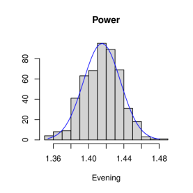
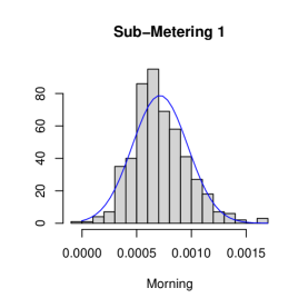
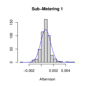
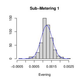
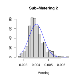
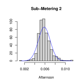
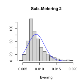
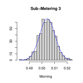
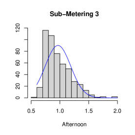
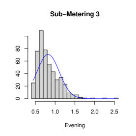
Figure 5: Bootstrap histograms of LAD regression models.

6 Conclusion

In this paper, we proposed a mini-batch SGD algorithm to conduct statistical inference about the system parameters when the observations are $\phi$-mixing. The proposed algorithm is applicable to both smooth and non-smooth loss functions, which can cover many popular statistical models. In addition, a mini-batch bootstrap SGD procedure is developed to construct confidence intervals. The limiting distribution of the mini-batch SGD estimator and the validity of the bootstrap procedure are both established. To demonstrate the risk of ignoring the correlation, we also design a concrete example showing the invalidity of the bootstrap SGD in Fang et al., (2018) when the observations are correlated. Monte Carlo simulations and an application to a real-world dataset are conducted to examine the finite sample properties of the proposed method, and the results confirm our theoretical findings.

Supplement

Supplement to “Statistical Inference with Stochastic Gradient Methods under $\phi$-mixing Data”

This supplement includes the proofs of the main theorems. Section S.I provides the proofs of some technical lemmas. The proofs of Theorems 1-3 are given in Sections S.II-S.IV, respectively. We prove Proposition 1 in Section S.V, and additional numerical results are included in Section S.VI.

Since $\theta_{T}^{a}$ (or $\theta_{T}^{*a}$) plays a similar role as $\theta_{T}^{b}$ (or $\theta_{T}^{*b}$), it suffices to study the former. For ease of presentation, we drop the superscript in (2.1) and (3.2). Moreover, iteration procedures in (2.1) and (3.2) can be generalized as follows:

$$\theta_{t}=\Pi[\theta_{t-1}-\gamma_{t}U_{t}\widehat{H}_{t}(W_{t},\theta_{t-1})].$$ (S.1)

where $U_{t}$’s are i.i.d random variables satisfying Assumption B1, and $W_{t}=W_{t}^{a}$ after dropping the superscript.

Assumption B1.

The i.i.d. random variables $U_{j}$’s are independent from the observations $Z_{j}$’s. Moreover, it holds that $\mathbb{E}(U_{j})=1$ and $\mathbb{E}(|U_{j}|^{p})<\infty$. Here $p$ is the constant introduced in Assumption A2(v).

Clearly, $\theta_{t}$ becomes the estimators in (2.1) when $U_{t}=1$, and it is identical to bootstrap estimators in (3.2) when $U_{t}=V_{t}$. Before proceeding, let us define an ancillary time series $\widetilde{\mathbf{Z}}=\{\widetilde{Z}_{t}\}_{t=1}^{\infty}$, which has the same distribution as $\mathbf{Z}=\{Z_{t}\}_{t=1}^{\infty}$ and is independent from $\mathbf{Z}$ and $U_{t}$’s. Similarly, we define $\widetilde{W}_{t}=\{\widetilde{Z}_{i},i\in I_{t}\}$, which is identically distributed as $W_{t}$. Moreover, we will use the following notation:

$$\mathbb{E}_{t-1}(\cdot) = \mathbb{E}(\cdot|W_{1},\ldots,W_{t-1}),$$

$$H(\theta) = \mathbb{E}[\nabla l(Z,\theta)]=\nabla L(\theta),$$

$$e_{t} = \mathbb{E}_{t-1}[\widehat{H}_{t}(W_{t},\theta_{t-1})]-H(\theta_{t-1}),$$

$$\zeta_{t} = U_{t}\widehat{H}_{t}({W}_{t},\theta_{t-1})-\mathbb{E}_{t-1}[\widehat{H}_{t}(W_{t},\theta_{t-1})],$$

$$\widetilde{\zeta}_{t} = U_{t}\widehat{H}_{t}(\widetilde{W}_{t},\theta_{t-1})-\mathbb{E}_{t-1}[\widehat{H}_{t}(\widetilde{W}_{t},\theta_{t-1})]=U_{t}\widehat{H}_{t}(\widetilde{W}_{t},\theta_{t-1})-H(\theta_{t-1}).$$

Hence, the iteration in (S.1) can be written as

$$\theta_{t}=\Pi[\theta_{t-1}-\gamma_{t}H(\theta_{t-1})-\gamma_{t}e_{t}-\gamma_{t}\zeta_{t}].$$

S.I Preliminary Lemmas

Lemma S.1.

Let $X_{1},X_{2},\ldots$ be a stationary sequence with the $\phi$-mixing coefficients bounded by $\phi(t)$. Moreover, assume that $\sum_{t=1}^{\infty}\phi^{1/2}(t)<\infty$, $\mathbb{E}(X_{t})=0$, and $\mathbb{E}(\|X_{t}\|^{k})<\infty$ for some constant $k>2$. Then it follows that $\mathbb{E}(|\sum_{t=1}^{T}X_{t}|^{k})\leq C_{k}T^{k/2}$, where $C_{k}$ is some constant relying on $k$.

Proof.

It follows from Theorem 3 in Yokoyama, (1980). ∎

Lemma S.2.

Let $X$ be a real random variable on a probability space $(\Omega,\mathcal{A},P)$ with $\|X\|_{\infty}<\infty$. Then

$$\sup_{A\in\mathcal{A},P(A)>0}\frac{1}{P(A)}\left|\int_{A}XdP\right|=\|X\|_{\infty}.$$

Proof.

If $M\geq 0$ is a constant such that $\|X\|_{\infty}\leq M$, and $A\in\mathcal{A}$ is such that $P(A)>0$, then it follows that $P^{-1}(A)|\int_{A}XdP|\leq M$, which further implies that $P^{-1}(A)|\int_{A}XdP|\leq\|X\|_{\infty}$.

Now for any $\epsilon>0$ small enough such that $\|X\|_{\infty}-\epsilon>0$, let us define

$$F^{+} = \{X\geq\|X\|_{\infty}-\epsilon\},$$

$$F^{-} = \{-X\geq\|X\|_{\infty}-\epsilon\},$$

$$F = \begin{cases}F^{+}&\textrm{ if }P(F^{+})\geq P(F^{-});\\ F^{-}&\textrm{ otherwise}.\end{cases}$$

Then we show that $P^{-1}(F)|\int_{F}XdP|\geq\|X\|_{\infty}-\epsilon$. Since $\epsilon>0$ is arbitrary, we complete the proof. ∎

Lemma S.3.

Consider the probability space $(\Omega,\mathcal{A}\bigotimes\mathcal{B},Q)$. It follows that $\sum_{i=1}^{k}|Q(B_{i}|\mathcal{A})-Q_{2}(B_{i})|\leq 2\phi_{Q}(\mathcal{B},\mathcal{A})$ for any integer $k$ and any sets $B_{1},\ldots,B_{k}\in\mathcal{B}$.

Proof.

First let us prove

$$|Q(B|\mathcal{A})-Q(B)|\leq\phi_{Q}(\mathcal{B},\mathcal{A}).$$ (S.2)

Let $X=Q(B|\mathcal{A})-Q(B)$, and direct examination leads to

$$\frac{1}{Q(A)}\left|\int_{A}XdQ\right|=\frac{1}{Q(A)}\left|Q(B\cap A)-Q(B)Q(A)\right|=\left|Q(B|A)-Q(B)\right|.$$

By Lemma S.2 and the above equation, we have

$$\left|Q(B|\mathcal{A})-Q(B)\right|=|X|\leq\|X\|_{\infty}=\sup_{A\in\mathcal{A},Q(A)>0}\left|Q(B|A)-Q(B)\right|\leq\phi_{Q}(\mathcal{B},\mathcal{A}),$$

which proves (S.2). Let us define

$$I_{+}=\{i\mathrel{\mathop{\mathchar 58\relax}}Q(B_{i}|\mathcal{A})-Q(B_{i})\geq 0\}\textrm{ and }I_{-}=\{i\mathrel{\mathop{\mathchar 58\relax}}Q(B_{i}|\mathcal{A})-Q(B_{i})<0\}.$$

As a consequence, we have

$$\sum_{i=1}^{k}|Q(B_{i}|\mathcal{A})-Q(B_{i})| = \sum_{i\in I_{+}}[Q(B_{i}|\mathcal{A})-Q(B_{i})]-\sum_{i\in I_{-}}[Q(B_{i}|\mathcal{A})-Q(B_{i})]$$

$$= [Q(\cup_{i\in I_{+}}B_{i}|\mathcal{A})-Q(\cup_{i\in I_{+}}B_{i})]-[Q(\cup_{i\in I_{-}}B_{i}|\mathcal{A})-Q(\cup_{i\in I_{-}}B_{i})]$$

$$\leq 2\phi_{Q}(\mathcal{B},\mathcal{A}),$$

where the last inequality follows from (S.2). ∎

Lemma S.4.

Consider the probability space $(\Omega,\mathcal{A}\bigotimes\mathcal{B},Q)$, and the marginal probability of $Q$ is $Q_{1}$ and $Q_{2}$. Let $P=Q_{1}\times Q_{2}$ be the product measure. For any measurable function $h\in\mathcal{A}\bigotimes\mathcal{B}$, it follows that

$$|Q(h|\mathcal{A})-P(h|\mathcal{A})|^{p}\leq C_{p}[Q(|h|^{p})+P(|h|^{p})]\phi_{Q}^{p-1}(\mathcal{B},\mathcal{A}),$$

where $C_{p}>0$ is a constant relying on $p$. In particular, if $|h|\leq K$, it holds that

$$|Q(h|\mathcal{A})(x)-P(h|\mathcal{A})(x)|\leq K\phi_{Q}(\mathcal{B},\mathcal{A}).$$

Proof.

For simplicity, let $q=(1-1/p)^{-1}$. First, let us assume $h=\sum_{i=1}^{k}a_{i}I_{D_{i}}(x,y)$ is a simple function, where $D_{1},\ldots,D_{k}\in\mathcal{A}\bigotimes\mathcal{B}$ are disjoint and $a_{1},\ldots,a_{k}\in\mathbb{R}$. By simple algebra, it follows that

$$Q(I_{D_{i}}|\mathcal{A})(x)=\int I_{D_{i}}(x,y)Q(x,dy)=\int I_{D_{i}^{x}}(y)Q(x,dy)=Q(D_{i}^{x}|\mathcal{A})(x).$$

Here $D_{i}^{x}=\{y\mathrel{\mathop{\mathchar 58\relax}}(x,y)\in D_{i}\}$. Similarly, we have $P(I_{D_{i}}|\mathcal{A})(x)=P(D_{i}^{x}|\mathcal{A})(x)=Q_{2}(D_{i}^{x})(x).$ For any $x\in\Omega_{\mathcal{A}}$, it follows that

$$|Q(h|\mathcal{A})(x)-P(h|\mathcal{A})(x)|^{p}$$

$$= \left|\sum_{i=1}^{k}a_{i}\left[\int I_{D_{i}^{x}}(y)Q(x,dy)-\int I_{D_{i}^{x}}(y)Q_{2}(dy)\right]\right|^{p}$$

$$= \left|\sum_{i=1}^{k}a_{i}\left[Q(D_{i}^{x}|\mathcal{A})(x)-Q_{2}(D_{i}^{x})(x)\right]\right|^{p}$$

$$\leq \left[\sum_{i=1}^{k}|a_{i}|\left|Q(D_{i}^{x}|\mathcal{A})(x)-Q_{2}(D_{i}^{x})(x)\right|\right]^{p}$$

$$\leq \left[\sum_{i=1}^{k}|a_{i}|\left|Q(D_{i}^{x}|\mathcal{A})(x)-Q_{2}(D_{i}^{x})(x)\right|^{1/p}\left|Q(D_{i}^{x}|\mathcal{A})(x)-Q_{2}(D_{i}^{x})(x)\right|^{1/q}\right]^{p}$$

$$\leq \left[\sum_{i=1}^{k}|a_{i}|^{p}\left|Q(D_{i}^{x}|\mathcal{A})(x)-Q_{2}(D_{i}^{x})(x)\right|\right]\left[\sum_{i=1}^{k}\left|Q(D_{i}^{x}|\mathcal{A})(x)-Q_{2}(D_{i}^{x})(x)\right|\right]^{p/q}$$

$$\leq [Q(|h|^{p}|\mathcal{A})(x)+P(|h|^{p}|\mathcal{A})(x)]\left[\sum_{i=1}^{k}\left|Q(D_{i}^{x}|\mathcal{A})(x)-Q_{2}(D_{i}^{x})(x)\right|\right]^{p/q}.$$

Using Lemma S.3, we show that

$$|Q(h|\mathcal{A})(x)-P(h|\mathcal{A})(x)|^{p}\leq 2^{p/q}[Q(|h|^{p}|\mathcal{A})+P(|h|^{p}|\mathcal{A})]\phi_{Q}^{p/q}(\mathcal{B},\mathcal{A}).$$ (S.3)

Similarly, when $|a_{i}|\leq K$, we have

$$|Q(h|\mathcal{A})(x)-P(h|\mathcal{A})(x)| = \left|\sum_{i=1}^{k}a_{i}\left[\int I_{D_{i}^{x}}(y)Q(x,dy)-\int I_{D_{i}^{x}}(y)Q_{2}(dy)\right]\right|$$

$$= \left|\sum_{i=1}^{k}a_{i}\left[Q(D_{i}^{x}|\mathcal{A})(x)-Q_{2}(D_{i}^{x})(x)\right]\right|$$

$$\leq \max_{1\leq i\leq k}|a_{i}|\sum_{i=1}^{k}\left|Q(D_{i}^{x}|\mathcal{A})(x)-Q_{2}(D_{i}^{x})(x)\right|.$$

Lemma S.3 implies that

$$|Q(h|\mathcal{A})(x)-P(h|\mathcal{A})(x)|\leq K\phi_{Q}(\mathcal{B},\mathcal{A}).$$ (S.4)

For a general measure function $h$, there exists a sequence of simple functions $h_{n}$ such that $h_{n}\to h$ pointwise and $h_{n}\leq h$. Using monotone convergence theorem, we show that the (S.3) holds for $h$. In addition, if $|h|\leq K$, we can apply similar argument to show that (S.4) holds for $h$. ∎

Lemma S.5.

Let $(X,Y)$ and $(X,\widetilde{Y})$ be random vectors such that $X$ and $\widetilde{Y}$ are independent. Moreover, let $Y$ and $\widetilde{Y}$ have the same marginal distribution. Then it follows that

$$\|\mathbb{E}[h(X,Y)|X]-\mathbb{E}[h(X,\widetilde{Y})|X]\|\leq m\phi(X,Y)+\frac{\mathbb{E}(\|h(X,Y)\|^{p}|X)}{m^{p-1}}+\frac{\mathbb{E}(\|h(X,\widetilde{Y})\|^{p}|X)}{m^{p-1}},$$

where $m>0$ is an arbitrary constant. Moreover, it holds that

$$\|\mathbb{E}[h(X,Y)|X]-\mathbb{E}[h(X,\widetilde{Y})|X]\|^{p}\leq C_{p}\left(\mathbb{E}[\|h(X,Y)\|^{p}|X]+\mathbb{E}[\|h(X,\widetilde{Y})\|^{p}|X]\right)\phi^{p-1}(X,Y),$$

where $C_{p}>0$ is a constant relying on $p$.

Proof.

For simplicity, let us assume $h(x,y)$ is a scalar, as it is easy to extend to the vector case. Let $h_{1}(x,y)=h(x,y)I(|h(x,y)|\leq m)$ and $h_{2}(x,y)=h(x,y)I(|h(x,y)|>m)$. Using Lemma S.4, we have

$$|\mathbb{E}[h_{1}(X,Y)|X]-\mathbb{E}[h_{1}(X,\widetilde{Y})|X]|\leq m\phi(X,Y).$$

Moreover, it follows that

$$\mathbb{E}(|h_{2}(X,Y)||X)\leq\frac{\mathbb{E}(|h(X,Y)|^{p}|X)}{m^{p-1}}\;\textrm{ and }\;\mathbb{E}(|h_{2}(X,\widetilde{Y})||X)\leq\frac{\mathbb{E}(|h(X,\widetilde{Y})|^{p}|X)}{m^{p-1}}.$$

Combining the above inequalities, we complete the proof of the first statement. The second statement follows from Lemma S.4. ∎

Lemma S.6.

Suppose that $a_{n}>0$ is a decreasing sequence with $\lim_{n\to\infty}a_{n}=0$, and $b_{n}$ is a converging sequence with $\lim_{n\to\infty}b_{n}=b$. If $\sum_{n=1}^{\infty}a_{n}=\infty$, then $\lim_{T\to\infty}{\sum_{n=1}^{T}a_{n}b_{n}}/{\sum_{n=1}^{T}a_{n}}=b$.

Proof.

For any $\epsilon>0$, there exists a constant $N>0$ such that $|b_{n}-b|<\epsilon$ for all $n\geq N$. As a consequence, it follows that

$$\bigg{|}\frac{\sum_{n=1}^{T}a_{n}b_{n}}{\sum_{n=1}^{T}a_{n}}-b\bigg{|} = \bigg{|}\frac{\sum_{n=1}^{T}a_{n}(b_{n}-b)}{\sum_{n=1}^{T}a_{n}}\bigg{|}$$

$$\leq \bigg{|}\frac{\sum_{n=1}^{N}a_{n}(b_{n}-b)}{\sum_{n=1}^{T}a_{n}}\bigg{|}+\bigg{|}\frac{\sum_{n=N+1}^{T}a_{n}(b_{n}-b)}{\sum_{n=1}^{T}a_{n}}\bigg{|}$$

$$\leq \bigg{|}\frac{\sum_{n=1}^{N}a_{n}(b_{n}-b)}{\sum_{n=1}^{T}a_{n}}\bigg{|}+\epsilon.$$

Let $T\to\infty$, since $\sum_{n=1}^{\infty}a_{n}=\infty$, we conclude that $\lim_{T\to\infty}\left|{\sum_{n=1}^{T}a_{n}b_{n}}/{\sum_{n=1}^{T}a_{n}}-b\right|\leq\epsilon.$ Notice that $\epsilon>0$ is arbitrary, we complete the proof. ∎

Lemma S.7.

Suppose that $a_{n}>0$ is a decreasing sequence with $\lim_{n\to\infty}a_{n}=0$, and $b_{n}$ is a sequence with $\sum_{n=1}^{\infty}|b_{n}|<\infty$. If $\sum_{n=1}^{\infty}a_{n}=\infty$, then $\lim_{T\to\infty}{\sum_{n=1}^{T}a_{n}\sum_{k=n}^{T}b_{k}}/{\sum_{n=1}^{T}a_{n}}=0$.

Proof.

Notice that $|\sum_{k=n}^{T}b_{k}|\leq\sum_{k=n}^{\infty}|b_{k}|\to 0$ as $n\to\infty$. Applying Lemma S.6, we get the desired results. ∎

Lemma S.8.

Let $a(x)$ be a function on $\mathbb{R}$, and let $k<n$ be two integers.

1. If $a(x)$ is non-decreasing, then $\int_{k-1}^{n}a(x)dx\leq\sum_{i=k}^{n}a(i)\leq\int_{k}^{n+1}a(x)dx$.

2. If $a(x)$ is non-increasing, then $\int_{k}^{n+1}a(x)dx\leq\sum_{i=k}^{n}a(i)\leq\int_{k-1}^{n}a(x)dx$.

Proof.

Suppose that $a(x)$ is non-decreasing. It follows that

$$\sum_{i=k}^{n}a(i)=\sum_{i=k}^{n}\int_{i}^{i+1}a(i)dx\leq\sum_{i=k}^{n}\int_{i}^{i+1}a(x)dx=\int_{k}^{n+1}a(x)dx$$

and

$$\sum_{i=k}^{n}a(i)=\sum_{i=k}^{n}\int_{i-1}^{i}a(i)dx\geq\sum_{i=k}^{n}\int_{i-1}^{i}a(x)dx=\int_{k-1}^{n}a(x)dx.$$

Similarly, if $a(x)$ is non-increasing, we have

$$\sum_{i=k}^{n}a(i)=\sum_{i=k}^{n}\int_{i}^{i+1}a(i)dx\geq\sum_{i=k}^{n}\int_{i}^{i+1}a(x)dx=\int_{k}^{n+1}a(x)dx$$

and

$$\sum_{i=k}^{n}a(i)=\sum_{i=k}^{n}\int_{i-1}^{i}a(i)dx\leq\sum_{i=k}^{n}\int_{i-1}^{i}a(x)dx=\int_{k-1}^{n}a(x)dx.$$

∎

Lemma S.9.

Let $a_{j}=e^{Kj^{\alpha}}$ for some $\alpha\in(0,1)$ and $K>0$, then $\sup_{j\geq 1}a_{j+1}/a_{j}<\infty$.

Proof.

By direct examination, it follows that

$$\log\bigg{(}\frac{a_{j+1}}{a_{j}}\bigg{)}=K(j+1)^{\alpha}-Kj^{\alpha}=Kj^{\alpha}[(1+1/j)^{\alpha}-1].$$

Since $(1+x)^{\alpha}\leq 1+\alpha x$ for all $x\geq 0$ when $\alpha\in(0,1)$, we have

$$\log\bigg{(}\frac{a_{j+1}}{a_{j}}\bigg{)}\leq Kj^{\alpha}\frac{\alpha}{j}=\alpha Kj^{-1+\alpha}\leq\alpha K,$$

which further implies the desired result. ∎

Lemma S.10.

Let $G$ be a positive definite matrix and define

$$D_{j}^{j} = I,$$

$$D_{j}^{t} = (I-\gamma_{t-1}G)D_{j}^{t-1}=\ldots=\prod_{k=j}^{t-1}(I-\gamma_{k}G)\;\textrm{ for }t\geq j,$$

$$\overline{D}_{j}^{t} = \gamma_{j}\sum_{i=j}^{t-1}D_{j}^{i}=\gamma_{j}\sum_{i=j}^{t-1}\prod_{k=j}^{i-1}(I-\gamma_{k}G).$$

and the sequence $\{\gamma_{t}\}_{t=1}^{\infty}$ satisfies $\gamma_{t}=(t+\gamma)^{-\rho}$ for some $\gamma>0$ and $\rho\in(1/2,1)$. Then the following statements hold:

1. There are constants $C>0$ such that $\|\overline{D}_{j}^{t}\|\leq C\textrm{ for all }j\textrm{ and all }t\geq j$.

2. $\lim_{t\to\infty}\frac{1}{t}\sum_{j=1}^{t}\|\overline{D}_{j}^{t}-G^{-1}\|=0$.

3. $\|D_{j}^{t}\|\leq\exp(-\lambda_{G}\sum_{k=j}^{t-1}(k+\gamma)^{-\rho})$, where $\lambda_{G}$ is the smallest eigenvalue of $G$.

4. Suppose that $\{a_{j}\}_{j=0}^{\infty}$ is a positive and non-increasing sequence such that $\sum_{j=0}^{\infty}a_{j}=\infty$ and $t^{\rho}/(\sum_{j=1}^{t}a_{j})\to 0$, then $\lim_{t\to\infty}\sum_{j=1}^{t}a_{j}\|\overline{D}_{j}^{t}-G^{-1}\|/\sum_{j=1}^{t}a_{j}=0.$

Proof.

The statements (i) and (ii) are the conclusions of Lemma 1 in Polyak and Juditsky, (1992), while statement (iii) is Lemma D.2 from Chen et al., (2020). We will prove (iv) in the following. Since $D_{j}^{i+1}=(I-\gamma_{i}G)D_{j}^{i}=D_{j}^{i}-\gamma_{i}GD_{j}^{i}$, taking summation implies that

$$D_{j}^{t}=D_{j}^{j}-\sum_{i=j}^{t-1}\gamma_{i}GD_{j}^{i}=I-G\sum_{i=j}^{t-1}\gamma_{i}D_{j}^{i}.$$

Direct examination leads to

$$\sum_{i=j}^{t-1}\gamma_{i}D_{j}^{i}=\gamma_{j}\sum_{i=j}^{t-1}D_{j}^{i}+\gamma_{j}\sum_{i=j}^{t-1}(\gamma_{i}-\gamma_{j})D_{j}^{i}\mathrel{\mathop{\mathchar 58\relax}}=\overline{D}_{j}^{t}+S_{j}^{t},$$

which further implies that

$$G^{-1}D_{j}^{t}+S_{j}^{t}=G^{-1}-\overline{D}_{j}^{t}.$$ (S.5)

Using statement (iii), we see that

$$\|S_{j}^{t}\|\leq\gamma_{j}\sum_{i=j}^{t-1}(\gamma_{j}-\gamma_{i})\|D_{j}^{i}\|\leq\gamma^{2}j^{-2\rho}\sum_{i=j}^{t-1}\exp\bigg{(}-\gamma\lambda_{G}\sum_{k=j}^{i-1}k^{-\rho}\bigg{)}\leq\gamma^{2}j^{-2\rho}\sum_{i=j}^{\infty}\exp\bigg{(}-\gamma\lambda_{G}\sum_{k=j}^{i-1}k^{-\rho}\bigg{)}.$$

Since $\sum_{k=j}^{i-1}k^{-\rho}\geq\int_{j}^{i}x^{-\rho}dx=(1-\rho)^{-1}(i^{1-\rho}-j^{1-\rho})$, the above inequality further implies that

$$\|S_{j}^{t}\| \leq \gamma^{2}j^{-2\rho}\sum_{i=j}^{\infty}\exp\bigg{(}-\gamma\lambda_{G}(1-\rho)^{-1}(i^{1-\rho}-j^{1-\rho})\bigg{)}$$

$$= \gamma^{2}j^{-2\rho}\frac{\sum_{i=j}^{\infty}e^{-\gamma\lambda_{G}(1-\rho)^{-1}i^{1-\rho}}}{e^{-\gamma\lambda_{G}(1-\rho)^{-1}j^{1-\rho}}}\leq\gamma^{2}j^{-2\rho}\frac{\sum_{i=j}^{\infty}g(i)}{g(j)},$$

where $g(x)=e^{-\gamma\lambda_{G}(1-\rho)^{-1}x^{1-\rho}}$. Since $g(x)$ is decreasing, it follows that

$$\|S_{j}^{t}\|\leq\gamma^{2}\frac{\int_{j}^{\infty}g(x)dx+g(j)}{j^{2\rho}g(j)}.$$

Notice that $\int_{j}^{\infty}g(x)dx\to 0$ and $j^{\rho}g(j)\to 0$ as $j\to\infty$, using L’Hospital’s rule, we obtain that

$$\lim_{j\to\infty}\frac{\int_{j}^{\infty}g(x)dx}{j^{2\rho}g(j)} = \lim_{j\to\infty}\frac{-g(j)}{j^{2\rho}g^{\prime}(j)+2\rho j^{2\rho-1}g(j)}$$

$$= \lim_{j\to\infty}\frac{-e^{-\gamma\lambda_{G}(1-\rho)^{-1}j^{1-\rho}}}{[-j^{2\rho}\gamma\lambda_{G}j^{-\rho}+2\rho j^{2\rho-1}]e^{-\gamma\lambda_{G}(1-\rho)^{-1}j^{1-\rho}}}$$

$$= \lim_{j\to\infty}\frac{-1}{-\gamma\lambda_{G}j^{\rho}+2\rho j^{2\rho-1}}=0,$$

where the fact that $\rho\in(1/2,1)$ is used. Therefore, we prove that $\|S_{j}^{t}\|\leq K_{1}\epsilon_{j}$ for all $t>j$, where $K_{1}$ is a constant free of $j,t$, and $\epsilon_{j}\to 0$ is some diminishing sequence. Using Lemma S.6, we show that

$$\frac{1}{\sum_{j=0}^{t-1}a_{j}}\sum_{j=0}^{t-1}a_{j}\|S_{j}^{t}\|\leq K_{1}\frac{\sum_{j=0}^{t-1}a_{j}\epsilon_{j}}{\sum_{j=0}^{t-1}a_{j}}\to 0\;\textrm{ as }t\to\infty.$$ (S.6)

By statement (iii), it follows that

$$\|D_{j}^{t}\|\leq\exp\bigg{(}-\lambda_{G}\sum_{k=j}^{t-1}(k+\gamma)^{-\rho}\bigg{)}\leq\exp\bigg{(}-K_{2}(t^{1-\alpha}-j^{1-\alpha})\bigg{)}\;\textrm{ for all }t>j,$$

where $K_{2}$ is a constant free of $t$ and $j$. Let $a(x)$ be the interpolation $\{(j,a_{j})\}_{j=1}^{t}$, which can be chosen as a non-increasing function, and let $b(x)=e^{K_{2}x^{1-\rho}}$. Hence, it follows from Lemma S.8 and the above inequality that

$$\frac{\sum_{j=1}^{t}a_{j}\|D_{j}^{t}\|}{\sum_{j=1}^{t}a_{j}}\leq\frac{\sum_{j=1}^{t}a_{j}e^{K_{2}j^{1-\rho}}}{e^{K_{2}t^{1-\rho}}\sum_{j=1}^{t}a_{j}}\leq\frac{a_{1}\sum_{j=1}^{t}e^{K_{2}j^{1-\rho}}}{e^{K_{2}t^{1-\rho}}\sum_{j=1}^{t}a_{j}}\leq\frac{a_{1}\int_{1}^{t+1}b(x)dx}{e^{K_{2}t^{1-\rho}}\int_{1}^{t+1}a(x)dx}.$$

Since $\sum_{j=1}^{\infty}a_{j}=\infty$, both integrals on the above inequality are diverging. Using L’Hospital’s rule and Lemma S.8, we have

$$\lim_{t\to\infty}\frac{\int_{1}^{t+1}b(x)dx}{e^{K_{2}t^{1-\rho}}\int_{1}^{t+1}a(x)dx} = \lim_{t\to\infty}\frac{b(t+1)}{a(t+1)e^{K_{2}t^{1-\rho}}+K_{2}(1-\rho)t^{-\rho}e^{K_{2}t^{1-\rho}}\int_{1}^{t+1}a(x)dx}$$

$$\leq \lim_{t\to\infty}\frac{e^{K_{2}(t+1)^{1-\rho}}}{a_{t+1}e^{K_{2}t^{1-\rho}}+K_{2}(1-\rho)t^{-\rho}e^{K_{2}t^{1-\rho}}\sum_{j=2}^{t+1}a_{j}}$$

$$\leq \frac{1}{K_{2}(1-\rho)}\lim_{t\to\infty}\frac{e^{K_{2}(t+1)^{1-\rho}}}{e^{K_{2}t^{1-\rho}}}\frac{t^{\rho}}{\sum_{j=2}^{t+1}a_{j}}.$$

Since $\lim_{t\to\infty}t^{\rho}/\sum_{j=1}^{t}a_{j}=0$ by condition given, it follows from Lemma S.9 that

$$\lim_{t\to\infty}\frac{\sum_{j=1}^{t}a_{j}\|D_{j}^{t}\|}{\sum_{j=1}^{t}a_{j}}=0.$$ (S.7)

Combining (S.5)-(S.7), we show that

$$\lim_{t\to\infty}\frac{\sum_{j=1}^{t}a_{j}\|\overline{D}_{j}^{t}-G^{-1}\|}{\sum_{j=1}^{t}a_{j}}\leq\|G^{-1}\|\lim_{t\to\infty}\frac{\sum_{j=1}^{t}a_{j}\|D_{j}^{t}\|}{\sum_{j=1}^{t}a_{j}}+\lim_{t\to\infty}\frac{\sum_{j=1}^{t}a_{j}\|S_{j}^{t}\|}{\sum_{j=1}^{t}a_{j}}=0$$

∎

Lemma S.11.

Let $c_{1}$ and $c_{2}$ be arbitrary positive constants. Support the sequence $\{\gamma_{t}\}_{t=1}^{\infty}$ satisfies $\sum_{t=1}^{\infty}\gamma_{t}=\infty$, $\sum_{t=1}^{\infty}\gamma_{t}^{2}<\infty$, and a sequence $\{A_{t}\}$ satisfies

$$A_{t}\leq\frac{\gamma_{t-1}(1-c_{1}\gamma_{t})}{\gamma_{t}}A_{t-1}+c_{2}\gamma_{t}.$$

Then $\sup_{1\leq t<\infty}A_{t}<\infty$.

Proof.

This is Lemma A.10 in Su and Zhu, (2018). ∎

S.II Proof of Theorem 1

Lemma S.12.

Let $h_{p}(\theta)=\mathbb{E}(\|\nabla l(Z,\theta)-\nabla l(Z,\theta^{*})\|^{p})\to 0$. Under Assumptions A1-A3 and B1, it follows that $h_{p}(\theta)\to 0$ when $\theta\to\theta^{*}$.

Proof.

This is a direct consequence from dominated convergence theorem and Assumption A2(v). ∎

Lemma S.13.

Under Assumptions A1-A3 and B1, the following statements hold for some constant $C>0$.

1. $(\theta-\theta^{*})^{\top}H(\theta)\geq C^{-1}\|\theta-\theta^{*}\|^{2}$;

2. $\sup_{\theta\in\Theta}\|\theta\|\leq C$;

3. $\sup_{\theta\in\Theta}\|H(\theta)\|\leq C$.

Proof.

Statement (i) follows from the property of strong convexity of $L$ in Assumption A2(ii). Statements (ii) and (iii) are direct consequences of Assumptions A2(i) and A2(iii). ∎

Lemma S.14.

Suppose that Assumptions A1-A3 and B1 hold. Then there is a constant $C$ and a random variable $v_{t}$ with $\mathbb{E}(v_{t})\leq C$ such that

1. $\|e_{t}\|^{2}\leq\phi^{1-2/p}(B_{t-1})v_{t}$;

2. $\mathbb{E}[\|\widehat{H}_{t}(W_{t},\theta)-H(\theta)\|^{2}]\leq CB_{t}^{-1}(1+\|\theta-\theta^{*}\|^{2})$;

3. $\mathbb{E}_{t-1}(\|\zeta_{t}\|^{2})\leq\phi^{1-2/p}(B_{t-1})v_{t}+CB_{t}^{-1}(1+\|\theta_{t-1}-\theta^{*}\|^{2})$.

Proof.

1. Let $\widetilde{e}_{t}=\mathbb{E}_{t-1}[\widehat{H}_{t}(\widetilde{W}_{t},\theta_{t-1})]-H(\theta_{t-1})=0$. By the definition of $e_{t}$ and Lemma S.5, it follows that

   $$\mathbb{E}_{t-1}(\|e_{t}\|^{2}) = |\mathbb{E}_{t-1}(\|e_{t}\|^{2})-\mathbb{E}_{t-1}(\|\widetilde{e}_{t}\|^{2})|$$

   $$\leq m\phi(B_{t-1})+\frac{\mathbb{E}_{t-1}(\|e_{t}\|^{p})}{m^{p/2-1}}+\frac{\mathbb{E}_{t-1}(\|\widetilde{e}_{t}\|^{p})}{m^{p/2-1}}.$$

   Taking $m=\phi^{-2/p}(B_{t-1})$, we show that the $\|e_{t}\|^{2}\leq\phi^{1-2/p}(B_{t-1})v_{1t}$ with $v_{1t}=\mathbb{E}_{t-1}(\|e_{t}\|^{p})+\mathbb{E}_{t-1}(\|\widetilde{e}_{t}\|^{p})+1$. Using Assumption A2(v) and Lemma S.13, we have

   $$\mathbb{E}^{1/p}(\|e_{t}\|^{p}) = \mathbb{E}^{1/p}[\|\widehat{H}_{t}(W_{t},\theta_{t-1})-H(\theta_{t-1})\|^{p}]$$

   $$\leq \frac{1}{B_{t}}\sum_{i\in I_{t}}\mathbb{E}^{1/p}[\|\nabla l(Z_{i},\theta_{t-1})\|^{p}]+\sup_{\theta\in\Theta}\|H(\theta)\|$$

   $$\leq \frac{1}{B_{t}}\sum_{i\in I_{t}}\mathbb{E}^{1/p}[M^{p}(Z_{i})]+C=\mathbb{E}^{1/p}[M^{p}(Z)]+C.$$

   Similarly, we can show that

   $$\mathbb{E}^{1/p}[\|\widehat{H}_{t}(\widetilde{W},\theta_{t-1})-H(\theta_{t-1})\|^{p}]\leq\mathbb{E}^{1/p}[M^{p}(Z)]+C.$$

   Therefore, we prove that there is a constant $C$ such that $\mathbb{E}(v_{1t})\leq C$.

2. This is a direct consequence of Lemma S.1 and Assumption A3(ii).

3. Let $\widehat{\zeta}_{t}=U_{t}\widehat{H}_{t}(\widetilde{W}_{t},\theta_{t-1})-\mathbb{E}_{t-1}[\widehat{H}_{t}(W_{t},\theta_{t-1})].$ By the definition of $\zeta_{t}$, we can see that

   $$|\mathbb{E}_{t-1}(\|\zeta_{t}\|^{2})-\mathbb{E}_{t-1}(\|\widehat{\zeta}_{t}\|^{2})|\leq\phi(B_{t-1})m+\frac{\mathbb{E}_{t-1}(\|\zeta_{t}\|^{p})}{m^{p/2-1}}+\frac{\mathbb{E}_{t-1}(\|\widehat{\zeta}_{t}\|^{p})}{m^{p/2-1}}$$

   Similarly to the proof of statement (i), we can show that $\mathbb{E}(\|\zeta_{t}\|^{p})\leq C_{p}$ and $\mathbb{E}(\|\widehat{\zeta}_{t}\|^{p})\leq C_{p}$ for some constant $C_{p}>0$. Taking $m=\phi^{-2/p}(B_{t-1})$, we show that

   $$|\mathbb{E}_{t-1}(\|\zeta_{t}\|^{2})-\mathbb{E}_{t-1}(\|\widehat{\zeta}_{t}\|^{2})|\leq\phi^{1-2/p}(B_{t-1})[1+\mathbb{E}_{t-1}(\|\zeta_{t}\|^{p})+\mathbb{E}_{t-1}(\|\widehat{\zeta}_{t}\|^{p})].$$

   Moreover, direct examination leads to

   $$\mathbb{E}_{t-1}(\|\widehat{\zeta}_{t}\|^{2})\leq 2\mathbb{E}_{t-1}(\|\widetilde{\zeta}_{t}\|^{2})+2\|e_{t}\|^{2},$$

   where $\widetilde{\zeta}_{t}=U_{t}\widehat{H}_{t}(\widetilde{W}_{t},\theta_{t-1})-\mathbb{E}_{t-1}[\widehat{H}_{t}(\widetilde{W}_{t},\theta_{t-1})].$ Using statements (i) and ((ii)), we show that

   $$\mathbb{E}_{t-1}(\|\zeta_{t}\|^{2})\leq\phi^{1-2/p}(B_{t-1})v_{2t}+CB_{t}^{-1}(1+\|\theta_{t-1}-\theta^{*}\|^{2}),$$

   where $v_{t2}$ satisfies $\mathbb{E}(v_{2t})\leq C$ for some constant $C$.

We can take $v_{t}=v_{1t}+v_{2t}$ to complete the proof. ∎

Lemma S.15.

Under Assumptions A1-A3 and B1, it follows that $\theta_{T}\xrightarrow[\text{}]{\text{$a.s.$}}\theta^{*}$ as $T\to\infty.$

Proof.

By definition of $\theta_{t}$, it follows that

$$\theta_{t}-\theta^{*} = \Pi[\theta_{t-1}-\gamma_{t}H(\theta_{t-1})-\gamma_{t}e_{t}-\gamma_{t}\zeta_{t}]-\theta^{*}$$

$$= \Pi[\theta_{t-1}-\gamma_{t}H(\theta_{t-1})-\gamma_{t}e_{t}-\gamma_{t}\zeta_{t}]-\Pi(\theta^{*}).$$

Since the projection is a contraction map, we have

$$\|\Delta_{t}\|^{2} \leq \|\Delta_{t-1}-\gamma_{t}H(\theta_{t-1})-\gamma_{t}e_{t}-\gamma_{t}\zeta_{t}\|^{2}$$

$$= \|\Delta_{t-1}\|^{2}+\gamma_{t}^{2}\|H(\theta_{t-1})\|^{2}+\gamma_{t}^{2}\|e_{t}\|^{2}+\gamma_{t}^{2}\|\zeta_{t}\|^{2}$$

$$-2\gamma_{t}\Delta_{t-1}^{\top}H(\theta_{t-1})-2\gamma_{t}\Delta_{t-1}^{\top}e_{t}-2\gamma_{t}\Delta_{t-1}^{\top}\zeta_{t}$$

$$+2\gamma_{t}^{2}H^{\top}(\theta_{t-1})e_{t}+2\gamma_{t}^{2}H^{\top}(\theta_{t-1})\zeta_{t}+2\gamma_{t}^{2}e_{t}^{\top}\zeta_{t}$$

$$\leq \|\Delta_{t-1}\|^{2}+\gamma_{t}^{2}\|H(\theta_{t-1})\|^{2}+\gamma_{t}^{2}\|e_{t}\|^{2}+\gamma_{t}^{2}\|\zeta_{t}\|^{2}$$

$$-2\gamma_{t}\Delta_{t-1}^{\top}H(\theta_{t-1})+2\gamma_{t}\|\Delta_{t-1}\|\|e_{t}\|-2\gamma_{t}\Delta_{t-1}^{\top}\zeta_{t}$$

$$+2\gamma_{t}^{2}\|H(\theta_{t-1})\|\|e_{t}\|+2\gamma_{t}^{2}H^{\top}(\theta_{t-1})\zeta_{t}+2\gamma_{t}^{2}\|e_{t}\|\|\zeta_{t}\|.$$

Taking conditional expectation, it follows that

$$\mathbb{E}_{t-1}(\|\Delta_{t}\|^{2}) \leq \|\Delta_{t-1}\|^{2}+\gamma_{t}^{2}\|H(\theta_{t-1})\|^{2}+\gamma_{t}^{2}\|e_{t}\|^{2}+\gamma_{t}^{2}\mathbb{E}_{t-1}(\|\zeta_{t}\|^{2})$$

$$-2\gamma_{t}\Delta_{t-1}^{\top}H(\theta_{t-1})+2\gamma_{t}\|\Delta_{t-1}\|\|e_{t}\|$$

$$+2\gamma_{t}^{2}\|H(\theta_{t-1})\|\|e_{t}\|+2\gamma_{t}^{2}\|e_{t}\|\mathbb{E}_{t-1}(\|\zeta_{t}\|).$$

Lemma S.14 implies that $\|e_{t}\|^{2}\leq\phi^{1-2/p}(B_{t-1})v_{t}$ and $\mathbb{E}_{t-1}(\|\zeta_{t}\|^{2})\leq\phi^{1-2/p}(B_{t-1})v_{t}+CB_{t}^{-1}(1+\|\Delta_{t-1}\|^{2})$ for some constant $C>0$, where $v_{t}\in\mathcal{F}_{t}$ satisfies $\mathbb{E}(v_{t})\leq C$. As a consequence of Lemma S.13, we have

$$\mathbb{E}_{t-1}(\|\Delta_{t}\|^{2}) \leq \|\Delta_{t-1}\|^{2}+\gamma_{t}^{2}C(1+\|\Delta_{t-1}\|^{2})-2\gamma_{t}C^{-1}\|\Delta_{t-1}\|^{2}$$ (S.8)

$$+\gamma_{t}^{2}\phi^{1-1/p}(B_{t-1})v_{t}+\gamma_{t}^{2}\phi^{1-2/p}(B_{t-1})v_{t}+C\gamma_{t}^{2}B_{t}^{-1}(1+\|\Delta_{t-1}\|^{2})$$

$$+2C\gamma_{t}\sqrt{\phi^{1-2/p}(B_{t-1})v_{t}}+2C\gamma_{t}^{2}\sqrt{\phi^{1-2/p}(B_{t-1})v_{t}}$$

$$+2\gamma_{t}^{2}\sqrt{\phi^{1-2/p}(B_{t-1})v_{t}}\sqrt{\phi^{1-2/p}(B_{t-1})v_{t}+CB_{t}^{-1}(1+\|\Delta_{t-1}\|^{2})}$$

$$\leq (1+C\gamma_{t}^{2}+C\gamma_{t}^{2}B_{t}^{-1})\|\Delta_{t-1}\|^{2}$$

$$+C\gamma_{t}^{2}(1+B_{t}^{-1})+4\gamma_{t}^{2}\phi^{1-2/p}(B_{t-1})v_{t}+4C\gamma_{t}\sqrt{\phi^{1-2/p}(B_{t-1})v_{t}}$$

$$+2\gamma_{t}^{2}\sqrt{\phi^{1-2/p}(B_{t-1})v_{t}}\sqrt{CB_{t}^{-1}(1+C^{2})}-2\gamma_{t}C^{-1}\|\Delta_{t-1}\|^{2}.$$

Moreover, the rate conditions in Assumption A3 tells that $\sum_{t=1}^{\infty}\gamma_{t}^{2}<\infty,\sum_{t=1}^{\infty}\gamma_{t}\phi^{1/2-1/p}(B_{t-1})<\infty$. Hence, Robbins-Siegmund Theorem (e.g., see Robbins and Siegmund,, 1971) implies that $\Delta_{t}\xrightarrow[\text{}]{\text{$a.s.$}}\Delta^{*}$ for some random vector $\Delta^{*}$ and $\sum_{t=1}^{\infty}\gamma_{t}\|\Delta_{t-1}\|^{2}<\infty$ almost surely. The condition $\sum_{t=1}^{\infty}\gamma_{t}=\infty$ in Assumption A3(i) implies that $\Delta_{t}\xrightarrow[\text{}]{\text{$a.s.$}}0$. ∎

Taking $U_{j}=1$, Theorem 1 follows from Lemma S.15.

S.III Proof of Theorem 2

Lemma S.16.

Under Assumptions A1-A4 and B1, it holds that $\sum_{t=1}^{\infty}\|r(t)\|<\infty$.

Proof.

Using the relation between $\alpha$-mixing coefficient and $\phi$-mixing coefficient (e.g., see Bradley,, 2005), Assumptions A2(v), A3(ii), and Theorem 2.20 in Fan and Yao, (2003) imply the statement. ∎

Lemma S.17.

Under Assumptions A1-A4 and B1, it follows that $\mathbb{E}(\|\widetilde{\zeta}_{t}\|^{2})\leq CB_{T}^{-1}\mathbb{E}^{2/p}[h_{p}(\theta_{t-1})]$, where $h_{p}(\theta)=\mathbb{E}(\|\nabla l(Z,\theta)-\nabla l(Z,\theta^{*})\|^{p})$.

Proof.

Let $\widetilde{m}_{i}=U_{t}[\nabla l(\widetilde{Z}_{i},\theta_{t-1})-\nabla l(\widetilde{Z}_{i},\theta^{*})]$. Using Lemma S.5, it follows that

$$|\mathbb{E}_{t-1}\{[\widetilde{m}_{i}-\mathbb{E}_{t-1}(\widetilde{m}_{i})]^{\top}[\widetilde{m}_{j}-\mathbb{E}_{t-1}(\widetilde{m}_{j})]\}|$$

$$\leq C_{p/2}^{2/p}\phi^{1-2/p}(i-j)\mathbb{E}_{t-1}^{2/p}\{|[\widetilde{m}_{i}-\mathbb{E}_{t-1}(\widetilde{m}_{i})]^{\top}[\widetilde{m}_{j}-\mathbb{E}_{t-1}(\widetilde{m}_{j})]|^{p/2}\}$$

$$\leq C_{p/2}^{2/p}\phi^{1-2/p}(i-j)\mathbb{E}_{t-1}^{1/p}(\|\widetilde{m}_{i}-\mathbb{E}_{t-1}(\widetilde{m}_{i})\|^{p})\mathbb{E}_{t-1}^{1/p}(\|\widetilde{m}_{j}-\mathbb{E}_{t-1}(\widetilde{m}_{j})\|^{p})$$

$$\leq 4C_{p/2}^{2/p}\phi^{1-2/p}(i-j)\mathbb{E}_{t-1}^{1/p}(\|\widetilde{m}_{i}\|^{p})\mathbb{E}_{t-1}^{1/p}(\|\widetilde{m}_{j}\|^{p})$$

$$= 4C_{p/2}^{2/p}\phi^{1-2/p}(i-j)h^{2/p}_{p}(\theta_{t-1}).$$

Taking expectation and using Jensen’s inequality, we have

$$|\mathbb{E}\{[\widetilde{m}_{i}-\mathbb{E}_{t-1}(\widetilde{m}_{i})]^{\top}[\widetilde{m}_{j}-\mathbb{E}_{t-1}(\widetilde{m}_{j})]\}|\leq 4C_{p/2}^{2/p}\phi^{1-2/p}(i-j)\mathbb{E}^{2/p}[h_{p}(\theta_{t-1})]$$

As a consequence, we show that

$$\mathbb{E}(\|\widetilde{\zeta}_{t}\|^{2})$$

$$= \frac{1}{B_{t}^{2}}\left(\sum_{i\in I_{t}}\mathbb{E}\{\|\widetilde{m}_{i}-\mathbb{E}_{t-1}(\widetilde{m}_{i})\|^{2}\}+2\sum_{i\neq j,i,j\in I_{t}}\mathbb{E}\{[\widetilde{m}_{i}-\mathbb{E}_{t-1}(\widetilde{m}_{i})]^{\top}[\widetilde{m}_{j}-\mathbb{E}_{t-1}(\widetilde{m}_{j})]\}\right)$$

$$\leq \frac{4C_{p/2}^{2/p}}{B_{t}}\mathbb{E}^{2/p}[h_{p}(\theta_{t-1})]+\frac{8C_{p/2}^{2/p}}{B_{t}^{2}}\mathbb{E}^{2/p}[h_{p}(\theta_{t-1})]\sum_{i\neq j,i,j\in I_{t}}\phi^{1-2/p}(i-j).$$

Simple algebra leads to

$$\frac{1}{B_{t}}\sum_{i>j,i,j\in I_{t}}\phi^{1-2/p}(i-j)=\sum_{k=1}^{B_{t}-1}(1-k/B_{t})\phi^{1-2/p}(k),$$

which, by dominated convergence theorem and rate condition in Assumption A4, further implies that

$$\lim_{B_{t}\to\infty}\frac{1}{B_{t}}\sum_{i>j,i,j\in I_{t}}\phi^{1-2/p}(i-j)=\sum_{k=1}^{\infty}\phi^{1-2/p}(k)<\infty.$$

Hence, there is a constant $C>0$ such that $\mathbb{E}(\|\widetilde{\zeta}_{t}\|^{2})\leq CB_{T}^{-1}\mathbb{E}^{2/p}[h_{p}(\theta_{t-1})].$ ∎

Lemma S.18.

Under Assumptions A1-A4 and B1, it follows that $\mathbb{E}(\|\theta_{t}-\theta^{*}\|^{2})\leq C\gamma_{t}$, where $C>0$ is a constant free of $t$.

Proof.

Using (S.8) and the condition $\phi^{1/2-1/p}(B_{t-1})=O(\gamma_{t})$ in Assumption A4, it follows that

$$\mathbb{E}(\|\Delta_{t}\|^{2}) \leq (1+C\gamma_{t}^{2}+C\gamma_{t}^{2}B_{t}^{-1})\mathbb{E}(\|\Delta_{t-1}\|^{2})$$

$$+C\gamma_{t}^{2}(1+B_{t}^{-1})+4\gamma_{t}^{2}\phi^{1-2/p}(B_{t-1})\mathbb{E}(v_{t})+4C\gamma_{t}\sqrt{\phi^{1-2/p}(B_{t-1})\mathbb{E}(v_{t})}$$

$$+2\gamma_{t}^{2}\sqrt{\phi^{1-2/p}(B_{t-1})\mathbb{E}(v_{t})}\sqrt{CB_{t}^{-1}(1+C^{2})}-2\gamma_{t}C^{-1}\mathbb{E}(\|\Delta_{t-1}\|^{2})$$

$$\leq (1-c_{1}\gamma_{1})\mathbb{E}(\|\Delta_{t-1}\|^{2})+c_{2}\gamma_{t}^{2},$$

for some constant $c_{1},c_{2}>0$. Here we use the fact that $\mathbb{E}(v_{t})\leq C$ in Lemma S.14. As a consequence, the above inequality leads to

$$\frac{\mathbb{E}(\|\Delta_{t}\|^{2})}{\gamma_{t}}\leq\frac{\gamma_{t-1}(1-c_{1}\gamma_{t})}{\gamma_{t}}\frac{\mathbb{E}(\|\Delta_{t-1}\|^{2})}{\gamma_{t-1}}+c_{2}\gamma_{t}.$$

Finally, using Lemma S.11, we conclude that $\sup_{1\leq t<\infty}{\mathbb{E}(\|\Delta_{t}\|^{2})}/{\gamma_{t}}<\infty$ and complete the proof. ∎

Lemma S.19.

Let $\epsilon_{t}=U_{t}[\widehat{H}_{t}(\theta_{t-1},W_{t})-\widehat{H}_{t}(\theta^{*},W_{t})]-\mathbb{E}_{t-1}[\widehat{H}_{t}(W_{t},\theta_{t-1})-\widehat{H}_{t}(\theta^{*},W_{t})]$. Under Assumptions A1-A4 and B1, it follows that $\mathbb{E}(\|\epsilon_{t}\|^{2})\leq CB_{t}^{-1}\mathbb{E}^{2/p}[h_{p}(\theta_{t-1})]+C\phi^{1-2/p}(B_{t-1})$ for some constant $C>0$. Here $h_{p}(\theta)=\mathbb{E}(\|\nabla l(Z,\theta)-\nabla l(Z,\theta^{*})\|^{p})$.

Proof.

Let us define $m_{i}=U_{t}[\nabla l(Z_{i},\theta_{t-1})-\nabla l(Z_{i},\theta^{*})]$ and $\widetilde{m}_{i}=U_{t}[\nabla l(\widetilde{Z}_{i},\theta_{t-1})-\nabla l(\widetilde{Z}_{i},\theta^{*})]$. Since $\sup_{\theta\in\Theta}\|\nabla l(Z,\theta)\|\leq M(Z)$ by Assumption A2(v) and $\epsilon_{t}=\sum_{i\in I_{t}}[m_{i}-\mathbb{E}_{t-1}(m_{i})]/B_{t}$, it follows that

$$\mathbb{E}^{1/p}(\|\epsilon_{t}\|^{p})\leq\mathbb{E}^{1/p}(|U_{t}|^{p})\frac{1}{B_{T}}\sum_{i\in I_{t}}2\mathbb{E}^{1/p}(\|m_{i}\|^{p}) \leq \mathbb{E}^{1/p}(|U_{t}|^{p})\frac{1}{B_{T}}\sum_{i\in I_{t}}2\mathbb{E}^{1/p}(\|M(Z_{i})\|^{p})$$

$$= 2\mathbb{E}^{1/p}(|U|^{p})\mathbb{E}^{1/p}(\|M(Z)\|^{p}),$$

where Assumption B1 is used. Similarly, we can show that $\mathbb{E}^{1/p}(\|\widetilde{\zeta}_{t}\|^{p})\leq 2\mathbb{E}^{1/p}(|U|^{p})\mathbb{E}^{1/p}(\|M(Z)\|^{p})$, where $\widetilde{\zeta}_{t}=\sum_{i\in I_{t}}[\widetilde{m}_{i}-\mathbb{E}_{t-1}(\widetilde{m}_{i})]/B_{t}$. Using Lemma S.5, we have

$$|\mathbb{E}_{t-1}(\|\epsilon_{t}\|^{2})-\mathbb{E}_{t-1}(\|\widetilde{\zeta}_{t}\|^{2})|^{p/2}\leq C_{p/2}\phi^{p/2-1}(B_{t-1})[\mathbb{E}_{t-1}(\|\epsilon_{t}\|^{p})+\mathbb{E}_{t-1}(\|\widetilde{\zeta}_{t}\|^{p})],$$

where $C_{p/2}$ is a constant depending on $p$. Combining the last three inequalities with Lemma S.17, we show that

$$\mathbb{E}(\|\epsilon_{t}\|^{2}) \leq \mathbb{E}(\|\widetilde{\zeta}_{t}\|^{2})+C_{p/2}^{2/p}\phi^{1-2/p}(B_{t-1})[\mathbb{E}^{2/p}(\|\epsilon_{t}\|^{p})+\mathbb{E}^{2/p}(\|\widetilde{\epsilon}_{t}\|^{p})]$$

$$\leq CB_{t}^{-1}\mathbb{E}^{2/p}[h_{p}(\theta_{t-1})]+C\phi^{1-2/p}(B_{t-1}),$$

for some constant $C>0$. ∎

Lemma S.20.

Under Assumptions A1-A4 and B1, there is a constant $C>0$ such that $\mathbb{E}(\|\mathbb{E}_{t-1}[\widehat{H}_{t}(W_{t},\theta^{*})]\|^{2})\leq C\phi^{2-2/p}(B_{t-1})B_{t}^{-1}$.

Proof.

Lemma S.5 implies that

$$\|\mathbb{E}_{t-1}[\widehat{H}_{t}(W_{t},\theta^{*})]\|^{p} = \|\mathbb{E}_{t-1}[\widehat{H}_{t}(W_{t},\theta^{*})]-\mathbb{E}_{t-1}[\widehat{H}_{t}(\widetilde{W}_{t},\theta^{*})]\|^{p}$$

$$\leq C_{p}\phi^{p-1}(B_{t-1})\left(\mathbb{E}_{t-1}[\|\widehat{H}_{t}(W_{t},\theta^{*})\|^{p}]+\mathbb{E}_{t-1}[\|\widehat{H}_{t}(\widetilde{W}_{t},\theta^{*})\|^{p}]\right).$$

Using Lemma S.1 and Assumption A3(ii), we can show that

$$\mathbb{E}[\|\widehat{H}_{t}(W_{t},\theta^{*})\|^{p}]\leq C_{p}B_{t}^{-p/2}\;\textrm{ and }\;\mathbb{E}[\|\widehat{H}_{t}(\widetilde{W}_{t},\theta^{*})\|^{p}]\leq C_{p}B_{t}^{-p/2}.$$

As consequence, we have

$$\mathbb{E}(\|\mathbb{E}_{t-1}[\widehat{H}_{t}(W_{t},\theta^{*})]\|^{2})\leq\mathbb{E}^{2/p}(\|\mathbb{E}_{t-1}[\widehat{H}_{t}(W_{t},\theta^{*})]\|^{p})\leq C\phi^{2-2/p}(B_{t-1})B_{t}^{-1}.$$

∎

Lemma S.21.

Under Assumptions A2-B1, it holds that

$$\frac{1}{T}\sum_{j=1}^{T}\bigg{[}\sum_{t=j}^{T}\prod_{i=j+1}^{t}(I-\gamma_{i}G)\bigg{]}\gamma_{j}\zeta_{j}=\frac{1}{T}\sum_{j=1}^{T}G^{-1}U_{j}\widehat{H}_{j}(\theta^{*},W_{j})+R_{n},$$

where $R_{n}$ satisfies that $\mathbb{E}(\|R_{n}\|^{2})=o(\sum_{j=1}^{T}B_{j}^{-1}/T^{2})$.

Proof.

Let us define matrices

$$D_{j}^{j} = I,$$

$$D_{j}^{t} = (I-\gamma_{t-1}G)D_{j}^{t-1}=\ldots=\prod_{k=j}^{t-1}(I-\gamma_{k}G)\;\textrm{ for }t\geq j,$$

$$\overline{D}_{j}^{t} = \gamma_{j}\sum_{i=j}^{t-1}D_{j}^{i}=\gamma_{j}\sum_{i=j}^{t-1}\prod_{k=j}^{i-1}(I-\gamma_{k}G).$$

Notice that

$$\gamma_{j}\sum_{t=j}^{T}\prod_{i=j+1}^{t}(I-\gamma_{i}G)=\gamma_{j}\sum_{t=j}^{T}D_{j+1}^{t+1}=\frac{\gamma_{j}}{\gamma_{j+1}}\gamma_{j+1}\sum_{i=j+1}^{T}D_{j+1}^{i}=\frac{\gamma_{j}}{\gamma_{j+1}}\overline{D}_{j+1}^{T+1},$$

if we define $Q_{j}^{T}=\gamma_{j}\gamma_{j+1}^{-1}\overline{D}_{j+1}^{T+1}$, then the fact that $\mathbb{E}(\zeta_{i}^{\top}\zeta_{j})=0$ for $i\neq j$ implies

$$\mathbb{E}\bigg{(}\bigg{\|}\frac{1}{\sqrt{T}}\sum_{j=1}^{T}(Q_{j}^{T}-G^{-1})\zeta_{j}\bigg{\|}^{2}\bigg{)} = \frac{1}{T}\sum_{j=1}^{T}\|Q_{j}^{T}-G^{-1}\|^{2}\mathbb{E}(\|\zeta_{j}\|^{2})$$

$$\leq \frac{2}{T}\sum_{j=1}^{T}\|Q_{j}^{T}-\overline{D}_{j+1}^{T+1}\|^{2}\mathbb{E}(\|\zeta_{j}\|^{2})+\frac{2}{T}\sum_{j=1}^{T}\|\overline{D}_{j+1}^{T+1}-G^{-1}\|^{2}\mathbb{E}(\|\zeta_{j}\|^{2})$$

$$\mathrel{\mathop{\mathchar 58\relax}}= S_{1}+S_{2}.$$

For $S_{1}$, the condition $\gamma_{t}=(t+\gamma)^{\rho}$ implies that

$$\frac{\gamma_{j}}{\gamma_{j+1}}-1=\frac{(j+\gamma)^{\rho}}{(j+1+\gamma)^{\rho}}-1=\bigg{(}1-\frac{1}{j+1+\gamma}\bigg{)}^{\rho}-1\asymp-\frac{\rho}{j+1+\gamma}\asymp-\frac{1}{j}.$$

Moreover, since $\|\overline{D}_{j+1}^{T+1}\|\leq C$ by Lemma S.10 and $\mathbb{E}(\|\zeta_{t}\|^{2})\leq C\phi^{1-2/p}(B_{t-1})+CB_{t}^{-1}$ by Lemma S.14, we deduce that

$$S_{1}\lesssim\frac{1}{T}\sum_{j=1}^{T}\left(\frac{1}{j^{2}B_{j}}+\frac{\phi^{1-2/p}(B_{j-1})}{j^{2}}\right)=O(T^{-1})=o\bigg{(}\frac{\sum_{j=1}^{T}B_{j}^{-1}}{T}\bigg{)}.$$

Here we use the fact that $\sum_{j=1}^{\infty}B_{j}^{-1}=\infty$. Notice that $B_{t}$ is diverging and $t^{\rho}/(\sum_{j=1}^{t}B_{j}^{-1})\to 0$ by Assumption A4, we can apply $a_{j}=B_{j}^{-1}$ in Lemma S.10 and show that

$$S_{2} \lesssim \frac{1}{T}\sum_{j=1}^{T}\|D_{j+1}^{T+1}-G^{-1}\|^{2}[B_{j}^{-1}+\phi^{1-2/p}(B_{j-1})]$$

$$\lesssim \frac{1}{T}\sum_{j=1}^{T}\|D_{j+1}^{T+1}-G^{-1}\|(B_{j}^{-1}+B_{j-1}^{-1})=o\bigg{(}\frac{\sum_{j=1}^{T}B_{j}^{-1}}{T}\bigg{)}.$$

Here the condition $\phi^{1-2/p}(B_{j})=o(B_{j}^{-1})$ in Assumption A4 is used. Combining the above, we show that

$$\frac{1}{T}\sum_{j=1}^{T}\bigg{[}\sum_{t=j}^{T}\prod_{i=j+1}^{t}(I-\gamma_{i}G)\bigg{]}\gamma_{j}\zeta_{j}=\frac{1}{T}\sum_{j=1}^{T}Q_{j}^{T}\zeta_{j}=\frac{1}{T}\sum_{j=1}^{T}G^{-1}\zeta_{j}+R_{T1},$$ (S.9)

where $\mathbb{E}(\|R_{T1}\|^{2})=o(\sum_{j=1}^{T}B_{j}^{-1}/T^{2})$.

Consider the decomposition $\zeta_{t}=U_{t}\widehat{H}_{t}(\theta^{*},W_{t})+\epsilon_{t}-y_{t}$, where

$$\epsilon_{t} = U_{t}[\widehat{H}_{t}(\theta_{t-1},W_{t})-\widehat{H}_{t}(\theta^{*},W_{t})]-\mathbb{E}_{t-1}[\widehat{H}_{t}(W_{t},\theta_{t-1})-\widehat{H}_{t}(\theta^{*},W_{t})],$$

$$y_{t} = \mathbb{E}_{t-1}[\widehat{H}_{t}(\theta^{*},W_{t})].$$

In the view of (S.9), it suffices to show

$$\mathbb{E}\left(\left\|\frac{1}{T}\sum_{j=1}^{T}\epsilon_{j}\right\|^{2}\right)=o\bigg{(}\frac{{\sum_{j=1}^{T}B_{j}^{-1}}}{T^{2}}\bigg{)}\;\textrm{ and }\;\mathbb{E}\left(\left\|\frac{1}{T}\sum_{j=1}^{T}y_{j}\right\|^{2}\right)=o\bigg{(}\frac{{\sum_{j=1}^{T}B_{j}^{-1}}}{T^{2}}\bigg{)}.$$ (S.10)

By Lemma S.19 and the fact that $\mathbb{E}(\epsilon_{j}^{\top}\epsilon_{i})=0$, we have and direction

$$\mathbb{E}\left(\left\|\frac{1}{T}\sum_{j=1}^{T}\epsilon_{j}\right\|^{2}\right)=\frac{1}{T^{2}}\sum_{j=1}^{T}\mathbb{E}(\|\epsilon_{j}\|^{2})\leq\frac{C}{T^{2}}\sum_{t=1}^{T}B_{t}^{-1}\mathbb{E}^{2/p}[h_{p}(\theta_{t-1})]+\frac{C}{T^{2}}\sum_{t=1}^{T}\phi^{1-2/p}(B_{t-1}).$$

Here $h_{p}(\theta)$ is defined in Lemma S.12. Using Lemmas S.12, S.15, and the rate condition $\phi^{1-2/p}(B_{t})=o(B_{t}^{-1})$ in Assumption A4, we verify the first inequality in (S.10). Using Lemma S.20, we have

$$\mathbb{E}\left(\left\|\frac{1}{T}\sum_{j=1}^{T}y_{j}\right\|^{2}\right) \leq \frac{1}{T^{2}}\sum_{i=1}^{T}\sum_{j=1}^{T}\mathbb{E}(\|y_{i}\|\|y_{j}\|)$$

$$\leq \frac{C}{T^{2}}\sum_{i=1}^{T}\sum_{j=1}^{T}\phi^{1-1/p}(B_{j-1})\phi^{1-1/p}(B_{i-1})B_{j}^{-1/2}B_{i}^{-1/2}$$

$$\leq \frac{2C}{T^{2}}\sum_{i=1}^{T}\sum_{j=i}^{T}\phi^{1-1/p}(B_{j-1})B_{i}^{-1}.$$

Since $\sum_{t=1}^{\infty}\phi^{1-1/p}(B_{t})<\infty$ by Assumption A4, Lemma S.7 implies the second inequality in (S.10).

Finally, the proof is complete by choosing $R_{T}=R_{T1}+\sum_{t=1}^{T}(\epsilon_{t}+y_{t})/T$. ∎

Lemma S.22.

Under Assumptions A1-A4 and B1, the following statement holds:

$$\frac{1}{T}\sum_{t=1}^{T}\theta_{t}-\theta^{*}=\frac{1}{T}\sum_{t=1}^{T}G^{-1}U_{t}\widehat{H}_{t}(W_{t},\theta^{*})+o_{P}\bigg{(}\frac{\sqrt{\sum_{t=1}^{T}B_{t}^{-1}}}{T}\bigg{)},$$

Proof.

Since $\theta_{t}\xrightarrow[\text{}]{\text{$a.s.$}}\theta^{*}$ by Lemma S.15, and $\theta^{*}$ is in the interior of $\Theta$ due to Assumption A2(ii), the projection only happens finite times. Therefore, we can ignore projection and focus on the following sequence

$$\theta_{t}=\theta_{t-1}-\gamma_{t}H(\theta_{t-1})-\gamma_{t}e_{t}-\gamma_{t}\zeta_{t}$$

By the above iteration formula of $\theta_{t}$, we have

$$\Delta_{t} = \Delta_{t-1}-\gamma_{t}[H(\theta_{t-1})+e_{t}+\zeta_{t}]$$

$$= \Delta_{t-1}-\gamma_{t}H(\theta_{t-1})-\gamma_{t}(e_{t}+\zeta_{t})$$

$$= \Delta_{t-1}-\gamma_{t}G\Delta_{t-1}-\gamma_{t}(e_{t}+\zeta_{t})-\gamma_{t}[H(\theta_{t-1})-G\Delta_{t-1}]$$

$$= (I-\gamma_{t}G)\Delta_{t-1}-\gamma_{t}(e_{t}+\zeta_{t})-\gamma_{t}[H(\theta_{t-1})-G\Delta_{t-1}]$$

$$= \bigg{[}\prod_{j=1}^{t}(I-\gamma_{j}G)\bigg{]}\Delta_{0}+\sum_{j=1}^{t}\bigg{[}\prod_{i=j+1}^{t}(I-\gamma_{i}G)\bigg{]}\gamma_{j}(e_{j}+\zeta_{j})$$

$$+\sum_{j=1}^{t}\bigg{[}\prod_{i=j+1}^{t}(I-\gamma_{i}G)\bigg{]}\gamma_{j}[H(\theta_{j-1})-G\Delta_{j-1}].$$

Taking average, we show that

$$\frac{1}{T}\sum_{t=1}^{T}\Delta_{t} = \frac{1}{T}\sum_{t=1}^{T}\bigg{[}\prod_{j=1}^{t}(I-\gamma_{j}G)\bigg{]}\Delta_{0}+\frac{1}{T}\sum_{t=1}^{T}\sum_{j=1}^{t}\bigg{[}\prod_{i=j+1}^{t}(I-\gamma_{i}G)\bigg{]}\gamma_{j}(e_{j}+\zeta_{j})$$

$$+\frac{1}{T}\sum_{t=1}^{T}\sum_{j=1}^{t}\bigg{[}\prod_{i=j+1}^{t}(I-\gamma_{i}G)\bigg{]}\gamma_{j}[H(\theta_{j-1})-G\Delta_{j-1}]$$

$$= \frac{1}{T}\sum_{t=1}^{T}\bigg{[}\prod_{j=1}^{t}(I-\gamma_{j}G)\bigg{]}\Delta_{0}+\frac{1}{T}\sum_{j=1}^{T}\bigg{[}\sum_{t=j}^{T}\prod_{i=j+1}^{t}(I-\gamma_{i}G)\bigg{]}\gamma_{j}e_{j}$$

$$+\frac{1}{T}\sum_{j=1}^{T}\bigg{[}\sum_{t=j}^{T}\prod_{i=j+1}^{t}(I-\gamma_{i}G)\bigg{]}\gamma_{j}\zeta_{j}$$

$$+\frac{1}{T}\sum_{j=1}^{T}\bigg{[}\sum_{t=j}^{T}\prod_{i=j+1}^{t}(I-\gamma_{i}G)\bigg{]}\gamma_{j}[H(\theta_{j-1})-G\Delta_{j-1}]$$

$$\mathrel{\mathop{\mathchar 58\relax}}= S_{1}+S_{2}+S_{3}+S_{4}.$$

Lemma S.10 implies that $S_{1}=O_{P}(T^{-1})=o_{P}(\sqrt{\sum_{j=1}^{T}B_{j}^{-1}}/T)$. Let $Q_{j}^{T}=[\sum_{t=j}^{T}\prod_{i=j+1}^{t}(I-\gamma_{i}G)]\gamma_{j}$, Lemma S.10 implies $\|Q_{j}^{T}\|\leq C$ for all $j,T$ and for some constant $C>0$. As a consequence of Lemma S.14 and Assumption A4, we have

$$\mathbb{E}(\|S_{2}\|)\leq\frac{1}{T}\sum_{j=1}^{T}\|Q_{j}^{T}\|\mathbb{E}(\|e_{j}\|)\leq\frac{C}{T}\sum_{j=1}^{T}\phi^{1/2-1/p}(B_{j-1})=o\left(\frac{\sqrt{\sum_{j=1}^{T}B_{j}^{-1}}}{T}\right).$$

Moreover, Assumptions A2(ii), A2(iv), and Taylor expansion tell that

$$\|H(\theta)-G(\theta-\theta^{*})\|\leq C\|\theta-\theta^{*}\|^{2}\;\textrm{ when }\|\theta-\theta^{*}\|\leq\delta,$$

for some constant $C>0$. Assumption A3, Lemmas S.10 and S.18 show that

$$\mathbb{E}(\|S_{4}\|)$$

$$\lesssim \frac{1}{T}\sum_{j\mathrel{\mathop{\mathchar 58\relax}}\|\Delta_{j-1}\|\leq\delta}\mathbb{E}(\|\Delta_{j-1}\|^{2})+\frac{1}{T}\sum_{j\mathrel{\mathop{\mathchar 58\relax}}\|\Delta_{j-1}\|>\delta}\bigg{[}\sum_{t=j}^{T}\prod_{i=j+1}^{t}(I-\gamma_{i}G)\bigg{]}\gamma_{j}\mathbb{E}[\|H(\theta_{j-1})-G\Delta_{j-1}\|]$$

$$\lesssim \frac{\sum_{t=1}^{T}\gamma_{t-1}}{T}+\frac{1}{T}=o\bigg{(}\frac{\sqrt{\sum_{j=1}^{T}B_{j}^{-1}}}{T}\bigg{)},$$

where we use the fact that $\Delta_{t}\xrightarrow[\text{}]{\text{$a.s.$}}0$, and thus the set $\{j\mathrel{\mathop{\mathchar 58\relax}}\|\Delta_{j-1}\|>\delta\}$ is finite almost surely. Finally, the asymptotic expansion follows from Lemma S.21 and the above three bounds. ∎

Lemma S.23.

Suppose that Assumptions A1-A4 hold. Then it follows that

$$\frac{1}{\sqrt{\sum_{t=1}^{T}B_{t}^{-1}}}\sum_{t=1}^{T}[\widehat{H}_{t}^{a}(W_{t},\theta^{*})+\widehat{H}_{t}^{b}(W_{t},\theta^{*})]\xrightarrow[\text{}]{\text{$\mathbb{L}$}}N(0,V),$$

where $V=2r(0)+4\sum_{k=1}^{\infty}r(k)$.

Proof.

For simplicity, we assume $d=1$, the extension can be made using Cramér–Wold device. By direction examination, we have

$$\mathbb{E}\left(\left|\sum_{t=1}^{T}\{\widehat{H}_{t}(W_{t}^{a},\theta^{*})+\widehat{H}_{t}(W_{t}^{b},\theta^{*})\}\right|^{2}\right)$$

$$= \sum_{t=1}^{T}\mathbb{E}\left(\left|\{\widehat{H}_{t}(W_{t}^{a},\theta^{*})+\widehat{H}_{t}(W_{t}^{b},\theta^{*})\}\right|^{2}\right)$$

$$+2\sum_{t=1}^{T-1}\mathbb{E}[\{\widehat{H}_{t}(W_{t}^{a},\theta^{*})+\widehat{H}_{t}(W_{t}^{b},\theta^{*})\}\{\widehat{H}_{t+1}(W_{t+1}^{a},\theta^{*})+\widehat{H}_{t+1}(W_{t+1}^{b},\theta^{*})\}]$$

$$+2\sum_{t=1}^{T-2}\sum_{s=t+2}^{T}\mathbb{E}[\{\widehat{H}_{t}(W_{t}^{a},\theta^{*})+\widehat{H}_{t}(W_{t}^{b},\theta^{*})\}\{\widehat{H}_{s}(W_{s}^{a},\theta^{*})+\widehat{H}_{s}(W_{s}^{b},\theta^{*})\}]$$

$$\mathrel{\mathop{\mathchar 58\relax}}= S_{1}+S_{2}+S_{3}.$$

When $t>s+1$, we can see the index difference in $I_{t}$ and $J_{s}$ is at least $B_{t-1}$. Hence, we have

$$\mathbb{E}[\widehat{H}_{t}(W_{t}^{a},\theta^{*})\widehat{H}_{s}(W_{s}^{b},\theta^{*})] \leq 8\phi^{1-2/p}(B_{t-1})\mathbb{E}^{1/p}(|\widehat{H}_{t}^{\top}(W_{t}^{a},\theta^{*})|^{p})\mathbb{E}^{1/p}(|\widehat{H}_{t}^{\top}(W_{t}^{b},\theta^{*})|^{p})$$ (S.11)

$$\leq C\phi^{1-2/p}(B_{t-1})B_{t}^{-1/2}B_{s}^{-1/2}.$$

Similarly, when $s>t+1$, we can show that

$$\mathbb{E}[\widehat{H}_{t}(W_{t}^{a},\theta^{*})\widehat{H}_{s}(W_{s}^{b},\theta^{*})]\leq C\phi^{1-2/p}(B_{s-1})B_{t}^{-1/2}B_{s}^{-1/2}.$$ (S.12)

Using (S.13) and (S.4), we show that

$$S_{3}\leq 8C\sum_{t=1}^{T-2}\sum_{s=t+2}^{T}\phi^{1-2/p}(B_{s-1})B_{t}^{-1/2}B_{s}^{-1/2}\leq 8C\sum_{t=1}^{T-2}B_{t}^{-1}\sum_{s=t+2}^{T}\phi^{1-2/p}(B_{s-1}).$$

Using Lemma S.7 and the condition $\sum_{t=1}^{\infty}\phi^{1-2/p}(B_{t})<\infty$ in Assumption A4, we conclude that $S_{3}=o_{P}(\sum_{t=1}^{T}B_{t}^{-1})$.

Let us define $D_{t}=I_{t}\cup J_{t}$, $u_{i}=\nabla l(Z_{i},\theta^{*})$, and $r(t)=\mathbb{E}(r_{i+t}r_{i})$. We can see

$$S_{2}=2\sum_{t=1}^{T-1}\frac{1}{B_{t}B_{t+1}}\mathbb{E}[(\sum_{i\in D_{t}}u_{i})(\sum_{j\in D_{t+1}}u_{j})]$$

It is not difficult to verify that

$$\mathbb{E}[(\sum_{i\in D_{t}}u_{i})(\sum_{j\in D_{t+1}}u_{j})]=\sum_{k=1}^{2B_{t+1}}\sum_{s=0}^{2B_{t}-1}r(k+s)=\sum_{k=1}^{2B_{t+1}}\sum_{m=k}^{k+2B_{t}-1}r(m).$$

Since $\sum_{m=1}^{\infty}\|r(m)\|<\infty$ by Lemma S.16, we show that

$$\lim_{t\to\infty}\frac{1}{2B_{t+1}}\sum_{k=1}^{2B_{t+1}}\sum_{m=k}^{\infty}\|r(m)\|=0.$$

As a consequence of Lemma S.6, we prove that $S_{2}=o(\sum_{t=1}^{T}B_{t}^{-1})$. Similarly, we can show that

$$S_{1}=\sum_{t=1}^{T}\frac{1}{B_{t}^{2}}\mathbb{E}[(\sum_{i\in D_{t}}u_{i})(\sum_{j\in D_{t}}u_{j})]$$

and

$$b_{t}\mathrel{\mathop{\mathchar 58\relax}}=\frac{1}{2B_{t}}\mathbb{E}[(\sum_{i\in D_{t}}u_{i})(\sum_{j\in D_{t}}u_{j})]=r(0)+2\sum_{k=1}^{2B_{t}}\left(1-\frac{k}{2B_{t}}\right)r(k).$$

Since $\sum_{t=1}^{\infty}|r(t)|<\infty$ by Lemma S.16, dominated convergence theorem implies that $\lim_{t\to\infty}b_{t}=r(0)+\sum_{k=1}^{\infty}r(k)$. Using Lemma S.6, we conclude that

$$\lim_{T\to\infty}\frac{S_{1}}{\sum_{t=1}^{T}B_{t}^{-1}}=\lim_{T\to\infty}2\frac{\sum_{t=1}^{T}B_{t}^{-1}b_{t}}{\sum_{t=1}^{T}B_{t}^{-1}}=2r(0)+4\sum_{k=1}^{\infty}r(k).$$ (S.13)

Combining the above and defining $Y_{T,t}=[\widehat{H}_{t}(W_{t}^{a},\theta^{*})+\widehat{H}_{t}(W_{t}^{b},\theta^{*})]/\sqrt{\sum_{j=1}^{T}B_{j}^{-1}}$, we prove that

$$v_{T}^{2}\mathrel{\mathop{\mathchar 58\relax}}=\mathbb{E}(|\sum_{t=1}^{T}Y_{T,t}|^{2})\to 2r(0)+4\sum_{k=1}^{\infty}r(k),$$

as $T\to\infty$. Hence, $v_{T}^{2}\geq c^{2}$ for some $c>0$. Moreover, using Lemma S.1, we have

$$\mathbb{E}[|Y_{T,t}|^{2}I(|Y_{T,t}|>\epsilon v_{T})]\leq\frac{\mathbb{E}[|Y_{T,t}|^{p}]}{(\epsilon v_{T})^{p-2}}\leq\frac{C_{p}B_{t}^{-p/2}}{(c\epsilon)^{p-2}(\sum_{j=1}^{T}B_{j}^{-1})}.$$

Combining the above, we show that

$$\frac{1}{v_{T}^{2}}\sum_{t=1}^{T}\mathbb{E}[|Y_{T,t}|^{2}I(|Y_{T,t}|>\epsilon v_{T})]\leq C\frac{\sum_{t=1}^{T}B_{t}^{-p/2}}{\sum_{t=1}^{T}B_{t}^{-1}}\to 0\;\textrm{ as }T\to\infty,$$

where the last convergence follows from Lemma S.6 and the fact that $B_{t}\to\infty$. ∎

Given the above lemmas, we are ready to prove Theorem 2. By Lemma S.22 with $U_{t}=1$, we show that

$$\overline{\theta}_{T}^{a}-\theta^{*} = \frac{1}{T}\sum_{t=1}^{T}G^{-1}\widehat{H}_{t}^{a}(W_{t},\theta^{*})+o_{P}\bigg{(}\frac{\sqrt{\sum_{t=1}^{T}B_{t}^{-1}}}{T}\bigg{)},$$

$$\overline{\theta}_{T}^{b}-\theta^{*} = \frac{1}{T}\sum_{t=1}^{T}G^{-1}\widehat{H}_{t}^{b}(W_{t},\theta^{*})+o_{P}\bigg{(}\frac{\sqrt{\sum_{t=1}^{T}B_{t}^{-1}}}{T}\bigg{)}.$$

Therefore, we have

$$\overline{\theta}_{T}-\theta^{*}=\frac{1}{T}\sum_{t=1}^{T}\frac{1}{2}G^{-1}[\widehat{H}_{t}^{a}(W_{t},\theta^{*})+\widehat{H}_{t}^{b}(W_{t},\theta^{*})]+o_{P}\bigg{(}\frac{\sqrt{\sum_{t=1}^{T}B_{t}^{-1}}}{T}\bigg{)}.$$

Applying Lemma S.23, we complete the proof.

S.IV Proof of Theorem 3

Let $v_{t}=\widehat{H}_{t}^{a}(W_{t},\theta^{*})+\widehat{H}_{t}^{b}(W_{t},\theta^{*})$, then it follows from Lemma S.22 that

$$\frac{T}{\sqrt{\sum_{t=1}^{T}B_{t}^{-1}}}(\overline{\theta}_{T}^{*}-\overline{\theta}_{T}) = \frac{1}{\sqrt{\sum_{t=1}^{T}B_{t}^{-1}}}\sum_{t=1}^{T}\frac{1}{2}(U_{t}-1)G^{-1}[\widehat{H}_{t}^{a}(W_{t},\theta^{*})+\widehat{H}_{t}^{b}(W_{t},\theta^{*})]+o_{P}(1)$$

$$= \frac{1}{\sqrt{\sum_{t=1}^{T}B_{t}^{-1}}}\sum_{t=1}^{T}\frac{1}{2}(U_{t}-1)G^{-1}v_{t}+o_{P}(1)$$

It suffices to study the limiting behavior of $Y_{T}\mathrel{\mathop{\mathchar 58\relax}}=\sum_{t=1}^{T}(U_{t}-1)v_{t}/\sqrt{\sum_{t=1}^{T}B_{t}^{-1}}$. Let $A_{0}=\{\beta\in\mathbb{R}^{d}\mathrel{\mathop{\mathchar 58\relax}}\|\beta\|=1\}$, and we can verify that

$$\mathbb{E}^{*}(|\beta^{\top}Y_{T}|^{2})=\beta^{\top}\left(\frac{T^{2}}{\sum_{t=1}^{T}B_{t}^{-1}}\sum_{t=1}^{T}v_{t}v_{t}^{\top}\right)\beta.$$

Lemma S.1 and Assumption A3(ii) imply that

$$\mathbb{E}(\|v_{t}v_{t}^{\top}-\mathbb{E}(v_{t}v_{t}^{\top})\|^{2})\leq\mathbb{E}(\|v_{t}\|^{4})\leq CB_{t}^{-2},$$

which, by Assumption A4, further implies that

$$\sum_{t=1}^{\infty}\frac{\mathbb{E}(\|v_{t}v_{t}^{\top}-\mathbb{E}(v_{t}v_{t}^{\top})\|^{2})}{(\sum_{t=j}^{t}B_{j}^{-1})^{2}}\leq C\sum_{t=1}^{\infty}\frac{B_{t}^{-2}}{(\sum_{j=1}^{t}B_{j}^{-1})^{2}}\lesssim\sum_{t=1}^{\infty}B_{t}^{-2}t^{-2\rho}<\infty.$$

Using Corollary 1 in Kuczmaszewska, (2011), we show that

$$\frac{1}{\sum_{t=1}^{T}B_{t}^{-1}}\sum_{t=1}^{T}[v_{t}v_{t}^{\top}-\mathbb{E}(v_{t}v_{t}^{\top})]\xrightarrow[\text{}]{\text{$a.s.$}}0.$$

Moreover, (S.13) implies that

$$V_{T}\mathrel{\mathop{\mathchar 58\relax}}=\frac{1}{\sum_{t=1}^{T}B_{t}^{-1}}\sum_{t=1}^{T}\mathbb{E}(v_{t}v_{t}^{\top})\to 2r(0)+4\sum_{k=1}^{\infty}r(k)\mathrel{\mathop{\mathchar 58\relax}}=V.$$

Hence, we show that

$$\beta^{\top}V_{T}\beta=\mathbb{E}^{*}(|\beta^{\top}Y_{T}|^{2})\xrightarrow[\text{}]{\text{$a.s.$}}\beta^{\top}V\beta\textrm{ uniformly for all }\beta\in A_{0}.$$

Similarly, we can show that

$$g_{T}(\beta) \mathrel{\mathop{\mathchar 58\relax}}= \frac{1}{\beta^{\top}V_{T}\beta\sum_{j=1}^{T}B_{j}^{-1}}\sum_{t=1}^{T}\mathbb{E}^{*}\left[|(U_{t}-1)\beta^{\top}v_{t}|^{2}I\left(|(U_{t}-1)\beta^{\top}v_{t}|>\epsilon\sqrt{\beta^{\top}V_{T}\beta\sum_{j=t}^{T}B_{j}^{-1}}\right)\right]$$

$$\leq \frac{\sum_{t=1}^{T}\mathbb{E}^{*}(|(U_{t}-1)\beta^{\top}v_{t}|^{4})}{\epsilon^{2}(\beta^{\top}V_{T}\beta)^{2}(\sum_{j=1}^{T}B_{j}^{-1})^{2}}\leq\frac{C\sum_{t=1}^{T}\|v_{t}\|^{4}}{\epsilon^{2}\lambda_{\min}(V_{T})(\sum_{j=1}^{T}B_{j}^{-1})^{2}}.$$

Notice that $\lim_{T\to\infty}\mathbb{P}(\lambda_{\min}(V_{T})\geq\lambda_{\min}(V)/2)=1$, and we have

$$\mathbb{P}(g_{T}(\beta)>\delta,\textrm{ for all }\beta\in A_{0})$$

$$\leq \frac{2C\sum_{t=1}^{T}\mathbb{E}(\|v_{t}\|^{4})}{\delta\epsilon^{2}\lambda_{\min}(V)(\sum_{j=1}^{T}B_{j}^{-1})^{2}}+\mathbb{P}(\lambda_{\min}(V_{T})<\lambda_{\min}(V)/2)$$

$$\leq \frac{2CC_{4}\sum_{t=1}^{T}B_{t}^{-2}}{\delta\epsilon^{2}\lambda_{\min}(V)(\sum_{j=1}^{T}B_{j}^{-1})^{2}}+\mathbb{P}(\lambda_{\min}(V_{T})<\lambda_{\min}(V)/2)\to 0,\textrm{ as }T\to\infty,$$

where the last convergence comes from Lemma S.6. Hence, Lindeberg’s central limit theorem leads to $Y_{T}|\mathcal{D}_{T}\xrightarrow[\text{}]{\text{$\mathbb{L}$}}Y$. Here $Y\sim N(0,V)$ is a multivariate normal random vector. By the definition of $Y_{T}$ and Theorem 2, we complete the proof.

S.V Proof of Proposition 1

By induction, we have

$$\theta_{t} = \theta_{t-1}+\gamma_{t}U_{t}(Y_{t}-\theta_{t-1})$$

$$= (1-\gamma_{t}U_{t})\theta_{t-1}+\gamma_{t}U_{t}Y_{t}$$

$$= \prod_{k=1}^{t}(1-\gamma_{k}U_{k})\theta_{0}+\sum_{i=1}^{t-1}\prod_{k=i+1}^{t}(1-\gamma_{k}U_{k})\gamma_{i}U_{i}Y_{i}$$

$$\mathrel{\mathop{\mathchar 58\relax}}= \prod_{k=1}^{t}(1-\gamma_{k}U_{k})\theta_{0}+\sum_{i=1}^{t-1}d_{i}^{t}U_{i}Y_{i},$$ (S.15)

where $U_{t}=1$ or $U_{t}=V_{t}$. For simplicity, we may assume $\theta^{*}=0$. If not, we can subtract $\theta^{*}$ on both sides of (S.V) and apply the argument to $\theta_{t}-\theta^{*}$. Let $v_{2}=\mathbb{E}(U^{2})$, and we will divide the proof into four steps.

Step 1: By the definition of $V_{t}$ and the properties of $\gamma_{t}$, we have

$$\mathbb{E}[(1-\gamma_{k}U_{k})^{2}]=1-2\gamma_{k}+v_{2}\gamma_{k}^{2}\leq 1-\mu\gamma_{k},$$ (S.16)

for some constant $\mu>0$. Since $\gamma_{t}=(t+\gamma)^{-\rho}$, it follows from Lemma S.8 that

$$\sum_{k=i}^{t}\gamma_{k}\geq\int_{i}^{t+1}(x+\gamma)^{-\rho}dx\geq(1-\rho)^{-1}[(t+1+\gamma)^{1-\rho}-(i+\gamma)^{1-\rho}].$$ (S.17)

Therefore, for all $m=1,2,\ldots,t-1$, it follows that

$$\sum_{i=1}^{t=1}\gamma_{i}^{2}\prod_{k=i+1}^{t}(1-\mu\gamma_{k}) = \sum_{i=1}^{m}\gamma_{i}^{2}\prod_{k=i+1}^{t}(1-\mu\gamma_{k})+\sum_{i=m+1}^{t-1}\gamma_{i}^{2}\prod_{k=i+1}^{t}(1-\mu\gamma_{k})$$

$$\leq \prod_{k=m+1}^{t}(1-\mu\gamma_{k})\sum_{i=1}^{m}\gamma_{i}^{2}+\frac{\gamma_{m}}{\mu}\sum_{i=m+1}^{t-1}\left[\prod_{k=i+1}^{t}(1-\mu\gamma_{k})-\prod_{k=i}^{t}(1-\mu\gamma_{k})\right]$$

$$\leq \exp(-\mu\sum_{k=m+1}^{t}\gamma_{k})\sum_{i=1}^{\infty}\gamma_{i}^{2}+\frac{\gamma_{m}}{\mu}\left[1-\prod_{k=m+1}^{t}(1-\mu\gamma_{k})\right]$$

$$\leq \exp\left(-\frac{\mu}{1-\rho}[(t+1+\gamma)^{1-\rho}-(m+1+\gamma)^{1-\rho}]\right)+\frac{\gamma_{m}}{\mu}.$$

Taking $m\asymp t/2$ and using the fact that $\gamma_{m}\asymp\gamma_{t}$, we show that

$$\sum_{i=1}^{t=1}\gamma_{i}^{2}\prod_{k=i+1}^{t}(1-\mu\gamma_{k})\leq C\gamma_{t},$$ (S.18)

where $C$ is a constant free of $t$.

Step 2: By (S.16), we can show that

$$\mathbb{E}[(d_{i}^{t})^{2}]=v_{2}\gamma_{i}^{2}\prod_{k=i+1}^{t}(1-2\gamma_{k}+v_{2}\gamma_{k}^{2})\leq v_{2}\gamma_{i}^{2}\prod_{k=i+1}^{t}(1-\mu\gamma_{k}).$$

Moreover, notice that

$$d_{i}^{t}d_{i+1}^{t} = \gamma_{i}\gamma_{i+1}U_{i}U_{i+1}\prod_{k=i+1}^{t}(1-\gamma_{k}U_{k})\prod_{k=i+2}^{t}(1-\gamma_{k}U_{k})$$

$$= \gamma_{i}\gamma_{i+1}U_{i}U_{i+1}(1-\gamma_{i+1}U_{i+1})\prod_{k=i+2}^{t}(1-\gamma_{k}U_{k})^{2},$$

taking expectation implies that

$$\mathbb{E}(d_{i}^{t}d_{i+1}^{t})=\gamma_{i}\gamma_{i+1}(1-v_{2}\gamma_{i+1})\prod_{k=i+2}^{t}(1-2\gamma_{k}+v_{2}\gamma_{k}^{2}) \leq \gamma_{i}\gamma_{i+1}\prod_{k=i+2}^{t}(1-\mu\gamma_{k})$$

$$\leq C\gamma_{i+1}^{2}\prod_{k=i+2}^{t}(1-\mu\gamma_{k}),$$

where we use the fact that $\gamma_{t}\leq C\gamma_{t+1}$ for all $t\geq 1$ and some $C>0$. Since $\mathbb{E}(Y_{t}Y_{s})=0$ when $|t-s|\geq 2$, it implies that

$$\mathbb{E}\left[\left(\sum_{i=1}^{t-1}d_{i}^{t}Y_{i}\right)^{2}\right] = \sum_{i=1}^{t-1}\mathbb{E}(Y_{i}^{2})\mathbb{E}[(d_{i}^{t})^{2}]+2\sum_{i=1}^{t-2}\mathbb{E}(Y_{i}Y_{i+1})\mathbb{E}(d_{i}^{t}d_{i+1}^{t})$$

$$\leq 2\mathbb{E}(Y^{2})\left(\sum_{i=1}^{t-1}\gamma_{i}^{2}\prod_{k=i+1}^{t}(1-\mu\gamma_{k})+C\sum_{i=1}^{t-2}\gamma_{i+1}^{2}\prod_{k=i+2}^{t}(1-\mu\gamma_{k})\right)$$

$$\leq 2(C+1)\mathbb{E}(Y^{2})\gamma_{t},$$

where (S.18) is used. Similarly, we can verify from (S.17) that

$$\mathbb{E}\left(\left[\prod_{k=1}^{t}(1-\gamma_{k}U_{k})\right]^{2}\right)=\prod_{k=1}^{t}\mathbb{E}[(1-\gamma_{k}U_{k})^{2}] = \prod_{k=1}^{t}(1-2\gamma_{k}+v_{2}\gamma_{k}^{2})$$

$$\leq \prod_{k=1}^{t}(1-\mu\gamma_{k})$$

$$\leq \exp(-\mu\sum_{k=1}^{t}\gamma_{k})$$

$$\leq \exp\left(-\frac{\mu}{1-\rho}[(t+1+\gamma)^{1-\rho}-(1+\gamma)^{1-\rho}]\right).$$

Combining the above two inequality and (S.15), we show that

$$\mathbb{E}(\theta_{t}^{2})\leq C\gamma_{t}$$ (S.19)

for some $C>0$ and all $t\geq 1$.

Step 3: Using (S.V), we have

$$\frac{\theta_{t}-\theta_{t-1}}{\gamma_{t}}=U_{t}Y_{t}-U_{t}\theta_{t-1}=U_{t}Y_{t}-(U_{t}-1)\theta_{t-1}-\theta_{t-1}.$$

Hence, taking average leads to

$$\frac{1}{T}\sum_{t=1}^{T}\theta_{t-1}=\frac{1}{T}\sum_{t=1}^{T}U_{t}Y_{t}-\frac{1}{T}\sum_{t=1}^{T}(U_{t}-1)\theta_{t-1}-\frac{1}{T}\sum_{t=1}^{T}\frac{\theta_{t}-\theta_{t-1}}{\gamma_{t}}\mathrel{\mathop{\mathchar 58\relax}}=S_{1}-S_{2}-S_{3}.$$ (S.20)

By direction examination, it follows that $\mathbb{E}(S_{2}^{2}|\mathcal{D}_{T})\leq v_{2}\sum_{t=1}^{T}\theta_{t-1}^{2}/T^{2}$, which, by (S.19), further implies that

$$\mathbb{E}(S^{2}_{2})\lesssim T^{-2}\sum_{t=1}^{T}\gamma_{t}\asymp T^{-2}\sum_{t=1}^{T}t^{-\rho}\asymp T^{-1-\rho}=o(T).$$

Abel summation implies that

$$\sum_{t=1}^{T}\frac{\theta_{t}-\theta_{t-1}}{\gamma_{t}}=(\gamma_{T}^{-1}\theta_{T}-\gamma_{1}^{-1}\theta_{0})-\sum_{t=2}^{T}\theta_{t-1}(\gamma_{t}^{-1}-\gamma_{t-1}^{-1}).$$

Since $\mathbb{E}(\theta_{T}^{2})\leq C\gamma_{T}$ by (S.19), it follows that $\gamma_{T}^{-1}\theta_{T}=O_{P}(\gamma_{T}^{-1/2})$. Similarly, it follows that

$$\mathbb{E}\left(\sum_{t=2}^{T}|\gamma_{t}^{-1}-\gamma_{t-1}^{-1}||\theta_{t-1}|\right) \leq \sum_{t=2}^{T}|\gamma_{t}^{-1}-\gamma_{t-1}^{-1}|\mathbb{E}^{1/2}(\theta_{t-1}^{2})$$

$$\lesssim \sum_{t=1}^{T}t^{-1+\rho}\gamma_{t}^{1/2}\lesssim T^{\rho/2}=o(T^{1/2}),$$

where we use the fact that $\gamma_{t}^{-1}-\gamma_{t}^{-1}\asymp t^{\rho}-(t-1)^{\rho}\asymp t^{-1+\rho}$. Hence, we prove that $\mathbb{E}(|S_{3}|)=o(T^{-1/2})$. Combining the above bounds with (S.20), we show that

$$\frac{1}{T}\sum_{t=1}^{T}\theta_{t}=\frac{1}{T}\sum_{t=1}^{T}U_{t}Y_{t}+o_{P}(T^{1/2}).$$ (S.21)

Step 4: Using (S.21) and the definition of $\widehat{\theta}_{t}$ and $\widehat{\theta}_{t}^{*}$, we can prove the desired statements using similar arguments in the proof of Theorems 2 and 3.

S.VI Additional Numerical Results

In this section, we provide additional numerical results for the data analysis in Section 5.

Table 9: Estimation of linear regression models with $a=0.2$.

	Power			Sub-Metering 1			Sub-Metering 2			Sub-Metering 3
	Est.	$95\%$ CI		Est.	$95\%$ CI		Est.	$95\%$ CI		Est.	$95\%$ CI
Morning	0.9035	(0.8938, 0.9139)		0.5828	(0.551, 0.6179)		0.7584	(0.7187, 0.7972)		6.1181	(6.0197, 6.2138)
Afternoon	1.1012	(1.0841, 1.1193)		1.2751	(1.2012, 1.3559)		2.2443	(2.1298, 2.3628)		6.9434	(6.7961, 7.0904)
Evening	1.5900	(1.5692, 1.6099)		2.1656	(2.0693, 2.2634)		1.7553	(1.6581, 1.8609)		6.4509	(6.3167, 6.5825)

Table 10: Estimation of LAD regression models with $a=0.2$.

	Power			Sub-Metering 1			Sub-Metering 2			Sub-Metering 3
	Est.	$95\%$ CI		Est.	$95\%$ CI		Est.	$95\%$ CI		Est.	$95\%$ CI
Morning	0.4750	(0.4595, 0.4932)		0.0004	(0.0004, 0.001)		0.0023	(0.0028, 0.0043)		0.5190	(0.5081, 0.5321)
Afternoon	0.7426	(0.7197, 0.7675)		0.0003	(-0.0002, 0.0016)		0.0035	(0.0041, 0.0070)		0.9470	(0.7813, 1.3811)
Evening	1.3777	(1.3457, 1.4057)		0.0006	(0.0008, 0.0015)		0.0052	(0.0054, 0.0108)		0.8320	(0.5716, 1.3959)

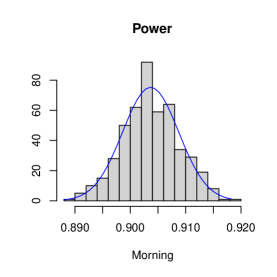
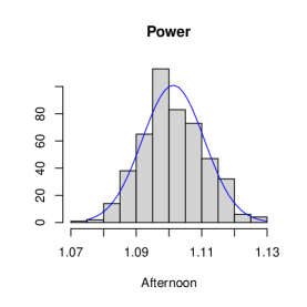
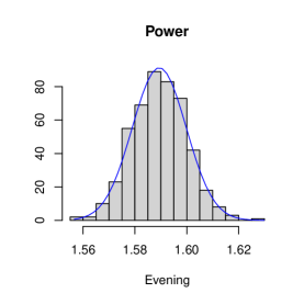
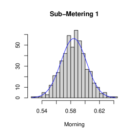
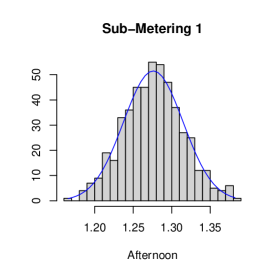
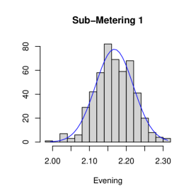
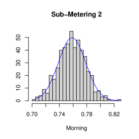
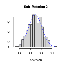
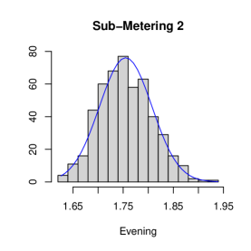
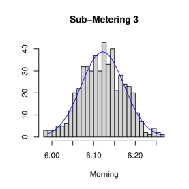
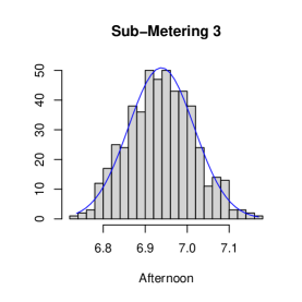
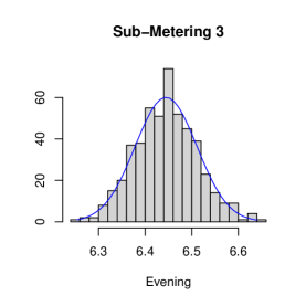
Figure 6: Bootstrap histograms of linear regression models with $a=0.2$.

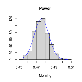
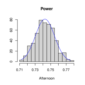
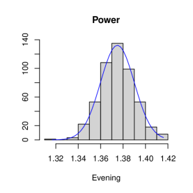
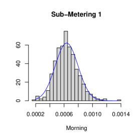
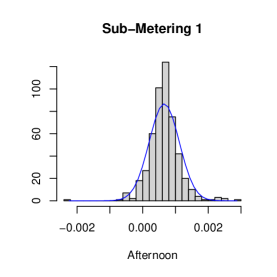
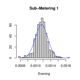
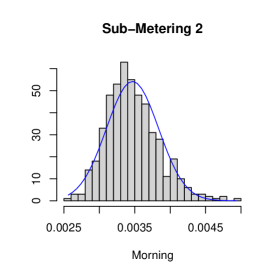
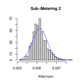
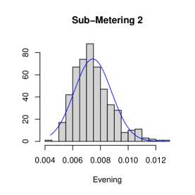
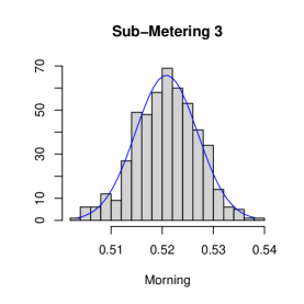
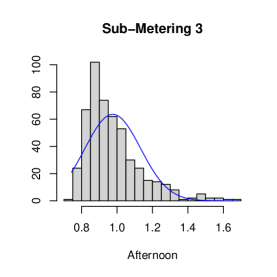
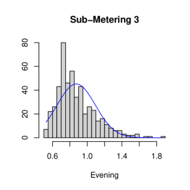
Figure 7: Bootstrap histograms of LAD regression models with $a=0.2$.

References

- Agarwal and Duchi, (2012) Agarwal, A. and Duchi, J. C. (2012). The generalization ability of online algorithms for dependent data. IEEE Transactions on Information Theory, 59(1):573–587.
- Bottou et al., (2018) Bottou, L., Curtis, F. E., and Nocedal, J. (2018). Optimization methods for large-scale machine learning. Siam Review, 60(2):223–311.
- Bradley, (2005) Bradley, R. C. (2005). Basic Properties of Strong Mixing Conditions. A Survey and Some Open Questions. Probability Surveys, 2(none):107 – 144.
- (4) Chen, E. Y., Song, R., and Jordan, M. I. (2022a). Reinforcement learning with heterogeneous data: estimation and inference. arXiv preprint arXiv:2202.00088.
- Chen et al., (2021) Chen, H., Lu, W., and Song, R. (2021). Statistical inference for online decision making via stochastic gradient descent. Journal of the American Statistical Association, 116(534):708–719.
- (6) Chen, X., Lai, Z., Li, H., and Zhang, Y. (2022b). Online statistical inference for contextual bandits via stochastic gradient descent. arXiv preprint arXiv:2212.14883.
- Chen et al., (2020) Chen, X., Lee, J. D., Tong, X. T., and Zhang, Y. (2020). Statistical inference for model parameters in stochastic gradient descent. The Annals of Statistics, 48(1):251–273.
- Cole-Rhodes et al., (2003) Cole-Rhodes, A. A., Johnson, K. L., LeMoigne, J., and Zavorin, I. (2003). Multiresolution registration of remote sensing imagery by optimization of mutual information using a stochastic gradient. IEEE transactions on image processing, 12(12):1495–1511.
- Dalal et al., (2018) Dalal, G., Szörényi, B., Thoppe, G., and Mannor, S. (2018). Finite sample analyses for td (0) with function approximation. In Proceedings of the AAAI Conference on Artificial Intelligence, volume 32.
- Deng et al., (2020) Deng, W., Lin, G., and Liang, F. (2020). A contour stochastic gradient langevin dynamics algorithm for simulations of multi-modal distributions. In Larochelle, H., Ranzato, M., Hadsell, R., Balcan, M., and Lin, H., editors, Advances in Neural Information Processing Systems, volume 33, pages 15725–15736. Curran Associates, Inc.
- Ding et al., (2021) Ding, J., Huh, W. T., and Rong, Y. (2021). Feature-based nonparametric inventory control with censored demand. Available at SSRN 3803777.
- Dua and Graff, (2017) Dua, D. and Graff, C. (2017). UCI machine learning repository.
- Fan and Yao, (2003) Fan, J. and Yao, Q. (2003). Nonlinear Time Series: Nonparametric and Parametric Methods. Springer Science Business Media, LLC.
- Fang et al., (2018) Fang, Y., Xu, J., and Yang, L. (2018). Online bootstrap confidence intervals for the stochastic gradient descent estimator. Journal of Machine Learning Research, 19(1):3053–3073.
- Ferguson, (2017) Ferguson, T. S. (2017). A course in large sample theory. Routledge.
- Fox et al., (2016) Fox, R., Pakman, A., and Tishby, N. (2016). Taming the noise in reinforcement learning via soft updates. In Proceedings of the Thirty-Second Conference on Uncertainty in Artificial Intelligence, UAI’16, page 202–211, Arlington, Virginia, USA. AUAI Press.
- Gower et al., (2019) Gower, R. M., Loizou, N., Qian, X., Sailanbayev, A., Shulgin, E., and Richtárik, P. (2019). Sgd: General analysis and improved rates. In In Proceedings of International Conference on Machine Learning. PMLR.
- Jérôme, (2005) Jérôme, L. (2005). A central limit theorem for robbins monro algorithms with projections. preprint on webpage at https://cermics.enpc.fr/cermics-rapports-recherche/2005/CERMICS-2005/CERMICS-2005-285.pdf.
- Khan et al., (2019) Khan, Z. A., Chaudhary, N. I., and Zubair, S. (2019). Fractional stochastic gradient descent for recommender systems. Electronic Markets, 29(2):275–285.
- Klein et al., (2009) Klein, S., Pluim, J. P., Staring, M., and Viergever, M. A. (2009). Adaptive stochastic gradient descent optimisation for image registration. International journal of computer vision, 81(3):227–239.
- Kuczmaszewska, (2011) Kuczmaszewska, A. (2011). On the strong law of large numbers for -mixing and -mixing random variables. Acta Mathematica Hungarica, 132(1-2):174–189.
- (22) Lee, S., Liao, Y., Seo, M. H., and Shin, Y. (2022a). Fast and robust online inference with stochastic gradient descent via random scaling. In Proceedings of the AAAI Conference on Artificial Intelligence, volume 36, pages 7381–7389.
- (23) Lee, S., Liao, Y., Seo, M. H., and Shin, Y. (2022b). Fast inference for quantile regression with millions of observations. arXiv preprint arXiv:2209.14502.
- Liang et al., (2007) Liang, F., Liu, C., and Carroll, R. J. (2007). Stochastic approximation in monte carlo computation. Journal of the American Statistical Association, 102(477):305–320.
- Liu et al., (2022) Liu, R., Yuan, M., and Shang, Z. (2022). Online statistical inference for parameters estimation with linear-equality constraints. Journal of Multivariate Analysis, 191:105017.
- Ma et al., (2022) Ma, S., Chen, Z., Zhou, Y., Ji, K., and Liang, Y. (2022). Data sampling affects the complexity of online sgd over dependent data. arXiv preprint arXiv:2204.00006.
- Melo et al., (2008) Melo, F. S., Meyn, S. P., and Ribeiro, M. I. (2008). An analysis of reinforcement learning with function approximation. In Proceedings of the 25th international conference on Machine learning, pages 664–671.
- Nemirovski et al., (2009) Nemirovski, A., Juditsky, A., Lan, G., and Shapiro, A. (2009). Robust stochastic approximation approach to stochastic programming. SIAM Journal on Optimization, 19(4):1574–1609.
- Pelletier, (2000) Pelletier, M. (2000). Asymptotic almost sure efficiency of averaged stochastic algorithms. SIAM Journal on Control and Optimization, 39(1):49–72.
- Polyak, (1990) Polyak, B. T. (1990). New method of stochastic approximation type. Automation and remote control, 51(7 pt 2):937–946.
- Polyak and Juditsky, (1992) Polyak, B. T. and Juditsky, A. B. (1992). Acceleration of stochastic approximation by averaging. SIAM journal on Control and Optimization, 30(4):838–855.
- Qu and Wierman, (2020) Qu, G. and Wierman, A. (2020). Finite-time analysis of asynchronous stochastic approximation and q-learning. In Conference on Learning Theory, pages 3185–3205. PMLR.
- Ramprasad et al., (2022) Ramprasad, P., Li, Y., Yang, Z., Wang, Z., Sun, W. W., and Cheng, G. (2022). Online bootstrap inference for policy evaluation in reinforcement learning. Journal of the American Statistical Association, pages 1–14.
- Robbins and Monro, (1951) Robbins, H. and Monro, S. (1951). A stochastic approximation method. Annals of Mathematical Statistics, 22(3):400–407.
- Robbins and Siegmund, (1971) Robbins, H. and Siegmund, D. (1971). A convergence theorem for non negative almost supermartingales and some applications. In Rustagi, J. S., editor, Optimizing Methods in Statistics, pages 233–257. Academic Press.
- Ruppert, (1988) Ruppert, D. (1988). Efficient estimations from a slowly convergent robbins-monro process. Technical report, Cornell University Operations Research and Industrial Engineering.
- Shi et al., (2021) Shi, C., Zhang, S., Lu, W., and Song, R. (2021). Statistical inference of the value function for reinforcement learning in infinite horizon settings. Journal of the Royal Statistical Society. Series B: Statistical Methodology. In Press.
- Shi et al., (2022) Shi, C., Zhu, J., Ye, S., Luo, S., Zhu, H., and Song, R. (2022). Off-policy confidence interval estimation with confounded markov decision process. Journal of the American Statistical Association, pages 1–12.
- Shi et al., (2020) Shi, X., He, Q., Luo, X., Bai, Y., and Shang, M. (2020). Large-scale and scalable latent factor analysis via distributed alternative stochastic gradient descent for recommender systems. IEEE Transactions on Big Data.
- Su and Zhu, (2018) Su, W. J. and Zhu, Y. (2018). Uncertainty quantification for online learning and stochastic approximation via hierarchical incremental gradient descent. arXiv preprint arXiv:1802.04876.
- Xu et al., (2019) Xu, T., Zou, S., and Liang, Y. (2019). Two time-scale off-policy td learning: Non-asymptotic analysis over markovian samples. Advances in Neural Information Processing Systems, 32.
- Yokoyama, (1980) Yokoyama, R. (1980). Moment bounds for stationary mixing sequences. Zeitschrift für Wahrscheinlichkeitstheorie und verwandte Gebiete, 52(1):45–57.
- Yu, (1994) Yu, B. (1994). Rates of convergence for empirical processes of stationary mixing sequences. Annals of Probability, pages 94–116.
- Yuan et al., (2021) Yuan, H., Luo, Q., and Shi, C. (2021). Marrying stochastic gradient descent with bandits: Learning algorithms for inventory systems with fixed costs. Management Science, 67(10):6089–6115.