Towards Computationally Efficient Responsibility Attribution in Decentralized Partially Observable MDPs

Abstract.

Responsibility attribution is a key concept of accountable multi-agent decision making. Given a sequence of actions, responsibility attribution mechanisms quantify the impact of each participating agent to the final outcome. One such popular mechanism is based on actual causality, and it assigns (causal) responsibility based on the actions that were found to be pivotal for the considered outcome. However, the inherent problem of pinpointing actual causes and consequently determining the exact responsibility assignment has shown to be computationally intractable. In this paper, we aim to provide a practical algorithmic solution to the problem of responsibility attribution under a computational budget. We first formalize the problem in the framework of Decentralized Partially Observable Markov Decision Processes (Dec-POMDPs) augmented by a specific class of Structural Causal Models (SCMs). Under this framework, we introduce a Monte Carlo Tree Search (MCTS) type of method which efficiently approximates the agents’ degrees of responsibility. This method utilizes the structure of a novel search tree and a pruning technique, both tailored to the problem of responsibility attribution. Other novel components of our method are (a) a child selection policy based on linear scalarization and (b) a backpropagation procedure that accounts for a minimality condition that is typically used to define actual causality. We experimentally evaluate the efficacy of our algorithm through a simulation-based test-bed, which includes three team-based card games.

1. Introduction

One of the well known Gedankenexperimente in the AI literature on actual causality and responsibility attribution is the story of Suzy and Billy. As J. Y. Halpern describes it in his book on Actual Causality Halpern (2016), the story goes as follows:

“Suzy and Billy both pick up rocks and throw them at a bottle. Suzy’s rock gets there first, shattering the bottle. Because both throws are perfectly accurate, Billy’s would have shattered the bottle had it not been preempted by Suzy’s throw.”

Who is to be held responsible for the bottle being shattered? As the curious reader may have noticed, the conceptual challenge of attributing responsibility for this outcome lies in the fact that the outcome would not have changed had Suzy not thrown her rock. Needless to say, there are a plethora of other examples from moral philosophy that challenge human intuition on how responsibility should be ascribed, including Bogus Prevention Hiddleston (2005), Marksmen Halpern (2016), Arsonists Halpern and Pearl (2005), and Bystanders Halpern and Hitchcock (2011).

Much of the (recent) work in moral philosophy and AI has focused on resolving these conceptual challenges utilizing different formal frameworks Baier et al. (2021a, b); Alechina et al. (2020); Yazdanpanah et al. (2019). Often, perhaps unsurprisingly, these works Chockler and Halpern (2004); Halpern and Kleiman-Weiner (2018); Triantafyllou et al. (2022) take as a starting point the framework of actual causality based on Structural Causal Models (SCMs) Pearl (1995). Given a specific scenario, approaches that utilize this framework typically first pinpoint actions that were pivotal to the outcome of that scenario. It is also not hard to see the importance of these works for accountable AI systems. Consider, for example, a semi-autonomous vehicle, and let Suzy be the auto-pilot of this vehicle, Billy be the human driver that oversees the autopilot, and the shattered bottle be the pedestrian injured in an accident caused by the vehicle.

However, real-world scenarios are often much more complex than the aforementioned examples from moral philosophy capture. In order to operationalize responsibility attribution for automated, yet accountable decision making systems it is important to ground it in a framework that is general enough to capture the nuances of real-world decision making settings. This has recently been recognized by Triantafyllou et al. (2022), who study the problem of actual causality and responsibility attribution in Decentralized Partially Observable Markov Decision Processes (Dec-POMDPs) – a rather general framework for multi-agent sequential decision making under uncertainty. However, while Triantafyllou et al. (2022) show how to combine Dec-POMDPs with SCMs to enable causal reasoning, they still primarily focus on challenges related to defining actual causality and designing responsibility attribution mechanisms. In contrast, in this paper we focus on the fact that the problem of inferring actual causes, and consequently attributing causal responsibility, is known to have high computational complexity Eiter and Lukasiewicz (2002); Aleksandrowicz et al. (2017); Halpern (2015). Since determining the exact responsibility assignment is then intractable, we ask the following question: “Can we design an efficient procedure for approximately ascribing responsibility in Dec-POMDPs?”

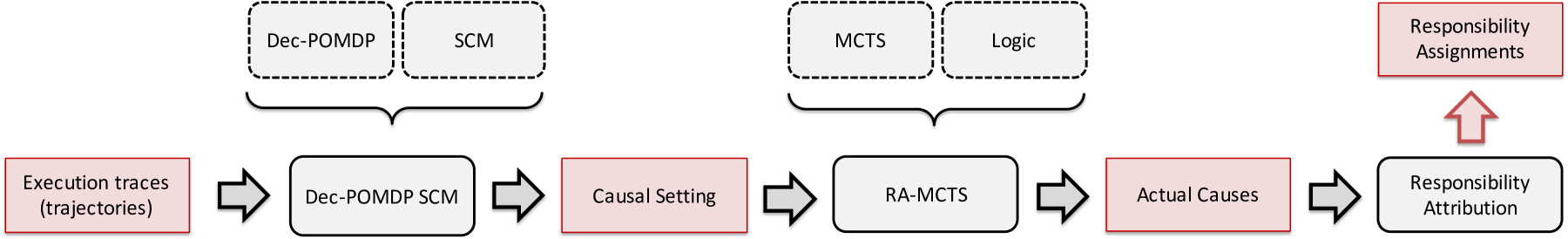
Figure 1. The figure provides an overview of our approach to responsibility attribution in Dec-POMDPs. Based on received execution traces, that is the agents’ trajectories, our approach first aims to infer the underlying context under which these decisions were made. To do so we utilize Dec-POMDP SCMs – a framework introduced in Triantafyllou et al. (2022) that combines Dec-POMDPs and SCMs. The context in our case models randomness/noise, and together with the underlying causal model forms the causal setting. The next step is to apply an MCTS type of search to infer actual causes that are consistent with the definition of actual causality introduced in Triantafyllou et al. (2022). This search method is formally specified in a language that is an extension of propositional logic. In order to determine the agents’ degrees of responsibilities, we apply the responsibility attribution method of Chockler and Halpern (2004) over the actual causes found by the search. In cases where the underlying context cannot be exactly inferred we use posterior inference over possible contexts. More specifically, we first draw samples from the posterior over possible contexts, and then repeat the process described above for each sampled context. Agents are assigned the average degrees of responsibility over all samples.

We propose an algorithmic framework for approximating responsibility assignments under a computational budget. Having a bounded budget is important for complex systems, where brute-force approaches do not work Halpern (2016); Ibrahim et al. (2019). The example scenarios range from autonomous public transit systems and system controllers, such as traffic light controllers (TLC), to multi-agent cooperative systems, such as warehouse robots. For an extended discussion on the application scenario of TLC see Appendix B.

Fig. 1 provides an overview of our algorithmic approach. We recognize two main challenges that this approach has to overcome. The first one is a statistical challenge and is related to the fact that in practice the context under which an outcome of interest is generated cannot be always inferred. As explained in Fig. 1, to make responsibility attribution feasible in such cases, we use posterior inference over the possible values of the underlying context. The second challenge is a computational one and it is related to the computational complexity of identifying actual causes. We tackle this challenge by applying a Monte Carlo Tree Search (MCTS) type of method tailored to the problem of finding actual causes. As we show in this paper, our approach significantly outperforms baselines in terms of approximating the “ideal” responsibility assignments, obtained under no uncertainty and unlimited computational budget. Our contributions are primarily related to the design and experimental evaluation of this algorithmic framework, and they include:

• A novel search tree tailored to the tasks of pinpointing actual causes and attributing responsibility.

• A novel pruning technique that utilizes the structural properties of both the actual causality definition of Triantafyllou et al. (2022) and the responsibility attribution mechanism of Chockler and Halpern (2004).

• Responsibility Attribution-MCTS (RA-MCTS), a new search method for efficiently finding actual causes under a given causal setting. Compared to standard MCTS, the main novel components of RA-MCTS are in its simulation phase, evaluation function, child selection policy, and backpropagation phase.

• Experimental test-bed for evaluating the efficacy of RA-MCTS. The test-bed is based on three card games, Euchre Wright (2001), Spades Cohensius et al. (2019), and a team variation of the game Goofspiel Ross (1971). We deem the test-bed to be generally useful for studying actual causality and responsibility attribution in multi-agent sequential decision making. Our experimental results show that RA-MCTS almost always outperforms baselines, such as random search, brute-force search, or modifications of RA-MCTS. Our results also show that in cases where the underlying context cannot be exactly inferred, computing a good approximation of the “ideal” responsibility assignment might not be possible, even under unlimited computational budget. This can happen when the posterior distribution over the possible contexts is not informative enough.

1.1. Additional Related Work

This paper is related to works on responsibility and blame attribution in multi-agent decision making Baier et al. (2021a, b); Yazdanpanah et al. (2019); Triantafyllou et al. (2021); Halpern and Kleiman-Weiner (2018); Friedenberg and Halpern (2019).

To the best of our knowledge, there is no prior work on developing general algorithmic approaches on efficiently computing degrees of causal responsibility. The closest we could find, are domain-specific applications of the Chockler and Halpern responsibility approach Chockler and Halpern (2004) in program verification Chockler et al. (2008b, a). Chapter $8$ of Halpern (2016) provides a general overview of such applications. Additionally, to our knowledge, the only general algorithmic approach on determining causality, and subsequently responsibility attribution, is that of Ibrahim et al. (2019). Their approach on checking actual causality utilizes SAT solvers and thus is significantly different than ours. They also restrict their focus to binary models, as opposed to ours which considers categorical variables.

The only other work that has used the same framework as the one used in this paper is that of Triantafyllou et al. (2022). Close to our work in this aspect, Buesing et al. (2018) and Oberst and Sontag (2019) have considered a combination of SCMs with POMDPs. Tsirtsis et al. (2021) utilize a connection between SCMs and MDPs to generate counterfactual explanations for sequential decision making.

This paper is also related to a line of work which introduces variants of MCTS that apply to specific domains. For instance, Schadd et al. (2008) and Bjornsson and Finnsson (2009) propose modifications to MCTS in order to adapt it to single-player games. We refer the interested reader to Browne et al. (2012) for more such examples.

2. Framework and Background

In this section, we first give an overview of a formal framework which allows us to study responsibility attribution in the context of multi-agent sequential decision making. This framework is adopted from Triantafyllou et al. (2022), and relies on decentralized partially observable Markov decision processes (Dec-POMDPs) Bernstein et al. (2002); Oliehoek and Amato (2016) and structural causal models (SCMs) Pearl (2009); Peters et al. (2017). Next, we provide the necessary background on actual causality and responsibility attribution. Finally, we state the responsibility attribution problem and highlight its main algorithmic challenges.

2.1. Dec-POMDPs

The first component of this framework are Dec-POMDPs with $n$ agents; state space $\mathcal{S}$; joint action space $\mathcal{A}=\times_{i=1}^{n}\mathcal{A}_{i}$, where $\mathcal{A}_{i}$ is the action space of agent $i$; transition probability function $P:\mathcal{S}\times\mathcal{A}\rightarrow\Delta(\mathcal{S})$; joint observation space $\mathcal{O}=\times_{i=1}^{n}\mathcal{O}_{i}$, where $\mathcal{O}_{i}$ is the observation space of agent $i$; observation probability function $\Omega:\mathcal{S}\rightarrow\Delta(\mathcal{O})$; finite time horizon $T$; initial state distribution $\sigma$. Here $\Delta$ denotes the probability simplex. For ease of notation, rewards are considered to be part of observations.

Each agent $i$ is modeled with an information state space $\mathcal{I}_{i}$; decision making policy $\pi_{i}:\mathcal{I}_{i}\rightarrow\Delta(\mathcal{A}_{i})$; information probability function $Z_{i}:\mathcal{I}_{i}\times\mathcal{A}_{i}\times\mathcal{O}_{i}\rightarrow\mathcal{I}_{i}$; initial information probability function $Z_{i,0}:\mathcal{O}_{i}\rightarrow\mathcal{I}_{i}$. We denote with $\pi_{i}(a_{i}|\imath_{i})$ agent $i$’s probability of taking action $a_{i}$ given information state $\imath_{i}$, and with $\pi$ the collection of all agents’ policies, i.e., the agents’ joint policy.

We assume spaces $\mathcal{S}$, $\mathcal{A}$, $\mathcal{O}$ and $\mathcal{I}_{i}$ to be finite and discrete.

2.2. Dec-POMDPs and Structural Causal Models

In order to reason about actual causality and responsibility attribution in multi-agent sequential decision making Triantafyllou et al. (2022) view Dec-POMDPs as SCMs. More specifically, given a Dec-POMDP $\mathcal{M}=(\mathcal{S},\{1,...,n\},\mathcal{A},P,\mathcal{O},\Omega,T,\sigma)$ and a model $m_{i}=(\mathcal{I}_{i},\pi_{i},Z_{i},Z_{i,0})$ for each agent $i$, they construct a SCM $\mathcal{C}$, which they refer to as Dec-POMDP SCM. Under $\mathcal{C}$ functions $P$, $\Omega$, $\{Z_{i}\}_{i\in\{1,...,n\}}$ and $\{\pi_{i}\}_{i\in\{1,..,n\}}$ are parameterized as follows

$$S_{t}=g_{S_{t}}(S_{t-1},A_{t-1},U_{S_{t}}),\quad O_{t}=g_{O_{t}}(S_{t},U_{O_{t}}),$$

$$I_{i,t}=g_{I_{i,t}}(I_{i,t-1},A_{i,t-1},O_{i,t},U_{I_{i,t}}),\quad A_{i,t}=g_{A_{i,t}}(I_{i,t},U_{A_{i,t}}),$$ (1)

where $g_{S_{t}}$, $g_{O_{t}}$, $g_{I_{i,t}}$ and $g_{A_{i,t}}$ are deterministic functions, and $U_{S_{t}}$, $U_{O_{t}}$, $U_{I_{i,t}}$ and $U_{A_{i,t}}$ are independent noise variables with dimensions $|\mathcal{S}|$, $|\mathcal{O}|$, $|\mathcal{I}_{i}|$ and $|\mathcal{A}_{i}|$, respectively.

Following SCM terminology Pearl (2009), we refer to state variables $S_{t}$, observation variables $O_{t}$, information variables $I_{i,t}$ and action variables $A_{i,t}$ as the endogenous variables of $\mathcal{C}$. Furthermore, we call noise variables $U$ the exogenous variables of $\mathcal{C}$ and a setting $\@vec{u}$ of $U$ context. Note that given a context $\@vec{u}$ one can compute the value of any endogenous variable in $\mathcal{C}$ by consecutively solving equations in (2.2), also called structural equations. Therefore, a Dec-POMDP SCM-context pair $(\mathcal{C},\@vec{u})$, also called causal setting, specifies a unique trajectory $\tau=\{(s_{t},a_{t})\}_{t=0}^{T-1}$.

Another well-known notion in causality that is important for our analysis is that of interventions Pearl (1995). An intervention $A_{i,t}\leftarrow a^{\prime}_{i}$ on SCM $\mathcal{C}$ is performed by replacing $g_{A_{i,t}}(I_{i,t},U_{A_{i},t})$ in Eq. (2.2) with $a^{\prime}_{i}$, also called the counterfactual action of the intervention. We denote the resulting SCM by $\mathcal{C}^{A_{i,t}\leftarrow a^{\prime}_{i}}$. If one has knowledge over $\mathcal{C}$ as well as the context $\@vec{u}$ under which a trajectory $\tau$ was generated, they can efficiently compute the counterfactual outcome of that trajectory under some intervention $A_{i,t}\leftarrow a^{\prime}_{i}$ on $\mathcal{C}$. This can be done by simply generating the counterfactual trajectory $\tau^{cf}$ that corresponds to the causal setting $(\mathcal{C}^{A_{i,t}\leftarrow a^{\prime}_{i}},\@vec{u})$. In other words, they can predict exactly what would have happened in that scenario had agent $i$ taken action $a^{\prime}_{i}$ instead of $a_{i,t}$. However, the true underlying SCM $\mathcal{C}$ or context $\@vec{u}$ are not always available in practice. Following a standard modeling approach Triantafyllou et al. (2022); Lorberbom et al. (2021); Tsirtsis et al. (2021), we restrict our focus on a specific class of SCMs, the Gumbel-Max SCMs, introduced by Oberst and Sontag (2019). More details on Gumbel-Max SCMs and how they can be integrated in the Dec-POMDP SCM framework, can be found in Appendix C.

2.3. Actual Causality

Next, we present a language for reasoning about actual causality in (Dec-POMDP) SCMs Halpern (2016). Let $\mathcal{C}$ be a Dec-POMDP SCM. A primitive event in $C$ is any formula of the form $V=v$, where $V$ is an endogenous variable of $\mathcal{C}$ and $v$ is a valid value of $V$. We say that a Boolean combination of primitive events constitutes an event. Given a context $\@vec{u}$ and an event $\phi$, we write $(\mathcal{C},\@vec{u})\models\phi$ to denote that $\phi$ takes place in the causal setting $(\mathcal{C},\@vec{u})$. Furthermore, for a set of interventions $\@vec{A}\leftarrow\@vec{a}^{\prime}$ on $\mathcal{C}$, we write $(\mathcal{C},\@vec{u})\models[\@vec{A}\leftarrow\@vec{a}^{\prime}]\phi$, if $(\mathcal{C}^{\@vec{A}\leftarrow\@vec{a}^{\prime}},\@vec{u})\models\phi$. For example, let $\tau=\{(s_{t},a_{t})\}_{t=0}^{T-1}$ be the trajectory that corresponds to $(\mathcal{C},\@vec{u})$. Consider the counterfactual scenario in which agent $i$ takes action $a_{i}^{\prime}$ instead of $a_{i,t}$ in $\tau$, and the process transitions to state $s$ at $t+1$. This can be expressed by

$$(\mathcal{C},\@vec{u})\models[A_{i,t}\leftarrow a_{i}^{\prime}](S_{t+1}=s).$$

In the context of Dec-POMDP SCMs actual causality is related to the process of pinpointing agents’ actions that were critical for $\phi$ to happen in $(\mathcal{C},\@vec{u})$. In this paper, we adopt the actual cause definition proposed by Triantafyllou et al. (2022). Their definition utilizes the agents’ information states in order to explicitly account for the temporal dependencies between agents’ actions.

Definition .

(Actual Cause) $\@vec{A}=\@vec{a}$ is an actual cause of the event $\phi$ in $(\mathcal{C},\@vec{u})$under the contingency $\@vec{W}=\@vec{w}^{\prime}$ if the following conditions hold:

1. $(\mathcal{C},\@vec{u})\models(\@vec{A}=\@vec{a})$ and $(\mathcal{C},\@vec{u})\models\phi$

2. There is a setting $\@vec{a}^{\prime}$ of the variables in $\@vec{A}$, such that

   $$(\mathcal{C},\@vec{u})\models[\@vec{A}\leftarrow\@vec{a}^{\prime},\@vec{W}\leftarrow\@vec{w}^{\prime}]\neg\phi$$

3. $\@vec{A}\cup\@vec{W}$ is minimal w.r.t. conditions AC1 and AC2

4. For every agent $i$ and time-step $t$ such that $A_{i,t}\in\@vec{A}$ and $(\mathcal{C},\@vec{u})\models(I_{i,t}=\imath_{i,t})$, it holds that

   $$(\mathcal{C},\@vec{u})\models[\@vec{A}\leftarrow\@vec{a}^{\prime},\@vec{W}\leftarrow\@vec{w}^{\prime}](I_{i,t}=\imath_{i,t})$$

5. For every agent $i$ and time-step $t$ such that $A_{i,t}\in\@vec{W}$ and $(\mathcal{C},\@vec{u})\models(I_{i,t}=\imath_{i,t})$, it holds that

   $$(\mathcal{C},\@vec{u})\models[\@vec{A}\leftarrow\@vec{a}^{\prime},\@vec{W}\leftarrow\@vec{w}^{\prime}]\neg(I_{i,t}=\imath_{i,t})$$

We say that the tuple $(\@vec{W},\@vec{w}^{\prime},\@vec{a}^{\prime})$ is a witness of $\@vec{A}=\@vec{a}$ being an actual cause of $\phi$ in $(\mathcal{C},\@vec{u})$.

AC1 requires that both $\@vec{A}=\@vec{a}$ and $\phi$ happened in $(\mathcal{C},\@vec{u})$. AC2 implies that $\phi$ would not have occurred under the interventions $\@vec{A}\leftarrow\@vec{a}^{\prime}$ and $\@vec{W}\leftarrow\@vec{w}^{\prime}$ on $(\mathcal{C},\@vec{u})$. AC3 is a minimality condition, which ensures that there are no subsets $\@vec{A}^{\prime}$ and $\@vec{W}^{\prime}$ of $\@vec{A}$ and $\@vec{W}$, and setting $\@vec{w}^{\prime\prime}$ of $\@vec{W}^{\prime}$, such that $\@vec{A}^{\prime}=\@vec{a}^{\prime}$ and $\@vec{W}^{\prime}=\@vec{w}^{\prime\prime}$ satisfy AC1 and AC2, where $\@vec{a}^{\prime}$ is the restriction of $\@vec{a}$ to the variables of $\@vec{A}$. AC4 (resp. AC5) requires that the information states which correspond to the action variables in $\@vec{A}$ (resp. $\@vec{W}$) have the same (resp. different) values in the counterfactual scenario $(\mathcal{C}^{\@vec{A}\leftarrow\@vec{a}^{\prime},\@vec{W}\leftarrow\@vec{w}^{\prime}},\@vec{u})$ and the actual scenario $(\mathcal{C},\@vec{u})$. We say that a conjunct of an actual cause $\@vec{A}=\@vec{a}$ constitutes a part of that cause. If for some $\@vec{A}=\@vec{a}$ and $\@vec{W}=\@vec{w}^{\prime}$ conditions AC1, AC2, AC4 and AC5 hold we say that $\@vec{A}=\@vec{a}$ is a candidate actual cause of $\phi$ in $(\mathcal{C},\@vec{u})$ under the contingency $\@vec{W}=\@vec{w}^{\prime}$. We also say that a set of interventions $\@vec{X}\leftarrow\@vec{x}^{\prime}$ constitutes an (candidate) actual cause-witness pair according to Definition 2.3 if there exists such a pair $(\@vec{A}=\@vec{a},(\@vec{W},\@vec{w}^{\prime},\@vec{a}^{\prime}))$, where $\@vec{X}=\@vec{A}\cup\@vec{W}$, and $\@vec{a}^{\prime}$ and $\@vec{w}^{\prime}$ are the projections of $\@vec{x}^{\prime}$ in $\@vec{A}$ and $\@vec{W}$, respectively.

2.4. Responsibility Attribution

Responsibility attribution is a concept closely related to actual causality, which aims to determine the extent to which agents’ actions were pivotal for some outcome. In this paper, we adopt a responsibility attribution approach which was first introduced by Chockler and Halpern (2004), and then adapted by Triantafyllou et al. (2022) to the setting of Dec-POMDP SCMs. Given a causal setting $(\mathcal{C},\@vec{u})$ and an event $\phi$, the Chockler and Halpern approach (henceforth CH) uses the following function to determine an agent $i$’s degree of responsibility for $\phi$ in $(\mathcal{C},\@vec{u})$ relative to a set of interventions $\@vec{X}\leftarrow\@vec{x}^{\prime}$ on $\mathcal{C}$ and an actual causality definition $\mathcal{D}$

$$dr_{i}((\mathcal{C},\@vec{u}),\phi,\@vec{X}\leftarrow\@vec{x}^{\prime},\mathcal{D})=\frac{m_{i}}{|\@vec{X}|},$$ (2)

where $m_{i}$ is computed as follows. If $\@vec{X}\leftarrow\@vec{x}^{\prime}$ constitutes an actual cause-witness pair $(\@vec{A}=\@vec{a},(\@vec{W},\@vec{w}^{\prime},\@vec{a}^{\prime}))$ of $\phi$ in $(\mathcal{C},\@vec{u})$ according to $\mathcal{D}$, then $m_{i}$ denotes the number of $i$’s action variables in $\@vec{A}$. Otherwise, $m_{i}$ is $0$. In this paper, an agent’s degree of responsibility according to the CH approach is computed as follows.

Definition .

(CH) Consider a causal setting $(\mathcal{C},\@vec{u})$ and an event $\phi$ such that $(\mathcal{C},\@vec{u})\models\phi$. With $\mathcal{D}$ being Definition 2.3, an agent $i$’s degree of responsibility for $\phi$ in $(\mathcal{C},\@vec{u})$ is equal to the maximum value $dr_{i}((\mathcal{C},\@vec{u}),\phi,\@vec{X}\leftarrow\@vec{x}^{\prime},\mathcal{D})$ over all possible sets of interventions $\@vec{X}\leftarrow\@vec{x}^{\prime}$ on $\mathcal{C}$.

The CH definition captures some key ideas of responsibility attribution. First, an agent’s degree of responsibility depends on the size of an actual cause $\@vec{A}=\@vec{a}$ the agent participates in. Second, it depends on the amount of participation the agent has in that cause. Finally, it depends on the size of the smallest contingency of $\@vec{A}=\@vec{a}$, i.e., the minimum number of interventions that need to be performed on $\mathcal{C}$ in order to make $\phi$ counterfactually depend on $\@vec{A}$.

2.5. Problem Statement and Challenges

Given a trajectory $\tau$ generated by causal setting $(\mathcal{C},\@vec{u})$, the general problem we are interested in is computing the agents’ degrees of responsibility for the final outcome $\phi^{\tau}$ of $\tau$. In this paper, we focus on two main challenges of this problem. The first one is related to the computational complexity of the problem. The second one has to do with the fact that in practice context $\@vec{u}$ might not be known.

In order to address the first challenge, we view responsibility attribution as a multi-objective search problem with limited computational resources. An algorithmic solution to this problem should find a set of interventions, for each agent, that maximizes the function in Eq. (2). The pipeline we consider for such algorithms can be summarized as follows. First, the algorithm searches for sets of interventions that constitute actual cause-witness pairs of the outcome $\phi^{\tau}$. Next, based on the found actual cause-witness pairs the algorithm computes the responsibility assignment. A natural question that arises is how to choose which intervention sets to evaluate before the computational budget is exhausted. We believe that the answer to this question lies in the structural properties of Definitions 2.3 and 2.4 (Sections 3.1-3.3). Another question related to this problem is how to recognize if a set of interventions is in fact an actual cause-witness pair. Even though it is easy to infer whether a set of interventions constitutes a candidate actual cause-witness pair of $\phi^{\tau}$ when $(\mathcal{C},\@vec{u})$ is known, it is impossible to know if it is minimal, i.e., if it satisfies condition AC3, unless all of its subsets are first checked for AC1 and AC2. Despite that, there are countermeasures that one can implement to reduce the negative impact that AC3 might have on the search process (Section 3.3).

To address the second challenge, we view responsibility attribution as an inference problem. Our approach is to build on the above mentioned search algorithm, and by using posterior inference design a mechanism that can efficiently estimate responsibility assignments under context uncertainty (Section 3.4).

3. Algorithmic Solution

In this section, we analyze our algorithmic solutions to the search and inference problems described in Section 2.5. First, we propose a novel search tree tailored to the tasks of pinpointing actual causes and attributing responsibility. Next, we propose a pruning technique that utilizes the structural properties of Definitions 2.3 and 2.4. We then propose RA-MCTS, a novel Monte Carlo Tree Search (MCTS) type of method for finding approximate responsibility assignments under limited computational budget. Finally, we propose an extension of RA-MCTS to the unknown context regime.

3.1. Search Tree

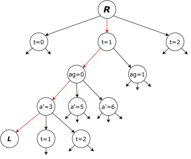
Figure 2. The red edges denote the path in our search tree, which corresponds to the intervention on the action of agent $0$ at time-step $1$ with counterfactual action $a^{\prime}=3$, $A_{0,1}\leftarrow 3$.

Fig. 2 illustrates an instantiation of our proposed search tree. Note that the tree is defined relative to the causal setting $(\mathcal{C},\@vec{u})$, that is, every state, observation, information state and action is deterministically computed by the structural equations of $\mathcal{C}$ together with context $\@vec{u}$ (see Eq. (2.2)). Nodes in this tree fall into one of $5$ categories. At the top of the tree, we have the Root node, where the time-step of the first intervention is selected. Nodes $t=0$, $t=1$ and $t=2$ in Fig. 2 correspond to their respective time-steps, and we call them TimeStep nodes. From a TimeStep node, the agent of the next intervention is picked. Nodes $ag=0$ and $ag=1$ correspond to agents $0$ and $1$, and they are categorized as Agent nodes. From an Agent node, the counterfactual action of the next intervention is chosen from the available options. More specifically, let $ag=i$ be the node where the search is currently on, and $t=t^{\prime}$ be that node’s parent. Let also $\@vec{X}\leftarrow\@vec{x}^{\prime}$ denote the current set of interventions encoded in $ag=i$. The available options from node $ag=i$ then include all the valid actions that $i$ could have taken at time-step $t^{\prime}$, except the action that it would have normally taken given the current set of interventions, i.e., the action determined by the causal setting $(\mathcal{C}^{\@vec{X}\leftarrow\@vec{x}^{\prime}},\@vec{u})$. Nodes $a^{\prime}=3$, $a^{\prime}=5$ and $a^{\prime}=6$ in Fig. 2 correspond to such counterfactual actions and they are characterized as Action nodes. From an Action node, search can either stop growing the intervention set, and hence transition to a Leaf node $L$ or continue by transitioning to the next TimeStep node. If search transitions to $L$, then the current set of interventions is evaluated. In case this set of interventions is found to change the final outcome $\phi^{\tau}$, it is added to the set of found candidate actual cause-witness pairs.

3.2. Pruning

Apart from its intuitive nature and computational efficiency (Section 4.3), the search tree of Fig. 2 also allows us to apply a number of effective pruning techniques. Pruning can take place at any point during the search and it is basically the process of removing branches from a tree that cannot possibly improve the output of the algorithm. In our setting, this means that a node needs not be further visited if it becomes apparent that the evaluation of any leaf node reachable from that node cannot in any way influence the final responsibility assignment. Our method prunes away a node (and all of its descendants) if any of the following conditions hold:

• It is a Leaf node that has already been evaluated.

• It is the closest ancestor Agent node of a Leaf node $L$, such that $L$’s encoded set of interventions $\@vec{X}\leftarrow\@vec{x}^{\prime}$ constitutes a candidate actual cause-witness pair. Note that the set of interventions encoded in any descendant of the pruned Agent node is either identical to $\@vec{X}\leftarrow\@vec{x}^{\prime}$ apart from its last counterfactual action, or its variable set is a superset of $\@vec{X}$, and hence it is non-minimal according to Definition 2.3.

• It is an Agent node whose encoded set of interventions is non-minimal w.r.t. to the current set of found candidate actual cause-witness pairs.

• It is a fully-expanded node with all of its children already pruned.

3.3. Responsibility Attribution Using Monte Carlo Tree Search (RA-MCTS)

The search algorithm we propose is based on the well-known Monte Carlo Tree Search (MCTS) method Browne et al. (2012). We refer to our algorithm as RA-MCTS because it is specific to the task of responsibility attribution. The main differences between RA-MCTS and standard MCTS Coulom (2006); Chaslot et al. (2008) are in their simulation phases, evaluation functions, child selection policies and backpropagation phases.

Simulation Phase. At each iteration, the entire simulation path is added to the search tree. Although in applications of MCTS the tree is usually expanded by one node per iteration, this would not be optimal in our setting. Namely, under a fixed causal setting, the state transitions, observations generation and other such functions are deterministic. Hence, computing their values more than once is a waste of computational resources.

Evaluation Function. Whenever a Leaf node $L$ is visited during an iteration of (RA-)MCTS, a score is assigned to it and then backpropagated to all of its ancestors. Properly defining the function that determines that score, i.e., the evaluation function, is considered to be a critical ingredient of successfully applying MCTS methods. Considering the idiosyncrasy of our task, we design an evaluation function that returns a multi-dimensional score, as opposed to a single numerical value which is typically the case. More precisely, this evaluation function takes as input the set of interventions $\@vec{X}\leftarrow\@vec{x}^{\prime}$ encoded in $L$, and outputs a score vector $\@vec{r}$, of size $n+1$, which is defined as follows. For each agent $i\in\{1,...,n\}$, $r_{i}=dr_{i}((\mathcal{C},\@vec{u}),\phi^{\tau},\@vec{X}\leftarrow\@vec{x}^{\prime},\mathcal{D})$, where $\mathcal{D}$ denotes Definition 2.3. The $n+1$th value of $\@vec{r}$ is equal to the output of an environment specific function $q_{\mbox{env}}((\mathcal{C},\@vec{u}),\@vec{X}\leftarrow\@vec{x}^{\prime})$ which provides some additional information about the final outcome that corresponds to the causal setting $(\mathcal{C}^{\@vec{X}\leftarrow\@vec{x}^{\prime}},\@vec{u})$. For example, in a card game scenario we typically want to attribute responsibility to the members of the team that lost (outcome). Additional information that our search algorithm could benefit from in this scenario is how closer to or further from winning would the losing team get, had we intervened on some actions taken by its members. The purpose of $\@vec{r}$’s first $n$ values is to guide the search towards optimizing its main objective, i.e., approximating the agents’ degrees of responsibility. The role of the last value of $\@vec{r}$ is complementary, as it helps to identify areas which are promising for discovering new actual causes.

Child Selection Policy. Similar to standard MCTS, in RA-MCTS each node $v$ keeps track of two statistics, the number $N(v)$ of times it has been visited and the vector $\@vec{Q}(v)$, where $Q_{j}(v)$, with $j\in\{1,..,n+1\}$, is equal to the total score $r_{j}$ of all simulations that passed through that node. In order to transform $\@vec{Q}(v)$ into a scalar score value, the child selection policy of RA-MCTS follows a linear scalarization approach inspired by the Multi-Objective Multi-Armed Bandits (MO-MAB) literature Drugan and Nowe (2013); Tekin and Turğay (2018). At iteration $k$, a pre-defined weight $b_{k,j}$ is assigned to each value of $\@vec{Q}(v)$, where $\sum_{j\in\{1,...,n+1\}}b_{k,j}=1$. The linear scalarized value of $\@vec{Q}(v)$ at iteration $k$ is then defined as

$$f_{LS}(\@vec{Q}(v))=\sum_{j\in\{1,...,n+1\}}b_{k,j}\cdot Q_{j}(v).$$ (3)

After computing $f_{LS}(\@vec{Q}(v))$ for each child node $v$, our policy employs the UCB$1$ formula Auer et al. (2002); Kocsis and Szepesvári (2006) to select the next node in the path

$$v^{next}:=\operatorname*{arg\,max}_{v\in\mbox{children}}\frac{f_{LS}(\@vec{Q}(v))}{N(v)}+C\cdot\sqrt{\frac{\ln{N}}{N(v)}},$$ (4)

where $N$ is the parent node’s number of visitations and $C$ is the exploration parameter of RA-MCTS. Ties are broken randomly.

In our experiments, at every iteration $k$, we set $b_{k,n+1}:=B$, where $B\in[0,1)$ is a constant. Additionally, for $i=(k\;\mathrm{mod}\;n)$ we set $b_{k,i}:=1-B$, while every other weight $b_{k,j}$, with $j\notin\{i,n+1\}$, is set to $0$. As a result, the only simulated responsibility degrees that guide the search at iteration $k$ are those of agent $i$.

Backpropagation Phase. Note that as the set of found candidate actual cause-witness pairs grows during search, the intervention set encoded in a previously expanded Agent node $v$ might be evaluated as non-minimal when $v$ gets visited again. Whenever this happens, in addition to pruning $v$, we also backpropagate values $(-\@vec{Q}(v),-N(v))$ to its ancestors. This way, we completely erase the footprints of the pruned node from the rest of the tree. Therefore, by taking this measure our search method is no longer guided by scores of simulations that passed through $v$.

3.4. Estimating Responsibility Assignments under Context Uncertainty

Our analysis so far in this section, assumes context $\@vec{u}$ to be known. We now lift this assumption and propose our solution to the inference problem described in Section 2.5. We extend RA-MCTS in the following way. First, we draw $M$ Monte Carlo samples from the posterior $Pr(\@vec{u}|\tau)$, utilizing the procedure described in Section 3.4 of Oberst and Sontag (2019). Next, we compute for each agent $i$ its average degree of responsibility over all samples

$$\overline{d}_{i}:=\frac{1}{M}\cdot\sum_{m\in\{1,...,M\}}d^{m}_{i},$$ (5)

where $d^{m}_{i}$ is $i$’s degree of responsibility in $(\mathcal{C},\@vec{u}_{m})$ according to RA-MCTS, and $\@vec{u}_{m}$ is the $m$th sample.

4. Experiments

In this section, we experimentally test the efficacy of RA-MCTS, for known and unknown context, using a simulation-based testbed, which contains three card games. In our experiments, we restrict the maximum size of actual cause-witness pairs to $4$, for reasons explained in Triantafyllou et al. (2022). We also fix RA-MCTS parameters to $C=2$ and $B=0.5$. Additional results can be found in Appendices G and H.

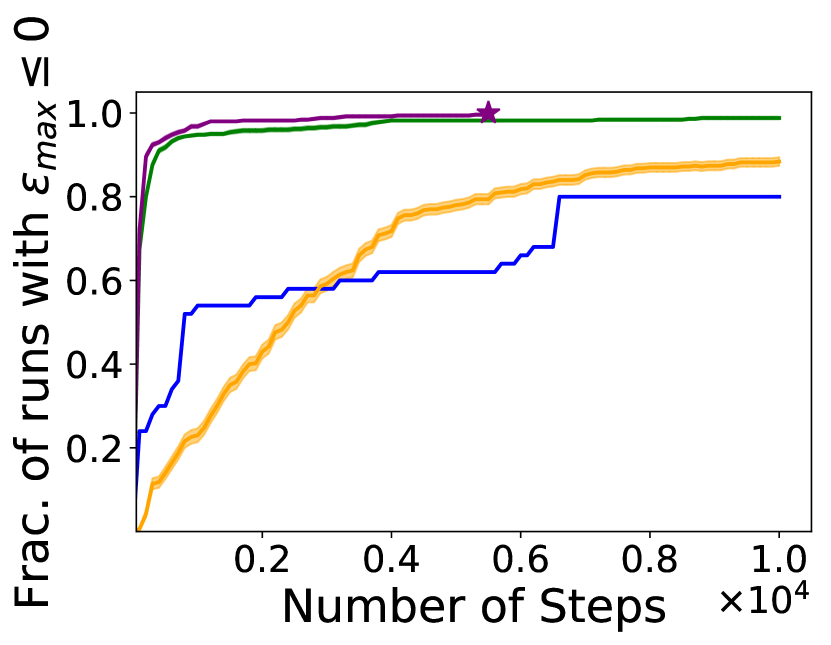
(a) TeamGoofspiel$\boldsymbol{(7)}$

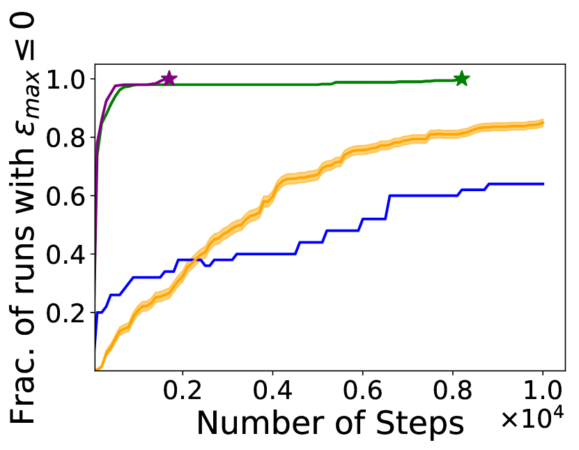
(b) TeamGoofspiel$\boldsymbol{(8)}$

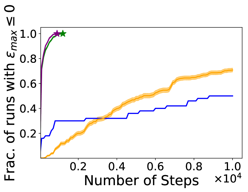
(c) TeamGoofspiel$\boldsymbol{(9)}$

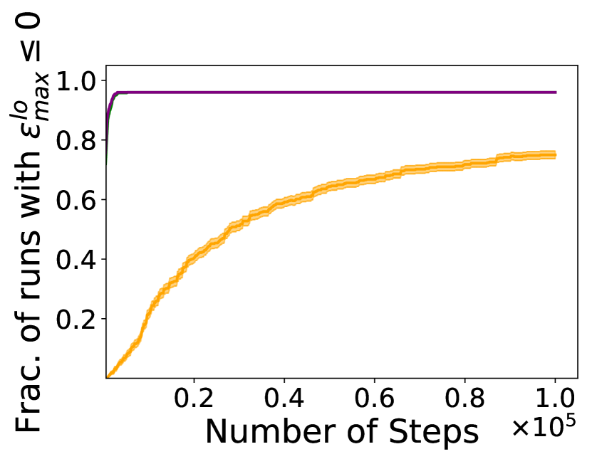
(d) TeamGoofspiel$\boldsymbol{(13)}$

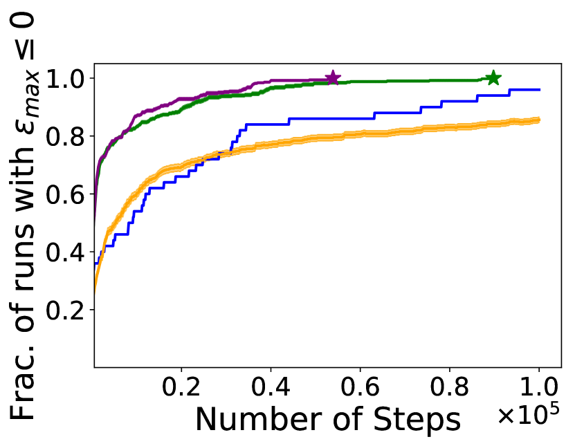
(e) Euchre$\boldsymbol{(8)}$

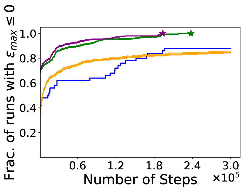
(f) Euchre$\boldsymbol{(9)}$

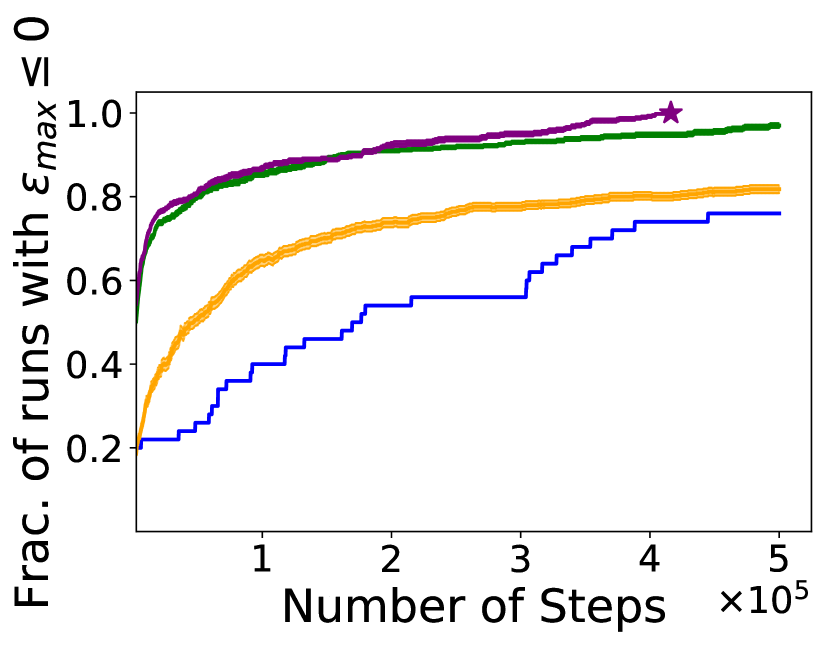
(g) Euchre$\boldsymbol{(10)}$

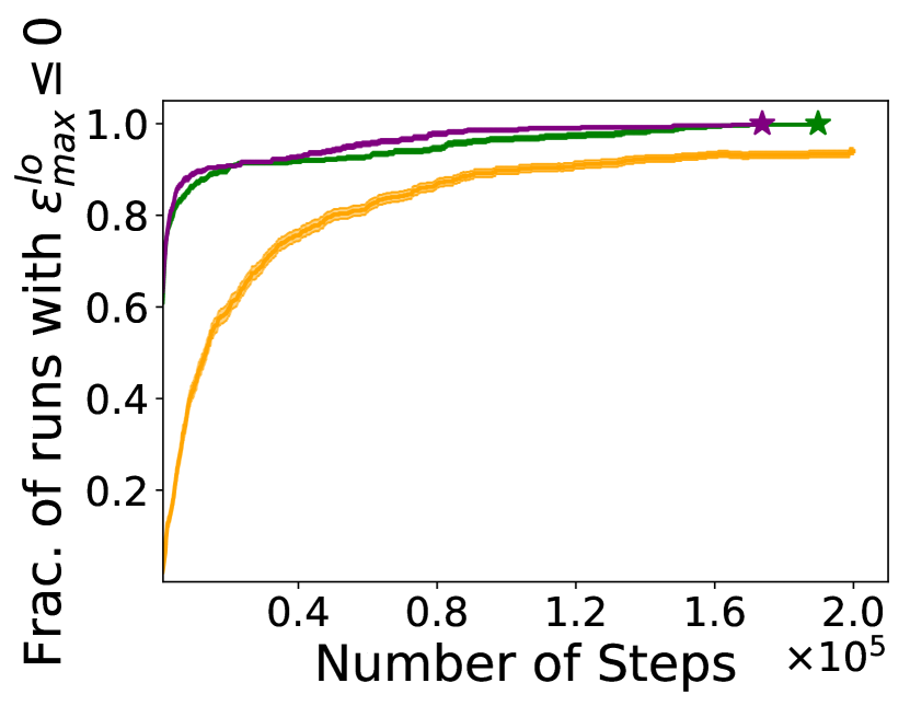
(h) Euchre$\boldsymbol{(12)}$

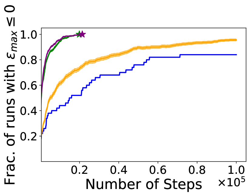
(i) Spades$\boldsymbol{(8)}$

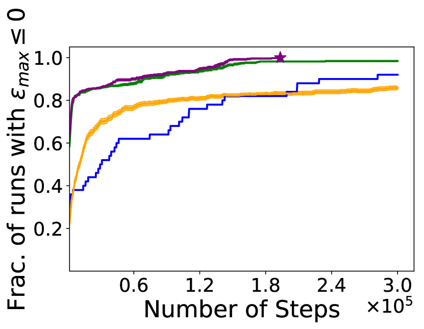
(j) Spades$\boldsymbol{(9)}$

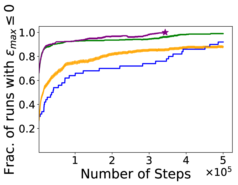
(k) Spades$\boldsymbol{(10)}$

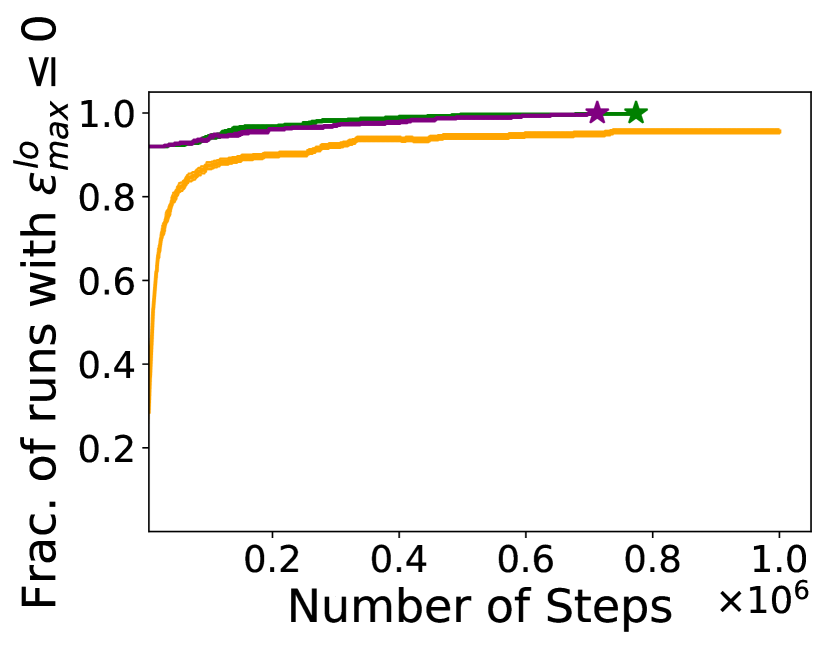
(l) Spades$\boldsymbol{(13)}$

Figure 3. Performance profiles on TeamGoofspiel, Euchre and Spades with known context. Shaded regions show standard deviation. We add a marker if at the current number of steps the fraction of runs with $\epsilon_{max}\leq 0$ or $\epsilon^{lo}_{max}\leq 0$ is $1$.

4.1. Environments and Policies

We consider three card games played by two teams of two players. The members of one team are referred to as opponents, and they are treated as part of the environment. The members of the other team are treated as agents, and they are denoted by $\text{Ag}0$ and $\text{Ag}1$. All players have the same (initial) information probability function, but different decision making policies.

TeamGoofspiel$\boldsymbol{(H)}$. The first game is a team variation of the card game Goofspiel, introduced in Triantafyllou et al. (2022). In this game, the initial hand of each player consists of $H$ cards. Typically, $H=13$. At each round, all players simultaneously discard one of their cards, after observing the round’s prize. The team which played the cards with highest total value collects the prize. After $H$ rounds, the team that accumulated the biggest prize wins the game. Agent $\text{Ag}0$ tries to always play the card whose value matches the round’s prize. If that card is not in $\text{Ag}0$’s hand, then it chooses a card based on which team is currently leading the game. Agent $\text{Ag}1$ chooses its card based on a comparison between the average value of its hand and the current round’s prize. Opponents follow the same stochastic policy which assigns a distribution on their hand based on the round’s prize and the current leading team. For more details on the rules of the game and the players’ policies see Triantafyllou et al. (2022).

Euchre$\boldsymbol{(H)}$. Second, we consider a turn-based trick-taking game. Each player is initially dealt $H$ cards from a standard deck, with $H$ typically being $5$. Next follows the calling phase, where the trump suit and the player who starts first are chosen. For simplicity, we omit this phase and make the aforementioned choices randomly. At each round, the first player discards one card. This card’s suit becomes the leading suit of the current round. The rest of the players (in clockwise order) have to follow the leading suit if possible, otherwise they are allowed to play any card from their hand. The winner of the round is determined by a game-specific card ranking which takes into account the trump and the lead suits. The player who won the previous round starts next. After $H$ rounds, the team with the most wins takes the game. The policies of agents $\text{Ag}0$ and $\text{Ag}1$ are based on the HIGH! policy Seelbinder (2012). The main idea of HIGH! is that “if your teammate leads the round then let them win”. We implement the policy of $\text{Ag}0$ to be slightly more aggressive than that of $\text{Ag}1$. Opponents’ policies follow the HIGH! principle only when they play last in a round, otherwise they follow a stochastic greedy policy which assigns higher probabilities to cards that have potential to win the round. For more information see Appendix D.

Spades$\boldsymbol{(H)}$. Our third card game is yet another trick-taking game which is similar to Euchre$(H)$, but with some key differences. For example, there is no calling phase and the trump suit is always spades. Before they start playing, the players must bid on the number of tricks they believe that they will have won after $H$ rounds, where typically $H=13$. Spades$(H)$ has a different card ranking than Euchre$(H)$, and also some additional rules on which cards are allowed to be discarded by the players at each time. At the end of the game, the score of each team is calculated based on the number of tricks it won and its initial bids. In case a team bid more than its won tricks, it receives a penalty based on a sandbagging rule. The players’ policies in Spades$(H)$ are very similar to the ones in Euchre$(H)$. For more information see Appendix E.

Note that all three games are standard benchmarks for AI research Hennes et al. (2020); Kaur and Haar (2005); Cowling et al. (2014); Baier et al. (2018), and have also received extensive mathematical analysis Ross (1971); Rhoads and Bartholdi (2012); Grimes and Dror (2013); Wright (2001); Cohensius et al. (2019). Moreover, Goofspiel and Euchre are parts of a well known framework for RL in games Lanctot et al. (2019).

4.2. Experimental Setup

(a) TeamGoofspiel$\boldsymbol{(9)}$ Unc.

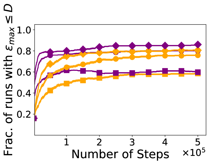
(b) Euchre$\boldsymbol{(10)}$ Unc.

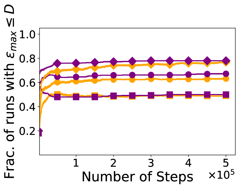
(c) Spades$\boldsymbol{(10)}$ Unc.

Figure 4. Performance profiles on TeamGoofspiel$\boldsymbol{(9)}$, Euchre$\boldsymbol{(10)}$ and Spades$\boldsymbol{(10)}$ with unknown context. Shaded regions show standard deviation and number of steps are per sample. The full set of plots can be found in Appendix H.

We evaluate the efficacy of several search algorithms on estimating a responsibility assignment under a computational budget. Computational budget in our experiments is defined as the total number of environment steps that an algorithm is allowed to take.

Baselines. Apart from RA-MCTS we also implement RANDOM, which repeatedly samples a set of interventions and checks whether it constitutes a candidate actual cause-witness pair or not. When computational budget is reached, RANDOM determines the agents’ degrees of responsibility based on the found solutions. Other baselines are BF-DT and BF-ST, which perform a brute force search over all possible sets of interventions. BF-DT is the algorithm of choice in Triantafyllou et al. (2022), and it utilizes the standard decision (game) tree. On the other hand, BF-ST utilizes the search tree from Section 3.1.

Performance profiles. We generate multiple configurations of our environments by changing parameter $H$. For each of these configurations, our methods are evaluated on $50$ different trajectories, in which the agents fail to win the opponents. For each such trajectory, we perform $10$ independent runs of each method. Following Agarwal et al. (2021), we report performance profiles based on run-score distributions, and show for each method the fraction of runs in which it performs better than a certain threshold $D$. We measure the performance of a method in terms of its accuracy w.r.t. some target responsibility assignment. More specifically, when it is computationally feasible to find the exact responsibility assignment, we report the maximum absolute difference $\epsilon_{max}\in[0,1]$. For instance, if for some trajectory the agents’ degrees of responsibility according to a method are $0.25$ and $0.75$, but the exact degrees are $0.33$ and $1$, then $\epsilon_{max}=0.25$. If instead of the exact values, we can only compute lower bounds of the agents’ responsibilities, we report the maximum absolute lower difference $\epsilon^{lo}_{max}\in[0,1]$. Going back to our previous example, if the known lower bounds are $0.33$ and $0.5$, then $\epsilon^{lo}_{max}=0.08$.

For Euchre$(H)$ and Spades$(H)$, we are able compute the exact responsibility assignments for values of $H$ up to $10$. For TeamGoofspiel$(H)$, the upper limit is $9$. In order to evaluate our methods on environments with larger $H$, we follow a procedure, described in Appendix F, and generate trajectories for which we can retrieve non-trivial lower bounds of the agents’ degrees of responsibility.

4.3. Results

4.3.1. Results with Known Context

Plots 3(a)-3(l) display performance profiles for the implemented methods and for different computational budgets. Note that threshold $D$ in these experiments is set to $0$. This means that a method performs better than $D$ iff it manages to find the exact responsibility assignment.

We observe that RA-MCTS almost always converges to the optimal solution, i.e., achieves $\epsilon_{max}=0$ or $\epsilon^{lo}_{max}=0$, under a reasonable computational budget. The only exception is TeamGoofspiel$(13)$, for which it converges for $96\%$ of the runs. To better understand how budget efficient RA-MCTS is, consider configurations Euchre$(10)$ and Spades$(10)$. By looking at Plots 3(g) and 3(k), we observe that RA-MCTS needs at most $4.2\cdot 10^{5}$ and $3.5\cdot 10^{5}$ environment steps in order to converge to the exact responsibility assignment in these two configurations. In comparison, performing an exhaustive search, i.e., fully executing BF-DT or BF-ST, on one trajectory of Euchre$(10)$ and one of Spades$(10)$ can take up to more than $10\cdot 10^{9}$ and $6.2\cdot 10^{9}$ steps, respectively. It is also worth noting that RA-MCTS achieves $\epsilon_{max}=0$ for more than $90\%$ of the runs, in the above mentioned configurations, within at most $2\cdot 10^{5}$ and $0.5\cdot 10^{5}$ steps.

By comparing RA-MCTS to RANDOM in Plots 3(a)-3(l), we can see that the former always stochastically dominates the latter Levy (1992). As part of our ablation study, we also compare RA-MCTS to BF-ST. In Plots 3(a)-3(c) and 3(e)-3(k), RA-MCTS stochastically dominates BF-ST. In Plot 3(c), performance profiles of the two methods are almost identical, while in Plot 3(l), BF-ST outperforms RA-MCTS only for a small number of steps. Moreover, it can be seen that almost always the maximum number of environment steps that RA-MCTS might need in order to find the exact responsibility assignment, is considerably less than that of BF-ST. For instance, in Plot 3(b) RA-MCTS needs almost $5$ times fewer environment steps compared to BF-ST, while in Plots 3(a), 3(e), 3(j), 3(k) we witness a drop of at least $30\%$. These results show that components from Sections 3.2 and 3.3 are important for RA-MCTS. In Appendix G, we include a similar ablation study, where we compare RA-MCTS to the BF-ST method enhanced with the pruning technique described in Section 3.2.

Finally, Plots 3(a)-3(l) showcase that BF-ST stochastically dominates BF-DT. This result demonstrates that a brute force algorithm that uses the structure of the tree we propose in Section 3.2 converges faster to the exact solution than a brute force algorithm that uses the standard decision tree of the underlying Dec-POMDP.

4.3.2. Results with Unknown Context

In this section, we present the results of our experiments under context uncertainty, where we make use of the sampling procedure introduced in Section 3.4, with total number of samples $M=10$. Each sample corresponds to a context generated by posterior inference. Plots 4(a)-4(c) display performance profiles for methods RA-MCTS and RANDOM for different computational budgets and for different values of threshold $D$. First, we observe that almost always RA-MCTS stochastically dominates RANDOM. Moreover, all plots show that RA-MCTS achieves $\epsilon_{max}=0.25$ in more than $75\%$ of the runs, within at most $0.5\cdot 10^{5}$ steps per sample, or $5\cdot 10^{5}$ steps in total. Finally, we can also see that our method performs the best for TeamGoofspiel$(9)$, where it achieves $\epsilon_{max}=0.15$ in $86\%$ of the runs.

Our results give prominence to an inherent problem of responsibility attribution under context uncertainty. We observe that even for a number of steps that suffices for RA-MCTS to find the exact agents’ degrees of responsibility for most of the sampled trajectories, the responsibility assignments for many of the actual trajectories are not fully found. We conclude then that even under unbounded computational budget if the posterior distribution of the underlying context of a trajectory is not informative enough, then failing to exactly estimate the agents’ degrees of responsibility for that trajectory is unavoidable. We believe however that one potential way to alleviate this issue is by designing responsibility attribution mechanisms that incorporate domain knowledge, which could balance the non-informativeness of the posterior distribution.

5. Conclusion

We initiate the study of developing efficient algorithmic approaches for responsibility attribution in Dec-POMDPs. To that end, we propose and experimentally evaluate RA-MCTS, an MCTS type of method which efficiently approximates responsibility assignments. Looking forward, we plan to apply and test the efficiency of RA-MCTS on a real-world domain. Extending our approach to continuous models is another research direction that we deem particularly interesting.

Appendix A List of Appendices

In this section, we provide a brief description of the content provided in the appendices of the paper.

• Appendix B provides an extended discussion on the application scenario of autonomous traffic light control.

• Appendix C provides additional information on Gumbel-Max SCMs.

• Appendix D provides additional details on the players’ policies in the Euchre environment from Section 4.1.

• Appendix E provides additional details on the players’ policies in the Spades environment from Section 4.1.

• Appendix F provides the details of our experimental setup for large size environments.

• Appendix G includes the results of an additional ablation study on RA-MCTS.

• Appendix H includes the remaining plots from Section 4.3.2.

Appendix B Extended Discussion on Possible Application Scenario

In this section we discuss a possible application scenario for our proposed algorithmic framework. We consider autonomous traffic light control (ATLC) systems Arel et al. (2010). Typically, in ATLC each agent controls one road intersection. At every time-step, the agent observes some local information, and depending on the system’s exact implementation it might as well receive messages from other agents. Based on this information, the agent then decides on how to schedule the traffic lights of the intersection it controls. A common failure example in ATLC includes a driver waiting in some intersection for more than an “acceptable” time period. In systems as complex as ATLC, however, it is hard to identify who might have caused such a failure. This is due to the temporal dependencies between the agents’ decisions. The system designers might want to determine, for instance, whether the agent who controls the intersection where the driver had to wait made a mistake? Or was the failure (partly) caused by mistakes made by other agents in previous time-steps? This is where our algorithmic framework for attributing responsibility can prove useful. In a scenario like this, our method can efficiently approximate the degree to which each agent contributed to the system’s failure.

From a technical perspective, we mention that our search method is generic and can be technically applied to any setting modeled as a finite and discrete Dec-POMDP. There are recent works that model ATLC as Dec-POMDPs Jiang et al. (2022).

Appendix C Gumbel-Max SCMs

In this section, we show how to implement Gumbel-Max SCMs in the Dec-POMDP SCM setting. Furthermore, we provide intuition behind a desirable property they satisfy. For more details, we refer the interested reader to Oberst and Sontag (2019).

Under the Gumbel-Max model, the structural equations of Eq. (2.2) become:

$$S_{t}=\operatorname*{arg\,max}_{s\in\mathcal{S}}\{\log P(S_{t-1},A_{t-1},S_{t}=s)+U_{S_{t}}\}$$

$$O_{t}=\operatorname*{arg\,max}_{o\in\mathcal{O}}\{\log\Omega(S_{t},O_{t}=o)+U_{O_{t}}\}$$

$$I_{i,t}=\operatorname*{arg\,max}_{\imath_{i}\in\mathcal{I}_{i}}\{\log Z_{i}(I_{i,t-1},A_{i,t-1},O_{t},I_{i,t}=\imath_{i})+U_{I_{i,t}}\}$$

$$A_{i,t}=\operatorname*{arg\,max}_{a_{i}\in\mathcal{A}_{i}}\{\log\pi_{i}(A_{i,t}=a_{i}|I_{i,t})+U_{A_{i,t}}\}$$

where $U_{S_{t}}$, $U_{O_{t}}$, $U_{I_{i,t}}$ and $U_{A_{i,t}}\sim$ Gumbel$(0,1)$.

It has been shown that the class of Gumbel-Max SCMs satisfies a desirable property for categorical SCMs, namely the counterfactual stability property. This property is considered important because it excludes a specific type of non-intuitive counterfactual outcomes. What follows, is an example taken from Triantafyllou et al. (2022) which aims to provide the main intuition behind this property. Consider the observed trajectory $\tau=\{(s_{t},a_{t})\}_{t=0}^{T-1}$, and the counterfactual scenario in which agents $\{1,...,n\}$ take the joint action $a^{\prime}$ at time-step $t$, instead of $a_{t}$. The counterfactual stability property ensures that under this counterfactual scenario, it is impossible that at time-step $t+1$ the process would transition to a state $s^{\prime}$ different than the observed state, i.e., $s_{t+1}$, if the following condition holds

$$\frac{P(S_{t}=s,A_{t}=a^{\prime},S_{t+1}=s_{t+1})}{P(S_{t}=s,A_{t}=a_{t},S_{t+1}=s_{t+1})}\geq\frac{P(S_{t}=s,A_{t}=a^{\prime},S_{t+1}=s^{\prime})}{P(S_{t}=s,A_{t}=a_{t},S_{t+1}=s^{\prime})}.$$

In other words, in order for the state at time-step $t+1$ to change under a counterfactual scenario, the relative likelihood of an alternative state $s^{\prime}$ must have increased compared to that of $s_{t+1}$.

Appendix D Additional Details on Euchre

In this section, we present the agents’ and opponents’ for the card game Euchre, which was described in Section 4.1.

Information states of all players include the trump suit, the leading suit of the current round, their hand and the current trick.

Agents have deterministic policies which differ from each other’s. If they are the first to play on a round: $\text{Ag}0$ plays the lowest ranked card on its hand, while $\text{Ag}1$ plays its highest ranked card that (if possible) is not from the trump suit. When playing second or third on a round: both agents play their worst valid card if their teammate is leading the round or if they do not have any winning card, otherwise $\text{Ag}0$ plays the worst of its winning cards and $\text{Ag}1$ plays its best such card. When playing last: they both play their lowest ranked winning card, and if they do not have a winning card then they just play their lowest ranked valid card.

Opponents share the same stochastic policy. If they are the first to play on a round: then they pick a card from their hand uniformly at random. When playing second or third on a round: they play with $0.8$ probability a winning card or their lowest ranked valid card in case they do not have winning cards. When playing last: they play with $0.8$ probability a winning card or their lowest ranked valid card in case they do not have winning cards or their teammate is leading the round.

Appendix E Additional Details on Spades

In this section, we present the agents’ and opponents’ policies for the card game Spades, which was described in Section 4.1. Each player’s policy is divided into a bidding policy and playing policy. The former is activated during the bidding phase of the game, while the latter in the playing phase. The playing policies of the players are almost identical to the ones the players follow in Euchre, and can be found in Appendix D. Regarding their bidding policies, all players adhere to the following mechanism which is based on the player’s initial hand. The player starts with bid $0$, and increases it by $1$ for every for every King and Ace they have, and also if they have the Jack or Queen of spades. They also add to their bid the total number of cards they have with suit of spades and value below Jack, divided by $\frac{H}{3}$, where $H$ is the initial size of their hand.

Appendix F Lower Bounds of Responsibility Degrees for Large Environments

In this section, we describe the procedure that we follow to generate a trajectory for which we can compute lower bounds of the agents’ degrees of responsibility, when the size of the environment is too large to compute them exactly (see Section 4.2). Note that the same procedure is used for all the environments.

First, we randomly pick $5$ action variables for each agent. For each one of those variables, we “poison” the agent’s policy, such that zero probability is assigned to the action that the agent’s non-poisoned (deterministic) policy would have normally taken, and all other valid actions are assigned equal probabilities. Next, we sample a trajectory in which the agents win by using their non-poisoned policies. We then fix the context that was used to generate the previous trajectory, and simulate the agents’ poisoned policies in the environment. We repeat the last two steps, until the outcome of the latter trajectory signifies a loss for the agents. In order to compute lower bounds for the agents’ degrees of responsibility on the failed trajectory, all we have to do is execute a brute force method (e.g., BF-DT) restricted to the action variables that were poisoned.

Note that there can be actual cause-witness pairs with variables that are not checked by the search, and hence why the above mentioned procedure provides lower bounds of the responsibilities and not their exact values. The pool of action variables the brute force is restricted to however, is promising for finding actual cause-witness pairs, and that is why the lower bounds this mechanism computes are not trivial.

Appendix G Additional Ablation Study

(a) TeamGoofspiel$\boldsymbol{(7)}$

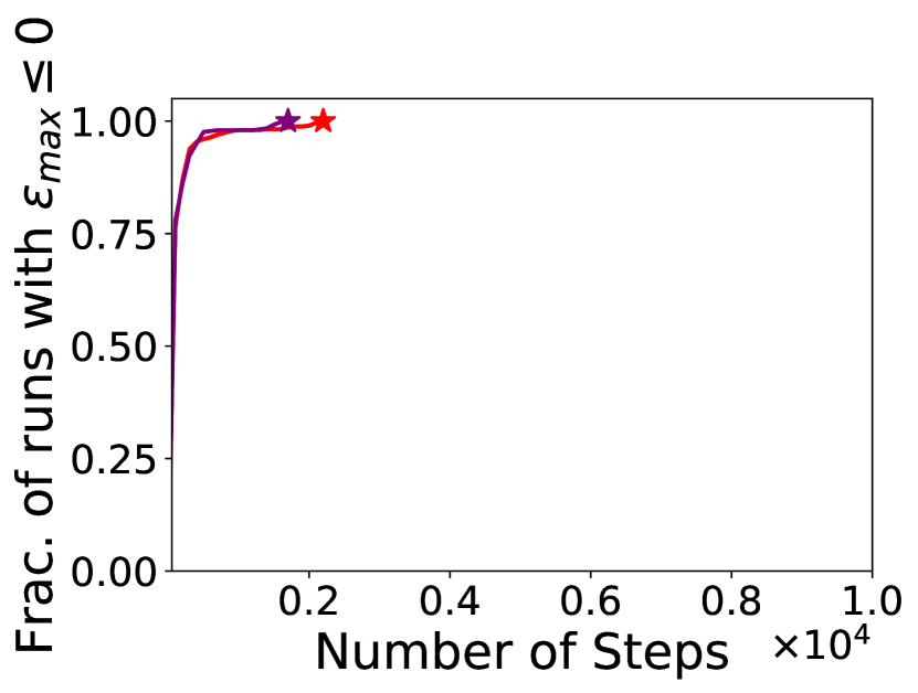
(b) TeamGoofspiel$\boldsymbol{(8)}$

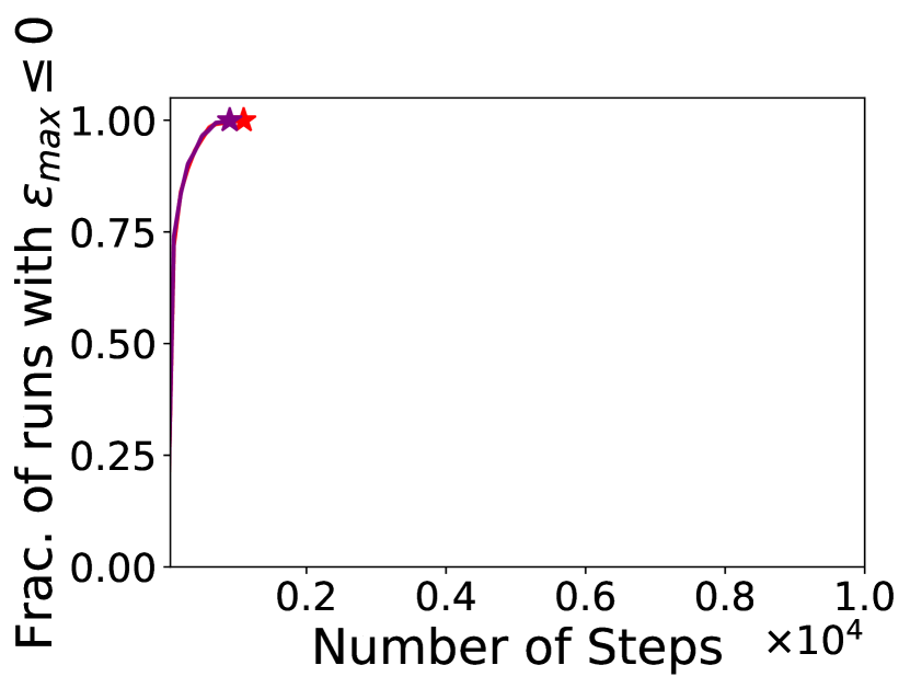
(c) TeamGoofspiel$\boldsymbol{(9)}$

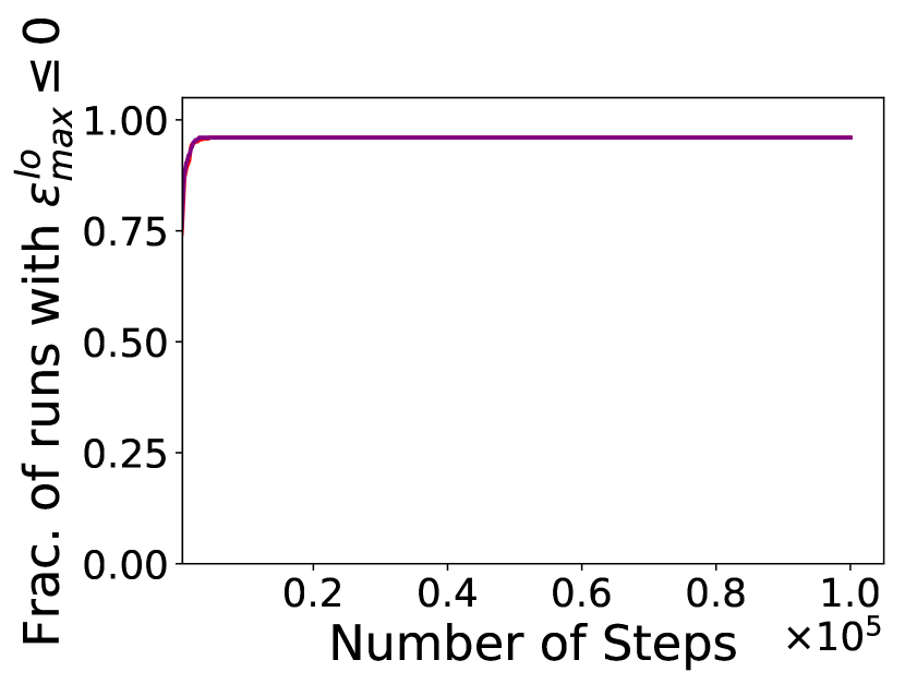
(d) TeamGoofspiel$\boldsymbol{(13)}$

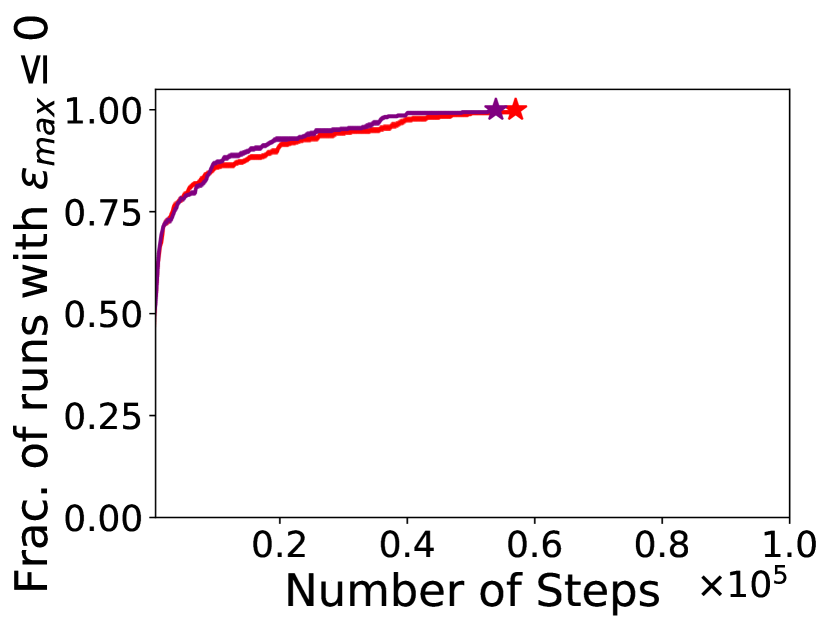
(e) Euchre$\boldsymbol{(8)}$

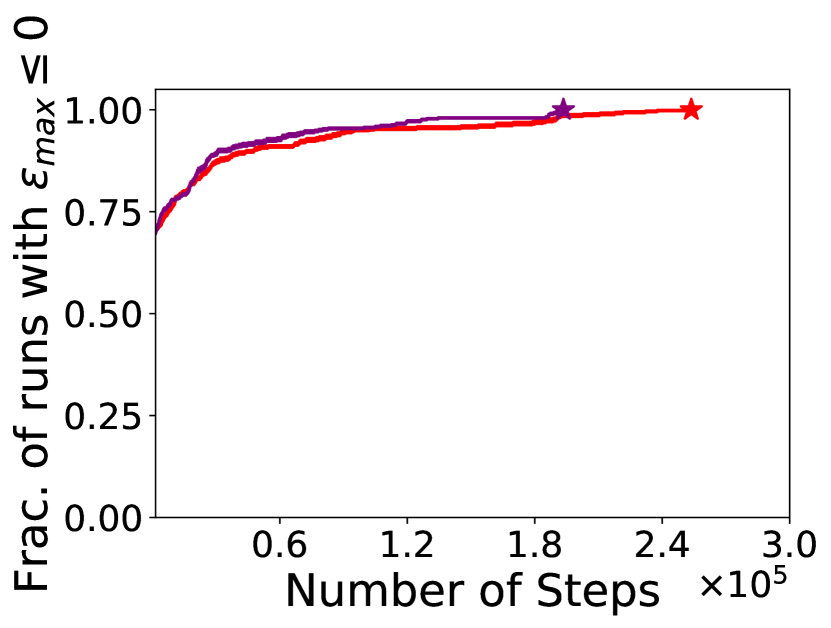
(f) Euchre$\boldsymbol{(9)}$

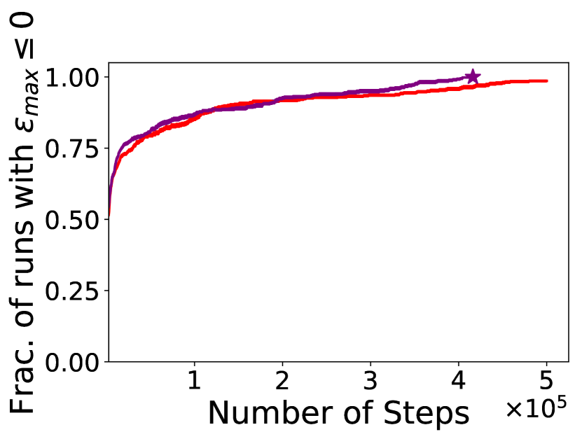
(g) Euchre$\boldsymbol{(10)}$

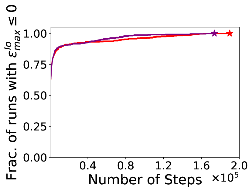
(h) Euchre$\boldsymbol{(12)}$

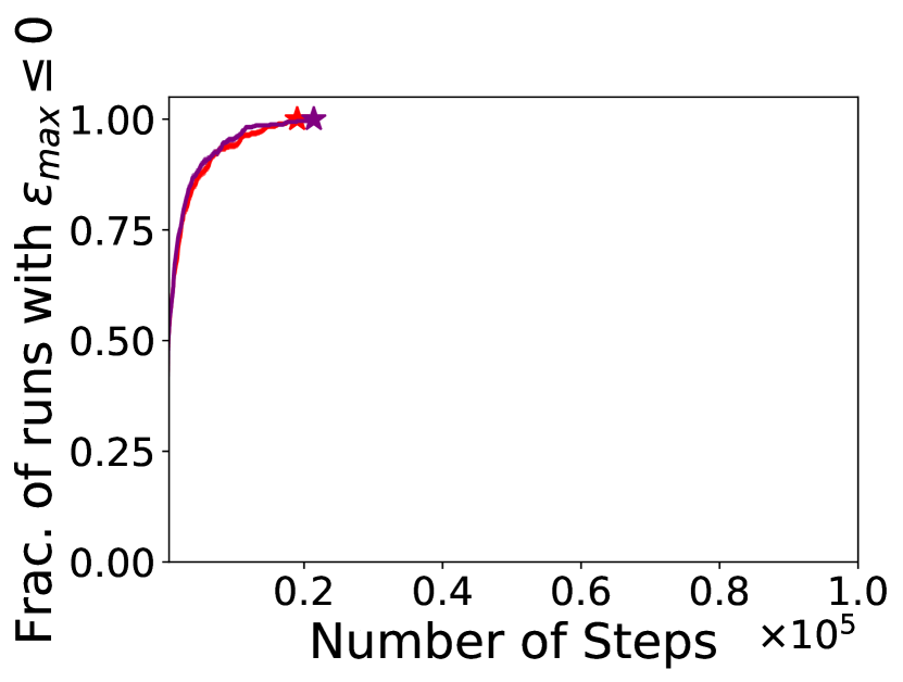
(i) Spades$\boldsymbol{(8)}$

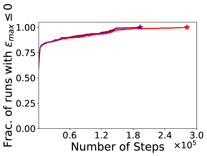
(j) Spades$\boldsymbol{(9)}$

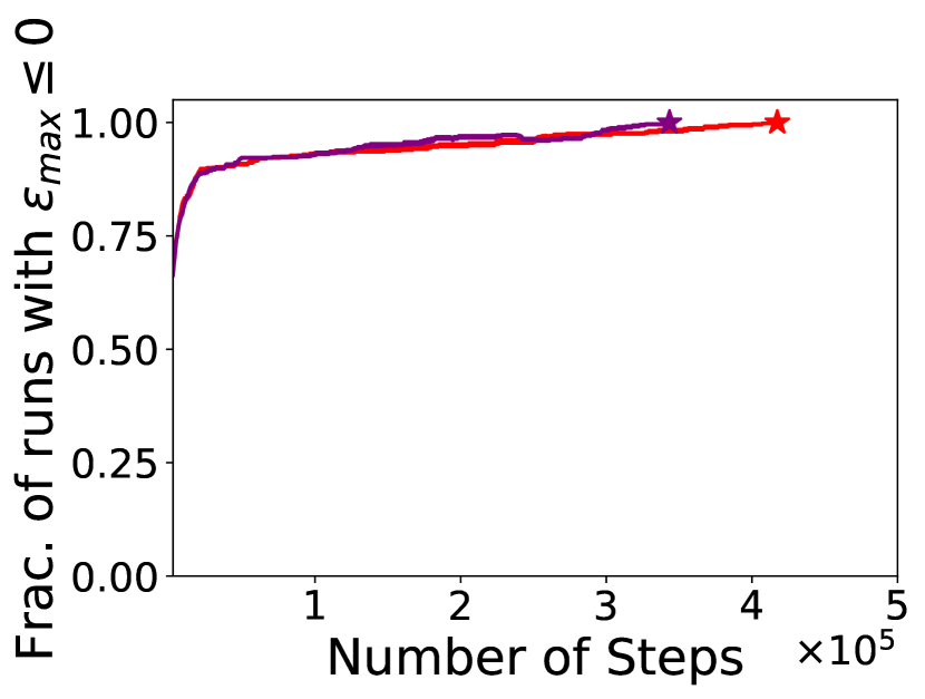
(k) Spades$\boldsymbol{(10)}$

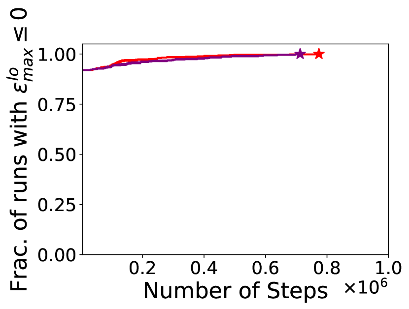
(l) Spades$\boldsymbol{(13)}$

Figure 5. Performance profiles on TeamGoofspiel, Euchre and Spades with known context. Shaded regions show standard deviation. We add a marker if at the current number of steps the fraction of runs with $\epsilon_{max}\leq 0$ or $\epsilon^{lo}_{max}\leq 0$ is $1$. Plots in this figure are part of our ablation study, and they are used to compare RA-MCTS to BF-ST-PRUN.

As part of our ablation study, we compare RA-MCTS to method BF-ST-PRUN, which is essentially the method BF-ST from Section 4.2 enhanced with the pruning technique described in Section 3.2. By looking at the plots in Fig. 5, we conclude that the effects that can be seen when comparing RA-MCTS and BF-ST-PRUN, are similar albeit less prominent to those for RA-MCTS and BF-ST. These results showcase that components from Section 3.3 are important for RA-MCTS.

Appendix H Additional Results with Unknown Context

Fig. 6 contains the full set of plots for results with unknown context (Section 4.3.2).

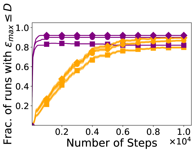
(a) TeamGoofspiel$\boldsymbol{(7)}$ Unc.

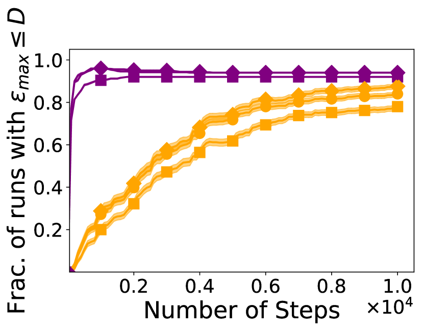
(b) TeamGoofspiel$\boldsymbol{(8)}$ Unc.

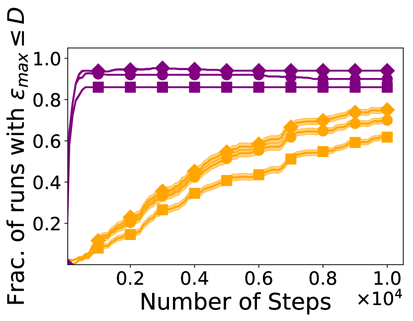
(c) TeamGoofspiel$\boldsymbol{(9)}$ Unc.

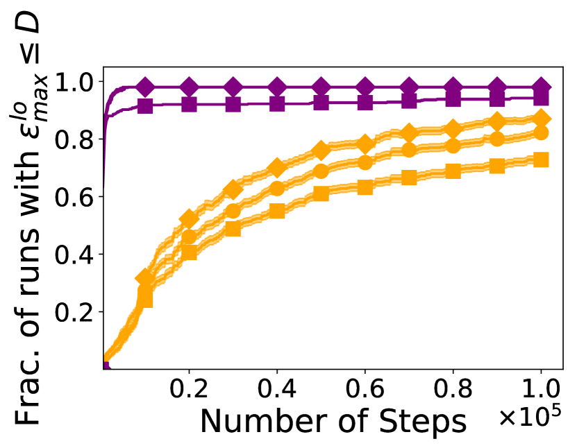
(d) TeamGoofspiel$\boldsymbol{(13)}$ Unc.

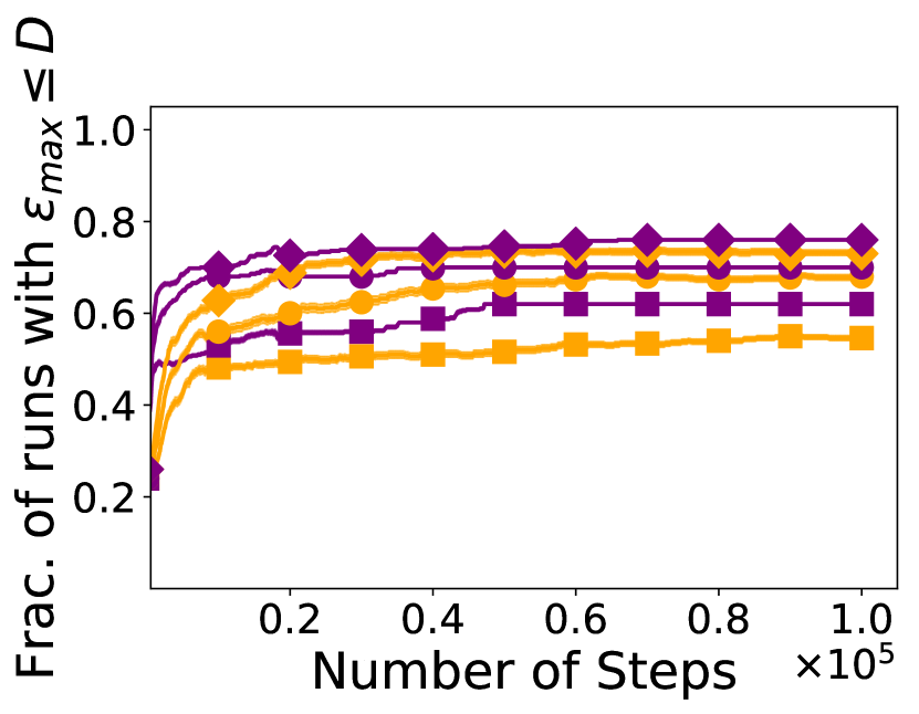
(e) Euchre$\boldsymbol{(8)}$ Unc.

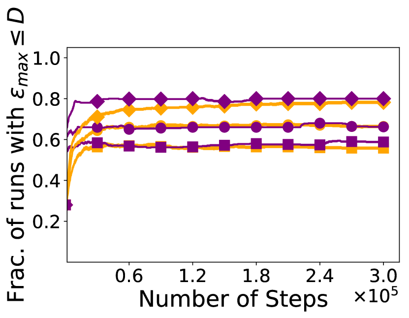
(f) Euchre$\boldsymbol{(9)}$ Unc.

(g) Euchre$\boldsymbol{(10)}$ Unc.

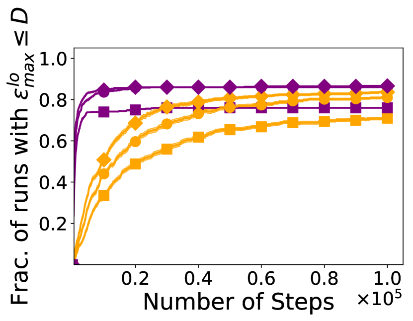
(h) Euchre$\boldsymbol{(12)}$ Unc.

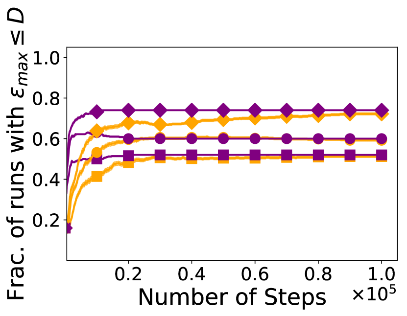
(i) Spades$\boldsymbol{(8)}$ Unc.

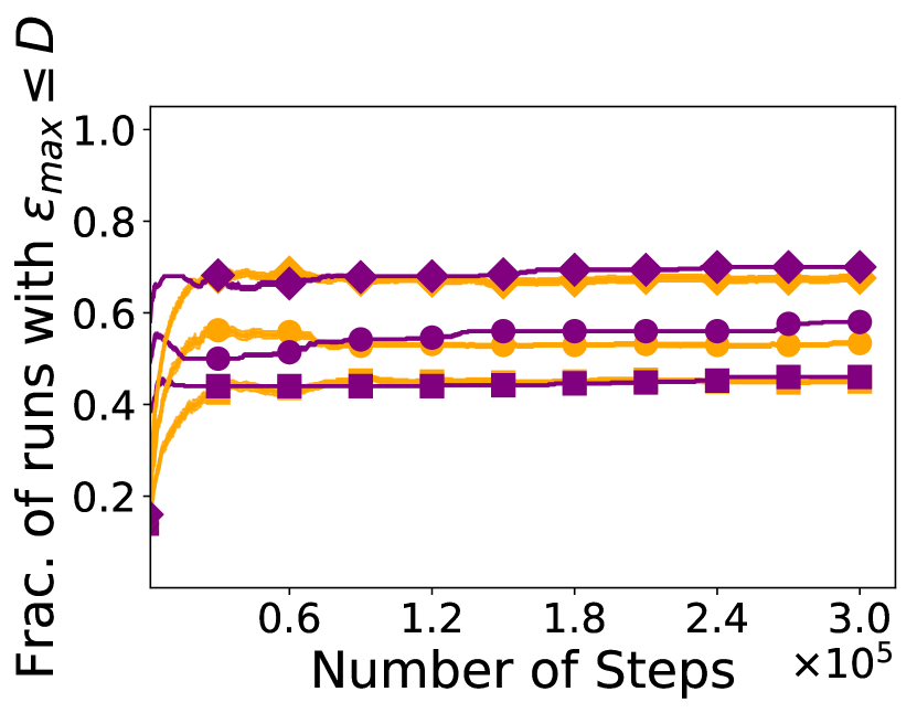
(j) Spades$\boldsymbol{(9)}$ Unc.

(k) Spades$\boldsymbol{(10)}$ Unc.

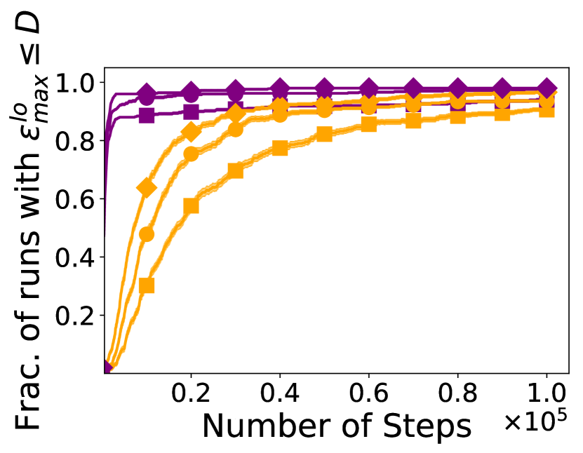
(l) Spades$\boldsymbol{(13)}$ Unc.

Figure 6. Performance profiles on TeamGoofspiel, Euchre and Spades with unknown context. Shaded regions show standard deviation. Each curve corresponds to a pair of method and threshold $D$.

References

- (1)
- Agarwal et al. (2021) Rishabh Agarwal, Max Schwarzer, Pablo Samuel Castro, Aaron C. Courville, and Marc Bellemare. 2021. Deep reinforcement learning at the edge of the statistical precipice. Advances in Neural Information Processing Systems 34 (2021), 29304–29320.
- Ahmed et al. (2020) Umair Ahmed, Maria Christakis, Aleksandr Efremov, Nigel Fernandez, Ahana Ghosh, Abhik Roychoudhury, and Adish Singla. 2020. Synthesizing tasks for block-based programming. Advances in Neural Information Processing Systems 33 (2020), 22349–22360.
- Alechina et al. (2020) Natasha Alechina, Joseph Y. Halpern, and Brian Logan. 2020. Causality, responsibility and blame in team plans. arXiv preprint arXiv:2005.10297 (2020).
- Aleksandrowicz et al. (2017) Gadi Aleksandrowicz, Hana Chockler, Joseph Y. Halpern, and Alexander Ivrii. 2017. The computational complexity of structure-based causality. Journal of Artificial Intelligence Research 58 (2017), 431–451.
- Arel et al. (2010) Itamar Arel, Cong Liu, Tom Urbanik, and Airton G. Kohls. 2010. Reinforcement learning-based multi-agent system for network traffic signal control. IET Intelligent Transport Systems 4, 2 (2010), 128–135.
- Auer et al. (2002) Peter Auer, Nicolo Cesa-Bianchi, and Paul Fischer. 2002. Finite-time analysis of the multiarmed bandit problem. Machine learning 47, 2 (2002), 235–256.
- Baier et al. (2021a) Christel Baier, Florian Funke, and Rupak Majumdar. 2021a. A game-theoretic account of responsibility allocation. arXiv preprint arXiv:2105.09129 (2021).
- Baier et al. (2021b) Christel Baier, Florian Funke, and Rupak Majumdar. 2021b. Responsibility attribution in parameterized Markovian models. In Proc. of the 35th AAAI Conference on Artificial Intelligence (AAAI). 11734–11743.
- Baier et al. (2018) Hendrik Baier, Adam Sattaur, Edward J. Powley, Sam Devlin, Jeff Rollason, and Peter I. Cowling. 2018. Emulating human play in a leading mobile card game. IEEE Transactions on Games 11, 4 (2018), 386–395.
- Bernstein et al. (2002) Daniel S. Bernstein, Robert Givan, Neil Immerman, and Shlomo Zilberstein. 2002. The complexity of decentralized control of Markov decision processes. Mathematics of Operations Research 27, 4 (2002), 819–840.
- Bjornsson and Finnsson (2009) Yngvi Bjornsson and Hilmar Finnsson. 2009. Cadiaplayer: A simulation-based general game player. IEEE Transactions on Computational Intelligence and AI in Games 1, 1 (2009), 4–15.
- Browne et al. (2012) Cameron B. Browne, Edward Powley, Daniel Whitehouse, Simon M. Lucas, Peter I. Cowling, Philipp Rohlfshagen, Stephen Tavener, Diego Perez, Spyridon Samothrakis, and Simon Colton. 2012. A survey of monte carlo tree search methods. IEEE Transactions on Computational Intelligence and AI in games 4, 1 (2012), 1–43.
- Buesing et al. (2018) Lars Buesing, Theophane Weber, Yori Zwols, Sebastien Racaniere, Arthur Guez, Jean-Baptiste Lespiau, and Nicolas Heess. 2018. Woulda, coulda, shoulda: Counterfactually-guided policy search. arXiv preprint arXiv:1811.06272 (2018).
- Chaslot et al. (2008) Guillaume Chaslot, Sander Bakkes, Istvan Szita, and Pieter Spronck. 2008. Monte-carlo tree search: A new framework for game AI. In Proceedings of the AAAI Conference on Artificial Intelligence and Interactive Digital Entertainment, Vol. 4. 216–217.
- Chockler et al. (2008a) Hana Chockler, Orna Grumberg, and Avi Yadgar. 2008a. Efficient automatic STE refinement using responsibility. In International Conference on Tools and Algorithms for the Construction and Analysis of Systems. Springer, 233–248.
- Chockler and Halpern (2004) Hana Chockler and Joseph Y. Halpern. 2004. Responsibility and blame: A structural-model approach. Journal of Artificial Intelligence Research 22 (2004), 93–115.
- Chockler et al. (2008b) Hana Chockler, Joseph Y. Halpern, and Orna Kupferman. 2008b. What causes a system to satisfy a specification? ACM Transactions on Computational Logic (TOCL) 9, 3 (2008), 1–26.
- Cohensius et al. (2019) Gal Cohensius, Reshef Meir, Nadav Oved, and Roni Stern. 2019. Bidding in spades. arXiv preprint arXiv:1912.11323 (2019).
- Coulom (2006) Rémi Coulom. 2006. Efficient selectivity and backup operators in Monte-Carlo tree search. In International Conference on Computers and Games. Springer, 72–83.
- Cowling et al. (2014) Peter I. Cowling, Sam Devlin, Edward J Powley, Daniel Whitehouse, and Jeff Rollason. 2014. Player preference and style in a leading mobile card game. IEEE Transactions on Computational Intelligence and AI in Games 7, 3 (2014), 233–242.
- Drugan and Nowe (2013) Madalina M. Drugan and Ann Nowe. 2013. Designing multi-objective multi-armed bandits algorithms: A study. In The 2013 International Joint Conference on Neural Networks (IJCNN). IEEE, 1–8.
- Eiter and Lukasiewicz (2002) Thomas Eiter and Thomas Lukasiewicz. 2002. Complexity results for structure-based causality. Artificial Intelligence 142, 1 (2002), 53–89.
- Friedenberg and Halpern (2019) Meir Friedenberg and Joseph Y. Halpern. 2019. Blameworthiness in multi-agent settings. In Proceedings of the AAAI Conference on Artificial Intelligence, Vol. 33. 525–532.
- Grimes and Dror (2013) Mark Grimes and Moshe Dror. 2013. Observations on strategies for Goofspiel. In 2013 IEEE Conference on Computational Inteligence in Games (CIG). 1–2.
- Halpern (2015) Joseph Y. Halpern. 2015. A modification of the Halpern-Pearl definition of causality. In Twenty-Fourth International Joint Conference on Artificial Intelligence.
- Halpern (2016) Joseph Y. Halpern. 2016. Actual causality. MiT Press.
- Halpern and Hitchcock (2011) Joseph Y. Halpern and Christopher Hitchcock. 2011. Actual causation and the art of modeling. arXiv preprint arXiv:1106.2652 (2011).
- Halpern and Kleiman-Weiner (2018) Joseph Y. Halpern and Max Kleiman-Weiner. 2018. Towards formal definitions of blameworthiness, intention, and moral responsibility. In Proceedings of the AAAI Conference on Artificial Intelligence, Vol. 32.
- Halpern and Pearl (2005) Joseph Y. Halpern and Judea Pearl. 2005. Causes and explanations: A structural-model approach. Part I: Causes. British Journal for the Philosophy of Science 56, 4 (2005).
- Hennes et al. (2020) Daniel Hennes, Dustin Morrill, Shayegan Omidshafiei, Rémi Munos, Julien Perolat, Marc Lanctot, Audrunas Gruslys, Jean-Baptiste Lespiau, Paavo Parmas, Edgar Duéñez-Guzmán, et al. 2020. Neural replicator dynamics: Multiagent learning via hedging policy gradients. In Proceedings of the 19th International Conference on Autonomous Agents and MultiAgent Systems. 492–501.
- Hiddleston (2005) Eric Hiddleston. 2005. Causal powers. The British Journal for the Philosophy of Science 56, 1 (2005), 27–59.
- Ibrahim et al. (2019) Amjad Ibrahim, Simon Rehwald, and Alexander Pretschner. 2019. Efficient checking of actual causality with sat solving. Engineering Secure and Dependable Software Systems 53 (2019), 241.
- Jiang et al. (2022) Qize Jiang, Minhao Qin, Shengmin Shi, Weiwei Sun, and Baihua Zheng. 2022. Multi-agent reinforcement learning for traffic signal control through universal communication method. arXiv preprint arXiv:2204.12190 (2022).
- Kaur and Haar (2005) D Kaur and J Haar. 2005. Fuzzy logic based Euchre game design on palm PDA. In NAFIPS 2005-2005 Annual Meeting of the North American Fuzzy Information Processing Society. IEEE, 693–699.
- Kocsis and Szepesvári (2006) Levente Kocsis and Csaba Szepesvári. 2006. Bandit based monte-carlo planning. In European conference on machine learning. Springer, 282–293.
- Lanctot et al. (2019) Marc Lanctot, Edward Lockhart, Jean-Baptiste Lespiau, Vinicius Zambaldi, Satyaki Upadhyay, Julien Pérolat, Sriram Srinivasan, Finbarr Timbers, Karl Tuyls, Shayegan Omidshafiei, et al. 2019. OpenSpiel: A framework for reinforcement learning in games. arXiv preprint arXiv:1908.09453 (2019).
- Levy (1992) Haim Levy. 1992. Stochastic dominance and expected utility: Survey and analysis. Management Science 38, 4 (1992), 555–593.
- Lorberbom et al. (2021) Guy Lorberbom, Daniel D Johnson, Chris J Maddison, Daniel Tarlow, and Tamir Hazan. 2021. Learning generalized gumbel-max causal mechanisms. Advances in Neural Information Processing Systems 34 (2021), 26792–26803.
- Oberst and Sontag (2019) Michael Oberst and David Sontag. 2019. Counterfactual off-policy evaluation with gumbel-max structural causal models. In International Conference on Machine Learning. 4881–4890.
- Oliehoek and Amato (2016) Frans A. Oliehoek and Christopher Amato. 2016. A concise introduction to decentralized POMDPs. Springer.
- Pearl (1995) Judea Pearl. 1995. Causal diagrams for empirical research. Biometrika 82, 4 (1995), 669–688.
- Pearl (2009) Judea Pearl. 2009. Causality. Cambridge University Press.
- Peters et al. (2017) Jonas Peters, Dominik Janzing, and Bernhard Schölkopf. 2017. Elements of causal inference: Foundations and learning algorithms. The MIT Press.
- Rhoads and Bartholdi (2012) Glenn C. Rhoads and Laurent Bartholdi. 2012. Computer solution to the game of pure strategy. Games 3, 4 (2012), 150–156.
- Ross (1971) Sheldon M. Ross. 1971. Goofspiel—the game of pure strategy. Journal of Applied Probability 8, 3 (1971), 621–625.
- Schadd et al. (2008) Maarten PD Schadd, Mark HM Winands, HJVD Herik, Guillaume MJ-B Chaslot, and Jos WHM Uiterwijk. 2008. Single-player monte-carlo tree search. In International Conference on Computers and Games. Springer, 1–12.
- Seelbinder (2012) Benjamin E Seelbinder. 2012. Cooperative Artificial Intelligence in the Euchre Card Game. University of Nevada, Reno.
- Tekin and Turğay (2018) Cem Tekin and Eralp Turğay. 2018. Multi-objective contextual multi-armed bandit with a dominant objective. IEEE Transactions on Signal Processing 66, 14 (2018), 3799–3813.
- Triantafyllou et al. (2021) Stelios Triantafyllou, Adish Singla, and Goran Radanovic. 2021. On blame attribution for accountable multi-agent sequential decision making. Advances in Neural Information Processing Systems 34 (2021).
- Triantafyllou et al. (2022) Stelios Triantafyllou, Adish Singla, and Goran Radanovic. 2022. Actual causality and responsibility attribution in decentralized partially observable Markov decision processes. In Proceedings of the 2022 AAAI/ACM Conference on AI, Ethics, and Society. 739–752.
- Tsirtsis et al. (2021) Stratis Tsirtsis, Abir De, and Manuel Rodriguez. 2021. Counterfactual explanations in sequential decision making under uncertainty. Advances in Neural Information Processing Systems 34 (2021), 30127–30139.
- Wright (2001) Jonathon J Wright. 2001. The mathematics behind euchre: an honors thesis (HONRS 499). (2001).
- Yazdanpanah et al. (2019) Vahid Yazdanpanah, Mehdi Dastani, Natasha Alechina, Brian Logan, and Wojciech Jamroga. 2019. Strategic responsibility under imperfect information. In Proceedings of the 18th International Conference on Autonomous Agents and Multiagent Systems AAMAS 2019. IFAAMAS, 592–600.