Personalized Pricing with Invalid Instrumental Variables: Identification, Estimation, and Policy Learning

Abstract

Pricing based on individual customer characteristics is widely used to maximize sellers’ revenues. This work studies offline personalized pricing under endogeneity using an instrumental variable approach. Standard instrumental variable methods in causal inference/econometrics either focus on a discrete treatment space or require the exclusion restriction of instruments from having a direct effect on the outcome, which limits their applicability in personalized pricing. In this paper, we propose a new policy learning method for Personalized pRicing using Invalid iNsTrumental variables (PRINT) for continuous treatment that allow direct effects on the outcome. Specifically, relying on the structural models of revenue and price, we establish the identifiability condition of an optimal pricing strategy under endogeneity with the help of invalid instrumental variables. Based on this new identification, which leads to solving conditional moment restrictions with generalized residual functions, we construct an adversarial min-max estimator and learn an optimal pricing strategy. Furthermore, we establish an asymptotic regret bound to find an optimal pricing strategy. Finally, we demonstrate the effectiveness of the proposed method via extensive simulation studies as well as a real data application from an US online auto loan company.

1 Introduction

In the era of Big Data and artificial intelligence, business models and decisions have been changed profoundly. The massive amount of customer and/or product information offers an exciting opportunity to study personalized pricing strategies. Specifically, based on the information collected from past selling seasons, sellers can leverage powerful machine learning tools to discover their customers’ preferences and offer an attractive personalized price for each customer to maximize their revenue.

This problem can be formulated as an offline policy learning problem for continuous treatment space. In particular, offline data often consist of customer/product information, the offered price, and the resulting revenue. Our goal of personalized pricing is to leverage such data to discover an optimal data-driven pricing strategy for each $X$ that maximizes the overall revenue.

Because we have no control over the collection of the offline data, one major challenge of this task is that there may exist unmeasured confounders besides the offline data, which could possibly result in endogeneity. Endogeneity typically hinders us from identifying an optimal pricing decision using offline data. Thus, using standard policy learning methods may lead to suboptimal pricing decisions.

In the literature on causal inference and econometrics, instrumental variable (IV) models are commonly used to account for unmeasured confounding in identifying the causal effect of treatment. This task is closely related to personalized pricing because evaluating a particular pricing strategy is almost equivalent to its causal effect estimation. Therefore, an IV model is a promising solution for addressing the endogeneity in finding an optimal pricing strategy. A valid IV is a pretreatment variable independent of all unobserved covariates, and only affects the outcome through the treatment. Meanwhile, it requires that the variability of IV can account for that of the unobserved covariates. Prominent examples include using the season of birth as an instrument for understanding the impact of compulsory schooling on earnings in education (Angrist and Keueger, 1991), estimating the spatial separation of racial and ethnic groups on the economic performance using political factors, topographical features, and residence before adulthood as instruments in social economics (Cutler and Glaeser, 1997), estimating the effect of childbearing on labor supply using the parental preferences for a mixed sibling-sex composition as an instrument in labor economics, justifying the Engel curve relationship of individual household’s expenditure on the commodity demand using individual’s expenses on nondurables and services as an instrument in microeconomics (Blundell et al., 2007), and leveraging genetics variants as instruments for investigating the causal relationship between low-density lipoprotein cholesterol on coronary artery disease in medical study (Burgess et al., 2013).

We study offline personalized pricing under endogeneity via an IV approach. Instead of assuming a valid IV, we use an invalid IV that can potentially have an additional direct effect on the outcome. Relying on the structural models of revenue and price, we establish the identifiability condition of an optimal pricing strategy given observed covariates with the help of invalid IVs. Based on the identification, which can be formulated as a problem of solving conditional moment restrictions with generalized residual functions, we develop an adversarial min-max estimator and learn an optimal pricing decision from the offline data. We call our proposed policy learning method PRINT: Personalized pRicing using Invalid iNsTruments. Most existing literature focuses on developing methods for either a discrete treatment space with some valid/invalid IVs or a continuous treatment space with a valid IV. While Lewbel (2012); Tchetgen Tchetgen et al. (2021) also considered the causal effect estimation for a continuous treatment using an invalid IV, their IV models do not allow for the causal heterogeneity, e.g., the interaction effect of the price with covariates. This cannot serve our purpose of finding an optimal personalized pricing strategy.

1.1 Motivating Example

One of our motivating examples is the pricing problem of an auto loan company. (Later, we will conduct extensive numerical experiments on this problem using a real dataset.) Customer lending is a prominent industry in which personalized prices (i.e., lending rates) are both socially acceptable and in current practice, albeit at varying degrees of granularity (Ban and Keskin, 2021). The norm of price negotiation, high variation in customer willingness to pay, low cost of bargaining, and other considerations provide tremendous opportunities for offering personalized lending rates for customers in order to maximize the profit (Phillips et al., 2015).

In this example, the offline data consist of customer information (e.g., FICO score, loan amount, loan term, living state), the offered loan price calculated by net present value, and the resulting revenue determined by the final contract result (accepted or not). However, when recording the information of past deals in the offline data, some local information, such as the operating costs of the lender, the competitor’s rate on individual deals, and some unknown customer demographics, may not be available, which hinders the decision maker from designing an optimal pricing strategy based on the available covariates information. Thus, it is essential to devise an offline learning algorithm for personalized pricing under endogeneity, which learns the pricing strategy based on available covariates (i.e., a mapping from covariates to prices).

To account for unmeasured confounding, the loan rate, or the so-called APR (annual percentage rate), can be served as an instrument variable $G$ for dealing with the endogeneity of the price of the loan, because it is strongly relevant to the price and satisfies specific properties. We also note that using an APR as an IV has been adopted in the literature (e.g., Blundell-Wignall et al. 1992). However, a caveat is that the loan rate may inevitably affect the demand directly and, subsequently, the revenue of the loan company, which breaks the exclusion restriction to be a valid IV. In fact, in many problems, the IV exclusion restriction is hard to be verified. To overcome this difficulty, it is necessary for us to develop a new policy learning approach using an invalid IV.

1.2 Major Contributions

We study the problem of offline personalized pricing under endogeneity. Our contribution can be summarized four-fold. First, we develop a novel policy learning method for continuous treatment space using invalid IVs. Our identification using invalid IVs for an optimal pricing strategy relies on two practical non-parametric models of revenue and price. To the best of our knowledge, this is the first work studying policy learning for continuous treatment space under unmeasured confounding. Second, we generalize the causal inference literature on treatment effect estimation under unmeasured confounding. In particular, the existing literature is predominantly focused on discrete treatment settings, where various approaches using a valid IV are developed. Much less attention has been paid to dealing with continuous treatment. While there is also a stream of recent literature studying causal effects under invalid IVs, the significant works still concentrate on the discrete treatment setting. Our identification using an invalid IV for the effect of a continuous treatment fills the gap of causal inference literature, which could be of independent interest. The key step for establishing the identification is to impose orthogonality conditions in terms of the high-order moments between the effect of all covariates related to the price on the outcome and the effect of that on the price, while the degree of unmeasured confounding is not restricted. Third, we establish an asymptotic regret guarantee for our policy learning algorithm in finding an optimal pricing decision, based on a newly developed adversarial min-max estimator for solving conditional moment restrictions with generalized (non-linear) residual functions. This adversarial min-max estimator is motivated by solving a zero-sum game that can incorporate flexible machine learning models. Lastly, compared with two baseline methods, we demonstrate our method’s superior performance via extensive simulation studies and a real data application from an auto loan company.

1.3 Related Work

Since the seminal work of Manski (2004), there has been a surging interest in studying offline policy learning in economics, statistics, and computer science communities such as Qian and Murphy (2011); Dudík et al. (2011); Zhao et al. (2012); Chen et al. (2016); Kitagawa and Tetenov (2018); Cai et al. (2021); Biggs (2022); Qi et al. (2022b) and many others. However, most existing works rely on the unconfoundedness assumption, which is hardly satisfied in practice. To remove the effect of possible endogeneity, practitioners often collect and adjust for as many covariates as possible. While this may be the best approach, it is often very costly and even infeasible as we have no control over offline data collection. To address this limitation, more recently, various policy learning methods under unmeasured confounding have been proposed, such as using a binary and valid IV for a point or partially identifying the optimal policy (Cui and Tchetgen Tchetgen, 2021; Qiu et al., 2021; Han, 2019; Pu and Zhang, 2020; Stensrud and Sarvet, 2022), using a sensitivity model for policy improvement (Kallus and Zhou, 2020), and leveraging the proximal causal inference (Qi et al., 2022a; Miao et al., 2022; Wang et al., 2022; Shen and Cui, 2022). However, none of the aforementioned works studies the policy learning for continuous treatment space under endogeneity.

Our work is also closely related to IV models, which have been extensively studied in the literature on causal inference and econometrics. See Angrist and Imbens (1995); Ai and Chen (2003); Newey and Powell (2003); Hall and Horowitz (2005); Chen and Reiss (2011); Chen and Christensen (2018); Darolles et al. (2011); Blundell-Wignall et al. (1992); Wang and Tchetgen (2018) for earlier references. A typical assumption in the aforementioned literature is the existence of a valid IV that satisfies (i) independence from all unobserved covariates $U$, (ii) the exclusion restriction that prohibits the direct effect of IVs on the outcome, and (iii) correlated with the endogenous variable. Tremendous efforts have been made to develop statistical and econometric methods to account for the possible violation of these assumptions. See Staiger and Stock (1994); Stock and Wright (2000); Stock et al. (2002); Chao and Swanson (2005); Newey and Windmeijer (2009) and many others for relaxing (iii), and Lewbel (2012); Kang et al. (2016); Guo et al. (2018); Tchetgen Tchetgen et al. (2021); Sun et al. (2021) for relaxing (i) and (ii). In particular, Kang et al. (2016); Guo et al. (2018); Kolesár et al. (2015); Windmeijer et al. (2019) considered the multiple IV setting and restricted to some specific parametric models. In contrast, Lewbel (2012); Tchetgen Tchetgen et al. (2021), which are closely related to our proposal, mainly focused on the discrete treatment setting and only considered the constant causal effect for continuous treatment setting. Therefore, none of the existing works studies the causal identification with heterogeneity under continuous treatment using an invalid IV, which is a distinct aspect of our paper.

2 Problem Formulation and Challenges

In this section, we introduce the problem of personalized pricing under the framework of causal inference. We also illustrate the challenges of finding an optimal pricing strategy in the observational study due to endogeneity.

2.1 Personalized Pricing without Unmeasured Confounding

Let $P$ be the price of a product that takes values in a known and continuous action space $\mathcal{P}=[p_{1},p_{2}]$ with $0\leq p_{1}\leq p_{2}$. Define the potential revenue under the intervention of $P=p$ as $Y(p)$ for $p\in\mathcal{P}$. In the counterfactual world, $Y(p)$ is a random variable of the revenue had the company used the price $p$ for their product. Denote $X$ as the observed $q$-dimensional covariate associated with the product that belongs to a covariate space $\mathcal{X}\subseteq\mathbb{R}^{q}$. A personalized pricing policy $\pi$ is determined by the covariate $X$, which is a measurable function mapping from the covariate space $\mathcal{X}$ into the action space $\mathcal{P}$. Then the potential revenue under a policy $\pi$ is defined as $Y(\pi)$. For any pricing strategy $\pi$, we use the expected revenue (also called policy value) to evaluate its performance, i.e.,

$$\mathcal{V}(\pi)=\mathbb{E}\left[Y(\pi)\right].$$ (1)

Finally, the goal of personalized pricing is to find an optimal policy $\pi^{\ast}$, such that

$$\pi^{\ast}\in\operatorname*{arg\,max}_{\pi\in\Pi}\mathcal{V}(\pi),$$ (2)

where $\Pi$ is a class of policies depending on $X$. However, since for each instance of the random tuple $(X,P,Y)$, we only observe one $Y$ corresponding to the price $P$, but not other $Y$ and $P$, the joint distribution of $(X,P,\{Y(p)\}_{p\in\mathcal{P}})$ is impossible to learn without any assumptions. Therefore, identification conditions are needed for learning $\mathcal{V}(\pi)$ from the observed data. We first consider the following three standard causal assumptions.

Assumption 1 (Standard Causal Assumptions)

The following conditions hold.

1. (Consistency) $Y=Y(p)$ if $P=p$ for any $p\in\mathcal{P}$.

2. (Positivity) The probability density function $f(p\,|\,X)>0$ for $p\in\mathcal{P}$ almost surely.

3. (No unmeasured confounding) $Y(p)\mathchoice{\mathrel{\hbox to0.0pt{$\displaystyle\perp$\hss}\mkern 2.0mu{\displaystyle\perp}}}{\mathrel{\hbox to0.0pt{$\textstyle\perp$\hss}\mkern 2.0mu{\textstyle\perp}}}{\mathrel{\hbox to0.0pt{$\scriptstyle\perp$\hss}\mkern 2.0mu{\scriptstyle\perp}}}{\mathrel{\hbox to0.0pt{$\scriptscriptstyle\perp$\hss}\mkern 2.0mu{\scriptscriptstyle\perp}}}P\,|\,X$ for $p\in\mathcal{P}$.

Assumption 1(a) ensures that the observed $Y$ matches the potential revenue under the intervention $P$. Assumption 1(b) guarantees that each pricing decision has a chance of being observed. The unconfoundedness assumption, i.e., Assumption 1(c), indicates that by conditioning on $X$, there are no other factors that confound the effect of the price $P$ on the revenue $Y$. Under Assumptions 1(a) and 1(c), one can show that for each $\pi\in\Pi$,

$$\mathcal{V}(\pi)=\mathbb{E}[Q(X,\pi(X)],$$

where $Q(x,p)=\mathbb{E}[Y\,|\,X=x,P=p]$, and the expectation is taken over $X$. Together with Assumption 1(b), $\mathcal{V}(\pi)$ can be nonparametrically identified by the observed data. Then $\pi^{\ast}$ satisfies $\pi^{\ast}\in\operatorname*{arg\,max}_{\pi\in\Pi}\mathbb{E}[Q(X,\pi(X)]$, whose explicit form is $\pi^{\ast}(X)\in\operatorname*{arg\,max}_{p\in\mathcal{P}}Q(X,p)$, almost surely.

2.2 Challenges due to Endogeneity

In practice, the unconfoundedness assumption (i.e., Assumption 1(c)) cannot be ensured without further restriction on the data-generating procedure such as an ideal randomized experiment. The failing of Assumption 1(c) incurs non-identifiability issue and thus could lead to a seriously biased estimation for the policy value $\mathcal{V}(\pi)$. Consider the following toy example of a revenue model for illustration that

$$Y=-P^{2}+X^{\top}\beta\times P+U+\varepsilon,$$ (3)

where $U$ is some unmeasured covariate with $\mathbb{E}[U\,|\,X]=X^{\top}\gamma$ for some unknown parameter $\gamma$; $\beta$ is the parameter of interest, and $\varepsilon$ is some random noise such that $\mathbb{E}[\varepsilon\,|\,X,U,P]=0$ almost surely. Suppose that we aim to evaluate a policy $\pi_{0}(X)\equiv 1$, i.e., always assigning the price $P=1$, then one can show that

$$\mathcal{V}(\pi_{0})=\mathbb{E}_{X}\left[-1+X^{\top}(\beta+\mathbb{E}\left[U\,|\,X\right]\right]=\mathbb{E}_{X}\left[-1+X^{\top}(\beta+\gamma)\right].$$

Due to the unobserved factor $U$, we cannot identify the parameter of interest $\beta$, which is the effect associated with $\pi_{0}$, based on the observed data. Meanwhile, if one carelessly implements the previous approach by assuming unconfoundedness, then, since $\mathbb{E}\left[U\,|\,X,P=1\right]\neq\mathbb{E}\left[U\,|\,X\right]$ in general, we have

$$\mathbb{E}[Q(X,\pi_{0}(X)]=\mathbb{E}_{X}\left[-1+X^{\top}\beta+\mathbb{E}\left[U\,|\,X,P=1\right]\right]\neq\mathcal{V}(\pi_{0}).$$

In the causal inference, to account for unmeasured confounding, IV models are widely used in identifying the average treatment effect (e.g., Angrist et al., 1996). It is often assumed that there exists an IV, denoted by $G$, such that

$$P=\Upsilon(X,U,G)+\widetilde{\varepsilon},$$ (4)

for some function $\Upsilon$ and random noise $\widetilde{\varepsilon}$. A valid IV satisfies the following three conditions:

Assumption 2

1. (IV relevance) $G\not\!\perp\!\!\!\perp P\,|\,(U,X)$;

2. (IV independence) $G\mathchoice{\mathrel{\hbox to0.0pt{$\displaystyle\perp$\hss}\mkern 2.0mu{\displaystyle\perp}}}{\mathrel{\hbox to0.0pt{$\textstyle\perp$\hss}\mkern 2.0mu{\textstyle\perp}}}{\mathrel{\hbox to0.0pt{$\scriptstyle\perp$\hss}\mkern 2.0mu{\scriptstyle\perp}}}{\mathrel{\hbox to0.0pt{$\scriptscriptstyle\perp$\hss}\mkern 2.0mu{\scriptscriptstyle\perp}}}U\,|\,X$;

3. (IV Exclusion restriction) $G\mathchoice{\mathrel{\hbox to0.0pt{$\displaystyle\perp$\hss}\mkern 2.0mu{\displaystyle\perp}}}{\mathrel{\hbox to0.0pt{$\textstyle\perp$\hss}\mkern 2.0mu{\textstyle\perp}}}{\mathrel{\hbox to0.0pt{$\scriptstyle\perp$\hss}\mkern 2.0mu{\scriptstyle\perp}}}{\mathrel{\hbox to0.0pt{$\scriptscriptstyle\perp$\hss}\mkern 2.0mu{\scriptscriptstyle\perp}}}Y\,|\,(P,X,U)$.

It is well-known that Assumption 2 is sufficient for a valid statistical test of no individual causal effect of $P$ on $Y$, but not to point identify the average treatment effect, e.g., $\mathbb{E}[X^{\top}\beta]$ in (3). An additional assumption is often needed to achieve the latter goal. However, even identifying the average treatment effect does not suffice in personalized pricing because to learn an optimal pricing strategy $\pi^{\ast}$, we need to identify the causal heterogeneity effect. For example, in (3), one can find $\pi^{\ast}$ via solving

$$\pi^{\ast}\in\operatorname*{arg\,max}_{\pi\in\Pi}\quad\mathbb{E}[-\pi^{2}(X)+X^{\top}\beta\times\pi(X)],$$

and the key is then to estimate the function $X^{\top}\beta$. Therefore, compared with the standard causal inference using a valid IV, this posits an additional challenge.

Furthermore, when $P$ is continuous, existing literature often assumes an additively separable structural model such as (3) and further restricts that $G\mathchoice{\mathrel{\hbox to0.0pt{$\displaystyle\perp$\hss}\mkern 2.0mu{\displaystyle\perp}}}{\mathrel{\hbox to0.0pt{$\textstyle\perp$\hss}\mkern 2.0mu{\textstyle\perp}}}{\mathrel{\hbox to0.0pt{$\scriptstyle\perp$\hss}\mkern 2.0mu{\scriptstyle\perp}}}{\mathrel{\hbox to0.0pt{$\scriptscriptstyle\perp$\hss}\mkern 2.0mu{\scriptscriptstyle\perp}}}\varepsilon$. The identification of $X^{\top}\beta$ in the toy example is then given by solving a conditional moment restriction $\mathbb{E}[Y+P^{2}-X^{\top}\beta\times P\,|\,X,P,G]=0$ (e.g., Ai and Chen, 2003; Newey and Powell, 2003). Later on, researchers found that the separable structural equation could be dropped by restricting the dimensionality and heterogeneity of $U$ in affecting $Y$. See, for example, Chernozhukov et al. (2007). While significant efforts have been made recently to further relax the condition on the outcome/revenue model in terms of $U$, none of them consider the circumstance where the exclusion restriction in Assumption 2 or $G\mathchoice{\mathrel{\hbox to0.0pt{$\displaystyle\perp$\hss}\mkern 2.0mu{\displaystyle\perp}}}{\mathrel{\hbox to0.0pt{$\textstyle\perp$\hss}\mkern 2.0mu{\textstyle\perp}}}{\mathrel{\hbox to0.0pt{$\scriptstyle\perp$\hss}\mkern 2.0mu{\scriptstyle\perp}}}{\mathrel{\hbox to0.0pt{$\scriptscriptstyle\perp$\hss}\mkern 2.0mu{\scriptscriptstyle\perp}}}\varepsilon$ fails. For example, in our auto loan application, the APR of a loan is used as the IV, which may have an unavoidable direct effect on the eventual revenue.

Given these challenges, in the following section, we consider invalid IVs and develop a novel identification for an optimal pricing strategy from the observational data.

3 Assumptions and Identification

In this section, we present an identification result using invalid IVs, denoted by $G$, which can be multi-dimensional, for finding $\pi^{\ast}$ defined in (2) under endogeneity. Our result is based on realistic non-parametric models for the price and revenue, together with the restriction on the directions and strength of instruments in affecting the price and revenue.

3.1 Model Assumptions

In the following, we introduce our non-parametric revenue and price models in the presence of unmeasured confounders $U$, which could be multi-dimensional as well. Denote the space of $U$ as $\mathcal{U}$. We assume the following structural equation models for our data-generating process of a random tuple $(X,U,G,P,Y)$ that

$$\mathbb{E}\left[Y\,|\,P,G,X,U\right] =\beta_{p,1}(U,X)P+\beta_{p,2}(U,X)P^{2}+\beta_{g}(U,X,G)+\beta_{u,x}(U,X),$$ (5)

$$\mathbb{E}\left[P\,|\,G,X,U\right] =\alpha_{g}(U,X,G)+\alpha_{u,x}(U,X).$$ (6)

For simplicity, we assume that $\beta_{p,2}(U,X)\leq-c$ almost surely for some constant $c>0$. We term (5) and (6) as revenue and price models, respectively. In the revenue model, we consider a quadratic model of the price $P$ on the revenue $Y$, which is practical when considering the linear demand function (Bastani et al., 2022). The unknown coefficient functions $\beta_{p,1}(U,X)$ and $\beta_{p,2}(U,X)$ represent the linear and quadratic effects of the price $P$ on the expected revenue $Y$. In addition, the coefficient functions $\beta_{g}(U,X,G)$ and $\beta_{u,x}(U,X)$ denote the generic effect of $(X,U,G)$ on the revenue $Y$. Specifically, $\beta_{g}(U,X,G)$ characterizes the interaction effect of $G$ and $(X,U)$. We remark that without any additional assumptions, both $\beta_{g}(U,X,G)$ and $\beta_{u,x}(U,X)$ cannot be identified due to the unobserved $U$. However, the non-identifiability of these two functions does not necessarily hinder from finding $\pi^{\ast}$ as they are irrelevant to the price $P$ in (5). For ease of presentation, the revenue model (5) considered here rules out the interaction effect between the instrumental variable $G$ and the price $P$ on the revenue $Y$. Our method can be naturally extended to that scenario as well. In comparison, clearly, our revenue model (5) is more general than the parametric and additive models used in the standard instrumental variable regression. In addition, we allow for the direct effect of $G$ on $Y$, which is typically not allowed in most existing literature on causal inference and econometrics.

Our price model (6) is very flexible and describes a distributional aspect of the prices in our offline data, stemming from all relevant variables $(X,U,G)$. Note that it is unnecessary to identify nuisance functions $\alpha_{g}(U,X,G)$ and $\alpha_{u,x}(U,X)$ because they are irrelevant to the price $P$ and finding the optimal pricing strategy.

Due to the unmeasured confounding $U$, in our offline data, for each instance, we can only observe a sample of a random tuple $(X,G,P,Y)$. Under this model setup, our goal is to find the optimal personalized pricing strategy that maximizes the expected revenue. We do not consider $\pi^{\ast}$ that depends on $G$, as indicated by model (5), there is no interaction effect between $G$ and $P$ on the expected revenue $Y$. Then we have the following proposition.

Proposition 1

Under the revenue model (5), the optimal policy $\pi^{\ast}$ is

$$\pi^{\ast}(X) =\operatorname*{arg\,max}_{p\in\mathcal{P}}\left\{\,\mathbb{E}\left[\beta_{p,1}(U,X)\,|\,X\right]p+\mathbb{E}\left[\beta_{p,2}(U,X)\,|\,X\right]p^{2}\,\right\}.$$ (7)

In particular,

$$\pi^{\ast}(X)=\min\{\max\{p_{1},-\mathbb{E}\left[\beta_{p,1}(U,X)\,|\,X\right]/\mathbb{E}\left[\beta_{p,2}(U,X)\,|\,X\right]\},p_{2}\},$$ (8)

almost surely for given $p_{1}$ and $p_{2}$.

Let $\beta_{p,1}(X)=\mathbb{E}\left[\beta_{p,1}(U,X)\,|\,X\right]$ and $\beta_{p,2}(X)=\mathbb{E}\left[\beta_{p,2}(U,X)\,|\,X\right].$ Since $U$ is not observed in our data, without any assumptions, $\beta_{p,1}(X)$ and $\beta_{p,2}(X)$ cannot be uniquely identified by the observed data non-parametrically. The non-identification issue indicates that there may exist two different expected revenues under the distribution of the observed random tuple $(X,G,P,Y)$. Directly applying supervised learning from $Y$ on $(X,G,P,P^{2})$ will lead to biased estimation of $\mathbb{E}\left[\beta_{p,1}(U,X)\,|\,X\right]$ and $\mathbb{E}\left[\beta_{p,2}(U,X)\,|\,X\right]$, and thus the resulting estimated policy will be sub-optimal. See the toy example (3) in the previous section for illustration.

3.2 Identification Assumptions

We impose the following identification assumptions on $\beta_{p,1}(X)$ and $\beta_{p,2}(X)$ by leveraging an invalid IV $G$.

Assumption 3

The following statements hold.

1. (IV relavance) $G\not\!\perp\!\!\!\perp P\,|\,X$;

2. (IV independence) $G\mathchoice{\mathrel{\hbox to0.0pt{$\displaystyle\perp$\hss}\mkern 2.0mu{\displaystyle\perp}}}{\mathrel{\hbox to0.0pt{$\textstyle\perp$\hss}\mkern 2.0mu{\textstyle\perp}}}{\mathrel{\hbox to0.0pt{$\scriptstyle\perp$\hss}\mkern 2.0mu{\scriptstyle\perp}}}{\mathrel{\hbox to0.0pt{$\scriptscriptstyle\perp$\hss}\mkern 2.0mu{\scriptscriptstyle\perp}}}U\,|\,X$;

3. (Orthogonality) The following conditions hold for $k=1,2,3$, almost surely, that

   $${\mbox{Cov}}\big{(}\beta_{g}(U,X,G),\mathbb{E}\left[P\,|\,G,U,X\right]\,|\,X,G\big{)} =0,$$ (9)

   $${\mbox{Cov}}\big{(}\beta_{p,1}(U,X),\mathbb{E}[P^{k}\,|\,G,U,X]\,|\,X,G\big{)} =0,$$ (10)

   $${\mbox{Cov}}\big{(}\beta_{p,2}(U,X),\mathbb{E}[P^{k}\,|\,G,U,X]\,|\,X,G\big{)} =0.$$ (11)

Assumption 3(a) ensures that the IV $G$ is correlated with the price $P$ given the observed covariates $X$, which is mild. This is a typical assumption for IVs approach so that we can use for adjusting the unmeasured confounding. Assumption 3(b) essentially requires that there is no unmeasured confounding to infer the effect of $G$ on $Y$ by adjusting the observed confounders $X$. This holds for example, when $U$ is some private information owned by the competitor in our auto loan example. Assumption 3(c) is a technical condition used to ensure that there are no common effect modifiers resulting from the unobserved covariates $U$ in both Models (5) and (6). Intrinsically, orthogonality conditions (9) – (11) impose further strength requirements of the IV $G$ and covariates $X$ such that the effects of unmeasured confounding $U$ on the revenue are orthogonal to the conditional pricing moments $\mathbb{E}[\texttt{poly}_{3}(P)\,|\,G,X,U]$ with $\texttt{poly}_{3}(P)$ being any polynomial of price $P$ up to the third order. Note that we do not impose any restriction on the relationship between $\beta_{u,x}(U,X)$ and $\alpha_{u,x}(U,X)$, and hence the effect of unmeasured confounding can be arbitrarily large.

Below we provide a sufficient condition so that Assumption 3(c) holds.

Assumption 4

The following statements hold.

1. $\beta_{p,1}(U,X)=\beta_{p,1}(U_{1},X)$, $\beta_{p,2}(U,X)=\beta_{p,2}(U_{1},X)$, $\beta_{g}(U,X,G)=\beta_{g}(U_{1},X,G)$ almost surely; $\alpha_{g}(U,X,G)=\alpha_{g}(U_{2},X,G)$, $\alpha_{u,x}(U,X)=\alpha_{u,x}(U_{2},X)$ almost surely.

2. $U_{1}\mathchoice{\mathrel{\hbox to0.0pt{$\displaystyle\perp$\hss}\mkern 2.0mu{\displaystyle\perp}}}{\mathrel{\hbox to0.0pt{$\textstyle\perp$\hss}\mkern 2.0mu{\textstyle\perp}}}{\mathrel{\hbox to0.0pt{$\scriptstyle\perp$\hss}\mkern 2.0mu{\scriptstyle\perp}}}{\mathrel{\hbox to0.0pt{$\scriptscriptstyle\perp$\hss}\mkern 2.0mu{\scriptscriptstyle\perp}}}U_{2}\,|\,(X,G)$, $P\mathchoice{\mathrel{\hbox to0.0pt{$\displaystyle\perp$\hss}\mkern 2.0mu{\displaystyle\perp}}}{\mathrel{\hbox to0.0pt{$\textstyle\perp$\hss}\mkern 2.0mu{\textstyle\perp}}}{\mathrel{\hbox to0.0pt{$\scriptstyle\perp$\hss}\mkern 2.0mu{\scriptstyle\perp}}}{\mathrel{\hbox to0.0pt{$\scriptscriptstyle\perp$\hss}\mkern 2.0mu{\scriptscriptstyle\perp}}}U_{1}\,|\,(X,U_{2},G)$.

Assumption 4 basically states that there exist two independent variables $U_{1}$ and $U_{2}$, which have separate effects on the price and revenue, respectively. In the context of the car loan example, $U_{1}$ could be the competitor’s rate on individual deals, whereas $U_{2}$ could be the operating costs of the lender. Then we have the following proposition.

Proposition 2

If Assumption 4 is satisfied, then Assumption 3(c) holds.

3.3 Identification Results

Now, by the aforementioned assumption, we establish our identification results for $\beta_{p,1}(X)$ and $\beta_{p,2}(X)$ using our offline data. This relies on the following two lemmas.

Lemma 1

Under Models (5) and (6) and Assumption 3, we have

$$\underbrace{\mathbb{E}\left[(G-\mathbb{E}\left[G\,|\,X\right])(P-\mathbb{E}\left[P\,|\,G,X\right])Y\,|\,X\right]}_{\Omega_{1}(X)}$$

$$\ =\underbrace{\mathbb{E}\left[(G-\mathbb{E}\left[G\,|\,X\right])(P-\mathbb{E}\left[P\,|\,G,X\right])P\,|\,X\right]}_{\Omega_{2}(X)}\times\beta_{p,1}(X)$$

$$\quad+\underbrace{\mathbb{E}\left[(G-\mathbb{E}\left[G\,|\,X\right])(P-\mathbb{E}\left[P\,|\,G,X\right])P^{2}\,|\,X\right]}_{\Omega_{3}(X)}\times\beta_{p,2}(X).$$

Lemma 2

Under Models (5) and (6) and Assumption 3, we have

$$\underbrace{{\mbox{Cov}}(G(G-\mathbb{E}\left[G\,|\,X\right]),(P-\mathbb{E}\left[P\,|\,G,X\right])Y\,|\,X)}_{\Upsilon_{1}(X)}$$

$$\ =\underbrace{{\mbox{Cov}}(G(G-\mathbb{E}\left[G\,|\,X\right]),P(P-\mathbb{E}\left[P\,|\,G,X\right])\,|\,X)}_{\Upsilon_{2}(X)}\times\beta_{p,1}(X)$$

$$\quad+\underbrace{{\mbox{Cov}}(G(G-\mathbb{E}\left[G\,|\,X\right]),P^{2}(P-\mathbb{E}\left[P\,|\,G,X\right])\,|\,X)}_{\Upsilon_{3}(X)}\times\beta_{p,2}(X).$$

We then have the following theorem for identifying $\beta_{p,1}(X)$ and $\beta_{p,2}(X)$.

Theorem 1

Under Models (5) and (6), if Assumption 3 holds, or Assumptions 3(a)-(b) and 4 hold, then we have

$$\beta_{p,1}(X) =\left(\Upsilon_{3}(X)\Omega_{1}(X)-\Upsilon_{2}(X)\Upsilon_{1}(X)\right)/\left(\Upsilon_{3}(X)\Omega_{2}(X)-\Upsilon_{2}(X)\Omega_{3}(X)\right),$$

$$\beta_{p,2}(X) =\left(\Omega_{3}(X)\Omega_{1}(X)-\Omega_{2}(X)\Upsilon_{1}(X)\right)/\left(\Omega_{3}(X)\Upsilon_{2}(X)-\Omega_{2}(X)\Upsilon_{3}(X)\right),$$

provided that $\Upsilon_{3}(X)\Omega_{2}(X)-\Upsilon_{2}(X)\Omega_{3}(X)\neq 0$ and $\left(\Omega_{3}(X)\Upsilon_{2}(X)-\Omega_{2}(X)\Upsilon_{3}(X)\right)\neq 0$ almost surely.

Given the identification result, we are able to perform policy learning. This basically consists of two steps. The first step is to use the offline data to estimate $\beta_{p,1}(X)$ and $\beta_{p,2}(X)$ based on Theorem 1, after which we can obtain the optimal policy $\pi^{\ast}$ via Equation (8).

4 Estimation and Policy Learning

In this section, we discuss how to leverage the offline data to estimate $\beta_{p,1}(X)$ and $\beta_{p,2}(X)$, and perform policy optimization. To estimate $\beta_{p,1}(X)$ and $\beta_{p,2}(X)$, one can first estimate nuisance parameters $\Omega_{1}$-$\Omega_{3}$ and $\Upsilon_{1}$-$\Upsilon_{3}$, and then construct estimators based on Theorem 1. However, one cannot directly implement supervised learning techniques for obtaining these nuisance parameters as they involve a nested conditional expectation structure. For example, the response variable in $\Omega_{1}$ is not directly observed, and one has to estimate $\mathbb{E}[G\,|\,X]$ and $\mathbb{E}[P\,|\,G,X]$ first, which will induce additional errors in estimating $\Omega_{1}$. In the following, we formulate the estimation problem as solving conditional moment restrictions with generalized residual functions, and develop an adversarial min-max approach to simultaneously estimating $\beta_{p,1}(X)$ and $\beta_{p,2}(X)$.

Denote relevant nuisance parameters as $h=(h_{1},\cdots,h_{6})^{\top}$, where

$$h_{1}(X) =\mathbb{E}\left[G\,|\,X\right],\quad h_{2}(X,G)=\mathbb{E}\left[P\,|\,X,G\right],$$

$$h_{3}(X) =\mathbb{E}\left[G^{2}\,|\,X\right],\quad h_{4}(X)=\mathbb{E}\left[(P-h_{2}(X,G))Y\,|\,X\right],$$

$$h_{5}(X) =\mathbb{E}\left[P(P-h_{2}(X,G))\,|\,X\right],\quad h_{6}(X)=\mathbb{E}\left[P^{2}(P-h_{2}(X,G))\,|\,X\right],$$

and let

$$\widetilde{W}_{1}=\begin{pmatrix}G-h_{1}(X),&P-h_{2}(X,G)\\ G^{2}-h_{3}(X),&(P-h_{2}(X,G))Y-h_{4}(X)\\ P(P-h_{2}(X,G))-h_{5}(X),\mbox{\hfil}&P^{2}(P-h_{2}(X,G))-h_{6}(X)\end{pmatrix},$$

and let $\widetilde{W}_{2}=(w_{7},w_{8})^{\top}$, where

$$w_{7}(Y,P,G,X,h_{1},h_{2}) =\rho_{1}(Y,X,G,h_{1},h_{2})-\rho_{2}(X,G,h_{1},h_{2})\beta_{p,1}(X)$$

$$\quad-\rho_{3}(X,G,h_{1},h_{2})\beta_{p,2}(X),$$

$$w_{8}(Y,P,G,X,h_{1},\dots,h_{6}) =\rho_{4}(Y,X,G,h_{1},h_{2})-(h_{3}(X)-h_{1}^{2}(X))h_{4}(X)$$

$$\quad-\left\{\rho_{5}(X,G,h_{1},h_{2})-(h_{3}(X)-h_{1}^{2}(X))h_{5}(X)\right\}\beta_{p,1}(X)$$

$$\quad-\left\{\rho_{6}(X,G,h_{1},h_{2})-(h_{3}(X)-h_{1}^{2}(X))h_{6}(X)\right\}\beta_{p,2}(X).$$

In particular,

$$\rho=\begin{pmatrix}(G-h_{1}(X))(P-h_{2}(X,G))Y,&(G-h_{1}(X))(P-h_{2}(X,G))P\\ (G-h_{1}(X))(P-h_{2}(X,G))P^{2},&G(G-h_{1}(X))(P-h_{2}(X,G))Y\\ G(G-h_{1}(X))(P-h_{2}(X,G))P,&G(G-h_{1}(X))(P-h_{2}(X,G))P^{2}\end{pmatrix},$$

with $\text{Vec}(\rho)=(\rho_{1},\cdots,\rho_{6})^{\top}$. Then we have the following lemma that characterizes the property of all nuisance parameters. To lighten the notation, let $Z=(Y,X,G,P)$, $\alpha_{0}=(\beta_{p,1},\beta_{p,2},h_{1},\dots,h_{6})$ and $W(Z;\alpha)=\left(\text{Vec}^{\top}(\widetilde{W}_{1}),\text{Vec}^{\top}(\widetilde{W}_{2})\right)^{\top}$ for any generic $\alpha$.

Lemma 3

Under Assumptions in Theorem 1, the following conditional moment restriction holds almost surely that

$$\mathbb{E}\left[W(Z;\alpha_{0})\,|\,X\right]=0.$$ (12)

Equation (12) is called a non-parametric non-linear instrumental variable problem (Chen and Pouzo, 2012), where $Z=(Y,X,P,G)$ are endogenous variables, and $X$ is an instrumental variable. The IV $X$ in (12) is for estimating all the nuisance parameters $\alpha$, and the IV $G$ in the revenue model (5) is for identifying $\beta_{p,1}(X)$ and $\beta_{p,2}(X)$ in the presence of the unobserved confounder $U$. While both of them are called IVs, they serve different purposes. The non-parametric nonlinear IV problem is much more challenging than the standard non-parametric IV regression, i.e., $W$ is a linear function of $\alpha$, which has been extensively studied in statistics and econometric literature. In contrast, the general non-parametric nonlinear IV problem is much less studied theoretically, where Chen and Pouzo (2012, 2015) only studied this problem under the linear sieve model. Given a wide range of machine learning approaches, it is essential to study this estimation problem under flexible non-parametric function classes such as reproducing kernel Hilbert spaces (RKHSs), neural networks, high-dimensional linear models, etc. Motivated by these and also Dikkala et al. (2020); Bennett and Kallus (2020), we reformulate Equation (12) into an unconditional moment restriction via a min-max criterion, based on which we estimate $\alpha_{0}$ via solving a zero-sum game.

Specifically, suppose that we are given $n$ independent and identically distributed samples $\mathcal{D}_{n}=\left\{Z_{i}=(X_{i},G_{i},P_{i},Y_{i})\right\}_{i=1}^{n}$, and a initial guess $\widetilde{\alpha}$ of $\alpha_{0}$. We propose to obtain $\widehat{\alpha}_{n}$ as an estimator of $\alpha_{0}$ via solving

$$\min_{\alpha\in{\mathcal{H}}}\sup_{f\in{\mathcal{F}}}\quad\Psi_{n}(\alpha,f)-\|f\|_{\widetilde{\alpha},n}^{2}-\lambda_{n}\|f\|_{{\mathcal{F}}}^{2}+\mu_{n}\|\alpha\|_{{\mathcal{H}}}^{2},$$ (13)

where $\Psi_{n}(\alpha,f)=\frac{1}{n}\sum_{i=1}^{n}W(Z_{i},\alpha)^{\top}f(X_{i}),$

$$\mathcal{F}=\{f:\mathbb{R}^{d_{X}}\rightarrow\mathbb{R}^{d_{W}}\,\,|\,\,f=(f_{1},\cdots,f_{d_{W}})^{\top}\,\text{with}\,f_{i}\in\mathcal{F}_{i}\text{ for }1\leq i\leq d_{W}=8\},$$

and $\mathcal{H}$ and $\mathcal{F}_{i}$ are some user defined function spaces. Examples of $\mathcal{F}_{i}$ and $\mathcal{H}$ include RKHSs, random forests, neural networks, and many others. The norm associated with $\mathcal{F}$ is defined as $\|f\|_{\mathcal{F}}^{2}=\sum_{i=1}^{d_{W}}\|f_{i}\|_{\mathcal{F}_{i}}^{2}$, where $\|\bullet\|_{\mathcal{F}_{i}}$ is some functional norm, and $\|\bullet\|_{\mathcal{H}}$ is the norm associated with the space $\mathcal{H}$, and $\lambda_{n},\mu_{n}>0$ are regularization parameters. In addition, $\|f\|_{\widetilde{\alpha},n}^{2}=\frac{1}{n}\sum_{i=1}^{n}\{f(X_{i})^{\top}W(Z_{i};\widetilde{\alpha})\}^{2}$, where $W(Z_{i};\widetilde{\alpha})$ is used to balance the weights of conditional moment restrictions. The validity of using this min-max criterion in finding $\alpha_{0}$ can be verified by the following lemma.

Lemma 4

Suppose that $\lambda_{n},\mu_{n}\rightarrow 0$ as $n\rightarrow\infty$, and for every $\widetilde{\alpha}\in\mathcal{H}$, $\mathbb{E}\left[W(Z;\widetilde{\alpha})\,|\,X\right]\in\mathcal{F}$. If $\alpha_{0}\in{\mathcal{H}}$, then we have that

$$\alpha_{0}\in\operatorname*{arg\,min}_{\alpha\in{\mathcal{H}}}\sup_{f\in{\mathcal{F}}}\quad\lim_{n\rightarrow\infty}\left\{\Psi_{n}(\alpha,f)-\|f\|_{\widetilde{\alpha},n}^{2}-\lambda_{n}\|f\|_{{\mathcal{F}}}^{2}+\mu_{n}\|\alpha\|_{{\mathcal{H}}}^{2}\right\},$$

for any $\widetilde{\alpha}$ in the neighborhood of $\alpha_{0}$ that satisfies Assumption 5 in Section 5.

After obtaining $\widehat{\alpha}_{n}$, we compute an estimator of $\pi^{\ast}$ by policy learning that

$$\widehat{\pi}=\min\{\max\{p_{1},-\widehat{\beta}_{p,1}/[2\widehat{\beta}_{p,2}]\},p_{2}\}.$$ (14)

Notice that $\widetilde{\alpha}$ may not serve as an accurate initial guess of $\alpha_{0}$, which may lead to an unsatisfactory estimator $\widehat{\alpha}_{n}$. However, we can update it iteratively (see Algorithm 1).

Input: Batch data ${\mathcal{D}}_{n}=\left\{Z_{i}=(Y_{i},X_{i},G_{i},P_{i})\right\}_{i=1}^{n}$. Initial $\widehat{\alpha}^{(0)}$. Tuning parameters $\lambda_{n},\mu_{n}>0$. Price range $[p_{1},p_{2}]$. Maximum iteration $K$.

For $k\in\left\{0,\dots,K-1\right\}$:

$\widehat{f}^{(k)}\in\operatorname*{arg\,max}_{f\in{\mathcal{F}}}\left\{\Psi_{n}(\widehat{\alpha}^{(k)},f)-\|f\|_{\widehat{\alpha}^{(k)},n}^{2}-\lambda_{n}\|f\|_{\mathcal{F}}^{2}\right\}$;

$\widehat{\alpha}^{(k+1)}\in\operatorname*{arg\,min}_{\alpha\in{\mathcal{H}}}\left\{\Psi_{n}(\alpha,\widehat{f}^{(k)})+\mu_{n}\|\alpha\|_{\mathcal{H}}^{2}\right\}$;

End For

Output: Pricing policy $\widehat{\pi}=\min\{\max\{p_{1},-\widehat{\beta}_{p,1}^{(K)}/[2\widehat{\beta}_{p,2}^{(K)}]\},p_{2}\}$.

Algorithm 1 Estimation of $\widehat{\pi}$ by solving a zero-sum game.

5 Theoretical Analysis

In this section, we evaluate the performance of the learned policy $\widehat{\pi}$ by (14). We show that with a given function space ${\mathcal{H}}$ that contains $\alpha_{0}$ and a proper adversary space ${\mathcal{F}}$ containing a function that can well approximate the projected generalized residual functions $m(X;\alpha)\triangleq\mathbb{E}[W(Z;\alpha)\,|\,X]$, the min-max estimator $\widehat{\alpha}_{n}$ obtained by (13) is consistent to $\alpha_{0}$ in terms of ${\mathcal{L}}^{2}$-error. Based on the consistency of $\widehat{\alpha}_{n}$, we further obtain an asymptotic rate of $\widehat{\alpha}_{n}$ measured by a pseudometric $\|\bullet\|_{ps,\alpha_{0}}$ defined in (15) below, in terms of the critical radii of spaces ${\mathcal{H}}$ and ${\mathcal{F}}$. Finally, we show that an asymptotic bound for regret of the learned policy $\widehat{\pi}$ by imposing a link condition for the pseudometric and ${\mathcal{L}}^{2}$ norm.

We start with some preliminary notations and definitions. For a given normed functional space ${\mathcal{G}}$ with norm $\|\bullet\|_{{\mathcal{G}}}$, let ${\mathcal{G}}_{M}=\left\{g\in{\mathcal{G}}:\|g\|_{{\mathcal{G}}}^{2}\leq M\right\}$. For a vector valued functional class ${\mathcal{G}}=\left\{{\mathcal{X}}\rightarrow{\mathbb{R}}^{d}\right\}$, let ${\mathcal{G}}|_{k}$ be the $k$-th coordinate projection of ${\mathcal{G}}$. Define the population norm as $\|g\|_{p,q}=\|g\|_{{\mathcal{L}}^{p}(\ell^{q},P_{X})}=[\mathbb{E}\|g(X)\|_{\ell^{q}}^{p}]^{1/p}$ and the empirical norm as $\|g\|_{n,p,q}=\|g\|_{{\mathcal{L}}^{p}(\ell^{q},X_{1:n})}=[\frac{1}{n}\sum_{i=1}^{n}\|g(X_{i})\|_{\ell^{q}}^{p}]^{1/p}$.

Our main results rely on some quantities from empirical process theory (Wainwright, 2019). Let ${\mathcal{F}}$ be a class of uniformly bounded real-valued functions defined on a random vector $X$. The local Rademacher complexity of the function class ${\mathcal{F}}$ is defined as

$${\mathcal{R}}_{n}(\delta,{\mathcal{F}})\triangleq\mathbb{E}_{\left\{\epsilon_{i}\right\}_{i=1}^{n},\left\{X_{i}\right\}_{i=1}^{n}}\sup_{f\in{\mathcal{F}},\|f\|_{n,2}\leq\delta}\left|\frac{1}{n}\sum_{i=1}^{n}\epsilon_{i}f(X_{i})\right|,$$

where $\left\{\epsilon_{i}\right\}_{i=1}^{n}$ are i.i.d. Rademacher random variables taking values in $\left\{-1,1\right\}$ with equiprobability, and $\left\{X_{i}\right\}_{i=1}^{n}$ are i.i.d. samples of $X$. The critical radius $\delta_{n}$ of ${\mathcal{G}}=\left\{g:{\mathcal{X}}\rightarrow{\mathbb{R}}^{d},\|g\|_{\infty,2}\leq 1\right\}$ is the largest possible $\delta$ such that $\max_{k=1,\dots,d}{\mathcal{R}}_{n}(\delta,\text{star}({\mathcal{G}}|_{k}))\leq\delta^{2},$ where the star convex hull of class ${\mathcal{F}}$ is defined as $\text{star}({\mathcal{F}})\triangleq\left\{rf:f\in{\mathcal{F}},r\in[0,1]\right\}$.

Without loss of generality, suppose that there exist constants $A,B$ such that $\|\alpha\|_{\infty,2}\leq 1$ and $W(\bullet,\alpha)\in[-1,1]^{d_{W}}$ for all $\alpha\in{\mathcal{H}}_{A}$, and $\|f\|_{\infty,2}\leq 1$ for all $f\in{\mathcal{F}}_{B}$. Furthermore, for any $\alpha\in{\mathcal{H}}$, let $\Psi(\alpha,f)\triangleq\mathbb{E}[W(Z,\alpha)^{\top}f(X)]$ and $\|f\|_{\alpha}^{2}\triangleq\mathbb{E}[\{f(X)^{\top}W(Z;\alpha)\}^{2}]$, which are populational analogues of $\Psi_{n}(\alpha,f)$ and $\|f\|_{n,\alpha}$, respectively. By letting $\Sigma_{\alpha}(X)\triangleq\mathbb{E}[W(Z;\alpha)W(Z;\alpha)^{\top}\,|\,X]$, we have that $\|f\|_{\alpha}^{2}=\mathbb{E}\left[f(X)^{\top}\Sigma_{\alpha}(X)f(X)\right]$. In addition, let $\Phi(\alpha)=\mathbb{E}[m(X;\alpha)^{\top}\{\Sigma_{\alpha_{0}}(X)\}^{-1}m(X;\alpha)]$.

5.1 Preliminary Assumptions

In this section, we introduces some preliminary assumptions to establish the convergence rates of the adversarial min-max estimator and the corresponding regret bounds. The assumptions are two fold: First, Assumptions 5 – 7 form the foundation for the consistency of the estimator, which is summarized in Lemma 5. Second, with the definition of a pseudometric and a link condition, Assumption 8 facilitates the convergence rates and regret bounds.

We first impose some basic assumptions on identification, function spaces, sample criteria, and penalty parameters.

Assumption 5

(Identifiability and space conditions) The following conditions hold.

1. The true $\alpha_{0}\in{\mathcal{H}}$ and $m(X;\alpha_{0})\triangleq\mathbb{E}\left[W(Z;\alpha_{0})\,|\,X\right]=0$. For any $\alpha\in{\mathcal{H}}$ with $\mathbb{E}\left[W(Z;\alpha)\,|\,X\right]=0$, we have that $\|\alpha-\alpha_{0}\|_{2,2}=0$.

2. For any $\alpha\in{\mathcal{H}}$, let $f_{\alpha}\in\operatorname*{arg\,min}_{f\in{\mathcal{F}}:\|f\|_{\mathcal{F}}\leq L\|\alpha-\alpha_{0}\|_{\mathcal{H}}}\|f(\bullet)-m(\bullet;\alpha)\|_{2,2}.$ There exists $0<\eta_{L}=\scalebox{0.7}{$\mathcal{O}$}(1)$ such that $\|f_{\alpha}(\bullet)-m(\bullet;\alpha)\|_{2,2}\leq\eta_{L}$ for all $\alpha\in{\mathcal{H}}_{A}$.

3. For all $\alpha\in\left\{\alpha\in{\mathcal{H}}:\|\alpha-\alpha_{0}\|_{2,2},\|\alpha-\alpha_{0}\|_{{\mathcal{H}}}\leq\eta_{\Sigma}\right\}$, the smallest singular value $\sigma_{\min}\left(\Sigma_{\alpha}(X)\right)\geq c_{\eta_{\Sigma}}>0$ almost surely for all $X$. We assume the initial $\widetilde{\alpha}$ belongs to this set.

Assumption 6

(Sample criterion) $\widehat{\Phi}_{n}(\widehat{\alpha}_{n})\leq\inf_{\alpha\in{\mathcal{H}}}\widehat{\Phi}_{n}(\alpha)+\mathop{}\mathopen{}\mathcal{O}\mathopen{}_{\mathrm{p}}(\eta_{n})$, where $0<\eta_{n}=\scalebox{0.7}{$\mathcal{O}$}(1)$, and $\widehat{\Phi}_{n}(\alpha)=\sup_{f\in{\mathcal{F}}}\Psi_{n}(\alpha,f)-\|f\|_{\widetilde{\alpha},n}^{2}-\lambda_{n}\|f\|_{\mathcal{F}}^{2}+\mu_{n}\|\alpha\|_{\mathcal{H}}^{2}$.

Assumption 7

(Parameters) Let $\delta_{n}=\bar{\delta}_{n}+\mathop{}\mathopen{}\mathcal{O}\mathopen{}(\sqrt{\log(1-\zeta)/n})$, where $\bar{\delta}_{n}$ upper bounds the critical radii of ${\mathcal{F}}_{B}$, and $\left\{W(\cdot,\alpha)f(*):h\in{\mathcal{H}}_{A},f\in{\mathcal{F}}_{B},\|f\|_{\mathcal{F}}\leq L\|\alpha-\alpha_{0}\|_{\mathcal{H}}\right\}$. The parameters $\eta_{L}$, $\lambda_{n},\mu_{n}$ and $\eta_{n}$ in Assumptions 5 and 6 satisfy that $\eta_{L}\lesssim\eta_{n}\asymp\lambda_{n}\asymp\mu_{n}\asymp\delta_{n}^{2}$, as $n\rightarrow\infty$.

Assumption 5(a) states that the true $\alpha_{0}$ can be captured by the user-defined space ${\mathcal{H}}$, and the solution of conditional moment restrictions is unique in $({\mathcal{H}},\|\bullet\|_{2,2})$. The uniqueness is typically required in the literature on conditional moment problems (e.g., Ai and Chen, 2003; Chen and Pouzo, 2012). With Assumption 5(a) on the space ${\mathcal{F}}$, we are able to find a good adversary function $f$ for any $\alpha$ in the neighborhood of $\alpha_{0}$. Assumption 5(b) guarantees that the change of $\alpha$ measured by $W(Z;\alpha)$ can be continuously projected in ${\mathcal{F}}$ space. Assumption 5(c) is also commonly imposed in the literature such that there is no degenerate conditional moment restrictions.

Assumption 6 is a common assumption in the M-estimation theory (Van der Vaart, 2000) and holds by implementing the optimization algorithm correctly. Assumption 7 imposes the conditions on the asymptotic rate of tuning parameters according to the critical radii of user-defined function classes, which are typically required in penalized M-estimation methods. The following lemma on the consistency of the min-max estimator follows directly from Assumptions 5 – 7.

Lemma 5

(Consistency) Suppose that Assumptions 5 – 7 hold. Then $\widehat{\alpha}_{n}$ obtained by (13) is a consistent estimator of $\alpha_{0}$ in norm $\|\bullet\|_{2,2}$, i.e., $\|\widehat{\alpha}_{n}-\alpha_{0}\|_{2,2}=\scalebox{0.7}{$\mathcal{O}$}_{\mathrm{p}}(1)$ as $n\rightarrow\infty$. Furthermore, $\|\widehat{\alpha}_{n}\|_{{\mathcal{H}}}=\mathop{}\mathopen{}\mathcal{O}\mathopen{}_{\mathrm{p}}(1)$.

Given the consistency results in Lemma 5, to obtain a local convergence rate, we can restrict the space ${\mathcal{H}}$ to a neighborhood of $\alpha_{0}$ defined as

$${\mathcal{H}}_{\alpha_{0},M_{0},\epsilon}\triangleq\left\{\alpha\in{\mathcal{H}}:\|\alpha-\alpha_{0}\|_{2,2}\leq\epsilon,\|\alpha\|_{2,2}\leq M_{0},\|\alpha\|_{{\mathcal{H}}}^{2}\leq M_{0}\right\}.$$

In this restricted space, following Chen and Pouzo (2012), we define the pseudometric $\|\alpha_{1}-\alpha_{2}\|_{ps,\alpha}$ for any $\alpha_{1},\alpha_{2}\in{\mathcal{H}}_{\alpha_{0},M_{0},\epsilon}$ as

$$\|\alpha_{1}-\alpha_{2}\|_{ps,\alpha}\triangleq\sqrt{\mathbb{E}\left[\left(\frac{dm(X;\alpha_{0})}{d\alpha}[\alpha_{1}-\alpha_{2}]\right)^{\top}\Sigma_{\alpha}(X)^{-1}\left(\frac{dm(X;\alpha_{0})}{d\alpha}[\alpha_{1}-\alpha_{2}]\right)\right]},$$ (15)

where the pathwise derivative in the direction $\alpha-\alpha_{0}$ evaluated at $\alpha_{0}$ is defined as

$$\frac{dm(X;\alpha_{0})}{d\alpha}[\alpha-\alpha_{0}]\triangleq\frac{d\mathbb{E}[W(Z;(1-r)\alpha_{0}+r\alpha)\,|\,X]}{dr}\,\Big{|}\,_{r=0},\text{~{}and}$$

$$\frac{dm(X;\alpha_{0})}{d\alpha}[\alpha_{1}-\alpha_{2}]\triangleq\frac{dm(X;\alpha_{0})}{d\alpha}[\alpha_{1}-\alpha_{0}]-\frac{dm(X;\alpha_{0})}{d\alpha}[\alpha_{2}-\alpha_{0}].$$

We further introduce the following assumption for the restricted space ${\mathcal{H}}_{\alpha_{0},M_{0},\epsilon}$.

Assumption 8

(Local curvature) The following conditions hold.

1. The local space ${\mathcal{H}}_{\alpha_{0},M_{0},\epsilon}$ is convex, and $m(X;\alpha)$ is continuously pathwise differentiable with respect to $\alpha\in{\mathcal{H}}_{\alpha_{0},M_{0},\epsilon}$.

2. There exists a finite constant $c_{curv}>0$ such that $\|\alpha-\alpha_{0}\|_{ps,\alpha_{0}}\leq c_{curv}\sqrt{\Phi(\alpha)}$.

Assumption 8(a) and Assumption 5(c) ensure that the pseudometric is well defined in the neighborhood of $\alpha_{0}$, and Assumption 8(b) restricts local curvature of $\Phi(\alpha)$ at $\alpha_{0}$, which enables us to attain a fast convergence rate in the sense of $\|\bullet\|_{ps,\alpha_{0}}$.

5.2 Convergence Rates and Regret Bounds

In this subsection, we establish general convergence rate of the min-max estimator and the regret bound of learned policy $\widehat{\pi}$, which depend on sample size, complexities of spaces related to ${\mathcal{F}}$, ${\mathcal{H}}$, and the local modulus of continuity. Furthermore, concrete examples and results will be given in Subsection 5.3.

To derive the convergence rate in $\|\bullet\|_{2,2}$, we introduce the local modulus of continuity $\omega(\delta,{\mathcal{H}}_{M})$ at $\alpha_{0}$, which is defined as

$$\omega(\delta,{\mathcal{H}}_{M})\triangleq\sup_{\alpha\in{\mathcal{H}}_{M}:\|\alpha-\alpha_{0}\|_{ps,\alpha_{0}}\leq\delta}\|\alpha-\alpha_{0}\|_{2,2}.$$ (16)

The local modulus of continuity $\omega(\delta,{\mathcal{H}}_{\alpha_{0},M_{0},\epsilon})$ enables us to link the local errors quantified by $\|\widehat{\alpha}_{n}-\alpha_{0}\|_{ps,\alpha_{0}}$ and $\|\widehat{\alpha}_{n}-\alpha_{0}\|_{2,2}$. For a detailed discussion, see Chen and Pouzo (2012). We now present a general theorem for the convergence rate in $\|\bullet\|_{ps,\alpha_{0}}$ and $\|\bullet\|_{2,2}$.

Theorem 2

(Convergence rate) Suppose that Assumptions 5 – 8 hold, we have that

$$\|\widehat{\alpha}_{n}-\alpha_{0}\|_{ps,\alpha_{0}}=\mathop{}\mathopen{}\mathcal{O}\mathopen{}_{\mathrm{p}}(\delta_{n}),\text{~{}and}\ \|\widehat{\alpha}_{n}-\alpha_{0}\|_{2,2}=\mathop{}\mathopen{}\mathcal{O}\mathopen{}_{\mathrm{p}}(\omega(\delta_{n},{\mathcal{H}}_{\alpha_{0},M_{0},\epsilon})).$$

Theorem 2 states that the convergence rate in pseudometric depends on the critical radii, which measures the complexities, of spaces related to ${\mathcal{F}}$ and ${\mathcal{H}}$. The convergence rate in $\|\bullet\|_{2,2}$ is a direct consequence by applying the local modulus of continuity. Following Theorem 2, we have the following general regret bound for our estimated policy $\widehat{\pi}$.

Theorem 3

(Regret bound) Under Models (5) and (6), if Assumption 3 holds, or Assumptions 3(a)-(b) and 4 hold, with technical assumptions in Theorem 2 and that $-\beta_{p,2}\geq c_{p,2}$ for some constant $c_{p,2}>0$, we have the following regret bound:

$${\mathcal{V}}(\pi^{*})-{\mathcal{V}}(\widehat{\pi})=\mathop{}\mathopen{}\mathcal{O}\mathopen{}_{\mathrm{p}}\left(\omega(\delta_{n},{\mathcal{H}}_{\alpha_{0},M_{0},\epsilon})\right).$$

Theorem 3 shows that bounding the regret of $\widehat{\pi}$ is as easy as bounding $\|\bullet\|_{2,2}$ error of the nuisance functions $\beta_{p,1}$ and $\beta_{p,2}$.

5.3 Regret Bounds for RKHSs

To apply the general convergence rate and regret bound in Theorems 2 and 3, we need to compute the upper bound of critical radii $\delta_{n}$, and local modulus of continuity $\omega(\delta_{n},{\mathcal{H}}_{\alpha_{0},M_{0},\epsilon})$. In this subsection, we focus on the case when ${\mathcal{H}}$ and ${\mathcal{F}}$ are some RKHSs and provide sufficient conditions to bound these terms, which lead to concrete results on convergence rates and regret bounds.

Assumption 9

(Polynomial eigen-decay RKHS kernels) Let ${\mathcal{H}}$ and ${\mathcal{F}}$ be RKHSs endowed with Mercer kernels $K_{{\mathcal{H}}}$ and $K_{{\mathcal{F}}}$, with non-increasingly sorted eigenvalue sequences $\left\{\lambda_{j}(K_{{\mathcal{H}}})\right\}_{j=1}^{\infty}$ and $\left\{\lambda_{j}(K_{{\mathcal{F}}})\right\}_{j=1}^{\infty}$, respectively. There exist constants $\gamma_{{\mathcal{H}}},\gamma_{{\mathcal{F}}}>1/2$ and $c_{\text{R}}>0$ such that $\lambda_{j}(K_{{\mathcal{H}}})\leq c_{\text{R}}\cdot j^{-2\gamma_{{\mathcal{H}}}}$ and $\lambda_{j}(K_{{\mathcal{F}}})\leq c_{\text{R}}\cdot j^{-2\gamma_{{\mathcal{F}}}}$.

RKHSs endowed with a kernel of polynomial eigenvalue decay rate are commonly used in practice. For example, the $\gamma$-order Sobolev space has a polynomial eigen decay rate. Neutral networks with a ReLU activation function can approximate functions in $H_{A}^{\gamma}([0,1]^{d})$, the $A$-ball in the Sobolev space with an order $\gamma$ on the input space $[0,1]^{d}$ (Korostelev and Korosteleva, 2011).

Corollary 1

(Convergence rate for RKHSs in pseudometric) Suppose that assumptions in Theorem 2 hold. Then, together with Assumption 9, we have that

$$\|\alpha-\alpha_{0}\|_{ps,\alpha_{0}}=\mathop{}\mathopen{}\mathcal{O}\mathopen{}_{\mathrm{p}}\left(n^{-\frac{1}{2+1/\min(\gamma_{{\mathcal{H}}},\gamma_{{\mathcal{F}}})}}\log(n)\right).$$

To obtain the rate of convergence in $\|\bullet\|_{2,2}$, we now quantify the local modulus of continuity for RKHS ${\mathcal{H}}$. By Mercer’s theorem, we can decompose $\Delta\alpha=\alpha-\alpha_{0}\in{\mathcal{H}}_{M_{0}}$ by the eigen decomposition of kernel $K_{{\mathcal{H}}}$ by $\Delta\alpha=\sum_{j=1}^{\infty}a_{j}e_{j}$, where $e_{j}:{\mathcal{Z}}\rightarrow{\mathbb{R}}^{d}$ with $\|e_{j}\|_{2,2}^{2}=1$ and $\left\langle e_{i},e_{j}\right\rangle_{2,2}=0$. Then $\|\alpha-\alpha_{0}\|_{2,2}^{2}=\sum_{j=1}^{\infty}a_{j}^{2}$ and $\|\alpha-\alpha_{0}\|_{{\mathcal{H}}}^{2}=\sum_{j=1}^{\infty}a_{j}^{2}/\lambda_{j}(K_{{\mathcal{H}}})\leq M_{0}$. Therefore, $\sum_{j\geq m}a_{j}^{2}\leq\lambda_{m}(K_{{\mathcal{H}}})M_{0}$. In addition,

$$\|\alpha-\alpha_{0}\|_{ps,\alpha_{0}}^{2}=\sum_{i,j}a_{i}a_{j}\mathbb{E}\left[\left(\frac{dm(X;\alpha_{0})}{d\alpha}[e_{i}]\right)^{\top}\Sigma_{\alpha_{0}}(X)^{-1}\left(\frac{dm(X;\alpha_{0})}{d\alpha}[e_{j}]\right)\right].$$

For any positive integer $m$, let

$$\Gamma_{m}=\mathbb{E}\left[\left(\frac{dm(X;\alpha_{0})}{d\alpha}[e_{i}]\right)^{\top}\Sigma_{\alpha_{0}}(X)^{-1}\left(\frac{dm(X;\alpha_{0})}{d\alpha}[e_{j}]\right)\right]_{i,j\in[m]}.$$

Then we have the following lemma on the local modulus of continuity.

Lemma 6

For any positive integer $m$, suppose that $\lambda_{\min}(\Gamma_{m})\geq\tau_{m}>0$ and for all $i\leq m<j$, there exists $c>0$ such that

$$\mathbb{E}\left[\left(\frac{dm(X;\alpha_{0})}{d\alpha}[e_{i}]\right)^{\top}\Sigma_{\alpha_{0}}(X)^{-1}\left(\frac{dm(X;\alpha_{0})}{dh}[e_{j}]\right)\right]\leq c\tau_{m}.$$

Then

$$\omega(\eta,{\mathcal{H}}_{M_{0}})^{2} =\max_{\Delta\alpha\in{\mathcal{H}}_{M_{0}}:\|\Delta\alpha\|_{ps,\alpha_{0}}\leq\eta}\|\Delta\alpha\|_{2,2}^{2}$$

$$\leq\min_{m\in{\mathbb{N}}_{+}}\frac{\eta^{2}}{\tau_{m}}+M_{0}\left[2c\sqrt{\sum_{i=1}^{\infty}\lambda_{i}(K_{{\mathcal{H}}})}\sqrt{\sum_{j=m+1}^{\infty}\lambda_{j}(K_{{\mathcal{H}}})}+\lambda_{m+1}(K_{{\mathcal{H}}})\right].$$

Lemma 6 allows us to quantify the local modulus of continuity at $\alpha_{0}$ for the RKHS case by finding an optimal $m^{*}$, which is determined by the decay rate of $\tau_{m}$. We consider two cases in the following corollary.

Corollary 2

(Convergence rates and regret bounds for RKHS cases) Suppose that assumptions in Corollary 1 and Lemma 6 hold. Then the following statements hold.

1. Mild ill-posedness: If $\tau_{m}\sim m^{-2b}$ for some $b>0$, then

   $$\|\alpha-\alpha_{0}\|_{2,2}=\mathop{}\mathopen{}\mathcal{O}\mathopen{}_{\mathrm{p}}\bigg{(}\Big{[}n^{-\frac{1}{2+1/\min(\gamma_{{\mathcal{H}}},\gamma_{{\mathcal{F}}})}}\log(n)\Big{]}^{\frac{\gamma_{{\mathcal{H}}}-1/2}{\gamma_{{\mathcal{H}}}-1/2+b}}\bigg{)}.$$

   Furthermore, under Models (5) and (6), if Assumption 3 holds, or Assumptions 3(a)-(b) and 4 hold, then

   $${\mathcal{V}}(\pi^{*})-{\mathcal{V}}(\widehat{\pi})=\mathop{}\mathopen{}\mathcal{O}\mathopen{}_{\mathrm{p}}\bigg{(}\Big{[}n^{-\frac{1}{2+1/\min(\gamma_{{\mathcal{H}}},\gamma_{{\mathcal{F}}})}}\log(n)\Big{]}^{\frac{\gamma_{{\mathcal{H}}}-1/2}{\gamma_{{\mathcal{H}}}-1/2+b}}\bigg{)};$$

2. Severe ill-posedness: If $\tau_{m}\sim e^{-m^{b}}$ for some $b>0$, then

   $$\|\alpha-\alpha_{0}\|_{2,2}=\mathop{}\mathopen{}\mathcal{O}\mathopen{}_{\mathrm{p}}\Big{(}\left(\log n\right)^{-\frac{\gamma_{{\mathcal{H}}}-1/2}{2b}}\Big{)}.$$

   Furthermore, under Models (5) and (6), if Assumption 3 holds, or Assumptions 3(a)-(b) and 4 hold, then

   $${\mathcal{V}}(\pi^{*})-{\mathcal{V}}(\widehat{\pi})=\mathop{}\mathopen{}\mathcal{O}\mathopen{}_{\mathrm{p}}\Big{(}\left(\log n\right)^{-\frac{\gamma_{{\mathcal{H}}}-1/2}{2b}}\Big{)}.$$

Corollary 2 considers two scenarios of the local modulus of continuity. If $b$ is large for the mild ill-posed case or the severe ill-posed case is considered, the convergence rate of the regret can be much slower. While for the mild ill-posed case with $b\rightarrow 0$, we nearly attain the minimax optimal rate, $n^{-\frac{1}{2+1/\min(\gamma_{{\mathcal{H}}},\gamma_{{\mathcal{F}}})}}$, in the classical non-parametric regression (Stone, 1982).

6 Numerical Studies

In this section, we perform thorough simulation studies to evaluate the numerical performance of the proposed pricing policy learning method, PRINT, in terms of revenue regret. Two benchmark offline pricing policy learning methods are compared with our method under various simulation settings and a dataset from an online auto loan company.

1. Kallus and Zhou (2018) (and also Chen et al. (2016)) considered an inverse propensity score-based policy learning method for continuous treatment under no unmeasured confounding. The method is implemented by first estimating the generalized propensity scores $f_{P\,|\,X,G}(p\,|\,x,g)$, which is given by the ratio of two kernel density estimators $\widehat{Q}(x,g)=\widehat{f}_{P,X,G}(p,x,g)/\widehat{f}_{X,G}(x,g)$. Then one can learn a linear policy $\widehat{\pi}_{KZ}$ that maximizes the estimated value

   $$\sum_{i=1}^{n}Y_{i}\frac{K\left(h^{-1}[P_{i}-\pi_{KL}(X_{i})]\right)}{\widehat{Q}(X_{i},G_{i})}\Bigg{/}\sum_{i=1}^{n}\frac{K\left(h^{-1}[P_{i}-\pi_{KL}(X_{i})]\right)}{\widehat{Q}(X_{i},G_{i})}.$$

2. We also compare with a regression-based method by using the following model that

   $$\mathbb{E}[Y\,|\,P,G,X] =\beta_{p,1}^{reg}(X)P+\beta_{p,2}^{reg}(X)P^{2}+\beta_{g}^{reg}(X,G),$$

   where $\beta_{p,1}^{reg}$, $\beta_{p,2}^{reg}$, and $\beta_{g}^{reg}$ are some nonparametric functions. Then the estimated optimal policy is given as

   $$\widehat{\pi}^{reg}(X)=\min\{\max\{p_{1},-\widehat{\beta}^{reg}_{p,1}(X)/[2\widehat{\beta}^{reg}_{p,2}(X)]\},p_{2}\}.$$

6.1 Simulation

6.1.1 Simulated Data Generation

We first generate $(G,X,U)$ to satisfy Assumptions 3(a), (b), and (c), in which Assumption 3(c) can be guaranteed by Assumption 4. Specifically, let $X\sim{\mathcal{N}}((0.25,0.25)^{\top},\Sigma_{x}={\mathbf{I}}_{2})$. Then we generate $G$ and $U=(U_{1},U_{2})$ by

$$(G,U_{1},U_{2})\,|\,X\sim{\mathcal{N}}\big{(}[\mu_{g}+c_{g}^{\top}X,\mu_{u_{1}}+c_{u_{1}}^{\top}X,\mu_{u_{2}}+c_{u_{2}}^{\top}X]^{\top},\text{diag}(\sigma_{g}^{2},\sigma_{u_{1}}^{2},\sigma_{u_{2}}^{2})\big{)}.$$

According to structural equations (5) and (6), we generate price $P$ and revenue $Y$ with previously generated $(G,X,U)$. The coefficient functions

$$\beta_{p,1}(U,X)=U_{1}^{2}-c_{1}^{\top}X, \beta_{p,2}(U,X)=-\exp\left\{U_{1}+c_{2}^{\top}X\right\},$$

$$\beta_{g}(U,X,G)=(U_{1}^{2}+c_{3}^{\top}X)G+c_{4}G, \beta_{u,x}(U,X)=\cos(U_{1}U_{2}+c_{5}^{\top}X),$$

$$\alpha_{g}(U,X,G)=(U_{2}^{2}+c_{6}^{\top}X)G+c_{7}G, \alpha_{u,x}(U,X)=\cos U_{2}.$$

It can be verified that they satisfy Assumption 3(a) and Assumption 4 and that $\beta_{p,2}(u,x)\leq-c_{p,2}$ for some $c_{p,2}>0$ for all $(u,x)$. Based on structural equations (5) and (6), we add two independent noises to generate $Y$ and $P$ respectively, i.e.,

$$Y =\beta_{p,1}(U,X)P+\beta_{p,2}(U,X)P^{2}+\beta_{g}(U,X,G)+\beta_{u,x}(U,X)+\epsilon_{y},$$

$$P =\alpha_{g}(U,X,G)+\alpha_{u,x}(U,X)+\epsilon_{p},$$

where $\epsilon_{y},\epsilon_{p}\sim\text{Uniform}[-1,1]$, independently.

Under the above setting, an optimal pricing policy is given below, which will be used to calculate the regret.

$$\pi^{*}(X)=\min\bigg{\{}p_{2},\max\bigg{\{}p_{1},\frac{-c_{1}^{\top}X+(\mu_{u_{1}}+c_{u_{1}}^{\top}X)^{2}+\sigma_{u_{1}}^{2}}{\exp\{\mu_{u_{1}}+\sigma_{u_{1}}^{2}/2+(c_{2}+c_{u_{1}})^{\top}X\}}\bigg{\}}\bigg{\}}.$$ (17)

To control the degree of violation to Assumption 2(c) (IV exclusion restriction), in the function $\beta_{g}(U,X,G)$, we consider $c_{4}=1$ for a mild violation and $c_{4}=5$ for a severe violation. To control the strength of the invalid IV $G$, in $\alpha_{g}(U,X,G)$, we set $c_{7}=1$ for a weak IV and $c_{7}=5$ for a strong IV. The values of other parameters are given in Appendix B.

6.1.2 Simulation Results

We evaluate the learned policy 100 times by the Monte Carlo method on a noise-free testing dataset of size 10,000. Figure 1 shows the box plots of the regrets of revenue (${\mathcal{V}}(\pi^{*})-{\mathcal{V}}(\widehat{\pi})$) of learned policies by different methods from 100 replicates of simulation. For all combinations of IV strength and the violation of exclusion restriction, the policies learned by the PRINT outperform the other two benchmark methods for both sample sizes $n=1,000$ and $2,000$ and can achieve better performance with a larger sample size $n=2,000$. When the IV is strongly relevant the price, the policies learned by the regression could achieve small regrets. However, when the IV is weakly relevant to the price, the performance of policies learned by regression is unstable. Finally, the overall performance of linear policies learned by Kallus and Zhou (2018) is not stable, partially due to that the inverse of the generalized propensity scores is hard to estimate, and the confounding bias caused by the unmeasured $U$.

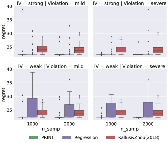
Figure 1: Boxplots of the regrets of learned pricing policy for 4 combinations of IV strength and violation of exclusion restriction.

6.2 Real Data Applications

In this subsection, we study the numerical performance of the pricing strategy of personalized loans for an anonymous US auto lending company. We compare our method by Kallus and Zhou (2018), a regression-based method, and the historical decision made by the company. A major difference between the real data application and the previous simulation study is that the structural equations (5) and (6) are potentially misspecified in the real data.

We obtain the dataset CPRM-12-001: On-Line Auto Lending from the Center for Pricing and Revenue Management at Columbia University. It records the online auto loan applications received by the company from Jul. 2002 to Nov. 2004. For each approved application, the requested term, loan amount, annual percentage rate (APR), monthly London interbank offered rate (LIBOR), whether contracted or not, and some personal information (e.g., FICO score) are recorded. For detailed descriptions, we refer the readers to Phillips et al. (2015) and Ban and Keskin (2021, Table 3).

6.2.1 Problem Settings and Evaluation Method

For the pricing of the online auto loan company, we adopt the price defined in Ban and Keskin (2021), which is the net present value of future payments less the loan amount, i.e.,

$$P=\text{Monthly Payment}\times\sum_{\tau=1}^{\text{Term}}(1+\text{monthly LIBOR})^{-\tau}-\text{Loan Amount}.$$ (18)

We set the feasible price range to be $[\$0,\$40,000]$.

To evaluate the pricing policy, it is necessary to construct a generative model since the revenue depends on the price selected by the policy, which is not available in the dataset. This is in contrast to supervised learning, where a testing dataset can be used to evaluate prediction accuracy. Since the outcomes of whether contracted or not are binary (accept/reject), instead of a linear demand, we adopt a logistic demand model used by Ban and Keskin (2021) for generating the demand. Therefore the true expected revenue is not a quadratic function of the price, conditioning on other factors. While this causes a model mis-specification for our method, we indeed find that our method works well and is robust to such a mis-specified revenue model. In addition, this serves as a complement to the previous simulation study, where we studied a correctly specified model. In particular, for a given feature vector $x$ (including the constant term) and a price $p$, the probability of accepting the contract, i.e., the expected demand, is modeled by $\frac{1}{1+\exp\{-\alpha^{\top}x-\beta^{\top}x\times p\}}.$ Then the expected revenue is $p/[1+\exp\{-\alpha^{\top}x-\beta^{\top}x\times p\}]$. The population demand model, which will be used to evaluate the revenue, is obtained by fitting a logistic regression with $\ell^{2}$-penalty with all records. We select the penalty parameter by 5-fold cross-validation.

6.2.2 Implementation

It is worth noting that even a competitor’s rate is available in this dataset. In practice, however, we actually do not have reliable data to represent the competition in the auto lending industry during the analyzed period of time (Phillips et al., 2015). Therefore, we intentionally treat the competitor’s rate as an unmeasured confounding and exclude it from the feature vector. Further, given the loan amount, term, and LIBOR, the price of a loan can be purely determined by the monthly payment. Therefore, to ensure that Assumption 2 (a) holds, we also exclude the monthly payment from the feature vector.

For PRINT, we choose the APR (annual percentage rate) for a loan as the instrumental variable, which was used as the instrument for dealing with the endogeneity of the price by Blundell-Wignall et al. (1992). Meanwhile, the loan rate is continuous and has a strong direct effect on the continuous price, which indicates that it could be used as a strong relevant IV. However, using the loan rate as a valid IV is questionable, since it may have a direct effect on the eventual revenue, hence breaking the IV exclusion restriction. However, we can safely use the loan APR as the invalid IV for our method since the IV exclusion restriction has been relaxed.

For comparison, in addition to the two benchmark methods compared in Section 6.1, we also consider the company’s actual pricing policy and the optimal policy by maximizing the revenue according to the learned population demand model. We use the first 60,000 records (ordered by application time) of the dataset as the training data to learn the policies for PRINT and two benchmark methods. Then we apply those learned policies to the testing dataset of the rest 148,084 records and calculate the revenues by the learned demand model.

6.2.3 Results and Discussion

Table 1 summarizes the expected revenue for the pricing policy learned by the PRINT against the benchmark policies, optimal policy, and policy used by the firm. The firm’s historical policy could attain 77.3% of the revenue if the optimal policy were used. This satisfactory revenue is reasonable since the firm may have external information at the pricing time that is not available in the offline records. The expected revenues obtained by the policies learned by direct regression and Kallus and Zhou (2018) do not reach the firm’s historical revenue, partially because of the unobserved confounding issue and insufficient offline data. In contrast, the policy learned by PRINT attains about 82.3% of the expected revenue of the optimal policy and improves the firm’s revenue by 6.5%.

Table 1: Values of pricing policies on the testing dataset.

Pricing Policy	Optimal	Firm	PRINT	Kallus and Zhou (2018)	Regression
Revenue ($1000)	1.0766	0.8318	0.8858	0.1452	0.0913

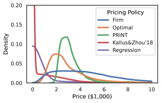
Figure 2: Personalized Pricing distributions on the testing dataset.

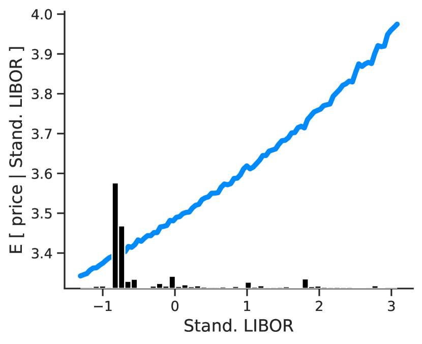
(a) LIBOR

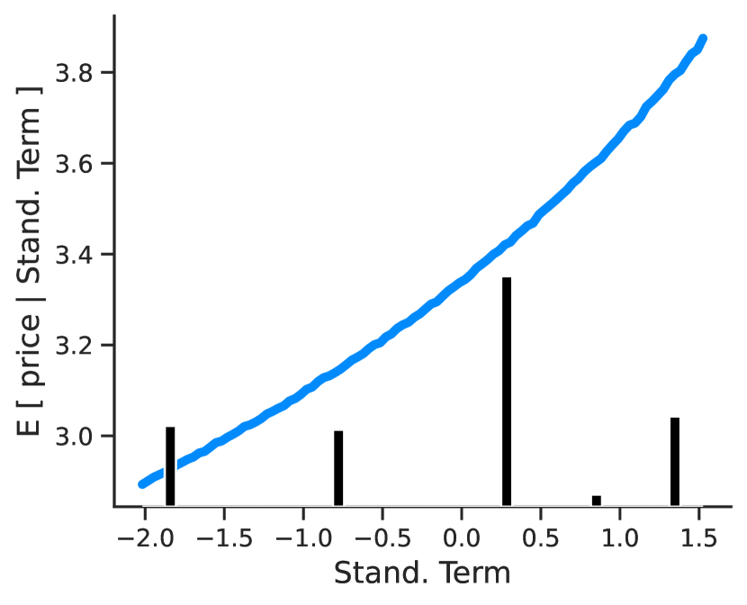
(b) Term

(c) FICO score

(d) Days until approval

Figure 3: Partial dependence plots of by pricing strategy by PRINT on important factors. All factors are standardized by their mean and standard deviation, respectively.

In Figure 2, we provide the density plots of the prices by the five pricing policies on the testing dataset. It is clear that the distribution of prices suggested by PRINT is the closest to the oracle optimal policy.

To study the interpretability of the policy learned by PRINT, in Figure 3, we provide the partial dependence plots of the learned policy on the four most important features. First, as shown in Figure 3(a) and (b), the price increases with LIBOR and term, which agrees with the definition of the price in (18). Second, Figure 3(c) shows that for customers with higher FICO scores, we suggest lower prices as those customers have low risks of bad debts. Finally, as shown in Figure 3(d), our policy tends to set higher prices for the applications with longer processing times, this is likely because those applications have potential risks that require longer review processes.

7 Conclusions

In this paper, we study offline personalized pricing under endogeneity by leveraging an instrumental variable. The key challenges are (a) identification of the heterogeneous effect of continuous price on revenue under unmeasured confounding; (b) a possibly invalid IV that may violate the exclusion restriction; (c) solving conditional moment restrictions of generalized residual functions. For (a) and (b), we generalized the identification results in causal inference literature on relaxing exclusion restriction for discrete treatment to continuous treatment. For (c), we develop an adversarial min-max algorithm for learning the optimal pricing strategy. Theoretically, we established the consistency and the convergence rate of the proposed policy learning algorithm. For future work, it is interesting to extend our work to learning a multi-stage policy strategy with offline data under endogeneity with invalid IVs.

Appendix A A Detailed Practical Algorithm

In this section, we give a detailed practical implementation of Algorithm 1 when the function classes ${\mathcal{H}}$ and ${\mathcal{F}}$ are neural networks (NNs), in which the functions can be parameterized by some NN parameters. Specifically, suppose that ${\mathcal{H}}=\{\alpha_{\theta_{\alpha}}(\bullet)=\alpha(\bullet;\theta_{\alpha}):\theta_{\alpha}\in\Theta_{{\mathcal{H}}}\}$ and that ${\mathcal{F}}=\{f_{\theta_{f}}(\bullet)=f(\bullet;\theta_{f}):\theta_{f}\in\Theta_{{\mathcal{F}}}\}$ for some Euclidean subspaces $\Theta_{{\mathcal{H}}}$ and $\Theta_{{\mathcal{F}}}$. In the case of a large sample size, one can apply the stochastic gradient ascent/descent with sub-sampled mini-batch data from the total batch data ${\mathcal{D}}_{n}$ in each iteration in Algorithm 1. Instead of updating $\widehat{f}^{(k)}$ and $\widehat{\alpha}^{(k)}$ by the respective optimization points, we can apply one-step update in each iteration. See details in Algorithm 2.

Input: Batch data ${\mathcal{D}}_{n}=\left\{Z_{i}=(Y_{i},X_{i},G_{i},P_{i})\right\}_{i=1}^{n}$. Initial $\widehat{\theta}_{f}^{(-1)},\widehat{\theta}_{\alpha}^{(0)}$. Tuning parameters $\lambda_{n_{B}},\mu_{n_{B}}>0$. Price range $[p_{1},p_{2}]$. Maximum iteration $K$. Batch size $1\leq n_{B}\leq n$. Step sizes $\gamma_{\alpha},\gamma_{f}>0.$

For $k\in\left\{0,\dots,K-1\right\}$:

Randomly sample a mini-batch $D_{I}=\left\{Z_{i}\right\}_{i\in I}$ with $|I|=n_{B}$.

$$\widehat{\theta}_{f}^{(k)}\leftarrow\widehat{\theta}_{f}^{(k)}+\gamma_{f}\nabla_{\theta_{f}}\left[\Psi_{n_{B}}(\alpha_{\widehat{\theta}_{\alpha}^{(k)}},f_{\widehat{\theta}_{f}^{(k-1)}})-\|f_{\widehat{\theta}_{f}^{(k-1)}}\|_{\alpha_{\widehat{\theta}_{\alpha}^{(k)}},n_{B}}^{2}-\lambda_{n_{B}}\|f_{\widehat{\theta}_{f}^{(k-1)}}\|_{\mathcal{F}}^{2}\right];$$

$\widehat{\theta}_{\alpha}^{(k+1)}\leftarrow\widehat{\theta}_{\alpha}^{(k)}-\gamma_{\alpha}\nabla_{\theta_{\alpha}}\left[\Psi_{n_{B}}(\alpha_{\widehat{\theta}_{\alpha}^{(k)}},f_{\widehat{\theta}_{f}^{(k)}})+\mu_{n_{B}}\|\alpha_{\widehat{\theta}_{\alpha}^{(k)}}\|_{\mathcal{H}}^{2}\right]$;

End For

Output: Pricing policy $\widehat{\pi}=\min\{\max\{p_{1},-\widehat{\beta}_{p,1}^{(K)}/[2\widehat{\beta}_{p,2}^{(K)}]\},p_{2}\}$.

Algorithm 2 Estimation of $\widehat{\pi}$ by solving a zero-sum game.

Appendix B Details of Numerical Study

Following the data generating procedure in Section 6.1, the ground truth nuisance functions of policy are

$$\widetilde{\beta}_{p,1}(X) =\mathbb{E}\left[\beta_{p,1}(U,X)\,|\,X\right]=-c_{1}^{\top}X+(\mu_{u_{1}}+c_{u_{1}}^{\top}X)^{2}+\sigma_{u_{1}}^{2},$$

$$\widetilde{\beta}_{p,2}(X) =\mathbb{E}\left[\beta_{p,2}(U,X)\,|\,X\right]=-\exp\left\{\mu_{u_{1}}+\sigma_{u_{1}}^{2}/2+(c_{2}+c_{u_{1}})^{\top}X\right\}.$$

Then the oracle optimal pricing policy is

$$\pi^{*}(X) =\min\left\{p_{2},\max\left\{p_{1},-\widetilde{\beta}_{p,1}(X)/\widetilde{\beta}_{p,2}(X)\right\}\right\}$$

$$=\min\left\{p_{2},\max\left\{p_{1},\frac{-c_{1}^{\top}X+(\mu_{u_{1}}+c_{u_{1}}^{\top}X)^{2}+\sigma_{u_{1}}^{2}}{\exp\left\{\mu_{u_{1}}+\sigma_{u_{1}}^{2}/2+(c_{2}+c_{u_{1}})^{\top}X\right\}}\right\}\right\}.$$

All parameters used for the data generating procedure are listed in Table 2.

Table 2: Simulation data parameters.

Parameter	$\mu_{x}$	$\Sigma_{x}$	$\mu_{g}$	$\mu_{u_{1}}$	$\mu_{u_{2}}$
Value	$[0.25,0.25]^{\top}$	$\text{diag}(1,1)$	$2$	$0.5$	$0.3$
Parameter	$c_{g}$	$c_{u_{1}}$	$c_{u_{2}}$	$\sigma_{g}^{2}$	$\sigma_{u_{1}}^{2}$
Value	$[0.25,0.25]^{\top}$	$[0.3,0.4]^{\top}$	$[0.2,0.2]^{\top}$	1	3
Parameter	$\sigma_{u_{2}}^{2}$	$c_{1}$	$c_{2}$	$c_{3}$	$c_{4}$
Value	1	$[0.3,0.2]^{\top}$	$[0.1,-0.3]^{\top}$	$[0.2,-0.1]^{\top}$	1 or 5
Parameter	$c_{5}$	$c_{6}$	$c_{7}$
Value	$[0.4,0.1]^{\top}$	$[1.2,0.4]^{\top}$	1 or 5

Appendix C Technical Proofs

C.1 Proof of Identification Results.

Proof of Lemma 1.. Without loss of generality, we assume $X=\emptyset$. By direct calculation, we have

$$\mathbb{E}\left[(G-\mathbb{E}\left[G\right])(P-\mathbb{E}\left[P\,|\,G\right])Y\right]$$

$$\ =\mathbb{E}\left[(G-\mathbb{E}\left[G\right])(P-\mathbb{E}\left[P\,|\,G\right])\left\{P\beta_{p,1}(U)+P^{2}\beta_{p,2}(U)+\beta_{g}(U,G)+\beta_{u}(U)\right\}\right]$$

$$\ =\mathbb{E}\left[(G-\mathbb{E}\left[G\right])(P-\mathbb{E}\left[P\,|\,G\right])P\right]\times\mathbb{E}\left[\beta_{p,1}(U)\right]$$

$$\quad+\mathbb{E}\left[(G-\mathbb{E}\left[G\right])(P-\mathbb{E}\left[P\,|\,G\right])P\left(\beta_{p,1}(U)-\mathbb{E}\left[\beta_{p,1}(U)\right]\right)\right]$$ (L1.A)

$$\quad+\mathbb{E}\left[(G-\mathbb{E}\left[G\right])(P-\mathbb{E}\left[P\,|\,G\right])P^{2}\right]\times\mathbb{E}\left[\beta_{p,2}(U)\right]$$

$$\quad+\mathbb{E}\left[(G-\mathbb{E}\left[G\right])(P-\mathbb{E}\left[P\,|\,G\right])P^{2}\left(\beta_{p,2}(U)-\mathbb{E}\left[\beta_{p,2}(U)\right]\right)\right]$$ (L1.B)

$$\quad+\mathbb{E}\left[(G-\mathbb{E}\left[G\right])(P-\mathbb{E}\left[P\,|\,G\right])\left\{\beta_{g}(U,G)+\beta_{u}(U)\right\}\right].$$ (L1.C)

It suffices to prove that (L1.A) – (L1.C) are zeros. By direct calculations,

(L1.A) $$=\mathbb{E}\left[(G-\mathbb{E}\left[G\right])(P-\mathbb{E}\left[P\,|\,G\right])P\left(\beta_{p,1}(U)-\mathbb{E}\left[\beta_{p,1}(U)\right]\right)\right]$$

$$\ =\mathbb{E}\left[(G-\mathbb{E}\left[G\right])P^{2}\left(\beta_{p,1}(U)-\mathbb{E}\left[\beta_{p,1}(U)\right]\right)\right]$$

$$\quad-\mathbb{E}\left[(G-\mathbb{E}\left[G\right])\mathbb{E}\left[P\,|\,G\right]P\left(\beta_{p,1}(U)-\mathbb{E}\left[\beta_{p,1}(U)\right]\right)\right]$$

$$=\mathbb{E}\left[(G-\mathbb{E}\left[G\right]){\mbox{Cov}}(\beta_{p,1}(U),\mathbb{E}\left[P^{2}\,|\,U,G\right])\,|\,G\right]$$

$$\quad-\mathbb{E}\left[(G-\mathbb{E}\left[G\right])\mathbb{E}\left[P\,|\,G\right]\left(\alpha_{g}(U,G)+\alpha_{u,x}(U)\right)\left(\beta_{p,1}(U)-\mathbb{E}\left[\beta_{p,1}(U)\right]\right)\right]$$

$$\ =\mathbb{E}\left[(G-\mathbb{E}\left[G\right])\mathbb{E}\left[P\,|\,G\right]{\mbox{Cov}}\left(\alpha_{g}(U,G),\beta_{p,1}(U)\,|\,G\right)\right]$$

$$\quad+\mathbb{E}\left[(G-\mathbb{E}\left[G\right])\mathbb{E}\left[P\,|\,G\right]{\mbox{Cov}}\left(\alpha_{u,x}(U),\beta_{p,1}(U)\,|\,G\right)\right]$$

$$\ =0.$$

Similarly, we can show that

(L1.B) $$=\mathbb{E}\left[(G-\mathbb{E}\left[G\right])(P-\mathbb{E}\left[P\,|\,G\right])P^{2}\left(\beta_{p,2}(U)-\mathbb{E}\left[\beta_{p,2}(U)\right]\right)\right]$$

$$\ =\mathbb{E}\left[(G-\mathbb{E}\left[G\right])P^{3}\left(\beta_{p,2}(U)-\mathbb{E}\left[\beta_{p,2}(U)\right]\right)\right]$$

$$\quad-\mathbb{E}\left[(G-\mathbb{E}\left[G\right])\mathbb{E}\left[P\,|\,G\right]P^{2}\left(\beta_{p,2}(U)-\mathbb{E}\left[\beta_{p,2}(U)\right]\right)\right]$$

$$\ =\mathbb{E}\left[(G-\mathbb{E}\left[G\right]){\mbox{Cov}}(\beta_{p,2}(U),\mathbb{E}\left[P^{3}\,|\,U,G\right])\,|\,G\right]$$

$$\ =0.$$

Lastly, we show that

(L1.C) $$=\mathbb{E}\left[(G-\mathbb{E}\left[G\right])(P-\mathbb{E}\left[P\,|\,G\right])\left\{\beta_{g}(U,G)+\beta_{u}(U)\right\}\right]$$

$$\ =\mathbb{E}\left[(G-\mathbb{E}\left[G\right])(\alpha_{g}(U,G)-\mathbb{E}\left[\alpha_{g}(U,G)\,|\,G\right])\left\{\beta_{g}(U,G)+\beta_{u}(U)\right\}\right]$$

$$\quad+\mathbb{E}\left[(G-\mathbb{E}\left[G\right])(\alpha_{u,x}(U)-\mathbb{E}\left[\alpha_{u,x}(U)\right])\left\{\beta_{g}(U,G)+\beta_{u}(U)\right\}\right]$$

$$=\mathbb{E}\left[(G-\mathbb{E}\left[G\right])\left\{{\mbox{Cov}}(\alpha_{g}(U,G),\beta_{g}(U,G)\,|\,G)+{\mbox{Cov}}(\alpha_{g}(U,G),\beta_{u}(U)\,|\,G)\right\}\right]$$

$$\quad+\mathbb{E}\left[(G-\mathbb{E}\left[G\right])\left\{{\mbox{Cov}}(\alpha_{u,x}(U),\beta_{g}(U,G)\,|\,G)+{\mbox{Cov}}(\alpha_{u,x}(U)),\beta_{u}(U)\,|\,G)\right\}\right]$$

$$\ =0.$$

 

Proof of Lemma 2.. Without loss of generality, we assume $X=\emptyset$. By direct calculation, we have

$$\mathbb{E}\left[G(G-\mathbb{E}\left[G\right])(P-\mathbb{E}\left[P\,|\,G\right])Y\right]$$

$$\ =\mathbb{E}\left[G(G-\mathbb{E}\left[G\right])(P-\mathbb{E}\left[P\,|\,G\right])\left\{P\beta_{p,1}(U)+P^{2}\beta_{p,2}(U)+\beta_{g}(U,G)+\beta_{u}(U)\right\}\right]$$

$$\ =\mathbb{E}\left[G(G-\mathbb{E}\left[G\right])(P-\mathbb{E}\left[P\,|\,G\right])P\right]\times\mathbb{E}\left[\beta_{p,1}(U)\right]$$

$$\quad+\mathbb{E}\left[G(G-\mathbb{E}\left[G\right])(P-\mathbb{E}\left[P\,|\,G\right])P\left(\beta_{p,1}(U)-\mathbb{E}\left[\beta_{p,1}(U)\right]\right)\right]$$ (L2.A)

$$\quad+\mathbb{E}\left[(G-\mathbb{E}\left[G\right])(P-\mathbb{E}\left[P\,|\,G\right])P^{2}\right]\times\mathbb{E}\left[\beta_{p,2}(U)\right]$$

$$\quad+\mathbb{E}\left[G(G-\mathbb{E}\left[G\right])(P-\mathbb{E}\left[P\,|\,G\right])P^{2}\left(\beta_{p,2}(U)-\mathbb{E}\left[\beta_{p,2}(U)\right]\right)\right]$$ (L2.B)

$$\quad+\mathbb{E}\left[G(G-\mathbb{E}\left[G\right])(P-\mathbb{E}\left[P\,|\,G\right])\left\{\beta_{g}(U,G)+\beta_{u}(U)\right\}\right].$$ (L2.C)

Note that

(L2.A) $$=\mathbb{E}\left[G(G-\mathbb{E}\left[G\right])(P-\mathbb{E}\left[P\,|\,G\right])P\left(\beta_{p,1}(U)-\mathbb{E}\left[\beta_{p,1}(U)\right]\right)\right]$$

$$\ =\mathbb{E}\left[G(G-\mathbb{E}\left[G\right])P^{2}\left(\beta_{p,1}(U)-\mathbb{E}\left[\beta_{p,1}(U)\right]\right)\right]$$

$$\quad-\mathbb{E}\left[G(G-\mathbb{E}\left[G\right])\mathbb{E}\left[P\,|\,G\right]P\left(\beta_{p,1}(U)-\mathbb{E}\left[\beta_{p,1}(U)\right]\right)\right]$$

$$\ =\mathbb{E}\left[G(G-\mathbb{E}\left[G\right]){\mbox{Cov}}(\beta_{p,1}(U),\mathbb{E}\left[P^{2}\,|\,U,G\right])\,|\,G\right]$$

$$\quad-\mathbb{E}\left[G(G-\mathbb{E}\left[G\right])\mathbb{E}\left[P\,|\,G\right]\left(\alpha_{g}(U,G)+\alpha_{u,x}(U)\right)\left(\beta_{p,1}(U)-\mathbb{E}\left[\beta_{p,1}(U)\right]\right)\right]$$

$$\ =\mathbb{E}\left[G(G-\mathbb{E}\left[G\right])\mathbb{E}\left[P\,|\,G\right]{\mbox{Cov}}\left(\alpha_{g}(U,G),\beta_{p,1}(U)\,|\,G\right)\right]$$

$$\quad+\mathbb{E}\left[G(G-\mathbb{E}\left[G\right])\mathbb{E}\left[P\,|\,G\right]{\mbox{Cov}}\left(\alpha_{u,x}(U),\beta_{p,1}(U)\,|\,G\right)\right]$$

$$\ =0.$$

Similarly, we can show that

(L2.B) $$=\mathbb{E}\left[G(G-\mathbb{E}\left[G\right])(P-\mathbb{E}\left[P\,|\,G\right])P^{2}\left(\beta_{p,2}(U)-\mathbb{E}\left[\beta_{p,2}(U)\right]\right)\right]$$

$$\ =\mathbb{E}\left[G(G-\mathbb{E}\left[G\right])P^{3}\left(\beta_{p,2}(U)-\mathbb{E}\left[\beta_{p,2}(U)\right]\right)\right]$$

$$\quad-\mathbb{E}\left[G(G-\mathbb{E}\left[G\right])\mathbb{E}\left[P\,|\,G\right]P^{2}\left(\beta_{p,2}(U)-\mathbb{E}\left[\beta_{p,2}(U)\right]\right)\right]$$

$$\ =\mathbb{E}\left[G(G-\mathbb{E}\left[G\right]){\mbox{Cov}}(\beta_{p,2}(U),\mathbb{E}\left[P^{3}\,|\,U,G\right])\,|\,G\right]$$

$$=0.$$

Lastly, we can show that

(L2.C) $$=\mathbb{E}\left[G(G-\mathbb{E}\left[G\right])(P-\mathbb{E}\left[P\,|\,G\right])\left\{\beta_{g}(U,G)+\beta_{u}(U)\right\}\right]$$

$$\ =\mathbb{E}\left[G(G-\mathbb{E}\left[G\right])(\alpha_{g}(U,G)-\mathbb{E}\left[\alpha_{g}(U,G)\,|\,G\right])\left\{\beta_{g}(U,G)+\beta_{u}(U)\right\}\right]$$

$$\quad+\mathbb{E}\left[G(G-\mathbb{E}\left[G\right])(\alpha_{u,x}(U)-\mathbb{E}\left[\alpha_{u,x}(U)\right])\left\{\beta_{g}(U,G)+\beta_{u}(U)\right\}\right]$$

$$\ =\mathbb{E}\left[G(G-\mathbb{E}\left[G\right])\left\{{\mbox{Cov}}(\alpha_{g}(U,G),\beta_{g}(U,G)\,|\,G)+{\mbox{Cov}}(\alpha_{g}(U,G),\beta_{u}(U)\,|\,G)\right\}\right]$$

$$\quad+\mathbb{E}\left[G(G-\mathbb{E}\left[G\right])\left\{{\mbox{Cov}}(\alpha_{u,x}(U),\beta_{g}(U,G)\,|\,G)+{\mbox{Cov}}(\alpha_{u,x}(U),\beta_{u}(U)\,|\,G)\right\}\right]$$

$$\ =\mathbb{E}\left[G(G-\mathbb{E}\left[G\right])\right]{\mbox{Cov}}(\alpha_{u,x}(U),\beta_{u}(U)).$$

Summarizing the first equation with (L2.A) – (L2.C) together, we have that

$$\mathbb{E}\left[G(G-\mathbb{E}\left[G\right])(P-\mathbb{E}\left[P\,|\,G\right])Y\right]$$ (19)

$$\ =\mathbb{E}\left[G(G-\mathbb{E}\left[G\right])(P-\mathbb{E}\left[P\,|\,G\right])P\right]\times\mathbb{E}\left[\beta_{p,1}(U)\right]$$

$$\quad+\mathbb{E}\left[G(G-\mathbb{E}\left[G\,|\,X\right])(P-\mathbb{E}\left[P\,|\,G\right])P^{2}\right]\times\mathbb{E}\left[\beta_{p,2}(U)\right]$$

$$\quad+\mathbb{E}\left[G(G-\mathbb{E}\left[G\right])\right]{\mbox{Cov}}(\alpha_{u,x}(U),\beta_{u}(U)).$$

Next, we derive that

$$\mathbb{E}\left[(P-\mathbb{E}\left[P\,|\,G\right])Y\right]$$ (20)

$$\ =\mathbb{E}\left[(P-\mathbb{E}\left[P\,|\,G\right])\left\{\beta_{p,1}(U)P+\beta_{p,2}(U)P^{2}+\beta_{g}(U,G)+\beta_{u}(U)\right\}\right]$$

$$\ =\mathbb{E}\left[P(P-\mathbb{E}\left[P\,|\,G\right])\right]\times\mathbb{E}\left[\beta_{p,1}(U)\right]+\mathbb{E}\left[P^{2}(P-\mathbb{E}\left[P\,|\,G\right])\right]\times\mathbb{E}\left[\beta_{p,2}(U)\right]$$

$$\quad+{\mbox{Cov}}(\alpha_{u}(U),\beta_{u}(U)).$$

By substituting (20) into (19), we obtain that

$$\mathbb{E}\left[G(G-\mathbb{E}\left[G\right])(P-\mathbb{E}\left[P\,|\,G\right])Y\right]$$

$$\ =\mathbb{E}\left[G(G-\mathbb{E}\left[G\right])(P-\mathbb{E}\left[P\,|\,G\right])P\right]\times\mathbb{E}\left[\beta_{p,1}(U)\right]$$

$$\quad+\mathbb{E}\left[G(G-\mathbb{E}\left[G\right])(P-\mathbb{E}\left[P\,|\,G\right])P^{2}\right]\times\mathbb{E}\left[\beta_{p,2}(U)\right]$$

$$\quad+\mathbb{E}\left[G(G-\mathbb{E}\left[G\right])\right]$$

$$\qquad\times\left\{\mathbb{E}\left[(P-\mathbb{E}\left[P\,|\,G\right])Y\right]-\mathbb{E}\left[P(P-\mathbb{E}\left[P\,|\,G\right])\right]\times\mathbb{E}\left[\beta_{p,1}(U)\right]\right.$$

$$\qquad\qquad\qquad\qquad\qquad\qquad\left.-\mathbb{E}\left[P^{2}(P-\mathbb{E}\left[P\,|\,G\right])\right]\times\mathbb{E}\left[\beta_{p,2}(U)\right]\right\}$$

$$\ ={\mbox{Cov}}(G(G-\mathbb{E}\left[G\right]),P(P-\mathbb{E}\left[P\,|\,G\right]))\mathbb{E}\left[\beta_{p,1}(U)\right]$$

$$\quad+{\mbox{Cov}}(G(G-\mathbb{E}\left[G\right]),P^{2}(P-\mathbb{E}\left[P\,|\,G\right]))\mathbb{E}\left[\beta_{p,2}(U)\right]$$

$$\quad+\mathbb{E}\left[G(G-\mathbb{E}\left[G\right])\right]\times\mathbb{E}\left[(P-\mathbb{E}\left[P\,|\,G\right])Y\right],$$

which concludes our proof.    

C.2 Proof of Estimation and Policy Learning

C.2.1 Proof of Consistency

Proof of Lemma 5. First, by Lemma 10, $\|\widehat{\alpha}_{n}\|_{\mathcal{H}}=\mathop{}\mathopen{}\mathcal{O}\mathopen{}_{\mathrm{p}}(1)$. We consider

$${\mbox{Pr}}\left[\|\widehat{\alpha}_{n}-\alpha_{0}\|_{2,2}>\epsilon\right]\leq{\mbox{Pr}}\left[\|\widehat{\alpha}_{n}-\alpha_{0}\|_{2,2}>\epsilon,\|\widehat{\alpha}_{n}\|_{\mathcal{H}}^{2}\leq M_{0}\right]+{\mbox{Pr}}\left[\|\widehat{\alpha}_{n}\|_{\mathcal{H}}^{2}>M_{0}\right].$$ (21)

For any $b>0$, we select $M_{0}\triangleq M_{0}(b)$ such that ${\mbox{Pr}}\left[\|\widehat{\alpha}_{n}\|_{\mathcal{H}}^{2}>M_{0}\right]<b$ for sufficiently large $n$ (by Lemma 10). We only need to focus on the set ${\mathcal{H}}_{M_{0}}\triangleq\left\{\alpha\in{\mathcal{H}}:\|\alpha\|_{\mathcal{H}}^{2}\leq M_{0}\right\}$. For the first part on the RHS of the inequality (21),

$${\mbox{Pr}}\left[\|\widehat{\alpha}_{n}-\alpha_{0}\|_{2,2}>\epsilon,\|\widehat{\alpha}_{n}\|_{\mathcal{H}}^{2}\leq M_{0}\right]$$ (22)

$$\ ={\mbox{Pr}}\left[\|\widehat{\alpha}_{n}-\alpha_{0}\|_{2,2}>\epsilon,\|\widehat{\alpha}_{n}\|_{\mathcal{H}}^{2}\leq M_{0},\widehat{\Phi}_{n}(\widehat{\alpha}_{n})\leq\inf_{\alpha\in{\mathcal{H}}}\widehat{\Phi}_{n}(\alpha)+\mathop{}\mathopen{}\mathcal{O}\mathopen{}_{\mathrm{p}}(\eta_{n})\right]$$

$$\ \leq{\mbox{Pr}}\left[\inf_{\alpha\in{\mathcal{H}}_{M_{0}}:\|\alpha-\alpha_{0}\|_{2,2}>\epsilon}\widehat{\Phi}_{n}(\alpha)\leq\inf_{\alpha\in{\mathcal{H}}}\widehat{\Phi}_{n}(\alpha)+\mathop{}\mathopen{}\mathcal{O}\mathopen{}_{\mathrm{p}}(\eta_{n})\right]$$

$$\ \leq{\mbox{Pr}}\left[\inf_{\alpha\in{\mathcal{H}}_{M_{0}}:\|\alpha-\alpha_{0}\|_{2,2}>\epsilon}\widehat{\Phi}_{n}(\alpha)\leq\widehat{\Phi}_{n}(\alpha_{0})+\mathop{}\mathopen{}\mathcal{O}\mathopen{}_{\mathrm{p}}(\eta_{n})\right]$$

$$\ \leq{\mbox{Pr}}\begin{bmatrix}[r]\min\left\{\frac{\delta_{n}}{2\sqrt{c_{\eta_{\Sigma}}}}\sqrt{\inf_{\alpha\in{\mathcal{H}}_{M_{0}}:\|\alpha-\alpha_{0}\|_{2,2}>\epsilon}\Phi(\alpha)},\inf_{\alpha\in{\mathcal{H}}_{M_{0}}:\|\alpha-\alpha_{0}\|_{2,2}>\epsilon}\frac{\Phi(\alpha)}{c_{\eta_{\Sigma}}}\right\}\\ \leq\mathop{}\mathopen{}\mathcal{O}\mathopen{}_{\mathrm{p}}(\max\left\{\delta_{n}^{2},\eta_{n}\right\})\end{bmatrix}$$

where the first equality is due to Assumption 6, the first inequality follows by the definition of $\widehat{\alpha}_{n}$ and relaxing conditions of the event, the second inequality is due to optimality, and the last inequality follows by Lemma 9.

Let $\varphi_{0}(\epsilon)=\inf_{\alpha\in{\mathcal{H}}_{M_{0}}:\|\alpha-\alpha_{0}\|_{2,2}>\epsilon}\sqrt{\Phi(\alpha)}$, which is strictly positive since $\|\alpha_{0}-\alpha\|_{2,2}=0$ only if $\Phi(\alpha)=0$ for $\alpha\in{\mathcal{H}}$. Then, with the Assumption 7 that $\eta_{n}\asymp\delta_{n}^{2}$, we have that

$${\mbox{Pr}}\left[\|\widehat{\alpha}_{n}-\alpha_{0}\|_{2,2}>\epsilon,\|\widehat{\alpha}_{n}\|_{\mathcal{H}}^{2}\leq M_{0}\right]$$

$$\leq{\mbox{Pr}}\left[\min\left\{\frac{\delta_{n}}{2\sqrt{c_{\eta_{\Sigma}}}}\varphi_{0}(\epsilon),\frac{\varphi_{0}(\epsilon)^{2}}{c_{\eta_{\Sigma}}}\right\}\leq\mathop{}\mathopen{}\mathcal{O}\mathopen{}_{\mathrm{p}}(\delta_{n}^{2})\right]\rightarrow 0,\text{ as }n\rightarrow\infty.$$

Then by letting $b\downarrow 0$, we have that ${\mbox{Pr}}\left[\|\widehat{\alpha}_{n}-\alpha_{0}\|_{2,2}>\epsilon\right]\rightarrow 0$ for any $\epsilon>0$.    

C.2.2 Proof for Convergence Rates

Proof of Theorem 2.. For all $M>1$, suppose $\left\{r_{n}\right\}$ is a sequence of non-increasing positive numbers. Let $\widetilde{{\mathcal{H}}}={\mathcal{H}}_{\alpha_{0},M_{0},\epsilon}$ for simplicity. By similar arguments of (22) in the proof of Lemma 5,

$${\mbox{Pr}}\left[\|\widehat{\alpha}_{n}-\alpha_{0}\|_{ps,\alpha_{0}}\geq Mr_{n},\widehat{\alpha}_{n}\in\widetilde{\mathcal{H}}\right]$$ (23)

$$\ \leq{\mbox{Pr}}\left[\inf_{\alpha\in\widetilde{\mathcal{H}}:\|\alpha-\alpha_{0}\|_{ps,\alpha_{0}}\geq Mr_{n}}\widehat{\Phi}_{n}(\alpha)\leq\widehat{\Phi}_{n}(\alpha_{0})+\mathop{}\mathopen{}\mathcal{O}\mathopen{}_{\mathrm{p}}(\eta_{n})\right]$$

$$\ \leq{\mbox{Pr}}\begin{bmatrix}[r]\min\left\{\frac{\delta_{n}}{2\sqrt{c_{\eta_{\Sigma}}}}\sqrt{\inf_{\alpha\in\widetilde{\mathcal{H}}:\|\alpha-\alpha_{0}\|_{ps,\alpha_{0}}\geq Mr_{n}}\Phi(\alpha)},\inf_{\alpha\in\widetilde{\mathcal{H}}:\|\alpha-\alpha_{0}\|_{ps,\alpha_{0}}\geq Mr_{n}}\frac{\Phi(\alpha)}{c_{\eta_{\Sigma}}}\right\}\\ \leq\mathop{}\mathopen{}\mathcal{O}\mathopen{}_{\mathrm{p}}(\max\left\{\delta_{n}^{2},\eta_{n}\right\})\end{bmatrix}.$$

By Assumption 8 that $\|\alpha-\alpha_{0}\|_{ps,\alpha_{0}}^{2}\leq c_{\text{curv}}\Phi(\alpha)$ for any $\alpha\in\widetilde{{\mathcal{H}}}$, we have

$$\frac{\delta_{n}}{2\sqrt{c_{\eta_{\Sigma}}c_{\text{curv}}}}Mr_{n} \leq\frac{\delta_{n}}{2\sqrt{c_{\eta_{\Sigma}}}}\sqrt{\inf_{\alpha\in\widetilde{\mathcal{H}}:\|\alpha-\alpha_{0}\|_{ps,\alpha_{0}}\geq Mr_{n}}\Phi(\alpha)},\text{ and}$$

$$\frac{M^{2}r_{n}^{2}}{c_{\eta_{\Sigma}}c_{\text{curv}}} \leq\inf_{\alpha\in\widetilde{\mathcal{H}}:\|\alpha-\alpha_{0}\|_{ps,\alpha_{0}}\geq Mr_{n}}\frac{\Phi(\alpha)}{c_{\eta_{\Sigma}}}.$$

Therefore, by taking $r_{n}\asymp\delta_{n}$, the probability in LHS of (23) can be arbitrarily small as $M\rightarrow\infty$. Hence,

$$\|\widehat{\alpha}_{n}-\alpha_{0}\|_{ps,\alpha_{0}} =\mathop{}\mathopen{}\mathcal{O}\mathopen{}_{\mathrm{p}}(\delta_{n}),\text{ and }$$

$$\|\widehat{\alpha}_{n}-\alpha_{0}\|_{2,2} =\mathop{}\mathopen{}\mathcal{O}\mathopen{}_{\mathrm{p}}(\omega(\delta_{n},{\mathcal{H}}_{\alpha_{0},M_{0},\epsilon})),$$

where we directly apply the definition of local modulus of continuity.    

C.2.3 Proof of Regret Rates

Proof of Theorem 3.. By (7) and (14), the regret can be bounded by

$$\mathcal{V}(\pi^{*})-\mathcal{V}(\widehat{\pi}) =\left(\mathbb{E}^{\pi^{*}}-\mathbb{E}^{\widehat{\pi}}\right)\left\{\mathbb{E}[Y\,|\,X,G,P]\right\}$$ (24)

$$=\mathbb{E}\{\beta_{p,1}(X)[\pi^{*}(X)-\widehat{\pi}(X)]+\beta_{p,2}(X)[\pi^{*}(X)^{2}-\widehat{\pi}(X)^{2}]\}$$

$$=\mathbb{E}\left(\{\beta_{1,p}(X)+\beta_{2,p}(X)[\pi^{*}(X)+\widehat{\pi}(X)]\}[\pi^{*}(X)-\widehat{\pi}(X)]\right)$$

$$\leq\|\beta_{1,p}+\beta_{2,p}[\pi^{*}+\widehat{\pi}]\|_{2}\|\pi^{*}-\widehat{\pi}\|_{2}$$

$$\leq(\|\beta_{1,p}\|_{2}+2p_{2}\|\beta_{2,p}\|_{2})\|\pi^{*}-\widehat{\pi}\|_{2}$$

$$=C_{\beta}\|\pi^{*}-\widehat{\pi}\|_{2},$$

where $C_{\beta}\triangleq\|\beta_{1,p}\|_{2}+2p_{2}\|\beta_{2,p}\|_{2}>0$, the first inequality is due to the Cauchy-Schwartz inequality, and the second inequality is due to the triangle inequality and the upper bound of the policy price.

Since $-\beta_{p,2}\geq c_{p,2}$ for some constant $c_{p,2}>0$, we have that

$$\|\pi^{*}-\widehat{\pi}\|_{2} =\|\min\{\max\{p_{1},-\widehat{\beta}_{p,1}/[2\widehat{\beta}_{p,2}]\},p_{2}\}-\min\{\max\{p_{1},-\beta_{p,1}/[2\beta_{p,2}]\},p_{2}\}\|_{2}$$

$$\lesssim\frac{\max\{1,p_{2}\}}{2c_{p,2}}\left(\|[\beta_{1,p}-\widehat{\beta}_{1,p},\beta_{2,p}-\widehat{\beta}_{2,p}]\|_{2,2}\right)$$

$$\lesssim\|\widehat{\alpha}_{n}-\alpha_{0}\|_{2,2},$$

where the first inequality is due to the range of $\beta_{p,2}$ and that of policies in $\Pi$, and the second inequality follows by the definition of $\alpha$.

The results follow by directly applying the definition of local modulus of continuity.    

C.2.4 Proof of Results in RKHS cases

Then Corollary 1 is a direct consequence of Theorem 2 by Example 1 in Miao et al. (2022) and Lemma 11.

Proof of Corollary 2.. Corollary 2 can be obtained by directly applying Lemma 6 and Corollary 1.

Specifically, for part (a), i.e., the mild ill-posed case: given $\lambda_{m}(K_{{\mathcal{H}}})\sim m^{-2\gamma_{{\mathcal{H}}}}$ and $\tau_{m}\sim m^{-2b}$, then the optimum $m_{*}$ that solves

$$\min_{m\in{\mathbb{N}}_{+}}\frac{\eta^{2}}{\tau_{m}}+M_{0}\left[2c\sqrt{\sum_{i=1}^{\infty}\lambda_{i}(K_{{\mathcal{H}}})}\sqrt{\sum_{j=m+1}^{\infty}\lambda_{j}(K_{{\mathcal{H}}})}+\lambda_{m+1}(K_{{\mathcal{H}}})\right],$$

is such that $m_{*}\sim\left(\eta^{2}\right)^{-\frac{1}{2(\gamma_{{\mathcal{H}}}-1/2+b)}}$, and $\omega(\eta,{\mathcal{H}}_{M_{0}})^{2}\sim\left(\eta^{2}\right)^{\frac{\gamma_{{\mathcal{H}}}-1/2}{\gamma_{{\mathcal{H}}}-1/2+b}}$.

Thus, by Corollary 1 and Theorem 2, we have with probability at least $1-\zeta$,

$$\|\alpha-\alpha_{0}\|_{2,2} \lesssim\omega(n^{-\frac{1}{2+1/\min(\gamma_{{\mathcal{H}}},\gamma_{{\mathcal{F}}})}}\log(n)+\sqrt{\frac{\log(1/\zeta)}{n}},{\mathcal{H}}_{\alpha_{0},M_{0},\epsilon})$$

$$\lesssim\omega(n^{-\frac{1}{2+1/\min(\gamma_{{\mathcal{H}}},\gamma_{{\mathcal{F}}})}}\log(n)+\sqrt{\frac{\log(1/\zeta)}{n}},{\mathcal{H}}_{M_{0}})$$

$$\lesssim\left(n^{-\frac{1}{2+1/\min(\gamma_{{\mathcal{H}}},\gamma_{{\mathcal{F}}})}}\log(n)+\sqrt{\frac{\log(1/\zeta)}{n}}\right)^{\frac{\gamma_{{\mathcal{H}}}-1/2}{\gamma_{{\mathcal{H}}}-1/2+b}}.$$

Then the result follows by letting $\zeta=1/n$. By applying Theorem 3, ${\mathcal{V}}(\pi^{*})-{\mathcal{V}}(\widehat{\pi})=\mathop{}\mathopen{}\mathcal{O}\mathopen{}_{\mathrm{p}}\left(n^{-\frac{1}{2+1/\min(\gamma_{{\mathcal{H}}},\gamma_{{\mathcal{F}}})}}\log(n)\right)$.

For part (b), the severe ill-posed case, given $\lambda_{m}(K_{{\mathcal{H}}})\sim m^{-2\gamma_{{\mathcal{H}}}}$ and $\tau_{m}\sim e^{-m^{b}}$, we can similarly obtain that the optimum $m_{*}\sim[\log(1/\eta)]^{1/b}$, and $\omega(\eta,{\mathcal{H}}_{M_{0}})^{2}\sim\left[\log(1/\eta)\right]^{-\frac{2\gamma_{{\mathcal{H}}}-1}{b}}$. Thus, by Corollary 1 and Theorem 2, we have with probability at least $1-\zeta$,

$$\|\alpha-\alpha_{0}\|_{2,2} \lesssim\omega(n^{-\frac{1}{2+1/\min(\gamma_{{\mathcal{H}}},\gamma_{{\mathcal{F}}})}}\log(n)+\sqrt{\frac{\log(1/\zeta)}{n}},{\mathcal{H}}_{\alpha_{0},M_{0},\epsilon})$$

$$\lesssim\omega(n^{-\frac{1}{2+1/\min(\gamma_{{\mathcal{H}}},\gamma_{{\mathcal{F}}})}}\log(n)+\sqrt{\frac{\log(1/\zeta)}{n}},{\mathcal{H}}_{M_{0}})$$

$$\lesssim\left(\log n\right)^{-\frac{\gamma_{{\mathcal{H}}}-1/2}{2b}}.$$

By applying Theorem 3, ${\mathcal{V}}(\pi^{*})-{\mathcal{V}}(\widehat{\pi})=\mathop{}\mathopen{}\mathcal{O}\mathopen{}_{\mathrm{p}}\left(\left(\log n\right)^{-\frac{\gamma_{{\mathcal{H}}}-1/2}{2b}}\right)$.    

C.3 Additional Lemmas

Lemma 7

(Relating empirical and population regularization) For any given $\widetilde{\alpha}\in{\mathcal{H}}$, we have that with probability at least $1-\zeta$, uniformly for all $f\in{\mathcal{F}}$,

$$\left|\|f\|_{n,\widetilde{\alpha}}^{2}-\|f\|_{\widetilde{\alpha}}^{2}\right|\leq\frac{1}{2}\|f\|_{\widetilde{\alpha}}^{2}+\delta_{n}^{2}\max\left\{1,\frac{\|f\|_{\mathcal{F}}^{2}}{B}\right\},$$ (25)

where $\delta_{n}=\bar{\delta}_{n}+\mathop{}\mathopen{}\mathcal{O}\mathopen{}(\sqrt{\frac{\log(1/\zeta)}{n}})$ and $\bar{\delta}_{n}$ upper bounds the critical radius of class ${\mathcal{F}}_{B}\times W(\bullet;\widetilde{\alpha})$. When $\lambda_{n}\geq\frac{2\delta_{n}^{2}}{B}$, with probability at least $1-\zeta$, uniformly for all $f\in{\mathcal{F}}$,

$$\lambda_{n}\|f\|_{\mathcal{F}}^{2}+\|f\|_{n,\widetilde{\alpha}}^{2}\geq\frac{\lambda_{n}}{2}\|f\|_{\mathcal{F}}^{2}+\frac{1}{2}\|f\|_{\widetilde{\alpha}}^{2}-\delta_{n}^{2}.$$ (26)

Lemma 8

(Relating $\Psi_{n}$ and $\Psi$)

1. For any fixed $\alpha\in{\mathcal{H}}$, let $\delta_{n}=\bar{\delta}_{n}+\mathop{}\mathopen{}\mathcal{O}\mathopen{}(\sqrt{\frac{\log(1/\zeta)}{n}})$ with $\bar{\delta}_{n}$ upper bounds the critical radius of the class $W(\cdot,\alpha)\times{\mathcal{F}}_{B}$. Then with probability at least $1-\zeta$, uniformly for all $f\in{\mathcal{F}}$,

   $$\left|\Psi_{n}(\alpha,f)-\Psi(\alpha,f)\right|\leq\mathop{}\mathopen{}\mathcal{O}\mathopen{}\left(\delta_{n}\|f\|_{2,2}+\delta_{n}^{2}\max\left\{1,\frac{\|f\|_{\mathcal{F}}}{\sqrt{B}}\right\}\right).$$

2. Given $M_{0}>0$, uniformly for all $\alpha\in{\mathcal{H}}_{M_{0}}\subset{\mathcal{H}}$, let $\delta_{n}=\bar{\delta}_{n}+\mathop{}\mathopen{}\mathcal{O}\mathopen{}(\sqrt{\frac{\log(1/\zeta)}{n}})$ with $\bar{\delta}_{n}$ upper bounds the critical radius of the class

   $$\left\{W(\cdot,\alpha)f(*):\alpha\in{\mathcal{H}}_{M_{0}},f\in{\mathcal{F}}_{B}\right\}.$$

   Then with probability at least $1-\zeta$, uniformly for all $f\in{\mathcal{F}}$ and $h\in{\mathcal{H}}_{M_{0}}$,

   $$\left|\Psi_{n}(\alpha,f)-\Psi(\alpha,f)\right|\leq\mathop{}\mathopen{}\mathcal{O}\mathopen{}\left(\delta_{n}\|f\|_{2,2}+\delta_{n}^{2}\max\left\{1,\frac{\|f\|_{\mathcal{F}}^{2}}{B}\right\}\right).$$

Lemma 9

Suppose that Assumptions 5 – 7 are satisfied. With $\delta_{n}$ defined in Lemma 8,

1. At the ground truth $\alpha_{0}$, we have that

   $$\sup_{f\in{\mathcal{F}}}\Psi_{n}(\alpha_{0},f)-\|f\|_{n,\widetilde{\alpha}}^{2}-\lambda_{n}\|f\|_{\mathcal{F}}^{2}\leq\Phi(\alpha_{0})+\mathop{}\mathopen{}\mathcal{O}\mathopen{}_{\mathrm{p}}(\delta_{n}^{2})=\mathop{}\mathopen{}\mathcal{O}\mathopen{}_{\mathrm{p}}(\delta_{n}^{2}).$$

2. We have that unformly for all $\alpha\in{\mathcal{H}}_{M_{0}}$,

   $$\sup_{f\in{\mathcal{F}}}\Psi_{n}(\alpha,f)-\|f\|_{n,\widetilde{\alpha}}^{2}-\lambda_{n}\|f\|_{\mathcal{F}}^{2}\geq\min\left\{\frac{\delta_{n}}{2\sqrt{c_{\eta_{\Sigma}}}}\sqrt{\Phi(\alpha)},\frac{\Phi(\alpha)}{c_{\eta_{\Sigma}}}\right\}-\mathop{}\mathopen{}\mathcal{O}\mathopen{}_{\mathrm{p}}(\delta_{n}^{2}).$$

Lemma 10

(Bounded penalty) Suppose that Assumptions 5 – 7 are satisfied. Then $\|\widehat{\alpha}_{n}\|_{\mathcal{H}}=\mathop{}\mathopen{}\mathcal{O}\mathopen{}_{\mathrm{p}}(1)$.

Lemma 11

(Critical radius for RKHS, Corollary 14.5 of Wainwright (2019)) Let ${\mathcal{F}}_{B}=\left\{f\in{\mathcal{F}}\,|\,\|f\|_{{\mathcal{F}}}^{2}\leq B\right\}$ be the $B$-ball of a RKHS ${\mathcal{F}}$. Suppose that $K_{{\mathcal{F}}}$ is the reproducing kernel of ${\mathcal{F}}$ with eigenvalues $\{\lambda_{j}(K_{{\mathcal{F}}})\}_{j=1}^{\infty}$ sorted in a decreasing order. Then the localized population Rademacher complexity is upper bounded by

$${\mathcal{R}}_{n}({\mathcal{F}}_{B},\delta)\leq\sqrt{\frac{2B}{n}}\sqrt{\sum_{j=1}^{\infty}\min\left\{\lambda_{j}(K_{{\mathcal{F}}}),\delta^{2}\right\}}.$$

C.3.1 Proof of Additional Lemmas

Proof of Lemma 6.. For any $m\in{\mathbb{N}}_{+}$, let $a_{[m]}=(a_{1},\dots,a_{m})^{\top}$. We have that

$$\|\Delta\alpha\|_{ps,\alpha_{0}}^{2}$$

$$\ =a_{[m]}^{\top}\Gamma_{m}a_{[m]}$$

$$\quad+2\sum_{i\leq m<j}a_{i}a_{j}\mathbb{E}\left\{\left(\frac{dm(X;\alpha_{0})}{d\alpha}[e_{i}]\right)^{\top}\Sigma_{\alpha_{0}}(X)^{-1}\left(\frac{dm(X;\alpha_{0})}{d\alpha}[e_{j}]\right)\right\}$$

$$\quad+\sum_{i,j>m}a_{i}a_{j}\mathbb{E}\left\{\left(\frac{dm(X;\alpha_{0})}{d\alpha}[e_{i}]\right)^{\top}\Sigma_{\alpha_{0}}(X)^{-1}\left(\frac{dm(X;\alpha_{0})}{d\alpha}[e_{j}]\right)\right\}$$

$$\geq\ a_{[m]}^{\top}\Gamma_{m}a_{[m]}$$

$$\quad-2\sum_{i\leq m<j}|a_{i}a_{j}|\mathbb{E}\left\{\left(\frac{dm(X;\alpha_{0})}{d\alpha}[e_{i}]\right)^{\top}\Sigma_{\alpha_{0}}(X)^{-1}\left(\frac{dm(X;\alpha_{0})}{d\alpha}[e_{j}]\right)\right\}$$

$$\geq a_{[m]}^{\top}\Gamma_{m}a_{[m]}-2\sum_{i\leq m<j}|a_{i}a_{j}|c\tau_{m}$$

$$\geq\tau_{m}\|a_{[m]}\|_{2}^{2}-2c\tau_{m}\sum_{i\leq m}|a_{i}|\sum_{j>m}|a_{j}|$$

$$\geq\tau_{m}\|a_{[m]}\|_{2}^{2}-2c\tau_{m}\sqrt{\sum_{i\leq m}\lambda_{i}(K_{{\mathcal{H}}})}\sqrt{\sum_{i\leq m}\frac{|a_{i}|^{2}}{\lambda_{i}(K_{{\mathcal{H}}})}}\sqrt{\sum_{j>m}\lambda_{j}(K_{{\mathcal{H}}})}\sqrt{\sum_{j>m}\frac{|a_{j}|^{2}}{\lambda_{j}(K_{{\mathcal{H}}})}}$$

$$\geq\tau_{m}\|a_{[m]}\|_{2}^{2}-2c\tau_{m}M_{0}\sqrt{\sum_{i=1}^{\infty}\lambda_{i}(K_{{\mathcal{H}}})}\sqrt{\sum_{j>m}\lambda_{j}(K_{{\mathcal{H}}})},\text{~{} since }\sum_{j=1}^{\infty}\frac{|a_{j}|^{2}}{\lambda_{j}(K_{{\mathcal{H}}})}\leq M_{0}.$$

Therefore,

$$\|\Delta\alpha\|_{2,2}^{2} \leq\|a_{[m]}\|_{2}^{2}+M_{0}\lambda_{m+1}(K_{{\mathcal{H}}})$$

$$\leq\|\Delta\alpha\|_{ps,\alpha_{0}}^{2}/\tau_{m}+2cM_{0}\sqrt{\sum_{i=1}^{\infty}\lambda_{i}(K_{{\mathcal{H}}})}\sqrt{\sum_{j>m}\lambda_{j}(K_{{\mathcal{H}}})}+M_{0}\lambda_{m+1}(K_{{\mathcal{H}}}).$$

Since $\|\Delta\alpha\|_{ps,\alpha_{0}}\leq\eta$, by taking minimum over $m\in{\mathbb{N}}_{+}$, we have that

$$[\omega(\eta,{\mathcal{H}}_{M_{0}})]^{2}\leq\min_{m\in{\mathbb{N}}_{+}}\left\{\eta^{2}/\tau_{m}+M_{0}\left(2c\sqrt{\sum_{i=1}^{\infty}\lambda_{i}(K_{{\mathcal{H}}})}\sqrt{\sum_{j>m}\lambda_{j}(K_{{\mathcal{H}}})}+\lambda_{m+1}(K_{{\mathcal{H}}})\right)\right\}.$$

 

Proof of Lemma 7.. By Theorem 14.1 in Wainwright (2019), we have that with probability at least $1-\zeta$, for all $f\in{\mathcal{F}}_{B}=\left\{f\in{\mathcal{F}}:\|f\|_{\mathcal{F}}^{2}\leq B\right\}$,

$$\left|\|f(\cdot)^{\top}W(*;\widetilde{\alpha})\|_{n,2}^{2}-\|f(\cdot)^{\top}W(*;\widetilde{\alpha})\|_{2}^{2}\right|\leq\frac{1}{2}\|f(\cdot)^{\top}W(*;\widetilde{\alpha})\|_{2}^{2}+\delta_{n}^{2},$$

which, by definition, is equivalent to

$$\left|\|f\|_{n,\widetilde{\alpha}}^{2}-\|f\|_{\widetilde{\alpha}}^{2}\right|\leq\frac{1}{2}\|f\|_{\widetilde{\alpha}}^{2}+\delta_{n}^{2},$$

where $\delta_{n}=\bar{\delta}_{n}+\mathop{}\mathopen{}\mathcal{O}\mathopen{}(\sqrt{\frac{\log(1/\zeta)}{n}})$ and $\bar{\delta}_{n}$ upper bounds the critical radius of ${\mathcal{F}}_{B}\times W(*;\widetilde{\alpha})$ for some given $B>0$. Due to the star-convexity of ${\mathcal{F}}$, for any $f$ with $\|f\|_{\mathcal{F}}^{2}>B$, we can apply above inequality with $f\leftarrow f\sqrt{B}/\|f\|_{\mathcal{F}}$. Therefore, with probability at least $1-\zeta$, for any $f\in{\mathcal{F}}$,

$$\left|\|f\|_{n,\widetilde{\alpha}}^{2}-\|f\|_{\widetilde{\alpha}}^{2}\right|\leq\frac{1}{2}\|f\|_{\widetilde{\alpha}}^{2}+\delta_{n}^{2}\max\left\{1,\frac{\|f\|_{\mathcal{F}}^{2}}{B}\right\},$$ (27)

and as a result,

$$\lambda_{n}\|f\|_{\mathcal{F}}^{2}+\|f\|_{n,\widetilde{\alpha}}^{2} \geq\lambda_{n}\|f\|_{\mathcal{F}}^{2}+\frac{1}{2}\|f\|_{\widetilde{\alpha}}^{2}-\delta_{n}^{2}\max\left\{1,\frac{\|f\|_{\mathcal{F}}^{2}}{B}\right\}$$

$$\geq\left(\lambda_{n}-\frac{\delta_{n}^{2}}{B}\right)\|f\|_{\mathcal{F}}^{2}+\frac{1}{2}\|f\|_{\widetilde{\alpha}}^{2}-\delta_{n}^{2}.$$

When $\lambda_{n}\geq\frac{2\delta_{n}^{2}}{B}$, we have that with probability at least $1-\zeta$, uniformly for all $f\in{\mathcal{F}}$,

$$\lambda_{n}\|f\|_{\mathcal{F}}^{2}+\|f\|_{n,\widetilde{\alpha}}^{2}\geq\frac{\lambda_{n}}{2}\|f\|_{\mathcal{F}}^{2}+\frac{1}{2}\|f\|_{\widetilde{\alpha}}^{2}-\delta_{n}^{2}.$$ (28)

 

Proof of Lemma 8.. Part (a): For any fixed $\alpha$, $f(X)^{\top}W(Z;\alpha)$ is Lipschitz in $f(X)$ for any $f\in{\mathcal{F}}_{B}$ and the boundedness of $W(Z;\alpha)$. By applying Lemma 11 in Foster and Syrgkanis (2019), we have that

$$\left|\Psi_{n}(\alpha,f)-\Psi(\alpha,f)\right|\leq\mathop{}\mathopen{}\mathcal{O}\mathopen{}\left(\delta_{n}\|f\|_{2,2}+\delta_{n}^{2}\right),$$

where $\delta_{n}=\bar{\delta}_{n}+\mathop{}\mathopen{}\mathcal{O}\mathopen{}(\sqrt{\frac{\log(1/\zeta)}{n}})$ and $\bar{\delta}_{n}$ upper bounds the critical radius of the class $W(\cdot,\alpha)\times{\mathcal{F}}_{B}$. If $\|f\|_{\mathcal{F}}^{2}\geq B$, we apply the above inequality for the function $f\sqrt{B}/\|f\|_{\mathcal{F}}\in{\mathcal{F}}_{B}$, then with probability at least $1-\zeta$, uniformly for all $f\in{\mathcal{F}}$,

$$\left|\Psi_{n}(\alpha,f)-\Psi(\alpha,f)\right|\leq\mathop{}\mathopen{}\mathcal{O}\mathopen{}\left(\delta_{n}\|f\|_{2,2}+\delta_{n}^{2}\max\left\{1,\frac{\|f\|_{\mathcal{F}}}{\sqrt{B}}\right\}\right).$$

Part (b): Similarly, $f(X)^{\top}W(Z;\alpha)$ is Lipschitz in $(f(X),W(Z;\alpha))$ for any $f\in{\mathcal{F}}_{B}$ and $\alpha\in{\mathcal{H}}_{M_{0}}$. By applying Lemma 11 in Foster and Syrgkanis (2019) again, we have that

$$\left|\Psi_{n}(\alpha,f)-\Psi(\alpha,f)\right|\leq\mathop{}\mathopen{}\mathcal{O}\mathopen{}(\delta_{n}\|W(\cdot,h)^{\top}f(*)\|_{2}+\delta_{n}^{2})\leq\mathop{}\mathopen{}\mathcal{O}\mathopen{}(\delta_{n}\|f\|_{2,2}+\delta_{n}^{2}),$$

where we require that $\delta_{n}=\bar{\delta}_{n}+\mathop{}\mathopen{}\mathcal{O}\mathopen{}(\sqrt{\frac{\log(1/\zeta)}{n}})$ and $\bar{\delta}_{n}$ upper bounds the critical radius of the class

$$\left\{W(\cdot,\alpha)f(*):\alpha\in{\mathcal{H}}_{M_{0}},f\in{\mathcal{F}}_{B}\right\}.$$

If $\|f\|_{\mathcal{F}}^{2}\geq B$, we apply the above inequality for the function $f\sqrt{B}/\|f\|_{\mathcal{F}}\in{\mathcal{F}}_{B}$, then with probability at least $1-\zeta$, uniformly for all $f\in{\mathcal{F}}$ and $h\in{\mathcal{H}}_{M_{0}}$, we have that

$$\left|\Psi_{n}(\alpha,f)-\Psi(\alpha,f)\right|\leq\mathop{}\mathopen{}\mathcal{O}\mathopen{}\left(\delta_{n}\|f\|_{2,2}+\delta_{n}^{2}\max\left\{1,\frac{\|f\|_{\mathcal{F}}^{2}}{B}\right\}\right).$$

 

Proof of Lemma 9..

Part (a): Notice that

$$\sup_{f\in{\mathcal{F}}}\Psi_{n}(\alpha_{0},f)-\|f\|_{n,\widetilde{\alpha}}^{2}-\lambda_{n}\|f\|_{\mathcal{F}}^{2}$$

$$\ \leq\sup_{f\in{\mathcal{F}}}\Psi(\alpha_{0},f)+C_{1}\left[\delta_{n}\|f\|_{2,2}+\delta_{n}^{2}+\delta_{n}^{2}\|f\|_{\mathcal{F}}/\sqrt{B}\right]$$

$$\qquad-\left[\frac{1}{2}\|f\|_{\widetilde{\alpha}}^{2}+\frac{\lambda_{n}}{2}\|f\|_{\mathcal{F}}^{2}-\delta_{n}^{2}\right]~{}~{}~{}\text{w.p. at least }1-2\zeta$$

$$\ \leq\sup_{f\in{\mathcal{F}}}\Psi(\alpha_{0},f)-\frac{1}{4}\|f\|_{\widetilde{\alpha}}^{2}-\frac{\lambda_{n}}{4}\|f\|_{\mathcal{F}}^{2}$$

$$\qquad+\sup_{f\in{\mathcal{F}}}C_{1}\delta_{n}\|f\|_{2,2}-\frac{1}{4}\|f\|_{\widetilde{\alpha}}^{2}$$

$$\qquad+\sup_{f\in{\mathcal{F}}}C_{1}/\sqrt{B}\delta_{n}^{2}\|f\|_{\mathcal{F}}-\frac{\lambda_{n}}{4}\|f\|_{\mathcal{F}}^{2}+\mathop{}\mathopen{}\mathcal{O}\mathopen{}(\delta_{n}^{2}),$$

where the first inequality is due to Lemma 7 and Lemma 8 with $\delta_{n}$ satisfies conditions therein. In the second inequality,

$$\sup_{f\in{\mathcal{F}}}C_{1}\delta_{n}\|f\|_{2,2}-\frac{1}{4}\|f\|_{\widetilde{\alpha}}^{2}\leq\sup_{f\in{\mathcal{F}}}C_{1}\delta_{n}\|f\|_{2,2}-\frac{c_{\widetilde{\alpha}}}{4}\|f\|_{2,2}^{2}\leq\mathop{}\mathopen{}\mathcal{O}\mathopen{}_{\mathrm{p}}(\delta_{n}^{2}),\text{ and}$$

$$\sup_{f\in{\mathcal{F}}}C_{1}/\sqrt{B}\delta_{n}^{2}\|f\|_{\mathcal{F}}-\frac{\lambda_{n}}{4}\|f\|_{\mathcal{F}}^{2}\leq\mathop{}\mathopen{}\mathcal{O}\mathopen{}_{\mathrm{p}}(\delta_{n}^{4}/\lambda_{n})=\mathop{}\mathopen{}\mathcal{O}\mathopen{}_{\mathrm{p}}(\delta_{n}^{2}).$$

The result follows by that $\sup_{f\in{\mathcal{F}}}\Psi(\alpha_{0},f)-\frac{1}{4}\|f\|_{\widetilde{\alpha}}^{2}-\frac{\lambda_{n}}{4}\|f\|_{\mathcal{F}}^{2}=0$.

Part (b): By Lemma 8 (b), we have that there is a constant $C$ such that, with probability at least $1-\zeta$, uniformly for all $f\in{\mathcal{F}}$ and $\alpha\in{\mathcal{H}}_{M_{0}}$,

$$\left|\Psi_{n}(\alpha,f)-\Psi(\alpha,f)\right|\leq C\left(\delta_{n}\|f\|_{2,2}+\delta_{n}^{2}\left\{1+\|f\|_{\mathcal{F}}/\sqrt{B}\right\}\right).$$

where $\delta_{n}$ also upper bounds the critical radius of the class $\{W(\cdot;\alpha)f_{\alpha}(*):\alpha\in{\mathcal{H}}_{M_{0}},f\in{\mathcal{F}}_{L^{2}\|\alpha-\alpha_{0}\|_{\mathcal{H}}^{2}}\}$. Consider two cases:

Case $1^{\circ}$: $\|f_{\alpha}\|_{2,2}\geq\delta_{n}$. Then let $r=\delta_{n}/(2\|f_{\alpha}\|_{2,2})\in[0,1/2]$. By star convexity of ${\mathcal{F}}$, we have that $rf_{\alpha}\in{\mathcal{F}}_{L^{2}\|\alpha-\alpha_{0}\|_{\mathcal{H}}^{2}}$ as well. Then, by optimality,

$$\sup_{f\in{\mathcal{F}}}\Psi_{n}(\alpha,f)-\|f\|_{n,\widetilde{\alpha}}^{2}-\lambda_{n}\|f\|_{\mathcal{F}}^{2} \geq\Psi_{n}(\alpha,rf_{\alpha})-\|rf_{\alpha}\|_{n,\widetilde{\alpha}}^{2}-\lambda_{n}\|rf_{\alpha}\|_{\mathcal{F}}^{2}$$

$$=r\Psi_{n}(\alpha,f_{\alpha})-r^{2}\left(\|f_{\alpha}\|_{n,\widetilde{\alpha}}^{2}+\lambda_{n}\|f_{\alpha}\|_{\mathcal{F}}^{2}\right).$$

For the second term, by Lemma 7,

$$r^{2}\left(\|f_{\alpha}\|_{n,\widetilde{\alpha}}^{2}+\lambda_{n}\|f_{\alpha}\|_{\mathcal{F}}^{2}\right) \leq r^{2}(2\|f_{\alpha}\|_{\widetilde{\alpha}}^{2}+\delta_{n}^{2}+\delta_{n}^{2}\|f_{\alpha}\|_{\mathcal{F}}^{2}/B+\lambda_{n}\|f_{\alpha}\|_{\mathcal{F}}^{2})$$

$$\leq r^{2}(2c_{\widetilde{\alpha}}\|f_{\alpha}\|_{2,2}^{2}+\delta_{n}^{2}+\delta_{n}^{2}\|f_{\alpha}\|_{\mathcal{F}}^{2}/B+\lambda_{n}\|f_{\alpha}\|_{\mathcal{F}}^{2})$$

$$\leq(c_{\widetilde{\alpha}}/2+1/4)\delta_{n}^{2}+\left(\delta_{n}^{2}/4B+\lambda_{n}\right)\|f_{\alpha}\|_{\mathcal{F}}^{2}$$

$$\leq(c_{\widetilde{\alpha}}/2+1/4)\delta_{n}^{2}+\left(\delta_{n}^{2}/4B+\lambda_{n}\right)L^{2}\|\alpha-\alpha_{0}\|_{\mathcal{H}}^{2}.$$

For the first term, by Lemma 8, with probability at least $1-\zeta$, for some constant $C>0$,

$$r\Psi_{n}(\alpha,f_{\alpha}) \geq r\Psi(\alpha,f_{\alpha})-rC\delta_{n}\left(\|W(*;\alpha)^{\top}f_{\alpha}(\cdot)\|_{2}+\delta_{n}\right)$$

$$\geq r\Psi(\alpha,f_{\alpha})-C\delta_{n}r\left(C_{1}\|f_{\alpha}\|_{2,2}+\delta_{n}\right)$$

$$\geq r\Psi(\alpha,f_{\alpha})-C\delta_{n}\left(C_{1}\delta_{n}/2+\delta_{n}/2\right),$$

where

$$r\Psi(\alpha,f_{\alpha}) =\frac{\delta_{n}}{2\|f_{\alpha}\|_{2,2}}\mathbb{E}[m(X;\alpha)^{\top}f_{\alpha}(X)]$$

$$=\frac{\delta_{n}}{2\|f_{\alpha}\|_{2,2}}\left\{\|f_{\alpha}\|_{2,2}^{2}-\mathbb{E}[f_{\alpha}(X)-m(X;\alpha)]^{\top}f_{\alpha}(X)\right\}$$

$$\geq\frac{\delta_{n}}{2}\left\{\|f_{\alpha}\|_{2,2}-\|f_{\alpha}(\bullet)-m(\bullet;\alpha)\|_{2,2}\right\}$$

$$\geq\frac{\delta_{n}}{2}\left\{\|f_{\alpha}\|_{2,2}-\eta_{L}\right\}$$

$$\geq\frac{\delta_{n}}{2}\left\{\sqrt{\frac{\Phi(\alpha)}{c_{\eta_{\Sigma}}}}-2\eta_{L}\right\}\text{~{}~{} by definition of $\Phi(\alpha)$ and triangle ineq.}$$

Combining above inequalities we have, uniformly for all $\alpha\in{\mathcal{H}}_{M_{0}}$,

$$\sup_{f\in{\mathcal{F}}}\Psi_{n}(\alpha,f)-\|f\|_{n,\widetilde{\alpha}}^{2}-\lambda_{n}\|f\|_{\mathcal{F}}^{2} \geq\frac{\delta_{n}}{2\sqrt{c_{\eta_{\Sigma}}}}\sqrt{\Phi(\alpha)}-\mathop{}\mathopen{}\mathcal{O}\mathopen{}(\delta_{n}^{2}).$$

Case $2^{\circ}$: $\|f_{\alpha}\|_{2,2}<\delta_{n}$. Choose $r=1$, and repeat the same procedure in Case $1^{\circ}$, we claim that

$$\sup_{f\in{\mathcal{F}}}\Psi_{n}(\alpha,f)-\|f\|_{n,\widetilde{\alpha}}^{2}-\lambda_{n}\|f\|_{\mathcal{F}}^{2} \geq\frac{\Phi(\alpha)}{c_{\eta_{\Sigma}}}-\mathop{}\mathopen{}\mathcal{O}\mathopen{}(\delta_{n}^{2}).$$

In fact, since

$$\sup_{f\in{\mathcal{F}}}\Psi_{n}(\alpha,f)-\|f\|_{n,\widetilde{\alpha}}^{2}-\lambda_{n}\|f\|_{\mathcal{F}}^{2}\geq\Psi_{n}(\alpha,f_{\alpha})-\|f_{\alpha}\|_{n,\widetilde{\alpha}}^{2}-\lambda_{n}\|f_{\alpha}\|_{\mathcal{F}}^{2},$$

where by Lemma 7, with probability at least $1-\zeta$,

$$\|f_{\alpha}\|_{n,\widetilde{\alpha}}^{2}-\lambda_{n}\|f_{\alpha}\|_{\mathcal{F}}^{2} \leq 2\|f_{\alpha}\|_{\widetilde{\alpha}}^{2}+\delta_{n}^{2}+\delta_{n}^{2}\|f_{\alpha}\|_{\mathcal{F}}^{2}/B+\lambda_{n}\|f_{\alpha}\|_{\mathcal{F}}^{2}$$

$$\leq 2c_{\widetilde{\alpha}}\|f_{\alpha}\|_{2,2}+\delta_{n}^{2}+\left(\delta_{n}^{2}/B+\lambda_{n}\right)L^{2}\|\alpha-\alpha_{0}\|_{\mathcal{H}}^{2}$$

$$\leq(2c_{\widetilde{\alpha}}+1)\delta_{n}^{2}+(\delta_{n}^{2}/B+\lambda_{n})L^{2}\|\alpha-\alpha_{0}\|_{\mathcal{H}}^{2},$$

and by Lemma 8, with probability at least $1-\zeta$,

$$\Psi_{n}(\alpha,f_{\alpha}) \geq\Psi(\alpha,f_{\alpha})-C\delta_{n}\left(\|W(*,\alpha)^{\top}f_{\alpha}(\cdot)\|_{2}+\delta_{n}\right)$$

$$\geq\Psi(\alpha,f_{\alpha})-C\delta_{n}\left(C_{1}\|f_{\alpha}\|_{2,2}+\delta_{n}\right)$$

$$\geq\Psi(\alpha,f_{\alpha})-\mathop{}\mathopen{}\mathcal{O}\mathopen{}(\delta_{n}^{2}),$$

where

$$\Psi(\alpha,f_{\alpha}) \geq\mathbb{E}\left[m(X;\alpha)^{\top}f_{\alpha}(X)\right]$$

$$=\|m(\bullet;\alpha)\|_{2,2}^{2}+\mathbb{E}\left\{m(X;\alpha)^{\top}\left[f_{\alpha}(X)-m(X;\alpha)\right]\right\}$$

$$\geq\|m(\bullet;\alpha)\|_{2,2}^{2}-\|m(\bullet;\alpha)\|_{2,2}\|f_{\alpha}(\bullet)-m(\bullet;\alpha)\|_{2,2}$$

$$\geq\|m(\bullet;\alpha)\|_{2,2}^{2}-\left(\|f_{\alpha}\|_{2,2}+\|f_{\alpha}(\bullet)-m(\bullet;\alpha)\|_{2,2}\right)\|f_{\alpha}(\bullet)-m(\bullet;\alpha)\|_{2,2}$$

$$\geq\|m(\bullet;\alpha)\|_{2,2}^{2}-\left(\delta_{n}+\eta_{L}\right)\eta_{L}$$

$$\geq\frac{\Phi(\alpha)}{c_{\eta_{\Sigma}}}-\mathop{}\mathopen{}\mathcal{O}\mathopen{}(\delta_{n}^{2}).$$

Then the claim follows by substituting above inequalities into $\sup_{f\in{\mathcal{F}}}\Psi_{n}(\alpha,f)-\|f\|_{n,\widetilde{\alpha}}^{2}-\lambda_{n}\|f\|_{\mathcal{F}}^{2}$.    

Proof of Lemma 10.. First, by definition of $\widehat{\alpha}_{n}$, we have that

$$\widehat{\Phi}_{n}(\widehat{\alpha}_{n}) =\sup_{f\in{\mathcal{F}}}\Psi_{n}(\widehat{\alpha}_{n},f)-\|f\|_{n,\widetilde{\alpha}}^{2}-\lambda_{n}\|f\|_{\mathcal{F}}^{2}+\mu_{n}\|\widehat{\alpha}_{n}\|_{\mathcal{H}}^{2}$$

$$\leq\sup_{f\in{\mathcal{F}}}\Psi_{n}(\alpha_{0},f)-\|f\|_{n,\widetilde{\alpha}}^{2}-\lambda_{n}\|f\|_{\mathcal{F}}^{2}+\mu_{n}\|\alpha_{0}\|_{\mathcal{H}}^{2}$$

$$\leq\mu_{n}\|\widehat{\alpha}_{n}\|_{\mathcal{H}}^{2}+\mathop{}\mathopen{}\mathcal{O}\mathopen{}_{\mathrm{p}}(\delta_{n}^{2}),$$

where the first inequality is due to the optimization, the second is due to Lemma 9(a).

Because $\sup_{f\in{\mathcal{F}}}\Psi_{n}(\widehat{\alpha}_{n},f)-\|f\|_{n,\widetilde{\alpha}}^{2}-\lambda_{n}\|f\|_{\mathcal{F}}^{2}\geq 0$, we have that $\mu_{n}\|\widehat{\alpha}_{n}\|_{\mathcal{H}}^{2}\leq\mu_{n}\|\alpha_{0}\|_{\mathcal{H}}^{2}+\mathop{}\mathopen{}\mathcal{O}\mathopen{}_{\mathrm{p}}(\delta_{n}^{2})$. Hence $\|\widehat{\alpha}_{n}\|_{\mathcal{H}}^{2}\leq\|\alpha_{0}\|_{\mathcal{H}}^{2}+\mathop{}\mathopen{}\mathcal{O}\mathopen{}_{\mathrm{p}}(1)=\mathop{}\mathopen{}\mathcal{O}\mathopen{}_{\mathrm{p}}(1)$.

References

• Ai and Chen (2003) Ai, Chunrong and Xiaohong Chen (2003): “Efficient estimation of models with conditional moment restrictions containing unknown functions,” Econometrica, 71 (6), 1795–1843.
• Angrist and Imbens (1995) Angrist, Joshua and Guido Imbens (1995): “Identification and estimation of local average treatment effects,” .
• Angrist et al. (1996) Angrist, Joshua D, Guido W Imbens, and Donald B Rubin (1996): “Identification of causal effects using instrumental variables,” Journal of the American Statistical Association, 91 (434), 444–455.
• Angrist and Keueger (1991) Angrist, Joshua D and Alan B Keueger (1991): “Does compulsory school attendance affect schooling and earnings?” The Quarterly Journal of Economics, 106 (4), 979–1014.
• Ban and Keskin (2021) Ban, Gah-Yi and N Bora Keskin (2021): “Personalized dynamic pricing with machine learning: High-dimensional features and heterogeneous elasticity,” Management Science, 67 (9), 5549–5568.
• Bastani et al. (2022) Bastani, Hamsa, David Simchi-Levi, and Ruihao Zhu (2022): “Meta dynamic pricing: Transfer learning across experiments,” Management Science, 68 (3), 1865–1881.
• Bennett and Kallus (2020) Bennett, Andrew and Nathan Kallus (2020): “The variational method of moments,” arXiv preprint arXiv:2012.09422.
• Biggs (2022) Biggs, Max (2022): “Convex Loss Functions for Contextual Pricing with Observational Posted-Price Data,” arXiv preprint arXiv:2202.10944.
• Blundell et al. (2007) Blundell, Richard, Xiaohong Chen, and Dennis Kristensen (2007): “Semi-nonparametric IV estimation of shape-invariant Engel curves,” Econometrica, 75 (6), 1613–1669.
• Blundell-Wignall et al. (1992) Blundell-Wignall, Adrian, Marianne Gizycki, et al. (1992): Credit supply and demand and the Australian economy, Economic Research Department, Reserve Bank of Australia.
• Burgess et al. (2013) Burgess, Stephen, Adam Butterworth, and Simon G Thompson (2013): “Mendelian randomization analysis with multiple genetic variants using summarized data,” Genetic Epidemiology, 37 (7), 658–665.
• Cai et al. (2021) Cai, Hengrui, Chengchun Shi, Rui Song, and Wenbin Lu (2021): “Jump Interval-Learning for Individualized Decision Making,” arXiv preprint arXiv:2111.08885.
• Chao and Swanson (2005) Chao, John C and Norman R Swanson (2005): “Consistent estimation with a large number of weak instruments,” Econometrica, 73 (5), 1673–1692.
• Chen et al. (2016) Chen, Guanhua, Donglin Zeng, and Michael R Kosorok (2016): “Personalized dose finding using outcome weighted learning,” Journal of the American Statistical Association, 111 (516), 1509–1521.
• Chen and Christensen (2018) Chen, Xiaohong and Timothy M Christensen (2018): “Optimal sup-norm rates and uniform inference on nonlinear functionals of nonparametric IV regression,” Quantitative Economics, 9 (1), 39–84.
• Chen and Pouzo (2012) Chen, Xiaohong and Demian Pouzo (2012): “Estimation of nonparametric conditional moment models with possibly nonsmooth generalized residuals,” Econometrica, 80 (1), 277–321.
• Chen and Pouzo (2015) ——— (2015): “Sieve Wald and QLR inferences on semi/nonparametric conditional moment models,” Econometrica, 83 (3), 1013–1079.
• Chen and Reiss (2011) Chen, Xiaohong and Markus Reiss (2011): “On rate optimality for ill-posed inverse problems in econometrics,” Econometric Theory, 27 (3), 497–521.
• Chernozhukov et al. (2007) Chernozhukov, Victor, Guido W Imbens, and Whitney K Newey (2007): “Instrumental variable estimation of nonseparable models,” Journal of Econometrics, 139 (1), 4–14.
• Cui and Tchetgen Tchetgen (2021) Cui, Yifan and Eric Tchetgen Tchetgen (2021): “A semiparametric instrumental variable approach to optimal treatment regimes under endogeneity,” Journal of the American Statistical Association, 116 (533), 162–173.
• Cutler and Glaeser (1997) Cutler, David M and Edward L Glaeser (1997): “Are ghettos good or bad?” The Quarterly Journal of Economics, 112 (3), 827–872.
• Darolles et al. (2011) Darolles, Serge, Yanqin Fan, Jean-Pierre Florens, and Eric Renault (2011): “Nonparametric instrumental regression,” Econometrica, 79 (5), 1541–1565.
• Dikkala et al. (2020) Dikkala, Nishanth, Greg Lewis, Lester Mackey, and Vasilis Syrgkanis (2020): “Minimax estimation of conditional moment models,” arXiv preprint arXiv:2006.07201.
• Dudík et al. (2011) Dudík, Miroslav, John Langford, and Lihong Li (2011): “Doubly robust policy evaluation and learning,” arXiv preprint arXiv:1103.4601.
• Foster and Syrgkanis (2019) Foster, Dylan J and Vasilis Syrgkanis (2019): “Orthogonal statistical learning,” arXiv preprint arXiv:1901.09036.
• Guo et al. (2018) Guo, Zijian, Hyunseung Kang, T Tony Cai, and Dylan S Small (2018): “Confidence intervals for causal effects with invalid instruments by using two-stage hard thresholding with voting,” Journal of the Royal Statistical Society: Series B (Statistical Methodology), 80 (4), 793–815.
• Hall and Horowitz (2005) Hall, Peter and Joel L Horowitz (2005): “Nonparametric methods for inference in the presence of instrumental variables,” Annals of Statistics, 33 (6), 2904–2929.
• Han (2019) Han, Sukjin (2019): “Optimal dynamic treatment regimes and partial welfare ordering,” arXiv preprint arXiv:1912.10014.
• Kallus and Zhou (2018) Kallus, Nathan and Angela Zhou (2018): “Policy evaluation and optimization with continuous treatments,” in International Conference on Artificial Intelligence and Statistics, PMLR, 1243–1251.
• Kallus and Zhou (2020) ——— (2020): “Confounding-robust policy evaluation in infinite-horizon reinforcement learning,” arXiv preprint arXiv:2002.04518.
• Kang et al. (2016) Kang, Hyunseung, Anru Zhang, T Tony Cai, and Dylan S Small (2016): “Instrumental variables estimation with some invalid instruments and its application to Mendelian randomization,” Journal of the American statistical Association, 111 (513), 132–144.
• Kitagawa and Tetenov (2018) Kitagawa, Toru and Aleksey Tetenov (2018): “Who should be treated? empirical welfare maximization methods for treatment choice,” Econometrica, 86 (2), 591–616.
• Kolesár et al. (2015) Kolesár, Michal, Raj Chetty, John Friedman, Edward Glaeser, and Guido W Imbens (2015): “Identification and inference with many invalid instruments,” Journal of Business & Economic Statistics, 33 (4), 474–484.
• Korostelev and Korosteleva (2011) Korostelev, Aleksandr Petrovich and Olga Korosteleva (2011): Mathematical statistics: asymptotic Minimax theory, vol. 119, American Mathematical Soc.
• Lewbel (2012) Lewbel, Arthur (2012): “Using heteroscedasticity to identify and estimate mismeasured and endogenous regressor models,” Journal of Business & Economic Statistics, 30 (1), 67–80.
• Manski (2004) Manski, Charles F (2004): “Statistical treatment rules for heterogeneous populations,” Econometrica, 72 (4), 1221–1246.
• Miao et al. (2022) Miao, Rui, Zhengling Qi, and Xiaoke Zhang (2022): “Off-policy evaluation for episodic partially observable markov decision processes under non-parametric models,” arXiv preprint arXiv:2209.10064.
• Newey and Powell (2003) Newey, Whitney K and James L Powell (2003): “Instrumental variable estimation of nonparametric models,” Econometrica, 71 (5), 1565–1578.
• Newey and Windmeijer (2009) Newey, Whitney K and Frank Windmeijer (2009): “Generalized method of moments with many weak moment conditions,” Econometrica, 77 (3), 687–719.
• Phillips et al. (2015) Phillips, Robert, A Serdar Şimşek, and Garrett Van Ryzin (2015): “The effectiveness of field price discretion: Empirical evidence from auto lending,” Management Science, 61 (8), 1741–1759.
• Pu and Zhang (2020) Pu, Hongming and Bo Zhang (2020): “Estimating optimal treatment rules with an instrumental variable: A partial identification learning approach,” arXiv preprint arXiv:2002.02579.
• Qi et al. (2022a) Qi, Zhengling, Rui Miao, and Xiaoke Zhang (2022a): “Proximal learning for individualized treatment regimes under unmeasured confounding,” Journal of the American Statistical Association, (just-accepted), 1–33.
• Qi et al. (2022b) Qi, Zhengling, Jingwen Tang, Ethan Fang, and Cong Shi (2022b): “Offline Personalized Pricing with Censored Demand,” Available at SSRN.
• Qian and Murphy (2011) Qian, Min and Susan A Murphy (2011): “Performance guarantees for individualized treatment rules,” The Annals of Statistics, 39 (2), 1180.
• Qiu et al. (2021) Qiu, Hongxiang, Marco Carone, Ekaterina Sadikova, Maria Petukhova, Ronald C Kessler, and Alex Luedtke (2021): “Optimal individualized decision rules using instrumental variable methods,” Journal of the American Statistical Association, 116 (533), 174–191.
• Shen and Cui (2022) Shen, Tao and Yifan Cui (2022): “Optimal Individualized Decision-Making with Proxies,” arXiv preprint arXiv:2212.09494.
• Staiger and Stock (1994) Staiger, Douglas O and James H Stock (1994): “Instrumental variables regression with weak instruments,” .
• Stensrud and Sarvet (2022) Stensrud, Mats J and Aaron L Sarvet (2022): “Optimal regimes for algorithm-assisted human decision-making,” arXiv preprint arXiv:2203.03020.
• Stock and Wright (2000) Stock, James H and Jonathan H Wright (2000): “GMM with weak identification,” Econometrica, 68 (5), 1055–1096.
• Stock et al. (2002) Stock, James H, Jonathan H Wright, and Motohiro Yogo (2002): “A survey of weak instruments and weak identification in generalized method of moments,” Journal of Business & Economic Statistics, 20 (4), 518–529.
• Stone (1982) Stone, Charles J (1982): “Optimal global rates of convergence for nonparametric regression,” The Annals of Statistics, 1040–1053.
• Sun et al. (2021) Sun, Baoluo, Zhonghua Liu, and Eric Tchetgen Tchetgen (2021): “Semiparametric Efficient G-estimation with Invalid Instrumental Variables,” arXiv preprint arXiv:2110.10615.
• Tchetgen Tchetgen et al. (2021) Tchetgen Tchetgen, Eric, BaoLuo Sun, and Stefan Walter (2021): “The GENIUS approach to robust Mendelian randomization inference,” Statistical Science, 36 (3), 443–464.
• Van der Vaart (2000) Van der Vaart, Aad W (2000): Asymptotic statistics, vol. 3, Cambridge university press.
• Wainwright (2019) Wainwright, Martin J (2019): High-dimensional statistics: A non-asymptotic viewpoint, vol. 48, Cambridge University Press.
• Wang et al. (2022) Wang, Jiayi, Zhengling Qi, and Chengchun Shi (2022): “Blessing from Experts: Super Reinforcement Learning in Confounded Environments,” arXiv preprint arXiv:2209.15448.
• Wang and Tchetgen (2018) Wang, Linbo and Eric Tchetgen Tchetgen (2018): “Bounded, efficient and multiply robust estimation of average treatment effects using instrumental variables,” Journal of the Royal Statistical Society. Series B, Statistical methodology, 80 (3), 531.
• Windmeijer et al. (2019) Windmeijer, Frank, Helmut Farbmacher, Neil Davies, and George Davey Smith (2019): “On the use of the lasso for instrumental variables estimation with some invalid instruments,” Journal of the American Statistical Association, 114 (527), 1339–1350.
• Zhao et al. (2012) Zhao, Yingqi, Donglin Zeng, A John Rush, and Michael R Kosorok (2012): “Estimating individualized treatment rules using outcome weighted learning,” Journal of the American Statistical Association, 107 (499), 1106–1118.