Extreme borrowing can lead to a test that is not UMP and consequently to power loss

To illustrate that dynamic borrowing can lead to a test that is not UMP, and hence that power loss can be the result of borrowing, we consider an extreme and artificial setting. In case of a one-arm trial with normally distributed endpoint with known variance $\sigma=1$ (i.e., current data $D_{i}\sim N(\theta,1),i=1,...,n$), we test $H_{0}:\theta\leq\theta_{0}=0\text{ vs. }H_{1}:\theta>0$ and evaluate power at $\theta_{1}=0.5$. Sample size for current data is $n=25$. We use the Empirical Bayes power prior approach to borrow from $n_{E}=1000$ external data $D_{E,j}\sim N(\theta_{E},1),j=1,...,n_{E}$.

Figures S1 to S11 show the estimated Empirical Bayes weight parameter $\hat{\delta}(d;d_{E})$ (top) and the posterior probability $\textrm{P}(\theta>0\,|\,D=d;D_{E}=d_{E})$ (bottom) for varying current data mean $\bar{d}$, borrowing from external data with mean $\bar{d}_{E}$ ranging from $0.0$ to $0.21$. Note that these plots are different from Figure 2 of the main paper where the external mean $\bar{d}_{E}$ is varying on the horizontal axis.

The blue line at $0.975$ in the lower plot indicates the separation between the acceptance and the rejection region of the test: for current observed means with posterior probability $\textrm{P}(\theta>0\,|\,D=d;D_{E}=d_{E})\leq 0.975$, the tests accepts $H_{0}$ and it rejects if the posterior probability exceeds $0.975$ (cf. equation (4) in the main manuscript). Starting at $\bar{d}_{E}=0.01$, the posterior probability shows a non-monotone behavior. Up to $\bar{d}_{E}=0.05$ and for $\bar{d}_{E}\geq 0.15$ , this is without consequence for the rejection region of the test since the non-monotonicity occurs in a range of values with all $\textrm{P}(\theta>0\,|\,D=d;D_{E}=d_{E})\leq 0.975$ (for $\bar{d}_{E}\leq 0.05$) or with all $\textrm{P}(\theta>0\,|\,D=d;D_{E}=d_{E})>0.975$ (for $\bar{d}_{E}\geq 0.15$). For values of $\bar{d}_{E}$ between $0.06$ and $0.14$, shown in Figures S4 to S8, the rejection region is no longer a single interval, but separated into two intervals. In comparison to the UMP test for the one-sided one-arm situation (calibrated to borrowing from $\bar{d}_{E}$), this leads to a power loss, as observed in Figure 2c in the main manuscript.

Each lower plot also shows the integral over the current data, in red the value of $\alpha(d_{E})=\textrm{E}_{\theta=0}[\varphi_{\text{B}}(D;d_{E})]$ and in green the power with borrowing, powerwEB $=\textrm{E}_{\theta_{1}=0.5}[\varphi_{\text{B}}(D;d_{E})]$. These numbers are points on the red and on the green line, respectively, in Figure 2c in the main manuscript.

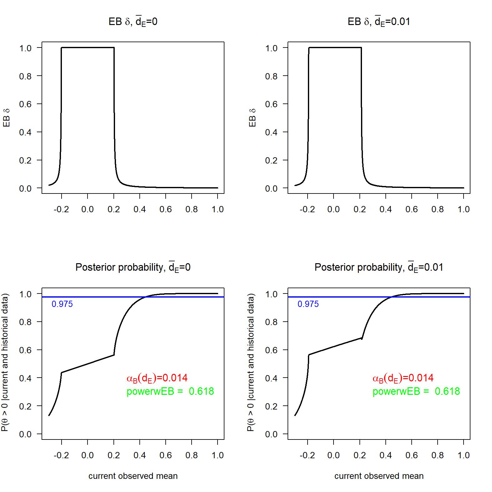
Figure S1: $\hat{\delta}(d;d_{E})$ (top) and the posterior probability $\textrm{P}(\theta>\theta_{0}\,|\,D=d;D_{E}=d_{E})$ (bottom) for varying current data mean $\bar{d}$ for $\bar{d}_{E}=0$ (left) and $\bar{d}_{E}=0.01$ (right).

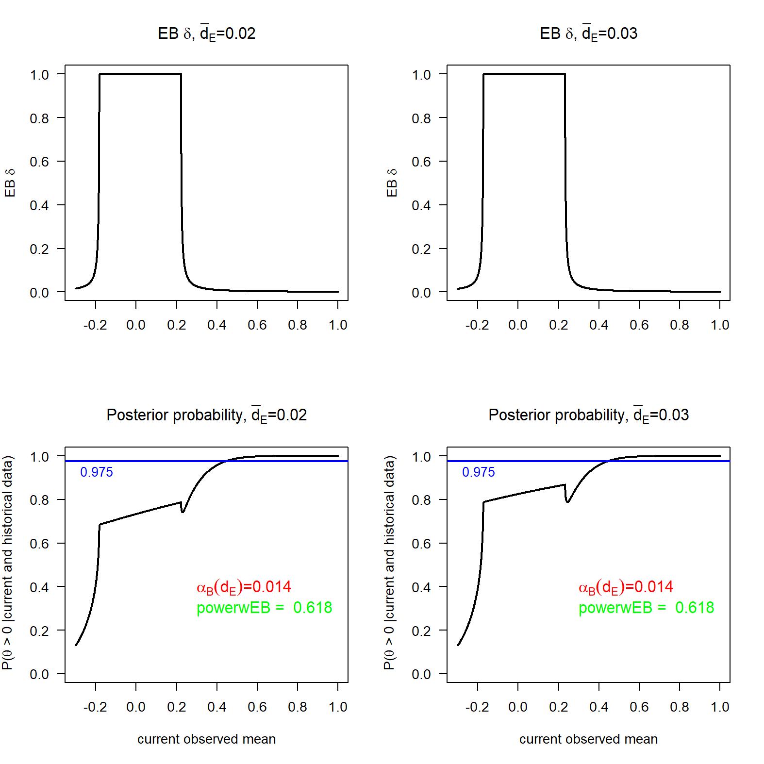
Figure S2: $\hat{\delta}(d;d_{E})$ (top) and the posterior probability $\textrm{P}(\theta>\theta_{0}\,|\,D=d;D_{E}=d_{E})$ (bottom) for varying current data mean $\bar{d}$ for $\bar{d}_{E}=0.02$ (left) and $\bar{d}_{E}=0.03$ (right).

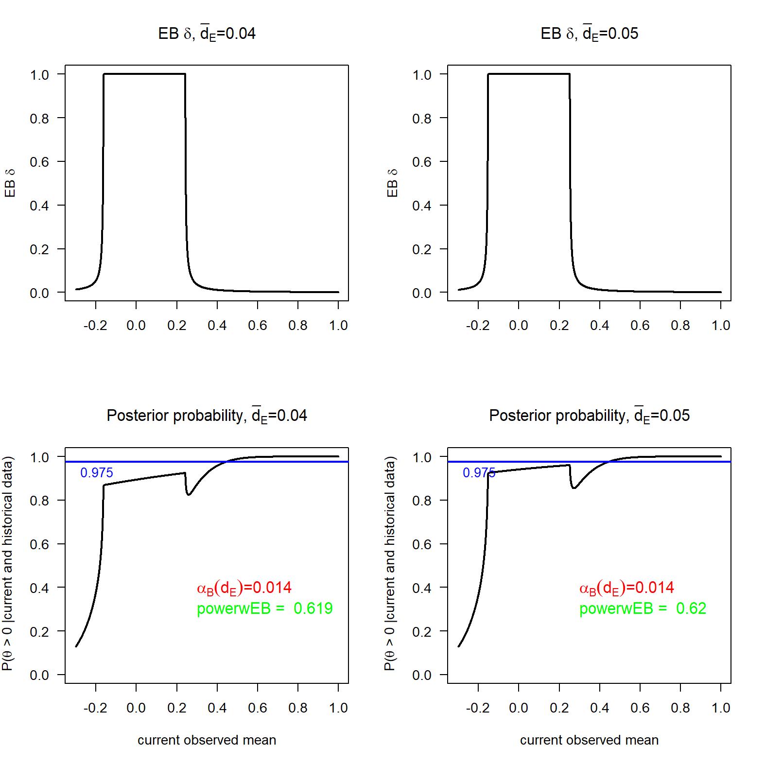
Figure S3: $\hat{\delta}(d;d_{E})$ (top) and the posterior probability $\textrm{P}(\theta>\theta_{0}\,|\,D=d;D_{E}=d_{E})$ (bottom) for varying current data mean $\bar{d}$ for $\bar{d}_{E}=0.04$ (left) and $\bar{d}_{E}=0.05$ (right).

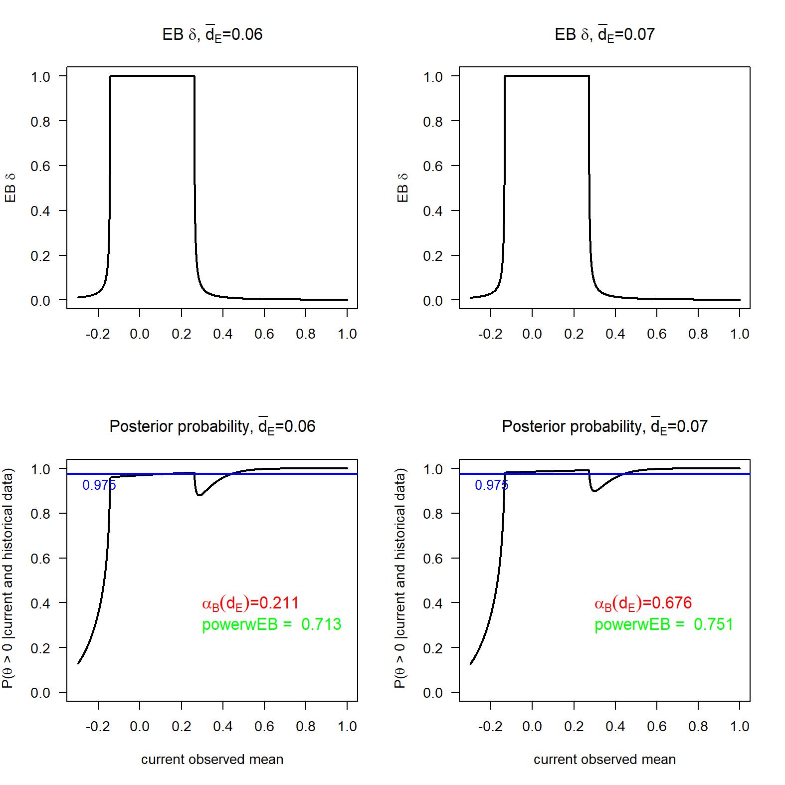
Figure S4: $\hat{\delta}(d;d_{E})$ (top) and the posterior probability $\textrm{P}(\theta>\theta_{0}\,|\,D=d;D_{E}=d_{E})$ (bottom) for varying current data mean $\bar{d}$ for $\bar{d}_{E}=0.06$ (left) and $\bar{d}_{E}=0.07$ (right).

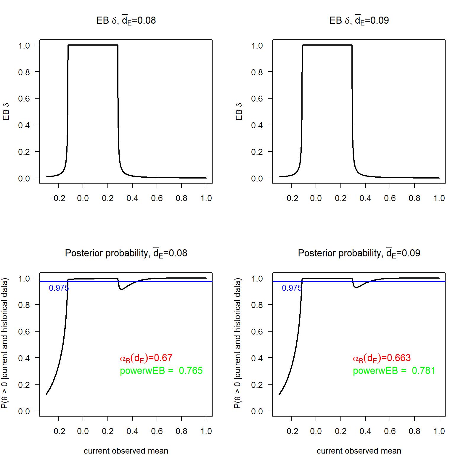
Figure S5: $\hat{\delta}(d;d_{E})$ (top) and the posterior probability $\textrm{P}(\theta>\theta_{0}\,|\,D=d;D_{E}=d_{E})$ (bottom) for varying current data mean $\bar{d}$ for $\bar{d}_{E}=0.08$ (left) and $\bar{d}_{E}=0.09$ (right).

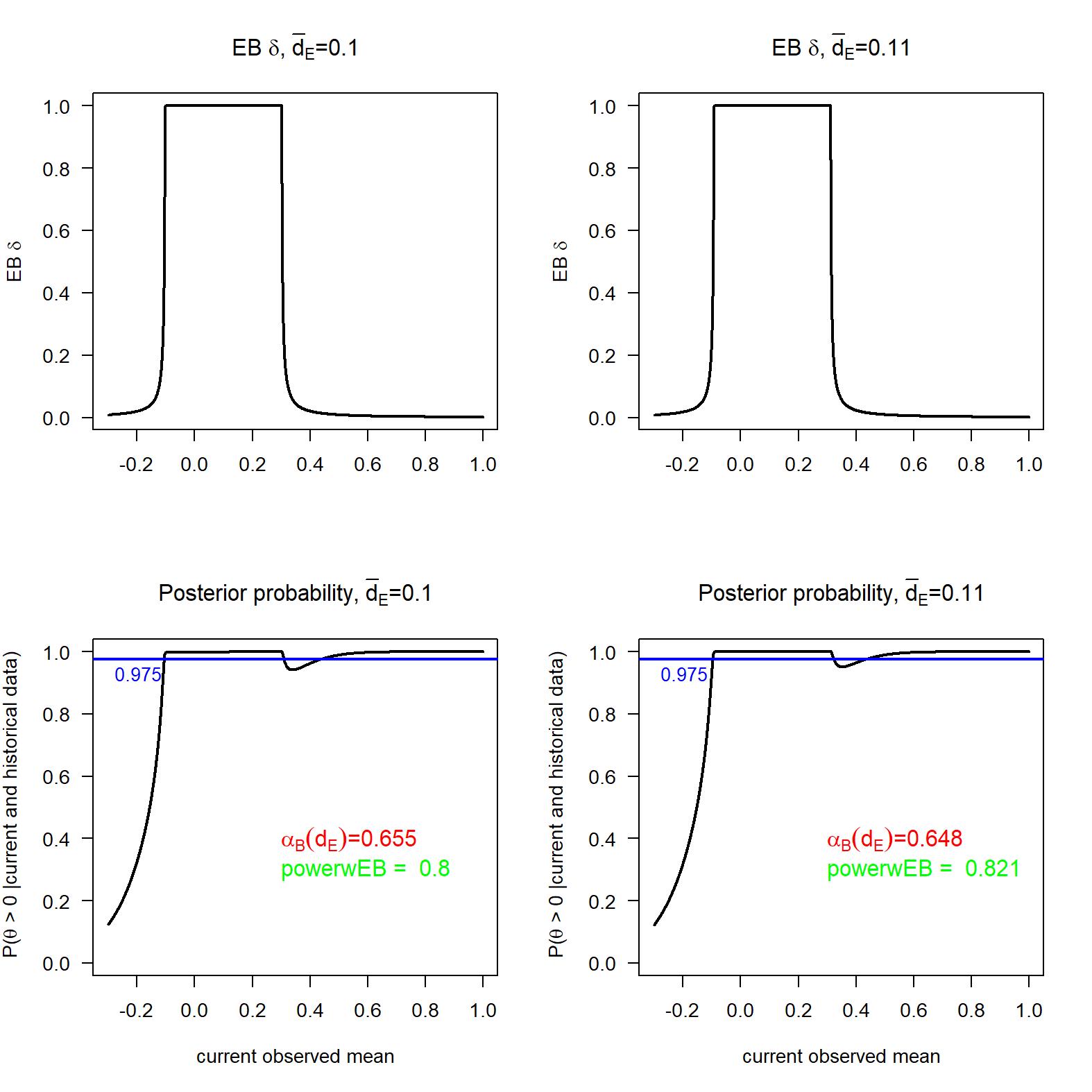
Figure S6: $\hat{\delta}(d;d_{E})$ (top) and the posterior probability $\textrm{P}(\theta>\theta_{0}\,|\,D=d;D_{E}=d_{E})$ (bottom) for varying current data mean $\bar{d}$ for $\bar{d}_{E}=0.10$ (left) and $\bar{d}_{E}=0.11$ (right).

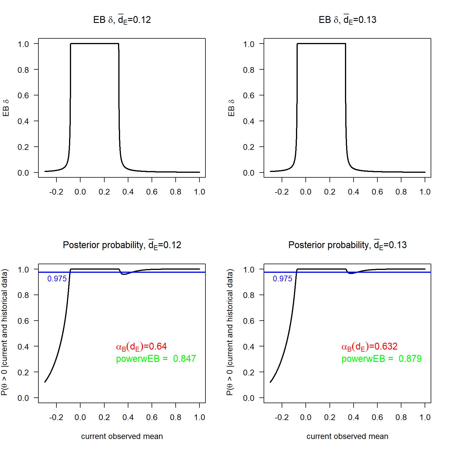
Figure S7: $\hat{\delta}(d;d_{E})$ (top) and the posterior probability $\textrm{P}(\theta>\theta_{0}\,|\,D=d;D_{E}=d_{E})$ (bottom) for varying current data mean $\bar{d}$ for $\bar{d}_{E}=0.12$ (left) and $\bar{d}_{E}=0.13$ (right).

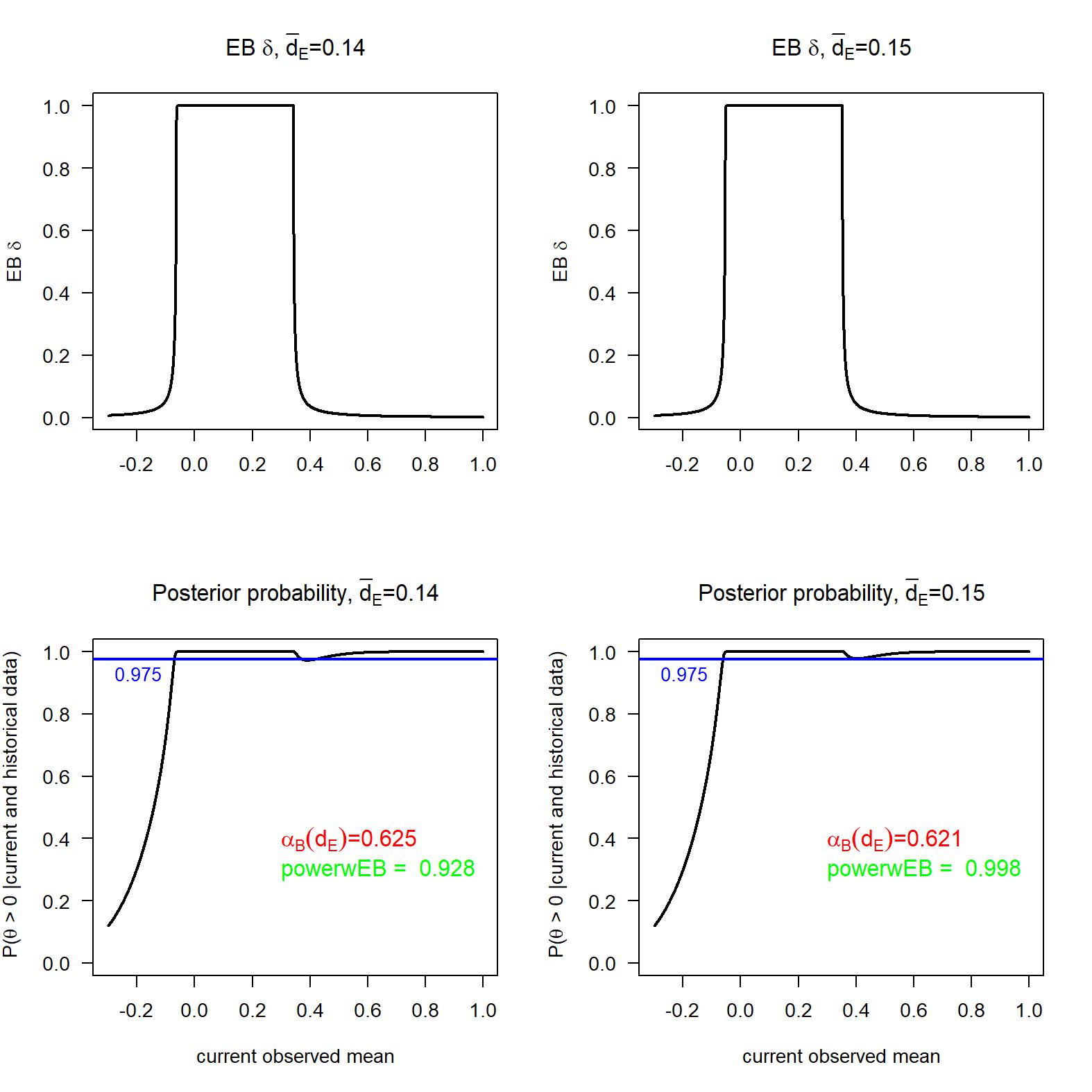
Figure S8: $\hat{\delta}(d;d_{E})$ (top) and the posterior probability $\textrm{P}(\theta>\theta_{0}\,|\,D=d;D_{E}=d_{E})$ (bottom) for varying current data mean $\bar{d}$ for $\bar{d}_{E}=0.14$ (left) and $\bar{d}_{E}=0.15$ (right).

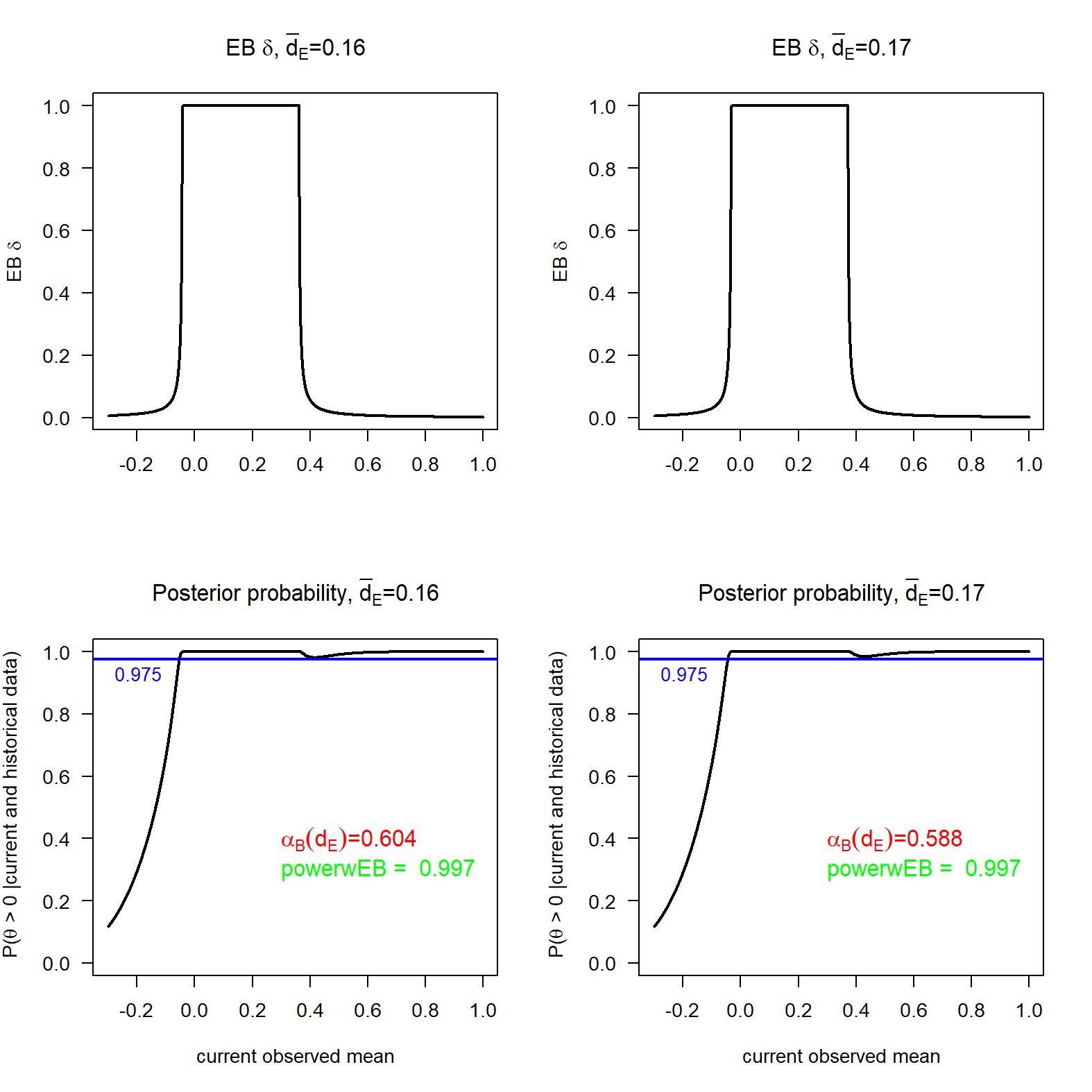
Figure S9: $\hat{\delta}(d;d_{E})$ (top) and the posterior probability $\textrm{P}(\theta>\theta_{0}\,|\,D=d;D_{E}=d_{E})$ (bottom) for varying current data mean $\bar{d}$ for $\bar{d}_{E}=0.16$ (left) and $\bar{d}_{E}=0.17$ (right).

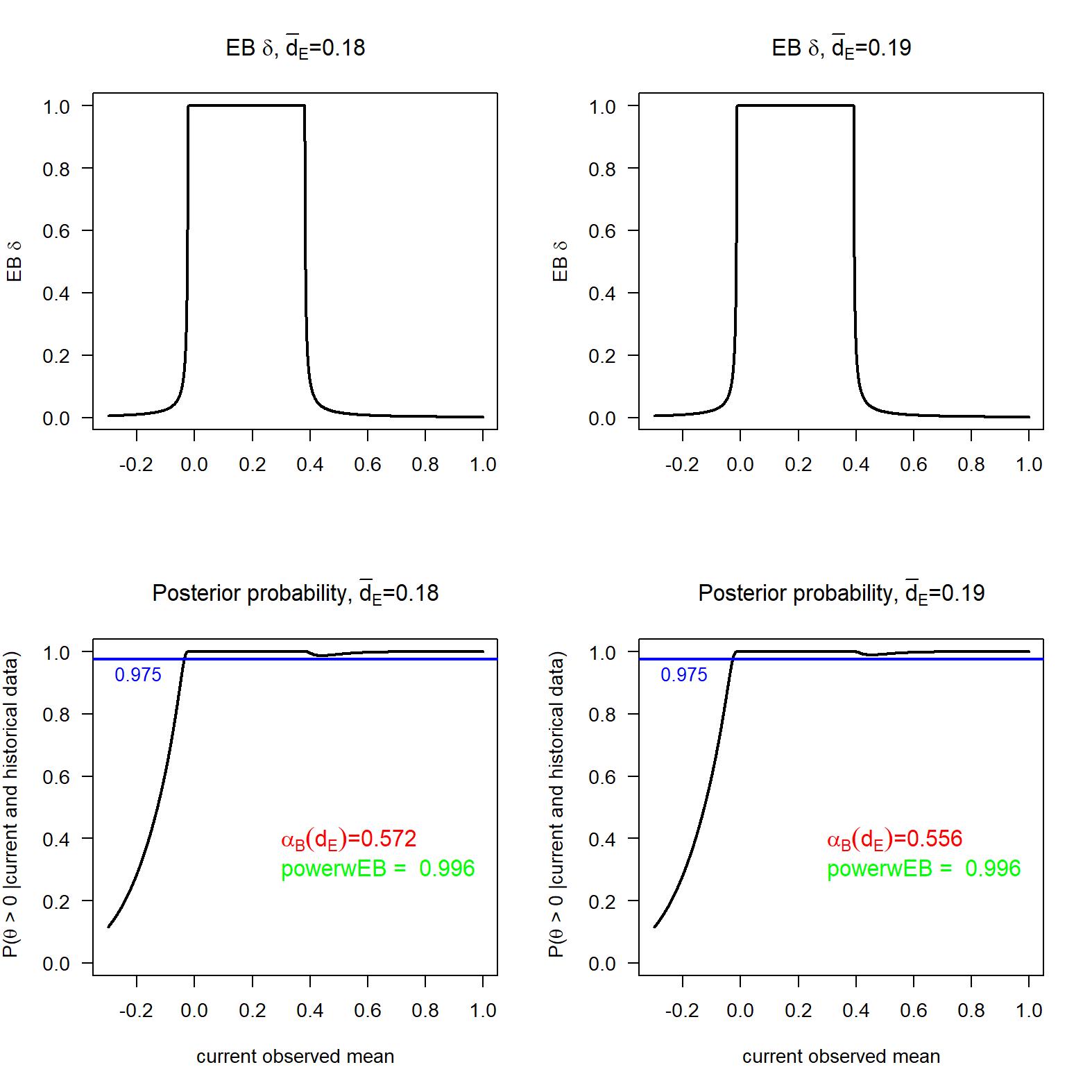
Figure S10: $\hat{\delta}(d;d_{E})$ (top) and the posterior probability $\textrm{P}(\theta>\theta_{0}\,|\,D=d;D_{E}=d_{E})$ (bottom) for varying current data mean $\bar{d}$ for $\bar{d}_{E}=0.18$ (left) and $\bar{d}_{E}=0.19$ (right).

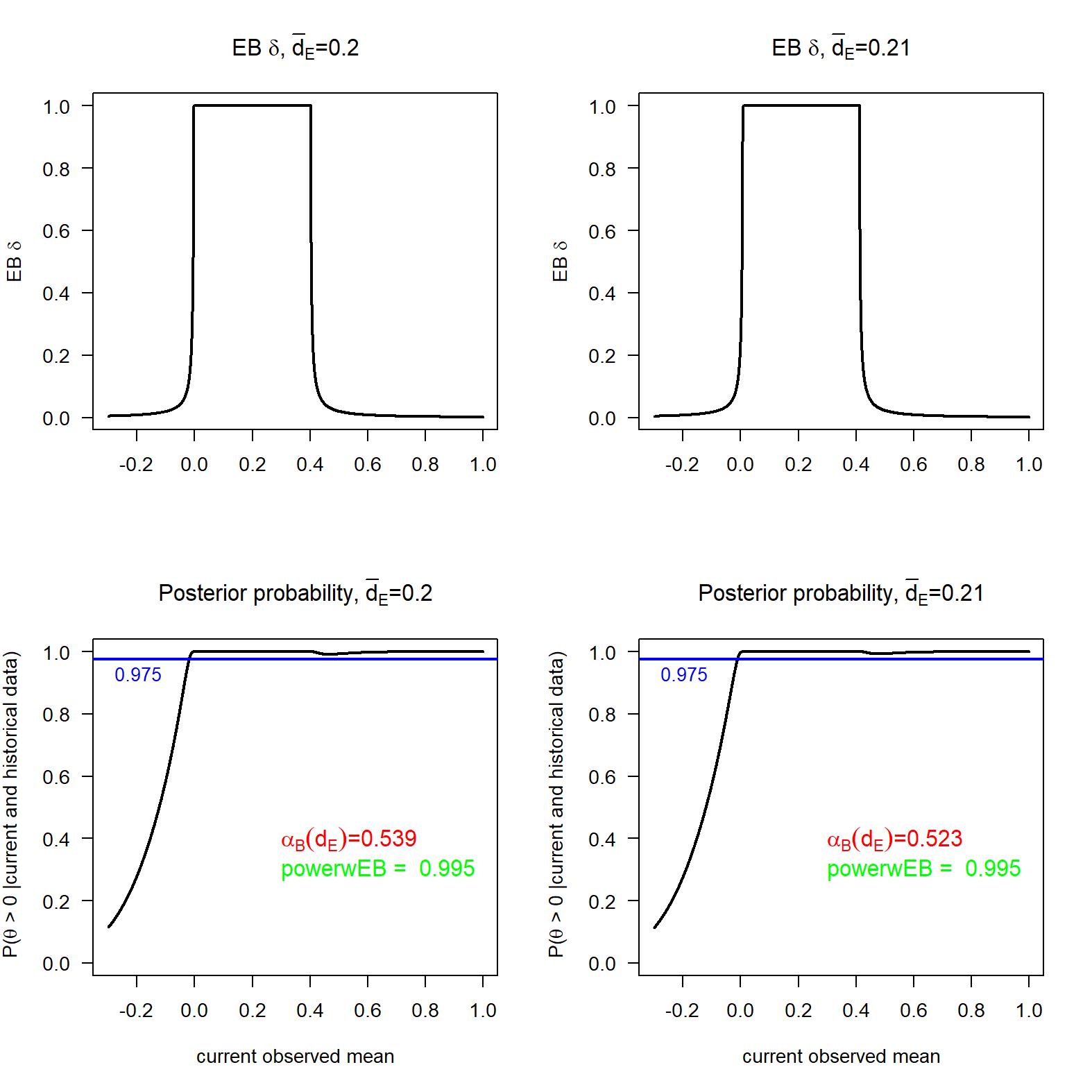
Figure S11: $\hat{\delta}(d;d_{E})$ (top) and the posterior probability $\textrm{P}(\theta>\theta_{0}\,|\,D=d;D_{E}=d_{E})$ (bottom) for varying current data mean $\bar{d}$ for $\bar{d}_{E}=0.20$ (left) and $\bar{d}_{E}=0.21$ (right).