Parameter estimation in generalised logistic model with application to DIF detection

Abstract

This paper proposes innovations to parameter estimation in a generalised logistic regression model in the context of detecting differential item functioning in multi-item measurements. The two newly proposed iterative algorithms are compared with existing methods in a simulation study, and their use is demonstrated in a real data example. Additionally the study examines software implementation including specification of initial values for iterative algorithms, and asymptotic properties with estimation of standard errors. Overall, the proposed methods gave comparable results to existing ones and were superior in some scenarios.

1 Introduction

Logistic regression <e.g.,¿agresti2010analysis is one of the most popular tools for describing item functioning in multi-item measurements. This method might be used in various contexts, including educational measurements, admission tests, cognitive assessments, and other health-related inventories. However, its broad applications are not limited to behavioural disciplines. In the context of psychometrics, logistic regression can be seen as a score-based counterpart to the 2 Parameter Logistic (PL) Item Response Theory (IRT) model Birnbaum (1968), since in contrast to this class of generalised linear mixed effect models, this method uses an observed estimate of the underlying latent trait.

Furthermore, logistic regression has become a widely used method for identifying between-group differences on item level when responding to multi-item measurements Swaminathan  Rogers (1990). The phenomenon which is known as Differential Item Functioning (DIF) indicates whether responses to an item vary for respondents with the same level of an underlying latent trait but from different social groups (e.g., defined by gender, age, or socio-economic status). In this vein, DIF detection is essential for a deeper understanding of group differences, for assessing effectiveness of various treatments, or for uncovering potential unfairness in educational tests. Beyond the logistic regression, various psychometrics and statistical methods have been proposed for an important task of DIF identification which are still being studied extensively Schneider . (2021); Schauberger  Tutz (2016); Paek  Fukuhara (2015); Suh  Bolt (2011).

A natural extension of the logistic regression model to describe item functioning is a generalised logistic regression model, which may account for the possibility that an item can be correctly answered or endorsed without the necessary knowledge or trait. In this case, the model is extended by including a parameter defining a lower asymptote of the probability curve, which may be larger than zero. Similarly, the model can consider the possibility that an item is incorrectly answered or opposed by a respondent with a high level of a certain trait due to issues such as inattention or lack of time. That is, the model includes an upper asymptote of the probability curve which may be lower than one. Analogous to the logistic regression model’s being a counterpart to the 2PL IRT model, generalised logistic regression models can be seen as score-based counterparts to 3–4PL IRT models Birnbaum (1968); Barton  Lord (1981).

The estimation in the logistic regression model is a straightforward procedure, but including additional parameters in this model makes it more statistically and computationally challenging and demanding. Therefore, this article examines innovations in the item parameter estimation for the generalised logistic regression model in the context of DIF detection. This work proposes novel iterative algorithms and compares the newly proposed methods to existing ones in a simulation study.

To begin, Section 2 introduces generalised logistic regression models, examining the estimation techniques. This section provides a detailed description of two existing methods for parameter estimation (Nonlinear Least Squares (NLS) and the Maximum Likelihood (ML) method) and their application to fitting a generalised logistic regression model. Furthermore, this study proposes a novel implementation of the Expectation-Maximisation (EM) algorithm and a new approach based on a Parametric Link Function (PLF). Additionally, this section provides asymptotic properties of the estimates, an estimation of standard errors, and a software implementation including a specification of starting values in iterative algorithms. Subsequently, Section 3 describes the design and results of the simulation study. To illustrate differences and challenges between the existing and newly proposed methods in practice, this work provides a real data analysis of anxiety measure in Section 4. Finally, Section 5 contains the discussion and conclusion remarks.

2 Methodology

2.1 Generalised logistic model for item functioning

Generalised logistic regression models are extensions of the logistic regression model which may account for the possibility of guessing or inattention when answering an item. The simple 4PL model describes functioning of the item $i$, meaning the probability of endorsing item $i$ by respondent $p$, by introducing four parameters:

$$\pi_{pi}=\mathrm{P}(Y_{pi}=1|X_{p})=c_{i}+(d_{i}-c_{i})\ \frac{\exp(b_{i0}+b_{i1}X_{p})}{1+\exp(b_{i0}+b_{i1}X_{p})},$$ (1)

with $X_{p}$ being an observed trait of respondent $p$.

Parameter interpretation.

All four parameters have an intuitive interpretation: The parameters $c_{i}$ and $d_{i}$ are the upper and lower asymptotes of the probability sigmoid function $\pi_{pi}(x)$ since

$$\lim_{x\to-\infty}\pi_{pi}(x)=c_{i}\quad\text{and}\quad\lim_{x\to\infty}\pi_{pi}(x)=d_{i},$$

where $c_{i}\in[0,1],d_{i}\in[0,1]$ and $c_{i}<d_{i}$ if $b_{i1}>0$ and $c_{i}>d_{i}$ otherwise. Evidently, with $c_{i}=0$ and $d_{i}=1$, this model recovers a standard logistic regression for item $i$.

In the context of psychological and health-related assessments, the asymptotes $c_{i}$ and $d_{i}$ may represent reluctance to admit difficulties due to social norms. In educational testing, parameter $c_{i}$ can be interpreted as the probability that the respondents guessed the correct answer without possessing the necessary knowledge $X_{p}$, also known as a pseudo-guessing parameter. On the other hand, $1-d_{i}$ can be viewed as the probability that respondents were inattentive while their knowledge $X_{p}$ was sufficient Hladká  Martinková (2020) or as a lapse-rate Kingdom  Prins (2016). Next, parameter $b_{i0}$ is a shift parameter, a midpoint between two asymptotes $c_{i}$ and $d_{i}$ related to the difficulty or easiness of item $i$. Finally, parameter $b_{i1}$ is linked to a slope of the sigmoid curve $\pi_{pi}(x)$, which is also called a discrimination of the respective item.

Adding covariates, group-specific 4PL model.

The simple model (1) can be further extended by incorporating additional respondents’ characteristics. That is, instead of using a single variable $X_{p}$ to describe item functioning, a vector of covariates $\boldsymbol{X}_{p}=(1,X_{p1},\dots,X_{pk})$, $p=1,\dots,n$, is involved, including the original observed trait and an intercept term. This process produces extra parameters $\boldsymbol{b}_{i}=(b_{i0},\dots,b_{ik})$. Beyond this, even asymptotes may depend on respondents’ characteristics $\boldsymbol{Z}_{p}=(1,Z_{p1},\dots,Z_{pj})$, $p=1,\dots,n$, which are not necessarily the same as $\boldsymbol{X}_{p}$. This, the general covariate-specific 4PL model is of form

$$\pi_{pi}=\mathrm{P}(Y_{pi}=1|\boldsymbol{X}_{p},\boldsymbol{Z}_{p})=\boldsymbol{Z}_{p}\boldsymbol{c}_{i}+(\boldsymbol{Z}_{p}\boldsymbol{d}_{i}-\boldsymbol{Z}_{p}\boldsymbol{c}_{i})\ \frac{\exp(\boldsymbol{X}_{p}\boldsymbol{b}_{i})}{1+\exp(\boldsymbol{X}_{p}\boldsymbol{b}_{i})},$$ (2)

where $\boldsymbol{c}_{i}=(c_{i0},\dots,c_{ij})$ and $\boldsymbol{d}_{i}=(d_{i0},\dots,d_{ij})$ are related asymptote parameters for item $i$.

As a special case of the covariate-specific 4PL model (2), an additional single binary covariate $G_{p}$ might be considered. This grouping variable describes a respondent’s membership to a social group ($G_{p}=0$ for the reference group and $G_{p}=1$ for the focal group). In other words, this special case assumes $\boldsymbol{X}_{p}=(1,X_{p},G_{p})$ and $\boldsymbol{Z}_{p}=(1,G_{p})$, which reduces the covariate-specific 4PL model (2) to a group-specific form:

$$\begin{split}\pi_{pi}=\ &\mathrm{P}(Y_{pi}=\ 1|X_{p},G_{p})=c_{i}+c_{i\text{DIF}}G_{p}\\ &+(d_{i}-d_{i\text{DIF}}G_{p}-c_{i}-c_{i\text{DIF}}G_{p})\ \frac{\exp(b_{i0}+b_{i1}X_{p}+b_{i2}G_{p}+b_{i3}G_{p}X_{p})}{1+\exp(b_{i0}+b_{i1}X_{p}+b_{i2}G_{p}+b_{i3}G_{p}X_{p})}.\end{split}$$ (3)

The group-specific 4PL model (3) can be used for testing between-group differences on the item level with a DIF analysis Hladká  Martinková (2020).

In this model, $X_{p}$ is an observed variable describing the measured trait of the respondent, such as anxiety, fatigue, quality of life, or math ability, here called the matching criterion. In the context of the logistic regression method for DIF detection, the total test score is typically used as the matching criterion Swaminathan  Rogers (1990). Other options for the matching criterion include a pre-test score, a score on another test measuring the same construct, or an estimate of the latent trait provided by an IRT model.

2.2 Estimation of item parameters

Numerous algorithms are available to estimate item parameters in the covariate-specific 4PL model (2). First, this section describes two methods, which may be directly implemented in the existing software: The NLS method and the ML method. This study discusses the asymptotic properties of the estimates. Next, the study introduces two newly proposed iterative algorithms, which might improve implementation of the computationally demanding ML method: The EM algorithm inspired by the work of dinse2011algorithm and an iterative algorithm based on PLF.

2.2.1 Nonlinear least squares

The parameter estimates of the covariate-specific 4PL model (2) can be determined using the NLS method Dennis . (1981), which is based on minimisation of the Residual Sum of Squares (RSS) of item $i$ with respect to item parameters $(\boldsymbol{b}_{i},\boldsymbol{c}_{i},\boldsymbol{d}_{i})$:

$$\text{RSS}_{i}(\boldsymbol{b}_{i},\boldsymbol{c}_{i},\boldsymbol{d}_{i})=\sum_{p=1}^{n}\left[Y_{pi}-\pi_{pi}\right]^{2}=\sum_{p=1}^{n}\left[Y_{pi}-\boldsymbol{Z}_{p}\boldsymbol{c}_{i}-(\boldsymbol{Z}_{p}\boldsymbol{d}_{i}-\boldsymbol{Z}_{p}\boldsymbol{c}_{i})\frac{\exp(\boldsymbol{X}_{p}\boldsymbol{b}_{i})}{1+\exp(\boldsymbol{X}_{p}\boldsymbol{b}_{i})}\right]^{2},$$ (4)

where $n$ is a number of respondents. Since the criterion function $\text{RSS}_{i}(\boldsymbol{b}_{i},\boldsymbol{c}_{i},\boldsymbol{d}_{i})$ is continuously differentiable with respect to item parameters $(\boldsymbol{b}_{i},\boldsymbol{c}_{i},\boldsymbol{d}_{i})$, the minimiser can be obtained when the gradient is zero. Thus, the minimisation process involves a calculation of the first partial derivatives with respect to item parameters $(\boldsymbol{b}_{i},\boldsymbol{c}_{i},\boldsymbol{d}_{i})$ and finding a solution of relevant nonlinear estimating equations <e.g., ¿[Chapter 5]van2000asymptotic. Since $\boldsymbol{Z}_{p}\boldsymbol{c}_{i}$ and $\boldsymbol{Z}_{p}\boldsymbol{d}_{i}$ asymptotes represent probabilities, it is necessary to ensure that these expressions are kept in the interval of $[0,1]$ which is accomplished using numerical approaches.

The asymptotic properties of the NLS estimator, such as consistency and asymptotic distribution, can be derived under the classical set of regularity conditions <e.g.,¿[Theorems 5.41 and 5.42; see also Appendix A.1]van2000asymptotic. This study proposes a sandwich estimator (A1) which can be used as a natural estimate of the asymptotic variance of the NLS estimate.

2.2.2 Maximum likelihood

The second option for estimating item parameters in the covariate-specific 4PL model (2) is the ML method <e.g.,¿ren2019algorithm. Using a notation $\phi_{pi}=\frac{\exp(\boldsymbol{X}_{p}\boldsymbol{b}_{i})}{1+\exp(\boldsymbol{X}_{p}\boldsymbol{b}_{i})}$, the corresponding likelihood function for item $i$ has the following form:

$$L_{i}(\boldsymbol{b}_{i},\boldsymbol{c}_{i},\boldsymbol{d}_{i})=\prod_{p=1}^{n} \left[\boldsymbol{Z}_{p}\boldsymbol{c}_{i}+(\boldsymbol{Z}_{p}\boldsymbol{d}_{i}-\boldsymbol{Z}_{p}\boldsymbol{c}_{i})\phi_{pi}\right]^{Y_{pi}}\left[1-\boldsymbol{Z}_{p}\boldsymbol{c}_{i}-(\boldsymbol{Z}_{p}\boldsymbol{d}_{i}-\boldsymbol{Z}_{p}\boldsymbol{c}_{i})\phi_{pi}\right]^{1-Y_{pi}},$$

and the log-likelihood function is then given by

$$l_{i}(\boldsymbol{b}_{i},\boldsymbol{c}_{i},\boldsymbol{d}_{i})=\sum_{p=1}^{n} \left\{Y_{pi}\log(\boldsymbol{Z}_{p}\boldsymbol{c}_{i}+(\boldsymbol{Z}_{p}\boldsymbol{d}_{i}-\boldsymbol{Z}_{p}\boldsymbol{c}_{i})\phi_{pi})\right.$$

$$\ \left.+\ (1-Y_{pi})\log(1-\boldsymbol{Z}_{p}\boldsymbol{c}_{i}-(\boldsymbol{Z}_{p}\boldsymbol{d}_{i}-\boldsymbol{Z}_{p}\boldsymbol{c}_{i})\phi_{pi})\right\}.$$

The parameter estimates are obtained by a maximisation of the log-likelihood function. Thus this study proceeds similarly to the logistic regression model, except for a larger dimension of the parametric space. To find the maximiser of the log-likelihood function $l_{i}(\boldsymbol{b}_{i},\boldsymbol{c}_{i},\boldsymbol{d}_{i})$, the first partial derivatives are set to zero and these so-called likelihood equations must be solved. However, the solution of a system of the nonlinear equations cannot be derived algebraically and needs to be numerically estimated using a suitable iterative process.

Using van der Vaart’s 1998 Theorems 5.41 and 5.42, consistency and asymptotic normality can be shown for the ML estimator, see Appendix A.2. Additionally, the estimate of the asymptotic variance of the item parameters is an inverse of the observed information matrix (A2).

2.2.3 EM algorithm

The ML method may be computationally demanding and iterative algorithms might help in those situations. Inspired by the work of dinse2011algorithm, this study adopts a version of the EM algorithm Dempster . (1977) for parameter estimation in the covariate-specific 4PL model (2).

Next, the original problem can be reformulated using latent variables which describe hypothetical responses status of test-takers Dinse (2011). In this study’s setting, the work considers four mutually exclusive latent variables ($W_{pi1}$, $W_{pi2}$, $W_{pi3}$, $W_{pi4}$), where variable $W_{pij}=1$ indicates that respondent $p$ belongs in the category $j=1,\dots,4$ for an item $i$, whereas $W_{pij}=0$ indicates that respondent does not belong in this category.

In the context of educational, psychological, health-related, or other types of multi-item measurement, the four categories can be interpreted as follows: Categories 1 and 2 indicate whether a respondent who responded correctly to item $i$ or endorsed it (i.e., $Y_{pi}=1$) was determined to do so ($W_{pi1}=1$, e.g., the respondent guessed correct answer while their knowledge or ability was insufficient) or not ($W_{pi2}=1$, e.g., had a sufficient knowledge or ability to answer correctly and did not guessed). On the other hand, Categories 3 and 4 indicate whether the respondent who did not respond correctly or did not endorse the item (i.e., $Y_{pi}=0$) was prone to do so ($W_{pi3}=1$, e.g., did not have sufficient knowledge or ability) or not ($W_{pi4}=1$, e.g., incorrectly answered due to another reason such as inattention or lack of time). Thus, the observed indicator $Y_{pi}$ and its complement $1-Y_{pi}$ could be rewritten as $Y_{pi}=W_{pi1}+W_{pi2}$ and $1-Y_{pi}=W_{pi3}+W_{pi4}$ (Figure 1).

Figure 1: Latent variables for EM algorithm

Let $\boldsymbol{Z}_{p}\boldsymbol{c}_{i}$ be the regressor-based probability that the respondent was determined to respond to item $i$ correctly or endorse it (Category 1), and let $\boldsymbol{Z}_{p}\boldsymbol{d}_{i}$ be the regressor-based probability of the respondent not prone to respond correctly or endorse item $i$ (Categories 1–3). Then $\boldsymbol{Z}_{p}\boldsymbol{d}_{i}-\boldsymbol{Z}_{p}\boldsymbol{c}_{i}$ gives the regressor-based probability that the respondent was not determined but prone to (Categories 2 and 3). Further, we denote $\phi_{pi}$ and $1-\phi_{pi}$ – the probabilities to answer given item correctly (Category 2) and incorrectly (Category 3), respectively, depending on the regressors $\boldsymbol{X}_{p}$. Finally, the probability that the respondent did not respond correctly and was not prone to do so is given by $1-(\boldsymbol{Z}_{p}\boldsymbol{d}_{i}-\boldsymbol{Z}_{p}\boldsymbol{c}_{i})-\boldsymbol{Z}_{p}\boldsymbol{c}_{i}=1-\boldsymbol{Z}_{p}\boldsymbol{d}_{i}$ (Category 4). In summary, the expected values of the latent variables are then given by the following terms

$$\boldsymbol{Z}_{p}\boldsymbol{c}_{i},\ \ (\boldsymbol{Z}_{p}\boldsymbol{d}_{i}-\boldsymbol{Z}_{p}\boldsymbol{c}_{i})\phi_{pi},\ \ (\boldsymbol{Z}_{p}\boldsymbol{d}_{i}-\boldsymbol{Z}_{p}\boldsymbol{c}_{i})(1-\phi_{pi}),\ \ 1-\boldsymbol{Z}_{p}\boldsymbol{d}_{i},$$

and the probability of correct response or endorsement is given by

$$\mathrm{P}(Y_{pi}=1|\boldsymbol{X}_{p})= \ \mathrm{P}(W_{pi1}+W_{pi2}=1|\boldsymbol{X}_{p})=\mathrm{P}(W_{pi1}=1|\boldsymbol{X}_{p})+\mathrm{P}(W_{pi2}=1|\boldsymbol{X}_{p})$$

$$= \ \boldsymbol{Z}_{p}\boldsymbol{c}_{i}+(\boldsymbol{Z}_{p}\boldsymbol{d}_{i}-\boldsymbol{Z}_{p}\boldsymbol{c}_{i})\phi_{pi},$$

which under the logistic model $\phi_{pi}=\frac{\exp(\boldsymbol{X}_{p}\boldsymbol{b}_{i})}{1+\exp(\boldsymbol{X}_{p}\boldsymbol{b}_{i})}$ produces the covariate-specific 4PL model (2).

Using the setting of the latent variables, the corresponding log-likelihood function for item $i$ takes the following form:

$$l_{i}^{\text{EM}}= \sum_{p=1}^{n}\left[W_{pi2}\log\left(\phi_{pi}\right)+W_{pi3}\log\left(1-\phi_{pi}\right)\right]$$

$$+\sum_{p=1}^{n}\left[W_{pi1}\log\left(\boldsymbol{Z}_{p}\boldsymbol{c}_{i}\right)+W_{pi4}\log\left(1-\boldsymbol{Z}_{p}\boldsymbol{d}_{i}\right)+\ \left(W_{pi2}+W_{pi3}\right)\log\left(\boldsymbol{Z}_{p}\boldsymbol{d}_{i}-\boldsymbol{Z}_{p}\boldsymbol{c}_{i}\right)\right]$$

$$= \ l_{i1}^{\text{EM}}+l_{i2}^{\text{EM}}.$$

The log-likelihood function $l_{i1}^{\text{EM}}$ includes only parameters $\boldsymbol{b}_{i}$ and regressors $\boldsymbol{X}_{p}$, whereas the log-likelihood function $l_{i2}^{\text{EM}}$ incorporates only parameters related to the asymptotes of the sigmoid function and includes only regressors $\boldsymbol{Z}_{p}$. Notably, the log-likelihood function $l_{i1}^{\text{EM}}$ has a form of the log-likelihood function for the logistic regression. However, in contrast to the logistic regression model, in this setting it does not necessary hold that $W_{pi2}+W_{pi3}=1$ since the correct answer could be guessed or the respondent could be inattentive, producing $W_{pi2}+W_{pi3}=0$. The log-likelihood function $l_{i2}^{\text{EM}}$ takes the form of the log-likelihood for multinomial data with one trial and with the regressor-based probabilities $\boldsymbol{Z}_{p}\boldsymbol{c}_{i}$, $\boldsymbol{Z}_{p}\boldsymbol{d}_{i}-\boldsymbol{Z}_{p}\boldsymbol{c}_{i}$, and $1-\boldsymbol{Z}_{p}\boldsymbol{d}_{i}$.

The EM algorithm estimates item parameters in two steps – expectation and maximisation. These two steps are repeated until the convergence criterion is met, such as until the change in log-likelihood is lower than a predefined value.

Expectation.

At the E-step, conditionally on the item responses $Y_{pi}$ and the current parameter estimate $(\widehat{\boldsymbol{b}}_{i},\widehat{\boldsymbol{c}}_{i},\widehat{\boldsymbol{d}}_{i})$, the estimates of latent variables are calculated as their expected values:

$$\begin{aligned} \widehat{W}_{pi1}=&\ \frac{\boldsymbol{Z}_{p}\widehat{\boldsymbol{c}}_{i}Y_{pi}}{\boldsymbol{Z}_{p}\widehat{\boldsymbol{c}}_{i}+(\boldsymbol{Z}_{p}\widehat{\boldsymbol{d}}_{i}-\boldsymbol{Z}_{p}\widehat{\boldsymbol{c}}_{i})\widehat{\phi}_{pi}},\ \ \ &\widehat{W}_{pi2}=&\ Y_{pi}-\widehat{W}_{pi1},\\ \widehat{W}_{pi4}=&\ \frac{\left(1-\boldsymbol{Z}_{p}\widehat{\boldsymbol{d}}_{i}\right)\left(1-Y_{pi}\right)}{1-\widehat{\boldsymbol{Z}_{p}\boldsymbol{c}}_{i}-(\boldsymbol{Z}_{p}\widehat{\boldsymbol{d}}_{i}-\boldsymbol{Z}_{p}\widehat{\boldsymbol{c}}_{i})\widehat{\phi}_{pi}},\ \ \ &\widehat{W}_{pi3}=&\ 1-Y_{pi}-\widehat{W}_{pi4}.\end{aligned}$$ (5)

Maximisation.

At the M-step, conditionally on the current estimates of the latent variables $\widehat{W}_{pi2}$ and $\widehat{W}_{pi3}$, the estimates of parameters $\boldsymbol{b}_{i}$ maximise the log-likelihood function $l_{i1}^{\text{EM}}$. The estimates $\widehat{\boldsymbol{c}}_{i}$ and $\widehat{\boldsymbol{d}}_{i}$ are given by a maximisation of the log-likelihood function $l_{i2}^{\text{EM}}$ conditionally on current estimates of the latent variables $\widehat{W}_{pi1}$, $\widehat{W}_{pi2}$, $\widehat{W}_{pi3}$, and $\widehat{W}_{pi4}$.

The EM algorithm is designed to gain the ML estimates of the item parameters, so estimates have the same asymptotic properties as described above.

2.2.4 Parametric link function

In this study’s setting, the covariate-specific 4PL model (2) can be viewed as a generalised linear model with a known PLF

$$g(\mu_{pi};\boldsymbol{c}_{i},\boldsymbol{d}_{i})=\log\left(\frac{\mu_{pi}-\boldsymbol{Z}_{p}\boldsymbol{c}_{i}}{\boldsymbol{Z}_{p}\boldsymbol{d}_{i}-\mu_{pi}}\right),$$ (6)

where the parameters $\boldsymbol{c}_{i}$ and $\boldsymbol{d}_{i}$ are unknown and may depend on regressors $\boldsymbol{Z}_{p}$. Subsequently, the mean function is determined by $\mu_{pi}=\pi_{pi}$ as given by (2) with a linear predictor $\boldsymbol{X}_{p}\boldsymbol{b}_{i}$.

Keeping this setting in mind, this study proposes a new two-stage algorithm to estimate item parameters using the PLF (6), which involves repeating two steps until the convergence criterion is fulfilled.

Step one.

First, conditionally on current estimates $\widehat{\boldsymbol{c}}_{i}$ and $\widehat{\boldsymbol{d}}_{i}$ of the PLF, the estimates of parameters $\boldsymbol{b}_{i}$ maximise the following log-likelihood function:

$$l_{i1}^{\text{PL}}(\boldsymbol{b}_{i}|\widehat{\boldsymbol{c}}_{i},\widehat{\boldsymbol{d}}_{i})=\sum_{p=1}^{n} \left\{Y_{pi}\log(\boldsymbol{Z}_{p}\widehat{\boldsymbol{c}}_{i}+(\boldsymbol{Z}_{p}\widehat{\boldsymbol{d}}_{i}-\boldsymbol{Z}_{p}\widehat{\boldsymbol{c}}_{i})\phi_{pi})\right.$$

$$\ \ \left.+\ (1-Y_{pi})\log(1-\boldsymbol{Z}_{p}\widehat{\boldsymbol{c}}_{i}-(\boldsymbol{Z}_{p}\widehat{\boldsymbol{d}}_{i}-\boldsymbol{Z}_{p}\widehat{\boldsymbol{c}}_{i})\phi_{pi})\right\}.$$

The log-likelihood function $l_{i1}^{\text{PL}}(\boldsymbol{b}_{i}|\widehat{\boldsymbol{c}}_{i},\widehat{\boldsymbol{d}}_{i})$ has a similar form to the log-likelihood function $l_{i}(\boldsymbol{b}_{i},\boldsymbol{c}_{i},\boldsymbol{d}_{i})$ using the ML method. However, the parameters $\boldsymbol{c}_{i}$ and $\boldsymbol{d}_{i}$ are here replaced by their current estimates, $\widehat{\boldsymbol{c}}_{i}$ and $\widehat{\boldsymbol{d}}_{i}$.

Step two.

Next, estimates $\widehat{\boldsymbol{c}}_{i}$ and $\widehat{\boldsymbol{d}}_{i}$ of the PLF (6) are calculated conditionally on the current estimates $\widehat{\boldsymbol{b}}_{i}$ as the arguments of the maxima of the following log-likelihood function

$$l_{i2}^{\text{PL}}(\boldsymbol{c}_{i},\boldsymbol{d}_{i}|\widehat{\boldsymbol{b}}_{i})=\sum_{p=1}^{n} \left\{Y_{pi}\log(\boldsymbol{Z}_{p}\boldsymbol{c}_{i}+(\boldsymbol{Z}_{p}\boldsymbol{d}_{i}-\boldsymbol{Z}_{p}\boldsymbol{c}_{i})\widehat{\phi}_{pi})\right.$$

$$\left.\ \ +\ (1-Y_{pi})\log(1-\boldsymbol{Z}_{p}\boldsymbol{c}_{i}-(\boldsymbol{Z}_{p}\boldsymbol{d}_{i}-\boldsymbol{Z}_{p}\boldsymbol{c}_{i})\widehat{\phi}_{pi})\right\}.$$

Again, the parameters $\boldsymbol{b}_{i}$ are replaced by their estimates $\widehat{\boldsymbol{b}}_{i}$, and $\phi_{pi}$ is thus replaced by $\widehat{\phi}_{pi}$.

In summary, the division into the two sets of parameters makes the algorithm based on PLF easy to implement in the R software and can take an advantage of its existing functions. Because the algorithm is designed to produce the ML estimates, their asymptotic properties are the same as described above.

2.3 Implementation and software

For all analyses, software R, version 4.1 R Core Team (2022) was used. The NLS method was implemented using the base nls() function and the "port" algorithm Gay (). The sandwich estimator (A1) of the asymptotic covariance matrix was computed using the calculus package Guidotti (2022). The ML estimation was performed with the base optim() function and the "L-BFGS-B" algorithm Byrd . (1995). The EM algorithm implements directly (5) in the expectation step using the base glm() function and the multinom() function from the nnet package Venables  Ripley (2002) in the maximisation step. Next, the step one of the newly proposed algorithm based on PLF is implemented with the base glm() function with the modified logit link, which includes asymptote parameters. The estimation of the asymptote parameters in the step two is conducted using the base optim() function. The maximum number of iterations was set to 2,000 for all four methods, and the convergence criterion was set to $10^{-6}$ when possible.

Initial values.

Starting values for item parameters were calculated as follows: The respondents were divided into three groups based upon tertiles of the matching criterion $X_{p}$. Next, the asymptote parameters were estimated: $c$ was computed as an empirical probability for those whose matching criterion was smaller than its average value in the first group defined by tertiles. The asymptote $d$ was calculated as an empirical probability of those whose matching criterion was greater than its average value in the last group defined by tertiles. The slope parameter $b_{1}$ was estimated as a difference between mean empirical probabilities of the last and the first group multiplied by 4. This difference is sometimes called upper-lower index. Finally, the intercept $b_{0}$ was calculated as follows: First, a centre point between the asymptotes was computed, and then we looked for the level of the matching criterion which would have corresponded to this empirical probability. Additionally, smoothing and corrections for variability of the matching criterion were applied.

3 Simulation study

A simulation study was performed to compare various procedures to estimate parameters in the generalised logistic regression model, including the NLS, the ML method, the EM algorithm, and the newly proposed algorithm based on PLF. Two models were considered – the simple 4PL model (1) and the group-specific 4PL model (3).

3.1 Simulation design

Data generation.

To generate data with the simple 4PL model (1), the following parameters were used: $b_{0}=0$, $b_{1}=1.5$, $c=0.25$, and $d=0.9$. In the case of the group-specific 4PL model (3), additionally $b_{2}=-1$, $b_{3}=0.5$, $c_{\text{DIF}}=-0.15$, and $d_{\text{DIF}}=0.1$ were considered. Next, the matching criterion $X_{p}$ was generated from the standard normal distribution for all respondents. Binary responses were generated from the Bernoulli distribution with the calculated probabilities based upon the chosen 4PL model, true parameters, and the matching criterion variable. The sample size was set to $n=500;1,000;2,500$; and $5,000$, i.e., $250$; $500$; $1,250$; and $2,500$ per group in the case of the group-specific 4PL model (3). Each scenario was replicated $1,000$ times.

Simulation evaluation.

To compare estimation methods, we first computed mean and median numbers of iteration runs and the convergence status of the methods, meaning the percentage of converged simulation runs; the percentage of runs which crashed (caused error when fitting, e.g., due to singularities); and the percentage of those which reached the maximum number of iterations without convergence. Next, we selected only those simulation runs for which all four estimation methods converged successfully and computed the mean parameter estimates, together with parametric confidence intervals. When confidence intervals for asymptote parameters exceeded their boundaries of 0 or 1, confidence intervals were truncated at the boundary value.

3.2 Simulation results

Convergence status.

All four methods had low percentages of iterations that crashed for all sample sizes in the simple 4PL model (1), but the rate was mildly increased in the group-specific 4PL model (3) for the NLS method (4.3%) and for the algorithm based on PLF (3.6%) when $n=500$. With the increasing sample size, convergence issues disappeared. The EM algorithm struggled to converge in a predefined number of iterations, especially for small sample sizes in both models. Additionally, the method based on PLF reached the maximum limit of 2,000 iterations only in a small percentage of simulation runs when smaller sample sizes were considered in the group-specific 4PL model (Table 1).

Number of iterations.

Furthermore, the methods differed in a number of iterations needed until the estimation process successfully ended. The EM algorithm yielded the largest mean and median numbers of iterations, which were somehow overestimated by simulation runs which did not finish without convergence (i.e., the maximum limit of 2,000 iterations was reached). The fewest iterations were needed for the NLS method. As expected, all the methods required fewer simulation runs when the simple 4PL model (1) was considered than in the group-specific 4PL model (3). Beyond this, the number of iterations was decreasing with the increasing sample size in both models for all the methods except the EM algorithm, where the number of iterations was not monotone (Table 1).

In the group-based model (3) with a sample size of $n=500$, some of the estimation procedures produced non-meaningful estimates of parameters $b_{0}$–$b_{3}$ (absolute value over 100) despite successful convergence. Those 11 simulations affected mean values significantly, so they were removed from a computation of the mean estimates and their confidence intervals for all four estimation methods. In those 11 simulations, non-meaningful estimates were received twice for the NLS, three times for the ML, eight times for the EM algorithm, and once for the PLF-based method.

Table 1: Convergence status and a number of iterations for the four estimation methods

Simple 4PL model (1) Group-specific 4PL model (3) Method Convergence status [%] Number of iterations Convergence status [%] Number of iterations Converged Crashed DNF Mean Median Converged Crashed DNF Mean Median $n=500$ NLS 99.60 0.40 0.00 10.11 9.00 95.70 4.30 0.00 14.36 12.00 MLE 99.60 0.40 0.00 22.99 22.00 99.90 0.10 0.00 90.63 80.00 EM 84.70 0.00 15.30 684.83 361.00 89.30 0.10 10.60 627.13 354.00 PLF 99.80 0.20 0.00 43.73 20.00 95.90 3.60 0.50 131.48 35.50 $n=1,000$ NLS 100.00 0.00 0.00 7.98 7.00 99.60 0.40 0.00 11.07 10.00 MLE 100.00 0.00 0.00 21.40 21.00 100.00 0.00 0.00 80.25 75.00 EM 83.70 0.00 16.30 744.01 437.00 88.20 0.00 11.80 769.27 542.00 PLF 100.00 0.00 0.00 31.13 18.00 99.30 0.60 0.10 76.85 27.00 $n=2,500$ NLS 99.90 0.10 0.00 5.90 6.00 99.90 0.10 0.00 7.58 7.00 MLE 99.90 0.10 0.00 19.98 19.00 100.00 0.00 0.00 73.01 72.00 EM 92.60 0.20 7.20 634.03 475.50 90.90 0.00 9.10 695.99 499.00 PLF 100.00 0.00 0.00 17.77 16.00 100.00 0.00 0.00 38.08 19.50 $n=5,000$ NLS 99.90 0.10 0.00 5.07 5.00 99.80 0.20 0.00 6.02 6.00 MLE 100.00 0.00 0.00 19.21 19.00 100.00 0.00 0.00 69.81 69.00 EM 95.60 0.00 4.40 588.82 477.50 92.60 0.00 7.40 808.35 647.50 PLF 100.00 0.00 0.00 15.40 15.00 100.00 0.00 0.00 26.07 16.00

x
Note. DNF = did not finish, NLS = nonlinear least squares, MLE = maximum likelihood estimation, EM = expectation-maximisation algorithm, PLF = algorithm based on parametric link function.

Parameter estimates.

In the simple 4PL model (1), the smallest biases in estimates of parameters $b_{0}$ and $b_{1}$ were gained by the PLF-based algorithm with the narrowest confidence intervals when smaller sample sizes were considered ($n=500$ or $n=1,000$). Additionally, in these scenarios, the NLS method yielded slightly more biased estimates with wider confidence intervals. The precision of the estimation improved for both parameters when the sample size increased in all four methods, whereas differences between estimation procedures narrowed. The precision of the estimates of the asymptote parameters $c$ and $d$ was similar for all four methods, while the differences between estimation approaches were small. The NLS and the EM algorithm provided slightly wider confidence intervals for a small sample size of $n=500$ (Figure 2, Table A1).

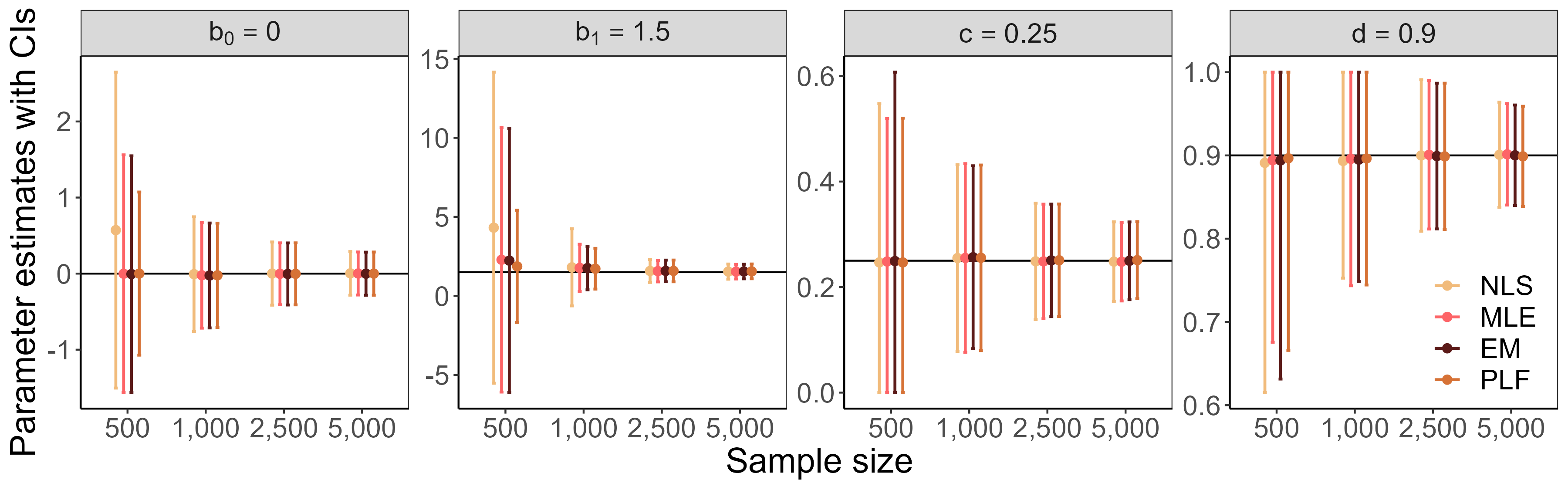
Figure 2: Mean estimated parameters in the simple 4PL model (1) with confidence intervals with respect to sample size; horizontal lines represent true values of parameters

In the group-specific 4PL model (3), the PLF-based algorithm yielded the least biased estimates of parameters $b_{0}$–$b_{3}$, especially for the smaller sample sizes. On the other hand, the NLS method produced the most biased estimates with somewhat wider confidence intervals in such scenarios. The ML method provided less biased estimates than the NLS, but accompanied with wider confidence intervals, even for a sample size of $n=1,000$. Similar to the simple 4PL model (1), the differences in the precision of the parameter estimates were narrowing with the increasing sample size, and all four estimation approaches gave estimates close to the true values of the item parameters (Figure 3, Table A2). The estimates of the asymptote parameters $c$, $c_{\text{DIF}}$, $d$, and $d_{\text{DIF}}$ were similar for all four methods. The EM algorithm provided slightly less biased mean estimates of the asymptote parameters, but with slightly wider confidence intervals, especially for $n=1,000$.

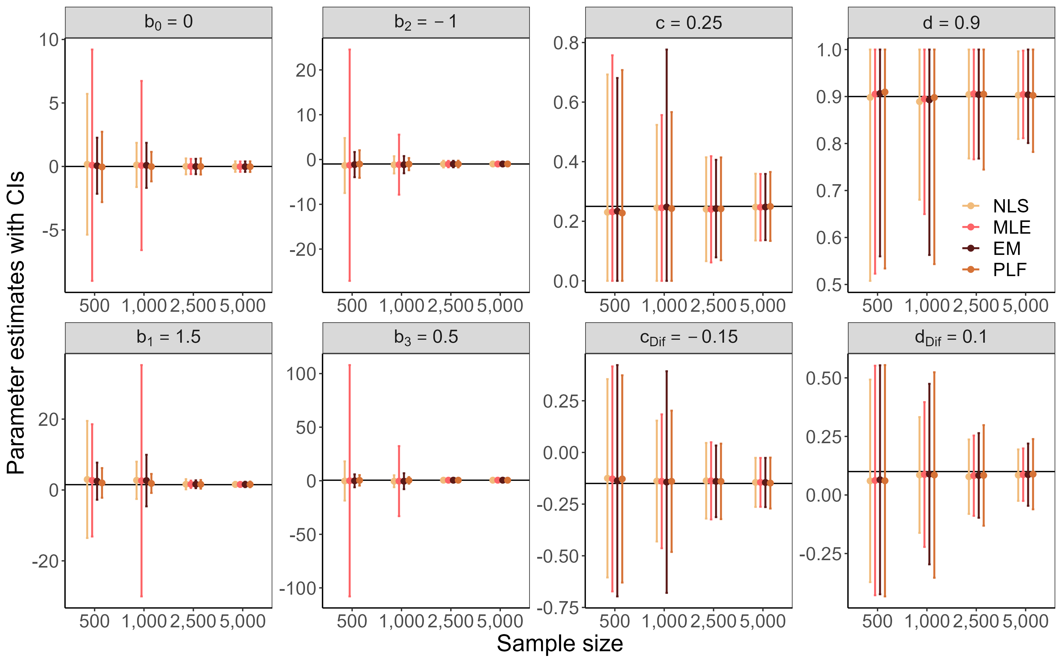
Figure 3: Mean estimated parameters in the group-specific 4PL model (3) with confidence intervals with respect to sample size; horizontal lines represent true values of parameters

4 Real data example

4.1 Data description

This study demonstrated the estimation on a real-data example of the PROMIS Anxiety scale dataset. The dataset consisted of responses to 29 Likert-type questions (1 = Never, 2 = Rarely, 3 = Sometimes, 4 = Often, and 5 = Always) from 766 respondents. Additionally, the dataset included information on the respondents’ age (0 = Younger than 65 and 1 = 65 and older), gender (0 = Male and 1 = Female), and education (0 = Some college or higher and 1 = High school or lower).

For this work, item responses were dichotomised as follows: 0 = Never (i.e., response $=1$ on original scale) or 1 = At least rarely (i.e., response $\geq 2$ on original scale). The overall level of anxiety was calculated as a standardised sum of non-dichotomized item responses. This work considered the simple 4PL model (1) and the group-specific 4PL model (3) using all four estimation methods: NLS, ML, the EM algorithm, and the algorithm based on PLF. In both models, the computed overall level of anxiety was used as the matching criterion $X_{p}$. In the group-specific 4PL model (3), respondents’ genders were included as the grouping variable $G_{p}$. Overall, there were 369 male participants and 397 female participants.

4.2 Analysis design

The same approach used in the simulation study for computing starting values was used for the analysis of the Anxiety dataset. In the case of convergence issues, the initial values were re-calculated based on successfully converged estimates using other methods.

In this study, item parameter estimates were computed and reported with their confidence intervals. Confidence intervals of the asymptote parameters were truncated at boundary values when necessary. Next, this work compared the estimation methods by calculating the differences in fitted item characteristic curves (i.e., estimated probabilities of endorsing the item) on the matching criterion for both models. Finally, likelihood ratio tests were performed to compare the two nested models (simple and group-specific) to identify the DIF for all items and all four estimation methods. Significance level of 0.05 was used for all the tests.

4.3 Results

Simple 4PL model.

The smallest differences between the four estimation methods and fitted item characteristic curves in the simple 4PL model (1) were observed for item R8 (”I had a racing or pounding heart”; Figure 4(a)). The greatest differences were observed for item R29 (”I had difficulty calming down”; Figure 4(b)). The smallest overall differences were found between the EM algorithm and the algorithm based on PLF, whereas the greatest overall differences were noted between the NLS and the algorithm based on PLF. Beyond this, similar patterns appeared in the estimated item parameters (Figure 5, Table LABEL:tab:anxiety:pars_simple). Although the lower asymptotes were mostly estimated at 0, the upper asymptotes were often estimated below 1, suggesting a reluctance of the respondents to admit certain difficulties, such as those due to social norms.

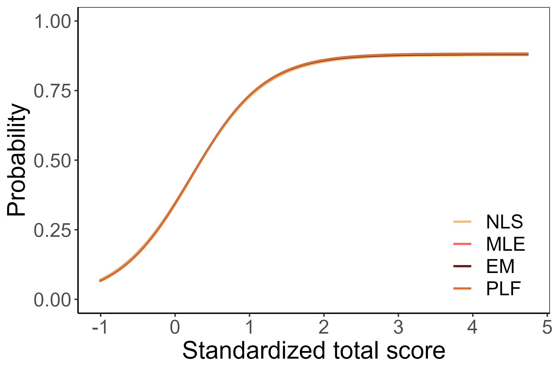
(a) Anxiety item R8

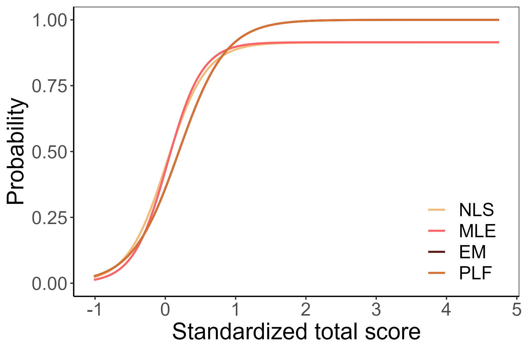
(b) Anxiety item R29

Figure 4: Estimated item characteristic curves for the simple 4PL model (1)

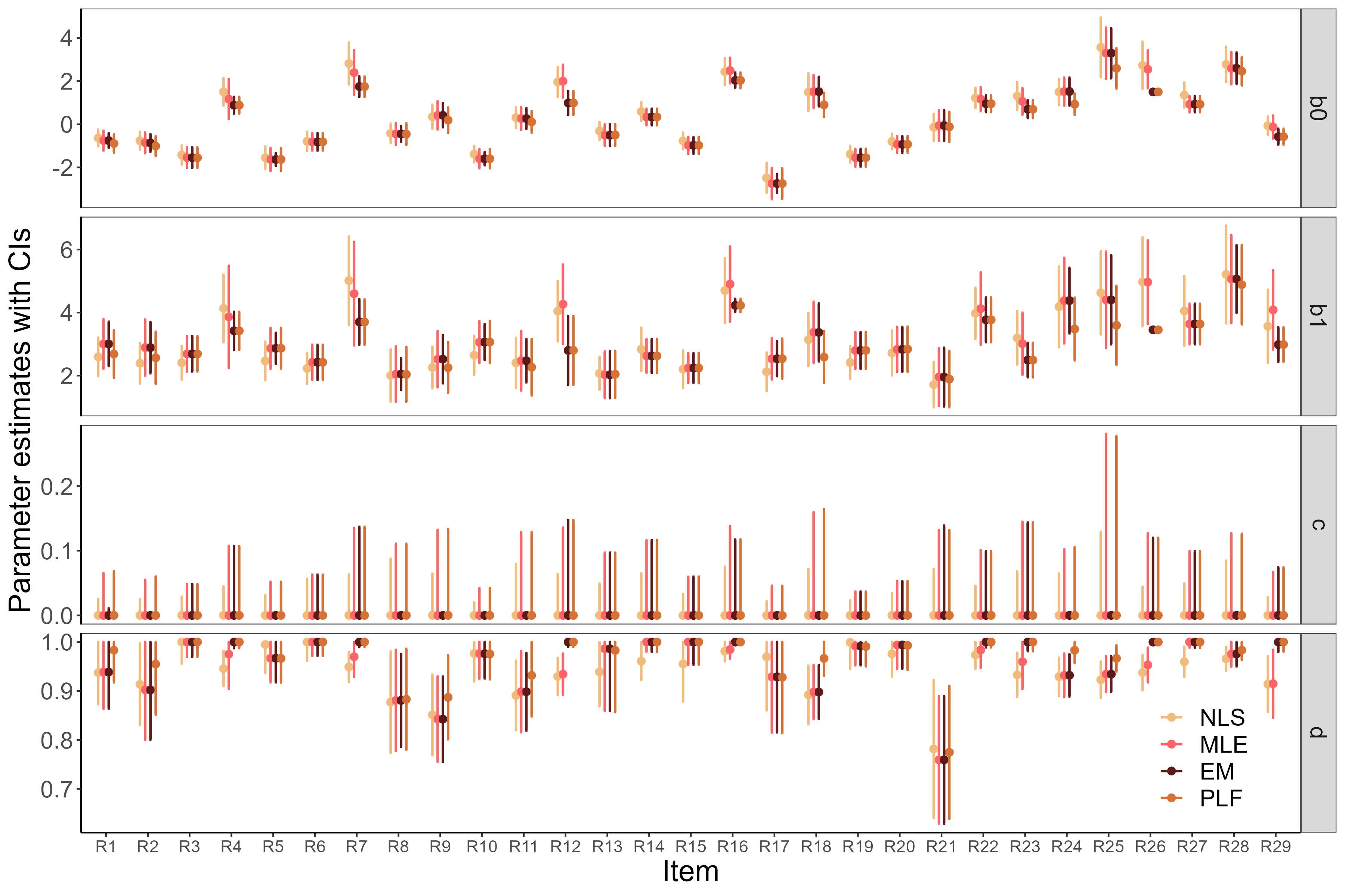
Figure 5: Item parameter estimates of the Anxiety items for the simple 4PL model (1).

Group-specific 4PL model.

The smallest differences between the four estimation algorithms and the fitted item characteristic curves in the group-specific 4PL model (3) were once more observed in item R8 (”I had a racing or pounding heart”; Figure 6(a)). The greatest differences were noticed in item R24 (”Many situations made me worry”; Figure 6(b)). The smallest overall differences were found between the EM algorithm and the algorithm based on PLF. The greatest overall differences were observed between the NLS and the algorithm based on PLF, analogous to the simple 4PL model. Additionally, similar patterns were seen in the estimated item parameters (Figure 7, Table LABEL:tab:anxiety:pars_dif).

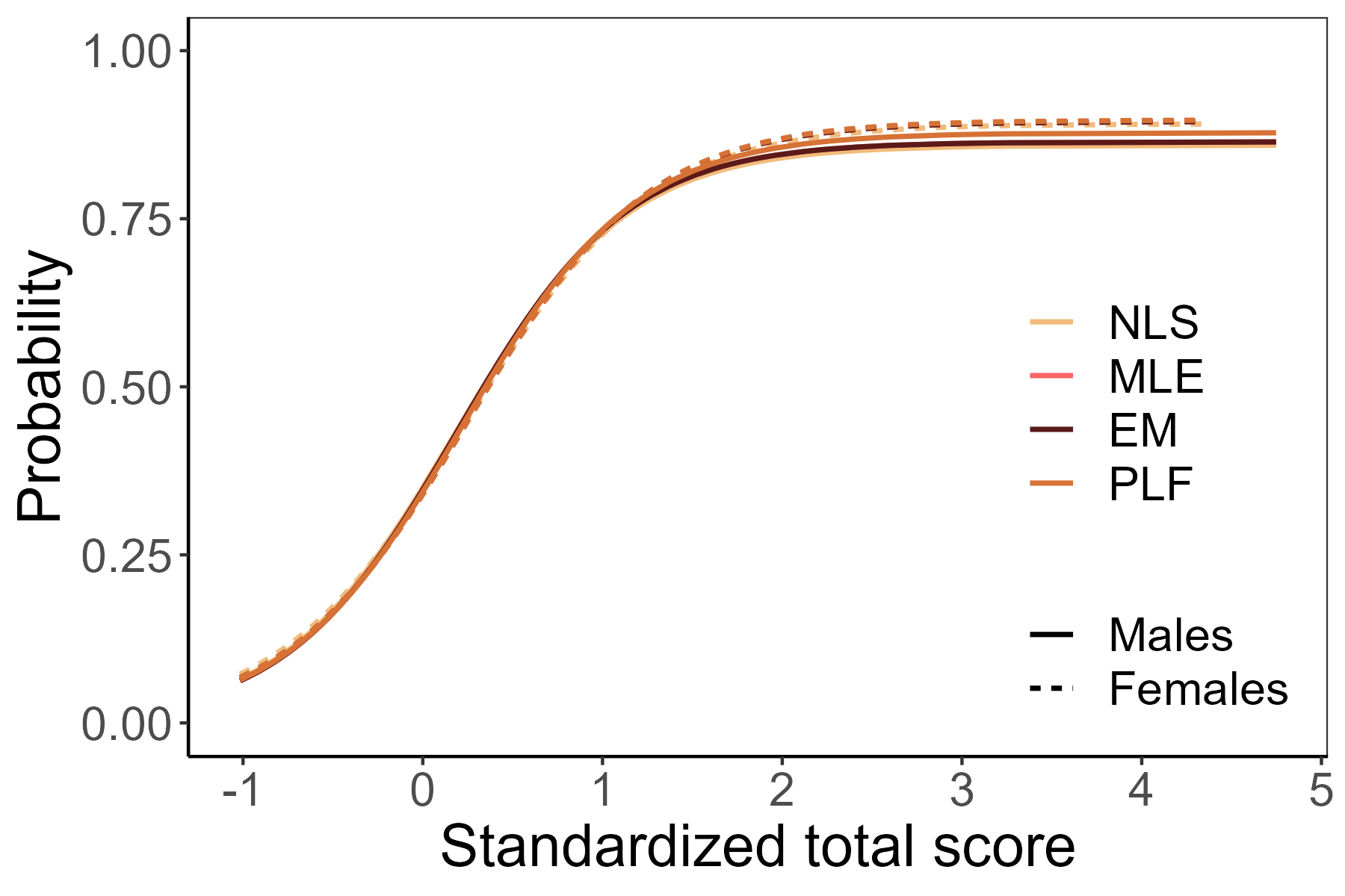
(a) Anxiety item R8

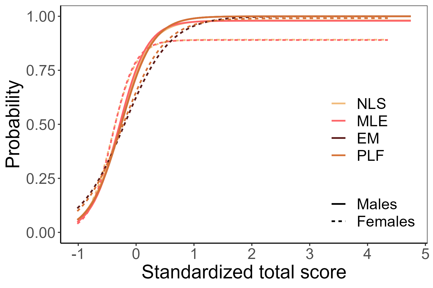
(b) Anxiety item R24

Figure 6: Estimated item characteristic curves for the group-specific 4PL model (3)

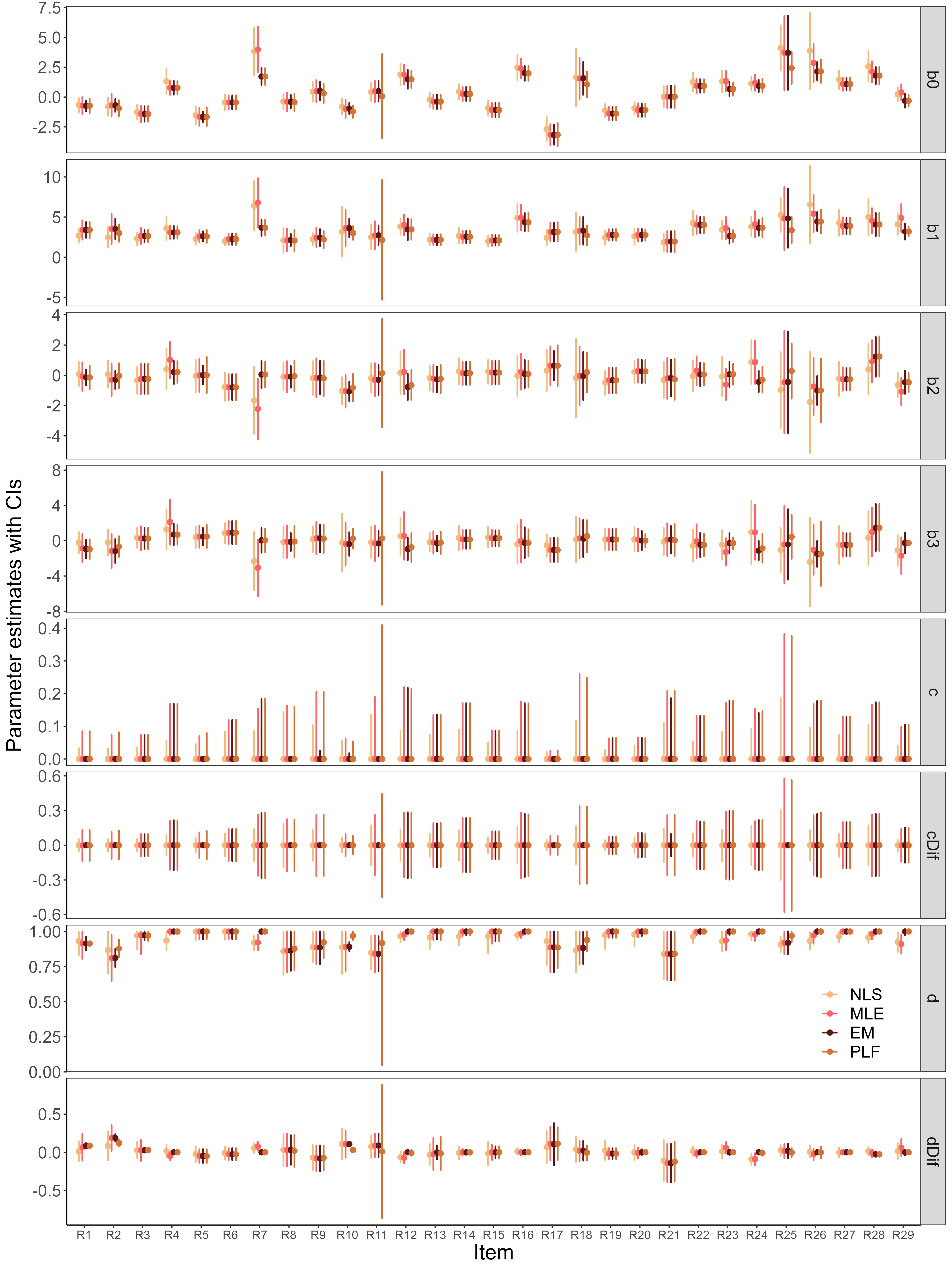
Figure 7: Item parameter estimates of the Anxiety items for the group-specific 4PL model (3)

DIF detection.

Using the likelihood ratio test, the simple 4PL model (1) was rejected for item R6 (”I was concerned about my mental health”), item R10 (”I had sudden feelings of panic”), and item R12 (”I had trouble paying attention”) when considering at least one estimation method (i.e., these items functioned differently). While item R6 was identified as a DIF item by all four of the estimation methods (all $p$-values $<0.004$), items R10 and R12 were only identified as functioning differently with the NLS ($p$-value = 0.042) and with the algorithm based on PLF ($p$-value = 0.047), respectively.

In item R6, there were no significant differences between the estimated asymptotes, and DIF was caused by various intercepts and slopes of the two genders (Figure 7). Male participants seemed to have a higher probability of being concerned about their mental health at least rarely (original response $\geq 2$) than female participants of the same overall anxiety level. This difference was especially apparent for those with lower levels of anxiety, whereas the differences between these two genders narrowed as the overall anxiety level increased (Figure 8).

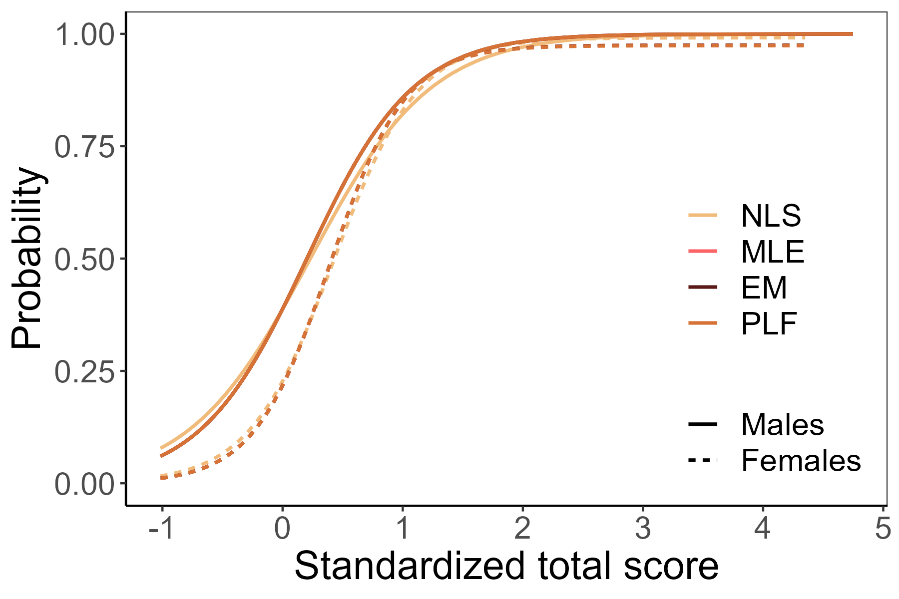
Figure 8: Estimated item characteristic curves for item R6 of the Anxiety dataset for the group-specific 4PL model (3)

5 Discussion

This work explored novel approaches for estimating item parameters in the generalised logistic regression model. We described in detail two existing procedures (NLS and ML) and their applications for fitting the covariate-specific 4PL model (2). Additionally, the study proposed two iterative procedures (a procedure using the EM algorithm and a method based on PLF). With a simulation study, we demonstrated satisfactory precision of the newly proposed PLF-based procedure even for small sample sizes and when additional covariates were considered. However, these pleasant properties were not observed for the NLS and ML methods, which produced either biased estimates or wide confidence intervals. On the other hand, the EM algorithm performed satisfactorily, but it sometimes failed to converge in a predefined number of iterations, so its fitting was inefficient. As the sample size increased, differences between the estimation methods vanished, and all estimates were near the true values of the item parameters.

Using a real data example for the anxiety measure, we illustrated practical challenges in estimation procedures, including specification of initial values. The smallest differences between the estimation procedures were observed for the EM algorithm and the procedure based on PLF. Additionally the largest dissimilarities were found for the NLS and the PLF-based method, supporting the findings of the simulation study, especially when considering a smaller sample size in the Anxiety dataset.

In recent decades, the topic of the parametric link function has been extensively discussed in the literature by many authors, including basu2005estimating, flach2014generalized, and scallan1984fitting. For example, pregibon1980goodness proposed the ML estimation of the link parameters using a weighted least squares algorithm. In the same vein, mccullagh1989generalized adapted this approach and presented an algorithm in which several models with the fixed link functions were fitted. Furthermore, kaiser1997maximum proposed a modified scoring algorithm to perform simultaneous ML estimation of all parameters. scallan1984fitting proposed an iterative two-stage algorithm, building on the work of richards1961method. In this study’s approach, we examined generalised logistic regression, accounting for the possibility of guessing and inattention or lapse rate, whereas these features may depend upon the respondents’ characteristics.

The crucial part of the estimation process is specifying starting values for item parameters because these values may significantly impact the speed of the estimation process and its precision. For instance, initial values which are far from the true item parameters may lead to situations in which the estimation algorithm returns only a local extreme or even it does not converge. In this work we used an approach based on upper-lower index which resulted in a low rate of convergence issues with the satisfactory estimation precision. However, other possible naive estimates of discrimination (and other parameters), such as a correlation between an item score and the total test score without given item, could be considered.

There were several limitations to this study, and several possible further directions for study exist. First, the simulation study was limited to two models – the simple 4PL model (1) and the group-specific 4PL model (3), both of which included only one or two covariates. The simulation study suggested requiring a larger sample size with the increasing number of covariates. Second, the work considered only one set of item parameters, noting that various values of asymptotes were especially prone to producing computational challenges. Third, this article described the NLS method as a simple approach, not accounting for the heteroscedasticity of binary data. For such data, the Pearson’s residuals might be more appropriate to use. This weighted form <e.g.,¿ritz2015dose takes the original squares of residuals and divides them by the variance $\pi_{pi}(1-\pi_{pi})$. Next, the RSS of item $i$ (4) would take the following form:

$$\text{RSS}_{i}(\boldsymbol{\gamma}_{i})=\sum_{p=1}^{n}\frac{\left(Y_{pi}-\pi_{pi}\right)^{2}}{\pi_{pi}\left(1-\pi_{pi}\right)}.$$

However, the number of observations on tails of the matching criterion is typically small and provides only small variability at most. These heavy weights would require a nearly exact fit for cases with few observations. Nevertheless, the computation of the NLS estimates demonstrated in this work was straightforward and efficient, providing sufficient precision. Thus, this method could be useful in certain cases, such as producing an initial idea about parameter values and using these estimates as starting values for other approaches.

Additionally, this study’s real data example explored item functioning in the multi-item measurement related to anxiety. However, the task of the parameter estimation in the presented models would also be relevant for several other situations. The later could include data from educational measurement, where the lower asymptote may represent item guessing, and the upper asymptote may represent the lapse rate (item slipping or inattention). Moreover, the generalised logistic regression model is not limited to multi-item measurements since the class determined by Equation (2) represents a wide family of the covariate-specific 4PL models. This model might be used and further extended in various study fields, including but not limited to quantitative pharmacology Dinse (2011); applied microbiology Brands . (2020); modelling patterns of urban electricity usage To . (2012); and plant growth modelling Zub . (2012). Therefore, estimating parameters and understanding limitations of used methods are crucial for a wide range of researchers and practitioners.

To conclude, this study illustrated differences and challenges in fitting generalised logistic regression models using various estimation techniques. This work demonstrated the superiority of the novel implementation of the EM algorithm and the newly proposed method based on PLF over the existing NLS and ML methods. Thus, improving the estimation algorithms is critical since it could increase precision while maintaining a user-friendly implementation.

Supplementary Material

Additional tables and figures, and accompanying R scripts are available at https://osf.io/bk8a7/.

Appendix A Asymptotics

A.1 Nonlinear least squares

Asymptotic properties of the NLS estimator, such as consistency and asymptotic distribution, can be derived under the classical set of regularity conditions <e.g.,¿[Theorems 5.41 and 5.42]van2000asymptotic. Next, one must reformulate these conditions for the covariate-specific 4PL model (2) considering $\boldsymbol{\gamma}_{iX}=(\boldsymbol{b}_{i},\boldsymbol{c}_{i},\boldsymbol{d}_{i})$ is a vector of true parameters:

1. A vector of true parameters $\boldsymbol{\gamma}_{iX}$ satisfies

   $$\operatorname{\textsf{E}}\left(\boldsymbol{\psi}_{i}(Y_{pi},\boldsymbol{X}_{p};\boldsymbol{\gamma}_{iX})\right)=\operatorname{\textsf{E}}\left(-2(Y_{pi}-\pi_{pi})\frac{\partial\pi_{pi}}{\partial\boldsymbol{\gamma}_{iX}}\right)=\boldsymbol{0}.$$

2. The true parameter $\boldsymbol{\gamma}_{iX}$ is an interior point of the parameter space.

3. The function $\boldsymbol{\psi}_{i}(y,\boldsymbol{x};\boldsymbol{\gamma}_{i})$ is twice continuously differentiable with respect to $\boldsymbol{\gamma}_{i}$ for every $(y,\boldsymbol{x})$.

4. For each $\boldsymbol{\gamma}_{i}^{\ast}$ in a neighbourhood of $\boldsymbol{\gamma}_{iX}$, there exists an integrable function $\ddot{\boldsymbol{\psi}}(y,\boldsymbol{x})$ such that

   $$\left|\frac{\partial^{2}\psi_{ik}(y,\boldsymbol{x};\boldsymbol{\gamma}_{i})}{\partial\gamma_{ij}\partial\gamma_{il}}\right|\leq\ddot{\boldsymbol{\psi}}(y,\boldsymbol{x}),\ \forall k,j,l.$$

5. The matrix

   $$\mathbb{\Gamma}_{i}(\boldsymbol{\gamma}_{i})= \ \operatorname{\textsf{E}}\left(\frac{\partial\boldsymbol{\psi}_{i}(Y_{pi},\boldsymbol{X}_{p};\boldsymbol{\gamma}_{i})}{\partial\boldsymbol{\gamma}_{i}^{\top}}\right)$$

   $$= \ 2\operatorname{\textsf{E}}\left(\frac{\partial\pi_{pi}}{\partial\boldsymbol{\gamma}_{i}}\left(\frac{\partial\pi_{pi}}{\partial\boldsymbol{\gamma}_{i}}\right)^{\top}-(Y_{pi}-\pi_{pi})\frac{\partial^{2}\pi_{pi}}{\partial\boldsymbol{\gamma}_{i}\partial\boldsymbol{\gamma}_{i}^{\top}}\right)$$

   $$= \ 2\operatorname{\textsf{E}}\left(\frac{\partial\pi_{pi}}{\partial\boldsymbol{\gamma}_{i}}\left(\frac{\partial\pi_{pi}}{\partial\boldsymbol{\gamma}_{i}}\right)^{\top}\right)$$

   is finite and regular in a neighbourhood of $\boldsymbol{\gamma}_{iX}$.

6. The variance matrix

   $$\mathbb{\Sigma}_{i}(\boldsymbol{\gamma}_{i})= \ \operatorname{\textsf{E}}\left(\boldsymbol{\psi}_{i}(Y_{pi},\boldsymbol{X}_{p};\boldsymbol{\gamma}_{i})\boldsymbol{\psi}_{i}^{\top}(Y_{pi},\boldsymbol{X}_{p};\boldsymbol{\gamma}_{i})\right)$$

   $$= \ 4\operatorname{\textsf{E}}\left(\left(Y_{pi}-\pi_{pi}\right)^{2}\frac{\partial\pi_{pi}}{\partial\boldsymbol{\gamma}_{i}}\left(\frac{\partial\pi_{pi}}{\partial\boldsymbol{\gamma}_{i}}\right)^{\top}\right)$$

   $$= \ 4\operatorname{\textsf{E}}\left(\pi_{pi}\left(1-\pi_{pi}\right)\frac{\partial\pi_{pi}}{\partial\boldsymbol{\gamma}_{i}}\left(\frac{\partial\pi_{pi}}{\partial\boldsymbol{\gamma}_{i}}\right)^{\top}\right)$$

   is finite for $\boldsymbol{\gamma}_{i}=\boldsymbol{\gamma}_{iX}$.

Specifically, Theorem 5.42 (van der Vaart, 1998, p. 68) implies that under the conditions [R0]–[R5], the probability that the estimating equations, $\frac{\partial\text{RSS}_{i}}{\partial\gamma_{ik}}=0$, have at least one root tends to 1, as $n\rightarrow\infty$, and there exists a sequence $\hat{\boldsymbol{\gamma}}_{i}$ (depending on $n$) such that $\hat{\boldsymbol{\gamma}}_{i}\stackrel{{\scriptstyle[}}{{n}}\rightarrow\infty]{P}{\longrightarrow}\boldsymbol{\gamma}_{iX}$. Moreover, the sequence $\hat{\boldsymbol{\gamma}}_{i}$ can be chosen to be a local maximum for each $n$. Theorem 5.41 (van der Vaart, 1998, p. 68) demonstrates that every consistent estimator $\hat{\boldsymbol{\gamma}}_{i}$ has asymptotically normal distribution, that is:

$$\sqrt{n}\left(\hat{\boldsymbol{\gamma}}_{i}-\boldsymbol{\gamma}_{iX}\right)\stackrel{{\scriptstyle[}}{{n}}\rightarrow\infty]{\mathcal{D}}{\longrightarrow}\mathcal{N}\left(\boldsymbol{0},\mathbb{\Gamma}_{i}^{-1}(\boldsymbol{\gamma}_{iX})\mathbb{\Sigma}_{i}(\boldsymbol{\gamma}_{iX})\mathbb{\Gamma}_{i}^{-1}(\boldsymbol{\gamma}_{iX})\right),$$

Clearly, the conditions [R0] and [R2] hold. To satisfy the condition [R1], one must bound asymptote parameters $\boldsymbol{c}_{i}$ and $\boldsymbol{d}_{i}$ to open intervals. If the asymptote parameters are on the boundary of the parameter space (e.g., $c_{i}=0$, $d_{i}=1$, and $c_{i\text{DIF}}=d_{i\text{DIF}}=0$ in the group-specific 4PL model (3)), the logistic regression model may be used instead. Additionally, the model (3) with some of the parameters fixed (e.g., $d_{i}=1$ and $d_{i\text{DIF}}=0$), may be considered analogously. Notably, the asymptotic properties derived here will hold for these submodels. However, it is not possible to test whether the full model or its submodel better fits the data using, for instance, likelihood ratio test. Regarding the condition [R3], in this case, a polynomial of $x$ of the fourth degree can be taken as an integrable dominating function.

Furthermore, because $\boldsymbol{X}_{p}$ describes respondent characteristics such as the standardised total score or gender, one can assume that their range is bounded, so the partial derivatives $\frac{\partial\pi_{pi}}{\partial\boldsymbol{\gamma}_{i}}$ are also bounded. Thus, matrices $\mathbb{\Gamma}_{i}(\boldsymbol{\gamma}_{i})$ and $\mathbb{\Sigma}_{i}(\boldsymbol{\gamma}_{i})$ are both finite, and the condition [R5] holds. Finally, when the rows or columns of the matrix $\mathbb{\Gamma}_{i}(\boldsymbol{\gamma}_{i})$ are linearly independent, the matrix has a full rank and thus is regular, satisfying condition [R4]. For instance, the singularity of the matrix may occur when $G_{p}=0,\forall p$ (or $G_{p}=1,\forall p$), meaning that all respondents are from the reference (or focal) group.

Therefore, all the assumptions [R1]–[R5] hold under the mild additional conditions, so $\hat{\boldsymbol{\gamma}}_{i}$ has desired asymptotic properties such as consistency and asymptotic normality of the item parameter estimates.

Estimate of asymptotic variance.

The natural estimate of the asymptotic variance of $\hat{\boldsymbol{\gamma}}_{i}$ is a sandwich estimator given by

$$\frac{1}{n}\widehat{\mathbb{\Gamma}}_{in}^{-1}(\hat{\boldsymbol{\gamma}}_{i})\widehat{\mathbb{\Sigma}}_{in}(\hat{\boldsymbol{\gamma}}_{i})\widehat{\mathbb{\Gamma}}_{in}^{-1}(\hat{\boldsymbol{\gamma}}_{i}),$$ (A1)

where

$$\widehat{\mathbb{\Gamma}}_{in}(\hat{\boldsymbol{\gamma}}_{i})= \ \frac{1}{n}\sum_{p=1}^{n}\left(\frac{\partial\boldsymbol{\psi}_{i}(Y_{pi},\boldsymbol{X}_{p};\hat{\boldsymbol{\gamma}}_{i})}{\partial\boldsymbol{\gamma}_{i}^{\top}}\right),$$

$$\widehat{\mathbb{\Sigma}}_{in}(\boldsymbol{\gamma}_{i})= \ \frac{1}{n}\sum_{p=1}^{n}\left(\boldsymbol{\psi}_{i}(Y_{pi},\boldsymbol{X}_{p};\hat{\boldsymbol{\gamma}}_{i})\boldsymbol{\psi}_{i}^{\top}(Y_{pi},\boldsymbol{X}_{p};\hat{\boldsymbol{\gamma}}_{i})\right),$$

with components of the matrix $\widehat{\mathbb{\Gamma}}_{in}(\boldsymbol{\gamma}_{i})=\nabla^{2}\text{RSS}_{i}(\boldsymbol{\gamma}_{i})$ being

$$\frac{\partial^{2}\text{RSS}_{i}(\boldsymbol{\gamma}_{i})}{\partial\gamma_{ik}\partial\gamma_{ij}}= \ -2\sum_{p=1}^{n}\left\{\left(Y_{pi}-\pi_{pi}\right)\frac{\partial^{2}\pi_{pi}}{\partial\gamma_{ik}\partial\gamma_{ij}}-\frac{\partial\pi_{pi}}{\partial\gamma_{ik}}\frac{\partial\pi_{pi}}{\partial\gamma_{ij}}\right\},$$

$$\frac{\partial^{2}\text{RSS}_{i}(\boldsymbol{\gamma}_{i})}{\partial\gamma_{ik}^{2}}= \ -2\sum_{p=1}^{n}\left\{\left(Y_{pi}-\pi_{pi}\right)\frac{\partial^{2}\pi_{pi}}{\partial\gamma_{ik}^{2}}-\left(\frac{\partial\pi_{pi}}{\partial\gamma_{ik}}\right)^{2}\right\}.$$

A.2 Maximum likelihood

Asymptotic properties of the ML estimator can be shown under the set of the following regularity conditions (van der Vaart, 1998, Theorems 5.41 and 5.42):

• The support set $S=\left\{y\in\mathbb{R}:f(y|\boldsymbol{x},\boldsymbol{\gamma}_{i})>0\right\}$ does not depend on the parameter $\boldsymbol{\gamma}_{i}$.

• The true parameter $\boldsymbol{\gamma}_{iX}$ is an interior point of the parameter space.

• The density $f(y|\boldsymbol{x},\boldsymbol{\gamma}_{i})=y\log\left(\pi(\boldsymbol{x};\boldsymbol{\gamma}_{i})\right)+(1-y)\log\left(1-\pi(\boldsymbol{x};\boldsymbol{\gamma}_{i})\right)$ is twice continuously differentiable with respect to $\boldsymbol{\gamma}_{i}$ for each $(y,\boldsymbol{x})$.

• The Fisher information matrix $\mathbb{I}_{i}(\boldsymbol{\gamma}_{i})$ is finite, regular, and positive definite in a neighbourhood of $\gamma_{iX}$.

• The order of differentiation and integration with respect to $\boldsymbol{\gamma}_{i}$ can be interchanged for terms $f(y|\boldsymbol{x},\boldsymbol{\gamma}_{i})$ and $\frac{\partial f(y|\boldsymbol{x},\boldsymbol{\gamma}_{i})}{\partial\boldsymbol{\gamma}_{i}}$.

Overall, the conditions [R0^∗] and [R2^∗] hold. In this case, the regularity condition for the ML estimator [R1^∗] is the same as condition [R1] for the NLS, so one must bound parameters of asymptotes to open intervals, as discussed in Section A.1.

For the condition [R3^∗], the Fisher information matrix takes the following form:

$$\mathbb{I}_{i}(\boldsymbol{\gamma}_{i})=\operatorname{\textsf{E}}\mathbb{I}_{i}(\boldsymbol{\gamma}_{i}|\boldsymbol{X}_{p})=\operatorname{\textsf{E}}\left(\frac{1}{\pi_{pi}\left(1-\pi_{pi}\right)}\frac{\partial\pi_{pi}}{\partial\gamma_{ik}}\frac{\partial\pi_{pi}}{\partial\gamma_{ij}}\right)_{k,j},$$

which is a quadratic form and thus positive definite. Again, $\boldsymbol{X}_{p}$ describes respondent characteristics, so one can assume that their range is bounded, meaning partial derivatives $\frac{\partial\pi_{pi}}{\partial\gamma_{ik}}$, making the Fisher information matrix finite. Similarly, as in Section A.1, when the rows or columns of the Fisher information matrix $\mathbb{I}_{i}(\boldsymbol{\gamma}_{i})$ are linearly independent, the matrix has a full rank and thus is regular, satisfying the condition [R3^∗]. The singularity of the matrix could occur in similar cases as for the matrix $\mathbb{\Gamma}_{i}(\boldsymbol{\gamma}_{i})$ described in Section A.1.

Finally, regarding the condition [R4^∗], the order of differentiation and integration can be interchanged by dominated convergence theorem, as far as both $\frac{\partial f(y|\boldsymbol{x},\boldsymbol{\gamma}_{i})}{\partial\boldsymbol{\gamma}_{i}}$ and $\frac{\partial^{2}f(y|\boldsymbol{x},\boldsymbol{\gamma}_{i})}{\partial\boldsymbol{\gamma}_{i}\partial\boldsymbol{\gamma}_{i}^{\top}}$ are dominated by an integrable function. In this case a polynomial of $x$ of the fourth degree can be taken as an integrable dominating function.

hogg2005introduction demonstrated that when the regularity conditions [R0^∗]–[R4^∗] hold, there exists $n_{0}\in\mathbf{N}$ and a sequence $\widehat{\boldsymbol{\gamma}}_{in}(n>n_{0})$ of solutions to the corresponding likelihood equations such that

$$\widehat{\boldsymbol{\gamma}}_{in}\stackrel{{\scriptstyle[}}{{n}}\rightarrow\infty]{P}{\longrightarrow}\boldsymbol{\gamma}_{iX},$$

where $\boldsymbol{\gamma}_{iX}$ is a vector of true parameters. Because the log-likelihood function is not strictly concave, the approach described does not guarantee finding a unique solution of the corresponding likelihood equations. Thus, there might be multiple solutions, each a local maximum. However, there is one solution among them, which provides a consistent sequence of estimators, whereas other solutions may not even be close to $\gamma_{iX}$ and may not converge to it. Therefore, in practice, the key part of estimating procedures is finding suitable starting values, preferably easily calculated but consistent estimate of parameters. Furthermore, for this consistent sequence of solutions it can be shown that

$$\sqrt{n}\left(\widehat{\boldsymbol{\gamma}}_{in}-\boldsymbol{\gamma}_{iX}\right)\stackrel{{\scriptstyle[}}{{n}}\rightarrow\infty]{\mathcal{D}}{\longrightarrow}\mathcal{N}(\boldsymbol{0},\mathbb{I}^{-1}_{i}(\boldsymbol{\gamma}_{iX})).$$

Estimate of asymptotic variance.

An estimate of the asymptotic variance of the item parameters $\hat{\boldsymbol{\gamma}}_{i}$ is an inverse of the observed information matrix, an inverse of the Hessian matrix as demonstrated here:

$$\mathbb{I}_{in}^{-1}(\hat{\boldsymbol{\gamma}}_{i}|\boldsymbol{X},\boldsymbol{G})=\left(-\frac{1}{n}\frac{\partial^{2}l_{i}(\hat{\boldsymbol{\gamma}}_{i})}{\partial\boldsymbol{\gamma}_{i}\partial\boldsymbol{\gamma}_{i}^{\top}}\right)^{-1}.$$ (A2)

Appendix B Tables

Table A1: Item parameter estimates with confidence intervals in parentheses by four estimation methods using the simple 4PL model (1) with respect to sample size

Parameter Method Sample size 500 1,000 2,500 5,000 $b_{0}=0$ NLS $0.57(-1.50,2.65)$ $-0.01(-0.76,0.75)$ $0.00(-0.41,0.42)$ $0.00(-0.28,0.29)$ MLE $-0.00(-1.56,1.56)$ $-0.02(-0.72,0.67)$ $-0.00(-0.41,0.40)$ $0.00(-0.28,0.28)$ EM $-0.01(-1.56,1.55)$ $-0.02(-0.71,0.66)$ $-0.00(-0.41,0.40)$ $-0.00(-0.28,0.28)$ PLF $0.00(-1.07,1.07)$ $-0.02(-0.71,0.66)$ $-0.00(-0.41,0.40)$ $-0.00(-0.28,0.28)$ $b_{1}=1.5$ NLS $4.32(-5.52,14.16)$ $1.81(-0.63,4.25)$ $1.58(0.85,2.30)$ $1.54(1.06,2.02)$ MLE $2.29(-6.09,10.66)$ $1.77\hphantom{-}(0.27,3.27)$ $1.57(0.89,2.25)$ $1.53(1.07,1.99)$ EM $2.23(-6.12,10.58)$ $1.76\hphantom{-}(0.39,3.14)$ $1.58(0.90,2.26)$ $1.54(1.08,2.01)$ PLF $1.87(-1.68,\hphantom{0}5.42)$ $1.72\hphantom{-}(0.43,3.01)$ $1.58(0.89,2.27)$ $1.55(1.09,2.02)$ $c=0.25$ NLS $0.25(0.00,0.55)$ $0.26(0.08,0.43)$ $0.25(0.14,0.36)$ $0.25(0.17,0.32)$ MLE $0.25(0.00,0.52)$ $0.26(0.08,0.43)$ $0.25(0.14,0.36)$ $0.25(0.17,0.32)$ EM $0.25(0.00,0.61)$ $0.26(0.08,0.43)$ $0.25(0.14,0.36)$ $0.25(0.18,0.32)$ PLF $0.25(0.00,0.52)$ $0.26(0.08,0.43)$ $0.25(0.14,0.36)$ $0.25(0.18,0.32)$ $d=0.9$ NLS $0.89(0.62,1.00)$ $0.89(0.75,1.00)$ $0.90(0.81,0.99)$ $0.90(0.84,0.96)$ MLE $0.89(0.68,1.00)$ $0.90(0.74,1.00)$ $0.90(0.81,0.99)$ $0.90(0.84,0.96)$ EM $0.89(0.63,1.00)$ $0.89(0.75,1.00)$ $0.90(0.81,0.99)$ $0.90(0.84,0.96)$ PLF $0.90(0.67,1.00)$ $0.90(0.74,1.00)$ $0.90(0.81,0.99)$ $0.90(0.84,0.96)$

x
Note. NLS = nonlinear least squares, MLE = maximum likelihood estimation, EM = expectation-maximisation algorithm, PLF = algorithm based on parametric link function.

Table A2: Item parameter estimates with confidence intervals in parentheses by four estimation methods using the group-specific 4PL model (3) with respect to sample size

Parameter Method Sample size 500 1,000 2,500 5,000 $b_{0}=0$ NLS $0.17(-5.37,5.72)$ $0.12(-1.62,1.86)$ $0.01(-0.62,0.63)$ $-0.01(-0.42,0.40)$ MLE $0.10(-9.01,9.21)$ $0.07(-6.59,6.73)$ $-0.00(-0.60,0.60)$ $-0.01(-0.42,0.39)$ EM $0.06(-2.15,2.26)$ $0.09(-1.69,1.86)$ $-0.00(-0.61,0.60)$ $-0.02(-0.43,0.40)$ PLF $-0.04(-2.81,2.73)$ $-0.01(-1.17,1.15)$ $-0.00(-0.63,0.63)$ $-0.02(-0.43,0.40)$ $b_{1}=1.5$ NLS $2.97(-13.55,19.49)$ $2.73\hphantom{0}(-2.53,\hphantom{0}7.99)$ $1.62(0.18,3.06)$ $1.57(0.85,2.29)$ MLE $2.71(-13.13,18.55)$ $2.61(-30.03,35.24)$ $1.60(0.57,2.64)$ $1.56(0.88,2.24)$ EM $2.49\hphantom{0}(-2.75,\hphantom{0}7.72)$ $2.66\hphantom{0}(-4.62,\hphantom{0}9.93)$ $1.61(0.51,2.72)$ $1.56(0.81,2.32)$ PLF $2.00\hphantom{0}(-2.18,\hphantom{0}6.18)$ $1.85\hphantom{0}(-0.83,\hphantom{0}4.53)$ $1.60(0.38,2.81)$ $1.57(0.77,2.38)$ $b_{2}=-1$ NLS $-1.35\hphantom{0}(-7.49,\hphantom{0}4.79)$ $-1.19(-3.11,0.73)$ $-1.02(-1.77,-0.27)$ $-1.00(-1.50,-0.50)$ MLE $-1.27(-27.09,24.55)$ $-1.15(-7.85,5.55)$ $-1.02(-1.73,-0.31)$ $-1.00(-1.49,-0.52)$ EM $-1.14\hphantom{0}(-3.94,\hphantom{0}1.67)$ $-1.16(-3.07,0.76)$ $-1.02(-1.74,-0.30)$ $-1.00(-1.49,-0.51)$ PLF $-1.01\hphantom{0}(-4.09,\hphantom{0}2.06)$ $-1.04(-2.40,0.32)$ $-1.01(-1.76,-0.27)$ $-0.99(-1.49,-0.50)$ $b_{3}=0.5$ NLS $-0.21\hphantom{0}(-18.50,\hphantom{0}18.07)$ $-0.46\hphantom{0}(-6.01,\hphantom{0}5.09)$ $0.50(-1.09,2.09)$ $0.51(-0.34,1.36)$ MLE $-0.01(-107.94,107.93)$ $-0.37(-33.05,32.31)$ $0.50(-0.72,1.71)$ $0.51(-0.29,1.32)$ EM $-0.07\hphantom{00}(-6.10,\hphantom{00}5.96)$ $-0.43\hphantom{0}(-7.84,\hphantom{0}6.98)$ $0.49(-0.83,1.81)$ $0.51(-0.40,1.42)$ PLF $0.36\hphantom{00}(-4.52,\hphantom{00}5.24)$ $0.34\hphantom{0}(-2.70,\hphantom{0}3.38)$ $0.50(-0.97,1.96)$ $0.49(-0.46,1.45)$ $c=0.25$ NLS $0.23(0.00,0.69)$ $0.24(0.00,0.52)$ $0.24(0.07,0.41)$ $0.25(0.14,0.36)$ MLE $0.23(0.00,0.76)$ $0.25(0.00,0.56)$ $0.24(0.06,0.42)$ $0.25(0.14,0.36)$ EM $0.23(0.00,0.68)$ $0.25(0.00,0.78)$ $0.24(0.08,0.41)$ $0.25(0.14,0.36)$ PLF $0.23(0.00,0.71)$ $0.24(0.00,0.57)$ $0.24(0.07,0.41)$ $0.25(0.13,0.37)$ $c_{\text{DIF}}=-0.15$ NLS $-0.13(-0.60,0.35)$ $-0.14(-0.43,0.15)$ $-0.14(-0.32,0.05)$ $-0.14(-0.26,-0.03)$ MLE $-0.13(-0.67,0.42)$ $-0.14(-0.46,0.18)$ $-0.14(-0.32,0.05)$ $-0.14(-0.26,-0.03)$ EM $-0.14(-0.70,0.42)$ $-0.14(-0.68,0.39)$ $-0.14(-0.31,0.03)$ $-0.15(-0.26,-0.03)$ PLF $-0.13(-0.63,0.37)$ $-0.14(-0.48,0.20)$ $-0.14(-0.32,0.04)$ $-0.15(-0.27,-0.02)$ $d=0.9$ NLS $0.90(0.51,1.00)$ $0.89(0.68,1.00)$ $0.90(0.77,1.00)$ $0.90(0.81,1.00)$ MLE $0.91(0.52,1.00)$ $0.90(0.65,1.00)$ $0.91(0.77,1.00)$ $0.90(0.81,1.00)$ EM $0.91(0.56,1.00)$ $0.89(0.56,1.00)$ $0.90(0.77,1.00)$ $0.90(0.80,1.00)$ PLF $0.91(0.53,1.00)$ $0.90(0.54,1.00)$ $0.91(0.74,1.00)$ $0.90(0.78,1.00)$ $d_{\text{DIF}}=0.1$ NLS $0.06(-0.37,0.49)$ $0.09(-0.16,0.33)$ $0.08(-0.08,0.24)$ $0.08(-0.02,0.19)$ MLE $0.06(-0.43,0.55)$ $0.09(-0.22,0.40)$ $0.08(-0.09,0.25)$ $0.09(-0.03,0.20)$ EM $0.06(-0.42,0.55)$ $0.09(-0.30,0.47)$ $0.08(-0.10,0.26)$ $0.09(-0.05,0.22)$ PLF $0.06(-0.43,0.55)$ $0.09(-0.35,0.52)$ $0.08(-0.13,0.30)$ $0.09(-0.06,0.24)$

x
Note. NLS = nonlinear least squares, MLE = maximum likelihood estimation, EM = expectation-maximisation algorithm, PLF = algorithm based on parametric link function.

Table A3: Item parameters estimates with standard errors in parentheses by four estimation methods using the simple 4PL model (1) for the Anxiety dataset

Item	Method	$b_{0}$	$b_{1}$	$c$	$d$
R1	NLS	$-0.64(0.20)$	$2.59(0.31)$	$0.00(0.01)$	$0.94(0.03)$
	MLE	$-0.76(0.23)$	$3.01(0.40)$	$0.00(0.03)$	$0.94(0.04)$
	EM	$-0.76(0.17)$	$3.01(0.36)$	$0.00(0.01)$	$0.94(0.04)$
	PLF	$-0.89(0.21)$	$2.69(0.38)$	$0.00(0.03)$	$0.98(0.03)$
R2	NLS	$-0.76(0.21)$	$2.39(0.33)$	$0.00(0.01)$	$0.91(0.04)$
	MLE	$-0.86(0.24)$	$2.89(0.45)$	$0.00(0.03)$	$0.90(0.05)$
	EM	$-0.86(0.20)$	$2.89(0.42)$	$0.00(\text{N\kern-1.00006pt/\kern-1.00006ptA})$	$0.90(0.05)$
	PLF	$-1.01(0.23)$	$2.57(0.42)$	$0.00(0.03)$	$0.96(0.05)$
R3	NLS	$-1.43(0.22)$	$2.41(0.27)$	$0.00(0.01)$	$1.00(0.02)$
	MLE	$-1.55(0.24)$	$2.69(0.28)$	$0.00(0.02)$	$1.00(0.02)$
	EM	$-1.55(0.24)$	$2.69(0.28)$	$0.00(0.02)$	$1.00(0.02)$
	PLF	$-1.55(0.24)$	$2.69(0.28)$	$0.00(0.02)$	$1.00(0.02)$
R4	NLS	$1.50(0.32)$	$4.13(0.55)$	$0.00(0.02)$	$0.95(0.02)$
	MLE	$1.17(0.47)$	$3.87(0.82)$	$0.00(0.05)$	$0.98(0.04)$
	EM	$0.88(0.20)$	$3.42(0.31)$	$0.00(0.05)$	$1.00(0.01)$
	PLF	$0.88(0.20)$	$3.42(0.31)$	$0.00(0.05)$	$1.00(0.01)$
R5	NLS	$-1.55(0.26)$	$2.47(0.31)$	$0.00(0.02)$	$0.99(0.03)$
	MLE	$-1.63(0.27)$	$2.87(0.33)$	$0.00(0.03)$	$0.97(0.02)$
	EM	$-1.63(0.15)$	$2.87(0.25)$	$0.00(\text{N\kern-1.00006pt/\kern-1.00006ptA})$	$0.97(0.02)$
	PLF	$-1.63(0.27)$	$2.87(0.33)$	$0.00(0.03)$	$0.97(0.03)$
R6	NLS	$-0.79(0.23)$	$2.23(0.25)$	$0.00(0.03)$	$1.00(0.02)$
	MLE	$-0.82(0.20)$	$2.42(0.28)$	$0.00(0.03)$	$1.00(0.01)$
	EM	$-0.82(0.20)$	$2.42(0.28)$	$0.00(0.03)$	$1.00(0.01)$
	PLF	$-0.82(0.20)$	$2.42(0.28)$	$0.00(0.03)$	$1.00(0.01)$
R7	NLS	$2.82(0.49)$	$5.01(0.71)$	$0.00(0.03)$	$0.95(0.02)$
	MLE	$2.40(0.52)$	$4.60(0.84)$	$0.00(0.07)$	$0.97(0.02)$
	EM	$1.75(0.24)$	$3.70(0.36)$	$0.00(0.07)$	$1.00(0.01)$
	PLF	$1.75(0.24)$	$3.70(0.36)$	$0.00(0.07)$	$1.00(0.01)$
R8	NLS	$-0.42(0.23)$	$2.00(0.42)$	$0.00(0.04)$	$0.88(0.05)$
	MLE	$-0.45(0.25)$	$2.05(0.45)$	$0.00(0.06)$	$0.88(0.05)$
	EM	$-0.45(0.18)$	$2.05(0.25)$	$0.00(\text{N\kern-1.00006pt/\kern-1.00006ptA})$	$0.88(0.05)$
	PLF	$-0.46(0.25)$	$2.04(0.44)$	$0.00(0.06)$	$0.88(0.05)$
R9	NLS	$0.34(0.29)$	$2.26(0.34)$	$0.00(0.03)$	$0.85(0.04)$
	MLE	$0.41(0.33)$	$2.52(0.45)$	$0.00(0.07)$	$0.84(0.04)$
	EM	$0.41(0.28)$	$2.52(0.39)$	$0.00(\text{N\kern-1.00006pt/\kern-1.00006ptA})$	$0.84(0.04)$
	PLF	$0.19(0.30)$	$2.25(0.41)$	$0.00(0.07)$	$0.89(0.04)$
R10	NLS	$-1.39(0.19)$	$2.65(0.31)$	$0.00(0.01)$	$0.98(0.03)$
	MLE	$-1.60(0.22)$	$3.06(0.34)$	$0.00(0.02)$	$0.98(0.03)$
	EM	$-1.60(0.15)$	$3.06(0.29)$	$0.00(\text{N\kern-1.00006pt/\kern-1.00006ptA})$	$0.98(0.03)$
	PLF	$-1.60(0.22)$	$3.07(0.34)$	$0.00(0.02)$	$0.98(0.03)$
R11	NLS	$0.31(0.24)$	$2.41(0.40)$	$0.00(0.04)$	$0.89(0.04)$
	MLE	$0.27(0.26)$	$2.47(0.48)$	$0.00(0.07)$	$0.90(0.04)$
	EM	$0.27(0.24)$	$2.47(0.35)$	$0.00(\text{N\kern-1.00006pt/\kern-1.00006ptA})$	$0.90(0.04)$
	PLF	$0.11(0.25)$	$2.27(0.45)$	$0.00(0.07)$	$0.93(0.04)$
R12	NLS	$1.96(0.35)$	$4.04(0.49)$	$0.00(0.03)$	$0.93(0.02)$
	MLE	$2.00(0.39)$	$4.26(0.64)$	$0.00(0.07)$	$0.93(0.02)$
	EM	$0.99(0.28)$	$2.80(0.56)$	$0.00(0.08)$	$1.00(0.00)$
	PLF	$0.99(0.28)$	$2.80(0.56)$	$0.00(0.08)$	$1.00(0.00)$
R13	NLS	$-0.31(0.21)$	$2.07(0.27)$	$0.00(0.03)$	$0.94(0.04)$
	MLE	$-0.51(0.25)$	$2.03(0.38)$	$0.00(0.05)$	$0.99(0.06)$
	EM	$-0.51(0.25)$	$2.03(0.38)$	$0.00(0.05)$	$0.99(0.06)$
	PLF	$-0.50(0.25)$	$2.04(0.38)$	$0.00(0.05)$	$0.98(0.06)$
R14	NLS	$0.59(0.22)$	$2.84(0.35)$	$0.00(0.03)$	$0.96(0.02)$
	MLE	$0.34(0.19)$	$2.62(0.27)$	$0.00(0.06)$	$1.00(0.01)$
	EM	$0.34(0.19)$	$2.62(0.27)$	$0.00(0.06)$	$1.00(0.01)$
	PLF	$0.34(0.19)$	$2.62(0.27)$	$0.00(0.06)$	$1.00(0.01)$
R15	NLS	$-0.77(0.19)$	$2.20(0.30)$	$0.00(0.02)$	$0.96(0.04)$
	MLE	$-0.98(0.20)$	$2.24(0.24)$	$0.00(0.03)$	$1.00(0.02)$
	EM	$-0.98(0.20)$	$2.24(0.24)$	$0.00(0.03)$	$1.00(0.02)$
	PLF	$-0.98(0.20)$	$2.24(0.24)$	$0.00(0.03)$	$1.00(0.02)$
R16	NLS	$2.44(0.32)$	$4.70(0.52)$	$0.00(0.04)$	$0.98(0.01)$
	MLE	$2.49(0.30)$	$4.90(0.61)$	$0.00(0.07)$	$0.98(0.01)$
	EM	$2.03(0.18)$	$4.23(0.10)$	$0.00(0.06)$	$1.00(\text{N\kern-1.00006pt/\kern-1.00006ptA})$
	PLF	$2.03(0.18)$	$4.23(0.10)$	$0.00(0.06)$	$1.00(\text{N\kern-1.00006pt/\kern-1.00006ptA})$
R17	NLS	$-2.49(0.35)$	$2.12(0.31)$	$0.00(0.01)$	$0.97(0.06)$
	MLE	$-2.75(0.37)$	$2.54(0.33)$	$0.00(0.02)$	$0.93(0.06)$
	EM	$-2.75(0.22)$	$2.54(0.28)$	$0.00(\text{N\kern-1.00006pt/\kern-1.00006ptA})$	$0.93(0.06)$
	PLF	$-2.75(0.35)$	$2.54(0.32)$	$0.00(0.02)$	$0.93(0.06)$
R18	NLS	$1.49(0.44)$	$3.14(0.43)$	$0.00(0.04)$	$0.89(0.03)$
	MLE	$1.51(0.39)$	$3.37(0.50)$	$0.00(0.08)$	$0.90(0.03)$
	EM	$1.51(0.35)$	$3.37(0.47)$	$0.00(\text{N\kern-1.00006pt/\kern-1.00006ptA})$	$0.90(0.03)$
	PLF	$0.90(0.28)$	$2.59(0.42)$	$0.00(0.08)$	$0.97(0.02)$
R19	NLS	$-1.38(0.19)$	$2.42(0.26)$	$0.00(0.01)$	$1.00(0.03)$
	MLE	$-1.55(0.21)$	$2.80(0.30)$	$0.00(0.02)$	$0.99(0.02)$
	EM	$-1.55(0.21)$	$2.80(0.30)$	$0.00(0.02)$	$0.99(0.02)$
	PLF	$-1.55(0.21)$	$2.80(0.30)$	$0.00(0.02)$	$0.99(0.02)$
R20	NLS	$-0.80(0.18)$	$2.72(0.36)$	$0.00(0.02)$	$0.98(0.02)$
	MLE	$-0.93(0.19)$	$2.83(0.36)$	$0.00(0.03)$	$0.99(0.02)$
	EM	$-0.93(0.19)$	$2.83(0.36)$	$0.00(0.03)$	$0.99(0.02)$
	PLF	$-0.93(0.19)$	$2.84(0.36)$	$0.00(0.03)$	$0.99(0.03)$
R21	NLS	$-0.14(0.32)$	$1.72(0.37)$	$0.00(0.04)$	$0.78(0.07)$
	MLE	$-0.06(0.36)$	$1.95(0.46)$	$0.00(0.07)$	$0.76(0.07)$
	EM	$-0.06(0.36)$	$1.95(0.47)$	$0.00(0.07)$	$0.76(0.07)$
	PLF	$-0.12(0.35)$	$1.89(0.45)$	$0.00(0.07)$	$0.77(0.07)$
R22	NLS	$1.22(0.24)$	$3.98(0.41)$	$0.00(0.02)$	$0.97(0.01)$
	MLE	$1.16(0.28)$	$4.12(0.59)$	$0.00(0.05)$	$0.98(0.02)$
	EM	$0.95(0.20)$	$3.77(0.36)$	$0.00(0.05)$	$1.00(0.01)$
	PLF	$0.95(0.20)$	$3.77(0.36)$	$0.00(0.05)$	$1.00(0.01)$
R23	NLS	$1.31(0.33)$	$3.20(0.43)$	$0.00(0.03)$	$0.93(0.02)$
	MLE	$1.06(0.31)$	$3.01(0.50)$	$0.00(0.07)$	$0.96(0.03)$
	EM	$0.70(0.21)$	$2.49(0.28)$	$0.00(0.07)$	$1.00(0.01)$
	PLF	$0.70(0.21)$	$2.49(0.28)$	$0.00(0.07)$	$1.00(0.01)$
R24	NLS	$1.50(0.30)$	$4.19(0.65)$	$0.00(0.03)$	$0.93(0.02)$
	MLE	$1.52(0.33)$	$4.38(0.69)$	$0.00(0.05)$	$0.93(0.02)$
	EM	$1.52(0.33)$	$4.38(0.53)$	$0.00(0.00)$	$0.93(0.02)$
	PLF	$0.93(0.25)$	$3.48(0.51)$	$0.00(0.05)$	$0.98(0.01)$
R25	NLS	$3.57(0.70)$	$4.63(0.67)$	$0.00(0.07)$	$0.92(0.02)$
	MLE	$3.30(0.60)$	$4.40(0.78)$	$0.00(0.14)$	$0.93(0.02)$
	EM	$3.30(0.59)$	$4.41(0.72)$	$0.00(\text{N\kern-1.00006pt/\kern-1.00006ptA})$	$0.93(0.02)$
	PLF	$2.59(0.47)$	$3.59(0.64)$	$0.00(0.14)$	$0.97(0.01)$
R26	NLS	$2.74(0.56)$	$4.97(0.72)$	$0.00(0.02)$	$0.94(0.02)$
	MLE	$2.55(0.45)$	$4.96(0.68)$	$0.00(0.06)$	$0.95(0.02)$
	EM	$1.50(\text{N\kern-1.00006pt/\kern-1.00006ptA})$	$3.45(\text{N\kern-1.00006pt/\kern-1.00006ptA})$	$0.00(0.06)$	$1.00(\text{N\kern-1.00006pt/\kern-1.00006ptA})$
	PLF	$1.50(\text{N\kern-1.00006pt/\kern-1.00006ptA})$	$3.45(\text{N\kern-1.00006pt/\kern-1.00006ptA})$	$0.00(0.06)$	$1.00(\text{N\kern-1.00006pt/\kern-1.00006ptA})$
R27	NLS	$1.35(0.29)$	$4.05(0.57)$	$0.00(0.03)$	$0.96(0.02)$
	MLE	$0.93(0.19)$	$3.64(0.33)$	$0.00(0.05)$	$1.00(0.01)$
	EM	$0.93(0.19)$	$3.64(0.33)$	$0.00(0.05)$	$1.00(0.01)$
	PLF	$0.93(0.19)$	$3.64(0.33)$	$0.00(0.05)$	$1.00(0.01)$
R28	NLS	$2.78(0.42)$	$5.21(0.79)$	$0.00(0.04)$	$0.97(0.01)$
	MLE	$2.60(0.38)$	$5.06(0.71)$	$0.00(0.06)$	$0.98(0.01)$
	EM	$2.60(0.37)$	$5.06(0.55)$	$0.00(0.00)$	$0.98(0.01)$
	PLF	$2.46(0.33)$	$4.88(0.64)$	$0.00(0.06)$	$0.98(0.01)$
R29	NLS	$-0.07(0.22)$	$3.57(0.59)$	$0.00(0.01)$	$0.91(0.03)$
	MLE	$-0.13(0.27)$	$4.08(0.64)$	$0.00(0.03)$	$0.91(0.04)$
	EM	$-0.57(0.19)$	$2.98(0.28)$	$0.00(0.04)$	$1.00(0.01)$
	PLF	$-0.57(0.19)$	$2.98(0.28)$	$0.00(0.04)$	$1.00(0.01)$

Table A4: Item parameters estimates with standard errors in parentheses by four estimation methods using the group-specific 4PL model (3) for the Anxiety dataset

Item	Method	$b_{0}$	$b_{1}$	$b_{2}$	$b_{3}$	$c$	$c_{\text{DIF}}$	$d$	$d_{\text{DIF}}$
R1	NLS	$-0.68(0.32)$	$2.69(0.44)$	$0.08(0.40)$	$-0.21(0.61)$	$0.00(0.02)$	$0.00(0.03)$	$0.93(0.05)$	$0.01(0.07)$
	MLE	$-0.73(0.36)$	$3.39(0.61)$	$-0.09(0.48)$	$-0.83(0.83)$	$0.00(0.04)$	$0.00(0.07)$	$0.92(0.06)$	$0.07(0.09)$
	EM	$-0.73(0.22)$	$3.39(0.49)$	$-0.14(0.26)$	$-0.95(0.53)$	$0.00(\text{N\kern-1.00006pt/\kern-1.00006ptA})$	$-0.00(\text{N\kern-1.00006pt/\kern-1.00006ptA})$	$0.92(0.02)$	$0.08(0.02)$
	PLF	$-0.73(0.31)$	$3.39(0.51)$	$-0.14(0.40)$	$-0.95(0.56)$	$0.00(0.04)$	$0.00(0.07)$	$0.91(\text{N\kern-1.00006pt/\kern-1.00006ptA})$	$0.09(\text{N\kern-1.00006pt/\kern-1.00006ptA})$
R2	NLS	$-0.80(0.36)$	$2.47(0.64)$	$0.07(0.44)$	$-0.18(0.73)$	$0.00(0.02)$	$0.00(0.03)$	$0.87(0.08)$	$0.08(0.09)$
	MLE	$-0.70(0.48)$	$3.52(0.96)$	$-0.29(0.54)$	$-1.17(1.00)$	$0.00(0.04)$	$0.00(0.06)$	$0.81(0.08)$	$0.19(0.09)$
	EM	$-0.70(0.27)$	$3.52(0.65)$	$-0.29(0.31)$	$-1.17(0.68)$	$0.00(\text{N\kern-1.00006pt/\kern-1.00006ptA})$	$-0.00(\text{N\kern-1.00006pt/\kern-1.00006ptA})$	$0.81(0.03)$	$0.19(0.02)$
	PLF	$-0.95(0.34)$	$3.01(0.54)$	$-0.04(0.42)$	$-0.66(0.59)$	$0.00(0.04)$	$0.00(0.06)$	$0.88(0.03)$	$0.12(0.02)$
R3	NLS	$-1.26(0.30)$	$2.30(0.39)$	$-0.32(0.45)$	$0.33(0.57)$	$0.00(0.02)$	$0.00(0.03)$	$0.97(0.05)$	$0.03(0.05)$
	MLE	$-1.42(0.34)$	$2.64(0.52)$	$-0.23(0.51)$	$0.26(0.70)$	$0.00(0.04)$	$0.00(0.05)$	$0.97(0.07)$	$0.03(0.07)$
	EM	$-1.42(0.33)$	$2.64(0.39)$	$-0.23(0.50)$	$0.26(0.60)$	$0.00(0.04)$	$-0.00(0.05)$	$0.97(0.02)$	$0.03(0.01)$
	PLF	$-1.42(0.33)$	$2.65(0.39)$	$-0.23(0.50)$	$0.25(0.60)$	$0.00(0.04)$	$0.00(0.05)$	$0.97(0.02)$	$0.03(0.01)$
R4	NLS	$1.32(0.55)$	$3.58(0.76)$	$0.40(0.68)$	$1.29(1.15)$	$0.00(0.03)$	$0.00(0.05)$	$0.94(0.04)$	$0.02(0.04)$
	MLE	$0.77(0.29)$	$3.08(0.40)$	$1.02(0.61)$	$2.12(1.30)$	$0.00(0.09)$	$0.00(0.11)$	$1.00(0.01)$	$-0.05(0.03)$
	EM	$0.77(0.29)$	$3.08(0.39)$	$0.21(0.39)$	$0.70(0.61)$	$0.00(0.09)$	$-0.00(0.11)$	$1.00(0.01)$	$0.00(0.01)$
	PLF	$0.77(0.28)$	$3.08(0.39)$	$0.21(0.37)$	$0.70(0.58)$	$0.00(0.09)$	$0.00(0.11)$	$1.00(0.01)$	$-0.00(\text{N\kern-1.00006pt/\kern-1.00006ptA})$
R5	NLS	$-1.54(0.39)$	$2.29(0.37)$	$-0.04(0.54)$	$0.39(0.63)$	$0.00(0.02)$	$0.00(0.03)$	$1.00(0.03)$	$-0.02(0.05)$
	MLE	$-1.67(0.37)$	$2.61(0.39)$	$0.01(0.56)$	$0.47(0.64)$	$0.00(0.04)$	$0.00(0.06)$	$1.00(0.03)$	$-0.05(0.04)$
	EM	$-1.67(0.21)$	$2.61(0.30)$	$0.01(0.30)$	$0.47(0.48)$	$0.00(0.00)$	$-0.00(0.01)$	$1.00(0.03)$	$-0.05(0.04)$
	PLF	$-1.67(0.40)$	$2.61(0.41)$	$0.01(0.61)$	$0.47(0.67)$	$0.00(0.04)$	$0.00(0.06)$	$1.00(0.03)$	$-0.05(0.04)$
R6	NLS	$-0.46(0.32)$	$1.98(0.25)$	$-0.76(0.47)$	$0.87(0.57)$	$0.00(0.04)$	$0.00(0.05)$	$1.00(0.03)$	$-0.01(0.04)$
	MLE	$-0.46(0.30)$	$2.26(0.35)$	$-0.79(0.44)$	$0.91(0.67)$	$0.00(0.06)$	$0.00(0.07)$	$1.00(0.03)$	$-0.03(0.04)$
	EM	$-0.46(0.30)$	$2.26(0.36)$	$-0.79(0.44)$	$0.91(0.67)$	$0.00(0.06)$	$-0.00(0.07)$	$1.00(0.03)$	$-0.03(0.04)$
	PLF	$-0.46(0.30)$	$2.26(0.36)$	$-0.79(0.44)$	$0.91(0.67)$	$0.00(0.06)$	$0.00(0.07)$	$1.00(0.03)$	$-0.03(0.04)$
R7	NLS	$3.81(1.02)$	$6.40(1.57)$	$-1.66(1.12)$	$-2.30(1.70)$	$0.00(0.04)$	$0.00(0.07)$	$0.92(0.03)$	$0.06(0.03)$
	MLE	$3.99(0.97)$	$6.79(1.55)$	$-2.22(1.02)$	$-3.07(1.63)$	$0.00(0.08)$	$0.00(0.13)$	$0.92(0.03)$	$0.08(0.03)$
	EM	$1.72(0.36)$	$3.68(0.52)$	$0.05(0.46)$	$0.04(0.71)$	$0.00(0.09)$	$-0.00(0.14)$	$1.00(0.01)$	$0.00(0.01)$
	PLF	$1.72(0.35)$	$3.68(0.49)$	$0.05(0.44)$	$0.04(0.67)$	$0.00(0.09)$	$0.00(0.14)$	$1.00(0.01)$	$0.00(\text{N\kern-1.00006pt/\kern-1.00006ptA})$
R8	NLS	$-0.37(0.33)$	$2.09(0.80)$	$-0.08(0.46)$	$-0.15(0.94)$	$0.00(0.07)$	$0.00(0.10)$	$0.86(0.09)$	$0.03(0.11)$
	MLE	$-0.40(0.38)$	$2.12(0.70)$	$-0.09(0.51)$	$-0.13(0.91)$	$0.00(0.08)$	$0.00(0.11)$	$0.86(0.08)$	$0.03(0.11)$
	EM	$-0.40(0.29)$	$2.11(0.39)$	$-0.09(0.37)$	$-0.13(0.52)$	$0.00(0.00)$	$-0.00(\text{N\kern-1.00006pt/\kern-1.00006ptA})$	$0.86(0.07)$	$0.03(0.10)$
	PLF	$-0.44(0.38)$	$2.07(0.67)$	$-0.05(0.51)$	$-0.09(0.89)$	$0.00(0.08)$	$0.00(0.11)$	$0.88(0.08)$	$0.02(0.11)$
R9	NLS	$0.45(0.43)$	$2.23(0.38)$	$-0.19(0.57)$	$0.17(0.73)$	$0.00(0.05)$	$0.00(0.07)$	$0.89(0.06)$	$-0.07(0.08)$
	MLE	$0.50(0.46)$	$2.45(0.60)$	$-0.16(0.65)$	$0.29(0.93)$	$0.00(0.10)$	$0.00(0.13)$	$0.89(0.06)$	$-0.08(0.09)$
	EM	$0.50(0.39)$	$2.45(0.52)$	$-0.16(0.56)$	$0.28(0.79)$	$0.00(0.01)$	$-0.00(0.01)$	$0.89(0.06)$	$-0.08(0.09)$
	PLF	$0.31(0.42)$	$2.23(0.54)$	$-0.19(0.59)$	$0.22(0.83)$	$0.00(0.11)$	$0.00(0.13)$	$0.92(0.06)$	$-0.07(0.08)$
R10	NLS	$-0.80(0.33)$	$3.17(1.57)$	$-1.02(0.45)$	$-0.21(1.65)$	$0.00(0.03)$	$0.00(0.03)$	$0.89(0.10)$	$0.11(0.10)$
	MLE	$-0.98(0.39)$	$3.62(1.15)$	$-1.06(0.55)$	$-0.37(1.24)$	$0.00(0.03)$	$0.00(0.05)$	$0.89(0.09)$	$0.11(0.09)$
	EM	$-0.98(0.24)$	$3.63(0.60)$	$-1.06(0.33)$	$-0.37(0.68)$	$0.00(0.01)$	$-0.00(\text{N\kern-1.00006pt/\kern-1.00006ptA})$	$0.89(0.02)$	$0.11(0.01)$
	PLF	$-1.22(0.26)$	$3.01(0.42)$	$-0.81(0.45)$	$0.24(0.57)$	$0.00(0.03)$	$0.00(0.04)$	$0.97(0.01)$	$0.03(0.01)$
R11	NLS	$0.42(0.38)$	$2.50(0.78)$	$-0.18(0.49)$	$-0.17(0.89)$	$0.00(0.07)$	$0.00(0.09)$	$0.85(0.06)$	$0.07(0.07)$
	MLE	$0.49(0.45)$	$2.72(0.89)$	$-0.30(0.56)$	$-0.31(1.03)$	$0.00(0.10)$	$0.00(0.13)$	$0.84(0.07)$	$0.09(0.08)$
	EM	$0.49(0.44)$	$2.72(0.63)$	$-0.30(0.50)$	$-0.30(0.73)$	$0.00(0.00)$	$-0.00(0.00)$	$0.84(0.06)$	$0.09(0.08)$
	PLF	$0.06(1.80)$	$2.15(3.79)$	$0.14(1.83)$	$0.27(3.83)$	$0.00(0.21)$	$0.00(0.23)$	$0.92(0.44)$	$0.01(0.45)$
R12	NLS	$1.87(0.45)$	$3.82(0.52)$	$0.17(0.72)$	$0.53(1.08)$	$0.00(0.04)$	$0.00(0.07)$	$0.97(0.02)$	$-0.06(0.04)$
	MLE	$1.88(0.42)$	$4.03(0.65)$	$0.22(0.75)$	$0.55(1.37)$	$0.00(0.11)$	$0.00(0.14)$	$0.98(0.02)$	$-0.07(0.04)$
	EM	$1.48(0.40)$	$3.45(0.69)$	$-0.77(0.43)$	$-0.96(0.63)$	$0.00(0.11)$	$-0.00(0.14)$	$1.00(0.00)$	$0.00(0.01)$
	PLF	$1.48(0.38)$	$3.46(0.64)$	$-0.65(0.51)$	$-0.74(0.85)$	$0.00(0.11)$	$0.00(0.14)$	$1.00(0.00)$	$-0.01(0.02)$
R13	NLS	$-0.21(0.31)$	$2.18(0.37)$	$-0.18(0.42)$	$-0.17(0.54)$	$0.00(0.04)$	$0.00(0.05)$	$0.96(0.04)$	$-0.03(0.07)$
	MLE	$-0.39(0.30)$	$2.16(0.35)$	$-0.22(0.47)$	$-0.19(0.65)$	$0.00(0.07)$	$0.00(0.10)$	$1.00(0.03)$	$-0.02(0.11)$
	EM	$-0.39(0.30)$	$2.16(0.34)$	$-0.27(0.42)$	$-0.28(0.44)$	$0.00(0.07)$	$-0.00(0.10)$	$1.00(0.03)$	$0.00(0.04)$
	PLF	$-0.39(0.30)$	$2.16(0.35)$	$-0.24(0.47)$	$-0.23(0.65)$	$0.00(0.07)$	$0.00(0.10)$	$1.00(0.03)$	$-0.01(0.11)$
R14	NLS	$0.45(0.31)$	$2.66(0.48)$	$0.26(0.44)$	$0.32(0.69)$	$0.00(0.05)$	$0.00(0.07)$	$0.96(0.03)$	$-0.01(0.04)$
	MLE	$0.26(0.29)$	$2.54(0.40)$	$0.14(0.39)$	$0.15(0.54)$	$0.00(0.09)$	$0.00(0.12)$	$1.00(0.02)$	$0.00(0.02)$
	EM	$0.26(0.29)$	$2.54(0.39)$	$0.14(0.39)$	$0.15(0.53)$	$0.00(0.09)$	$-0.00(0.12)$	$1.00(0.01)$	$0.00(0.02)$
	PLF	$0.26(0.29)$	$2.54(0.39)$	$0.14(0.39)$	$0.15(0.53)$	$0.00(0.09)$	$0.00(0.12)$	$1.00(0.01)$	$0.00(0.02)$
R15	NLS	$-0.92(0.32)$	$1.98(0.33)$	$0.24(0.40)$	$0.40(0.59)$	$0.00(0.03)$	$0.00(0.03)$	$0.97(0.06)$	$-0.01(0.08)$
	MLE	$-1.08(0.31)$	$2.09(0.34)$	$0.18(0.40)$	$0.28(0.47)$	$0.00(0.04)$	$0.00(0.06)$	$1.00(0.04)$	$0.00(0.05)$
	EM	$-1.08(0.31)$	$2.09(0.32)$	$0.18(0.40)$	$0.28(0.45)$	$0.00(0.04)$	$-0.00(0.06)$	$1.00(0.03)$	$0.00(0.04)$
	PLF	$-1.08(0.31)$	$2.09(0.32)$	$0.18(0.40)$	$0.28(0.45)$	$0.00(0.04)$	$0.00(0.06)$	$1.00(0.03)$	$0.00(0.04)$
R16	NLS	$2.47(0.55)$	$4.90(0.89)$	$-0.03(0.68)$	$-0.38(1.09)$	$0.00(0.04)$	$0.00(0.08)$	$0.97(0.02)$	$0.01(0.02)$
	MLE	$2.37(0.41)$	$4.92(0.81)$	$0.24(0.60)$	$-0.03(1.20)$	$0.00(0.09)$	$0.00(0.14)$	$0.99(0.01)$	$-0.00(0.02)$
	EM	$1.99(0.31)$	$4.34(0.57)$	$0.09(0.48)$	$-0.24(0.89)$	$0.00(0.09)$	$-0.00(0.14)$	$1.00(\text{N\kern-1.00006pt/\kern-1.00006ptA})$	$0.00(0.00)$
	PLF	$1.99(0.31)$	$4.34(0.57)$	$0.09(0.44)$	$-0.24(0.78)$	$0.00(0.09)$	$0.00(0.14)$	$1.00(\text{N\kern-1.00006pt/\kern-1.00006ptA})$	$-0.00(\text{N\kern-1.00006pt/\kern-1.00006ptA})$
R17	NLS	$-2.67(0.51)$	$2.43(0.48)$	$0.31(0.70)$	$-0.53(0.63)$	$0.00(0.01)$	$0.00(0.02)$	$0.93(0.09)$	$0.07(0.11)$
	MLE	$-3.17(0.45)$	$3.14(0.59)$	$0.64(0.65)$	$-1.05(0.69)$	$0.00(0.01)$	$0.00(0.04)$	$0.89(0.09)$	$0.11(0.11)$
	EM	$-3.17(0.41)$	$3.14(0.58)$	$0.64(0.49)$	$-1.04(0.68)$	$0.00(\text{N\kern-1.00006pt/\kern-1.00006ptA})$	$-0.00(0.00)$	$0.89(0.09)$	$0.11(0.14)$
	PLF	$-3.17(0.50)$	$3.15(0.61)$	$0.64(0.68)$	$-1.05(0.70)$	$0.00(0.01)$	$0.00(0.04)$	$0.89(0.08)$	$0.11(0.11)$
R18	NLS	$1.64(1.24)$	$3.17(1.20)$	$-0.18(1.32)$	$0.14(1.31)$	$0.00(0.06)$	$0.00(0.08)$	$0.87(0.08)$	$0.04(0.09)$
	MLE	$1.55(0.88)$	$3.28(0.87)$	$-0.02(0.98)$	$0.27(1.16)$	$0.00(0.13)$	$0.00(0.17)$	$0.88(0.06)$	$0.02(0.07)$
	EM	$1.57(0.70)$	$3.31(0.88)$	$-0.05(0.82)$	$0.23(1.07)$	$0.00(0.00)$	$-0.00(0.00)$	$0.88(0.06)$	$0.02(0.07)$
	PLF	$1.07(0.54)$	$2.71(0.60)$	$0.21(0.66)$	$0.53(0.91)$	$0.00(0.13)$	$0.00(0.17)$	$0.94(0.04)$	$-0.01(0.05)$
R19	NLS	$-1.12(0.29)$	$2.43(0.44)$	$-0.48(0.41)$	$0.17(0.61)$	$0.00(0.01)$	$0.00(0.02)$	$0.98(0.05)$	$0.02(0.06)$
	MLE	$-1.39(0.29)$	$2.77(0.36)$	$-0.33(0.42)$	$0.14(0.59)$	$0.00(0.03)$	$0.00(0.04)$	$1.00(0.02)$	$-0.02(0.03)$
	EM	$-1.39(0.29)$	$2.77(0.36)$	$-0.33(0.43)$	$0.14(0.59)$	$0.00(0.03)$	$-0.00(0.04)$	$1.00(0.02)$	$-0.02(0.04)$
	PLF	$-1.39(0.29)$	$2.77(0.36)$	$-0.33(0.43)$	$0.14(0.59)$	$0.00(0.03)$	$0.00(0.04)$	$1.00(0.02)$	$-0.02(0.04)$
R20	NLS	$-0.94(0.27)$	$2.58(0.50)$	$0.22(0.37)$	$0.16(0.69)$	$0.00(0.02)$	$0.00(0.03)$	$0.98(0.04)$	$0.00(0.05)$
	MLE	$-1.09(0.28)$	$2.76(0.41)$	$0.29(0.39)$	$0.11(0.65)$	$0.00(0.03)$	$0.00(0.05)$	$1.00(0.02)$	$-0.01(0.04)$
	EM	$-1.09(0.28)$	$2.76(0.40)$	$0.26(0.39)$	$0.02(0.57)$	$0.00(0.03)$	$-0.00(0.05)$	$1.00(0.02)$	$0.00(0.02)$
	PLF	$-1.09(0.28)$	$2.76(0.35)$	$0.26(0.39)$	$0.02(0.36)$	$0.00(0.03)$	$0.00(0.05)$	$1.00(\text{N\kern-1.00006pt/\kern-1.00006ptA})$	$-0.00(\text{N\kern-1.00006pt/\kern-1.00006ptA})$
R21	NLS	$0.03(0.45)$	$1.84(0.54)$	$-0.31(0.61)$	$-0.10(0.79)$	$0.00(0.06)$	$0.00(0.07)$	$0.84(0.09)$	$-0.11(0.14)$
	MLE	$0.03(0.48)$	$1.95(0.67)$	$-0.19(0.70)$	$0.13(0.94)$	$0.00(0.11)$	$0.00(0.13)$	$0.84(0.10)$	$-0.14(0.13)$
	EM	$0.03(0.47)$	$1.95(0.64)$	$-0.19(0.61)$	$0.13(0.77)$	$0.00(0.09)$	$-0.00(0.05)$	$0.84(0.10)$	$-0.14(0.13)$
	PLF	$0.02(0.48)$	$1.95(0.67)$	$-0.26(0.69)$	$0.05(0.93)$	$0.00(0.11)$	$0.00(0.13)$	$0.84(0.10)$	$-0.12(0.13)$
R22	NLS	$1.26(0.39)$	$4.28(0.78)$	$-0.05(0.51)$	$-0.57(0.90)$	$0.00(0.03)$	$0.00(0.05)$	$0.96(0.02)$	$0.01(0.03)$
	MLE	$0.94(0.31)$	$4.04(0.57)$	$0.30(0.48)$	$-0.06(0.98)$	$0.00(0.07)$	$0.00(0.11)$	$1.00(0.01)$	$-0.02(0.03)$
	EM	$0.93(0.28)$	$4.02(0.52)$	$0.06(0.39)$	$-0.47(0.70)$	$0.00(0.07)$	$-0.00(0.10)$	$1.00(0.01)$	$0.00(0.01)$
	PLF	$0.93(0.28)$	$4.02(0.51)$	$0.06(0.37)$	$-0.47(0.66)$	$0.00(0.07)$	$0.00(0.10)$	$1.00(0.01)$	$-0.00(\text{N\kern-1.00006pt/\kern-1.00006ptA})$
R23	NLS	$1.33(0.45)$	$3.41(0.57)$	$-0.06(0.66)$	$-0.47(0.84)$	$0.00(0.04)$	$0.00(0.07)$	$0.93(0.03)$	$0.01(0.05)$
	MLE	$1.34(0.43)$	$3.63(0.71)$	$-0.61(0.52)$	$-1.27(0.78)$	$0.00(0.09)$	$0.00(0.15)$	$0.94(0.04)$	$0.06(0.04)$
	EM	$0.67(0.31)$	$2.64(0.48)$	$0.06(0.43)$	$-0.28(0.57)$	$0.00(0.09)$	$-0.00(0.15)$	$1.00(0.01)$	$0.00(0.02)$
	PLF	$0.67(0.28)$	$2.64(0.36)$	$0.06(0.35)$	$-0.28(0.33)$	$0.00(0.09)$	$0.00(0.15)$	$1.00(0.00)$	$0.00(\text{N\kern-1.00006pt/\kern-1.00006ptA})$
R24	NLS	$1.12(0.30)$	$3.83(0.63)$	$0.86(0.74)$	$0.96(1.83)$	$0.00(0.05)$	$0.00(0.09)$	$0.98(0.02)$	$-0.09(0.04)$
	MLE	$1.21(0.34)$	$4.11(0.82)$	$0.87(0.73)$	$0.94(1.57)$	$0.00(0.08)$	$0.00(0.11)$	$0.98(0.02)$	$-0.09(0.04)$
	EM	$0.94(0.26)$	$3.67(0.50)$	$-0.43(0.36)$	$-1.12(0.57)$	$0.00(0.07)$	$-0.00(0.11)$	$1.00(\text{N\kern-1.00006pt/\kern-1.00006ptA})$	$0.00(\text{N\kern-1.00006pt/\kern-1.00006ptA})$
	PLF	$0.94(0.29)$	$3.67(0.62)$	$-0.30(0.43)$	$-0.86(0.82)$	$0.00(0.07)$	$0.00(0.11)$	$1.00(0.01)$	$-0.01(0.02)$
R25	NLS	$4.11(0.97)$	$5.23(1.09)$	$-0.96(1.28)$	$-1.06(1.27)$	$0.00(0.10)$	$0.00(0.15)$	$0.91(0.03)$	$0.03(0.04)$
	MLE	$3.71(1.59)$	$4.83(2.01)$	$-0.45(1.72)$	$-0.42(2.22)$	$0.00(0.20)$	$0.00(0.29)$	$0.92(0.04)$	$0.02(0.05)$
	EM	$3.71(1.58)$	$4.83(1.86)$	$-0.45(1.71)$	$-0.42(2.03)$	$0.00(0.00)$	$-0.00(0.00)$	$0.92(0.04)$	$0.02(0.05)$
	PLF	$2.43(0.68)$	$3.35(0.84)$	$0.28(0.93)$	$0.44(1.26)$	$0.00(0.19)$	$0.00(0.29)$	$0.97(0.02)$	$-0.00(0.03)$
R26	NLS	$3.88(1.63)$	$6.56(2.46)$	$-1.77(1.71)$	$-2.41(2.54)$	$0.00(0.05)$	$0.00(0.07)$	$0.93(0.03)$	$0.01(0.04)$
	MLE	$2.87(0.81)$	$5.42(1.18)$	$-0.74(0.96)$	$-1.03(1.44)$	$0.00(0.09)$	$0.00(0.13)$	$0.97(0.03)$	$-0.02(0.04)$
	EM	$2.15(0.39)$	$4.43(0.60)$	$-1.00(0.49)$	$-1.49(0.74)$	$0.00(0.09)$	$-0.00(0.14)$	$1.00(0.01)$	$0.00(0.01)$
	PLF	$2.15(0.48)$	$4.43(0.74)$	$-1.00(1.07)$	$-1.49(1.83)$	$0.00(0.09)$	$0.00(0.14)$	$1.00(0.01)$	$-0.00(0.04)$
R27	NLS	$1.45(0.39)$	$4.27(0.81)$	$-0.23(0.58)$	$-0.48(1.10)$	$0.00(0.04)$	$0.00(0.05)$	$0.96(0.02)$	$-0.00(0.03)$
	MLE	$1.08(0.28)$	$3.91(0.53)$	$-0.26(0.38)$	$-0.46(0.68)$	$0.00(0.07)$	$0.00(0.10)$	$1.00(0.01)$	$0.00(0.01)$
	EM	$1.08(0.27)$	$3.91(0.52)$	$-0.26(0.37)$	$-0.47(0.67)$	$0.00(0.07)$	$-0.00(0.10)$	$1.00(0.01)$	$0.00(0.01)$
	PLF	$1.08(0.27)$	$3.91(0.52)$	$-0.26(0.37)$	$-0.47(0.67)$	$0.00(0.07)$	$0.00(0.10)$	$1.00(0.01)$	$0.00(0.01)$
R28	NLS	$2.57(0.65)$	$5.02(1.15)$	$0.39(0.85)$	$0.33(1.58)$	$0.00(0.05)$	$0.00(0.09)$	$0.96(0.02)$	$0.02(0.03)$
	MLE	$2.12(0.44)$	$4.54(0.79)$	$0.92(0.71)$	$1.00(1.39)$	$0.00(0.08)$	$0.00(0.13)$	$0.98(0.02)$	$-0.01(0.02)$
	EM	$1.80(0.38)$	$4.07(0.74)$	$1.24(0.67)$	$1.47(1.37)$	$0.00(0.09)$	$-0.00(0.14)$	$1.00(0.00)$	$-0.03(0.02)$
	PLF	$1.80(0.38)$	$4.07(0.74)$	$1.24(0.68)$	$1.47(1.37)$	$0.00(0.09)$	$0.00(0.14)$	$1.00(0.00)$	$-0.03(0.02)$
R29	NLS	$0.22(0.30)$	$4.08(0.65)$	$-0.64(0.41)$	$-1.10(0.87)$	$0.00(0.02)$	$0.00(0.03)$	$0.92(0.04)$	$0.02(0.05)$
	MLE	$0.39(0.34)$	$4.90(0.89)$	$-1.07(0.46)$	$-1.69(1.05)$	$0.00(0.05)$	$0.00(0.07)$	$0.91(0.03)$	$0.06(0.06)$
	EM	$-0.32(0.28)$	$3.20(0.50)$	$-0.46(0.38)$	$-0.25(0.60)$	$0.00(0.05)$	$-0.00(0.08)$	$1.00(0.01)$	$0.00(0.02)$
	PLF	$-0.32(0.25)$	$3.20(0.31)$	$-0.46(0.33)$	$-0.25(0.11)$	$0.00(0.05)$	$0.00(0.08)$	$1.00(\text{N\kern-1.00006pt/\kern-1.00006ptA})$	$-0.00(\text{N\kern-1.00006pt/\kern-1.00006ptA})$

References

- Agresti (\APACyear2010) \APACinsertmetastaragresti2010analysis{APACrefauthors}Agresti, A. \APACrefYear2010. \APACrefbtitleAnalysis of ordinal categorical data Analysis of ordinal categorical data (\PrintOrdinalSecond \BEd). \APACaddressPublisherJohn Wiley & Sons. {APACrefDOI} \doi10.1002/9780470594001 \PrintBackRefs\CurrentBib
- Barton \BBA Lord (\APACyear1981) \APACinsertmetastarbarton1981upper{APACrefauthors}Barton, M\BPBIA.\BCBT \BBA Lord, F\BPBIM. \APACrefYearMonthDay1981. \BBOQ\APACrefatitleAn upper asymptote for the three-parameter logistic item-response model An upper asymptote for the three-parameter logistic item-response model.\BBCQ \APACjournalVolNumPagesETS Research Report Series198111–8. {APACrefDOI} \doi10.1007/s13398-014-0173-7.2 \PrintBackRefs\CurrentBib
- Basu \BBA Rathouz (\APACyear2005) \APACinsertmetastarbasu2005estimating{APACrefauthors}Basu, A.\BCBT \BBA Rathouz, P\BPBIJ. \APACrefYearMonthDay2005. \BBOQ\APACrefatitleEstimating marginal and incremental effects on health outcomes using flexible link and variance function models Estimating marginal and incremental effects on health outcomes using flexible link and variance function models.\BBCQ \APACjournalVolNumPagesBiostatistics6193–109. {APACrefDOI} \doi10.1093/biostatistics/kxh020 \PrintBackRefs\CurrentBib
- Birnbaum (\APACyear1968) \APACinsertmetastarbirnbaum1968statistical{APACrefauthors}Birnbaum, A. \APACrefYearMonthDay1968. \BBOQ\APACrefatitleSome latent trait models and their use in inferring an examinee’s ability Some latent trait models and their use in inferring an examinee’s ability.\BBCQ \BIn F\BPBIM. Lord \BBA M\BPBIR. Novick (\BEDS), \APACrefbtitleStatistical theories of mental test scores Statistical theories of mental test scores (\BPGS 397–479). \APACaddressPublisherAddison-Wesley, Reading, MA. \PrintBackRefs\CurrentBib
- Brands \BOthers. (\APACyear2020) \APACinsertmetastarbrands2020method{APACrefauthors}Brands, B., Schulze Struchtrup, S., Stamminger, R.\BCBL \BBA Bockmühl, D\BPBIP. \APACrefYearMonthDay2020. \BBOQ\APACrefatitleA method to evaluate factors influencing the microbial reduction in domestic dishwashers A method to evaluate factors influencing the microbial reduction in domestic dishwashers.\BBCQ \APACjournalVolNumPagesJournal of Applied Microbiology12851324–1338. {APACrefDOI} \doi10.1111/jam.14564 \PrintBackRefs\CurrentBib
- Byrd \BOthers. (\APACyear1995) \APACinsertmetastarbyrd1995limited{APACrefauthors}Byrd, R\BPBIH., Lu, P., Nocedal, J.\BCBL \BBA Zhu, C. \APACrefYearMonthDay1995. \BBOQ\APACrefatitleA limited memory algorithm for bound constrained optimization A limited memory algorithm for bound constrained optimization.\BBCQ \APACjournalVolNumPagesSIAM Journal on Scientific Computing1651190–1208. {APACrefDOI} \doi10.1137/0916069 \PrintBackRefs\CurrentBib
- Dempster \BOthers. (\APACyear1977) \APACinsertmetastardempster1977maximum{APACrefauthors}Dempster, A\BPBIP., Laird, N\BPBIM.\BCBL \BBA Rubin, D\BPBIB. \APACrefYearMonthDay1977. \BBOQ\APACrefatitleMaximum likelihood from incomplete data via the EM algorithm Maximum likelihood from incomplete data via the EM algorithm.\BBCQ \APACjournalVolNumPagesJournal of the Royal Statistical Society: Series B (Methodological)3911–22. {APACrefDOI} \doi10.1111/j.2517-6161.1977.tb01600.x \PrintBackRefs\CurrentBib
- Dennis \BOthers. (\APACyear1981) \APACinsertmetastardennis1981adaptive{APACrefauthors}Dennis, J\BPBIE\BPBIJ., Gay, D\BPBIM.\BCBL \BBA Welsch, R\BPBIE. \APACrefYearMonthDay1981. \BBOQ\APACrefatitleAn Adaptive Nonlinear Least-Squares Algorithm An adaptive nonlinear least-squares algorithm.\BBCQ \APACjournalVolNumPagesTransactions on Mathematical Software73348–368. {APACrefDOI} \doi10.1145/355958.355965 \PrintBackRefs\CurrentBib
- Dinse (\APACyear2011) \APACinsertmetastardinse2011algorithm{APACrefauthors}Dinse, G\BPBIE. \APACrefYearMonthDay2011. \BBOQ\APACrefatitleAn EM algorithm for fitting a four-parameter logistic model to binary dose-response data An EM algorithm for fitting a four-parameter logistic model to binary dose-response data.\BBCQ \APACjournalVolNumPagesJournal of Agricultural, Biological, and Environmental Statistics162221–232. {APACrefDOI} \doi10.1007/s13253-010-0045-3 \PrintBackRefs\CurrentBib
- Flach (\APACyear2014) \APACinsertmetastarflach2014generalized{APACrefauthors}Flach, N. \APACrefYear2014. \APACrefbtitleGeneralized linear models with parametric link families in R Generalized linear models with parametric link families in R \APACtypeAddressSchool\BUMTh. \APACaddressSchoolMünchenTechnische Universität München, Department of Mathematics. \PrintBackRefs\CurrentBib
- Gay (\APACyear\bibnodate) \APACinsertmetastarport{APACrefauthors}Gay, D. \APACrefYearMonthDay\bibnodate. \APACrefbtitlePort library documentation. Port library documentation. \APAChowpublishedhttp://www.netlib.org/port/. \APACrefnoteAccessed: 2022-12-13 \PrintBackRefs\CurrentBib
- Guidotti (\APACyear2022) \APACinsertmetastarguidotti2022calculus{APACrefauthors}Guidotti, E. \APACrefYearMonthDay2022. \BBOQ\APACrefatitlecalculus: High-Dimensional Numerical and Symbolic Calculus in R calculus: High-dimensional numerical and symbolic calculus in R.\BBCQ \APACjournalVolNumPagesJournal of Statistical Software10451–37. {APACrefDOI} \doi10.18637/jss.v104.i05 \PrintBackRefs\CurrentBib
- Hladká \BBA Martinková (\APACyear2020) \APACinsertmetastarhladka2020difnlr{APACrefauthors}Hladká, A.\BCBT \BBA Martinková, P. \APACrefYearMonthDay2020. \BBOQ\APACrefatitledifNLR: Generalized logistic regression models for DIF and DDF detection difNLR: Generalized logistic regression models for DIF and DDF detection.\BBCQ \APACjournalVolNumPagesThe R Journal121300–323. {APACrefDOI} \doi10.32614/RJ-2020-014 \PrintBackRefs\CurrentBib
- Hogg \BOthers. (\APACyear2018) \APACinsertmetastarhogg2005introduction{APACrefauthors}Hogg, R\BPBIV., McKean, J.\BCBL \BBA Craig, A\BPBIT. \APACrefYear2018. \APACrefbtitleIntroduction to mathematical statistics Introduction to mathematical statistics (\PrintOrdinalEighth \BEd). \APACaddressPublisherPearson Education. \PrintBackRefs\CurrentBib
- Kaiser (\APACyear1997) \APACinsertmetastarkaiser1997maximum{APACrefauthors}Kaiser, M\BPBIS. \APACrefYearMonthDay1997. \BBOQ\APACrefatitleMaximum likelihood estimation of link function parameters Maximum likelihood estimation of link function parameters.\BBCQ \APACjournalVolNumPagesComputational Statistics & Data Analysis24179–87. {APACrefDOI} \doi10.1016/S0167-9473(96)00055-2 \PrintBackRefs\CurrentBib
- Kingdom \BBA Prins (\APACyear2016) \APACinsertmetastarkingdom2016psychophysics{APACrefauthors}Kingdom, F\BPBIA.\BCBT \BBA Prins, N. \APACrefYear2016. \APACrefbtitlePsychophysics: A practical introduction Psychophysics: A practical introduction (\PrintOrdinalSecond \BEd). \APACaddressPublisherAcademic Press. {APACrefDOI} \doi10.1016/C2012-0-01278-1 \PrintBackRefs\CurrentBib
- McCullagh \BBA Nelder (\APACyear1989) \APACinsertmetastarmccullagh1989generalized{APACrefauthors}McCullagh, P.\BCBT \BBA Nelder, J\BPBIA. \APACrefYear1989. \APACrefbtitleGeneralized linear models Generalized linear models (\PrintOrdinalSecond \BEd). \APACaddressPublisherChapman & Hall. \PrintBackRefs\CurrentBib
- Paek \BBA Fukuhara (\APACyear2015) \APACinsertmetastarpeak2015investigation{APACrefauthors}Paek, I.\BCBT \BBA Fukuhara, H. \APACrefYearMonthDay2015. \BBOQ\APACrefatitleAn investigation of DIF mechanisms in the context of differential testlet effects An investigation of DIF mechanisms in the context of differential testlet effects.\BBCQ \APACjournalVolNumPagesBritish Journal of Mathematical and Statistical Psychology681142–157. {APACrefDOI} \doi10.1111/bmsp.12039 \PrintBackRefs\CurrentBib
- Pregibon (\APACyear1980) \APACinsertmetastarpregibon1980goodness{APACrefauthors}Pregibon, D. \APACrefYearMonthDay1980. \BBOQ\APACrefatitleGoodness of link tests for generalized linear models Goodness of link tests for generalized linear models.\BBCQ \APACjournalVolNumPagesJournal of the Royal Statistical Society: Series C (Applied Statistics)29115–24. {APACrefDOI} \doi10.2307/2346405 \PrintBackRefs\CurrentBib
- R Core Team (\APACyear2022) \APACinsertmetastarr2022{APACrefauthors}R Core Team. \APACrefYearMonthDay2022. \BBOQ\APACrefatitleR: A Language and Environment for Statistical Computing R: A language and environment for statistical computing\BBCQ [\bibcomputersoftwaremanual]. \APACaddressPublisherVienna, Austria. {APACrefURL} https://www.R-project.org/ \PrintBackRefs\CurrentBib
- Ren \BBA Xia (\APACyear2019) \APACinsertmetastarren2019algorithm{APACrefauthors}Ren, X.\BCBT \BBA Xia, J. \APACrefYearMonthDay2019. \BBOQ\APACrefatitleAn algorithm for computing profile likelihood based pointwise confidence intervals for nonlinear dose-response models An algorithm for computing profile likelihood based pointwise confidence intervals for nonlinear dose-response models.\BBCQ \APACjournalVolNumPagesPLOS ONE141e0210953. {APACrefDOI} \doi10.1371/journal.pone.0210953 \PrintBackRefs\CurrentBib
- Richards (\APACyear1961) \APACinsertmetastarrichards1961method{APACrefauthors}Richards, F\BPBIS. \APACrefYearMonthDay1961. \BBOQ\APACrefatitleA method of maximum-likelihood estimation A method of maximum-likelihood estimation.\BBCQ \APACjournalVolNumPagesJournal of the Royal Statistical Society: Series B (Methodological)232469–475. {APACrefDOI} \doi10.1111/j.2517-6161.1961.tb00430.x \PrintBackRefs\CurrentBib
- Ritz \BOthers. (\APACyear2015) \APACinsertmetastarritz2015dose{APACrefauthors}Ritz, C., Baty, F., Streibig, J\BPBIC.\BCBL \BBA Gerhard, D. \APACrefYearMonthDay2015. \BBOQ\APACrefatitleDose-response analysis using R Dose-response analysis using R.\BBCQ \APACjournalVolNumPagesPLOS ONE1012e0146021. {APACrefDOI} \doi10.1371/journal.pone.0146021 \PrintBackRefs\CurrentBib
- Scallan \BOthers. (\APACyear1984) \APACinsertmetastarscallan1984fitting{APACrefauthors}Scallan, A., Gilchrist, R.\BCBL \BBA Green, M. \APACrefYearMonthDay1984. \BBOQ\APACrefatitleFitting parametric link functions in generalised linear models Fitting parametric link functions in generalised linear models.\BBCQ \APACjournalVolNumPagesComputational Statistics & Data Analysis2137–49. {APACrefDOI} \doi10.1016/0167-9473(84)90031-8 \PrintBackRefs\CurrentBib
- Schauberger \BBA Tutz (\APACyear2016) \APACinsertmetastarschauberger2016detection{APACrefauthors}Schauberger, G.\BCBT \BBA Tutz, G. \APACrefYearMonthDay2016. \BBOQ\APACrefatitleDetection of differential item functioning in Rasch models by boosting techniques Detection of differential item functioning in Rasch models by boosting techniques.\BBCQ \APACjournalVolNumPagesBritish Journal of Mathematical and Statistical Psychology69180–103. {APACrefDOI} \doi10.1111/bmsp.12060 \PrintBackRefs\CurrentBib
- Schneider \BOthers. (\APACyear2021) \APACinsertmetastarschneider2021r{APACrefauthors}Schneider, L., Strobl, C., Zeileis, A.\BCBL \BBA Debelak, R. \APACrefYearMonthDay2021. \BBOQ\APACrefatitleAn R toolbox for score-based measurement invariance tests in IRT models An R toolbox for score-based measurement invariance tests in IRT models.\BBCQ \APACjournalVolNumPagesBehavior Research Methods1–13. {APACrefDOI} \doi10.3758/s13428-021-01689-0 \PrintBackRefs\CurrentBib
- Suh \BBA Bolt (\APACyear2011) \APACinsertmetastarsuh2011nested{APACrefauthors}Suh, Y.\BCBT \BBA Bolt, D\BPBIM. \APACrefYearMonthDay2011. \BBOQ\APACrefatitleA nested logit approach for investigating distractors as causes of differential item functioning A nested logit approach for investigating distractors as causes of differential item functioning.\BBCQ \APACjournalVolNumPagesJournal of Educational Measurement482188–205. {APACrefDOI} \doi10.1111/j.1745-3984.2011.00139.x \PrintBackRefs\CurrentBib
- Swaminathan \BBA Rogers (\APACyear1990) \APACinsertmetastarswaminathan1990detecting{APACrefauthors}Swaminathan, H.\BCBT \BBA Rogers, H\BPBIJ. \APACrefYearMonthDay1990. \BBOQ\APACrefatitleDetecting differential item functioning using logistic regression procedures Detecting differential item functioning using logistic regression procedures.\BBCQ \APACjournalVolNumPagesJournal of Educational Measurement274361–370. {APACrefDOI} \doi10.1111/j.1745-3984.1990.tb00754.x \PrintBackRefs\CurrentBib
- To \BOthers. (\APACyear2012) \APACinsertmetastarto2012growth{APACrefauthors}To, W., Lai, T., Lo, W., Lam, K.\BCBL \BBA Chung, W. \APACrefYearMonthDay2012. \BBOQ\APACrefatitleThe growth pattern and fuel life cycle analysis of the electricity consumption of Hong Kong The growth pattern and fuel life cycle analysis of the electricity consumption of Hong Kong.\BBCQ \APACjournalVolNumPagesEnvironmental Pollution1651–10. {APACrefDOI} \doi10.1016/j.envpol.2012.02.007 \PrintBackRefs\CurrentBib
- van der Vaart (\APACyear1998) \APACinsertmetastarvan2000asymptotic{APACrefauthors}van der Vaart, A\BPBIW. \APACrefYear1998. \APACrefbtitleAsymptotic statistics Asymptotic statistics. \APACaddressPublisherCambridge University Press. {APACrefDOI} \doi10.1017/CBO9780511802256 \PrintBackRefs\CurrentBib
- Venables \BBA Ripley (\APACyear2002) \APACinsertmetastarvenables2002modern{APACrefauthors}Venables, W\BPBIN.\BCBT \BBA Ripley, B\BPBID. \APACrefYear2002. \APACrefbtitleModern applied statistics with S Modern applied statistics with S (\PrintOrdinalFourth \BEd). \APACaddressPublisherNew YorkSpringer. {APACrefDOI} \doi10.1007/978-0-387-21706-2 \PrintBackRefs\CurrentBib
- Zub \BOthers. (\APACyear2012) \APACinsertmetastarzub2012late{APACrefauthors}Zub, H., Rambaud, C., Béthencourt, L.\BCBL \BBA Brancourt-Hulmel, M. \APACrefYearMonthDay2012. \BBOQ\APACrefatitleLate emergence and rapid growth maximize the plant development of Miscanthus clones Late emergence and rapid growth maximize the plant development of Miscanthus clones.\BBCQ \APACjournalVolNumPagesBioEnergy Research54841–854. {APACrefDOI} \doi10.1007/s12155-012-9194-2 \PrintBackRefs\CurrentBib