The Mellin Transform and Non-local Derivatives of Fractal Calculus

Abstract

In this paper, the fractal calculus of fractal sets and fractal curves are compared. The analogues of the Riemann-Liouville and the Caputo integrals and derivatives are defined for the fractal curves which are non-local derivatives. The analogous for the fractional Laplace concepts are defined to solve fractal non-local differential equations on fractal curves. The fractal local Mellin and fractal non-local transforms are defined to solve fractal differential equations. We present tables and examples to illustrate the results.

Keywords: Fractal local Mellin, fractal non-local transforms, fractal non-local derivatives
2010 Mathematics Subject Classification: 28A80,26A33

1 Introduction

Fractal geometry was introduced by Benoit Mandelbrot [1, 2] which involves complex geometric shapes where their fractal dimensions exceed their topological dimensions [3]. The fractals are self-similar and often have non-integer dimensions [4]. Since fractals have different measures, such as the Hausdorff measure, length, surface, and volume, the measures of Euclidean geometric shapes, cannot be used in fractal analysis [5, 6].
The fractal analysis was formulated by many researchers using harmonic analysis [7, 8], measure theory [9], probabilistic method [10], fractional space [11], fractional calculus [12], and non-standard methods [13]. The development of fractal calculus benefits also from new techniques to obtain fractal functions from real data, e.g., the fractal regression gives applied scientists the fractal shape of data [14]. The conjugation of theoretical studies with fitting approximative functions is a strong means to better understand some concrete problems of applied science that do not fit the classical geometric setting.
Fractal calculus is formulated by a generalization of ordinary calculus which involves differential equations. Their solutions are functions with fractal support such as fractal sets and curves [15, 16, 17, 18]. Fractal calculus is algorithmic and simpler compared with other methods [18]. The fractal calculus approach with the fractional spaces method is compared in applications such as Einstein’s field equations [19]. Fractal stochastic differential equations are defined and the fractional Brownian motion and diffusion in the medium with fractal structures are categorized [20, 21, 22, 23, 24, 25, 26, 27]. The fractal differential equations were solved by different methods and their stability conditions are given [28, 29, 30, 31]. The fractal calculus was generalized to involve Cantor cubes and Cantor tartan [32] and defined the Laplace equation [33]. The derivative and integral of the Weierstrass function are given [34].
The layout of the manuscript is as follows:
In Section 2, we compare and review the fractal calculus of fractal sets and curves. We define non-local fractal derivatives and integrals such as analogues of the Riemann-Liouville derivatives and Caputo fractional derivatives in Section 3. The analogues Laplace transform of Riemann-Liouville derivatives and Caputo derivatives are defined to solve non-local differential equations on fractals in Section 4. In Section 5, the analogue of the Mellin transform is defined and used to solve a fractal differential equation. We devoted Section 6 to a conclusion.

2 Basic tools

In this section, we summarize the fractal calculus on fractal curves and fractal sets [15, 16, 17, 18].

2.1 Fractal calculus on fractal curves

Definition 1.

Consider a fractal curve $\mathfrak{F}$ and a subdivision $\mathfrak{P}_{[c_{1},c_{2}]},[c_{1},c_{2}]\in[a_{0},b_{0}]\subset\mathbb{R}$. Then the mass function is defined by

$$\zeta^{\alpha}(\mathfrak{F},c_{1},c_{2})=\lim_{\delta\rightarrow 0}\inf_{|P|\leq\delta}\sum_{i=0}^{n-1}\frac{|\mathbf{v}(z_{i+1})-\mathbf{v}(z_{i})|^{\alpha}}{\Gamma(\alpha+1)},$$ (1)

where $|.|$ is the Euclidean norm of $\mathbb{R}^{n}$, $1\leq\alpha\leq n$, $P_{[c_{1},c_{2}]}=\{c_{1}=z_{0},...,z_{n}=c_{2}\}$, $|P|=\max_{0\leq i\leq n-1}(t_{i+1}-t_{i})$ for a subdivision $\mathfrak{P}$ and $\Gamma(*)$ is the gamma function.

Definition 2.

The dimension of $\mathfrak{F}$ is defined by

$$\dim_{\zeta}(\mathfrak{F}) =\inf\{\alpha:\zeta^{\alpha}(\mathfrak{F},c_{1},c_{2})=0\}$$

$$=\sup\{\alpha:\zeta^{\alpha}(\mathfrak{F},c_{1},c_{2})=\infty\}.$$ (2)

Definition 3.

The rise function of $\mathfrak{F}$ is defined by

$$S_{\mathfrak{F}}^{\alpha}(z)=\left\{\begin{array}[]{ll}\zeta^{\alpha}(\mathfrak{F},q_{0},z),&z\geq q_{0};\\ -\zeta^{\alpha}(\mathfrak{F},z,q_{0}),&z<q_{0},\end{array}\right.$$ (3)

where $z\in[a_{0},b_{0}]$, and $S_{\mathfrak{F}}^{\alpha}(z)$ gives the mass of $\mathfrak{F}$ upto point $z$.

Definition 4.

The $\mathfrak{F}^{\alpha}$-derivative is defined by

$$D_{\mathfrak{F}}^{\alpha}f(\theta)=\underset{\theta^{\prime}\rightarrow\theta}{\mathfrak{F}_{-}lim}\leavevmode\nobreak\ \frac{f(\theta^{\prime})-f(\theta)}{J(\theta^{\prime})-J(\theta)},$$ (4)

where $\mathfrak{F}_{-}lim$ indicates the fractal limit (see in [16]), and $\mathbf{v}(z)=\theta$ and $S_{\mathfrak{F}}^{\alpha}(z)=J(\theta)$.

Remark 1.

We note that the Euclidean distance from the origin upto a point $\theta=\mathbf{v}(z)$ is given by $\mathfrak{L}(\theta)=\mathfrak{L}(\mathbf{v}(z))=|\mathbf{v}(z)|.$

Definition 5.

The $\mathfrak{F}^{\alpha}$-integral is defined by

$$\int_{D(c_{1},c_{2})}f(\theta)d_{\mathfrak{F}}^{\alpha}\theta =\sup_{\mathfrak{P}[c_{1},c_{2}]}\sum_{i=0}^{n-1}\inf_{\theta\in C(z_{i},z_{i+1})}f(\theta)(J(\theta_{i+1})-J(\theta_{i}))$$

$$=\inf_{\mathfrak{P}[c_{1},c_{2}]}\sum_{i=0}^{n-1}\sup_{\theta\in C(z_{i},z_{i+1})}f(\theta)(J(\theta_{i+1})-J(\theta_{i})),$$ (5)

where $z_{i}=\mathbf{v}^{-1}(\theta_{i})$, and $D(c_{1},c_{2})$ is the section of between points $\mathbf{v}(c_{1})$ and $\mathbf{v}(c_{2})$ on the fractal curve $\mathfrak{F}$ [16].

2.2 Fractal calculus for fractal sets

Here, we give a summary of fractal calculus of sets $\mathbf{F}\subset[c_{1},c_{2}]\subset\mathbb{R}$ [15].

Definition 6.

The flag function of $\mathbf{F}$ is defined by

$$\rho(\mathbf{F},I)=\left\{\begin{array}[]{ll}1,&\textmd{if}\leavevmode\nobreak\ \leavevmode\nobreak\ \mathbf{F}\cap I\neq\emptyset;\\ 0,&\textmd{otherwise},\end{array}\right.$$ (6)

where $I=[c_{1},c_{2}]\subset\mathbb{R}$

Definition 7.

The coarse-grained mass of $\mathbf{F}\cap[c_{1},c_{2}]$ is defined by

$$\xi_{\delta}^{\alpha}(\mathbf{F},c_{1},c_{2})=\inf_{|\mathfrak{P}|\leq\delta}\sum_{i=0}^{n-1}\Gamma(\alpha+1)(z_{i+1}-z_{i})^{\alpha}\rho(\mathbf{F},[z_{i},z_{i+1}]),$$ (7)

where

$$|\mathfrak{P}|=\max_{0\leq i\leq n-1}(z_{i+1}-z_{i}),$$ (8)

and $0<\alpha\leq 1$.

Definition 8.

The mass function of $\mathbf{F}$ is defined by

$$\xi^{\alpha}(\mathbf{F},c_{1},c_{2})=\lim_{\delta\rightarrow 0}\xi_{\delta}^{\alpha}(\mathbf{F},c_{1},c_{2}).$$ (9)

Definition 9.

The fractal dimension of $\mathbf{F}\cap[c_{1},c_{2}]$, is defined by

$$\dim_{\xi}(\mathbf{F}\cap[c_{1},c_{2}]) =\inf\{\alpha:\xi^{\alpha}(\mathbf{F},c_{1},c_{2})=0\}$$

$$=\sup\{\alpha:\xi^{\alpha}(\mathbf{F},c_{1},c_{2})=\infty\}.$$ (10)

Definition 10.

The integral staircase function of $\mathbf{F}$ is defined by

$$S_{\mathbf{F}}^{\alpha}(z)=\left\{\begin{array}[]{ll}\xi^{\alpha}(\mathbf{F},c_{0},z),&if\leavevmode\nobreak\ z\geq c_{0};\\ -\xi^{\alpha}(\mathbf{F},z,c_{0}),&otherwise,\end{array}\right.$$ (11)

where $c_{0}\in\mathbb{R}$ is a fixed number.

Definition 11.

For a function $g$ on an $\alpha$-perfect fractal set, $F^{\alpha}$-derivative of $g$ at $x$ in is defined by

$$D_{\mathbf{F}}^{\alpha}g(z)=\left\{\begin{array}[]{ll}\underset{y\rightarrow z}{\mathbf{F}_{-}lim}\leavevmode\nobreak\ \frac{g(y)-g(z)}{S_{\mathbf{F}}^{\alpha}(y)-S_{\mathbf{F}}^{\alpha}(z)},&if\leavevmode\nobreak\ z\in\mathbf{F};\\ 0,&otherwise,\end{array}\right.$$ (12)

if the fractal limit $\mathbf{F}_{-}lim$ exists [15].

Definition 12.

The $\mathbf{F}^{\alpha}$-integral of a bounded function $g(z),g\in B(F)$ (i.e., $g$ is a bounded function of $F$), is defined by

$$\int_{a}^{b}g(z)d_{\mathbf{F}}^{\alpha}z =\sup_{\mathfrak{P}_{[c_{1},c_{2}]}}\sum_{i=0}^{n-1}\inf_{z\in\mathbf{F}\cap I}g(z)(S_{\mathbf{F}}^{\alpha}(z_{i+1})-S_{F}^{\alpha}(z_{i}))$$

$$=\inf_{\mathfrak{P}_{[c_{1},c_{2}]}}\sum_{i=0}^{n-1}\sup_{z\in\mathbf{F}\cap I}g(z)(S_{\mathbf{F}}^{\alpha}(z_{i+1})-S_{\mathbf{F}}^{\alpha}(z_{i})),$$ (13)

where $z\in\mathbf{F}$, and infimum or supremum are taking on the all subdivision $\mathfrak{P}_{[c_{1},c_{2}]}$.

Example 1.

Consider the fractal discretional equation

$$D_{G}^{\alpha}y=2y-4,\leavevmode\nobreak\ \leavevmode\nobreak\ \leavevmode\nobreak\ y(0)=5,$$ (14)

where $G$ is fractal set or fractal curve. Utilizing the conjugacy of fractal calculus with ordinary calculus [15, 17, 18] the solution of Eq.(14) on a fractal set is;

$$y(x)=2+3\exp(2S_{\mathbf{F}}^{\alpha}(x)),$$ (15)

and the solution of Eq.(14) on a fractal curve is;

$$y(\theta)=2+3\exp(2S_{\mathfrak{F}}^{\alpha}(\theta)),$$ (16)

In Figures 1 and 2, we have plotted Eqs.(15) and (16), respectively.

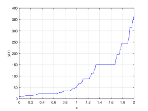
Figure 1: The graph of Eq.(15)

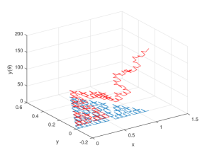
Figure 2: The graph of Eq.(16)

3 Non-local derivatives on fractals

In the following, the non-local integrals and derivatives on fractal spaces are defined [35].

3.1 Non-local derivatives of fractal sets

Definition 13.

The right-sided Riemann-Liouville $F^{\alpha}$-integral of order $\beta\in\mathbb{R}$ of $g$ (function on a fractal set) is defined by

$${}_{z}\mathcal{I}_{b}^{\beta}g(z)=\frac{1}{\Gamma(\beta)}\int_{z}^{b}\frac{g(\tau)}{(S_{\mathbf{F}}^{\alpha}(\tau)-S_{\mathbf{F}}^{\alpha}(z))^{1-\beta}}d_{\mathbf{F}}^{\alpha}\tau,$$ (17)

and the left-sided Riemann-Liouville $F^{\alpha}$-integral of $g$ is given by

$${}_{a}\mathcal{I}_{z}^{\beta}g(z)=\frac{1}{\Gamma(\beta)}\int_{a}^{z}\frac{g(\tau)}{(S_{\mathbf{F}}^{\alpha}(z)-S_{\mathbf{F}}^{\alpha}(\tau))^{1-\beta}}d_{\mathbf{F}}^{\alpha}\tau.$$ (18)

Definition 14.

The right-sided Riemann-Liouville $F^{\alpha}$-derivative of order $\beta\in\mathbb{R}$ of $g$ is defined by

$${}_{z}\mathcal{D}_{b}^{\beta}g(z)=\frac{1}{\Gamma(n-\beta)}(-D_{\mathbf{F}}^{\alpha})^{n}\int_{z}^{b}\frac{g(\tau)}{(S_{\mathbf{F}}^{\alpha}(\tau)-S_{\mathbf{F}}^{\alpha}(z))^{-n+\beta+1}}d_{\mathbf{F}}^{\alpha}\tau,\leavevmode\nobreak\ \leavevmode\nobreak\ \leavevmode\nobreak\ g\in C^{n}(\mathbf{F}),$$ (19)

and the left-sided Riemann-Liouville $F^{\alpha}$-derivative of $g$ is defined by

$${}_{a}\mathcal{D}_{z}^{\beta}g(z)=\frac{1}{\Gamma(n-\beta)}(D_{\mathbf{F}}^{\alpha})^{n}\int_{a}^{z}\frac{g(\tau)}{(S_{\mathbf{F}}^{\alpha}(z)-S_{\mathbf{F}}^{\alpha}(\tau))^{-n+\beta+1}}d_{\mathbf{F}}^{\alpha}\tau,$$ (20)

where $n\alpha-\alpha\leq\beta<\alpha n$.

Definition 15.

The right-sided Caputo $F^{\alpha}$-derivative of order $\beta\in\mathbb{R}$ of $g$ is defined by

$${}_{z}^{C}\mathcal{D}_{b}^{\beta}g(z)=\frac{1}{\Gamma(n-\beta)}\int_{z}^{b}(S_{\mathbf{F}}^{\alpha}(\tau)-S_{\mathbf{F}}^{\alpha}(z))^{n-\beta-1}(-D_{\mathbf{F}}^{\alpha})^{n}g(\tau)d_{\mathbf{F}}^{\alpha}\tau,$$ (21)

and the right-sided Caputo $F^{\alpha}$-derivative of $g$ is defined by

$${}_{a}^{C}\mathcal{D}_{z}^{\beta}g(z)=\frac{1}{\Gamma(n-\beta)}\int_{a}^{z}(S_{\mathbf{F}}^{\alpha}(z)-S_{F}^{\alpha}(\tau))^{n-\beta-1}(D_{\mathbf{F}}^{\alpha})^{n}g(\tau)d_{\mathbf{F}}^{\alpha}\tau,$$ (22)

where $n\alpha-\alpha\leq\beta<\alpha n$.

Ordinary calculus	Fractal calculus on sets	Fractal calculus on curves
$$\int_{0}^{z}\tau^{m}d\tau=\frac{1}{m+1}z^{m+1}$$	$$\int_{0}^{z}(S_{\mathbf{F}}^{\alpha}(\tau))^{m}d_{\mathbf{F}}^{\alpha}\tau=\frac{1}{m+1}(S_{\mathbf{F}}^{\alpha}(z))^{m+1}$$	$$\int_{0}^{\theta}J_{\mathfrak{F}}^{\alpha}(\tau)^{m}d_{\mathfrak{F}}^{\alpha}\tau=\frac{1}{m+1}(J(\theta))^{m+1}$$
$$\frac{d}{dz}z^{m}=mz^{m-1}$$	$$D_{\mathbf{F}}^{\alpha}(S_{\mathbf{F}}^{\alpha}(z))^{m}=m(S_{\mathbf{F}}^{\alpha}(z))^{m-1}\chi_{\mathbf{F}}(z)$$	$$D_{\mathfrak{F}}^{\alpha}(J(\theta))^{m}=m(J(\theta))^{m-1}\chi_{\mathfrak{F}}(\theta)$$
${}_{0}I_{z}^{\beta}z^{m}$ $\displaystyle=\frac{\Gamma(m+1)}{\Gamma(m+\beta+1)}z^{m+\beta}$	${}_{0}\mathcal{I}_{z}^{\beta}(S_{\mathbf{F}}^{\alpha}(z))^{m}$ $\displaystyle=\frac{\Gamma(m+1)}{\Gamma(m+\beta+1)}(S_{\mathbf{F}}^{\alpha}(z))^{m+\beta}$	${}_{0}\mathcal{I}_{\theta}^{\beta}J(\theta)^{m}$ $\displaystyle=\frac{\Gamma(m+1)}{\Gamma(m+\beta+1)}J(\theta)^{m+\beta}$
${}_{0}D_{z}^{\beta}z^{m}$ $\displaystyle=\frac{\Gamma(m+1)}{\Gamma(m-\beta+1)}z^{m-\beta}$	${}_{0}\mathcal{D}_{z}^{\beta}(S_{\mathbf{F}}^{\alpha}(z))^{m}$ $\displaystyle=\frac{\Gamma(m+1)}{\Gamma(m-\beta+1)}(S_{\mathbf{F}}^{\alpha}(z))^{m-\beta}\chi_{\mathbf{F}}(z)$	${}_{0}\mathcal{D}_{\theta}^{\beta}J(\theta)^{m}$ $\displaystyle=\frac{\Gamma(m+1)}{\Gamma(m-\beta+1)}(J(\theta))^{m-\beta}\chi_{\mathfrak{F}}(\theta)$
${}_{a}I_{z}^{\beta}(z-a)^{m}$ $\displaystyle=\frac{\Gamma(m+1)}{\Gamma(\beta+m+1)}(z-a)^{\beta+m}$	${}_{a}\mathcal{I}_{z}^{\beta}(S_{\mathbf{F}}^{\alpha}(z)-S_{\mathbf{F}}^{\alpha}(a))^{m}$ $\displaystyle=\frac{\Gamma(m+1)}{\Gamma(\beta+m+1)}(S_{\mathbf{F}}^{\alpha}(z)-S_{\mathbf{F}}^{\alpha}(a))^{\beta+m}$	${}_{a}\mathcal{I}_{\theta}^{\beta}(J(\theta)-J(a))^{m}$ $\displaystyle=\frac{\Gamma(m+1)}{\Gamma(\beta+m+1)}(J(\theta)-J(a))^{\beta+n}$
${}_{a}D^{\beta}_{z}(z-a)^{m}=$ $\displaystyle\frac{\Gamma(m+1)}{\Gamma(m-\beta+1)}(z-a)^{m-\beta}$	${}_{a}\mathcal{D}^{\beta}_{z}(S_{\mathbf{F}}^{\alpha}(z)-S_{\mathbf{F}}^{\alpha}(a))^{m}=$ $\displaystyle\frac{\Gamma(m+1)}{\Gamma(m-\beta+1)}(S_{\mathbf{F}}^{\alpha}(z)-S_{\mathbf{F}}^{\alpha}(a))^{m-\beta}$	${}_{a}\mathcal{D}^{\beta}_{\theta}(J(\theta)-J(a))^{m}=$ $\displaystyle\frac{\Gamma(m+1)}{\Gamma(m-\beta+1)}(J(\theta)-J(a))^{n-\beta}$
${}_{-\infty}I_{z}^{\beta}\exp(\lambda z)=\lambda^{\beta}\exp(\lambda z)$	${}_{-\infty}\mathcal{I}_{z}^{\beta}\exp(\lambda S_{\mathbf{F}}^{\alpha}(z))=\lambda^{\beta}\exp(\lambda S_{\mathbf{F}}^{\alpha}(z))$	${}_{-\infty}\mathcal{I}_{\theta}^{\beta}\exp(\lambda J(\theta))=\lambda^{\beta}\exp(\lambda J(\theta))$
${}_{-\infty}D_{z}^{\beta}\cos(z)=\cos\left(z+\frac{\pi}{2}\beta\right)$	${}_{-\infty}\mathcal{D}_{z}^{\beta}\cos(S_{\mathbf{F}}^{\alpha}(z))=\cos\left(S_{\mathbf{F}}^{\alpha}(z)+\frac{\pi}{2}\beta\right)$	${}_{-\infty}\mathcal{D}_{\theta}^{\beta}\cos(J(\theta))=\cos\left(J(\theta)+\frac{\pi}{2}\beta\right)$
${}_{-\infty}D_{z}^{\beta}\exp(\lambda z)=\lambda^{\beta}\exp(\lambda z)$	${}_{-\infty}\mathcal{D}_{z}^{\beta}\exp(\lambda S_{\mathbf{F}}^{\alpha}(z))=\lambda^{\beta}\exp(\lambda S_{\mathbf{F}}^{\alpha}(z))$	${}_{-\infty}\mathcal{D}_{\theta}^{\beta}\exp(\lambda J(\theta))=\lambda^{\beta}\exp(\lambda J(\theta))$

Table 1: Some analogies of fractal calculus and standard calculus.

3.2 Non-local derivatives on fractal curves

Definition 16.

The right-sided Riemann-Liouville $F^{\alpha}$-integral of order $\beta\in\mathbb{R}$ of $f$ (on a fractal curve $F$) is defined by

$${}_{\theta}\mathcal{I}_{b}^{\beta}f(\theta)=\frac{1}{\Gamma(\beta)}\int_{D(\theta,b)}\frac{f(\tau)}{(J(t)-J(\theta))^{1-\beta}}d_{\mathfrak{F}}^{\alpha}\tau,\leavevmode\nobreak\ \leavevmode\nobreak\ \leavevmode\nobreak\ \theta\in\mathfrak{F},$$ (23)

and the left-sided Riemann-Liouville $F^{\alpha}$-integral of $f$ is defined by

$$_{a}\mathcal{I}_{\theta}^{\beta}f(\theta)=\frac{1}{\Gamma(\beta)}\int_{D(a,\theta)}\frac{f(\tau)}{(J(\theta)-J(t))^{1-\beta}}d_{\mathfrak{F}}^{\alpha}\tau.$$ (24)

Definition 17.

The right-sided Riemann-Liouville $F^{\alpha}$-derivative of order $\beta\in\mathbb{R}$ of $f$ is defined by

$${}_{\theta}\mathcal{D}_{b}^{\beta}f(\theta)=\frac{1}{\Gamma(n-\beta)}(-D_{\mathfrak{F}}^{\alpha})^{n}\int_{D(\theta,b)}\frac{f(\tau)}{(J(\tau)-J(\theta))^{-n+\beta+1}}d_{\mathfrak{F}}^{\alpha}\tau,\leavevmode\nobreak\ \leavevmode\nobreak\ \leavevmode\nobreak\ f\in C^{n}(\mathfrak{F}),$$ (25)

and the left-sided Riemann-Liouville $F^{\alpha}$-derivative of $f$ is defined by

$$_{a}\mathcal{D}_{\theta}^{\beta}f(\theta)=\frac{1}{\Gamma(n-\beta)}(D_{\mathfrak{F}}^{\alpha})^{n}\int_{D(a,\theta)}\frac{f(\tau)}{(J(\theta)-J(\tau))^{-n+\beta+1}}d_{\mathfrak{F}}^{\alpha}\tau,$$ (26)

where $n\alpha-\alpha\leq\beta<\alpha n$.

Definition 18.

The right-sided Caputo $F^{\alpha}$-derivative of order $\beta\in\mathbb{R}$ of $f$ is defined by

$${}_{\theta}^{C}\mathcal{D}_{b}^{\beta}f(\theta)=\frac{1}{\Gamma(n-\beta)}\int_{D(\theta,b)}(J(\tau)-J(\theta))^{n-\beta-1}(-D_{\mathfrak{F}}^{\alpha})^{n}f(\tau)d_{\mathfrak{F}}^{\alpha}\tau,$$ (27)

and the right-sided Caputo $F^{\alpha}$-derivative of order $\beta\in\mathbb{R}$ of $f$ is defined by

$${}_{a}^{C}\mathcal{D}_{\theta}^{\beta}f(\theta)=\frac{1}{\Gamma(n-\beta)}\int_{D(a,\theta)}(J(\theta)-J(\tau))^{n-\beta-1}(D_{F}^{\alpha})^{n}f(\tau)d_{\mathfrak{F}}^{\alpha}\tau,$$ (28)

where $n\alpha-\alpha\leq\beta<\alpha n$.

Example 2.

Consider the following function on a fractal curve

$$f(\theta)=(J(\theta)-J(a))^{\nu}.$$ (29)

Then its non-local derivative is

$$_{a}\mathcal{I}_{\theta}^{\beta}(J(\theta)-J(a))^{\nu} =\frac{1}{\Gamma(\beta)}\int_{D(a,\theta)}(J(t)-J(a))^{\nu}(J(\theta)-J(t))^{\beta-1}d_{\mathfrak{F}}^{\alpha}t.$$ (30)

By the change of variable $J(t)=J(a)+\zeta(J(\theta)-J(a))$, Eq.(30), turns into

$$_{a}\mathcal{I}_{\theta}^{\beta}(J(\theta)-J(a))^{\nu} =\frac{(J(\theta)-J(a))^{\beta+\nu}}{\Gamma(\beta)}\int_{D(0,1)}(1-\zeta)^{\beta-1}\zeta^{\nu}d_{F}^{\alpha}\zeta$$

$$=\frac{B(\nu+1,\beta)}{\Gamma(\beta)}(J(\theta)-J(a))^{\beta+\nu}$$

$$=\frac{\Gamma(\nu+1)}{\Gamma(\beta+\nu+1)}(J(\theta)-J(a))^{\beta+\nu},$$ (31)

where $B(.,.)$ is the Beta function, which is defined by

$$B(\nu+1,\beta)=\int_{D(0,1)}(1-\zeta)^{\beta-1}\zeta^{\nu}d_{F}^{\alpha}\zeta=\frac{\Gamma(\nu+1)\Gamma(\beta)}{\Gamma(\nu+\beta+1)}.$$ (32)

4 Laplace transform of the fractal Riemann-Lioville differintegral

In this section, we explore the Laplace transform of fractal Riemann-Lioville differintegral [36].

Corollary 1.

Laplace transform of the fractal Riemann-Lioville integral is defined by

$$\mathcal{L}[_{0}I_{\theta}^{\beta}f(\theta)]=J(s)^{\beta}F(s),$$ (33)

where

$$F(s)=\mathcal{L}[f(\theta)]=\int_{D(0,\infty)}\exp(-J(s)J(\theta))f(\theta)d_{\mathfrak{F}}^{\alpha}\theta.$$ (34)

Corollary 2.

The Laplace transform of the fractal Riemann-Liouville derivative is defined by

$$\mathcal{L}[_{0}\mathcal{D}_{\theta}^{\beta}f(\theta)]=J(s)^{\beta}F(s)-\sum_{k=0}^{n-1}J(s)^{k}[_{0}\mathcal{D}_{\theta}^{\beta-k-1}f(\theta)]_{\theta=0},$$ (35)

where $n\alpha-\alpha\leq\beta<n\alpha$.

Remark 2.

We note that Eq.(35), for the case $n=1$, becomes

$$\mathcal{L}[_{0}\mathcal{D}_{\theta}^{\beta}f(\theta)]=J(s)^{\beta}F(s)-\leavevmode\nobreak\ _{0}\mathcal{D}_{\theta}^{\beta-1}f(\theta)|_{\theta=0},\leavevmode\nobreak\ \leavevmode\nobreak\ \leavevmode\nobreak\ 0\leq\beta<\alpha,$$ (36)

and for $n=2$, it follows from Eq.(35) that

$$\mathcal{L}[_{0}\mathcal{D}_{\theta}^{\beta}f(\theta)]=J(s)^{\beta}F(s)-\leavevmode\nobreak\ _{0}\mathcal{D}_{\theta}^{\beta-1}f(\theta)|_{\theta=0}-J(s)_{0}\mathcal{D}_{\theta}^{\beta-2}f(\theta)|_{\theta=0},\leavevmode\nobreak\ \leavevmode\nobreak\ \leavevmode\nobreak\ \alpha\leq\beta<2\alpha.$$ (37)

Theorem 1.

The fractal Laplace transform of function $J(\theta)^{\eta m+\mu-1}E^{m}_{\eta,\mu}(aJ(\theta)^{\eta})$ is

$$\mathcal{L}[J(\theta)^{\eta m+\mu-1}E^{m}_{\eta,\mu}(aJ(\theta)^{\eta})]=\frac{m!J(s)^{\eta-\mu}}{(J(s)^{\eta}-a)^{m+1}},$$ (38)

where

$$E^{m}_{\eta,\mu}(aJ(\theta)^{\eta})=\sum_{k=0}^{\infty}\frac{(k+m)!}{k!}\frac{a^{k}J(\theta)^{k\eta}}{\Gamma(\eta k+\eta m+\mu)}.$$ (39)

Proof.

Using the linearity of the fractal Laplace transform and Eq.(39), we can rewrite Eq.(38) as

$$\mathcal{L}[J(\theta)^{\eta m+\mu-1}E^{m}_{\eta,\mu}(aJ(\theta)^{\eta})]=\sum_{k=0}^{\infty}\frac{(k+m)!a^{k}}{k!\Gamma(\eta k+\eta m+\mu)}\mathcal{L}[J(\theta)^{\eta k+\eta m+\mu-1}].$$ (40)

Applying the fractal Laplace transform of the power function $\mathcal{L}[J(\theta)^{\beta-1}]=\Gamma(\beta)J(s)^{-\beta}$, Eq.(40) turns into the following form

$$\mathcal{L}[J(\theta)^{\eta m+\mu-1}E^{m}_{\eta,\mu}(aJ(\theta)^{\eta})] =\sum_{k=0}^{\infty}\frac{(k+m)!a^{k}}{k!\Gamma(\eta k+\eta m+\mu)}\frac{\Gamma(\eta k+\eta m+\mu)}{J(s)^{\eta k+\eta m+\mu}}$$

$$=\sum_{k=0}^{\infty}\frac{(k+m)!}{k!}\frac{a^{k}}{J(s)^{\eta k+\eta m+\mu}}$$

$$=J(s)^{-\eta m-\mu}\sum_{k=0}^{\infty}\frac{(k+m)!}{k!}\bigg{(}\frac{a}{J(s)^{\eta}}\bigg{)}^{k}$$

$$=J(s)^{-\eta m-\mu}D_{\mathfrak{F}}^{m}\sum_{k=m}^{\infty}\bigg{(}\frac{a}{J(s)^{\eta}}\bigg{)}^{k}$$

$$=J(s)^{-\eta m-\mu}D_{\mathfrak{F}}^{m}\frac{1}{(1-\frac{a}{J(s)^{\eta}})}$$

$$=J(s)^{-\eta m-\mu}\frac{m!}{(1-\frac{a}{J(s)^{\eta}})^{m+1}}$$

$$=\frac{m!J(s)^{\eta-\mu}}{(J(s)^{\eta}-a)^{m+1}},$$ (41)

which completes the proof. ∎

Function in $\theta$-space	Fractal Laplace Transform $s$-space
$$\frac{J(\theta)^{\beta-1}}{\Gamma(\beta)}$$	$$\frac{1}{J(s)^{\beta}}$$
$$J(\theta)^{\beta-1}E_{\beta,\beta}(aJ(\theta)^{\beta})$$	$$\frac{1}{J(s)^{\beta}-a}$$
$$E_{\beta}(-aJ(\theta)^{\beta})$$	$$\frac{J(s)^{\beta}}{J(s)(J(s)^{\beta}+a)}$$
$$1-E_{\beta}(-aJ(\theta)^{\beta})$$	$$\frac{a}{J(s)(J(s)^{\beta}+a)}$$
$$J(\theta)^{\beta}E_{1,\beta+1}(aJ(\theta))$$	$$\frac{1}{J(s)^{\beta}(J(s)-a)}$$
$$J(\theta)^{\beta-1}E_{\nu,\beta}(aJ(\theta)^{\nu})$$	$$\frac{J(s)^{\nu-\beta}}{(J(s)^{\nu}-a)}$$
$$J(\theta)^{\eta m+\mu-1}E^{m}_{\eta,\mu}(aJ(\theta)^{\eta})$$	$$\frac{m!J(s)^{\eta-\mu}}{(J(s)^{\eta}-a)^{m+1}}$$

Table 2: Some formulas of the fractal Laplace transforms.

Corollary 3.

The Laplace transform of the Caputo derivative is defined by

$$\mathcal{L}[_{0}^{C}\mathcal{D}_{\theta}^{\beta}f(\theta)]=J(s)^{\beta}F(s)-\sum_{k=0}^{n-1}J(s)^{\beta-k-1}[(D_{\mathfrak{F}}^{\alpha})^{k}f(\theta)]_{\theta=0},$$ (42)

where $n\alpha-\alpha<\beta\leq n\alpha$.

Example 3.

Consider the non-local fractal differential equation

$$_{0}D_{\theta}^{\beta}y(\theta)-\lambda y(\theta)=h(\theta),\leavevmode\nobreak\ \leavevmode\nobreak\ (\theta>0),$$ (43)

with the non-local initial condition

$$[_{0}D_{\theta}^{\beta-k}y(\theta)]_{\theta=0}=c_{k},\leavevmode\nobreak\ \leavevmode\nobreak\ \leavevmode\nobreak\ (k=1,2,...,n),$$ (44)

where $n\alpha-\alpha\leq\beta<n\alpha$ and $\lambda$ is constant.
To solve this problem, taking the fractal non-local Laplace transform of Eq.(43) and using Eq.(35) we obtain

$$J(s)^{\beta}Y(J(s))-\lambda Y(J(s))=H(J(s))+\sum_{k=1}^{n}c_{k}J(s)^{k-1}.$$ (45)

Solving for $Y(J(s))$, we have

$$Y(J(s))=\frac{H(J(s))}{J(s)^{\beta}-\lambda}+\sum_{k=1}^{n}c_{k}\frac{J(s)^{k-1}}{J(s)^{\beta}-\lambda}.$$ (46)

The fractal inverse Laplace transform and Eq.(38) give the solution

$$y(\theta)=\sum_{k=1}^{n}c_{k}J(\theta)^{\beta-k}E_{\beta,\beta-k+1}(\lambda J(\theta)^{\beta})+\int_{D(0,\theta)}(J(\theta)-J(t))^{\beta-1}E_{\beta,\beta}(\lambda(J(\theta)-J(t))^{\beta})h(t)d_{\mathfrak{F}}^{\alpha}t.$$ (47)

5 The analogue of Mellin integral transform on fractal calculus

In this section, we generalize the Mellin integral transform to include a function with fractal support.

Definition 19.

The Mellin integral transform $M(s)$ of a function $f$ on fractals is defined by

$$M(s)=\int_{D(0,\infty)}f(\theta)J(\theta)^{J(s)-1}d_{\mathfrak{F}}^{\alpha}\theta,$$ (48)

where $J(s)$ is complex, such as $\lambda_{1}<Re(J(s))<\lambda_{2}$. The Mellin transform exists if $f$ is fractal piecewise continuous in every closed interval $D(a,b)\subset D(0,\infty)$ and

$$\int_{D(0,1)}|f(\theta)|J(\theta)^{\lambda_{1}-1}d_{\mathfrak{F}}^{\alpha}\theta<\infty,\leavevmode\nobreak\ \leavevmode\nobreak\ \leavevmode\nobreak\ \int_{D(1,\infty)}|f(\theta)|J(\theta)^{\lambda_{2}-1}d_{\mathfrak{F}}^{\alpha}\theta<\infty.$$ (49)

Definition 20.

The fractal inverse Mellin transform formula is defined by

$$f(\theta)=\frac{1}{2\pi i}\int_{\lambda-i\infty}^{\lambda+i\infty}M(z)J(\theta)^{-z}dz,\leavevmode\nobreak\ \leavevmode\nobreak\ \leavevmode\nobreak\ (0<J(\theta)<\infty),$$ (50)

where $\lambda_{1}<\lambda<\lambda_{2}$.

Example 4.

The fractal Mellin transform of function $J(\theta)^{\nu}f(\theta)$ is

$$\mathcal{M}(J(\theta)^{\nu}f(\theta))=\int_{D(0,\infty)}J(\theta)^{\nu}f(\theta)J(\theta)^{J(s)-1}d_{\mathfrak{F}}^{\alpha}\theta=M(\nu+J(s)).$$ (51)

Definition 21.

The fractal Mellin convolution is defined by

$$f(\theta)*h(\theta)=\int_{D(0,\infty)}f(J(\theta)\tau)h(\tau)d_{\mathfrak{F}}^{\alpha}\tau,$$ (52)

and its fractal Mellin transform is

$$\mathcal{M}\{f(J(\theta)\tau)g(\tau)d_{\mathfrak{F}}^{\alpha}\tau\}=M_{1}(J(s))M_{2}(1-J(s)),$$ (53)

where $M_{1}(.)$ and $M_{2}(.)$ are the fractal Mellin transform of $f(\theta)$ and $h(\theta)$, respectively.

Corollary 4.

The fractal Mellin transform holds

$$\mathcal{M}\bigg{[}J(\theta)^{\kappa}\int_{D(0,\infty)}J(t)^{\tau}f(J(\theta)t)g(t)d_{\mathfrak{F}}^{\alpha}t\bigg{]}=M_{1}(J(s)+\kappa)M_{2}(1-J(s)-\kappa+\tau).$$ (54)

Theorem 2.

The fractal Mellin transform of $n$-th $F^{\alpha}$-derivative is

$$\mathcal{M}[(D_{\mathfrak{F}}^{\alpha})^{n}f(\theta)]=\frac{\Gamma(1-J(s)+n)}{\Gamma((1-J(s))}M(J(s)-n).$$ (55)

Proof.

To prove of this theorem, we use the fractal integral by part as follows

$$\mathcal{M}[(D_{\mathfrak{F}}^{\alpha})^{n}f(\theta)] =\int_{D(0,\infty)}(D_{\mathfrak{F}}^{\alpha})^{n}f(\theta)J(\theta)^{J(s)-1}d_{\mathfrak{F}}^{\alpha}\theta$$

$$=[(D_{\mathfrak{F}}^{\alpha})^{n-1}f(\theta)J(\theta)^{J(s)-1}\bigg{|}_{0}^{\infty}-(J(s)-1)\int_{D(0,\infty)}D_{\mathfrak{F}}^{\alpha})^{n-1}f(\theta)J(\theta)^{J(s)-2}d_{\mathfrak{F}}^{\alpha}\theta$$

$$=[(D_{\mathfrak{F}}^{\alpha})^{n-1}f(\theta)J(\theta)^{J(s)-1}\bigg{|}_{0}^{\infty}-(J(s)-1)\mathcal{M}[(D_{\mathfrak{F}}^{\alpha})^{n-1}f(\theta)]$$

$$=...$$

$$=\sum_{k=0}^{n-1}(-1)^{k}\frac{\Gamma(J(s))}{\Gamma(J(s)-k)}[D_{\mathfrak{F}}^{\alpha})^{n-k-1}f(\theta)J(\theta)^{J(s)-k-1}\bigg{|}_{0}^{\infty}+(-1)^{n}\frac{\Gamma(J(s))}{\Gamma(J(s)-k)}M(J(s)-n)$$

$$=\sum_{k=0}^{n-1}\frac{\Gamma(1-J(s)+k)}{\Gamma(1-J(s))}[D_{\mathfrak{F}}^{\alpha})^{n-k-1}f(\theta)J(\theta)^{J(s)-k-1}\bigg{|}_{0}^{\infty}+\frac{\Gamma(1-J(s)+n)}{\Gamma(1-J(s))}M(J(s)-n).$$ (56)

The first term of the right side of Eq.(5) as the limits $t=0$ and $t=\infty$ is zero. Then Eq.(5) takes the form

$$\mathcal{M}[(D_{\mathfrak{F}}^{\alpha})^{n}f(\theta)]=\frac{\Gamma(1-J(s)+n)}{\Gamma(1-J(s))}M(J(s)-n),$$ (57)

which completes the proof. ∎

Theorem 3.

The Mellin transform of the fractal Riemann-Liouville is

$$\mathcal{M}[_{0}\mathcal{I}_{\theta}^{\beta}f(\theta)]=\frac{\Gamma(1-J(s)-\beta)}{\Gamma(1-J(s))}M(J(s)+\beta),$$ (58)

where $M(J(s))$ is the Mellin transform of the function $f(J(\theta))$.

Proof.

To prove this theorem, recalling the Definition 24 and setting $a=0$ we have

$$_{0}\mathcal{I}_{\theta}^{\beta}f(\theta) =\frac{1}{\Gamma(\beta)}\int_{D(0,\theta)}(J(\theta)-J(t))^{\beta-1}f(t)d_{\mathfrak{F}}^{\alpha}t,$$

by setting $$J(t)=J(\theta)\zeta$$ we have

$${}_{0}\mathcal{I}_{\theta}^{\beta}f(\theta) =\frac{J(\theta)^{\beta}}{\Gamma(\beta)}\int_{D(0,1)}(1-\zeta)^{\beta-1}f(J(\theta)\zeta)d_{\mathfrak{F}}^{\alpha}\zeta\leavevmode\nobreak\ \leavevmode\nobreak\ \leavevmode\nobreak\$$

$$=\frac{J(\theta)^{\beta}}{\Gamma(\beta)}\int_{D(0,\infty)}f(J(\theta)\zeta)h(\zeta)d_{\mathfrak{F}}^{\alpha}\zeta,$$ (59)

where

$$h(\theta)=\left\{\begin{array}[]{ll}(1-\theta)^{\beta-1},&(0\leq\theta<1);\\ 0,&(\theta\geq 1).\end{array}\right.$$ (60)

The fractal Mellin transform of $h(\theta)$ is

$$\mathcal{M}[h(\theta)]=B(\beta,J(s))=\frac{\Gamma(\beta)\Gamma(J(s))}{\Gamma(\beta+J(s))},$$ (61)

where $B(.,.)$ is the Beta function. Using Corollary 4, Eq.(5) and Eq.(61), we have

$$\mathcal{M}[_{0}\mathcal{I}_{\theta}^{\beta}f(\theta)]=\frac{1}{\Gamma(\beta)}M(J(s)+\beta)B(\beta,1-J(s)-\beta),$$ (62)

or

$$\mathcal{M}[_{0}\mathcal{I}_{\theta}^{\beta}f(\theta)]=\frac{\Gamma(1-J(s)-\beta)}{\Gamma(1-J(s))}M(J(s)+\beta),$$ (63)

which completes the proof. ∎

Theorem 4.

The fractal Mellin transform of the Riemann-Liouville derivative is

$$\mathcal{M}[_{0}\mathcal{D}_{\theta}^{\beta}f(\theta)]=\frac{\Gamma(1-J(s)-\beta)}{\Gamma(1-J(s))}M(J(s)-\beta).$$ (64)

Proof.

By view of Definitions 26 and 19, we have

$$\mathcal{M}[_{0}\mathcal{D}_{\theta}^{\beta}f(\theta)] =\mathcal{M}[(D_{F}^{\alpha})^{n}\leavevmode\nobreak\ _{0}\mathcal{D}_{\theta}^{\beta-n}f(\theta)],$$ (65)

and setting $h(\theta)=\leavevmode\nobreak\ _{0}\mathcal{D}_{\theta}^{-(n-\beta)}f(\theta)$ we have

$$\mathcal{M}[_{0}\mathcal{D}_{\theta}^{\beta}f(\theta)]=\mathcal{M}[(D_{F}^{\alpha})^{n}h(\theta)].$$ (66)

Recalling Theorem 2, we can write

$$\mathcal{M}[(D_{\mathfrak{F}}^{\alpha})^{n}h(\theta)] =\sum_{k=0}^{n-1}\frac{\Gamma(1-J(s)+k)}{\Gamma(1-J(s))}[D_{\mathfrak{F}}^{\alpha})^{n-k-1}h(\theta)J(\theta)^{J(s)-k-1}\bigg{|}_{0}^{\infty}+\frac{\Gamma(1-J(s)+n)}{\Gamma(1-J(s))}H(J(s)-n),$$ (67)

where $H(J(s))$ is the fractal Mellin transform of $h(J(\theta))$. By replacing $h(\theta)$, we rewrite Eq.(67) as

$$\mathcal{M}[_{0}\mathcal{D}_{\theta}^{\beta}f(\theta)] =\sum_{k=0}^{n-1}\frac{\Gamma(1-J(s)+k)}{\Gamma(1-J(s))}[D_{\mathfrak{F}}^{\alpha})^{n-k-1}\leavevmode\nobreak\ _{0}\mathcal{D}_{\theta}^{-(n-\beta)}f(\theta)J(\theta)^{J(s)-k-1}\bigg{|}_{0}^{\infty}$$

$$+\frac{\Gamma(1-J(s)+n)}{\Gamma(1-J(s))}\frac{\Gamma(1-(J(s)-n)-(n-\beta))}{\Gamma(1-(J(s)-n))}M((J(s)-n)+(n-\beta)),$$ (68)

or

$$\mathcal{M}[_{0}\mathcal{D}_{\theta}^{\beta}f(\theta)] =\sum_{k=0}^{n-1}\frac{\Gamma(1-J(s)+k)}{\Gamma(1-J(s))}[_{0}\mathcal{D}_{\theta}^{\beta-k-1}f(\theta)J(\theta)^{J(s)-k-1}\bigg{]}_{0}^{\infty}+\frac{\Gamma(1-J(s)+\beta)}{\Gamma(1-J(s))}M(J(s)-\beta).$$ (69)

In the case of $1<\beta<\alpha$, Eq.(69) turns into

$$\mathcal{M}[_{0}\mathcal{D}_{\theta}^{\beta}f(\theta)] =\leavevmode\nobreak\ _{0}\mathcal{D}_{\theta}^{\beta-1}f(\theta)J(\theta)^{J(s)-1}\bigg{]}_{0}^{\infty}+\frac{\Gamma(1-J(s)+\beta)}{\Gamma(1-J(s))}M(J(s)-\beta).$$ (70)

By substituting the limits $\theta=0$ and $\theta=\infty$, the first term of right side of Eq.(70) is zero, and Eq.(70) on the simplest becomes

$$\mathcal{M}[_{0}\mathcal{D}_{\theta}^{\beta}f(\theta)]=\frac{\Gamma(1-J(s)+\beta)}{\Gamma(1-J(s))}M(J(s)-\beta).$$ (71)

∎

Theorem 5.

The fractal Mellin transform of the Caputo derivative is

$$\mathcal{M}[_{0}^{C}\mathcal{D}_{\theta}^{\beta}f(\theta)]=\frac{\Gamma(1-J(s)+\beta)}{\Gamma(1-J(s))}M(J(s)-\beta).$$ (72)

Proof.

For proving this theorem, by virtue of Definition 19 we have

$$\mathcal{M}[_{0}^{C}\mathcal{D}_{\theta}^{\beta}f(\theta)]=\mathcal{M}[_{0}\mathcal{D}_{\theta}^{-(n-\beta)}(D_{\mathfrak{F}}^{\alpha})^{n}f(\theta)].$$ (73)

By supposing $h(\theta)=(D_{\mathfrak{F}}^{\alpha})^{n}f(\theta)$ we get

$$\mathcal{M}[_{0}^{C}\mathcal{D}_{\theta}^{\beta}f(\theta)] =\mathcal{M}[_{0}\mathcal{D}_{\theta}^{-(n-\beta)}h(\theta)]$$

$$=\frac{1-J(s)-(n-\beta)}{\Gamma(1-J(s))}H(J(s)+(n+\beta))$$

$$=\frac{\Gamma(1-J(s)-n+\beta))}{\Gamma(1-J(s))}\bigg{\{}\sum_{k=0}^{n-1}\frac{\Gamma(1-(J(s)+n-\beta)+k)}{\Gamma(1-(J(s)+n-\beta))}\bigg{[}(D_{\mathfrak{F}}^{\alpha})^{n-k-1}f(\theta)J(\theta)^{(J(s)+n-\beta)-k-1}\bigg{]}_{0}^{\infty}$$

$$+\frac{\Gamma(1-(J(s)+n-\beta)+n)}{\Gamma(J(s)+n-\beta-n)}M((J(s)+n-\beta)-n)\bigg{\}}$$

$$=\sum_{k=0}^{n-1}\frac{\Gamma(1-J(s)-n+\beta+k)}{\Gamma(1-J(s))}\bigg{[}(D_{\mathfrak{F}}^{\alpha})^{n-k-1}f(\theta)J(\theta)^{J(s)+n-\beta-k-1}\bigg{]}_{0}^{\infty}$$

$$+\frac{\Gamma(1-J(s)-\beta)}{\Gamma(1-J(s))}M(J(s)-\beta),$$ (74)

or

$$\mathcal{M}[_{0}^{C}\mathcal{D}_{\theta}^{\beta}f(\theta)] =\sum_{k=0}^{n-1}\frac{\Gamma(\beta-n-J(s))}{\Gamma(1-J(s))}\bigg{[}(D_{\mathfrak{F}}^{\alpha})^{k}f(\theta)J(\theta)^{J(s)-\beta+k}\bigg{]}_{0}^{\infty}$$

$$+\frac{\Gamma(1-J(s)-\beta)}{\Gamma(1-J(s))}M(J(s)-\beta).$$ (75)

For the case of $1<\beta<\alpha$, Eq.(5) turn into

$$\mathcal{M}[_{0}^{C}\mathcal{D}_{\theta}^{\beta}f(\theta)]=\frac{\Gamma(\beta-J(s))}{\Gamma(1-J(s))}\bigg{[}f(\theta)J(\theta)^{J(s)-\beta}\bigg{]}_{0}^{\infty}+\frac{\Gamma(1-J(s)-\beta)}{\Gamma(1-J(s))}M(J(s)-\beta).$$ (76)

By taking into account of the limits $\theta=0$ and $\theta=\infty$, we arrive at

$$\mathcal{M}[_{0}^{C}\mathcal{D}_{\theta}^{\beta}f(\theta)]=\frac{\Gamma(1-J(s)-\beta)}{\Gamma(1-J(s))}M(J(s)-\beta).$$ (77)

Then the proof is complete. ∎

Example 5.

Consider the fractal differential equation

$$D_{\mathfrak{F}}^{\alpha}f(\theta)+f(\theta)=0,$$ (78)

By taking the fractal Mellin transform we have

$$-(J(s)-1)M(J(s)-1)+M(J(s))=0\leavevmode\nobreak\ \leavevmode\nobreak\ \leavevmode\nobreak\ \textmd{or}\leavevmode\nobreak\ \leavevmode\nobreak\ \leavevmode\nobreak\ M(J(s)-1)=J(s)M(J(s)).$$ (79)

The solution of Eq.(79) is $M(J(s))=\Gamma(J(s))$. Then the fractal inverse Mellin transform gives the solution of Eq.(78) by

$$f(\theta) =\frac{1}{2\pi i}\int_{c-i\infty}^{c+i\infty}J(\theta)^{-z}\Gamma(z)d_{\mathfrak{F}}^{\alpha}z$$

$$=\sum_{n=0}^{\infty}Res_{z=-n}J(s)^{-z}\Gamma(z)$$

$$=\sum_{n=0}^{\infty}J(s)^{n}\frac{(-1)^{n}}{n!}=\exp(-J(\theta)).$$ (80)

6 Conclusion

In this paper, the Riemann-Liouville integrals and derivatives and Caputo derivatives of fractal sets and curves have been defined. The processes on fractal spaces with memory effect can be modeled by them. Fractal differential equations have been solved by using the Mellin transform. The solution of the fractal differential equation is not differentiable in the standard calculus. The results become standard cases if we choose $\alpha=1$.

7 Appendix

In this section, we give some formulas used in the paper [37, 38].
The Mittag-Leffler one-parameter function is defined by

$$E_{\alpha}(x)=\sum_{k=0}^{\infty}\frac{x^{k}}{\Gamma(\alpha k+1)},\leavevmode\nobreak\ \leavevmode\nobreak\ (\alpha>0,\leavevmode\nobreak\ \leavevmode\nobreak\ \beta>0).$$ (81)

The Mittag-Leffler two-parameter function is defined by

$$E_{\alpha,\beta}(x)=\sum_{k=0}^{\infty}\frac{x^{k}}{\Gamma(\alpha k+\beta)},\leavevmode\nobreak\ \leavevmode\nobreak\ (\alpha>0,\leavevmode\nobreak\ \leavevmode\nobreak\ \beta>0),$$ (82)

where $E_{\alpha,1}(x)=E_{\alpha}(x)$.
The gamma function is defined by

$$\Gamma(x)=\int_{0}^{\infty}e^{-\tau}\tau^{x-1}d\tau.$$ (83)

The beta function is defined by

$$\mathbf{B}(x,\nu)=\int_{0}^{1}\tau^{x-1}(1-\tau)^{\nu-1}d\tau,\leavevmode\nobreak\ \leavevmode\nobreak\ \leavevmode\nobreak\ (Re(x)>0,\leavevmode\nobreak\ \leavevmode\nobreak\ Re(\nu)>0).$$ (84)

The beta function relates to the gamma function by the following equation

$$\mathbf{B}(x,\nu)=\frac{\Gamma(x)\Gamma(\nu)}{\Gamma(x+\nu)}.$$ (85)

Acknowledgements: Cristina Serpa acknowledges partial funding by national funds through FCT-Foundation for Science and Technology, project reference: UIDB/04561/2020.

References

• [1] B. B. Mandelbrot, The Fractal Geometry of Nature, WH freeman New York, 1982.
• [2] M. F. Barnsley, Fractals Everywhere, Academic Press, 2014.
• [3] K. J. Falconerm, Fractal Geometry: Mathematical Foundations and Applications, John Wiley & Sons, 2004.
• [4] G. A. Edgar, Integral, Probability, and Fractal Measures, Springer New York, 1998.
• [5] M. L. Lapidus, G. Radunović, D. Žubrinić, Fractal Zeta Functions and Fractal Drums, Springer International Publishing, 2017.
• [6] M. Khelifi, H. Lotfi, A. Samti, B. Selmi, A relative multifractal analysis, Chaos, Solitons & Fractals 140 (2020) 110091.
• [7] J. Kigami, Analysis on Fractals, Cambridge University Press, 2001.
• [8] R. S. Strichartz, Differential Equations on Fractals, Princeton University Press, 2018.
• [9] U. Freiberg, M. Zähle, Harmonic calculus on fractals-a measure geometric approach I, Potential Anal. 16 (3) (2002) 265–277.
• [10] M. T. Barlow, E. A. Perkins, Brownian motion on the Sierpinski gasket, Probab. Theory Rel. 79 (4) (1988) 543–623.
• [11] F. H. Stillinger, Axiomatic basis for spaces with noninteger dimension, J. Math. Phys. 18 (6) (1977) 1224–1234.
• [12] V. E. Tarasov, Fractional Dynamics, Springer Berlin Heidelberg, 2010.
• [13] L. Nottale, J. Schneider, Fractals and nonstandard analysis, J. Math. Phys. 25 (5) (1984) 1296–1300.
• [14] C. Serpa, Affine fractal least squares regression model, Fractals 30 (7) (2022) 2250138.
• [15] A. Parvate, A. D. Gangal, Calculus on fractal subsets of real line-I: Formulation, Fractals 17 (01) (2009) 53–81.
• [16] A. Parvate, S. Satin, A. Gangal, Calculus on fractal curves in Rn, Fractals 19 (01) (2011) 15–27.
• [17] A. Parvate, A. Gangal, Calculus on fractal subsets of real line-II: Conjugacy with ordinary calculus, Fractals 19 (03) (2011) 271–290.
• [18] A. K. Golmankhaneh, Fractal Calculus and its Applications, World Scientific, 2022.
• [19] R. A. El-Nabulsi, A. K. Golmankhaneh, On fractional and fractal Einstein’s field equations, Mod. Phys. Lett. A 36 (05) (2021) 2150030.
• [20] A. K. Golmankhaneh, K. Welch, Equilibrium and non-equilibrium statistical mechanics with generalized fractal derivatives: A review, Mod. Phys. Lett. A 36 (14) (2021) 2140002.
• [21] A. K. Golmankhaneh, C. Cattani, Fractal logistic equation, Fractal Fract. 3 (3) (2019) 41.
• [22] A. K. Golmankhaneh, A. Fernandez, Random variables and stable distributions on fractal Cantor sets, Fractal Fract. 3 (2) (2019) 31.
• [23] R. Banchuin, Nonlocal fractal calculus based analyses of electrical circuits on fractal set, COMPEL - Int. J. Comput. Math. Electr. Electron. Eng. 41 (1) (2022) 528–549.
• [24] R. Banchuin, Noise analysis of electrical circuits on fractal set, COMPEL - Int. J. Comput. Math. Electr. Electron. Eng. 41 (5) (2022) 1464–1490.
• [25] A. K. Golmankhaneh, On the fractal Langevin equation, Fractal Fract. 3 (1) (2019) 11.
• [26] A. K. Golmankhaneh, R. T. Sibatov, Fractal stochastic processes on thin Cantor-like sets, Mathematics 9 (6) (2021) 613.
• [27] A. K. Golmankhaneh, A. S. Balankin, Sub-and super-diffusion on Cantor sets: Beyond the paradox, Phys. Lett. A. 382 (14) (2018) 960–967.
• [28] A. K. Golmankhaneh, C. Tunç, Sumudu transform in fractal calculus, Appl. Math. Comput. 350 (2019) 386–401.
• [29] A. K. Golmankhaneh, C. Tunç, H. Şevli, Hyers–Ulam stability on local fractal calculus and radioactive decay, Eur. Phys. J. Special Topics 230 (21) (2021) 3889–3894.
• [30] F. A. Cetinkaya, A. K. Golmankhaneh, General characteristics of a fractal Sturm-Liouville problem, Turk. J. Math. 45 (4) (2021).
• [31] A. K. Golmankhaneh, K. K. Ali, R. Yilmazer, M. K. A. Kaabar, Local fractal fourier transform and applications, Comput. Methods Differ. Equ., doi 10 (2021).
• [32] A. K. Golmankhaneh, A. Fernandez, Fractal calculus of functions on Cantor tartan spaces, Fractal Fract. 2 (4) (2018) 30.
• [33] A. K. Golmankhaneh, S. M. Nia, Laplace equations on the fractal cubes and Casimir effect, Eur. Phys. J. Special Topics 230 (21) (2021) 3895–3900.
• [34] A. Gowrisankar, A. K. Golmankhaneh, C. Serpa, Fractal calculus on fractal interpolation functions, Fractal Fract. 5 (4) (2021) 157.
• [35] A. K. Golmankhaneh, D. Baleanu, Non-local integrals and derivatives on fractal sets with applications, Open Physics 14 (1) (2016) 542–548.
• [36] A. K. Kamal, A. K. Golmankhaneh, R. Yilmazer, M. A. Abdullah, Solving fractal differential equations via fractal Laplace transforms, J. Appl. Anal. 28 (2) (2022) 237–250.
• [37] T. Sandev, Ž. Tomovski, Fractional Equations and Models: Theory and Applications, Springer, 2020.
• [38] I. Podlubny, Fractional differential equations: an introduction to fractional derivatives, fractional differential equations, to methods of their solution and some of their applications, Elsevier, 1998.