Cox reduction and confidence sets of models: a theoretical elucidation

Abstract

For sparse high-dimensional regression problems, Cox and Battey [1, 9] emphasised the need for confidence sets of models: an enumeration of those small sets of variables that fit the data equivalently well in a suitable statistical sense. This is to be contrasted with the single model returned by penalised regression procedures, effective for prediction but potentially misleading for subject-matter understanding. The proposed construction of such sets relied on preliminary reduction of the full set of variables, and while various possibilities could be considered for this, [9] proposed a succession of regression fits based on incomplete block designs. The purpose of the present paper is to provide insight on both aspects of that work. For an unspecified reduction strategy, we begin by characterising models that are likely to be retained in the model confidence set, emphasising geometric aspects. We then evaluate possible reduction schemes based on penalised regression or marginal screening, before theoretically elucidating the reduction of [9]. We identify features of the covariate matrix that may reduce its efficacy, and indicate improvements to the original proposal. An advantage of the approach is its ability to reveal its own stability or fragility for the data at hand.

1 Introduction

In the context of regression with a large number of potential explanatory features, usual practice is to identify a single low-dimensional model. Motivated by scientific studies in which subject-matter understanding is sought rather than immediate predictive success, [9] argued that when several alternative reasonable explanations are statistically indistinguishable, one should aim to specify as many as is feasible, aiming for a confidence set of models. The arguments for this are in our view overwhelming, yet there may be some flexibility in how the broad goal is operationalised. The following procedure was proposed in [9].

If, among the potential explanatory variables, some have inordinately high sample correlation ($>0.97$ say), the variables are temporarily paired, with one representative of both. Depending on the magnitude $p$ of the resulting set of variables, the associated variable indices are arranged in a $k\times k$ square, $k\times k\times k$ cube, or higher dimensional array (hypercube). There is no need for $p$ to be a perfect cube etc., as some entries of the array can be left empty. We describe the cubic case for concreteness.

The rows, columns and tube fibres of the cube are successively traversed, and the outcome variable is regressed on the corresponding set of $k$ variables. Thus, among the $3k^{2}$ regressions that are run, each variable appears three times, each time with a different set of $k-1$ companion variables. In other words, this is a partially balanced incomplete block arrangement, as proposed by Yates [38] in the context of agricultural field trials. Figure 1 depicts this arrangement for $p=1000$ variables. Any intrinsic biological or physiological characteristics, known to be important, are either used to partition the sample or are included in all regressions and should not be arranged in the cube. Variables are retained if they are among the two most significant in at least two of the three regressions in which they appear. If the number of retained variables exceeds or is close to the sample size, the procedure is repeated, arranging the indices of the retained variables in a square or, more generally, a hypercube of lower dimension than in the previous stage. As before, a regression is fitted to each set and variables are retained if they are significant at some threshold in at least half the regressions in which they appear. The threshold to be chosen is such that a fairly large but not unmanageable number of variables are retained, certainly fewer than the sample size, and that the set of retained variables exhibits stability under rerandomisation of the variable indices in the cube. The final set of variables, $\hat{\mathcal{S}}$ say, is called the comprehensive model.

Other decision rules for retaining variables were studied under idealised conditions in [1] and the above was found to be optimal. We refer henceforth to this version of backwards elimination based on incomplete block designs as Cox reduction. Any variables that were paired through this procedure are unpaired if the representative variable survives.

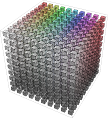
Figure 1: Partially balanced incomplete block arrangement of $p=1000$ variables in blocks of size $k=10$. Each small cube represents a variable index and appears with $k-1$ companion variables. The colour is for visualisation only and plays no role in the analysis.

The next stage of the procedure, emphasised by [9] but ignored in the present paper, is an exploratory phase, aiming to identify possible interactions and other nonlinearities among the variables.

Finally, a confidence set of models $\mathcal{M}$ is constructed as all those small sets of variables for which a likelihood ratio test against the comprehensive model fails to reject at a chosen significance level. The sample needs to be split for use in alternating phases of the analysis, an aspect to which we return in subsequent sections.

Motivation for Cox reduction comes from Bradford Hill’s [2] discussion of the circumstances under which an effect obtained in an observational study is relatively likely to have a causal interpretation. Such conditions include that the effect is reproduced in independent studies and behaves appropriately when the potential cause is applied, removed and then reinstated [8]. See [10, p.165–6] for further discussion. Cox reduction analyses variables alongside different sets of companion variables and those whose apparent effects are not explained away by other variables are retained for more detailed joint analysis. For a different approach with a somewhat similar motivation, see [29].

A practical advantage of Cox reduction is the reassurance it offers, through rerandomisation of the variable indices in the cube, over the security or otherwise of the conclusions. In particular, unstable sets $\hat{\mathcal{S}}$ point to fragility of the method on the data at hand and thereby guide the choice of tuning parameters.

In a low-dimensional context, confidence sets of models have been emphasised repeatedly by Cox (see e.g., [7], [11], [12, Appendix A.2.5]). They have also been considered from a different perspective in [25]. The authors of the latter paper begin with a collection of candidate models and aim to identify those with the smallest expected loss at a given significance level. In [25], the relative explanatory power of pairs of models in the candidate set are compared, whereas [9] uses the comprehensive model as a reference set against which to gauge the adequacy of each submodel. If no submodel achieves comparable fit, the model confidence set of [9] is empty, whereas the set of [25] contains several models with equally poor fit.

The present paper provides insight into the efficacy of Cox reduction and the proposed confidence set of models, revealing situations that lead the procedure to partially fail, either by discarding a genuinely relevant variable (a signal variable) in the reduction phase, or by discarding the true model at the model assessment phase. Several modifications to the original proposal are possible, of which some were mentioned in [1] but others are new to the present paper, having emerged from theoretical analyses contained herein. While the methodology applies to all types of parametric regression models, terminology and notation are sharpened in Section 6 by focussing on linear regression. See Section 3 for a discussion of the modelling assumptions.

2 Notation and chronology of exposition

Upper-case and lower-case letters denote matrices and vectors respectively. With the context ensuring no ambiguity, capital letters are also used for sets. For a vector $u\in\mathbb{R}^{p}$, a matrix $X\in\mathbb{R}^{n\times p}$ and a set $\mathit{A}\subseteq\{1,\dots,p\}$, $u_{\mathit{A}}$ denotes the vector of entries of $u$ indexed by the set $\mathit{A}$. The columns of $X$ indexed by $\mathit{A}$ are written $X_{\mathit{A}}$ if $|\mathit{A}|>1$ and $x_{\mathit{A}}$ if $|\mathit{A}|=1$. For any $a\in\mathit{A}$, $\mathit{A}_{-a}$ is the set $\mathit{A}\backslash\{a\}$ and $\mathit{A}^{c}$ its complement $\{1,\dots,p\}\backslash\mathit{A}$. Let $P_{X}=X(X^{T}X)^{-1}X^{T}$, i.e. the projection matrix onto the column span of $X$. To avoid double subscripting we write $P_{\mathit{A}}=X_{\mathit{A}}(X_{\mathit{A}}^{T}X_{\mathit{A}})^{-1}X_{\mathit{A}}^{T}$. The vector $e_{j}$ for $j\in\mathbb{N}\backslash\{0\}$ denotes the $j$-th standard basis vector whose dimension will be clear from the context. Let $\|\cdot\|_{0}$, $\|\cdot\|_{2}$ and $\|\cdot\|_{\infty}$ be the $\ell_{0}$, $\ell_{2}$ and $\ell_{\infty}$ vector norms. When the argument is a matrix, $\|\cdot\|_{2}$ refers to the spectral norm and $\|\cdot\|_{\infty}$ to the infinity matrix norm given by the maximum absolute row sum of the matrix. The maximum eigenvalue of a square matrix $M$ is written $\lambda_{\text{max}}(M)$. The sub-Gaussian norm of a univariate random variable $Z$ is

$$\|Z\|_{\psi_{2}}=\sup_{q\geq 1}q^{-1/2}(\mathbb{E}|Z|^{q})^{1/q}.$$

The sample correlation coefficient between two centred vectors $u$ and $v$ is written

$$R(u,v)=\frac{u^{T}v}{\|u\|_{2}\|v\|_{2}}.$$

The sample multiple correlation coefficient between a centred vector $u$ and a matrix $X$ with centred columns is

$$R(u,X)=\max_{\alpha\in\mathbb{R}^{p}}\frac{u^{T}X\alpha}{\|u\|_{2}\|X\alpha\|_{2}}=R(u,P_{X}u).$$

For two matrices $X_{\mathit{A}}$ and $X_{B}$ with centred columns,

$$R(X_{\mathit{A}},X_{\mathit{B}})=\max_{\alpha,\beta}\frac{\alpha^{T}X_{\mathit{A}}^{T}X_{\mathit{B}}\beta}{\|X_{\mathit{A}}\alpha\|_{2}\|X_{\mathit{B}}\beta\|_{2}}=\|P_{\mathit{A}}P_{\mathit{B}}\|_{2},$$

where the final equality follows from the proof of Lemma 5 in Appendix B.

A presentational quirk of the paper is that a theoretical analysis of the second phase of the procedure, relating to the model confidence set $\mathcal{M}$, is discussed first (Section 4) conditional on a comprehensive model $\hat{\mathcal{S}}$ having already been isolated. This is to emphasise the possibility of using other reduction strategies besides Cox reduction for the construction of $\hat{\mathcal{S}}$. Such alternatives are discussed in Sections 5 and 6.

3 Two sources of randomness

Let $X$ be an $(n\times p)$-dimensional matrix of covariate observations with rows $(x_{i}^{T})_{i=1}^{n}$ corresponding to $n$ observational units. The letter $i$ is reserved for indexing the transposed rows in this way, with other letters specifying columns. Let $Y=(Y_{1},\ldots,Y_{n})^{T}$ be the vector of outcomes.

In analysing the proposed construction of a confidence set of models (Section 4), the randomness is induced through the generative model for the outcome. The permissible models are ones in which $\theta^{0}$ is defined as a maximiser of an expected log likelihood function, whose sample version is

$$\ell(\theta)=\textstyle{\sum_{i=1}^{n}}\ell_{i}(\theta,Y_{i}).$$

Let $\gamma^{0}$ be the entries of $\theta^{0}$ indexed by $\hat{\mathcal{S}}$ and let $\widetilde{X}$ consist of the columns of $X$ corresponding to $\gamma^{0}$. Rearranging covariates if necessary, assume that $\gamma^{0}$ corresponds to the first few entries of $\theta^{0}$. The notation $\ell(\gamma^{0},0)$ is used to represent $\ell(\theta^{0})$ when $\theta^{0}=(\gamma^{0},0)$.

For the theoretical analysis of Cox reduction (Section 6), it is convenient but not necessary to suppose that $Y$ is generated according to the linear model $Y=X\theta^{0}+\epsilon$ where $\theta^{0}\in\mathbb{R}^{p}$ is a sparse vector satisfying $\|\theta^{0}\|_{0}=s\ll p$ and $\epsilon$ consists of independent and identically distributed random entries with mean zero and variance $\sigma^{2}$. We refer to $X\theta^{0}$ as the signal. The set of signal variables is indexed by $\mathcal{S}=\{j:\,\theta^{0}_{j}\neq 0\}$ and any indices not included in this set specify noise variables.

As emphasised by a referee, such a modelling assumption, while convenient for sharpening terminology and notation, plays a negligible role in results of Section 6, where the only source of randomness comes from the arrangement of variables in the cube. The same referee indicated p. 106 of Scheffé [32], which emphasises the role of randomisation to ensure statistical inferences from a notional normal-theory linear model are fair approximations under more realistic generative models. See also the comments on binary outcomes in Section 9.4.

4 Confidence sets of models

Owing to strong real or apparent collinearity between variables in a high-dimensional regression, it is common for several or many models to fit the data indistinguishably well. An arbitrary choice between these, while sufficient for prediction, is unsuitable if the models have different subject-matter interpretations. We adopt the position of [9], that all models compatible with the data should be reported, operationalised through the notion of a confidence set of models. Models in the confidence set are by definition statistically indistinguishable at a chosen significance level and any choice between them requires subject-matter expertise or additional data.

Although [9] recommended the reduction procedure outlined in Section 1, the conceptual framework applies with any preliminary reduction of the full set of variables to a smaller model $\hat{\mathcal{S}}$ of size $\hat{s}$. Given $\hat{\mathcal{S}}$, [9] suggest identifying all submodels of $\hat{\mathcal{S}}$ that are not rejected in a likelihood ratio test at a given significance level $\vartheta$. For any $\mathcal{S}_{m}\subseteq\hat{\mathcal{S}}$, define $\mathcal{U}=\mathcal{S}_{m}^{c}\cap\hat{\mathcal{S}}$ and

$$\Theta_{0}^{(m)} = \{\theta\in\mathbb{R}^{p}:\,\theta_{\mathcal{S}_{m}^{c}}=0\},$$

$$\Theta_{1}^{(m)} = \{\theta\in\mathbb{R}^{p}:\,\theta_{\mathcal{U}}\neq 0,\,\theta_{\hat{\mathcal{S}}^{c}}=0\}.$$

Let $\hat{r}$ and $r_{m}$ be the column ranks of $\widetilde{X}$ and $\widetilde{X}_{m}$, where $\widetilde{X}_{m}$ consists of the columns of $X$ indexed by $\mathcal{S}_{m}$. The likelihood ratio test of $H_{0}:\theta^{0}\in\Theta_{0}^{(m)}$ against $H_{1}:\theta^{0}\in\Theta_{1}^{(m)}$ is

$$\psi_{m}(Y,X)={\rm I1}\{w(\mathcal{S}_{m})\leq\chi^{2}_{\hat{r}-r_{m}}(1-\vartheta)\},$$ (1)

where $\chi^{2}_{\hat{r}-r_{m}}(1-\vartheta)$ is the $1-\vartheta$ quantile of the $\chi^{2}$ distribution with $\hat{r}-r_{m}$ degrees of freedom and

$$w(\mathcal{S}_{m})=2\left\{\sup_{\theta\in\Theta_{1}^{(m)}\cup\Theta_{0}^{(m)}}\ell(\theta)-\sup_{\theta\in\Theta_{0}^{(m)}}\ell(\theta)\right\}.$$

A model $\mathcal{S}_{m}$ is included in the model confidence set $\mathcal{M}$ if $\psi_{m}(Y,X)=1$. To reduce the computational burden, it is reasonable to construct the confidence set of models by only testing submodels of $\hat{\mathcal{S}}$ of size less than $s^{\#}$ say, chosen independently of $n$. The uncheckable assumption $s^{\#}\geq s$ is needed, otherwise the true model is necessarily excluded.

The likelihood ratio test has greater power to distinguish between some models than others. This section uncovers geometric features associated with models in the confidence set. This is considered under the assumption, discussed later, that $\mathcal{S}\subseteq\hat{\mathcal{S}}$ or equivalently $\theta^{0}=(\gamma^{0},0)$. We begin by describing the local behaviour of the test about the true parameter $\gamma^{0}$ using Le Cam’s formulation of asymptotic normality. We then extend the results to further alternative hypotheses, focusing on likelihood functions that depend on the unknown parameter only through $\widetilde{X}\gamma$ with $\gamma\in\mathbb{R}^{\hat{s}}$.

4.1 Behaviour under contiguous alternatives

Interpretation of the log-likelihood ratio test $\psi_{m}(Y,X)$ in general models is aided through appeal to Le Cam’s formulation of local asymptotic normality [27]. Under standard parametric regularity conditions, notably that the statistical model is differentiable in quadratic mean at $\gamma^{0}$, [37, Theorem 7.2] gives the following local asymptotic expansion of the log likelihood, which holds under model $\hat{\mathcal{S}}$ or any submodel thereof:

$$\ell(\gamma^{0}+h_{n},0)-\ell(\gamma^{0},0)=h^{T}Z_{n}-\frac{1}{2}h^{T}H_{0}h+o_{p}(1).$$ (2)

In equation (2), $H_{0}$ is the Fisher information per observation, $Z_{n}=n^{-1/2}\nabla_{\gamma}\ell(\gamma^{0},0)$ converges in distribution to a normal random vector of mean zero and covariance matrix $H_{0}$, and $n^{1/2}h_{n}\rightarrow h$. Sufficient conditions for differentiability in quadratic mean are given by [37, Proposition 7.6]. These are satisfied, for example, by most exponential family regression models. It follows from (2) that

$$\ell(\gamma^{0}+h_{n},0)-\ell(\gamma^{0},0)\stackrel{{\scriptstyle\gamma^{0}}}{{\longrightarrow}}N\biggl{(}-\frac{1}{2}h^{T}H_{0}h,h^{T}H_{0}h\biggr{)},$$

where $\stackrel{{\scriptstyle\gamma^{0}}}{{\longrightarrow}}$ means converges weakly under the true distribution defined by $\theta^{0}=(\gamma^{0},0)$.

Evans [18] generalised this result to allow two models, whose components are both in a $O(n^{-1/2})$ neighbourhood of the true distribution. This is a restriction to so-called contiguous alternatives, which in the context of equation (1) would imply that the model indexed by $\mathcal{S}_{m}$, if false, only omits variables whose associated signal strengths are dominated by the estimation error of the maximum likelihood estimator. This characterisation belongs to formal theory but indicates the directions from $\gamma^{0}$ in which the likelihood ratio test is expected to have relatively high or low power. As in [18], introduce $h_{n}$ and $\widetilde{h}_{n}$ such that $h_{n}\rightarrow 0$, $\widetilde{h}_{n}\rightarrow 0$ and $n^{1/2}(h_{n}-\widetilde{h}_{n})\rightarrow k$. Provided that the true distribution belongs to a model whose density with respect to an appropriate dominating measure is doubly differentiable in quadratic mean, in the sense of [18, Definition 2.8], then

$$\ell(\gamma^{0}+h_{n},0)-\ell(\gamma^{0}+\widetilde{h}_{n},0)$$ (3)

$$= \frac{k^{T}}{\sqrt{n}}\nabla_{\gamma}\ell(\gamma^{0}+\widetilde{h}_{n},0)-\frac{1}{2}k^{T}H_{0}k+o_{p}(1)$$

$$\stackrel{{\scriptstyle\gamma^{0}}}{{\longrightarrow}}N\biggl{(}-\frac{1}{2}k^{T}H_{0}k,k^{T}H_{0}k\biggr{)}.$$

To interpret this result in general models, suppose that $k$ is a scalar multiple of a unit eigenvector $v$ of $H_{0}$ with associated eigenvalue $\lambda$, so that $k=av$, and $k^{T}H_{0}k=(a\lambda)^{2}v^{T}v=a^{2}\lambda^{2}$. Since eigenvectors of $H_{0}$ indicate orthogonal directions in which the Fisher information varies from highest to lowest, equation (3) shows that the false hypotheses in a local neighbourhood of $\gamma^{0}$ that are most likely to be excluded from the confidence set $\mathcal{M}$ are those for which $k$ coincides with directions of high curvature of the log likelihood function.

4.2 Extensions to other alternatives

The results in the previous section focus on models $\mathcal{S}_{m}$ where the unknown parameter $\gamma^{0}$ can be consistently estimated. Depending on the form of the log-likelihood, consistent estimation of $\gamma^{0}$ is not necessary for accurate characterisation of the log-likelihood $\ell(\gamma^{0},0)$. Consider the normal theory linear model with covariate matrix $\widetilde{X}$ and known variance. Let $\widetilde{X}_{m}$ consist of the columns of $\widetilde{X}$ indexed by $\mathcal{S}_{m}$. One can show that

$$w(\mathcal{S}_{m}) = \sigma^{-2}\|(P_{\widetilde{X}}-P_{\widetilde{X}_{m}})Y\|_{2}^{2}\sim\chi^{2}_{\hat{r}-r_{m}}(\lambda),$$

$$\lambda = \sigma^{-2}\|(I-P_{m})\widetilde{X}\gamma^{0}\|_{2}^{2}$$

when $\widetilde{X}$ has full rank and $P_{m}$ is the projection matrix onto $\widetilde{X}_{m}$. A model $\mathcal{S}_{m}$ will be included in the model confidence set with probability converging to $1-\vartheta$ whenever $\|(I-P_{m})\widetilde{X}\gamma^{0}\|_{2}$ converges to zero, that is, whenever the portion of the signal $\widetilde{X}\gamma^{0}$ that is orthogonal to the column span of $\widetilde{X}_{m}$ converges to zero. This result applies irrespective of how well $\gamma^{0}$ is estimated by $\mathcal{S}_{m}$.

To extend the results in the previous section, we consider likelihood functions that depend on $\gamma$ only through $\widetilde{X}\gamma$ for $\gamma\in\mathbb{R}^{\hat{s}}$. The following result shows that models satisfying assumptions (a)-(d) below will be included in the model confidence set with probability converging to $1-\vartheta$ as the sample size grows. Section 1 of the supplementary material gives conditions under which these assumptions are satisfied by canonical generalised linear models. These conditions are met by the linear and logistic regression models when $\mathcal{S}_{m}$ satisfies $\|(I-P_{m})\widetilde{X}\gamma^{0}\|_{2}=o(n^{-1/2})$ and so those models that only exclude a small portion of the signal $\widetilde{X}\gamma^{0}$ will be included in the model confidence set. It is not necessary for $\widetilde{X}$ to be full rank, see the proof of Proposition 1 for details. The expected size of the model confidence set is at least $M(1-\vartheta)$ where $M$ denotes the number of models $\mathcal{S}_{m}$ satisfying $\|(I-P_{m})\widetilde{X}\gamma^{0}\|=o(n^{-1/2})$. If there are many sets of covariates that are highly correlated in sample with signal variables, then the model confidence set will contain a large number of models.

Proposition 1.

Suppose the log-likelihood function $\ell(\gamma,0)$ depends on $\gamma$ only through $\eta=\widetilde{X}\gamma$ and write $\bar{\ell}(\eta)=\ell(\gamma,0)$. Let $\eta^{0}=\widetilde{X}\gamma^{0}$ and suppose there exist unique maximisers

$$\hat{\eta}_{m} = \text{argmax}_{\eta\in\text{Col-Sp}(\widetilde{X}_{m})}\bar{\ell}(\eta)$$

$$\hat{\eta} = \text{argmax}_{\eta\in\text{Col-Sp}(\widetilde{X})}\bar{\ell}(\eta).$$

Assume the following:

1. Weak omitted signal: $\|(I-P_{m})\eta^{0}\|_{2}=o(n^{-1/2})$,

2. Predictive consistency under both models: $\|\hat{\eta}-\eta^{0}\|_{3}^{3}=O_{P}(n^{-1/2})$ and $\|\hat{\eta}_{m}-\eta^{0}\|_{3}^{3}=O_{P}(n^{-1/2})$.

3. A local asymptotic expansion: for $M_{n}=o(1)$,

   $$\sup_{h\in B_{n}}|\bar{\ell}(\eta^{0}+h)-f(\eta^{0},h)| = o_{P}(1)$$

   where $B_{n}=\{h\in\mathbb{R}^{n}:||h||_{3}\leq M_{n}\}$ and

   $$f(\eta^{0},h) = \bar{\ell}(\eta^{0})+h^{T}\nabla_{\eta}\bar{\ell}(\eta^{0})+\frac{1}{2}h^{T}\nabla_{\eta\eta}^{2}\bar{\ell}(\eta^{0})h.$$

   Further, $\|n^{-1/2}\nabla_{\eta}\bar{\ell}(\eta^{0})\|_{2}$ and $\|\nabla_{\eta\eta}^{2}\bar{\ell}(\eta^{0})\|_{2}$ are $O_{P}(1)$.

4. Asymptotic normality of the score function: there exists a matrix $\widetilde{Q}$ of full rank whose columns span the column space of $\widetilde{X}$ and the first $r_{m}$ columns, denoted $\widetilde{Q}_{m}$, span the column space of $\widetilde{X}_{m}$ where

   • $\max_{i=1}^{n}||\widetilde{q}_{i}||_{2}=O(1)$ where $\widetilde{q}_{i}^{T}$ denotes the $i$-th row of $\widetilde{Q}$,

   • the eigenvalues of $\widetilde{Q^{T}}\widetilde{Q}/n$ are asymptotically bounded above and away from zero,

   • the following asymptotic limits hold

     $$(\widetilde{Q}^{T}J^{0}\widetilde{Q})^{-1/2}\widetilde{Q}^{T}U^{0}\overset{d}{\longrightarrow}N(0,\mathbb{I}),$$

     $$(\widetilde{Q}_{m}^{T}J^{0}\widetilde{Q}_{m})^{-1/2}\widetilde{Q}_{m}^{T}U^{0}\overset{d}{\longrightarrow}N(0,\mathbb{I}),$$

     with $U^{0}=\nabla_{\eta}\bar{\ell}(\eta^{0})$ and $J^{0}=-\nabla_{\eta\eta}^{2}\bar{\ell}(\eta^{0}).$

Then,

$$\mathbb{P}\{\psi_{m}(Y,X)=1\}\rightarrow 1-\vartheta$$

as $n\rightarrow\infty$.

The required $\|\cdot\|_{3}$-consistency appearing in assumptions (b) and (c) of Proposition 1 is unusual but arises naturally when considering the asymptotic expansion of the log-likelihood as a function of $\eta=\widetilde{X}\gamma$ instead of $\gamma$. Let $h=\widetilde{X}v$ with $n^{1/2}\|v\|_{2}=O(1)$. Standard arguments show that under regularity conditions,

$$\bar{\ell}(\eta^{0}+h) = \ell(\gamma^{0}+v,0)$$

$$= \ell(\gamma^{0},0)+v^{T}\widetilde{X}^{T}\nabla_{\eta}\bar{\ell}(\eta^{0})$$

$$+\frac{1}{2}v^{T}\widetilde{X}^{T}\nabla_{\eta\eta}^{2}\bar{\ell}(\eta^{0})\widetilde{X}v+o_{P}(1)$$

$$= \bar{\ell}(\eta^{0})+h^{T}\nabla_{\eta}\bar{\ell}(\eta^{0})$$

$$+\frac{1}{2}h^{T}\nabla_{\eta\eta}^{2}\bar{\ell}(\eta^{0})h+o_{P}(1).$$

This is an asymptotic expansion of the form given in assumption (c) of Proposition 1. However, the condition $n^{1/2}\|v\|_{2}=O(1)$ is strong as there exist cases where $n^{1/2}\|v\|_{2}$ is unbounded and the asymptotic expansion remains valid. To avoid this, we obtain a similar expansion about $\eta^{0}$ by identifying conditions on $h$ for which

$$h^{T}\{\nabla_{\eta\eta}^{2}\bar{\ell}(\eta^{0})-\nabla_{\eta\eta}^{2}\bar{\ell}(\eta)\}h=o_{P}(1)$$

where, with slight notational inaccuracy, $\eta$ lies on the line joining $\eta^{0}+h$ and $\eta^{0}$, and may differ in each entry of the matrix. In certain generalised linear models, this term is of order $\|h\|_{3}^{3}$ which motivates assumptions (b) and (c). For further details, see the proof of Lemma S1 in the supplementary material.

5 Evaluation of possible reduction strategies

The construction of a model confidence set hinges on a preliminary reduction of the full set of variables to a comprehensive model of manageable size that contains the true model with probability converging to one as $n,p\rightarrow\infty$. Possible reduction strategies include penalised regression procedures such as the LASSO [36] or marginal screening [21]. We briefly discuss some of the considerations involved, with an emphasis on the linear model.

5.1 Penalised regression

Penalised regression performs variable selection by minimising the least-squares or negative log-likelihood function subject to a constraint on the magnitudes of the entries of the parameter vector. An estimate of $\theta^{0}$ is first obtained satisfying $\hat{\theta}^{(\lambda)}=\text{argmin}_{\theta\in\mathbb{R}^{p}}\{-\ell(\theta)+\lambda p(\theta)\},$ where $p(\theta)$ is typically of the form

$$p(\theta)=\sum_{j=1}^{p}p_{j}(|\theta_{j}|)$$

and the set

$$\hat{\mathcal{S}}=\{j:\,\hat{\theta}^{(\lambda)}_{j}\neq 0\},$$ (4)

a point estimate of $\mathcal{S}$, may be used to specify the comprehensive model. The tuning parameter $\lambda$ determines the size of the set $\hat{\mathcal{S}}$. The LASSO [36], SCAD [20] and MCP [39] procedures arise from particular choices of $p(\theta)$.

As $p(\theta)$ is typically non-decreasing in the magnitudes $|\theta_{j}|$ for $j\in\{1,\dots,p\}$, the comprehensive model obtained through penalised regression will rarely detect signal variables that are weakly correlated with the response variable. Decreasing the size of the tuning parameter introduces further covariates, however those that are correlated with the error term will be prioritised over those variables with a weak signal, resulting in an overfitted model. Cox reduction avoids overfitting by performing many low-dimensional regressions and retaining only those variables that are consistently statistically significant at a chosen level (see Sections 1 and 7.2).

Penalised regression may also fail to select all signal variables even when they are highly correlated with the response variable. This occurrence is explained in [17] for the linear model with LASSO solution $\hat{\theta}^{(\lambda)}$ obtained using the LARS algorithm. Briefly, given a current predicted response, the algorithm sequentially adds the covariate that is most highly correlated with the residuals to update the predicted response. The sequence of solutions obtained at each step of the algorithm corresponds to the solutions of the LASSO problem for decreasing $\lambda$ [17, Theorem 1]. When two covariates are highly but not perfectly correlated in sample, including one of them in a LARS step reduces the correlation between the other and the residual, thus making it difficult for the second variable to enter the model. This can lead the LASSO to select unimportant noise variables over signal variables. The simulation results summarised in Section 8 provide examples of this, showing that when signal strengths are weak and correlations among covariates are high, the comprehensive model determined by an undertuned LASSO often omits signal variables.

The situation is in principle less problematic when there are perfectly correlated signal variables. If a LASSO solution includes at least one of the perfectly correlated signal variables, then there must exist another solution that includes all of these variables. This applies to general loss functions and other penalty functions too. Unfortunately, commonly used optimisation algorithms such as coordinate descent [23, 3] only return one arbitrarily chosen solution leaving open the possibility that some signal variables are discarded.

For these reasons, an undertuned penalised regression procedure is not recommended for construction of the comprehensive model.

5.2 Marginal screening

For sets $\mathit{E}$ and $\mathit{F}$, let

$$\hat{\theta}_{Y:\mathit{E}} = (X_{\mathit{E}}^{T}X_{\mathit{E}})^{-1}X_{\mathit{E}}^{T}Y$$

$$\hat{\theta}_{\mathit{F}:\mathit{E}} = (X_{\mathit{E}}^{T}X_{\mathit{E}})^{-1}X_{\mathit{E}}^{T}X_{F}$$

and $\hat{\theta}_{Y:\mathit{E}.\mathit{F}}$ be the entries of $\hat{\theta}_{Y:\mathit{K}}$ corresponding to $\mathit{E}$ when $\mathit{K}=\mathit{E}\cup\mathit{F}$. The notation closely follows [14]. Marginal screening [21] retains variables with the largest absolute marginal correlation with the outcome. To explore the limitations of marginal screening for construction of the comprehensive model, consider the decomposition

$$\hat{\theta}_{Y:\mathit{E}}=\hat{\theta}_{Y:\mathit{E}.\mathit{F}}+(\hat{\theta}_{\mathit{F}:\mathit{E}})^{T}\hat{\theta}_{Y:\mathit{F}.\mathit{E}}.$$ (5)

where $\mathit{E},\mathit{F}\subset\{1,\dots,p\}$ with $|\mathit{E}|=1$. The result (5) was first noted in [5] for sets $\mathit{F}$ of size one and has been used subsequently in [6, 15]. A derivation for $|\mathit{F}|>1$ in the linear model is given in Appendix A (proof of Lemma 1). An asymptotic analogue of equation (5) for general regression models was given by [13]. It follows from (5) that $\hat{\theta}_{Y:\mathit{E}}=\hat{\theta}_{Y:\mathit{E}.\mathit{F}}$ if and only if either $\hat{\theta}_{\mathit{F}:\mathit{E}}=0$ or $\hat{\theta}_{Y:\mathit{F}.\mathit{E}}=0$ or the two vectors are orthogonal. In particular, if this condition is violated when $\mathit{E}$ indexes a signal variable and $\mathit{F}=\mathcal{S}\backslash\mathit{E}$, it is possible for the marginal effect to be inflated or diminished and thereby, improve and curtail the ability of marginal screening to detect $\mathit{E}$. If there is total cancellation, i.e. $\hat{\theta}_{Y:\mathit{E}.\mathit{F}}\approx-(\hat{\theta}_{\mathit{F}:\mathit{E}})^{T}\hat{\theta}_{Y:\mathit{F}.\mathit{E}}$, marginal screening would be unable to detect the signal variable indexed by $\mathit{E}$.

The situation described above is also sometimes challenging for Cox reduction, as will become clear in Section 6. Differences between the two procedures are most apparent when there is partial cancellation, so that the signal variable indexed by $\mathit{E}$ is deemed ineffective in the relatively strong reduction effectuated by marginal screening, but survives the weaker first round of Cox reduction, giving it the opportunity to be assessed in the presence of other strong variables in the second round of reduction.

A more subtle point is that the noise variables retained by Cox reduction facilitate model discrimination at the model assessment phase to a greater extent than those retained by marginal screening. The explanation is that marginal screening retains covariates that are highly correlated in sample with $Y$, and so the variables included in the comprehensive model generally span a relatively low-dimensional subspace of $\mathbb{R}^{n}$. Since Cox reduction requires that any apparent effect is not explained away by the companion variables, the angles between $Y$ and the resulting $n$-dimensional vectors of observations on retained noise covariates need not be small, so that $X_{\hat{\mathcal{S}}}$ typically spans a larger subspace of $\mathbb{R}^{n}$. The implication is that Cox reduction is expected to identify a comprehensive model that fits the data better than that identified by marginal screening, making it harder for submodels to pass the likelihood ratio test. Furthermore, submodels of the comprehensive model obtained from marginal screening span a similar space to $X_{\hat{\mathcal{S}}}$ by construction, and so are unlikely to be rejected by a likelihood ratio test (see Section 4).

While the advantages of Cox reduction over marginal screening in particular circumstances are intuitively clear based on (5), there are also situations in which marginal screening outperforms Cox reduction. For this reason, Section 6 studies a setting in which marginal screening would be an obvious candidate for the construction of $\hat{\mathcal{S}}$. This is to highlight limitations of Cox reduction and point to potential improvements.

6 Some theoretical analysis of Cox reduction

6.1 Preliminary insights

Some analysis of Cox reduction was provided in [1], where the focus was on comparison of decision rules, legitimising certain simplifying assumptions. In the present paper the goal is to identify potentially problematic situations that lead Cox reduction to retain noise variables over signal variables and suggest improvements to mitigate these. The present section treats $Y$ and $X$ as fixed, with the only source of randomness coming from the arrangement of variable indices in the cube. Each of the $3k^{2}$ regressions that are fitted are linear. This is most natural when the generative model is of the form $Y=X\theta^{0}+\epsilon$, where $\epsilon$ consists of centred, independent entries with known variance $\sigma^{2}$. However, with the exception of Proposition 3, the conclusions are free of modelling assumptions.

For a set $\mathit{K}\subset\{1,\dots,p\}$ of size $k$ indexing variables in a given $k$-dimensional regression, suppose Cox reduction retains variables according to the Wald statistic

$$T_{Y:\mathit{K}}=\sigma^{-1}D_{\mathit{K}}^{-1/2}\hat{\theta}_{Y:\mathit{K}}$$

where $D_{\mathit{K}}$ is a diagonal matrix with entries given by the diagonal entries of $(X_{\mathit{K}}^{T}X_{\mathit{K}})^{-1}$ and $\hat{\theta}_{Y:\mathit{K}}$ was defined in Section 5.2. We assume $X_{\mathit{K}}$ has full rank and that $Y$ and all columns of $X$ are centred. Lemma 2 shows that the entry of $T_{Y:\mathit{K}}$ corresponding to variable index $e\in\mathit{K}$ is

$$\sigma^{-1}\|Y\|_{2}R(Y,(I-P_{\mathit{K}_{-e}})x_{e})$$ (6)

and so the relative sizes of the Wald statistics depend on the sample correlation between the response variable $Y$ and the projected covariates $(I-P_{\mathit{K}_{-e}})x_{e}$. If a variable has a real effect on the response, this correlation will be large for many companion sets $\mathit{K}_{-e}$. Cox reduction is designed to exploit this.

For a more formal analysis, suppose the variable indices $\{1,\dots,p\}$ can be partitioned into disjoint sets $\mathcal{A}$ and $\mathcal{B}=\{1,\dots,p\}\backslash\mathcal{A}$ such that

$$\min_{a\in\mathcal{A}}|R(Y,x_{a})|\gg\max_{b\in\mathcal{B}}|R(Y,x_{b})|.$$

We assume here that the set $\mathcal{A}$ includes all signal variables and any noise variables correlated in population with signal variables. We refer to this as the set of pseudo-signal variables. The set $\mathcal{B}$ is referred to as the set of pseudo-noise variables, and by definition, includes noise variables that are weakly correlated in sample with the response variable and all pseudo-signal variables. The situation is deliberately constructed so that Cox reduction offers no obvious advantage over marginal screening as far as retention of signal variables is concerned.

For conciseness, correlation in the present section means sample correlation unless indicated otherwise. Let $\mathit{A}\subseteq\mathcal{A}$ and $\mathit{B}\subseteq\mathcal{B}$ index the variables appearing in a given traversal of the hypercube with $|\mathit{A}\cup\mathit{B}|=k$. Let $T_{Y:\mathit{A}.\mathit{B}}$ be the entries of $T_{Y:\mathit{K}}$ corresponding to $\mathit{A}$ when $\mathit{K}=\mathit{A}\cup\mathit{B}$. The following result characterises the behaviour of the statistics $T_{Y:\mathit{A}.\mathit{B}}$ and $T_{Y:\mathit{B}.\mathit{A}}$ when $\|P_{\mathit{A}}P_{\mathit{B}}\|_{2}=R(X_{\mathit{A}},X_{\mathit{B}})\rightarrow 0$.

Proposition 2.

Suppose $R(X_{\mathit{A}},X_{\mathit{B}})\leq 1-c$ for some $c>0$. Then there exists $C>0$, depending only on $c$, such that

$$T_{Y:\mathit{A}.\mathit{B}} = T_{Y:\mathit{A}}+\delta_{\mathit{A}.\mathit{B}}$$

$$T_{Y:\mathit{B}.\mathit{A}} = T_{(I-P_{\mathit{A}})Y:\mathit{B}}+\delta_{\mathit{B}.\mathit{A}}^{(2)}$$

$$= \delta_{\mathit{B}.\mathit{A}}^{(1)}+\delta_{\mathit{B}.\mathit{A}}^{(2)}$$

where

$$\|\delta_{\mathit{A}.\mathit{B}}\|_{\infty} \leq C\sigma^{-1}\|Y\|\{R(X_{\mathit{A}},X_{B})+R(Y,X_{\mathit{B}})\},$$

$$\|\delta_{\mathit{B}.\mathit{A}}^{(1)}\|_{\infty} \leq \sigma^{-1}\|Y\|\{R(X_{\mathit{A}},X_{B})+R(Y,X_{\mathit{B}})\}$$

$$\|\delta_{\mathit{B}.\mathit{A}}^{(2)}\|_{\infty} \leq C\sigma^{-1}\|(I-P_{\mathit{A}})Y\|_{2}R(X_{\mathit{A}},X_{\mathit{B}})\}.$$

Proposition 2 shows that as $R(X_{\mathit{A}},X_{\mathit{B}})\rightarrow 0$ and $R(Y,X_{\mathit{B}})\rightarrow 0$, the statistic $T_{Y:\mathit{A}.\mathit{B}}$ approaches the $t$-statistic obtained by regressing $Y$ on $X_{\mathit{A}}$ whereas the statistic $T_{Y:\mathit{B}.\mathit{A}}$ approaches the $t$-statistic obtained by regressing $(I-P_{\mathit{A}})Y$ on $X_{\mathit{B}}$. The latter is negligible compared to the magnitudes of the entries of $T_{Y:\mathit{A}.\mathit{B}}$.

Since Cox reduction is based on a large number of pairs of sets $\mathit{A}$ and $\mathit{B}$ with $|\mathit{A}\cup\mathit{B}|=k$, it is useful to consider the behaviour of the maximum spurious correlation

$$\Delta(a)=\max_{\begin{subarray}{c}\mathit{A}\subseteq\mathcal{A},\,\mathit{B}\subset\mathcal{B},\\ |\mathit{A}\cup\mathit{B}|=k,|\mathit{A}|\leq a\end{subarray}}\max\{R^{2}(X_{\mathit{A}},X_{\mathit{B}}),R^{2}(Y,X_{\mathit{B}})\}$$

as $p,\,n\rightarrow\infty$ with $k$ bounded. This allows us to characterise the behaviour uniformly over all regressions that may be encountered as the hypercube is traversed. When $|\mathit{A}|=0$, we let $R^{2}(X_{\mathit{A}},X_{\mathit{B}})=0$ so that $\Delta(a)$ is well-defined. The following result makes use of Theorem 3.1 in [22] to show that $\Delta(1)$ converges to zero in probability under certain distributional assumptions on the design matrix. This is particularly useful for analysing the first round of Cox reduction as the associated regressions typically involve at most one pseudo-signal variable. The behaviour of $\Delta(a)$ for $a>1$ was not considered by [22]. When $|\mathcal{A}|=O(1)$ and $|\mathcal{B}|=O(p)$, convergence requires $\log p=o(n^{1/7})$.

Proposition 3.

Assume the following:

• Each entry of $Y$ is an independent observation of a centred sub-Gaussian random variable,

• For $a\in\mathcal{A}$, each entry of $x_{a}$ is an independent observation of a centred sub-Gaussian random variable.

• Each row of $X_{\mathcal{B}}$ is an independent sample from the distribution of $U$ where $U\in\mathbb{R}^{|\mathcal{B}|}$ is a random vector with independent and centred entries satisfying

  $$\sup_{\alpha\in\mathbb{R}^{|\mathcal{B}|}:\|\alpha\|_{2}=1}\|\alpha^{T}U\|_{\psi_{2}}<\infty.$$

• $X_{\mathcal{A}}$ and $Y$ are both independent of $X_{\mathcal{B}}$ (but possibly dependent on each other).

Then,

$$\Delta(1)=O_{P}\{\log(|\mathcal{B}|)/n\}=o_{P}(1)$$

as $p,n\rightarrow\infty$ with $k,k^{-1}=O(1)$, $\log(|\mathcal{B}|)=o(n)$, $|\mathcal{A}|=o\{\log(|\mathcal{B}|)\}$ and $|\mathcal{A}|^{8/7}\log\{|\mathcal{B}|n\}=o(n^{1/7})$.

The following analysis focuses on the idealised setting where the sample correlation between variables that are uncorrelated in population are small. In particular, we assume $\Delta(a)$ is negligible when $a$ is of moderate size. Whilst this is reasonable asymptotically when $n$ is large compared to $p$ under the assumptions of Proposition 3, [22, Figure 2] show that the maximum spurious correlation can be appreciable when $n$ is moderate. This can lead to noise variables being retained instead of signal variables. Some of the modifications of Section 7 are designed to mitigate the issue.

6.2 First reduction

In the first round of Cox reduction, variable $e\in\{1,\dots,p\}$ is assessed alongside variables indexed by $\mathit{K}_{1}$, $\mathit{K}_{2}$ and $\mathit{K}_{3}$, where $\mathit{K}_{1}\cap\mathit{K}_{2}\cap\mathit{K}_{3}=\{e\}$. Let $\mathcal{E}_{e:\mathit{K}}$ be the event that the absolute entry of $T_{Y:\mathit{K}}$ corresponding to $e\in\mathit{K}$ is among the two largest values in the set

$$\{|e_{j}^{T}T_{Y:\mathit{K}}|\,:\,j\in\{1,\dots,k\}\}.$$

Then the variable indexed by $e$ is retained through the first reduction if at least two of the three events $\mathcal{E}_{e:\mathit{K}_{1}}$, $\mathcal{E}_{e:\mathit{K}_{2}}$ and $\mathcal{E}_{e:\mathit{K}_{3}}$ occur.

When the number of pseudo-signal variables is small relative to the dimension $p=k^{3}$, it is likely that pseudo-signal variables are unaccompanied by other variables from $\mathcal{A}$ in at least 2/3 of the regressions in which they appear. By Proposition 2, pseudo-signal variables are retained through the first reduction based on their marginal relationship with the response. The following result establishes that as long as the marginal correlation between the response variable and a given pseudo-signal variable is sufficiently large, Cox reduction retains the pseudo-signal variable with probability close to one, where the randomness comes only from the arrangement of variable indices in the hypercube, the responses and covariates being treated as fixed at their realised values. The terms $\Delta(1)$ or $\min_{a\in\mathcal{A}}R(Y,x_{a})$ are, for present purposes, non-random quantities that vary as $n,p\rightarrow\infty$.

Proposition 4.

Suppose that

$$\{\min_{a\in\mathcal{A}}|R(Y,x_{a})|\}^{-1}=O(1)$$

and $\Delta(1)=o(1)$ as $p,n\rightarrow\infty$ with $k=O(1)$. Then, for $n$ large enough, the covariates indexed by $\mathcal{A}$ are retained after the first round of reduction with probability at least

$$1-\frac{|\mathcal{A}|(|\mathcal{A}|-1)(|\mathcal{A}|-2)(k-1)^{2}}{(k^{3}-1)(k^{3}-2)}.$$ (7)

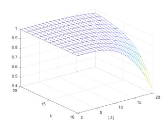
Figure 2: Plot of equation (7) for various values of $k$ and $|\mathcal{A}|$.

The lower bound on the probability given in Proposition 4 is a lower bound on the probability that pseudo-signal variables appear unaccompanied by other pseudo-signal variables in at least 2/3 regressions in which they appear. This bound is plotted in Figure 2. When $|\mathcal{A}|$ is of moderate size relative to $p=k^{3}$, the probability is close to one. The purpose of pairing highly correlated variables, as described in Section 1, is to make the set $\mathcal{A}$ as small as possible and thus increase probability (7), as variables that are highly correlated in sample with signal variables are then represented by a single one.

The result in Proposition 4 is conservative in that it focuses on the case where each pseudo-signal variable is the most significant in at least 2/3 regressions in which it appears. Cox reduction retains a variable if it is among the two most significant.

The first reduction retains all pseudo-signal variables whose marginal correlation with the response is sufficiently large and so mimics a conservative version of marginal screening that retains covariates with the largest $\hat{s}$ marginal correlations with the response, for $\hat{s}$ large. The two procedures differ in the set of retained pseudo-noise variables. The second round of Cox reduction, at which point the two procedures diverge more substantially, considers the joint explanatory power of sets of pseudo-signal variables.

6.3 Second reduction

Suppose that the index $e$, retained through the first reduction, is randomly arranged in a $k\times k$ square, where the dimension $k$ may be different from that of the first reduction. Let $\mathit{K}_{1}$ and $\mathit{K}_{2}$ be the variables that share a row or column with $e$ in the square and redefine $\mathcal{E}_{e:\mathit{K}}$ to be the event that the entry of $T_{Y:\mathit{K}}$ corresponding to $e\in\mathit{K}$ is significant at level $\alpha$. Then, the second round of Cox reduction retains the variable indexed by $e$ on the event $\mathcal{E}_{e:\mathit{K}_{1}}\cup\mathcal{E}_{e:\mathit{K}_{2}}$.

In contrast to the first round, pseudo-signal variables appear together in second-round regressions. Proposition 5 derives the expected number of pseudo-signal variables that share a row or column with a given $a\in\mathcal{A}$ in terms of the dimension of the square $k$ and the size of the set $\mathcal{A}$. For comparison, the analogous calculation for the cube is also provided. Figure 3 shows that this expectation is substantially larger in the second round.

Proposition 5.

Suppose the indices in $\mathcal{A}$ are randomised to positions in a $k\times k$ square. For a given index $a\in\mathcal{A}$, the expected number of indices from $\mathcal{A}_{-a}$ sharing a row or column with $a$ is

$$\frac{2(|\mathcal{A}|-1)}{k+1}.$$ (8)

In contrast, if the indices are randomised to positions of a $k\times k\times k$ cube, the expected number of indices from $\mathcal{A}_{-a}$ sharing a row, column or tube fibre with $a$ is

$$\frac{3(|\mathcal{A}|-1)}{k^{2}+k+1}.$$ (9)

(a) Round 1: $k\times k\times k$ cube

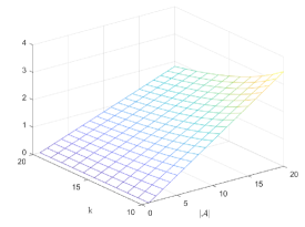
(b) Round 2: $k\times k$ square

Figure 3: Expected number of indices from $\mathcal{A}_{-a}$ sharing a fibre with $a$ for various values of $k$ and $|\mathcal{A}|$.

Combining Propositions 2 and 5, pseudo-signal variables are retained through the second reduction based on the significance of statistics of approximate form

$$\sigma^{-1}\|Y\|_{2}R(Y,(I-P_{\mathit{A}_{-a}})x_{a})$$

where $\mathit{A}\subseteq\mathcal{A}$ denotes the pseudo-signal variables appearing in a given row or column and $a\in\mathit{A}$. Since the second reduction compares the magnitude of these statistics to a pre-defined threshold, the retention of pseudo-signal variables is approximately independent of all pseudo-noise variables. Provided the dependence between pseudo-signal variables does not make $R(Y,(I-P_{\mathit{A}_{-a}})x_{a})$ small for many possible sets $\mathit{A}$ and indices $a$, Cox reduction will retain pseudo-signal variables.

The second reduction requires any apparent explanatory power to persist when the variable in question is accompanied by relatively strong companion variables. Its intended purpose was to differentiate variables in $\mathcal{S}$ from those in $\mathcal{S}^{c}\cap\mathcal{A}$, when $\mathcal{S}\subseteq\mathcal{A}$. Consider a regression of $Y$ on $X_{\mathit{A}}$ where $\mathit{A}\subseteq\mathcal{A}$ contains signal and noise indices. Lemma 3 shows that the entry of $\sigma T_{Y:A}$ corresponding to $a\in\mathit{A}$ is given by

$$\Delta_{1}+\Delta_{2}$$ (10)

where

$$\Delta_{1} = \sqrt{1-R^{2}(x_{a},X_{\mathit{A}_{-a}})}\theta^{0}_{a}\|x_{a}\|_{2}$$

$$\Delta_{2} = \|Y-X_{\mathit{A}}\theta^{0}_{\mathit{A}}\|_{2}R(Y-X_{\mathit{A}}\theta^{0}_{\mathit{A}},(I-P_{\mathit{A}_{-a}})x_{a}).$$

The term $\Delta_{1}$ describes the amount of the true signal corresponding to each variable that is recovered, and is equal to zero when $a$ indexes a noise variable. The term $\Delta_{2}$ characterises how well the variables in $A$ are able to recover the omitted signal $Y-X_{\mathit{A}}\theta^{0}_{\mathit{A}}$ and is bounded in magnitude by $\|Y-X_{\mathit{A}}\theta^{0}_{\mathit{A}}\|_{2}$. A regression of $Y$ on $X_{\mathit{A}}$ is able to distinguish between the noise and signal variables in $\mathit{A}$ if the term $\min_{a\in\mathcal{S}\cap\mathit{A}}|\Delta_{1}|$ is large in comparison to $\max_{a\in\mathit{A}}|\Delta_{2}|$. If $a$ indexes a noise variable, then $\Delta_{1}=0$ and $|\Delta_{2}|$ is minimised (up to terms involving $\epsilon$) when $\mathit{A}$ includes the signal variables that are not orthogonal to $x_{a}$. In contrast, $\Delta_{1}$ is largest for $a\in\mathcal{S}\cap\mathit{A}$ when colinearity between signal variables and other variables in $\mathit{A}$ is absent. Whether or not Cox reduction accurately differentiates variables in $\mathcal{S}$ from those in $\mathcal{S}^{c}\cap\mathcal{A}$ when $\mathcal{S}\subseteq\mathcal{A}$ therefore depends on the balance of colinearity among the variables present, and the proportion of signal that they encapsulate.

Pseudo-noise variables are retained through the second reduction based on the significance of statistics of approximate form

$$\sigma^{-1}\|(I-P_{\mathit{A}})Y\|_{2}R\{(I-P_{\mathit{A}})Y,(I-P_{\mathit{B}_{-b}})x_{b}\}$$

where $\mathit{B}\subset\mathcal{B}$ denotes the pseudo-noise variables appearing in the same regression as $\mathit{A}$; see Proposition 2 and equation (6). These statistics depend on the magnitude $\|(I-P_{\mathit{A}})Y\|_{2}$ and the correlation $R\{(I-P_{\mathit{A}})Y,(I-P_{\mathit{B}_{-b}})x_{b}\}$. When $\mathcal{B}$ contains only variables that are uncorrelated in population with the response and signal variables, $R((I-P_{\mathit{A}})Y,(I-P_{\mathit{B}_{-b}})x_{b})$ is a sample estimate of a null correlation coefficient, which is generally small for large enough sample sizes. Further, since the $t$-statistics are bounded by $\|(I-P_{\mathit{A}})Y\|_{2}$, pseudo-noise variables appearing alongside pseudo-signal variables are less likely to be retained by Cox reduction than pseudo-noise variables whose regression companions are of the same type.

In practice, the threshold $\alpha$ is chosen so that the set of retained variables is relatively stable across repeated rerandomisation of the indices in the two hypercubes. In view of the observations above, the set of pseudo-noise variables retained due to high spurious correlation $R((I-P_{\mathit{A}})Y,(I-P_{\mathit{B}_{-b}})x_{b})$ are expected to differ upon repeated rerandomisation of the variable indices in the hypercubes. In contrast, provided the dependence between pseudo-signal variables does not cause $R(Y,(I-P_{\mathit{A}_{-a}})x_{a})$ to be uniformly small over many sets $\mathit{A}$ and indices $a\in\mathit{A}$, pseudo-signal variables will be retained by Cox reduction irrespective of the arrangement of variable indices. Thus, a relatively stable set of retained variables over repeated rerandomisation suggests presence of variables with genuine explanatory power. If no threshold $\alpha$ results in a stable set of manageable size, this is a warning against the procedure for the data at hand.

6.4 Problematic situations

Section 5 discusses how the apparent effect of a signal variable can be diminished, producing a weak sample correlation with the outcome. Such a variable is relatively unlikely to be retained by Cox reduction.

In the second round, variables from $\mathcal{A}$ appear together with frequency depending on the dimension of the square. When a signal variable has a weak partial correlation with the response given many different variables from $\mathcal{A}$, it may be declared unimportant in both of its second-round regressions and hence discarded by Cox reduction.

While rerandomisation or a more systematic arrangement of the variable indices in the second reduction mitigates the latter situation, the former seems inescapable. Most variable selection procedures exclude the possibility that signal variables have weak marginal or partial correlations with the response. See Condition 3 in [21], and the definition of partial faithfulness or Assumption 4 in [4].

Another unfavourable situation, more problematic for marginal screening than for Cox reduction, is when a noise variable that is uncorrelated with all signal variables has a large sample correlation with the response purely by chance. Simulations in [21] pointed to large spurious correlations for large $p$. This was formalised in [22] which established the limiting distribution of the maximum spurious correlation. The distributions of other order statistics were not discussed. Any spurious noise variable would be contained in $\mathcal{A}$ and likely survive the first reduction. Depending on the random arrangement of variables in the square, it may also survive the second reduction. Similarly, noise variables may be retained when multiple correlation coefficients between uncorrelated variables are spuriously large.

In view of the model assessment phase, inclusion of noise variables is less problematic than omission of signal variables provided there are not so many as to make assessment of models practically infeasible. Sample splitting and rerandomisation, discussed in Section 7, reduce the survival probability of noise variables.

7 Recommended improvements to Cox reduction

7.1 Alternating subsamples

We propose using a different portion of the sample for each reduction round, breaking the dependence between analyses in the first and second reduction and thereby reducing the probability that irrelevant noise variables appear correlated with the response in both rounds. Let $\mathcal{I}$ be a subset of $\{1,\dots,n\}$. The split-sample version of Cox reduction uses observations indexed by $\mathcal{I}$ for the first reduction and the model assessment phase, and those indexed by $\mathcal{I}^{c}$ for the second reduction. For more than two reduction rounds, alternation should continue in this way. We recommend including $30-40\%$ of observations in $\mathcal{I}$ for the two-stage procedure, based on the relative difficulty of the stages.

7.2 Rerandomisation

A benefit of Cox reduction is the external source of randomness from the arrangement of variable indices in successive hypercubes. This provides a way of internally calibrating the procedure by rerandomising the variable indices. Battey and Cox [1] suggested this as a check on the stability of $\hat{\mathcal{S}}$. An elaboration is to rerandomise repeatedly, resulting in sets $\hat{\mathcal{S}}_{1},\hat{\mathcal{S}}_{2},\ldots$, and only retain variables in the final set $\hat{\mathcal{S}}$ if they are present most of the time, e.g. in at least half the rerandomisation outcomes. With this adaptation, Cox reduction is less dependent on the particular set of variables appearing in regressions together, reducing the chances that signal variables are omitted due to small partial correlations or that noise variables are retained due to high spurious correlation.

A natural and partially refutable criticism is that the procedure entails at least one tuning parameter (from the second-round reduction), increased to two when rerandomisation is introduced. In practice, selection of tuning parameters is guided by stability of the set $\hat{\mathcal{S}}$ and is rarely problematic. If there appears to be no choice of tuning pair that delivers a stable outcome, that is a warning against the procedure. The ability of Cox reduction to reveal its own fragility on the data at hand is an advantage over the alternatives discussed in Section 5.

8 Numerical performance

Section 2 of the supplementary material shows the numerical performance of Cox reduction and the proposed construction of the model confidence set. Simulated data was generated to compare marginal screening and LASSO penalised regression to Cox reduction in the setting laid out in Section 6. Cox reduction and marginal screening both performed well, retaining all signal variables in the comprehensive model and yielding a model confidence set with high simulated coverage probability. In contrast, the undertuned LASSO failed to include all signal variables in the comprehensive model when correlations among variables were high and signal strengths were low. The size of the model confidence set constructed from marginal screening contained more models on average than that obtained from Cox reduction, as expected based on the discussion in Section 5.

Cox reduction was also applied to real covariate data with randomly generated artificial responses, so as to explore its performance in the presence of more complicated dependence structures. Three cases exemplify how Cox reduction can perform better or worse than marginal screening. In the first example, both procedures fail to identify signal variables that are weakly correlated with the response variable. When multiple noise variables are correlated with a signal, it is possible that these noise variables appear marginally stronger than the signal variables. In these settings, Cox reduction is able to detect the signal variables while marginal screening cannot, as illustrated in the second example. The final example shows that when signal variables are weakly correlated with each other, marginal screening may outperform Cox reduction.

9 Further discussion

9.1 Rebuttal of an alternative approach

A natural attempt to construct confidence sets of models uses the LASSO or similar on $B$ bootstrap samples, obtained by sampling $n$ observations with replacement. This suggestion can be refuted in the light of [35, 34].

Let the true positive rate be the proportion of signal variables selected by the LASSO and the false discovery rate be the proportion of selected variables that are noise variables. Su et al. [35] show that even under idealised conditions with large signal strengths and uncorrelated variables, the false discovery rate is lower bounded by a function of the true positive rate with probability one. Further, [34] shows that the first noise variable is selected earlier on the LASSO path than the final signal variable. Hence, each model either includes the full set of signal variables contaminated by noise variables, or does not include the full set of signal variables. These conclusions hold with probability tending to one in the notional double asymptotic regime in which $p$ grows with $n$. As a result, with probability close to one, the true model is never selected and a model confidence set constructed in this way has coverage probability close to zero.

9.2 Cox reduction with unknown variance

An unknown error variance $\sigma$ can either be estimated prior to Cox reduction based on all $p$ covariates or estimated anew in each of the regressions that are run. The former approach results in an unbiased estimate, whilst the latter typically produces biased estimates from regressions omitting signal variables. Nevertheless, the latter is preferable as a severely biased estimate indicates that the joint explanatory power of covariates appearing in a regression together is weak, making it less likely that these covariates are retained through the second round of Cox reduction. The associated Wald statistic is

$$T_{Y:K}=\hat{\sigma}_{\mathit{K}}^{-1}D_{\mathit{K}}^{-1/2}\hat{\theta}_{Y:\mathit{K}},\quad\quad\quad\hat{\sigma}^{2}_{\mathit{K}}=\frac{\|Y-X_{\mathit{K}}\hat{\theta}_{Y:\mathit{K}}\|_{2}^{2}}{n-|\mathit{K}|}$$

where $D_{\mathit{K}}$ is a diagonal matrix with entries given by the diagonal entries of $(X_{\mathit{K}}^{T}X_{\mathit{K}})^{-1}$. This choice does not affect the first-round reduction, which is based on the relative significance of variables in a given regression. Its effect in the second round is to de-emphasise covariates appearing in regressions with a weak signal.

If it is instead decided to estimate $\sigma$ prior to Cox reduction, suitable estimators are in [19], [33] and [16]. See [31] for a numerical comparison of their performance. As the relative significance of covariates are unaffected by estimation of $\sigma$, an equivalent approach sets $\sigma$ to be an arbitrary value, adjusting the second-round significance level to give a stable comprehensive model of manageable size.

9.3 Systematic arrangement of variables in the second round

Expression (10) shows that differentiation between Cox reduction and marginal screening can be achieved by forcing second-round regressions to contain correlated signal and noise variables from $\mathcal{A}$. This suggests a more systematic arrangement of variables in the square in which indices $\mathit{E}$ and $\mathit{F}$ for which $|R(x_{\mathit{E}},x_{\mathit{F}})|\gg 0$ appear together in rows or columns. In the description of Cox reduction outlined in Section 1 variables with high sample correlation were paired or grouped, and so the comprehensive model would either include both variables in a pair or neither. To distinguish between signal and noise variables that are highly correlated, it would be necessary to unpair the variables at the second reduction. Thus any second-round regression including a representative variable for a pair or larger group would include all members. Further analysis is needed to ascertain any optimal arrangement of variables in the second round to maximise the probability of retaining signal variables.

9.4 Binary responses

As discussed in Section 3, Scheffé [32] emphasised the approximate validity of inference based on a notional linear model, owing to the randomisation. In ongoing work not reported here [28], we formalise this intuition beyond the context of Cox reduction when the outcomes are generated from a linear logistic model. Generative binary models, when fitted by maximum likelihood, are problematic in the second stage of Cox reduction, where many combinations of strong variables form a separating hyperplane, that is, produce no classification errors within sample. Ordinary least squares fitting overcomes the difficulties.

9.5 Prediction

The argument for confidence sets of models is somewhat weakened when prediction is the primary goal. However, stability of the predictor over time and in different contexts is important and more likely with a model that has an underlying interpretation as well as immediate predictive success. By consideration of prediction intervals for each model in $\mathcal{M}$, we account both for model uncertainty and statistical uncertainty. Overlapping prediction intervals are reassuring, while those differing considerably point to instability of the predictor under alternative circumstances. See Section S3 of the supplementary material for an example.

Acknowledgements. The work was partially supported by a UK Engineering and Physical Sciences Research Fellowship (to H.S.B).

Availability of source code. Source code for implementing Cox reduction and constructing confidence sets of models is available from: www.ma.imperial.ac.uk/ hbattey/softwareCube.html. The more user-interfaced R package HCmodelSets is accompanied by a detailed guide to usage [26]. Source code implementing some of the refinements discussed in the present work, such as those used in the simulations in Section S2.1 of the supplementary material, is available from https://github.com/rm-lewis.

Appendix A Proofs of main results

Throughout this section, let $\mathit{E},\mathit{F}\subset\{1,\dots,p\}$ be such that $|\mathit{E}\cup\mathit{F}|<n$ with $E\cap F=\emptyset$. These sets will always be used to index columns of $X$. Define $\mathit{K}=\mathit{E}\cup\mathit{F}$ to be the indices appearing in a given traversal of the hypercube. In a regression of $Y$ on $X_{\mathit{K}}$, let

$$\hat{\theta}_{Y:\mathit{K}} = (X_{\mathit{K}}^{T}X_{\mathit{K}})^{-1}X_{\mathit{K}}^{T}Y,$$

and use $\hat{\theta}_{Y:\mathit{E}.\mathit{F}}$ and $\hat{\theta}_{Y:\mathit{F}.\mathit{E}}$ to denote the entries of $\hat{\theta}_{Y:\mathit{K}}$ corresponding to the sets $\mathit{E}$ and $\mathit{F}$ respectively. Let $\hat{\theta}_{F:E}=(X_{E}^{T}X_{E})^{-1}X_{E}^{T}X_{F}$. Similarly, let $T_{Y:\mathit{K}}$ be the Wald-type statistic obtained from a linear regression of $Y$ on $X_{\mathit{K}}$, and denote its components corresponding to $\mathit{E}$ and $\mathit{F}$ by $T_{Y:\mathit{E}.\mathit{F}}$ and $T_{Y:\mathit{F}.\mathit{E}}$ respectively. More precisely,

$$T_{Y:\mathit{K}}=\sigma^{-1}D_{\mathit{K}}^{-1/2}\hat{\theta}_{Y:\mathit{K}}$$

where $D_{\mathit{K}}$ is a diagonal matrix with entries given by the diagonal entries of $(X_{\mathit{K}}^{T}X_{\mathit{K}})^{-1}$. The notation

$$(X_{K}^{T}X_{K})^{-1}_{(\mathit{E},\mathit{E})}$$

will be used to denote the rows and columns of the matrix $(X_{\mathit{K}}^{T}X_{\mathit{K}})^{-1}$ corresponding to the set $\mathit{E}$.

Proof of Proposition 1..

The log-likelihood ratio test statistic can be expressed as

$$w(\mathcal{S}_{m})/2 = \sup_{\eta\in\text{Col-Sp}(\widetilde{X})}\bar{\ell}(\eta)-\sup_{\eta\in\text{Col-Sp}(\widetilde{X}_{m})}\bar{\ell}(\eta)$$

$$= \sup_{h_{1}\in\text{Col-Sp}(\widetilde{X})}\bar{\ell}(\eta^{0}+h_{1})-\sup_{h_{0}\in\{\text{Col-Sp}(\widetilde{X}_{m})-\eta^{0}\}}\bar{\ell}(\eta^{0}+h_{0})$$

as $\eta^{0}$ is assumed to be in the column span of $\widetilde{X}$ but not necessarily in the column span of $\widetilde{X}_{m}$. Let $\hat{h}_{0}=\hat{\eta}_{m}-\eta^{0}$ and $\hat{h}_{1}=\hat{\eta}-\eta^{0}$ be the maximisers. By assumption, $\|\hat{h}_{0}\|_{3}^{3},\,\|\hat{h}_{1}\|_{3}^{3}=O_{P}(n^{-1/2})$. Define $M_{n}$ to be a sequence converging to zero as $n\rightarrow\infty$ so that $\|\hat{h}_{1}\|_{3}/M_{n}=o_{P}(1)$ and $\|\hat{h}_{0}\|_{3}/M_{n}=o_{P}(1)$. For example, $M_{n}=n^{-1/7}$. Then, with probability converging to one, $\hat{h}_{1},\hat{h}_{0}\in B_{n}$, the $\ell_{3}$-ball of radius $M_{n}$ about zero, and so

$$w(\mathcal{S}_{m})/2 = \Delta_{1}-\Delta_{0}+o_{P}(1)$$

where

$$\Delta_{1} = \sup_{h_{1}\in H^{(1)}_{n}}\bar{\ell}(\eta^{0}+h_{1})-\bar{\ell}(\eta^{0})$$

$$\Delta_{0} = \sup_{h_{0}\in H^{(0)}_{n}}\bar{\ell}(\eta^{0}+h_{0})-\bar{\ell}(\eta^{0}),$$

$H^{(1)}_{n}=\text{Col-Sp}(\widetilde{X})\cap B_{n}$ and

$$H^{(0)}_{n}=(\text{Col-Sp}(\widetilde{X}_{m})-\eta^{0})\cap B_{n}.$$

Let $U^{0}=\nabla_{\eta}\bar{\ell}(\eta^{0})$ and $J^{0}=-\nabla_{\eta\eta}^{2}\bar{\ell}(\eta^{0})$. For $h_{1}\in H^{(1)}_{n}$, $\|h_{1}\|_{3}\leq M_{n}$ and $h_{1}=\widetilde{Q}\beta$ for some $\beta\in\mathbb{R}^{\hat{r}}$ and $\widetilde{Q}$ defined in the statement of the proposition. So, applying the local asymptotic expansion,

$$\Delta_{1} = \sup_{\beta:\,\widetilde{Q}\beta\in H^{(1)}_{n}}\{\beta^{T}\widetilde{Q}^{T}U^{0}-\frac{1}{2}\beta^{T}\widetilde{Q}^{T}J^{0}\widetilde{Q}\beta\}+o_{P}(1).$$

The supremum is achieved at

$$\beta=(\widetilde{Q}^{T}J^{0}\widetilde{Q})^{-1}\widetilde{Q}^{T}U^{0}$$

satisfying

$$||\widetilde{Q}\beta||_{3}^{3}\leq||\widetilde{Q}\beta||_{\infty}||\widetilde{Q}\beta||_{2}^{2}=O_{P}(n^{-1/2})=o_{P}(M_{n}^{3})$$

because, letting $Z=(\widetilde{Q}^{T}J^{0}\widetilde{Q})^{-1/2}\widetilde{Q}^{T}U^{0}$,

$$||\beta||_{2} = n^{-1/2}||(\widetilde{Q}^{T}J^{0}\widetilde{Q}/n)^{-1/2}Z||_{2}$$

$$\leq n^{-1/2}||(\widetilde{Q}^{T}J^{0}\widetilde{Q}/n)^{-1/2}||_{2}||Z||_{2}$$

$$= O_{P}(n^{-1/2})$$

by (c), (d) and $||\widetilde{Q}\beta||_{\infty}\leq\max_{i=1}^{n}||\widetilde{q}_{i}||_{2}||\beta||_{2}$. This maximiser lies in $B_{n}$ with probability converging to one and so

$$\Delta_{1} = \|(\widetilde{Q}^{T}J^{0}\widetilde{Q})^{-1/2}\widetilde{Q}^{T}U^{0}\|^{2}_{2}/2+o_{P}(1).$$

For $h_{0}\in H^{(0)}_{n}$, $\|h_{0}\|_{3}\leq M_{n}$ and $h_{0}=\widetilde{Q}_{m}\alpha+v$ where $v=-(I-P_{m})\eta^{0}$ and $\alpha\in\mathbb{R}^{r_{m}}$. So,

$$\Delta_{0} = \sup_{\alpha:\,(\widetilde{Q}_{m}\alpha+v)\in H^{(0)}_{n}}\{(\widetilde{Q}_{m}\alpha+v)^{T}U^{0}-\frac{1}{2}(\widetilde{Q}_{m}\alpha+v)^{T}J^{0}(\widetilde{Q}_{m}\alpha+v)\}+o_{P}(1).$$

By assumption $\|v\|_{2}=o(n^{-1/2})$ and

$$n^{-1/2}\|\widetilde{Q}_{m}\alpha\|_{2}\leq n^{-1/2}\|h_{0}\|_{2}\leq n^{-1/3}\|h_{0}\|_{3}=o(1).$$

So,

$$|v^{T}U^{0}| \leq \sqrt{n}\|v\|_{2}\|n^{-1/2}U_{0}\|_{2}=o_{P}(1)$$

$$|v^{T}J^{0}\widetilde{Q}_{m}\alpha| = \|\sqrt{n}v\|_{2}\|n^{-1/2}\widetilde{Q}_{m}\alpha\|_{2}\|J_{0}\|_{2}=o_{P}(1)$$

$$|v^{T}J^{0}v| \leq \|n^{-1}J^{0}\|_{2}\|\sqrt{n}v\|^{2}_{2}=o_{P}(1).$$

Thus,

$$\Delta_{0} = \sup_{\alpha:\,(\widetilde{Q}_{m}\alpha+v)\in H^{(0)}_{n}}\{(\widetilde{Q}_{m}\alpha)^{T}U^{0}-\frac{1}{2}(\widetilde{Q}_{m}\alpha)^{T}J^{0}(\widetilde{Q}_{m}\alpha)\}+o_{P}(1)$$

and maximising this expression gives

$$\Delta_{0} = \|(\widetilde{Q}_{m}^{T}J^{0}\widetilde{Q}_{m})^{-1/2}\widetilde{Q}_{m}^{T}U^{0}\|^{2}_{2}/2+o_{P}(1).$$

Combining equations (A) and (A)

$$w(\mathcal{S}_{m}) = \|(\widetilde{Q}^{T}J^{0}\widetilde{Q})^{-1/2}\widetilde{Q}^{T}U^{0}\|^{2}_{2}-\|(\widetilde{Q}_{m}^{T}J^{0}\widetilde{Q}_{m})^{-1/2}\widetilde{Q}_{m}^{T}U^{0}\|^{2}_{2}+o_{P}(1)$$

$$= (\Sigma^{-1/2}Z)^{T}\Gamma\Sigma^{-1/2}Z+o_{P}(1)$$

where $Z=n^{-1/2}\widetilde{Q}^{T}U^{0}$, $n\Sigma=\widetilde{Q}^{T}J^{0}\widetilde{Q}$, $n\Sigma_{mm}=\widetilde{Q}_{m}^{T}J^{0}\widetilde{Q}_{m}$ and

$$\Gamma=\mathbbm{I}-\Sigma^{1/2}\begin{pmatrix}\Sigma_{mm}^{-1}&0\\ 0&0\end{pmatrix}\Sigma^{1/2}.$$

The matrix $\Gamma$ is positive semi-definite of rank $\hat{r}-r_{m}$ with eigenvalues equal to one or zero. This is because

$$\lambda\left\{\Sigma^{1/2}\begin{pmatrix}\Sigma_{mm}^{-1}&0\\ 0&0\end{pmatrix}\Sigma^{1/2}\right\} = \lambda\left\{\begin{pmatrix}\Sigma_{mm}^{-1}&0\\ 0&0\end{pmatrix}\Sigma\right\}$$

where for any square matrix $M$, $\lambda(M)$ is the set of eigenvalues of $M$. As $\Sigma_{mm}$ are the entries of $\Sigma$ in the first $r_{m}$ rows and $r_{m}$ columns, this set consists of the eigenvalues of an upper triangular matrix with $r_{m}$ ones and $\hat{r}-r_{m}$ zeroes on the diagonal. Thus, the set of eigenvalues of $\Gamma$ consists of $r_{m}$ zeroes and $\hat{r}-r_{m}$ ones. Write $\Gamma=P^{T}\Lambda P$ where $P$ is an orthonormal matrix and $\Lambda$ is a diagonal matrix with $\hat{r}-r_{m}$ ones and $r_{m}$ zeroes on the diagonal. Then,

$$w(\mathcal{S}_{m}) = (P\Sigma^{-1/2}Z)^{T}\Lambda(P\Sigma^{-1/2}Z)+o_{P}(1)$$

$$= \sum_{i=1}^{\hat{r}-r_{m}}(P\Sigma^{-1/2}Z)^{2}_{i}+o_{P}(1)$$

and by assumption, $P\Sigma^{-1/2}Z\overset{d}{\longrightarrow}N(0,\mathbb{I})$. As asymptotically $w(\mathcal{S}_{m})$ is the sum of the squares of $\hat{r}-r_{m}$ independent standard normal random variables

$$w(\mathcal{S}_{m})\overset{d}{\longrightarrow}\chi^{2}_{\hat{r}-r_{m}}$$

and so the result follows. ∎

Lemma 1.

$$\hat{\theta}_{Y:\mathit{E}}=\hat{\theta}_{Y:\mathit{E}.\mathit{F}}+(\hat{\theta}_{\mathit{F}:\mathit{E}})^{T}\hat{\theta}_{Y:\mathit{F}.\mathit{E}}.$$

Proof.

Let $\mathit{K}=\mathit{E}\cup\mathit{F}$. By definition,

$$\hat{\theta}_{Y:\mathit{E}} = (X_{\mathit{E}}^{T}X_{\mathit{E}})^{-1}X_{\mathit{E}}^{T}P_{\mathit{K}}Y+(X_{\mathit{E}}^{T}X_{\mathit{E}})^{-1}X_{\mathit{E}}^{T}(I-P_{\mathit{K}})Y$$

$$= (X_{\mathit{E}}^{T}X_{\mathit{E}})^{-1}X_{\mathit{E}}^{T}P_{\mathit{K}}Y$$

$$= (X_{\mathit{E}}^{T}X_{\mathit{E}})^{-1}X_{\mathit{E}}^{T}X_{\mathit{K}}\hat{\theta}_{Y:\mathit{K}}$$

$$= (I,(X_{\mathit{E}}^{T}X_{\mathit{E}})^{-1}X_{\mathit{E}}^{T}X_{\mathit{F}})\hat{\theta}_{Y:\mathit{K}}$$

$$= \hat{\theta}_{Y:\mathit{E}.\mathit{F}}+(\hat{\theta}_{\mathit{F}:\mathit{E}})^{T}\hat{\theta}_{Y:\mathit{F}.\mathit{E}}$$

where we have assumed without loss of generality that $\mathit{E}$ indexes the first few columns of $X_{K}$. Further,

$$\hat{\theta}_{Y:\mathit{E}}=\hat{\theta}_{Y:\mathit{E}.\mathit{F}}\iff(\hat{\theta}_{\mathit{F}:\mathit{E}})^{T}\hat{\theta}_{Y:\mathit{F}.\mathit{E}}=0.$$

∎

Lemma 2.

Suppose $|\mathit{E}|=1$. Then,

$$T_{Y:\mathit{E}.\mathit{F}}=\sigma^{-1}\|Y\|_{2}R(Y,(I-P_{\mathit{F}})x_{\mathit{E}}).$$

Proof.

By Lemma 4 and the definitions of marginal and multiple sample correlation coefficients,

$$\hat{\theta}_{Y:\mathit{E}.\mathit{F}} = \{x_{\mathit{E}}^{T}(I-P_{\mathit{F}})x_{\mathit{E}}\}^{-1}x_{\mathit{E}}^{T}(I-P_{\mathit{F}})Y$$

$$= \frac{R(Y,(I-P_{\mathit{F}})x_{\mathit{E}})\|Y\|_{2}}{\|x_{\mathit{E}}\|\sqrt{1-R^{2}(x_{\mathit{E}},X_{\mathit{F}})}}.$$

By writing the inverse of a matrix in terms of a Schur complement,

$$(X_{\mathit{K}}^{T}X_{\mathit{K}})^{-1}_{(\mathit{E},\mathit{E})} = (x_{\mathit{E}}^{T}(I-P_{\mathit{F}})x_{\mathit{E}})^{-1}$$

$$= \|x_{\mathit{E}}\|_{2}^{-2}(1-R^{2}(x_{\mathit{E}},X_{\mathit{F}}))^{-1}.$$

Combining these equations gives the desired result. ∎

Proof of Proposition 2.

The result follows directly from Lemmas 7 and 8 in Appendix B. ∎

Proof of Proposition 3.

Let $\epsilon=M\log(|\mathcal{B}|)$ with $M>0$. By a union bound,

$$\mathbb{P} \left\{n\Delta(1)>\epsilon\right\}\leq\mathbb{P}\left\{\max_{\mathit{B}\subset\mathcal{B},|\mathit{B}|=k}nR^{2}(Y,X_{\mathit{B}})>\epsilon\right\}$$

$$+\mathbb{P}\left\{\max_{\mathit{B}\subset\mathcal{B},|\mathit{B}|=k-1}nR^{2}(Y,X_{\mathit{B}})>\epsilon\right\}$$

$$+|\mathcal{A}|\max_{\mathit{A}\subseteq\mathcal{A},|\mathit{A}|=1}\mathbb{P}\left\{\max_{\mathit{B}\subset\mathcal{B},|\mathit{B}|=k-1}nR^{2}(X_{\mathit{A}},X_{\mathit{B}})>\epsilon\right\}$$

and so it is sufficient to consider the limiting distribution of the maximum spurious correlation between a vector and an independent random matrix consisting of $k$ or $k-1$ columns. We focus on the term $R^{2}(X_{\mathit{A}},X_{\mathit{B}})$ although the results follow identically for $R^{2}(Y,X_{\mathit{B}})$. Under the assumptions in the proposition, Theorem 3.1 in [22] states that there exists a constant $C>0$ independent of $|\mathcal{B}|$, $k$ and $n$ such that

$$\sup_{\epsilon\geq 0}|\mathbb{P}\{n\max_{\mathit{B}\subset\mathcal{B},\,|\mathit{B}|=k-1}R^{2}(X_{\mathit{A}},X_{\mathit{B}})>\epsilon\}-\mathbb{P}\{\widetilde{R}^{2}>\epsilon\}|\leq Cn^{-1/8}[\max\{\log(|\mathcal{B}|),\log n\}]^{7/8}$$

where

$$\widetilde{R}^{2}=Z_{(|\mathcal{B}|)}^{2}+\dots+Z_{(|\mathcal{B}|-k+2)}^{2}$$

with $Z\sim N_{|\mathcal{B}|}(0,I)$ and

$$Z_{(1)}^{2}\leq Z_{(2)}^{2}\leq\dots\leq Z_{(|\mathcal{B}|)}^{2}$$

are the order statistics of $\{Z_{j}^{2}\}_{j=1}^{|\mathcal{B}|}$. The aim is to obtain the rate at which $\mathbb{P}\{\widetilde{R}^{2}>\epsilon\}$ converges to zero. Let $M_{n}=\max_{i=1,\dots|\mathcal{B}|}Z_{i}$ and $L_{n}=\max_{i=1,\dots|\mathcal{B}|}\{-Z_{i}\}$. As a maximum of i.i.d. standard Gaussian random variables, [24] shows that $a_{n}^{-1}(M_{n}-b_{n})$ converges in distribution to a Gumbel distribution where $a_{n}=b_{n}^{-1}$ and

$$b_{n} = \sqrt{2\log(|\mathcal{B}|)}-\frac{\log{\log(|\mathcal{B}|)}+\log(4\pi)}{2\sqrt{2\log(|\mathcal{B}|)}}+O\{(\log|\mathcal{B}|)^{-1}\}.$$

A similar result holds for $L_{n}$. The rate of convergence to a Gumbel distribution is $\{\log(|\mathcal{B}|)\}^{-1}$, and so

$$\mathbb{P}(\widetilde{R}^{2}>\epsilon) \leq \mathbb{P}\{(k-1)Z^{2}_{(|\mathcal{B}|)}>\epsilon\}$$ (11)

$$\leq \mathbb{P}\{(k-1)^{1/2}M_{n}>\sqrt{\epsilon}\}+\mathbb{P}\{(k-1)^{1/2}L_{n}>\sqrt{\epsilon}\}$$

$$\leq 2\left\{1-\exp\left(-e^{-f_{n}}\right)+\eta_{n}\right\}$$

where, for $\epsilon=M\log(|\mathcal{B}|)$ with $M>0$ large enough,

$$\max\{f_{n}^{-1},\,\eta_{n}\} = O[\{\log(|\mathcal{B}|)\}^{-1}].$$

As $e^{x}\geq 1+x$ for all $x$, we have

$$1-\exp\left(-e^{-f_{n}}\right) \leq 1-\exp\left\{\frac{-1}{f_{n}+1}\right\}\leq(1+f_{n})^{-1},$$

and so

$$\mathbb{P}\left\{n\max_{\begin{subarray}{c}\mathit{B}\subset\mathcal{B},\\ |\mathit{B}|=k-1\end{subarray}}R^{2}(X_{\mathit{A}},X_{\mathit{B}})>\epsilon\right\}=O\left(\max\left\{\epsilon_{n},\log(|\mathcal{B}|)^{-1}\right\}\right)$$

where $\epsilon_{n}=n^{-1/8}\max\{\log(|\mathcal{B}|),\log n\}^{7/8}$. Using similar arguments,

$$\mathbb{P}(n\Delta(1)>\epsilon)=O\left(|\mathcal{A}|\max\left\{\epsilon_{n},\log(|\mathcal{B}|)^{-1}\right\}\right).$$

When $|\mathcal{A}|=o\{\log(|\mathcal{B}|)\}$ and $|\mathcal{A}|^{8/7}\log\{|\mathcal{B}|n\}=o(n^{1/7})$, all terms on the right hand side converge to zero and so

$$\Delta(1)=O_{P}(\log(|\mathcal{B}|)/n).$$

The result follows when $\log(|\mathcal{B}|)/n=o(1)$. ∎

Proof of Proposition 4.

We can condition on the event $\mathcal{G}$ that each variable in $\mathcal{A}$ appears unaccompanied by other pseudo-signal variables in at least 2/3 regressions in which it appears. A lower bound on the probability that this event occurs is given in Lemma 9. On the event $\mathcal{G}$, every pseudo-signal variable will survive the first round of reduction if

$$\min_{A\subseteq\mathcal{A},\,|A|=1}\min_{\mathit{B}\in\mathcal{B}_{k}}\{|T_{Y:\mathit{A}.\mathit{B}}|-\|T_{Y:\mathit{B}.\mathit{A}}\|_{\infty}\}>0$$ (12)

where $\mathcal{B}_{k}=\{\mathit{B}\subseteq\mathcal{B}:|\mathit{B}|=k-1\}$. By Proposition 2, Lemma 2 and Lemma 8,

$$T_{Y:\mathit{A}.\mathit{B}} = \sigma^{-1}\|Y\|_{2}R(Y,x_{\mathit{A}})+\delta_{A.B}$$

$$T_{Y:\mathit{B}.\mathit{A}} = \delta_{B.A}^{(1)}+\delta_{B.A}^{(2)}$$

where provided $R(X_{\mathit{A}},X_{\mathit{B}})<1-c$, there exists $C>0$ depending only on $c$ such that,

$$|\delta_{A.B}| \leq C\sigma^{-1}\|Y\|_{2}\{R(X_{\mathit{A}},X_{\mathit{B}})+R(Y,X_{\mathit{B}})\}$$

$$\|\delta^{(1)}_{B.A}\|_{\infty} \leq \sigma^{-1}\|Y\|_{2}\{R(X_{\mathit{A}},X_{\mathit{B}})+R(Y,X_{\mathit{B}})\}$$

$$\|\delta_{B.A}^{(2)}\|_{\infty} \leq C\sigma^{-1}\|\widetilde{Y}\|_{2}R(X_{\mathit{A}},X_{\mathit{B}}).$$

Thus, (12) occurs if for all $\mathit{A}\subseteq\mathcal{A}$ with $|A|=1$, $\mathit{B}\in\mathcal{B}_{k}$,

$$\sigma^{-1}\|Y\|_{2}|R(Y,x_{\mathit{A}})|-|\delta_{\mathit{A}.\mathit{B}}|>\|\delta_{B.A}^{(1)}\|_{\infty}+\|\delta_{B.A}^{(2)}\|_{\infty}$$

By assumption, there exists $\epsilon>0$ such that for $n$ large enough,

$$\min_{\mathit{A}\subset\mathcal{A},\,|A|=1}|R(Y,x_{\mathit{A}})|>\sigma\epsilon$$

and

$$\max_{\mathit{A}\subset\mathcal{A},\,|A|=1,\mathit{B}\in\mathcal{B}_{k}}\max\{|\delta_{A.B}|,\|\delta_{B.A}^{(1)}\|_{\infty},\|\delta_{B.A}^{(2)}\|_{\infty}\}\leq\epsilon\|Y\|_{2}/4.$$

Then, condition (A) holds and the result follows. ∎

Proof of Proposition 5.

First consider the $k\times k$ square. Let $\mathcal{G}_{a,a_{0}}$ be the event that indices $a$ and $a_{0}$ share a row or column. The expected number of indices from $\mathcal{A}_{-a}$ sharing a row or column fibre with $a$ is given by

$$\mathbb{E}\left[\sum_{a_{0}\in\mathcal{A}_{-a}}\mathbbm{1}\{\mathcal{G}_{a,a_{0}}\}\right]=\frac{2(|\mathcal{A}|-1)(k-1)}{(k^{2}-1)}$$

as conditional on the location of $a$ in the square, there are $2(k-1)$ out of a total of $k^{2}-1$ locations for $a_{0}$ that ensure that $a$ and $a_{0}$ share a row or column.

The arguments for the $k\times k\times k$ cube are similar. Now let $\mathcal{G}_{a,a_{0}}$ be the event that indices $a$ and $a_{0}$ share a row, column or tube fibre. The expected number of indices from $\mathcal{A}_{-a}$ sharing a row, column or tube fibre with $a$ is given by

$$\mathbb{E}\left[\sum_{a_{0}\in\mathcal{A}_{-a}}\mathbbm{1}\{\mathcal{G}_{a,a_{0}}\}\right] = \frac{3(|\mathcal{A}|-1)(k-1)}{(k^{3}-1)}$$

as conditional on the location of $a$ in the cube, there are $3(k-1)/(k^{3}-1)$ locations for $a_{0}$ to ensure that $a$ and $a_{0}$ share a row, column or tube fibre. ∎

Lemma 3.

Suppose $|\mathit{E}|=1$. Then

$$\sigma T_{Y:\mathit{E}.\mathit{F}}=\Delta_{1}+\Delta_{2}$$

where

$$\Delta_{1} = \sqrt{1-R^{2}(x_{\mathit{E}},X_{\mathit{F}})}\theta^{0}_{\mathit{E}}\|x_{\mathit{E}}\|_{2}$$

$$\Delta_{2} = \|Y-X_{\mathit{K}}\theta^{0}_{\mathit{K}}\|_{2}R(Y-X_{\mathit{K}}\theta^{0}_{\mathit{K}},(I-P_{\mathit{F}})x_{\mathit{E}})$$

where $\mathit{K}=\mathit{E}\cup\mathit{F}$.

Proof.

By definition,

$$(X_{\mathit{K}}^{T}X_{\mathit{K}})^{-1}X_{\mathit{K}}^{T}Y = \theta^{0}_{\mathit{K}}+(X_{\mathit{K}}^{T}X_{\mathit{K}})^{-1}X_{\mathit{K}}^{T}(Y-X_{\mathit{K}}\theta^{0}_{\mathit{K}}).$$

Further,

$$(X_{\mathit{K}}^{T}X_{\mathit{K}})^{-1}_{(\mathit{E},\mathit{E})} = \|x_{\mathit{E}}\|_{2}^{-2}(1-R^{2}(x_{\mathit{E}},X_{\mathit{F}}))^{-1},$$

so

$$\sigma T_{Y:\mathit{E}.\mathit{F}} = \sqrt{1-R^{2}(x_{\mathit{E}},X_{\mathit{F}})}\theta^{0}_{\mathit{E}}\|x_{\mathit{E}}\|_{2}+\sigma T_{(Y-X_{\mathit{K}}\theta^{0}_{\mathit{K}}):\mathit{E}.\mathit{F}}.$$

The result follows by applying Lemma 2 to the second term. ∎

Appendix B Proofs of additional results

The notation in this section follows the notation in Appendix A.

Lemma 4.

$$\hat{\theta}_{Y:\mathit{E}.\mathit{F}} = \{X_{\mathit{E}}^{T}(I-P_{\mathit{F}})X_{\mathit{E}}\}^{-1}X_{\mathit{E}}^{T}(I-P_{\mathit{F}})Y$$

$$\hat{\theta}_{Y:\mathit{F}.\mathit{E}} = \{X_{\mathit{F}}^{T}(I-P_{\mathit{E}})X_{\mathit{F}}\}^{-1}X_{\mathit{F}}^{T}(I-P_{\mathit{E}})Y.$$

Proof.

By definition

$$\begin{pmatrix}X_{\mathit{E}}^{T}X_{\mathit{E}}&X_{\mathit{E}}^{T}X_{\mathit{F}}\\ X_{\mathit{F}}^{T}X_{\mathit{E}}&X_{\mathit{F}}^{T}X_{\mathit{F}}\end{pmatrix}\begin{pmatrix}\hat{\theta}_{Y:\mathit{E}.\mathit{F}}\\ \hat{\theta}_{Y:\mathit{F}.\mathit{E}}\end{pmatrix}=\begin{pmatrix}X_{\mathit{E}}^{T}Y\\ X_{\mathit{F}}^{T}Y\end{pmatrix}.$$

Using the second row, $\hat{\theta}_{Y:\mathit{F}.\mathit{E}}=(X_{\mathit{F}}^{T}X_{\mathit{F}})^{-1}X_{\mathit{F}}^{T}(Y-X_{\mathit{E}}\hat{\theta}_{Y:\mathit{E}.\mathit{F}})$. Substituting this expression into the first row

$$X_{\mathit{E}}^{T}\{I-X_{\mathit{F}}(X_{\mathit{F}}^{T}X_{\mathit{F}})^{-1}X_{\mathit{F}}^{T}\}X_{\mathit{E}}\hat{\theta}_{Y:\mathit{E}.\mathit{F}}=X_{\mathit{E}}^{T}\{I-X_{\mathit{F}}(X_{\mathit{F}}^{T}X_{\mathit{F}})^{-1}X_{\mathit{F}}^{T}\}Y.$$

Similar arguments can be used to derive an analogous result for $\hat{\theta}_{Y:\mathit{F}.\mathit{E}}$. ∎

Lemma 5.

Suppose $X_{K}=(X_{\mathit{E}},X_{\mathit{F}})\in\mathbb{R}^{n\times k}$ is a matrix of full rank. Then,

$$\|P_{\mathit{E}}P_{\mathit{F}}\|_{2}=\|P_{\mathit{F}}P_{\mathit{E}}\|_{2}<1.$$

Proof.

Define

$$R(X_{\mathit{E}},X_{\mathit{F}})=\max_{\alpha\in\mathbb{R}^{|\mathit{E}|}}\max_{\beta\in\mathbb{R}^{|\mathit{F}|}}\frac{\alpha^{T}X_{\mathit{E}}^{T}X_{\mathit{F}}\beta}{\|X_{\mathit{E}}\alpha\|_{2}\|X_{\mathit{F}}\beta\|_{2}}.$$

The term $R(X_{\mathit{E}},X_{\mathit{F}})$ is non-negative by definition. Further, by the Cauchy-Schwarz inequality, $R(X_{\mathit{E}},X_{\mathit{F}})\leq 1$ with equality if and only if $X_{\mathit{E}}\alpha$ and $X_{\mathit{F}}\beta$ are linearly dependent. Thus, when $X$ is full-rank $0\leq R(X_{\mathit{E}},X_{\mathit{F}})<1$. As $R(X_{\mathit{E}},X_{\mathit{F}})=R(X_{\mathit{F}},X_{\mathit{E}})$, it is sufficient to show that

$$\|P_{\mathit{E}}P_{\mathit{F}}\|_{2}=R(X_{\mathit{E}},X_{\mathit{F}}).$$

First note that for a given $\alpha$,

$$\max_{\beta\in\mathbb{R}^{|\mathit{F}|}}\frac{\alpha^{T}X_{\mathit{E}}^{T}X_{\mathit{F}}\beta}{\|X_{\mathit{E}}\alpha\|_{2}\|X_{\mathit{F}}\beta\|_{2}}=R(X_{\mathit{E}}\alpha,X_{\mathit{F}})=\frac{\|P_{\mathit{F}}X_{\mathit{E}}\alpha\|_{2}}{\|X_{\mathit{E}}\alpha\|_{2}}.$$

Indeed, following the arguments in [30, p. 164-165],

$$\max_{\beta\in\mathbb{R}^{|\mathit{F}|}}\frac{\alpha^{T}X_{\mathit{E}}^{T}X_{\mathit{F}}\beta}{\|X_{\mathit{E}}\alpha\|_{2}\|X_{\mathit{F}}\beta\|_{2}} = \max_{\beta\in\mathbb{R}^{|\mathit{F}|}}\frac{\alpha^{T}X_{\mathit{E}}^{T}X_{\mathit{F}}(X_{\mathit{F}}^{T}X_{\mathit{F}})^{-1/2}(X_{\mathit{F}}^{T}X_{\mathit{F}})^{1/2}\beta}{\|X_{\mathit{E}}\alpha\|_{2}\|X_{\mathit{F}}\beta\|_{2}}$$

$$\leq \max_{\beta\in\mathbb{R}^{|\mathit{F}|}}\frac{\|(X_{\mathit{F}}^{T}X_{\mathit{F}})^{-1/2}X_{\mathit{F}}^{T}X_{\mathit{E}}\alpha\|_{2}\|(X_{\mathit{F}}^{T}X_{\mathit{F}})^{1/2}\beta\|_{2}}{\|X_{\mathit{E}}\alpha\|_{2}\|X_{\mathit{F}}\beta\|_{2}}$$

$$= \frac{\|P_{\mathit{F}}X_{\mathit{E}}\alpha\|_{2}}{\|X_{\mathit{E}}\alpha\|_{2}}$$

where the Cauchy-Schwarz inequality was used in the second line. Then,

$$R^{2}(X_{\mathit{E}},X_{\mathit{F}}) = \max_{\alpha\in\mathbb{R}^{|\mathit{E}|}}\frac{\|P_{\mathit{F}}X_{\mathit{E}}\alpha\|_{2}^{2}}{\|X_{\mathit{E}}\alpha\|_{2}^{2}}$$

$$= \max_{u\in\mathbb{R}^{|\mathit{E}|}}\frac{\|P_{\mathit{F}}X_{\mathit{E}}(X_{\mathit{E}}^{T}X_{\mathit{E}})^{-1/2}u\|_{2}^{2}}{\|u\|_{2}^{2}}$$

$$= \lambda_{\text{max}}\{R_{\mathit{E}}P_{\mathit{F}}R_{\mathit{E}}^{T}\}.$$

where $R_{\mathit{E}}=(X_{\mathit{E}}^{T}X_{\mathit{E}})^{-1/2}X_{\mathit{E}}^{T}$. For any $m,n\in\mathbb{N}\backslash\{0\}$ and two matrices $M\in\mathbb{R}^{m\times n}$ and $N\in\mathbb{R}^{n\times m}$, the non-zero eigenvalues of $MN$ are equal to the non-zero eigenvalues of $NM$. Then, as the eigenvalues of $R_{\mathit{E}}P_{\mathit{F}}R_{\mathit{E}}^{T}$ are non-negative,

$$R^{2}(X_{\mathit{E}},X_{\mathit{F}}) = \lambda_{\text{max}}(P_{\mathit{F}}P_{\mathit{E}})$$

$$= \lambda_{\text{max}}(P_{\mathit{F}}P_{\mathit{E}}P_{\mathit{F}})$$

$$= \|P_{\mathit{E}}P_{\mathit{F}}\|_{2}^{2}.$$

∎

Lemma 6.

For $e\in\mathit{E}$, define $Q_{e}$ to be the projection matrix onto $(I-P_{F})X_{E_{-e}}$. Then,

$$(I-P_{\mathit{F}}-Q_{e})=(I-P_{\mathit{F}}-\Delta_{e})(I-P_{\mathit{E}_{-e}})$$

where

$$\max_{e\in\mathit{E}}\|\Delta_{e}\|_{2} \leq (1+c^{-1})R(X_{\mathit{E}},X_{\mathit{F}})$$

when $R(X_{\mathit{E}},X_{\mathit{F}})\leq 1-c$ for some $c>0$.

Proof.

Expressing $Q_{e}$ in terms of $(I-P_{\mathit{F}})X_{\mathit{E}_{-e}}$ and factorising shows that

$$Q_{e} = (I-P_{\mathit{F}})X_{\mathit{E}_{-e}}H^{-1/2}M^{-1}H^{-1/2}X_{\mathit{E}_{-e}}^{T}(I-P_{\mathit{F}})$$

where $H=X_{\mathit{E}_{-e}}^{T}X_{\mathit{E}_{-e}}$ and

$$M=I-H^{-1/2}X_{\mathit{E}_{-e}}^{T}P_{\mathit{F}}X_{\mathit{E}_{-e}}H^{-1/2}.$$

As

$$\|H^{-1/2}X_{\mathit{E}_{-e}}^{T}P_{\mathit{F}}X_{\mathit{E}_{-e}}H^{-1/2}\|_{2}\leq\|P_{\mathit{E}_{-e}}P_{\mathit{F}}\|_{2}<1$$

by Lemma 5, we can use the geometric series for matrices to invert $M$ and obtain

$$Q_{e} = (I-P_{\mathit{F}})P_{\mathit{E}_{-e}}(I-P_{\mathit{F}})+(I-P_{\mathit{F}})\sum_{m=1}^{\infty}(P_{\mathit{E}_{-e}}P_{\mathit{F}})^{m}P_{\mathit{E}_{-e}}(I-P_{\mathit{F}})$$

$$= P_{\mathit{E}_{-e}}-P_{\mathit{F}}+(I-P_{\mathit{E}_{-e}})\sum_{m=0}^{\infty}(P_{\mathit{F}}P_{\mathit{E}_{-e}})^{m}P_{\mathit{F}}(I-P_{\mathit{E}_{-e}}).$$

Then $(I-P_{\mathit{F}}-Q_{e})=(I-P_{\mathit{F}}-\Delta)(I-P_{\mathit{E}_{-e}})$ where

$$\Delta_{e}=(I-P_{\mathit{E}_{-e}})\sum_{m=1}^{\infty}(P_{\mathit{F}}P_{\mathit{E}_{-e}})^{m}P_{\mathit{F}}-P_{\mathit{E}_{-e}}P_{\mathit{F}}$$

and when $R(X_{\mathit{E}},X_{\mathit{F}})\leq 1-c$,

$$\max_{e\in\mathit{E}}\|\Delta_{e}\|_{2} \leq \max_{e\in\mathit{E}}\left\{\frac{\|P_{\mathit{F}}P_{\mathit{E}_{-e}}\|_{2}}{1-\|P_{\mathit{F}}P_{\mathit{E}_{-e}}\|_{2}}+\|P_{\mathit{F}}P_{\mathit{E}_{-e}}\|_{2}\right\}$$

$$= \max_{e\in\mathit{E}}\left\{\frac{R(X_{\mathit{F}},X_{\mathit{E}_{-e}})}{1-R(X_{\mathit{F}},X_{\mathit{E}_{-e}})}+R(X_{\mathit{F}},X_{\mathit{E}_{-e}})\right\}$$

$$\leq \frac{R(X_{\mathit{F}},X_{\mathit{E}})}{1-R(X_{\mathit{F}},X_{\mathit{E}})}+R(X_{\mathit{F}},X_{\mathit{E}})$$

$$\leq (1+c^{-1})R(X_{\mathit{E}},X_{\mathit{F}}).$$

∎

Lemma 7.

Suppose $R(X_{E},X_{F})\leq 1-c$ for some $c>0$. Then, there exists $C>0$ depending only on $c$ such that

$$||T_{Y:\mathit{E}.\mathit{F}}-T_{Y:\mathit{E}}||_{\infty} \leq C\sigma^{-1}\|Y\|_{2}$$

$$\times\{R(X_{\mathit{E}},X_{\mathit{F}})+R(Y,X_{\mathit{F}})\}$$

$$||T_{Y:\mathit{E}.\mathit{F}}-T_{\widetilde{Y}:\mathit{E}}||_{\infty} \leq C\sigma^{-1}\|\widetilde{Y}\|_{2}R(X_{\mathit{E}},X_{\mathit{F}}).$$

where $\widetilde{Y}=(I-P_{\mathit{F}})Y$.

Proof.

Without loss of generality, consider the first entry of $T_{Y:\mathit{E}.\mathit{F}}$. Let $j=1$ and $e$ be the first entry of the set $\mathit{E}$. By Lemma 4 and further applications of the Schur complement,

$$\hat{\theta}_{Y:\mathit{E}.\mathit{F}} = \{X_{\mathit{E}}^{T}(I-P_{\mathit{F}})X_{\mathit{E}}\}^{-1}X_{\mathit{E}}^{T}(I-P_{\mathit{F}})Y$$

$$(X_{\mathit{K}}^{T}X_{\mathit{K}})^{-1}_{(\mathit{E}\mathit{E})} = \{X_{\mathit{E}}^{T}(I-P_{\mathit{F}})X_{\mathit{E}}\}^{-1},$$

where $\mathit{K}=\mathit{E}\cup\mathit{F}$. The first row of the matrix $\{X_{\mathit{E}}^{T}(I-P_{\mathit{F}})X_{\mathit{E}}\}^{-1}$ is

$$(S^{-1},-S^{-1}x_{e}^{T}(I-P_{\mathit{F}})X_{\mathit{E}_{-e}}\{X_{\mathit{E}_{-e}}^{T}(I-P_{\mathit{F}})X_{\mathit{E}_{-e}}\}^{-1}).$$

where $Q_{e}$ is the projection matrix onto $(I-P_{\mathit{F}})X_{\mathit{E}_{-e}}$ and

$$S^{-1}=\{x_{e}^{T}(I-P_{\mathit{F}}-Q_{e})x_{e}\}^{-1}.$$

It can be shown that $I-P_{\mathit{F}}-Q_{e}$ is a projection matrix using the fact that $(I-P_{\mathit{F}})Q_{e}=Q_{e}$. Let

$$u_{e}=(I-P_{\mathit{F}}-Q_{e})x_{e}.$$

The first entry of $\hat{\theta}_{Y:\mathit{E}.\mathit{F}}$ is given by $\{u_{e}^{T}u_{e}\}^{-1}u_{e}^{T}Y$ and so, the first entry of $\sigma T_{Y:\mathit{E}.\mathit{F}}$ is

$$\quad\{u_{e}^{T}u_{e}\}^{-1/2}u_{e}^{T}Y=\{u_{e}^{T}u_{e}\}^{-1/2}u_{e}^{T}(I-P_{\mathit{F}})Y.$$ (13)

The two expressions given in the statement of the lemma arise from re-writing each of the two expressions given in the equality above. Consider the first expression in (13). By Lemma 6,

$$(I-P_{\mathit{F}}-Q_{e})=(I-P_{\mathit{F}}-\Delta_{e})(I-P_{\mathit{E}_{-e}})$$

where for $c^{\prime}=1+c^{-1}$,

$$\max_{e\in\mathit{E}}\|\Delta_{e}\|_{2} \leq \frac{R(X_{\mathit{F}},X_{\mathit{E}})}{1-R(X_{\mathit{F}},X_{\mathit{E}})}+R(X_{\mathit{F}},X_{\mathit{E}})\leq c^{\prime}R(X_{\mathit{E}},X_{\mathit{F}}).$$

Then, $u_{e}=(I-P_{\mathit{F}}-\Delta_{e})(I-P_{\mathit{E}_{-e}})x_{e}$ and so,

$$\frac{u_{e}^{T}Y}{\{x_{e}^{T}(I-P_{\mathit{E}_{-e}})x_{e}\}^{1/2}} = \frac{x_{e}^{T}(I-P_{\mathit{E}_{-e}})Y}{\{x_{e}^{T}(I-P_{\mathit{E}_{-e}})x_{e}\}^{1/2}}+\delta_{e,1}$$ (14)

$$= \sigma e_{j}^{T}T_{Y:\mathit{E}}+\delta_{e,1}$$

by the proof of Lemma 2, where

$$\max_{e\in\mathit{E}}|\delta_{e,1}| = \sup_{e\in\mathit{E}}\left|\frac{x_{e}^{T}(I-P_{\mathit{E}_{-e}})(P_{\mathit{F}}+\Delta_{e}^{T})Y}{\{x_{e}^{T}(I-P_{\mathit{E}_{-e}})x_{e}\}^{1/2}}\right|$$

$$\leq \|Y\|_{2}\{\max_{e\in\mathit{E}}\|\Delta_{e}\|_{2}+R(Y,X_{\mathit{F}})\}$$

$$\leq \|Y\|_{2}\left\{c^{\prime}R(X_{\mathit{E}},X_{\mathit{F}})+R(Y,X_{\mathit{F}})\right\}$$

As $(I-P_{\mathit{F}}-\Delta_{e})(I-P_{\mathit{E}_{-e}})=(I-P_{\mathit{F}}-Q_{e})$ is a projection matrix and $(I-P_{\mathit{E}_{-e}})(P_{\mathit{F}}+\Delta_{e})=(P_{\mathit{F}}+\Delta_{e})$, it can be shown that $(P_{\mathit{F}}+\Delta_{e})(I-P_{\mathit{E}_{-e}})$ is also a projection matrix and so

$$u_{e}^{T}u_{e} = x_{e}^{T}(I-P_{\mathit{F}}-Q_{e})x_{e}$$ (15)

$$= x_{e}^{T}(I-P_{\mathit{F}}-\Delta_{e})(I-P_{\mathit{E}_{-e}})x_{e}$$

$$= \|(I-P_{\mathit{E}_{-e}})x_{e}\|_{2}^{2}(1-\delta_{e,2}^{2})$$

where

$$\delta_{e,2} = \frac{\|(P_{\mathit{F}}+\Delta_{e})(I-P_{\mathit{E}_{-e}})x_{e}\|_{2}}{\|(I-P_{\mathit{E}_{-e}})x_{e}\|_{2}}$$

$$\leq \frac{\|P_{\mathit{F}}(I-P_{\mathit{E}_{-e}})x_{e}\|_{2}}{\|(I-P_{\mathit{E}_{-e}})x_{e}\|_{2}}+\frac{\|\Delta_{e}(I-P_{\mathit{E}_{-e}})x_{e}\|_{2}}{\|(I-P_{\mathit{E}_{-e}})x_{e}\|_{2}}$$

$$\leq R(X_{\mathit{E}},X_{\mathit{F}})+\|\Delta_{e}\|_{2}$$

as $(I-P_{\mathit{E}_{-e}})x_{e}$ is in the column span of $X_{\mathit{E}}$. So,

$$\max_{e\in\mathit{E}}|\delta_{e,2}|\leq(1+c^{\prime})R(X_{\mathit{E}},X_{\mathit{F}}).$$

Combining (13), (14) and (15),

$$\sigma|e_{j}^{T}(T_{Y:\mathit{E}.\mathit{F}}-T_{Y:\mathit{E}})| \leq |\sigma e_{j}^{T}T_{Y:\mathit{E}}\{(1-\delta_{e,2}^{2})^{-1/2}-1\}|+|\delta_{e,1}(1-\delta_{e,2}^{2})^{-1/2}|$$

$$\leq C\|Y\|_{2}\{R(X_{\mathit{E}},X_{\mathit{F}})+R(Y,X_{\mathit{F}})\}$$

for some $C>0$ depending only on $c$. This establishes the first expression in the statement of the lemma.

To obtain the second expression, replace (14) by the following,

$$\frac{u_{e}^{T}(I-P_{\mathit{F}})Y}{\{x_{e}^{T}(I-P_{\mathit{E}_{-e}})x_{e}\}^{1/2}} = \frac{x_{e}^{T}(I-P_{\mathit{E}_{-e}})(I-P_{\mathit{F}})Y}{\{x_{e}^{T}(I-P_{\mathit{E}_{-e}})x_{e}\}^{1/2}}+\delta_{e,1}$$ (16)

$$= \sigma e_{j}^{T}T_{(I-P_{\mathit{F}})Y:\mathit{E}}+\delta_{e,1}$$

by the proof of Lemma 2, where

$$\max_{e\in\mathit{E}}|\delta_{e,1}| = \sup_{e\in\mathit{E}}\left|\frac{x_{e}^{T}(I-P_{\mathit{E}_{-e}})\Delta_{e}^{T}(I-P_{\mathit{F}})Y}{\{x_{e}^{T}(I-P_{\mathit{E}_{-e}})x_{e}\}^{1/2}}\right|$$

$$\leq \|(I-P_{\mathit{F}})Y\|_{2}\max_{e\in\mathit{E}}\|\Delta_{e}\|_{2}$$

$$\leq c^{\prime}\|(I-P_{\mathit{F}})Y\|_{2}R(X_{\mathit{E}},X_{\mathit{F}}).$$

Combining (13), (15) and (16),

$$\sigma|e_{j}^{T}(T_{Y:\mathit{E}.\mathit{F}}-T_{\widetilde{Y}:\mathit{E}})| \leq |\sigma e_{j}^{T}T_{\widetilde{Y}:\mathit{E}}\{(1-\delta_{e,2}^{2})^{-1/2}-1\}|+|\delta_{e,1}(1-\delta_{e,2}^{2})^{-1/2}|$$

$$\leq C\|\widetilde{Y}\|_{2}R(X_{\mathit{E}},X_{\mathit{F}})$$

where $\widetilde{Y}=(I-P_{\mathit{F}}Y)$. ∎

Lemma 8.

$$||T_{(I-P_{\mathit{F}})Y:\mathit{E}}||_{\infty}\leq\sigma^{-1}\|Y\|_{2}\{R(Y,X_{\mathit{E}})+R(X_{\mathit{E}},X_{\mathit{F}})\}.$$

Proof.

Let $\widetilde{Y}=(I-P_{\mathit{F}})Y$, $j=1$ and suppose $e$ is the first index in $\mathit{E}$. By Lemma 2,

$$\sigma e_{j}^{T}T_{\widetilde{Y}:\mathit{E}} = \|\widetilde{Y}\|_{2}R(\widetilde{Y},(I-P_{\mathit{E}_{-e}})x_{e})$$

$$= \frac{\widetilde{Y}^{T}(I-P_{\mathit{E}_{-e}})x_{e}}{\{x_{e}^{T}(I-P_{\mathit{E}_{-e}})x_{e}\}^{1/2}}.$$

Let $\alpha=(1,-x_{e}^{T}X_{\mathit{E}_{-e}}(X_{\mathit{E}_{-e}}^{T}X_{\mathit{E}_{-e}})^{-1})^{T}$. Then,

$$|\sigma e_{j}^{T}T_{\widetilde{Y}:\mathit{E}}| = \left|\frac{\widetilde{Y}^{T}X_{\mathit{E}}\alpha}{\|X_{\mathit{E}}\alpha\|_{2}}\right|\leq\|\widetilde{Y}\|_{2}R(\widetilde{Y},X_{\mathit{E}})$$

by definition of the multiple correlation coefficient. Further,

$$\|\widetilde{Y}\|_{2}R(\widetilde{Y},X_{\mathit{E}}) = \|P_{\mathit{E}}(I-P_{\mathit{F}})Y\|_{2}$$

$$\leq \|P_{\mathit{E}}Y\|_{2}+\|P_{\mathit{E}}P_{\mathit{F}}Y\|_{2}$$

$$\leq \|Y\|_{2}\{R(Y,X_{\mathit{E}})+R(X_{\mathit{E}},X_{\mathit{F}})\}$$

by the proof of Lemma 5. The result follows by combining this with (B) and noting that the bound does not depend on $j$. ∎

Lemma 9.

Suppose the indices $\{1,\dots,k^{3}\}$ are randomly arranged in a $k\times k\times k$ cube and let $\mathcal{A}\subseteq\{1,\dots,k^{3}\}$. Let $\mathcal{G}$ be the event that every index in $\mathcal{A}$ is unaccompanied by other indices in $\mathcal{A}$ in at least two out of three of the row, column or tube fibres in which it appears. Then,

$$\mathbb{P}(\mathcal{G})\geq 1-\frac{|\mathcal{A}|(|\mathcal{A}|-1)(|\mathcal{A}|-2)(k-1)^{2}}{(k^{3}-1)(k^{3}-2)}.$$

Proof.

Consider the probability of the complement event $\mathcal{G}^{c}$: that there exists an index in $\mathcal{A}$ that appears unaccompanied in at most one regression. For $\mathcal{G}^{c}$ to occur there must exist an element of $\mathcal{A}$, call it index $a$, where two of its row, column or tube fibres contain at least one other element from $\mathcal{A}$. Let $a_{1}$ and $a_{2}$ be the two elements. Given the position of index $a$, the probability that $a_{1}$ and $a$ share a row, column or tube fibre is $3(k-1)/(k^{3}-1)$. Then, the probability that $a_{2}$ also shares a fibre with $a$ but not with $a_{1}$ is $2(k-1)/(k^{3}-2)$. Finally, there are ${|\mathcal{A}|\choose 3}$ ways of choosing indices $a$, $a_{1}$ and $a_{2}$. Applying a union bound, the probability of $\mathcal{G}^{c}$ is bounded above by

$$\mathbb{P}(\mathcal{G}^{c}) \leq \frac{6{|\mathcal{A}|\choose 3}(k-1)^{2}}{(k^{3}-1)(k^{3}-2)}=\frac{|\mathcal{A}|(|\mathcal{A}|-1)(|\mathcal{A}|-2)(k-1)^{2}}{(k^{3}-1)(k^{3}-2)}.$$

∎

References

• Battey and Cox, [2018] Battey, H.ย S. and Cox, D.ย R. (2018). Large numbers of explanatory variables: a probabilistic assessment. Proc. R. Soc. Lond. A., 474(20170631).
• Bradfordย Hill, [1965] Bradfordย Hill, A. (1965). The environment and disease: association or causation. Proc. R. Soc. Med., 58:295โ€“300.
• Breheny and Huang, [2011] Breheny, P. and Huang, J. (2011). Coordinate descent algorithms for nonconvex penalized regression, with applications to biological feature selection. Ann. Appl. Stat., 5(1):232โ€“253.
• Bรผhlmann etย al., [2010] Bรผhlmann, P., Kalisch, M., and Maathuis, M.ย H. (2010). Variable selection in high-dimensional linear models: partially faithful distributions and the pc-simple algorithm. Biometrika, 97(2):261โ€“278.
• Cochran, [1938] Cochran, W.ย G. (1938). The omission or addition of an independent variable in multiple linear regression. J. R. Statist. Soc. Suppl., 5:171โ€“176.
• Cox, [1960] Cox, D.ย R. (1960). Regression analysis when there is prior information about supplementary variables. J.ย Roy.ย Statist.ย Soc., B, 22:172โ€“176.
• Cox, [1968] Cox, D.ย R. (1968). Notes on some aspects of regression analysis (with discussion). J.ย Roy.ย Statist.ย Soc., A, 131:265โ€“279.
• Cox, [1992] Cox, D.ย R. (1992). Causality: some statistical aspects. J.ย Roy.ย Statist.ย Soc., A, 155(2):291โ€“301.
• Cox and Battey, [2017] Cox, D.ย R. and Battey, H.ย S. (2017). Large numbers of explanatory variables, a semi-descriptive analysis. Proc. Natl. Acad. Sci. USA, 114(32):8592โ€“8595.
• Cox and Donnelly, [2011] Cox, D.ย R. and Donnelly, C.ย A. (2011). Principles of Applied Statistics. Cambridge University Press.
• Cox and Snell, [1974] Cox, D.ย R. and Snell, E.ย J. (1974). The choice of variables in observational studies. J.ย Roy.ย Statist.ย Soc., C, 23:51โ€“59.
• Cox and Snell, [1989] Cox, D.ย R. and Snell, E.ย J. (1989). Analysis of binary data, volumeย 32. Chapman & Hall, London, second edition.
• Cox and Wermuth, [1990] Cox, D.ย R. and Wermuth, N. (1990). An approximation to maximum likelihood estimates in reduced models. Biometrika, 77:747โ€“761.
• Cox and Wermuth, [1996] Cox, D.ย R. and Wermuth, N. (1996). Multivariate Dependencies. Chapman & Hall, London.
• Cox and Wermuth, [2003] Cox, D.ย R. and Wermuth, N. (2003). A condition for avoiding effect reversal after marginalization. J.ย R.ย Statist.ย Soc.ย B, 65:937โ€“941.
• Dicker, [2014] Dicker, L. (2014). Variance estimation in high-dimensional linear models. Biometrika, 101(2):269โ€“284.
• Efron etย al., [2004] Efron, B., Hastie, T., Johnstone, I., and Tibshirani, R. (2004). Least angle regression. Ann. Statist., 32(2):407โ€“499.
• Evans, [2020] Evans, R. (2020). Model selection and local geometry. Ann. Statist.,, page to appear.
• Fan etย al., [2012] Fan, J., Guo, S., and Hao, N. (2012). Variance estimation using refitted cross-validation in ultrahigh dimensional regression. J.ย R.ย Statist.ย Soc.ย B, 74:37โ€“65.
• Fan and Li, [2011] Fan, J. and Li, R. (2011). Variable selection via nonconcave penalized likelihood and its oracle properties. J. Amer. Statist. Assoc., 96(456):1348โ€“1360.
• Fan and Lv, [2008] Fan, J. and Lv, J. (2008). Sure independence screening for ultrahigh dimensional feature space. J. R. Statist. Soc. B, 70(5):849โ€“911.
• Fan etย al., [2018] Fan, J., Shao, Q., and Zhou, W. (2018). Are discoveries spurious? distributions of maximum spurious correlations and their applications. Ann. Statist., 46(3):989โ€“1017.
• Friedman etย al., [2010] Friedman, J., Hastie, T., and Tibshirani, R. (2010). Regularization paths for generalized linear models via coordinate descent. J. Stat. Softw., 33(1):1โ€“22.
• Hall, [1979] Hall, P. (1979). On the rate of convergence of normal extremes. J. Appl. Probab., 16(2):433โ€“439.
• Hansen etย al., [2011] Hansen, P., Lunde, A., and Nason, J. (2011). The model confidence set. Econometrica, 79(2):453โ€“497.
• Hoeltgebaum and Battey, [2019] Hoeltgebaum, H.ย H. and Battey, H.ย S. (2019). HCmodelSets: An r package for specifying sets of well-fitting models in high dimensions. The R Journal, 11:370โ€“379.
• Leย Cam, [1960] Leย Cam, L. (1960). Locally asymptotically normal families of distributions. Certain approximations to families of distributions and their use in the theory of estimation and testing hypotheses. Univ. California Publ. Statist., 3:37โ€“98.
• Lewis and Battey, [2023] Lewis, R. and Battey, H.ย S. (2023). On inference in high-dimensional logistic regression models with separated data.
• Li etย al., [2022] Li, S., Sesia, M., Romano, Y., Candรจs, E., and Sabatti, C. (2022). Searching for consistent associations with a multi-environment knockoff filter. Biometrika, 109:611โ€“629.
• Muirhead, [2005] Muirhead, R. (2005). Aspects of multivariate statistical theory. John Wiley & Sons, Inc., New Jersey.
• Reid etย al., [2016] Reid, S., Tibshirani, R., and J., F. (2016). A study of error variance estimation in lasso regression. Statist.ย Sinica, 26(1):35โ€“67.
• Sheffรฉ, [1959] Sheffรฉ, H. (1959). Analysis of Variance. Wiley.
• Stรคdler etย al., [2010] Stรคdler, N., Bรผhlmann, P., and vanย de Geer, S. (2010). $\ell_{1}$-penalization for mixture regression models. Test, 19:209โ€“256.
• Su, [2018] Su, W. (2018). When is the first spurious variable selected by sequential regression procedures? Biometrika, 105(3):517โ€“527.
• Su etย al., [2017] Su, W., Bogdan, M., and Candes, E. (2017). False discoveries occur early on the lasso path. Ann. Statist., 45(5):2133โ€“2150.
• Tibshirani, [1996] Tibshirani, R. (1996). Regression shrinkage and selection via the lasso. J. Roy. Statist. Soc. Ser. B, 58(1):267โ€“288.
• vanย der Vaart, [1998] vanย der Vaart, A.ย W. (1998). Asymptotic statistics. Cambridge University Press.
• Yates, [1936] Yates, F. (1936). A new method of arranging variety trials involving a large number of varieties. The Journal of Agricultural Science, 26(3):424โ€“455.
• Zhang, [2010] Zhang, C. (2010). Nearly unbiased variable selection under minimax concave penalty. Ann. Statist., 38(2):894โ€“942.