Prediction for the amplitude and second maximum of Solar Cycle 25 and a comparison of the predictions based on strength of polar magnetic field and low latitude sunspot area

Abstract

The maximum of a solar cycle contain two or more peaks, known as Gnevyshev peaks. Studies of this property of solar cycles may help for better understanding the solar dynamo mechanism. We analysed the 13-month smoothed monthly mean Version-2 international sunspot number (SN) during the period 1874 – 2017 and found that there exists a good correlation between the amplitude (value of the main and highest peak) and the value of the second maximum (value of the second highest peak) during the maximum of a solar cycle. Using this relationship and the earlier predicted value $86\pm 18$ ($92\pm 11$) of the amplitude of Solar Cycle 25, here we predict a value $73\pm 15$ ($79\pm 15$) for the second maximum of Solar Cycle 25. The ratio of the predicted second maximum to the amplitude is found to be 0.85, almost the same as that of Solar Cycle 24. The least-square cosine fits to the values of the peaks that occurred first and second during the maxima of Solar Cycles 12 – 24 suggest that in Solar Cycle 25 the second maximum would occur before the main maximum, the same as in Solar Cycle 24. However, these fits suggest $\approx$106 and $\approx$119 for the second maximum and the amplitude of Solar Cycle 25, respectively. Earlier, we analysed the combined Greenwich and Debrecen sunspot-group data during 1874 – 2017 and predicted the amplitude of Solar Cycle 25 from the activity just after the maximum of Solar Cycle 24 in the equatorial latitudes of the Sun’s southern hemisphere. Here from the hindsight of the results we found the earlier prediction is reasonably reliable. We analysed the polar-fields data measured in Wilcox Observatory during Solar Cycles 20 – 24 and obtained a value $125\pm 7$ for the amplitude of Solar Cycle 25. This is slightly larger–whereas the value $\approx$86 ($\approx$92) predicted from the activity in the equatorial latitudes is slightly smaller–than the observed amplitude of Solar Cycle 24. This difference is discussed briefly.

Table 1: $R_{\rm M}$ represents the maximum (the largest 13-month smoothed monthly mean SN) and $T_{\rm M}$ is the corresponding epoch (year) of a Solar Cycle $n$. $A_{\rm W}$ represents the 13-month smoothed monthly mean areas (msh) of the sunspot groups in the Sun’s whole-sphere at $T_{\rm M}$ of a solar cycle. $\sigma_{\rm R}$ and $\sigma_{\rm W}$ represent the errors in $R_{\rm M}$ and $A_{\rm W}$, respectively. $A^{*}_{\rm R}$ and $A^{*}_{\rm W}$ represent the sums of the areas (msh) of the sunspot groups (normalized by 1000) in $0^{\circ}-10^{\circ}$ latitude intervals of the southern hemisphere during the time intervals $T^{*}_{\rm M}$ and $T^{*}_{\rm W}$, respectively, just after $T_{\rm M}$ of a solar cycle.

$n$	$T_{\rm M}$	$R_{\rm M}$	$\sigma_{\rm R}$	$T^{*}_{\rm M}$	$A^{*}_{\rm R}$	$A_{\rm W}$	$\sigma_{\rm W}$	$T^{*}_{\rm W}$	$A^{*}_{\rm W}$
12	1883.958	124.4	12.5	1885.11-1885.71	30.91	1371	122	1884.86-1885.76	50.94
13	1894.042	146.5	10.8	1895.19-1895.70	27.02	1616	110	1894.94-1895.84	35.04
14	1906.123	107.1	9.2	1907.27-1907.87	32.34	1043	139	1907.02-1907.92	39.17
15	1917.623	175.7	11.8	1918.77-1919.37	32.48	1535	170	1918.52-1919.42	46.63
16	1928.290	130.2	10.2	1929.44-1930.04	70.20	1324	123	1929.19-1930.09	97.75
17	1937.288	198.6	12.6	1938.44-1939.04	71.62	2119	176	1938.19-1939.09	104.53
18	1947.371	218.7	10.3	1948.52-1949.12	103.85	2641	210	1948.27-1949.17	144.29
19	1958.204	285.0	11.3	1959.35-1959.95	31.67	3441	208	1959.10-1960.00	47.92
20	1968.874	156.6	8.4	1970.02-1970.62	72.58	1556	82	1969.77-1970.67	80.58
21	1979.958	232.9	10.2	1981.11-1981.71	81.31	2121	162	1980.86-1981.76	104.26
22	1989.874	212.5	12.7	1991.02-1991.62	55.36	2298	193	1990.77-1991.67	86.67
23	2001.874	180.3	10.8	2003.02-2003.62	30.50	2157	206	2002.77-2003.67	47.62
24	2014.288	116.4	8.2	2015.44-2016.04	6.20	1560	116	2015.19-2016.09	15.85

Table 2: Hindsight: The values of intercept ($C$) and slope ($D$) of the linear relationship between $A^{*}_{\rm R}$ of Solar Cycle $n$ and $R_{\rm M}$ of Solar Cycle $n+1$, and between $A^{*}_{\rm W}$ of Solar Cycle $n$ and $A_{\rm W}$ of Solar Cycle $n+1$, that yielded the predictions for $R_{\rm M}$ and $A_{\rm W}$ of Solar Cycle $n+1$. The corresponding values of the correlation coefficient ($r$), Student’s t ($\tau$), probability ($P$), number of data points ($N$), and predicted value are also given.

		$A^{*}_{\rm R}(n)$ – $R_{\rm M}(n+1)$ relationship
$n+1$	$C$	$D$	$r$	$\tau$	$P$	$N$	Pred. value
18	$81.86\pm 13.11$	$1.73\pm 0.34$	0.78	2.18	$5.9\times 10^{-2}$	5	$206.2\pm 20.5$
19	$76.19\pm 10.78$	$1.92\pm 0.23$	0.87	3.58	$1.1\times 10^{-2}$	6	$275.7\pm 19.2$
20	$72.94\pm 8.59$	$2.01\pm 0.15$	0.95	6.62	$5.9\times 10^{-4}$	7	$136.6\pm 18.0$
21	$80.90\pm 7.67$	$1.92\pm 0.14$	0.94	6.95	$2.2\times 10^{-4}$	8	$220.3\pm 17.6$
22	$79.78\pm 7.60$	$1.97\pm 0.14$	0.95	7.75	$5.5\times 10^{-5}$	9	$240.1\pm 17.1$
23	$82.28\pm 7.45$	$1.89\pm 0.13$	0.94	7.56	$3.2\times 10^{-5}$	10	$186.8\pm 17.9$
24	$81.87\pm 7.46$	$1.88\pm 0.13$	0.94	7.98	$1.1\times 10^{-5}$	11	$139.4\pm 17.1$
25	$74.04\pm 6.77$	$1.98\pm 0.12$	0.94	8.45	$3.5\times 10^{-6}$	12	$86.3\pm 17.7$
		$A^{*}_{\rm W}(n)$ – $A_{\rm W}(n+1)$ relationship
18	$720.32\pm 181.02$	$14.99\pm 3.34$	0.90	3.56	$1.9\times 10^{-2}$	5	$2287\pm 157$
19	$601.97\pm 154,38$	$17.64\pm 2.59$	0.94	5.53	$2.6\times 10^{-3}$	6	$3147\pm 180$
20	$515.25\pm 123.12$	$19.39\pm 1.77$	0.97	9.49	$1.1\times 10^{-4}$	7	$1445\pm 178$
21	$577.54\pm 108.93$	$18.93\pm 1.72$	0.97	10.35	$2.4\times 10^{-5}$	8	$2103\pm 171$
22	$576.50\pm 108.45$	$18.97\pm 1.67$	0.97	11.22	$5.0\times 10^{-6}$	9	$2555\pm 161$
23	$611.17\pm 105.36$	$18.17\pm 1.56$	0.97	10.55	$2.7\times 10^{-6}$	10	$2186\pm 175$
24	$612.37\pm 104.99$	$18.13\pm 1.53$	0.97	11.22	$7.1\times 10^{-7}$	11	$1476\pm 167$
25	$643.88\pm 100.03$	$17.86\pm 1.51$	0.96	11.63	$1.8\times 10^{-7}$	12	$927\pm 165$

1 INTRODUCTION

Magnetic flux-transport dynamo modals have been successful for reproducing the many solar cycle features (Dikpati & Gilman, 2006, and references therein). The strength of the polar fields at the end of a solar cycle seems to be an important ingredient of a kind of solar magnetic flux-transport dynamo modal and using it as a ‘seed’ in these modals the amplitude of Solar Cycle 24 was successfully predicted (e.g. Jiang, Chatterjee, & Choudhuri, 2007). By using the strength of the polar fields at the end of a solar cycle as a precursor for predicting the strength of the next cycle the amplitudes of the last few cycles were successfully (with a reasonable uncertainty) predicted (Pesnell, 2008). The amplitude of the upcoming Solar Cycle 25 is also predicted by a number of authors by simulating the strength of polar fields at the end of Solar Cycle 24 and most of these predictions indicate that Solar Cycle 25 will be similar strength as of Solar Cycle 24 (e.g. Cameron, Jiang, & Schüssler, 2016; Hathaway & Upton, 2016; Wang, 2017; Upton & Hathaway, 2018; Bhowmik & Nandy, 2018). Recently, Kumar et al. (2021) used the polar-field precursor method and predicted $126\pm 3$ for the amplitude of Solar Cycle 25.

In a series of papers, (Javaraiah, 2007, 2008, 2015, 2021), with an hypothesis that the transport of solar magnetic flux caused by solar rotational and meridional flows may cause the magnetic fields at a latitude during a time-interval of a solar cycle contribute to the magnetic fields at the same or a different latitude during a time-interval of the next solar cycle, we determined the correlations between the sum of the areas of sunspot groups in different latitudes–and during different time intervals of a solar cycle–and the amplitude of next solar cycle. This concept is somewhat close to the concept of polar-field precursor method. We found that the sum of the areas of sunspot groups in $0^{\circ}-10^{\circ}$ latitude interval of the southern hemisphere during a small interval (7 – 9 months) just after one year from the maximum of a solar cycle well-correlated to the amplitude of the next solar cycle. This relationship was enabled us to predict the amplitudes of Solar Cycles 24 and 25. The exact physical reason behind this relationship is not clear yet, but it could be flux-transport dynamo mechanism. Therefore, the aforementioned sum of the areas of sunspot groups in a solar cycle must have a relationship with the strength of polar fields at the end of the solar cycle (following minimum of the solar cycle).

There is usually more than one peak in a solar cycle. Gnevyshev (1967, 1977) identified for the first time that the maximum of a solar cycle contain two or more peaks and hence, they are known as Gnevyshev peaks. The level of solar activity in the time interval between Gnevyshev peaks is known as the Gnevyshev gap (see Storini et al., 2003; Norton & Gallagher, 2010). The level of solar activity in the Gnevyshev gap is relatively low and this gap coincides with the period of polarity of solar polar magnetic reversal. Hence, it might be caused by the global reorganization of solar magnetic fields (Feminella & Storini, 1997; Storini et al., 1997). Kilcik & Ozgüc (2014) attributed the cause of double maxima in solar cycles to the different behavior of large and small sunspot groups. According to Bazilevskaya et al. (2000) the double or triple peaked maximum of a solar cycle may be due to the superposition of two quasi-oscillating processes with characteristic time-scales of 11 years and 1 – 3 years. Du (2015) found that the double-peaked maxima of solar cycles may be caused by a bi-dynamo mechanism. Pandey, Hiremath, & Yellaiah (2017) have suggested a cause of Gnevyshev gap may be due to spreading and transfer of magnetic energy from higher to lower latitudes with progress of solar cycle. The presence of double peaks in the smoothed time series of sunspot number or sunspot area could be caused by the superposition of slightly out of phase northern and southern hemispheres’ sunspot indices. However, recent studies confirmed that the Gnevyshev gaps occur in both the northern and the southern hemispheres’ data and hence it is not an artifact of superposition of out of phase sunspot indice of the hemispheres (Temmer et al., 2006; Norton & Gallagher, 2010; Ravindra & Javaraiah, 2015; Ravindra, Chowdhury, & Javaraiah, 2021). The double peak structure of the maximum of a solar cycle my have an implication on geomagnetic activity (Gonzalez, Gonzalez, & Tsurutani, 1990). Therefore, besides the amplitude (the value of main and highest peak), predicting the second maximum (the value of the second highest peak) of an upcoming solar cycle may be also important for better understanding the solar dynamo mechanism and the solar-terrestrial relationship. In the present analysis through hindsight we check the consistency of the above mentioned relationship between the sum of the areas of sunspot group in a solar cycle $n$ and the amplitude of the next solar cycle ($n+1$). With the help of the predicted amplitude of solar Cycle 25 we attempted to predict the value of the second maximum of Solar Cycle 25.

There exists a good correlation between the strength of the polar fields at the end of a solar cycle $n$ and amplitude of solar cycle $n+1$ (Svalgaard, Cliver, & Kamide, 2005; Jiang, Chatterjee, & Choudhuri, 2007). There also exists a good-correlation between the aforementioned sum of the area of sunspot groups in the solar cycle $n$ and the amplitude of the solar cycle $n+1$. Hence, one can expect the existence of a good correlation between the strength of polar fields at the end of a solar cycle and the aforementioned sum of the areas of sunspot groups in the solar cycle. Using the latter as a precursor it is possible to predict the amplitude of a solar cycle much earlier (by 3 – 4 years) than that by using the former. In addition, the latter may also have a power of prediction of the strength of the polar fields at the end of the solar cycle by 3 – 4 years in advance. In the present analysis our aim is also to investigate whether this is possible or not, and to find a plausible reason behind the difference between the predicted values of the amplitude of Solar Cycle 25 made by using these two different precursors.

In the next section we describe the data and analysis. In Sec. 3 we describe the results, and in Sec.4 we present the conclusions and discuss them briefly.

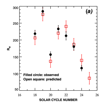
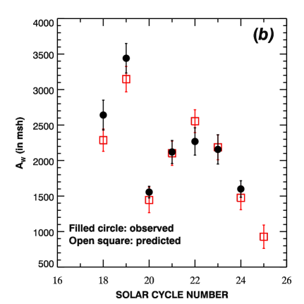
Figure 1: Hindsight: Comparison of the observed and the predicted values (a) of $R_{\rm M}$ and (b) of $A_{\rm W}$ of Solar Cycles 18–24. The predicted values of $R_{\rm M}$ and $A_{\rm W}$ of Solar Cycle 25 are also shown.

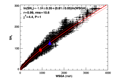
Figure 2: Scatter plot of the 13-month smoothed monthly mean area of sunspot groups in the Sun’s whole sphere (WSGA) versus the 13-month smoothed monthly mean ${\rm SN}_{\rm T}$ during the period 1874 – 2017 (1713 data points). The continuous curve (red) represents the linear least-squares best-fit to the $\ln({\rm WSGA})$ and $\ln({\rm SN}_{\rm T})$. The dotted curve (red) represents the one-rms level. The obtained linear equation and the values of the corresponding correlation coefficient $r$, rms, and $\chi^{2}$, and $P$ are given. The filled-triangle (blue) and filled-square (red) represent the predicted value of ${\rm SN}_{\rm T}$, i.e. $R_{\rm M}$ of Solar Cycle 25, by using the values of $A_{\rm W}$ of Solar Cycle 25 that are predicted using the $A_{\rm W}$–$W_{\rm M}$ relation in Javaraiah (2022) and $A^{*}_{\rm W}$–$W_{\rm W}$ relation above (cf. Table 2), respectively.

2 DATA AND ANALYSIS

Here have used monthly and 13-month smoothed monthly mean Version-2 international sunspot number (SN) during the period October 1874 – June 2017 (we downloaded the files SN_m_tot_v2.0.txt and SN_ms_tot_v2.0.txt from www.sidc.be/silso/datafiles). The details of changes and corrections in Version-2 SN can be found in Clette & Lefv́re (2016). We have used the values of the amplitudes ($R_{\rm M}$), i.e. the highest values of 13-month smoothed monthly mean sunspot numbers, and the maximum epochs ($T_{\rm M}$) of Sunspot Cycles 12 – 24 given by Pesnell (2018). Pesnell (2018) determined these from the time series of 13-month smoothed monthly mean values of SN. From the same time series we determined the epoch ($T_{\rm S}$) and the value of second largest peak ($S_{\rm M}$, say) during the maximum phase of each of Sunspot Cycles 12 – 24.

Recently, (Javaraiah, 2021), we analysed the daily sunspot-group data reported by the Greenwich Photoheliographic Results (GPR) during the period 1874 – 1976, Debrecen Photoheligraphic Data (DPD) during the period 1977 – 2017, and the revised Version-2 SN during the period 1874 – 2017. We determined the correlation of $R_{\rm M}$, $i.e.$ the amplitudes of Solar Cycles 13 – 24, with the sum of the areas of the sunspot groups in different $10^{\circ}$ latitude intervals and in different time intervals during Solar Cycles 12 – 23. We found that the sum of the areas ($A^{*}_{\rm R}$) of sunspot groups in $0^{\circ}-10^{\circ}$ latitude interval of the southern hemisphere during a small (7-month) interval just after one year from the maximum epoch of a solar cycle $n$ has a maximum correlation with $R_{\rm M}$ of the next solar cycle $n+1$. We derived the linear relationship between $A^{*}_{\rm R}(n)$ and $R_{\rm M}(n+1)$ by the method of linear least-square fit. By using the obtained $A^{*}_{\rm R}(n)-R_{\rm M}(n+1)$ linear relationship and $A^{*}_{\rm R}$ of Solar Cycle 24, we predicted the value $86\pm 18$ for $R_{\rm M}$ of Solar Cycle 25. Similarly, a prediction was also made for $A_{\rm W}$, i.e. the 13-month smoothed monthly mean areas of sunspot groups at $T_{\rm M}$ of a Solar Cycle 25. Here we check the consistency of the aforementioned method through hindsight of the $A^{*}_{\rm R}(n)-R_{\rm M}(n+1)$ relationship and also the $A^{*}_{\rm W}(n)-A_{\rm W}(n+1)$ relationship, where $A^{*}_{\rm W}(n)$ is the sum of the areas of the sunspot groups, determined similarly as $A^{*}_{\rm R}(n)$, well correlated with $A_{\rm W}(n+1)$.

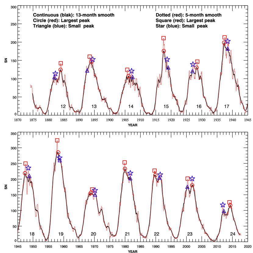
Figure 3: Variations in the 5-month (dotted-curve) and 13-month (continuous curve) smoothed monthly mean sunspot number (SN) during the period 1874 – 2017. The symbols circle (red) and triangle (blue) represent the largest and the second largest peaks of a sunspot cycle in the 13-month smoothed series. The corresponding peaks in 5-month smoothed series are represented by the symbols square (red) and star (blue), respectively. The Waldmeier solar cycle number is also given.

We find the existence of a high correlation and a good linear relationship between the cycle-to-cycle modulations in $R_{\rm M}$ and $S_{\rm M}$. By using this relation and the values predicted for $R_{\rm M}$ of Solar Cycle 25 by Javaraiah (2021, 2022) we predict the value of $S_{\rm M}$ of Solar Cycle 25. In Javaraiah (2022) we have calculated the least-square cosine fits to the cycle-to-cycle modulation in $R_{\rm M}$ during Solar Cycles 12 – 24. The same calculations are done here for $S_{\rm M}$. Since there is ambiguity in the positions of $S_{\rm M}$ of some cycles determined from the 13-month smoothed monthly mean SN series, hence we also determined 5-month smoothed monthly mean SN series and using it repeated all the calculations. In order to find that whether the peak of $R_{\rm M}$ or that of $S_{\rm M}$ would be first during the maximum of Solar Cycle 25, we fit cosine curves to the values of peaks that occurred first and second during the maxima of Solar Cycles 12 – 24.

Although it is well believed that the strength of polar magnetic fields at the end of a solar cycle is a good precursor for predicting the amplitude of the next solar cycle (Schtten et al., 1978; Svalgaard, Cliver, & Kamide, 2005), it is not clear yet exactly the time of polar fields which predict the amplitude. Therefore, the predicted amplitude of solar cycle has a considerable large uncertainty (Svalgaard, Cliver, & Kamide, 2005). Svalgaard, Cliver, & Kamide (2005) analysed the polar-fields data measured in Wilcox Observatory (WCO) and Mt. Wilson Observatory (MWO) during 1970 – 2005. They have used the average strength of dipole moment (DM: the average unsigned difference between the north and south polar fields) in the three years before the end of each of Solar Cycles 20 – 23 (one year in the case of Solar Cycle 23) for predicting the amplitude ($R_{\rm M}$) of Solar Cycle 24. Here we have analysed the polar-fields data measured in WCO and besides determining the average values of DM of the three years before the end of each of Solar Cycles 20 – 23, the average value of DM of the three years before the end of Solar Cycle 24 is determined. We have used the value of DM around the end, December/2019, of Solar Cycle 24. The WCO data are available at wso.stanford.edu/Polar.html are 30-day averages of the magnetic field measured in the polemost aperture calculated every 10 days. We have used the data that are corrected for the Earth’s rotational frequency. We have taken the corresponding average value of DM of Solar Cycle 20 from Table 1 in Jiang, Chatterjee, & Choudhuri (2007), it was determined from MWO data by Svalgaard, Cliver, & Kamide (2005). We determined correlation and linear least-square-fit to the values of DM and $A^{*}_{\rm R}$ of Solar Cycles 20 – 23. By using the obtained linear relationship first we predicted the average value of DM of the three years before the end of Solar cycle 24. We determined the correlation and the linear least-square fit of ${\rm DM}(n)$ and $R_{\rm M}(n+1)$, by using the values of DM of Solar Cycles 20 – 23 and the values of $R_{\rm M}$ of Solar Cycles 21 – 24. By substituting in the ${\rm DM}(n)-R_{\rm M}(n+1)$ relation the predicted and observed values of DM of Solar Cycle 24, we obtained the corresponding values for $R_{\rm M}$ of Solar Cycle 25. Finally we check the correlation between DM and $A^{*}_{\rm R}$ values of all five solar cycles.

Table 3: The epochs $T_{\rm M}$ and $T_{\rm S}$ of $R_{\rm M}$ and $S_{\rm M}$, respectively, of Sunspot Cycles 12 – 24 determined from 13-month smoothed monthly mean SN. The intervals (Gnevyshev gaps, in year) between these peaks, the ratios $S_{\rm M}$/$R_{\rm M}$, and the values of the mean and standard deviation of the absolute values of these parameters are also given.

$n$	$T_{\rm M}$	$R_{\rm M}$	$\sigma_{\rm M}$	$T_{\rm S}$	$S_{\rm M}$	$\sigma_{\rm S}$	$T_{\rm M}-T_{\rm S}$	$S_{\rm M}$/$R_{\rm M}$
12	1883.96	124.4	12.5	1881.96	104.1	11.5	$-$2.00	0.84
13	1894.04	146.5	10.8	1892.62	122.2	12.1	$-$1.42	0.83
14	1906.12	107.1	9.2	1907.45	104.6	9.1	1.33	0.98
15	1917.62	175.7	11.8	1919.04	130.6	10.2	1.42	0.74
16	1928.29	130.2	10.2	1926.96	120.8	9.8	$-$1.33	0.93
17	1937.29	198.6	12.6	1938.45	182.3	12.0	1.17	0.92
18	1947.37	218.7	10.3	1948.79	210.3	9.7	1.42	0.96
19	1958.20	285.0	11.3	1958.71	260.3	10.8	0.50	0.91
20	1968.87	156.6	8.4	1970.20	150.3	8.2	1.33	0.96
21	1979.96	232.9	10.2	1981.71	202.7	13.3	1.75	0.87
22	1989.87	212.5	12.7	1991.12	204.4	12.5	1.25	0.96
23	2001.87	180.3	10.8	2000.29	175.2	10.5	$-$1.58	0.97
24	2014.29	116.4	8.2	2012.21	98.3	7.5	$-$2.08	0.84
Mean		175.8	52.5		158.9	50.8	1.43$\pm$0.39	0.90$\pm$0.07

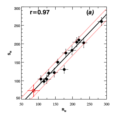
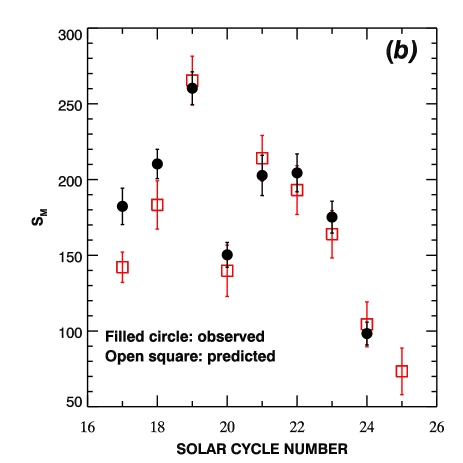
Figure 4: (a) Correlation between $R_{\rm M}$ and $S_{\rm M}$ (the values given Table 3) during Solar Cycles 12 – 24. The continuous line represents the best-fit linear relationship, Equation (1). The dotted lines (red) are drawn at one-rms level. (b) Hindsight: comparison of the observed and the predicted values of $S_{\rm M}$. The predicted value (red square) of $S_{\rm M}$ of Solar Cycle 25 is also shown in both (a) and (b) .

Table 4: Hindsight: The values of intercept ($C$) and slope ($D$) of the linear relationship between $R_{\rm M}$ and $S_{\rm M}$ correspond to the predictions for $S_{\rm M}$ of Solar Cycles 17 – 25. In the case of Solar Cycle $n=25$ the predicted value of $R_{\rm M}$ is used. The corresponding values of the correlation coefficient ($r$), $\chi^{2}$and its probability ($P$), number of data points ($N$), and predicted values of $S_{\rm M}$ are also given.

$n$	$C$	$D$	$r$	$\chi^{2}$	$P$	$N$	Pred.$S_{\rm M}$
17	$61.00\pm 30.46$	$0.41\pm 0.22$	0.89	0.81	0.85	5	$142.1\pm 10.0$
18	$14.23\pm 28.36$	$0.77\pm 0.19$	0.91	3.86	0.42	6	$183.2\pm 15.9$
19	$-12.75\pm 23.64$	$0.98\pm 0.15$	0.94	5.37	0.37	7	$265.3\pm 16.2$
20	$-9.62\pm 17.07$	$0.95\pm 0.09$	0.97	5.41	0.49	8	$139.8\pm 16.9$
21	$-6.97\pm 16.68$	$0.95\pm 0.09$	0.97	6.11	0.53	9	$214.0\pm 15.1$
22	$-4.67\pm 16.05$	$0.93\pm 0.09$	0.97	6.50	0.59	10	$193.1\pm 16.1$
23	$-5.98\pm 16.09$	$0.94\pm 0.09$	0.97	6.89	0.65	11	$163.9\pm 15.7$
24	$-5.79\pm 16.08$	$0.95\pm 0.09$	0.97	7.43	0.68	12	$104.4\pm 14.8$
25	$-9.54\pm 14.58$	$0.96\pm 0.08$	0.97	7.66	0.74	13	$73.4\pm 15.4$

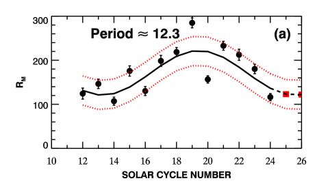
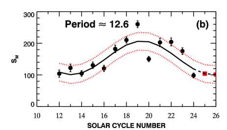
Figure 5: Continuous curve represents the best-fit cosine function to the values (filled circles) (a) of $R_{\rm M}$ and (b) of $S_{\rm M}$ of Sunspot Cycles 12 – 24 (for values in Table 3). The dotted curve (red) represents the one-rms level. The extrapolated portion is shown as a dashed curve and the filled squares (red) represent the predicted values of $R_{\rm M}$ and $S_{\rm M}$ of Sunspot Cycles 25 and 26. The period (in number of solar cycles) of the cosine function is also shown.

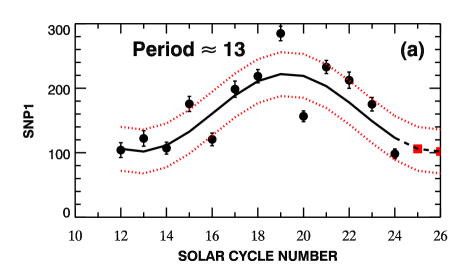
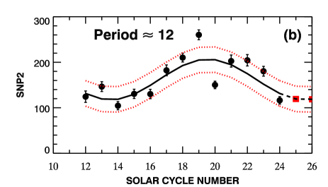
Figure 6: Continuous curve represents the best-fit cosine function to the values (filled circles) (a) of SNP1 and (b) of SNP2 of Sunspot Cycles 12 – 24 (for values in Table 5). The dotted curve (red) represents the one-rms level. The extrapolated portion is shown as a dashed curve and the filled squares (red) represent the predicted values of SNP1 and SNP2 of Sunspot Cycles 25 and 26. The period (in number of solar cycles) of the cosine function is also shown.

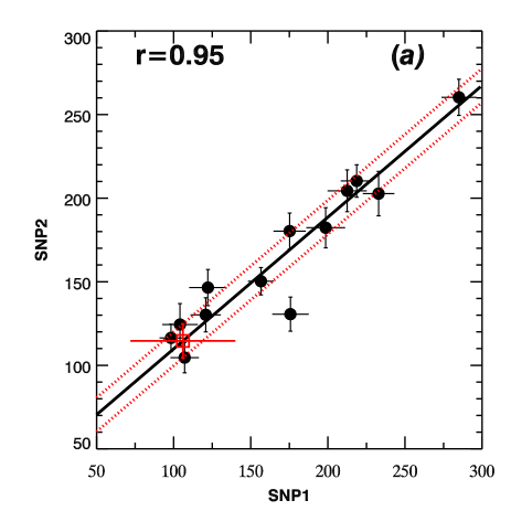
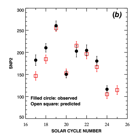
Figure 7: (a) Correlation between SNP1 and SNP2 during Solar Cycles 12 – 24. The continuous line represents the best-fit linear relationship, Equation (2). The dotted lines (red) are drawn at one-rms level. (b) Hindsight: comparison of the observed and the predicted values of SNP2. The predicted value of SNP2 of Solar Cycle 25 is also shown in both (a) and (b).

Table 5: The epochs TSN1 and TSN2 of the first peak (SNP1) and the second peak (SNP2), respectively, of Sunspot Cycles 12 – 24 (determined from 13-month smoothed monthly mean SN). The intervals (Gnevyshev gaps, in year) between these peaks, the ratios SNP1/SNP2, and the values of the corresponding mean and standard deviation are also given. The values of $R_{\rm M}$ are indicated with bold-font.

$n$	TSN1	SNP1	$\sigma_{1}$	TSN2	SNP2	$\sigma_{2}$	TSN2$-$TSN1	$\frac{\rm SNP1}{\rm SNP2}$
12	1881.96	104.1	11.5	1883.96	124.4	12.5	2.00	0.84
13	1892.62	122.2	12.1	1894.04	146.5	10.8	1.42	0.83
14	1906.12	107.1	9.2	1907.45	104.6	9.1	1.33	1.02
15	1917.62	175.7	11.8	1919.04	130.6	10.2	1.42	1.35
16	1926.96	120.8	9.8	1928.29	130.2	10.2	1.33	0.93
17	1937.29	198.6	12.6	1938.45	182.3	12.0	1.17	1.09
18	1947.37	218.7	10.3	1948.79	210.3	9.7	1.42	1.04
19	1958.20	285.0	11.3	1958.71	260.3	10.8	0.50	1.09
20	1968.87	156.6	8.4	1970.20	150.3	8.2	1.33	1.04
21	1979.96	232.9	10.2	1981.71	202.7	13.3	1.75	1.15
22	1989.87	212.5	12.7	1991.12	204.4	12.5	1.25	1.04
23	2000.29	175.2	10.5	2001.87	180.3	10.8	1.58	0.97
24	2012.21	98.3	7.5	2014.29	116.4	8.2	2.08	0.84
Mean		169.8	58.1		164.9	45.9	1.43$\pm$0.39	1.02$\pm$0.14

Table 6: Hindsight: The values of intercept ($C$) and slope ($D$) of the linear relationship between SNP1 and SNP2 correspond to the predictions for SNP2 of Solar Cycles 17 – 25. In the case of Solar Cycle $n=25$ the value of SNP1 predicted through the extrapolation of best fit cosine curve of SNP2 shown in Fig. 6(b) is used. The corresponding values of the correlation coefficient ($r$), $\chi^{2}$ and its probability ($P$), number of data points ($N$), and predicted values of SNP2 are also given.

$n$	$C$	$D$	$r$	$\chi^{2}$	$P$	$N$	Pred. SNP2
17	$89.32\pm 28.94$	$0.29\pm 0.23$	0.33	7.69	0.05	5	$146.6\pm 9.7$
18	$49.45\pm 23.99$	$0.62\pm 0.17$	0.76	9.84	0.04	6	$184.5\pm 9.5$
19	$26.73\pm 19.14$	$0.80\pm 0.12$	0.87	11.36	0.04	7	$254.6\pm 7.3$
20	$23.53\pm 14.57$	$0.82\pm 0.08$	0.94	11.42	0.08	8	$152.5\pm 10.0$
21	$23.01\pm 14.34$	$0.82\pm 0.08$	0.94	11.46	0.12	9	$215.0\pm 9.6$
22	$25.18\pm 13.87$	$0.81\pm 0.08$	0.94	11.96	0.15	10	$196.4\pm 11.1$
23	$24.36\pm 13.89$	$0.81\pm 0.08$	0.95	12.18	0.20	11	$166.9\pm 10.9$
24	$24.84\pm 13.91$	$0.82\pm 0.08$	0.94	13.04	0.22	12	$105.2\pm 10.0$
25	$31.07\pm 11.87$	$0.79\pm 0.07$	0.95	13.90	0.24	13	$114.6\pm 10.1$

3 RESULTS

3.1 Hindsight of $A^{*}_{\rm R}(n)$–$R_{\rm M}(n+1)$ and $A^{*}_{\rm W}(n)$–$A_{\rm W}(n+1)$ relationships

In Table 1 we have given that in intervals $T^{*}_{\rm M}$ and $T^{*}_{\rm W}$, i.e. 7 – 9 months intervals about one-year after the maximum epochs of solar cycles, the sums of the areas of sunspot groups during these intervals, $A^{*}_{\rm R}$ and $A^{*}_{\rm W}$ (normalized by 1000) in $0^{\circ}-10^{\circ}$ latitude intervals of the southern hemisphere during Solar Cycles 12 – 23 that have maximal correlations with $R_{\rm M}$ and $A_{\rm W}$, respectively, of the corresponding next solar cycles  (also see table 1 in Javaraiah, 2021). The values of $A^{*}_{\rm R}$ and $A^{*}_{\rm W}$ of Solar Cycle 24 that were used for predicting $R_{\rm M}$ and $A_{\rm W}$ of Solar Cycle 25 are also given. We made hindsight of the linear relationships between $A^{*}_{\rm R}(n)$ and $R_{\rm M}(n+1)$ and between $A^{*}_{\rm W}(n)$ and $A_{\rm W}(n+1)$. The corresponding details are given in Table 2. The hindsight is reasonably good. That is, except in the case of $R_{\rm M}$ of Solar Cycle 18, in the remaining all cases the correlation is statistically significant at a level above 95 % as indicated by Student’s t-test. In each case the linear-least-square best fit is good, i.e., the slope of each linear relation is considerably larger than its uncertainty ($\sigma$: standard deviation).

Fig. 1 shows the comparison of the observed and the predicted values of $R_{\rm M}$ and $A_{\rm W}$ of Solar Cycles 18 – 24. The uncertainties are rms (root-mean-square deviation) values. In this figure the predicted values of $R_{\rm M}$ and $A_{\rm W}$ of Solar Cycle 25 are also shown. As can be seen in this figure in both the cases of $R_{\rm M}$ and $A_{\rm W}$ there is a reasonably good agreement between the predicted and observed values (there exists significant correlation between the observed and predicted values). The agreement is much better in the case of $A_{\rm W}$ than that of $R_{\rm M}$. The property that the observed value of $A_{\rm W}$ of Solar Cycle 22 is larger than that of $A_{\rm W}$ of Cycle 21 is even present in the corresponding predicted values of $A_{\rm W}$. Since here the uncertainties (standard errors) in the values of $A_{\rm W}$ are taken care in the calculation of the linear least-square fit between $A^{*}_{\rm W}(n)$ and $A_{\rm W}(n+1)$, we obtained slightly higher value, 927 msh, for $A_{\rm W}$ of Solar Cycle 25 than that (701 msh) was found in Javaraiah (2021).

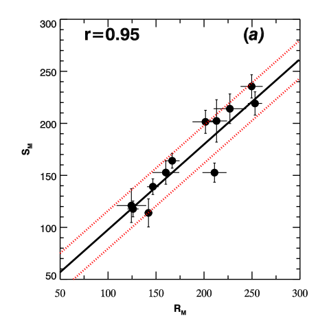
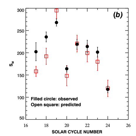
Figure 8: (a) Correlation between $R_{\rm M}$ and $S_{\rm M}$ during Solar Cycles 12 – 24 determined from the 5-month smooth monthly SN. The continuous line represents the best-fit linear relationship, Equation (3). The dotted lines (red) are drawn at one-rms level. (b) Hindsight: comparison of the observed and the predicted values of $S_{\rm M}$.

In many solar cycles there is no synchronize in the maxima of sunspot number and sunspot area. In Javaraiah (2022) we calculated the linear least-square fit to the 13-month smoothed monthly mean values of the area of the sunspot groups in the Sun’s whole sphere (WSGA) and total sunspot number (${\rm SN}_{\rm T}$). By using the predicted value of $A_{\rm W}$ from the $A_{\rm W}$–$W_{\rm M}$ relationship shown in that paper it was obtained $130\pm 12$ for $R_{\rm M}$ of Solar Cycle 25 ($W_{\rm M}$ is the maximum value of 13-month smoothed monthly mean area of sunspot groups in the Sun’s whole sphere during a solar cycle). However, since we have used the 13-month smoothed monthly mean values throughout the solar cycles, i.e. during maxima, minima, etc. of solar cycles, obviously, there exist considerable differences in the distributions of large and small sunspot groups during the solar cycles. It is well-known that the relationship between sunspot number and sunspot area is not strictly linear. Some scientists have shown that the size distribution of active regions is close to exponential (e.g. Tang, Howard, & Adkins, 1984). Some other scientists shown that it is close to power law or log-normal distribution (Bogdan et al., 1988; Harvey & Zwaan, 1993; Howard, 1996). Still some scientists have shown that the distribution of sunspot groups with respect to maximum area may not be fitted by a simple one-parameter distribution such as single power law or an exponential law (Gokhale & Sibaraman, 1981). Fig. 2 shows the plot of WSGA versus ${\rm SN}_{\rm T}$. As we can see in this figure, obviously the WSGA and ${\rm SN}_{\rm T}$ distribution is not exactly linear. The behavior of the beginning portion that correspond to the small values of WSGA is somewhat different from that of latter portion that correspond to the large values of WSGA. We calculated linear least-square fit to the logarithm values of WSGA and ${\rm SN}_{\rm T}$ and shown in Fig. 2. We find that uncertainty in this fit is considerably lower than that of the corresponding linear fit shown in Javaraiah (2022). A value $\approx 1348$  msh was obtained for $A_{\rm W}$ from the $A_{\rm W}$–$W_{\rm M}$ relationship (fig. 8 in Javaraiah (2022)). Here by using this value of $A_{\rm W}$ in the relationship shown in Fig. 2 we obtained $125\pm 11$ for $R_{\rm M}$ (it is nothing but ${\rm SN}_{\rm T}$ at $T_{\rm M}$) of Solar Cycle 25. It is slightly smaller than that was predicted earlier. By using $\approx$927  msh of $A_{\rm W}$ predicted from the $A^{*}_{\rm W}(n)$–$A_{\rm W}(n+1)$ relationship above, we obtained $92\pm 11$ for $R_{\rm M}$ of Solar Cycle 25. Both these predicted values are also shown in Fig. 2. The former is slightly larger–and the latter is slightly smaller–than the observed amplitude of Solar Cycle 24.

3.2 Prediction for strengths of double peaks of Solar Cycle 25

3.2.1 Prediction for the second maximum, $S_{\rm M}$

Fig. 3 shows the variations in the 13-month smoothed monthly mean sunspot number (SN) during the period 1874 – 2017. In this figure variations in the 5-month smoothed monthly SN is also shown. The values of the maximum ($R_{\rm M}$) and the second largest value ($S_{\rm M}$) of each of Sunspot Cycles 12 – 24 determined from in both these series are indicted. In Table 3 we have given the epochs $T_{\rm M}$ and $T_{\rm S}$ of $R_{\rm M}$ and $S_{\rm M}$, respectively, of Sunspot Cycles 12 – 24, determined from the 13-month smoothed data. The intervals (Gnevyshev gaps, in year) between these epochs, the values of the ratios of $S_{\rm M}$ to $R_{\rm M}$, and the values of the mean and the standard deviation of the corresponding absolute values are also given. As we can see in this table and in Fig. 3, in the case of Solar Cycles 12, 13, 16, 23, and 24 the second highest peaks occur first. The average size of the Gnevyshev gap is $\approx$1.4-year. In the case of Solar Cycle 19 the gap is relatively small (only 0.5-year). In fact, no significant Gnevyshev gap was identified in sunspot data of this cycle (e.g. Norton & Gallagher, 2010; Ravindra, Chowdhury, & Javaraiah, 2021). In the case of Solar Cycles 12 and 24 the gap is largest, about 2-year. The mean value of the ratio $S_{\rm M}/R_{\rm M}$ is 0.9 and the corresponding $\sigma$ is reasonably small. That is, the ratio is almost the same in most of the cycles. The ratio is somewhat small only in Solar Cycle 15 (there seems to be an ambiguity to identify the second highest peak).

Fig. 4(a) shows the correlation between $R_{\rm M}$ and $S_{\rm M}$ during Solar Cycles 12 – 24 (determined from the values in Table 3). The correlation is reasonably high (significant on 99 % confidence level). We calculated linear least-square fit by using the Interactive Digital Library (IDL) software FITEXY.PRO, downloaded from the website idlastro.gsfcnasa.gov/ftp/pro/math/. This software takes into account the errors in the values of both the abscissa and ordinate in the calculation of the linear least-square fit. Note that a small value of $P$ indicates a poor fit (large $\chi^{2}$). We obtained the following relationship:

$$S_{\rm M}=(-9.54\pm 14.58)+(0.96\pm 0.08)R_{\rm M}.$$ (1)

The least-square best fit is very good, i.e. the slope of this linear relationship is about 10 times larger than the corresponding $\sigma$. The $\chi^{2}=7.66$ is reasonably small and the corresponding probability (P = 0.74) is reasonably large. By using this relation and the predicted value $\approx 86$ ($\approx 92$) of $R_{\rm M}$ of Solar Cycle 25 we obtain $73\pm 15$ ($79\pm 15$) for $S_{\rm M}$ of Solar Cycle 25. The ratio $S_{\rm M}/$$R_{\rm M}$ of Solar Cycle 25 is 0.85, which is almost the same as that of Solar Cycle 24.

We did hindsight of the linear relationships between $R_{\rm M}$ and $S_{\rm M}$. The corresponding details are given in Table 4. The hindsight results are reasonably good in the sense that except in the case of Solar Cycles 17 and 18, in the remaining all cases the correlation is statistically significant and in each case the best-fit linear relationship is good. Fig. 4(b) shows the comparison of the observed and the predicted values of $S_{\rm M}$ of Solar Cycles 17 –2̇4. In this figure the predicted values of $S_{\rm M}$ of Solar Cycle 25 are also shown. As can be seen in this figure, except in the case of Solar Cycles 17 and 18, in the remaining all solar cycles there is a reasonable good agreement between the predicted and the observed values.

In Fig. 5 we compare the best-fit cosine curves of $R_{\rm M}$ (the same as shown in fig. 7 of Javaraiah, 2022) and $S_{\rm M}$ during Solar Cycles 12 – 24. The corresponding values of $\chi^{2}$ are 155 and 104, respectively. As we can see in this figure the cosine best fits of both $R_{\rm M}$ and $S_{\rm M}$ mostly the same (periods are almost equal). The extrapolations of these curves yield $123\pm 33$ for $R_{\rm M}$ and $104\pm 28$ for $S_{\rm M}$ of Solar Cycle 25. The aforementioned predictions are based on a model where the $\chi^{2}$ is large ($>100$) and are thus not particularly reliable. A wide range of lengths (60 – 140 years) are suggested for Gleissberg cycle (e.g. Ogurtsov et al., 2002). The size (143 years) of the data used here is not adequate to determine precisely the long-term periodicity in solar activity. In Fig. 5, there is an indication of the predicted values of $R_{\rm M}$ and $S_{\rm M}$ are at the minimum of upcoming long-period cycle. However, this conclusion is not supported by the observations at a statistically significant level (i.e. the null case is not excluded at the 5 % level).

3.2.2 Prediction for first and second peaks (irrespective of heights)

As we have noticed above in some solar cycles the peak of $R_{\rm M}$ occurred first and in some other solar cycles the peak of $S_{\rm M}$ occurred first (see Fig. 3, Table 3). In the above analysis (Sec. 3.2.1) it is not possible to predict whether the peak of $R_{\rm M}$ or that of $S_{\rm M}$ will occur first during the maximum of Solar Cycle 25. This is because the peaks of $R_{\rm M}$ and $S_{\rm M}$ are not in the same chronological order in all solar cycles. Therefore, the information on the order of occurrence of $R_{\rm M}$ and $S_{\rm M}$ in solar cycles is not given in Table 3. However, it is not required for the purpose of that analysis. We reorganized the data given in Table 3 according to the order of occurrence of the peaks that correspond to $R_{\rm M}$ and $S_{\rm M}$. Table 5 contains the reorganized data, i.e. in this table we gave the epochs TSN1 and TSN2 of the first peak (SNP1) and the second peak (SNP2), respectively, during the maxima of Sunspot Cycles 12 – 24. It should be noted that both the data of SNP1 and SNP2 contain the values of $R_{\rm M}$ of some cycles and of $S_{\rm M}$ of some other cycles. In Table 5 the values of $R_{\rm M}$ are indicated with bold-font. The intervals (Gnevyshev gaps, in year) between these peaks, i.e TSN2$-$TSN1, the ratios of SNP1 to SNP2, and the values of the corresponding mean and standard deviation are also given. As can be seen in this table the data of SNP1 contain the values of $R_{\rm M}$ of Solar Cycles 14 – 15 and 17 – 18 and the values of $S_{\rm M}$ of Solar Cycles 12, 13 , 16, 23, and 24. Obviously, the data of SNP2 contain the values of $S_{\rm M}$ of the former cycles and the values of $R_{\rm M}$ of latter cycles. There is no significant difference between the average values SNP1 and SNP2 (almost the same). Obviously, the average size of the Gnevyshev gap is the same as given in Table 3. The average value of the ratio SNP1/SNP2 is about one. Solar Cycles 12 and 24 have the same value of the ratio SNP1/SNP2 and almost the same size of Gnevyshev gap. In fact, it seems when SNP2 is larger than SPN1, i.e. when SPN2 represents $R_{\rm M}$, the corresponding Gnevyshev gap is relatively large, the peaks are well separated, both peaks are well defined (except in Solar Cycle 13) and SNP1/SNP2 ratio is to some extent small. In addition, the corresponding solar cycles might be relatively small (probably smaller than the respective preceding solar cycles). All these characteristics also support for a small Solar Cycle 25 and it would have a large Gnevyshev gap similar to those of Solar Cycles 12 and 24. In each hemisphere the temporal behavior of the activity in Solar Cycles 24 is almost the same as that of Solar Cycle 12 and in both of these solar cycles the peak of whole sphere activity depict the dominant peak of activity in southern hemisphere (see fig.1 in Javaraiah, 2020). In fact, some authors reported that Solar Cycles 12 and 24 are as similar (in shape) cycles (Du, 2020).

Fig. 6 shows the cosine fits to the values of SNP1 and SNP2 during Solar Cycles 12 – 24. The corresponding values of $\chi^{2}$ are 141 and 110, respectively. As we can see in this figure the best fit cosine functions of SNP1 and SNP2 have periods $\approx$13-cycle and $\approx$12-cycle, respectively. That is, the period of SNP1 is about one-cycle period (11-year) larger than that of SNP2, and obviously SNP1 leads SNP2 by about one year (note that the average size of Gnevyshev gap is about one-year). These results may be somewhat consistent with the superimposition of two waves of solar activity with some phase difference could be a cause for the dual-peaks in the maxima of solar cycles as suggested by Gnevyshev (1967, 1977). However, Gnevyshev (1967, 1977) suggested superimposition of two $\approx$11-year period waves, whereas the aforementioned result suggests superimposition of two waves of periods $\approx$12-cycle and $\approx$13-cycle. The extrapolations of the cosine curves of SNP1 and SNP2 yield $106\pm 34$ and $119\pm 28$ for SNP1 and SNP2, respectively, of Solar Cycle 25. These predictions are not particularly reliable because the $\chi^{2}$ of the fit is large ($>100$). However, form this analysis by a large extent clear that like in Solar Cycle 24, in Solar Cycle 25 the second peak would be larger than first peak. Obviously, the values of the large and the small peaks represent $R_{\rm M}$ and $S_{\rm M}$, respectively. The ratio SNP1/SNP2 of Solar Cycle 25 is about 0.89, which is only slightly larger than that of Solar Cycle 24 (see Table 5). In general, all the inferences drawn from the best fit cosine functions have no statistical support, hence they are at best only suggestive rather than compelling.

Fig. 7(a) shows the correlation between SNP1 and SNP2 during Solar Cycle 12 – 24. This correlation ($r=0.95$) is considerably smaller than that of between $R_{\rm M}$ and $S_{\rm M}$ shown in Fig. 4(a), but still statically significant ($P=0.05$). We obtained the following relationship between SNP1 and SNP2 by using the values of these parameters given in Table 5:

$${\rm SNP2}=(31.07\pm 11.87)+(0.79\pm 0.07){\rm SNP1}.$$ (2)

The least-square best fit of this relation of SNP1 and SNP2 is good, i.e, the slope is about 11 times larger than the corresponding standard deviation. In this relation by using the value of SNP1 of Solar Cycle 25 predicted above by extrapolating the best-fit cosine curve of SNP1 shown in Fig. 5(a) we get $114.6\pm 10.1$ for SNP2 of Solar Cycle 25. It is not significantly different from the one predicted from the cosine fit of NSP2. As we can see in Table 6 (after Solar Cycle 18) and in Fig. 7(b) the hindsight of this relationship suggests a reasonable consistency in the SNP1–SNP2 relationship and the corresponding prediction is reasonably reliable.

3.3 Analysis of 5-month smoothed monthly mean SN

Since in our earlier analyses we have predicted 13-month smoothed monthly mean values of the amplitude of Solar Cycle 25, in order to use that predicted values here (in Sec. 3.2) we have analysed the 13-month smoothed data of SN. Some solar cycles contain more peaks during their maxima. We considered only the two peaks which are higher than remaining ones. In general there are some solar cycles in which there is a difficulty to identify Gnevyshev gaps, for example, Solar Cycles 13, 15, and 19 in 13-month smoothed monthly mean values of SN. Therefore, here we also analyse the data in relatively short intervals: 5-month smoothed monthly mean SN data. In this data the Gnevyshev peaks are relatively well defined compared to the corresponding peaks in the 13-month smoothed data (see Fig. 3). The epochs of the peaks during many solar cycles in the 13-month smoothed data closely match with the corresponding peaks in the 5-month smoothed data. However, there is an ambiguity in determining from the 13-month smoothed data the epochs of $R_{\rm M}$ and $S_{\rm M}$ of some solar cycles. For example, in the case of Solar Cycles 13 and 15 the positions of the peaks of $S_{\rm M}$ in the 13-month smoothed series are seem to be in a large extent different in the 5-month smoothed series. In the case of Solar Cycle 19 there is peak of $S_{\rm M}$ in the 5-month smoothed data, but it is washed out in the 13-month smoothed data (except that there is a slight signal of it). In the case of a few solar cycles $R_{\rm M}$ is first and $S_{\rm M}$ is second in the 13-month smooth data, whereas it is opposite in the 5-month smoothed data: for example, Solar Cycles 13 and 23. In Solar Cycle 23 the values $R_{\rm M}$ and $S_{\rm M}$ are almost equal in the 5-month smoothed data.

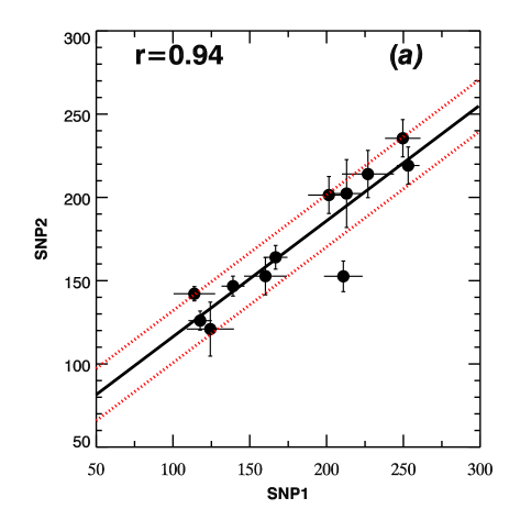
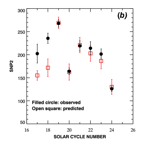
Figure 9: (a) Correlation between SNP1 and SNP2 during Solar Cycles 12 – 24 determined from 5-month smooth monthly SN. The continuous line represents the best-fit linear relationship, Equation (4). The dotted lines (red) are drawn at one-rms level. (b) Hindsight: comparison of the observed and the predicted values of SNP2.

Tables 7, 8, 9, and 10 are obtained from the 5-month smoothed data similarly as Tables 3, 4, 5, and 6, respectively, that were obtained from the 13-month smoothed data. Figs. 8 and 9 are obtained from the 5-month smoothed data similarly as Figs. 4 and 7, respectively, that were obtained from the 13-month smoothed data. Obviously, there are considerable differences between the sizes of Gnevyshev gaps of many solar cycles determined from the 5-month and 13-month smoothed data, though the the corresponding all cycles’ average sizes are equal. In Solar Cycles 13 and 23 the values of Gnevyshev gaps even have opposite signs (see Tables 3 and 7). There are significant differences in the values of $S_{\rm M}/R_{\rm M}$ of solar Cycles 13, 19, and 24 determined from the 5-month and 13-month smoothed data. The corresponding over all cycles’ average values are almost equal. Similar arguments can be made by comparing the values of SNP1 and SNP2 derived from 5-month and 13-month smoothed data (see Tables 5 and 9).

By using the values of $R_{\rm M}$ and $S_{\rm M}$ given in Table 7 we obtained the following relationship:

$$S_{\rm M}=(15.86\pm 13.62)+(0.82\pm 0.07)R_{\rm M}.$$ (3)

The least-square best-fit of Equation (3) by a large extent is good as that of Equation (1) that derived from the values of 13-month smoothed data. The parameters of Equation (3) are also given in Table 8. The slope of this linear relationship is about 11.7 times larger than the corresponding $\sigma$. The $\chi^{2}=14.8$ is reasonably smaller than 5% significant level (i.e. P = 0.19 is much larger than 0.05).

We obtained the following relationship between SNP1 and SNP2 by using the values of these parameters given in Table 10:

$${\rm SNP2}=(31.07\pm 11.87)+(0.79\pm 0.07){\rm SNP1}.$$ (4)

The least-square best fit of this relation of SNP1 and SNP2 is also reasonably good. The parameters of Equation (4) are also given in Table 8. The slope is about 11.3 times larger than the corresponding $\sigma$. The $\chi^{2}=16.4$ is to some extent smaller than 5% significant level (i.e. P = 0.13 is significantly larger than 0.05).

The hindsight of Equations (3) and (4) is shown in Tables 9 and 10 and in Figs. 8(b) and 9(b). As can be seen in these tables and figures there exists a reasonable consistency in predictions made (for Solar Cycle 19 – 24) by using these relations. Earlier the 5-month smoothed value of $R_{\rm M}$ of Solar Cycle 25 was not predicted. Hence, here the 5-month smoothed value of $S_{\rm M}$ can not be predicted. We did cosine fits to the 5-month smoothed values of $R_{\rm M}$ and $S_{\rm M}$ (not shown here). Although we find the values of $R_{\rm M}$ and $S_{\rm M}$ of Solar Cycle 25 are similar to those obtained from the cosine fits shown in Fig. 5 for 13-month smoothed data, the $\chi^{2}$ values of the corresponding best fits are found to be relatively large. Hence, here we have not used them.

Overall, by analyzing the 5-month smoothed data we confirmed that there is a reasonable consistency in the results derived from the 13-month smoothed data. That is, although, obviously, there are significant differences in the Gnevyshev gaps of some solar cycles determined from the 5-month and the 13-month smoothed data, they may not have a significant impact on the values of $S_{\rm M}$ predicted above by using the 13-month smoothed data.

Table 7: The epochs $T_{\rm M}$ and $T_{\rm S}$ of $R_{\rm M}$ and $S_{\rm M}$, respectively, of Sunspot Cycles 12 – 24 determined from the 5-month smoothed monthly mean SN. The intervals (Gnevyshev gaps, in year) between these peaks, the ratios $S_{\rm M}$/$R_{\rm M}$, and the values of the mean and standard deviation of the absolute values of these parameters are also given.

$n$	$T_{\rm M}$	$R_{\rm M}$	$\sigma_{\rm M}$	$T_{\rm S}$	$S_{\rm M}$	$\sigma_{\rm S}$	$T_{\rm M}-T_{\rm S}$	$S_{\rm M}$/$R_{\rm M}$
12	1884.04	142.1	4.3	1882.29	113.9	13.5	$-$1.75	0.80
13	1893.45	160.2	13.9	1894.45	152.7	11.2	1.00	0.95
14	1905.71	124.3	15.4	1907.12	120.9	16.2	1.42	0.97
15	1917.54	210.9	12.5	1918.71	152.6	9.2	1.17	0.72
16	1928.54	146.7	6.0	1927.12	139.1	7.5	$-$1.42	0.95
17	1937.45	213.0	11.0	1938.45	202.3	20.4	1.00	0.95
18	1947.54	249.6	11.5	1948.46	235.5	11.2	0.92	0.94
19	1957.87	323.5	13.4	1958.62	267.9	8.0	0.75	0.83
20	1969.29	166.8	7.7	1970.20	164.0	7.1	0.92	0.98
21	1979.87	253.1	7.4	1981.71	219.1	11.2	1.83	0.87
22	1989.62	226.9	16.9	1991.45	214.0	14.2	1.83	0.94
23	2000.37	201.5	13.5	2001.87	201.4	11.1	1.50	1.00
24	2014.04	126.0	5.7	2011.87	117.7	7.6	$-$2.17	0.93
Mean		195.7	58.7		177.0	49.6	1.34$\pm$0.44	0.91$\pm$0.08

Table 8: Hindsight: The values of intercept ($C$) and slope ($D$) of the linear relationship between $R_{\rm M}$ and $S_{\rm M}$ correspond to the predictions for $S_{\rm M}$ of Solar Cycles 17 – 25 (5-month smoothed monthly values). The corresponding values of the correlation coefficient ($r$), $\chi^{2}$ and its probability ($P$), number of data points ($N$), and predicted values of $S_{\rm M}$ are also given.

$n$	$C$	$D$	$r$	$\chi^{2}$	$P$	$N$	Pred.$S_{\rm M}$
17	$81.84\pm 30.27$	$0.36\pm 0.19$	0.74	3.82	0.28	5	$158.2\pm 11.6$
18	$49.68\pm 38.95$	$0.57\pm 0.23$	0.83	7.07	0.13	6	$192.0\pm 18.3$
19	$-7.18\pm 27.88$	$0.93\pm 0.15$	0.91	9.18	0.10	7	$294.9\pm 18.0$
20	$12.35\pm 16.73$	$0.81\pm 0.08$	0.95	10.22	0.12	8	$148.0\pm 22.3$
21	$18.54\pm 16.24$	$0.80\pm 0.08$	0.95	12.44	0.09	9	$220.6\pm 19.0$
22	$19.00\pm 15.39$	$0.80\pm 0.07$	0.95	12.45	0.13	10	$199.4\pm 20.0$
23	$17.96\pm 15.55$	$0.80\pm 0.07$	0.95	12.97	0.16	11	$179.9\pm 19.8$
24	$17.54\pm 15.77$	$0.81\pm 0.08$	0.94	14.76	0.14	12	$119.9\pm 18.7$
25	$15.86\pm 13.62$	$0.82\pm 0.07$	0.95	14.80	0.19	13	–

Table 9: The epochs TSN1 and TSN2 of the first peak (SNP1) and the second peak (SNP2), respectively, of Sunspot Cycles 12 – 24 determined from the 5-month smoothed monthly mean SN. The intervals (Gnevyshev gaps, in year) between these peaks, the ratios SNP1/SNP2, and the values of the corresponding mean and standard deviation are also given. The values of $R_{\rm M}$ are indicated with bold-font.

$n$	TSN1	SNP1	$\sigma_{1}$	TSN2	SNP2	$\sigma_{2}$	TSN2$-$TSN1	$\frac{\rm SNP1}{\rm SNP2}$
12	1882.29	113.9	13.5	1884.04	142.1	4.3	1.75	0.80
13	1893.45	160.2	13.9	1894.45	152.7	11.2	1.00	1.05
14	1905.71	124.3	15.4	1907.12	120.9	16.2	1.42	1.03
15	1917.54	210.9	12.5	1918.71	152.6	9.2	1.17	1.38
16	1927.12	139.1	7.5	1928.54	146.7	6.0	1.42	0.95
17	1937.45	213.0	11.0	1938.45	202.3	20.4	1.00	1.05
18	1947.54	249.6	11.5	1948.46	235.5	11.2	0.92	1.06
19	1957.87	323.5	13.4	1958.62	267.9	8.0	0.75	1.21
20	1969.29	166.8	7.7	1970.20	164.0	7.1	0.92	1.02
21	1979.87	253.1	7.4	1981.71	219.1	11.2	1.83	1.16
22	1989.62	226.9	16.9	1991.45	214.0	14.2	1.83	1.06
23	2000.37	201.5	13.5	2001.87	201.4	11.1	1.50	1.00
24	2011.87	117.7	7.6	2014.04	126.0	5.7	2.17	0.93
Mean		192.3	62.64		180.4	45.8	1.36$\pm$0.44	1.05$\pm$0.14

Table 10: Hindsight: The values of intercept ($C$) and slope ($D$) of the linear relationship between SNP1 and SNP2 correspond to the predictions for SNP2 of Solar Cycles 17 – 25 (5-month smoothed monthly values). The corresponding values of the correlation coefficient ($r$), $\chi^{2}$ and its probability ($P$), number of data points ($N$), and predicted values of SNP2 are also given.

$n$	$C$	$D$	$r$	$\chi^{2}$	$P$	$N$	Pred. SNP2
17	$126.19\pm 16.34$	$0.14\pm 0.11$	0.62	2.15	0.54	5	$155.0\pm 10.5$
18	$113.80\pm 19.40$	$0.23\pm 0.12$	0.76	6.59	0.16	6	$171.7\pm 19.2$
19	$48.78\pm 22.50$	$0.68\pm 0.13$	0.87	14.86	0.01	7	$269.1\pm 12.3$
20	$49.67\pm 13.75$	$0.68\pm 0.07$	0.94	14.86	0.02	8	$162.3\pm 17.6$
21	$50.22\pm 13.35$	$0.67\pm 0.07$	0.94	14.89	0.04	9	$220.8\pm 16.6$
22	$50.59\pm 12.82$	$0.67\pm 0.06$	0.94	14.90	0.06	10	$202.9\pm 17.3$
23	$49.94\pm 12.92$	$0.68\pm 0.06$	0.94	15.25	0.08	11	$186.4\pm 17.1$
24	$49.70\pm 12.95$	$0.68\pm 0.06$	0.94	16.27	0.09	12	$130.1\pm 16.2$
25	$46.72\pm 11.26$	$0.70\pm 0.06$	0.94	16.45	0.13	13	–

Table 11: DM (in $\mu$Tesla) and $\sigma_{\rm DM}$ (in $\mu$Tes) represent the average dipole moment in the 3-year interval $T^{*}_{\rm DM}$ just before the end of a solar cycle and the corresponding uncertainty, respectively, determined from Wilcox Observatory polar fields data for Solar Cycles 21 – 24 and it is taken from the paper by Jiang et. al (2007) for Solar Cycle 20 ($\sigma_{\rm DM}$ is not available), which was determined from MWO polar fields data by Svalgaard, Cliver, & Kamide (2005). The symbol ^a indicates the average $\sigma_{\rm DM}$ of Cycles 21 – 24.

$n$	$T^{*}_{\rm DM}$	DM	$\sigma_{\rm DM}$
20	1973.21-1976.21	250	1.4a
21	1983.71-1986.71	247.8	2.7
22	1993.62-1996.62	200.3	1.2
23	2005.96-2008.96	112.9	0.9
24	2016.96-2019.96	125.8	0.8

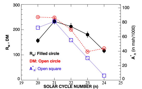
Figure 10: Variations in average dipole moment (DM) over last 3 years of solar cycles, the sum ($A^{*}_{\rm R}$) of the areas of sunspot groups in $0^{\circ}-10^{\circ}$ latitude during a small (7 months) interval just after the maxima of solar cycles, and the amplitude ($R_{\rm M}$, maximum yearly mean value of sunspot number) of the solar cycle. In the case of $R_{\rm M}$ and DM the error bars are $1\sigma$ (standard deviation) levels (the error in a value of DM is very small).

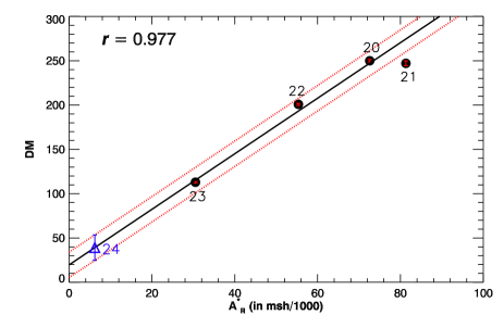
Figure 11: The scatter plot of $A^{*}_{\rm R}$ versus DM of Solar Cycles 20 – 23. The continuous line represents the best-fit linear relation, Equation (5) and dotted curves represent one-rms. The corresponding value of the correlation-coefficient ($r$) is given and Waldmeier solar solar cycle number is also shown. The triangle (blue) represents the derived strength of the average DM of 3 years before the end of Solar Cycle 24.

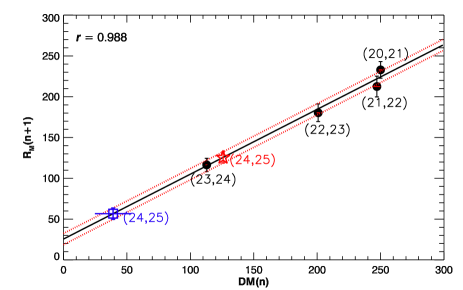
Figure 12: Plot of DM ($n$) versus $R_{\rm M}$ ($n+1$), where $n=20,\dots,23$ represents the Waldmeier solar cycle number. The continuous line represents the best fit linear relationship, Equation (6) and the dotted curves represent one-rms level. The corresponding value of $r$ is given and the pairs of Waldmeier solar solar cycle numbers are also shown. The symbol star (red) represents the $R_{\rm M}$ of Solar Cycle 25 predicted by substituting in Equation (6) the observed mean value of DM. The symbol square (blue) represents the value that obtained by substituting in Equation (6) the predicted average value of DM over last 3-years of Solar Cycle 24.

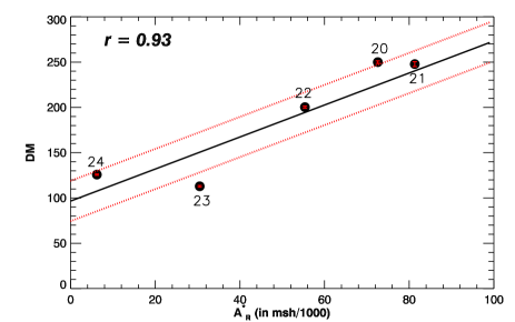
Figure 13: The scatter plot of $A^{*}_{\rm R}$ versus DM of Solar Cycles 20 – 24. The continuous line represents the best-fit linear relation and the dotted curves represent one-rms level. The corresponding value of $r$ is given and Waldmeier solar solar cycle number is also shown. This figure is the same as Fig. 9, but the observed value of DM of Solar Cycle 24 is included.

3.4 Comparison between $A^{*}_{\rm R}$ and DM

In Table 11 we have given the values of DM of Solar Cycles 20–24. Fig. 10 shows the cycle-to-cycle variations in $R_{\rm M}$, $A^{*}_{\rm R}$, and DM during Solar Cycles 20–24 (the error in DM is very small). As can be seen in this figure the profiles of all these parameters are closely similar. However, the pattern of DM of all the five solar cycles, 20–24, is somewhat different. $A^{*}_{\rm R}$ is considerably decreased from Solar Cycle 23 to Solar Cycle 24. In fact, $A^{*}_{\rm R}$ monotonically decreased from Solar Cycle 21 to Solar Cycle 24. DM also decreased from Solar Cycle 21 to Solar Cycle 23, but slightly increased from Solar Cycle 23 to Solar Cycle 24.

Fig. 11 shows the scatter plot of $A^{*}_{\rm R}$ versus DM during Solar Cycle 20 – 23. The corresponding correlation ($r=0.98$) is very good, $i.e.$ it is statistically highly significant (Student’s $t=6.5$, $t=4.3$ for $p=0.05$ for 2 degree of freedom). We obtained the following linear relationship between $A^{*}_{\rm R}$ and DM during Solar Cycles 20 – 23:

$${\rm DM}=(19.7\pm 1.7)+(3.1\pm 0.3)A^{*}_{\rm R}.$$ (5)

The uncertainties (see Table 11) in the value of DM are taken care in the least-square fit calculations. The best-fit linear relation is reasonably good, $i.e.$ the slope is about ten times larger than the corresponding $\sigma$. $\chi^{2}=3.1$ is reasonably small (note that $\chi^{2}=7.815$ for $p=0.05$ for 3 degree of freedom). Except the data point of Solar Cycle 21, the remaining three data points are laying within one-rms level. In Equation (5) by substituting the value of $A^{*}_{\rm R}$ (given in Table 1) of Solar Cycle 24, we obtained $39\pm 14$ for DM of Solar Cycle 24 (${\rm rms}=14$ looks to be relatively large, but this predicted value of DM is close to the lower end of the large range of DM values). This predicted value of DM of Solar Cycle 24 is also shown in Fig. 11.

Fig. 12 shows the scatter plot of DM(n) versus $R_{\rm M}$ (n+1), where $n=20,\dots,23$ represents the Waldmeier solar cycle number. The corresponding correlation ($r=0.99$) is statistically highly significant (Student’s $t=9.1$). We obtained the following linear relationship:

$$R_{\rm M}(n+1)=(25\pm 18)+(0.79\pm 0.08){\rm DM}(n).$$ (6)

The uncertainties of both DM and $R_{\rm M}$ are taken care in this linear least-square fit calculations. The least-square fit to the data is reasonably good, $i.e.$ $\chi^{2}=1.47$ is small and the corresponding $P=0.48$ (the $\chi^{2}$ is considerably smaller than 5 % confidence level). The rms$=6.9$ is also considerably small and almost all the data points are within the one-rms level. In Equation (6) by substituting the predicted and observed (see Table 11) values of DM of Solar Cycle 24, we obtained the values $57\pm 7$ and $125\pm 7$, respectively, for $R_{\rm M}$ of Solar Cycle 25. These predicted values are also sown in Fig. 12. The latter and the value predicted from WSGA–$\rm{SN}_{\rm T}$ relationship (shown in Fig. 2) above, are agree each other very well. However, the value ($86\pm 18$) is predicted for $R_{\rm M}$ of Solar Cycle 25 in Javaraiah (2021) by using $A^{*}_{\rm R}(n)$–$R_{\rm M}(n+1)$ linear relationship is much higher than the former and considerably lower than the latter. The predicted value for $R_{\rm M}$ of Solar Cycle 25 by using the observed value of DM is substantially (about 119 %) larger than that predicted by using the predicted value of DM. The former is slightly larger–whereas the latter is substantially lower–than the value of $R_{\rm M}$ of Solar Cycle 24.

Since the corresponding correlations of both the $A^{*}_{\rm R}(n)$ – $R_{\rm M}(n+1)$ and ${\rm DM}(n)$–$R_{\rm M}(n+1)$ (Equation (6)) linear relationships are high, hence we can expect a reasonable high correlation between $A^{*}_{\rm R}$ and DM. Fig. 13 shows the correlation between $A^{*}_{\rm R}$ and DM determined from the values of all the five pairs of data of Solar Cycles 20 – 24. The correlation ($r=0.93$) is larger than that of 5 % significant level (Student’s $t=4.5$), but substantially lower than that determined from the four pairs of data of Solar Cycles 20 – 23 shown in Fig. 11. $\chi^{2}=15.7$ is much larger then that $\chi^{2}=9.488$ of 5 % significant level for four degrees of freedom and ${\rm rms}=22.2$ is also relatively large. That is, in this case there is a relatively large scatter in the data points.

Overall, the value of DM predicted for Solar Cycle 24 is much smaller than the observed one (see Table 11). Obviously, the predicted value of DM is incorrect. Therefore, the predicted value of $R_{\rm M}$ of Solar Cycle 25 by using the predicted value of DM of Solar Cycle 24 is also incorrect. In addition, the correlation between $A^{*}_{\rm R}$ and DM determined from the values of all the five pairs of data of Solar Cycles 20 – 24 is weak. All these imply that there exists only a weak relationship between $A^{*}_{\rm R}$ and DM in Solar Cycle 24.

4 DISCUSSION AND CONCLUSIONS

In a series of papers, we predicted the amplitudes of Solar Cycles 24 and 25 by using the linear relationship between $A^{*}_{\rm R}$ of a solar cycle (n) and $R_{\rm M}$ of the next solar cycle (n+1). In the present analysis by verifying the $A^{*}_{\rm R}(n)$–$R_{\rm M}(n+1)$ and $A^{*}_{\rm W}(n)$–$A_{\rm W}(n+1)$ relationships through hindsight we confirmed that there is a good consistency in this method of prediction for the amplitude of a solar cycle. From this method a value $86\pm 18$ ($92\pm 11$) is predicted for $R_{\rm M}$ of Solar Cycle 25 (Javaraiah, 2021). Recently, by fitting a cosine function to the cycle-to-cycle modulations in the maxima of the mean area of sunspot groups of Solar Cycles 12 – 24 and using the existence of a reasonably good linear relationship between the long-term variations of sunspot-group area and sunspot number we predicted $130\pm 12$ for $R_{\rm M}$ of Solar Cycle 25 (Javaraiah, 2022). In the present analysis we have made an improvement in the relationship between long-term variations of sunspot number and sunspot-group area, Therefore, the aforementioned prediction is found to be $125\pm 11$. We show the existence of a good correlation between the strength of polar fields (DM) at the end of a solar cycle $n$ and the amplitude ($R_{\rm M}$) of solar cycle $n+1$. We predicted $R_{\rm M}$ of Solar Cycle 25 by using the strength of polar fields (DM) at the end of Solar Cycle 24. We found $125\pm 7$ for $R_{\rm M}$ of Solar Cycle 25. This and the value $125\pm 11$ predicted from the aforementioned previous method agree each other very well, but considerably larger than the value predicted by using the $A^{*}_{\rm R}(n)$–$R_{\rm M}(n+1)$ relationship.

We find that there exits a good correlation between $R_{\rm M}$ and $S_{\rm M}$ during the Solar Cycles 12 – 24. By using the predicted value $\approx 86$ ($\approx 92$) of $R_{\rm M}$ of Solar Cycle 25 and the $R_{\rm M}$–$S_{\rm M}$ linear relation we predict $73\pm 15$ ($79\pm 15$) for $S_{\rm M}$ of Solar Cycle 25. The value 0.85 of the ratio $S_{\rm M}$/$R_{\rm M}$ of Solar Cycle 25 is found to be almost the same as that of Solar Cycle 24. The cosine fits to the values of the first and the second peaks (irrespective of their heights) of Solar Cycles 12 – 24 suggest the existence of $\approx$13-cycle and $\approx$12-cycle periods in the variations of the first and second peak values, respectively. Moreover, from this analysis we find that in Solar Cycle 25 $S_{\rm M}$ would occur before $R_{\rm M}$, the same as in Solar Cycle 24. However, this analysis suggests $\approx$106 and $\approx$119 for $S_{\rm M}$ and $R_{\rm M}$ of Solar Cycle 25, respectively. Since in our earlier analyses we have predicted 13-month smoothed monthly mean values of the amplitude of Solar Cycle 25, in order to use them here we have analysed the 13-month smoothed data of SN to determine the Gnevyshev gaps. However, through the analysis of the data in relatively small interval (the 5-month smoothed monthly SN), we confirmed that there is a reasonable consistency in the results derived from the 13-month smoothed data.

A good correlation between ${\rm DM}(n)$ and $R_{\rm M}(n+1)$, that too from a few pairs of data points, may be not sufficient to make a reliable prediction. However, this method has a support from a kind of magnetic flux-transport dynamo models (Jiang, Chatterjee, & Choudhuri, 2007; Kumar et al., 2021). Since the corresponding correlations of both the $A^{*}_{\rm R}(n)$–$R_{\rm M}(n+1)$ and ${\rm DM}(n)$–$R_{\rm M}(n+1)$ relationships are high, hence one can expect a high correlation between $A^{*}_{\rm R}$ and DM of a solar cycle, so that in principle by using $A^{*}_{\rm R}$ of a solar cycle DM of the solar cycle can be predicted by about 3 years in advance. However, the value ($39\pm 14$) of DM of Solar Cycle 24 that predicted by using the reasonably good correlation between $A^{*}_{\rm R}$ and DM during Solar Cycles 20 – 23 is found to be much smaller than the corresponding observed value (see Table 7). Obviously, the predicted value of DM is incorrect. $A^{*}_{\rm R}$ monotonically decreased from Solar Cycle 21 to Solar Cycle 24. DM also decreased from Solar Cycle 21 to Solar Cycle 23, but slightly increased from Solar Cycle 23 to Solar Cycle 24, so that the correlation between DM and $A^{*}_{\rm R}$ during Solar Cycles 20 – 24 is found to be to some extent weak. All these suggest that the relationship (if exists) between $A^{*}_{\rm R}$ and DM is weak.

The epoch of $A^{*}_{\rm R}$ of a solar cycle is close to the epoch of change in the polarity of global magnetic field. Hence, $A^{*}_{\rm R}$ is related to emergence of new magnetic flux/cancellation of old flux, globally. Therefore, the existence of a good correlation between $A^{*}_{\rm R}$ and DM may be connected to the global evolution of the solar magnetic fields during the declining phase of the solar cycle.

In the present analysis we cannot conclude which one of the predictions for the amplitude of Solar Cycle 25 mentioned above, will be correct. The predictions made by the cosine fits of sunspot data agrees well with the prediction based on the strength of polar fields. However, the cosine fits have large uncertainties (the values of $\chi^{2}$ are to some extent large). Here we find that there is a good consistency in the $A^{*}_{\rm R}(n)$–$R_{\rm M}(n+1)$ relationship. Hence, we may able to claim that our prediction based on this relationship is reasonably reliable.

data Availability

All data generated or analysed during this study are included in this published article.

References

- Bazilevskaya et al. (2000) Bazilevskaya, G.A., Krainev, M.B., Makhmutov, V.S., F;lükiger, E.O. Sladkova, A.I., Storini, M. 2000, Sol. Phys., 197, 157
- Bhowmik & Nandy (2018) Bhowmik, P., Nandy, D., 2018, Nat. Comm., 9, A5209
- Bogdan et al. (1988) Bogdan, T.J., Gilman, P.A., Lerche, I., Howard, R., 1988, ApJ, 327, 451
- Cameron, Jiang, & Schüssler (2016) Cameron, R.H, Jiang, J., Schüssler, M., 2016, ApJ, 823, 122
- Clette & Lefv́re (2016) Clette, F., Lefévre, L., 2016, Sol. Phys., 291, 2629
- Dikpati & Gilman (2006) Dikpati, M., Gilman, P.A., 2006, ApJ, 649, 498
- Du (2015) Du, Z.L., 2015, ApJ, 804, 3
- Du (2020) Du, Z.L., 2020, Sol. Phys., 295, 134.
- Feminella & Storini (1997) Feminella, F., Storini, M. 1997, A&A, 322, 311
- Gnevyshev (1967) Gnevyshev, M.N., 1967, Sol. Phys., 1, 107
- Gnevyshev (1977) Gnevyshev, M.N., 1977, Sol. Phys., 51, 175
- Gokhale & Sibaraman (1981) Gokhale, M.H., Sivaraman, K.R., 1981, J. Astrophys. Astron., 2, 365
- Gonzalez, Gonzalez, & Tsurutani (1990) Gonzalez, W.D., Gonzalez, A.L.C., Tsurutani, B.T., 1990, Planet. Space Sci., 38, 181
- Hathaway & Upton (2016) Hathaway, D.H., Upton, L.A., 2016, J. Geophys. Res., 121, 10744
- Harvey & Zwaan (1993) Harvey, K.L., Zwaan, C., 1993, Sol. Phys., 148, 85
- Howard (1996) Howard, R., 1996, ARA&A, 34, 75
- Javaraiah (2007) Javaraiah, J., 2007, MNRAS, 377, L34
- Javaraiah (2008) Javaraiah, J., 2008, Sol. Phys., 252, 419
- Javaraiah (2015) Javaraiah, J., 2015, New Astron., 34, 54
- Javaraiah (2020) Javaraiah, J., 2020, Sol. Phys., 295, 8
- Javaraiah (2021) Javaraiah, J., 2021, Ap&SS, 366, 16
- Javaraiah (2022) Javaraiah, J., 2022, Sol. Phys., 297, 33
- Jiang, Chatterjee, & Choudhuri (2007) Jiang, J., Chatterjee, P., Choudhuri, A.R., 2007, MNRAS, 381, 1527
- Kilcik & Ozgüc (2014) Kilcik, A., Ozgüc, A., 2014, Sol. Phys., 289, 1379
- Kumar et al. (2021) Kumar, P., Nagy, M., Lemerle, A., Karak, B.B., Petrovay, K., 2021, ApJ, 909, 87
- Norton & Gallagher (2010) Norton, A.A., Gallagher, J. C., 2010, Sol. Phys., 261, 193
- Ogurtsov et al. (2002) Ogurtsov, M.G., Nagovitsyn, YU.A, Kocharov, G.E., Jungner, H., 2002, Sol. Phys., 211, 371
- Pandey, Hiremath, & Yellaiah (2017) Pandey, K.K, Hiremath, K.M., Yellaiah, G., 2017, Ap&SS, 362, 106
- Pesnell (2008) Pesnell, W.D., 2008, Sol. Phys., 252, 209
- Pesnell (2018) Pesnell, W.D., 2018, Space Weather, 16, 1997
- Ravindra & Javaraiah (2015) Ravindra, B., Javaraiah, J., 2015, New Astron., 39, 55
- Ravindra, Chowdhury, & Javaraiah (2021) Ravindra, B., Chowdhury, P., Javaraiah, J., 2021, Sol. Phys., 296, 2
- Schtten et al. (1978) Schatten, K.H., Scherrer, P.H., Svalgaard, L., Wilcox, J.M. 1978, Geophys. Res. Lett., 5, 411.
- Storini et al. (1997) Storini, M., Pase, S., Sýkora, J., Parisi, M., 1997, Sol. Phys., 172, 317
- Storini et al. (2003) Storini, M., Bazilevskaya, G.A., Flükiger, E.O., Krainev, M.B., Makhmutov, V.S., Sladkova, A.I., 2003, Adv. Space Res., 31, 895
- Svalgaard, Cliver, & Kamide (2005) Svalgaard, L., Cliver, E.W., Kamide, Y., 2005, Geophys. Res. Lett., 32, L01104
- Tang, Howard, & Adkins (1984) Tang, F., Howard, R., Adkins, J.M., 1984, Sol. Phys., 184, 41
- Temmer et al. (2006) Temmer, M., Rybák, J., Bendík, P., Veronig, A., Vogler, F., Otruba,W., Pötzi,W., Hanslmeier, A.: 2006, A&A, 447, 735
- Upton & Hathaway (2018) Upton, L.A., Hathaway, D.H., 2018, Geophys. Res. Lett., 45, 8091
- Wang (2017) Wang, Y.-M., 2017, Space Sci. Rev., 210, 351