Abstract

Despite the major progress of deep models as learning machines, uncertainty estimation remains a major challenge. Existing solutions rely on modified loss functions or architectural changes. We propose to compensate for the lack of built-in uncertainty estimates by supplementing any network, retrospectively, with a subsequent vine copula model, in an overall compound we call Vine-Copula Neural Network (VCNN). Through synthetic and real-data experiments, we show that VCNNs could be task (regression/classification) and architecture (recurrent, fully connected) agnostic while providing reliable and better-calibrated uncertainty estimates, comparable to state-of-the-art built-in uncertainty solutions.

Table 1: Overview of popular solutions that provide model and epistemic uncertainty for deep models within a unified framework.

	No custom loss	No custom architecture	Single model	Task agnostic	Scalable	Retrospective uncertainties
MC-dropout	✓	✗	✓	✓	✓	✗
Ensembles	✓	✓	✗	✗	✗	✗
Bayesian NNs	✗	✗	✓	✓	✗	✗
Vine-Copula NNs	✓	✓	✓	✓	✓	✓

1 INTRODUCTION

Despite the high performance of deep models in recent years, industries still struggle to include neural networks (NNs) in production, at fully operational levels. Such issues originate in the lack of confidence estimates of deterministic neural networks, inherited by all architectures, convolutional, recurrent, and residual ones to name a few. Accordingly, a significant amount of effort has been put into making NNs more trustworthy and reliable [Lakshminarayanan et al., 2017, Gal, 2016, Guo et al., 2017, Tagasovska and Lopez-Paz, 2019, Brando et al., 2019, Havasi et al., 2020]. Given their high predictive performance, one would expect that a deep model could also provide reasonably good confidence estimates. however, the challenge persists in how to yield these estimates without excessively disrupting the model, i.e. impacting its accuracy and train/inference time.

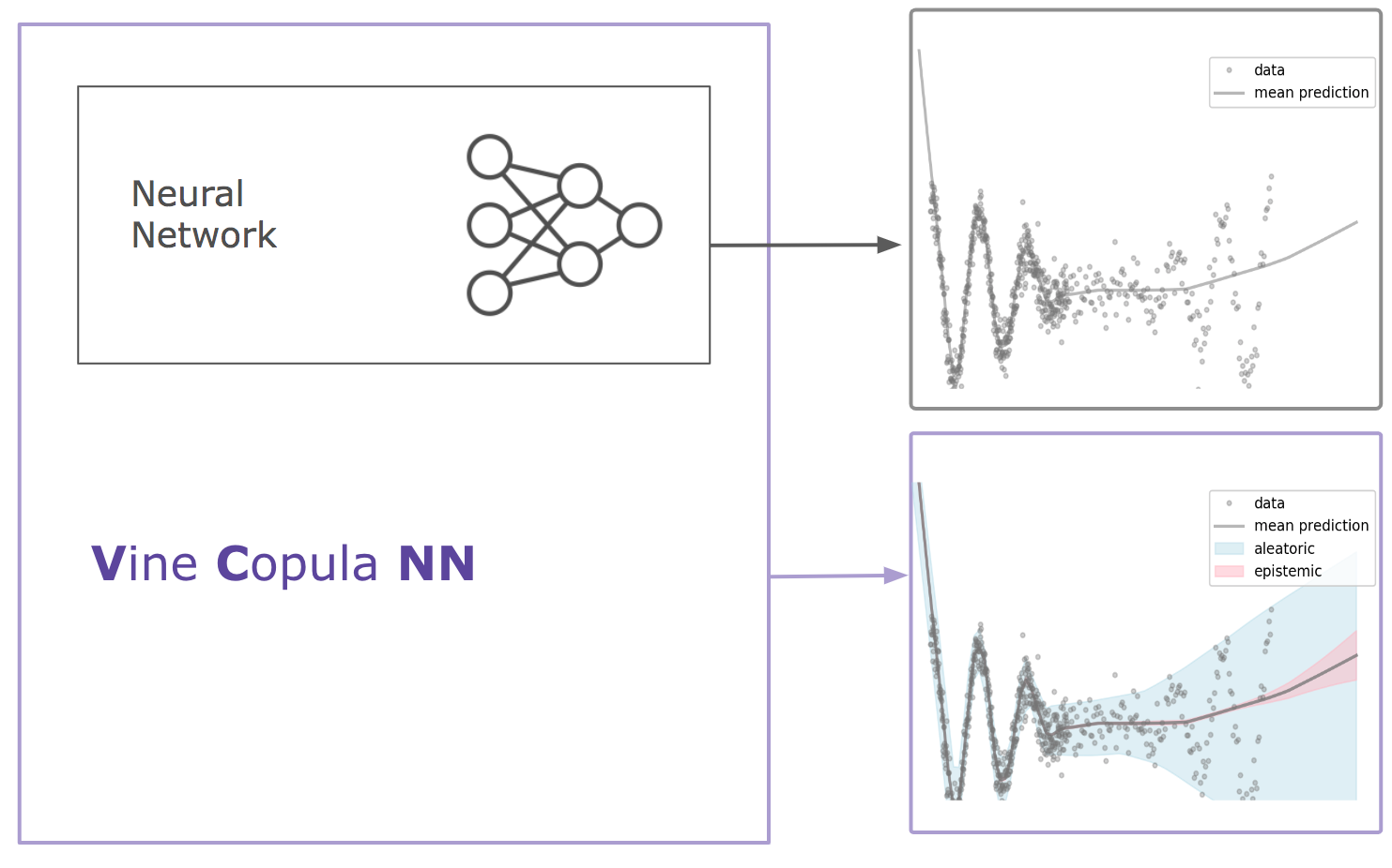
Figure 1: VCNN: We propose a plug-in vine-copula module that can complement any neural network with uncertainty estimates, any time after a model has been trained, without requiring any modifications to it. Additionally, our intervals capture both - aleatoric and epistemic uncertainty.

Typically, a NN does not quantify uncertainty, but merely provides point estimates as predictions. The predictive uncertainty, associated with the errors of a model, originates from two probabilistic sources:

• an epistemic one - the data provided in the training is not complete, i.e. certain input regions have not been covered in the training data, or the model lacks the capacity to approximate the true function (lack of knowledge, hence, reducible);

• an aleatoric one, resulting from the inherent noise in the data, hence, an irreducible quantity, but, can be accounted for.

To use NNs for applications in any domain, it is essential to provide uncertainty statements related to both of these sources. Nowadays, the most popular approaches for overall uncertainty estimation used by practitioners are MC-dropout [Gal and Ghahramani, 2016, Kendall and Gal, 2017], ensembles [Lakshminarayanan et al., 2017] and Bayesian NNs [Hernández-Lobato and Adams, 2015]. Each of these approaches comes at a price, whether in terms of accuracy or computation time, as summarised in Table 1.

This work is an attempt to alleviate those costs, reclaiming uncertainties for any deterministic model, retrospectively, by complementing it with a vine copula [Joe and Kurowicka, 2011]. We favor vine copulas for the flexible estimation (parametric and non-parametric) as well as the (theoretically justified) scalability.

We use Table 1 to position the unique properties of having vine copula uncertainty estimates. The vine copula provides an elegant way to extend any trained network retrospectively by quantifying both epistemic and aleatoric uncertainties, with performance on par or better than popular baselines. Given the undesired training costs of deeper and wider NNs, VCNN strikes as a viable solution. which is particularly attractive given the increasing training costs (both financial and environmental) of NNs.

It is also important to note that although there are many recent developments regarding the uncertainty of deep models, only a few consider the two sources (aleatoric and epistemic), and even fewer have a unifying framework for both of them. This is why, in sciences and industry which require both, Bayesian NNs prevail regardless of their heavy implementation. Motivated by this practical problem, our contributions are as follows:

• A new methodology for recovering uncertainties in deep models based on vine copulas (section 3),

• An implementation of plug-in uncertainty estimates (algorithm 1),

• Empirical evaluation on real-world datasets (section 4).

2 BACKGROUND

Problem setup We consider a supervised learning setup where $X\in\mathbb{R}^{p}$ is a random variable for the features, and $Y\in\mathbb{R}$ is the target variable. We assume a process $y=f(x,\epsilon)$ to be responsible for generating a dataset $\mathcal{D}=\{{x_{i},y_{i}\}}_{i=1}^{N}$ from which we observe realizations. We are interested in learning a prediction model for $f:\mathcal{X}\rightarrow\mathcal{Y}$. In particular, to approximate $f$, we chose a (deep) neural network, with its weights considered as model parameters $\Theta$. The DNN can learn a model that approximates the conditional mean well, i.e $\hat{f}_{\Theta}\in\operatorname*{arg\,min}_{f}\ell(\hat{f}_{\Theta}(x),y)$ by setting the loss $\ell$ to mean-squared error.

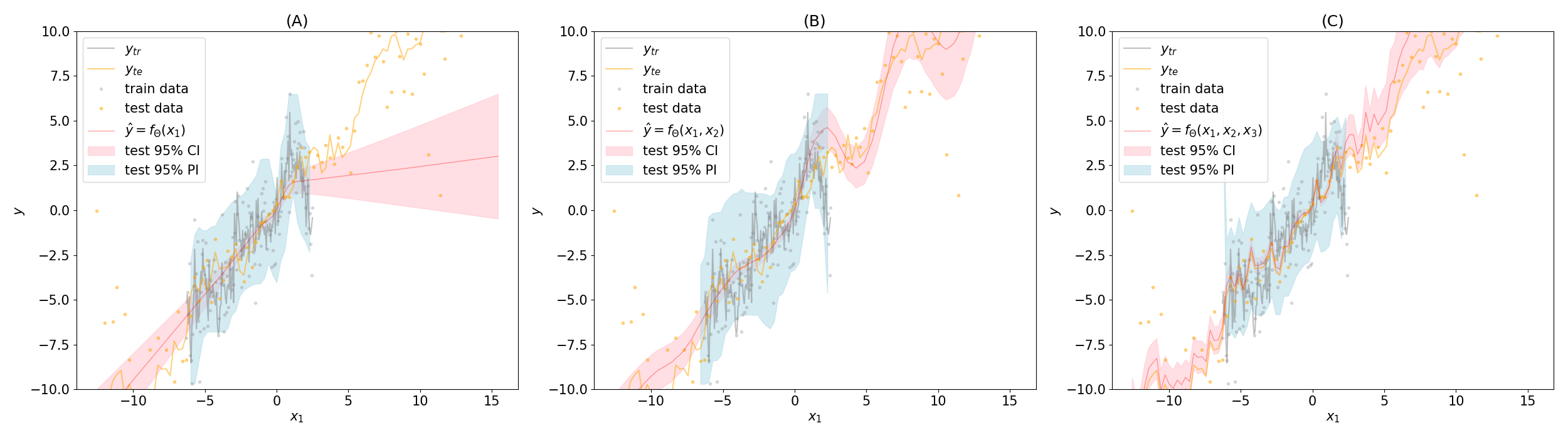
Figure 2: Confidence and Prediction intervals by VCNN in a toy regression problem. Data generated as: $Y_{train}=X_{1}+X_{2}+X_{3}+\epsilon$, with $X1=\mathcal{U}[-2\pi,2\pi]$, $X_{2}=sin(2X_{1})$, $X_{3}\sim sin(X_{1}^{2})$, with $\epsilon\sim\mathcal{N}(0,0.2)$. For the test data $Y_{train}=X_{1}+X_{2}+X_{3}+x_{1}\epsilon$, with $X1\sim\mathcal{U}[-4\pi,5\pi]$, $X_{2}=sin(X_{1})$, $X_{3}\sim sin(X_{1}^{2})$, with $\epsilon\sim\mathcal{N}(0,0.5)$. Train data consists of 280 samples, and the test of 100. The network was trained for 100 epochs for the three presented cases.

Within standard statistical models, one could relate the epistemic uncertainty to confidence intervals (CIs) which evaluate the $Pr(f(x)|\hat{f}(x))$, whereas the aleatoric, noise uncertainty is captured by prediction intervals (PIs) $Pr(y|\hat{f}(x))$. Both of these uncertainties contribute to the variability in the predictions which can be expressed through entropy or variance [Depeweg et al., 2018]. In this work, we will use the variance $\sigma^{2}$, as a quantity of interest unifying the two sources of uncertainty, and represent the overall predictive uncertainty per data point by its lower bound $\displaystyle L:=\min_{i\in N}({\sigma^{2}_{e^{i}}},{\sigma^{2}_{a^{i}}})$ and its upper bound $\displaystyle U:=\max_{i\in N}({\sigma^{2}_{e^{i}}},{\sigma^{2}_{a^{i}}})$, where $a$ stands for aleatoric (data related uncertainty) and $e$ for epistemic ( model uncertainly). Our goal is to propose a tool that recovers estimates for both the confidence and the prediction intervals of a DNN. This natural decomposition wrt variance will further allow for them to be combined and used in applications as deemed most suitable. We summarize our method VCNN in Figure 1.

We propose Figure 2 to exemplify the sources and respective uncertainty estimates in more detail. The observations are following a wiggly sequential data where the true generative process is a function $f(X_{1},X_{2},X_{3},\epsilon)$ which we try to predict with a DNN of 2 hidden layers with 50 neurons each. Moving from left to right, the plots in Figure 2 show the network predictions given: A) only observations from $X_{1}$ as input, i.e. $\hat{y}=\hat{f}_{\Theta}(x_{1})$, then $\hat{y}=\hat{f}_{\Theta}(x_{1},x_{2})$ in B, and $\hat{y}=\hat{f}_{\Theta}(x_{1},x_{2},x_{3})$ in C. By including relevant variables (more knowledge; more data), the fitted model improves in each consecutive plot, visible also through its CI and PI. This toy example shows the sensitivity of our estimates to both sources: As the DNN gets more information, the prediction of the model improves, its CIs improve as well (narrower in train region, wider outside), while the PIs capture the noisiness of the data (when variables are omitted, such as in A and B, this translates into more stochasticity, i.e as aleatoric noise). Moreover, from Figure 2, we also see why considering both sources is important: in the out-of-distribution region, the confidence intervals prevail, while in the nosier regions, the prediction intervals envelop the CI.

Next, we present how we envision using the natural properties of vine-copulas to account for the uncertainties of a deep model. We assume that a DNN, $\hat{f}_{\Theta}$, has already been trained until convergence for a specific task. Our goal is to supplement the output of the already-trained network, with trustworthy uncertainty estimates. For efficiency and simplicity of the method, we use the embeddings from the last hidden layer of the network - $\xi$, (where $\xi=h(x)\in\mathbb{R}^{d},d<<p$) as a proxy for the overall network parameters.

2.1 Copulas and Vines

According to Sklar’s theorem [Sklar, 1959], the joint density of any bivariate random vector $(X_{1},X_{2})$, can be expressed as

$$f(x_{1},x_{2})=f_{1}(x_{1})f_{2}(x_{2})c(F_{1}(x_{1}),F_{2}(x_{2}))$$ (1)

where $f_{i}$ are the marginal densities, $F_{i}$ the marginal distributions, and $c$ the copula density. That is, any bivariate density is uniquely described by the product of its marginal densities and a copula density, which is interpreted as the dependence structure. Figure 3 illustrates all of the components representing the joint density. As a benefit of such factorization, by taking the logarithm on both sides, one could straightforwardly estimate the joint density in two steps, first for the marginal distributions, and then for the copula. Copulas are widely used in finance and operation research, and, in the machine learning community have recently been integrated with deep models for generative and density estimation purposes [Tagasovska et al., 2019, Janke et al., 2021, Drouin et al., 2022, Ng et al., 2022]. Hence, copulas provide means to flexibly specify the marginal and joint distribution of variables. For further details, please refer to [Aas et al., 2009, Joe et al., 2010].

There exist many parametric representations through different copula families, however, to leverage even more flexibility, in this paper, we focus on kernel-based nonparametric copulas of [Geenens et al., 2017]. Equation 1 can be generalized and holds for any number of variables. To be able to fit densities of more than two variables, we make use of the pair copula constructions, namely vines; hierarchical models, constructed from cascades of bivariate copula blocks [Nagler et al., 2017]. According to [Joe, 1997, Bedford and Cooke, 2002], any $d$ dimensional copula density can be decomposed into a product of $\frac{d(d-1)}{2}$ bivariate (conditional) copula densities. Although such factorization may not be unique, it can be organized in a graphical model, as a sequence of $d-1$ nested trees, called vines. We denote a tree as $T_{m}=(V_{m},E_{m})$ with $V_{m}$ and $E_{m}$ the sets of nodes and edges of tree $m$ for $m=1,\dots,d-1$. Each edge $e$ is associated with a bivariate copula. An example of a vine copula decomposition is given Figure 4.

In practice, in order to construct a vine, one has to choose two components:

1. the structure, the set of trees $T_{m}=(V_{m},E_{m})$ for $m=1,\dots,d-1$

2. the pair-copulas, the models for $c_{j_{e},k_{e}|D_{e}}$ for $e\in E_{m}$ and $m=1,\dots,d-1$.

Corresponding algorithms exist for both of those steps and in the rest of the paper, we assume consistency of the vine copula estimators for which we use the implementation by [Nagler and Vatter, 2018a].

3 VINE-COPULA UNCERTAINTY ESTIMATES

3.1 Simulation-based Confidence Intervals

Besides being a flexible density estimation method, (vine) copulas additionally have generative properties [Dissmann et al., 2013]. That means that once a copula is fit on a data distribution, it can be used to produce random observations from it. Although mainly used for stress testing in the finance domain, this property of copulas has recently been recognized as a useful high dimensional generative model for images [Tagasovska et al., 2019]. Hence, this served as an inspiration to use vine copulas to bootstrap the network parameters, yielding confidence intervals for its predictions via simulations. Simulation-based approaches for confidence intervals have previously been used in the literature for smoothing splines [Ruppert et al., 2003].

Following a similar approach to [Ruppert et al., 2003], we consider the true function $f$ over $L$ locations in $x$, $\mathbf{l}=\{{l_{1},l_{2},\dots l_{L}\}}$, $f_{\mathbf{l}}$ denoting the vector of evaluations of $f$ at each of those locations, and the corresponding estimate of the true function by the trained DNN as $\hat{f}_{\Theta_{\mathbf{l}}}$. The difference between the true function and our unbiased estimator is given by:

$$\hat{f}_{\Theta_{\mathbf{l}}}-f_{\mathbf{l}}=H_{\mathbf{l}}\begin{bmatrix}\hat{\Theta}-\Theta\ \end{bmatrix}$$

where $H_{\mathbf{l}}$ is the evaluation of the DNN at the locations $\mathbf{l}$, and the expression in brackets represents the variation in the estimated network parameters. The distribution of the variation is unknown, and we aim to approximate it by simulation.: A $100(1-\alpha)\%$ simultaneous confidence interval is:

$$\hat{f_{l}}\pm q_{1-\alpha}\hat{\sigma}[(\hat{f}(l_{j})-f(l_{j})]_{j=1}^{L}$$ (2)

where $\sigma$ denotes a standard deviation and $q_{1-\alpha}$ is the $1-\alpha$ quantile of the random variable:

$$\sup_{x\in X}\begin{vmatrix}\frac{\hat{f}(x)-f(x)}{\hat{\sigma}(\hat{f}(x))-f(x)}\end{vmatrix}\approx\max_{1\leq j\leq L}\begin{vmatrix}\frac{H_{l}\begin{bmatrix}\hat{\Theta}-\Theta\\ \end{bmatrix}_{j}}{\hat{\sigma}\hat{f}(l_{j})-f(l_{j}))}\end{vmatrix}.$$ (3)

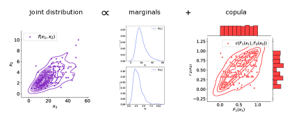
Figure 3: Expressing joint densities with copulas.

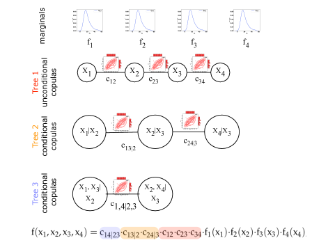
Figure 4: Multivariate joint density factorized with a vine copula.

The $\sup$ refers to the supremum or the least upper bound; which is the least value of $x$ from the set of all values which we observed, which is greater than all other values in the subset. Commonly, this is the maximum value of the subset, as indicated by the right-hand side of the equation. Hence we want the maximum (absolute) value of the ratio overall values in $\mathbf{l}$. The fractions in both sides of the equation correspond to the standardized deviation between the true function and the model estimate, and we consider the maximum absolute standardized deviation. While we do not have access to the distribution of the deviations, we only need its quantiles that we can approximate via simulations.

Herein, we exploit the generative nature of copulas whereby we “bootstrap” the trained DNN with the vine copula fitted over the embeddings $\xi=h(x)$ (the embeddings of a data point $x$ in the last hidden layer) and target $y$. For each simulation, we find the maximum deviation of the (re)-fitted functions from the true function over the grid of $\mathbf{l}$ values we are considering.

As the last step, we find the critical value to scale the standard errors $SE$ such that they yield the simulation interval; we calculate the critical value $r$ for a 95% simulation confidence interval using the empirical quantile of the ranked standard errors. Finally, we recover the upper and lower epistemic bounds obtained as:

$$\definecolor{tcbcol@origin}{rgb}{0,0,0}\definecolor{.}{rgb}{0,0,0}\definecolor{.}{rgb}{0,0,0}\leavevmode\hbox to175.16pt{\vbox to29.92pt{\text{[drawing]}}}. y_{Ue}/y_{Le}=\hat{f}_{\Theta}(x)\pm r*SE(H_{l}\begin{bmatrix}\hat{\Theta}-\Theta\ \end{bmatrix}) y_{Ue}/y_{Le}=\hat{f}_{\Theta}(x)\pm r*SE(H_{l}\begin{bmatrix}\hat{\Theta}-\Theta\ \end{bmatrix})$$ (4)

3.2 Conditional-quantile Prediction Intervals

In the case of predictive aleatoric uncertainty, we are interested in estimating the conditional distribution of the target variable given the inputs $F(Y|X)$, which is captured by conditional quantiles of interest [Tagasovska and Lopez-Paz, 2019]. Since we are aiming for a unified framework for uncertainties, we wish to also derive the necessary quantile predictions from vine-copula representations. To do so, we use the recent development by [Nagler and Vatter, 2018b] which shows that conditional expectations can be replaced by unconditional ones, and such property can be used to leverage copulas for solving regression problems. This approach allows for new estimators of various nature, such as mean, quantile, expectile, exponential family, and instrumental variable regression, all based on vine-copulas. Regression problems can be represented as solving equations:

$$\mathbb{E}\{g_{\phi}(Y)|X\}=0$$

where $\phi$ is a parameter of interest and the set $\mathcal{G}=\{g_{\phi}:\phi\in\Phi\}$ is a family of identifying functions. Conditional expectations can be replaced by the less challenging to estimate, unconditional ones as follows:

$$\mathbb{E}\{g_{\phi}(Y)|X\}=\mathbb{E}\{g_{\phi}(Y)w^{*}(Y)\}$$

with

$$w^{*}(y)=\frac{dF_{Y|X}(y|x)}{dF_{Y}(y)}=\frac{dF_{Y,X}(Y,X)}{dF_{X}(x)dF_{Y}(y)}.$$ (5)

Given the background on copulas, we see that the weights in Equation 5 can be expressed with:

$$w^{*}(y)=\frac{dC_{Y,X}(F_{Y}(y),F_{X}(x))}{dF_{C_{X}}(F_{X}(x))dF_{C_{Y}}(F_{Y}(y))}.$$

This expression can be further simplified by dropping $C_{X}$ as it does not depend on $y$ or $\phi$, and because copulas have uniform margins; we are left with $w^{*}(y)=dC_{Y,X}(F_{Y}(y),F_{X}(x))$. As exemplified in [Nagler and Vatter, 2018b], with different identifying functions $g_{\phi}$, we get estimators $\hat{\phi}=\hat{\phi}(Y_{1},X_{1},\dots,Y_{n},X_{n})$ to various conditional distributions as solutions to $\frac{1}{n}\sum_{i=1}^{N}g_{\phi}(Y_{i})w(Y_{i})=0$ . Here, we rely on solving estimating equations when the identifying function $g_{\phi}$ is suitable for quantile regression. We thus let:

$$\phi_{\tau}=F^{-1}_{Y|X}(\tau|X=x)$$

be the conditional $\tau-$quantile for $\tau\in(0,1)$, all levels considered jointly. Using this knowledge, and the embeddings $\xi$ as conditioning variables, we are now able to compute the upper and lower bound of a required $(1-\alpha)$ prediction interval, by obtaining:

(6)

solving this conditional expectation using vine copulas. In practice, we use the recent implementation from the eecop package [Nagler and Vatter, 2020].

With the expressions capturing both uncertainty estimates, we finally summarize our method VCNN, computing both epistemic and aleatoric uncertainties per data point in Algorithm 1.

Inputs: DNN $\hat{f}_{\Theta}$, train samples $\{{x_{i},y_{i}\}}_{i=1}^{N}$, test samples $\{{x_{j}^{\prime}\}}_{j=1}^{L}$;

Step 1. Obtain embeddings from the last dense layer, before the activations, $\xi=\{{h(x_{i})\}}_{i=1}^{N}\in\mathbb{R}^{d}$;

Step 2. Fit a vine copula with the embeddings and target variable, $V:=C(\xi_{1},\xi_{2},\dots\xi_{d},y)$. ;

Epistemic uncertainty ;

Step 3. For $S$ repetitions:

1. Sample random observations from the vine $V$, $\{{\xi^{*},y^{*}\}}$.

2. Re-train the last hidden and the output layer of $\hat{f}_{\Theta}$ with $\{{\xi^{*},y^{*}\}}$ .

3. Save the bootstraped $S$ headsof the network.

Step 4. Compute the confidence interval (CI) bounds: $y_{Le}(x^{\prime})$ and $y_{Ue}(x^{\prime})$ with Equation 4. ;

Aleatoric uncertainty ;

Step 5. Compute the prediction interval (PI) bounds: $y_{La}(x_{j}^{\prime})$ and $y_{Ua}(x_{j}^{\prime})$ by solving for the required quantiles $F^{-1}_{1-\frac{\alpha}{2}}(Y|\xi(x^{\prime}))$ and $F^{-1}_{\frac{\alpha}{2}}(Y|\xi(x^{\prime}))$ using vine $V$ with Equation 6.

Outputs $S$-heads, vine copula $V$, confidence and prediction intervals for $x^{\prime}$.

Algorithm 1 Vine-copula DNN uncertainty estimates.

4 EXPERIMENTS

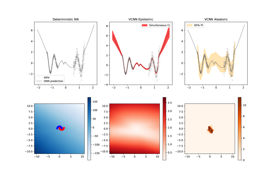
Figure 5: VCNN for toy regression and classification scenarios.

To empirically evaluate our method we propose three setups: synthetic toy examples for regression and classification, and, two real-world datasets: Datalakes - estimating the surface temperature of Lake Geneva based on sensor measurements, hydrological simulations and satellite imagery, and an AirBnB apartment price forecasting dataset. In all cases we wish to estimate the predictive uncertainty, hence, we account for both epistemic and aleatoric uncertainty sources. As baselines, we use Deep Ensembles [Lakshminarayanan et al., 2017], MC-dropout [Kendall and Gal, 2017] and Bayesian NN [Hernández-Lobato and Adams, 2015], all adjusted to capture the two types of uncertainties, simultaneously. Our code and demo for VCNN are available on https://github.com/tagas/vcnn.

Metrics

To compare baselines we use the number of points captured by the prediction intervals (PI), which should capture some desired proportion of the observations, $(1-\alpha)$.

$$Pr(\hat{y}_{L^{i}}\leq y_{i}\leq\hat{y}_{U^{i}})=(1-\alpha)$$

In all experiments except if stated otherwise, we target the common choice $\alpha=0.05$. To evaluate the quality of the PIs, similarly to [Pearce et al., 2018], we denote a vector, $\mathbf{k}$, of length $n$ which represents whether each data point has been captured by the estimated PIs, with NO $k_{i}\in[0,1]$ given by,

$$k_{i}=\begin{cases}1,&if\quad y_{L^{i}}\leq y_{i}\leq y_{U^{i}}\\ 0,&otherwise.\end{cases}$$

We denote the total number of points captured as $c=\sum_{i=1}^{n}k_{i}$. With this, we can now define the two main metrics we will use:

• The Prediction Interval Coverage Probability - $PICP:=\frac{c}{n},$ - which indicates how many of the observations are captured inside the estimated interval. A coverage closer to the desired proportion (set by $\alpha$) is preferred;

• The Mean Prediction Interval Width -

  $$MPIW:=\frac{1}{n}\sum_{i=1}^{n}\hat{y}_{U^{i}}-\hat{y}_{L^{i}},$$

  - which indicates how tight are the predicted intervals, where lower values are better.

Baselines

In general, the proposed baselines (Ensembles and MC Dropout) capture the epistemic and aleatoric uncertainty jointly. Regarding the aleatoric uncertainty, these baselines consider DNN with outputs being the conditional parameters of a normal distribution, $\mathcal{N}(\mu_{\Theta},\sigma_{\Theta})$. On the other hand, each baseline models the epistemic uncertainty in a different way (due to random initialisation).

For the sake of a fair comparison, we let both baseline functions, $\mathcal{N}(\mu_{\Theta},\sigma_{\Theta})$ have as input the embedding of the last dense layer, $\xi$, similar to Algorithm 1.

Heteroscedastic Deep Ensemble

(Ensemble+N) consists of a set of $S$ functions pairs, $\{(\mu_{\Theta,i},\sigma_{\Theta,i})\}_{i=1}^{S}$, such that each pair is trained (1) on a different split from the training data set and (2) with different parameters initialization, in order to maximize the diversity between the individual pairs (which also includes the bootstrap[Ganaie et al., 2021]).

Heteroscedastic Monte-Carlo Dropout

(MCDrop+N) outputs the pair, $\{(\mu_{\Theta,i},\sigma_{\Theta,i})\}_{i=1}^{S}$, where each $i$ corresponds to a different, randomly selected connection, implemented as dropout layers. Differently than the Ensemble+N, here we considered the whole training set as proposed in [Gal and Ghahramani, 2016].

Bayesian Neural Network

(Bayesian NN+N) outputs the pair, $\{(\mu_{\Theta,i},\sigma_{\Theta,i})\}_{i=1}^{S}$, where each $i$ corresponds to a different, randomly selected sample from the random variables associated to all neuron weights. In particular, this random variable has a prior and posterior normal distribution optimized via variational inference [Graves, 2011].

4.1 Toy example

In Figure 5 we include the evaluation of VCNN on toy examples. The first row is a one-dimensional input bi-modal regression task, while the second row is a classification task for a two-dimensional input, namely the moons dataset. We show the results from a deterministic DNN (predictions and class probabilities respectively) in the first column, the epistemic uncertainty estimate in the second, and the aleatoric uncertainty estimate in the third obtained with vine copulas. For the classification task, since the input is two-dimensional, we present the uncertainty scores through a color range, depicting the distance between the upper and lower bounds of the corresponding CI or PI. We consider these classification results encouraging, since both the epistemic uncertainty grows further away from the train data, and the aleatoric uncertainty is high only in the region where there is an overlap between the two classes, as expected.

4.2 Datalakes

Datalakes tackles certain data-driven problems such as estimating lake surface temperature given a range of sensory, satellite imagery, and simulation-based datasets. One such dataset is of Lake Geneva where a sparse hourly dataset is collected between years 2018 to 2020. Given the temporal nature of the observations, the model that provided the best prediction was a bidirectional (Bi)[Schuster and Paliwal, 1997] long short-term memory (LSTM)[Hochreiter and Schmidhuber, 1997] network. Originally, this method uses MC-dropout in addition to a negative log-likelihood loss as in [Kendall and Gal, 2017]. We replace those uncertainties with the vine based ones and we present our results in Table 2. Comparisons with ensemble methods were omitted due to both computational restrictions and the MC-dropouts method being a comparable proxy. From Table 2 we see that the VCNN achieves on-par estimates for PICP with (significantly) narrower interval widths as suggested by the MPIW. The measuring unit is Celsius degrees.

Table 2: PICP and MPIW values for VCNN and baselines for the real-world datalakes dataset. Note that the very long training of the biLSTM network did not allow for multiple executions for obtaining std variations or results from ensembles.

BiLSTM	Train		Test
	PICP	MPIW	PICP	MPIW
VCNN	.97	5.71	.85	5.84
MC-Dropout+N	.94	6.97	.86	6.88

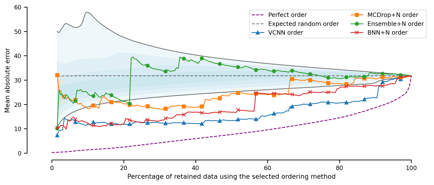
Figure 6: Error-retention curves - considering the mean cumulative error for the most confident points and sorting using the uncertainty scores -, which are produced by the baselines and the VCNN (see [Brando et al., 2018, Brando, 2022])

.

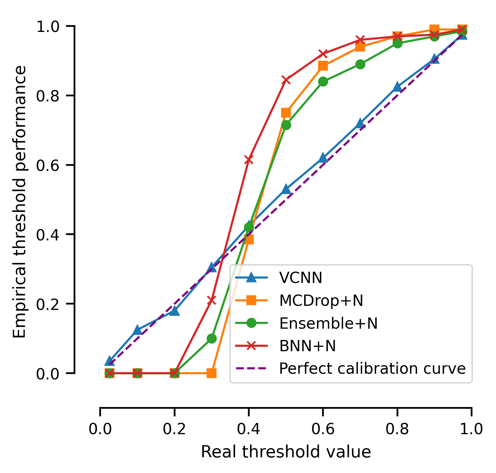
Figure 7: Calibration curves of the baselines and the VCNN using their forecasted quantiles (see [Brando et al., 2022]).

4.3 Room price forecasting

Based on publicly available data from the Inside Airbnb platform [Cox, 2019], for Barcelona, we followed a regression problem proposed in [Brando et al., 2019]. The aim is to predict the price per night for $36,367$ flats using data from April 2018 to March 2019. The architecture used is a DenseNet, detailed in the Supplementary Material section. From Table 3 we notice that the plug-in estimates of VCNN outperform the Bayesian NNs, ensembles and MC-dropout - VCNN intervals are properly calibrated (targeting the 95%) and they are tighter by at least a half. The measurement unit here is euros.

Table 3: PICP and MPIW (mean and std. dev) for VCNN and baselines for the real-world Airbnb dataset.

DenseNet	Train		Test
	PICP	MPIW	PICP	MPIW
Bayesian NN+N	$.99\pm.00$	$698.45\pm 93.$	$.99\pm.00$	$645.55\pm 73.$
MC-Dropout+N	$.99\pm.00$	$468.03\pm 49.$	$.99\pm.00$	$514.15\pm 72.$
Ensemble+N	$.99\pm.00$	$433.25\pm 27.$	$.98\pm.00$	$468.95\pm 31.$
VCNN	$\bm{.97\pm.01}$	$\bm{226.8\pm 4.4}$	$\bm{.95\pm.00}$	$\bm{191.33\pm 3.0}$

4.4 Evaluating the quality of uncertainty intervals

Additionally, we can evaluate the quality of the reported uncertainty by leveraging this information as a confidence score. To accomplish this, we analyze an error-retention curve [Brando, 2022]. This curve involves computing the normalized cumulative absolute errors in ascending order of their corresponding uncertainty scores, such that the individual error with the highest uncertainty score with respect to the selected ordering method appears at the end of the list. Moreover, we observe in Figure 6, that the VCNN exhibits an error-retention curve that consistently approximates the perfect curve, to a greater extent than other baselines. This plot reads as follows: with a perfect confidence score, we can retain 80% of the data points and expect an MAE of 14 euros. For the same amount of data, with VCNN we expect MAE of 18 euros, and with all other baselines MAE $>25$.

Finally, since for the AirBnB dataset all baselines can be trained in a reasonable time (including ensembles), we show a calibration plot in Figure 7. Calibration lines are crucial to ensure proper behavior of the predicted quantiles, by plotting the model’s predictions against the empirical quantile values. The results in Figure 7 show that VCNN forecasts are closer to the perfect calibration line while Ensembles, MC dropout, and Bayesian NNs underestimate quantiles lower than the median and are overconfident for quantiles above 0.5.

4.5 Practical considerations for the vine copulas

Complexity The complexity for fitting the vine copulas as currently implemented is approximate $O(n\times dim\times vinedepth)$ for estimation/sampling algorithms, both involving a double loop over-dimension/truncation level with an internal step scaling linearly with the sample size. Due to this linear scaling in the number of samples and dimensions, we found it useful to randomly subsample the train data and use truncated vines. The runtimes of VCNN could greatly benefit of implementation optimizations, however, this is outside of the scope of the current work.

Hyperparameters

Although the vine structure and the copula family could be considered as hyperparameters, empirically we observed that the best results are obtained when we use nonparametric family with a low multiplier for the kernel width, i.e. 0.1, for both the confidence and prediction intervals. For computational purposes, we also chose to truncate the vine, that is to fit only the first 2 - 5 trees in the vine and consider all the subsequent ones as independent copulas. These factors can indeed appear as more important for other datasets and we are conducting multiple ablation studies to explore this further.

5 CONCLUSION

In this work, we present new, plug-in uncertainty estimates for neural networks using vine copulas which can be applied to any network retrospectively. Importantly, our estimates do not impact the performance of the original model in any way, while they manage to enhance it with faithful predictive confidence measures. This is particularly attractive given the increasing training costs (financial and environmental) with deeper and wider NNs.

We hope our method can help in increasing the trustworthiness of deep models, specifically for real-world scenarios which render critical decision-making. There are multiple directions for extensions: out-of-distribution detection methods in classification tasks underlying different architectures (image, graph), and, we expect VCNN to improve results in other tasks relying on uncertainties, such as segmentation or active learning.

6 SUPPLEMENTARY MATERIAL

6.1 Example of a Vine Copula

A sequence is a vine if it satisfies the set of conditions which guarantee that the decomposition represents a valid joint density: i) $T_{1}$ is a tree with nodes $V_{1}=\{1,\dots,d\}$ and edges $E_{1}$ ii) For $m\geq 2$, $T_{m}$ is a tree with nodes $V_{m}=E_{m-1}$ and edges $E_{m}$ iii) Whenever two nodes in $T_{m}+1$ are joined by an edge, the corresponding edges in $T_{m}$ must share a common node. The corresponding tree sequence is the structure of the vine. Each edge $e$ is associated to a bivariate copula $c_{j_{e},k_{e}|D_{e}}$, with the set $D_{e}\in\left\{1,\cdots,d\right\}$ and the indices $j_{e},k_{e}\in\left\{1,\cdots,d\right\}$ forming respectively its conditioning set and the conditioned set. Finally, the joint copula density can be written as the product of all pair-copula densities $c(u_{1},\cdots,u_{d})=\prod_{m=1}^{d-1}\prod_{e\in E_{m}}c_{j_{e},k_{e}|D_{e}}(u_{j_{e}|D_{e}},u_{k_{e}|D_{e}})$ where $u_{j_{e}|D_{e}}=\mathbb{P}\left[U_{j_{e}}\leq u_{j_{e}}\mid\bm{U}_{D_{e}}=\bm{u}_{D_{e}}\right]$ and similarly for $u_{j_{e}|D_{e}}$, with $\bm{U}_{D_{e}}=\bm{u}_{D_{e}}$ understood as component-wise equality for all components of $(U_{1},\dots,U_{d})$ and $(u_{1},\dots,u_{d})$ included in the conditioning set $D_{e}$.

For self-contained manuscript, we borrow from [Tagasovska et al., 2019], a full example of an R-vine for a 5-dimensional density.

Example:

The density of a PCC corresponding to the tree sequence in Figure 8 is

$$c ={\color[rgb]{1,0,0}c_{1,2}\,c_{1,3}\,c_{3,4}\,c_{3,5}}\,{\color[rgb]{0,0,1}c_{2,3|1}\,c_{1,4|3}\,c_{1,5|3}}{\color[rgb]{0,1,0}c_{2,4|1,3}\,c_{4,5|1,3}}\,{\color[rgb]{1,0,1}c_{2,5|1,3,4}},$$ (7)

where the colors correspond to the edges $E_{1}$, $E_{2}$, $E_{3}$, $E_{4}$.

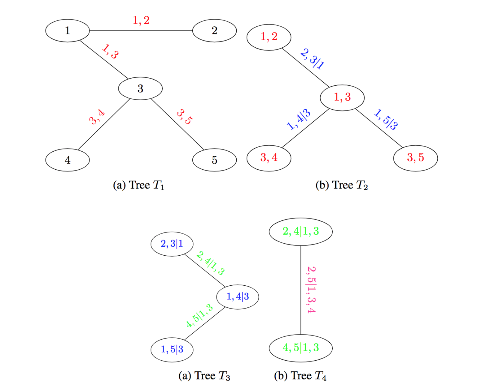
Figure 8: A vine tree sequence: the numbers represent the variables, $x,y$ the bivariate distribution of $x$ and $y$, and $x,y|z$ the bivariate distribution of $x$ and $y$ conditional on $z$. Each edge corresponds to a bivariate pair-copula in the PCC.

6.2 Details of the toy experiment in Figure 2

The toy example in Figure 2 is generated as: $Y_{train}=X_{1}+X_{2}+X_{3}+\epsilon$, with $X1=\mathcal{U}[-2\pi,2\pi]$, $X_{2}=sin(2X_{1})$, $X_{3}\sim sin(X_{1}^{2})$, with $\epsilon\sim\mathcal{N}(0,0.2)$. For the test data $Y_{train}=X_{1}+X_{2}+X_{3}+x_{1}\epsilon$, with $X1\sim\mathcal{U}[-4\pi,5\pi]$, $X_{2}=sin(X_{1})$, $X_{3}\sim sin(X_{1}^{2})$, with $\epsilon\sim\mathcal{N}(0,0.5)$. Furthermore, the train data consists of 280 samples, and the test data of 100. The network was trained for 100 epochs for the three presented cases, using Adam optimizer with default PyTorch parameters. We use $S$$=$$30$ to get the confidence intervals and $\tau_{low}=0.025$ and $\tau_{high}=0.975$ for the prediciton intervals.

6.3 Details BiLSTM implementation - Datalakes

Pre-RNN fully connected layers: 1 layer $\times$ 32 units, LeakyReLU ($\alpha=0.2$)
RNN layers: 3 LSTM layers $\times$ 32 units each and bidirectional ($\times$ 2 )
Dimensionality of last hidden layer: 64
Train and test data dimensions: 214,689 and 186,129 samples of 18 dimensions
Dropout level: 0.3
Rough estimate of train time: 6 days
VC fit time: 2634.29 sec;
VC inference time per data point: 2.1 sec
number of VC bootstraps: 15
Framework: Tensorflow 2.4.1

Due to the longer training times of the BiLSTM model and limited time and resources, we were not able to obtain standard variations of the results. Same reasoning goes for not recommending and including ensembles.

6.4 Details DenseNet implementation - AirBnB

The architecture used for the main DenseNet is the same that the proposed in [Brando et al., 2019]. Additionally, the different models proposed in this article satisfies the following parameters and results:

Number of layers: $6$ dense layers
Number of neurons per layer: $120,120,60,60,10$ and $1$
Training time: $30.4$ secs
Activation types: ReLU activation for hidden layers
Dimensionality of last hidden layer used by the VC: 10
Training , validation and test data dimensions: $29078$, $3634$ and $3633$ respectively.

VC estimates train time: $1861.09\pm 115.91$ secs.
Time of the VC predicting each point: $1.53\pm 3\cdot 10^{-3}$ secs
Number of VC bootstraps: $10$
Framework: Tensorflow 2.3

References

- [Aas et al., 2009] Aas, K., Czado, C., Frigessi, A., and Bakken, H. (2009). Pair-copula constructions of multiple dependence. Insurance: Mathematics and economics, 44(2):182–198.
- [Bedford and Cooke, 2002] Bedford, T. and Cooke, R. M. (2002). Vines – A New Graphical Model for Dependent Random Variables. The Annals of Statistics, 30(4):1031–1068.
- [Brando, 2022] Brando, A. (2022). Aleatoric Uncertainty Modelling in Regression Problems using Deep Learning. Barcelona university press.
- [Brando et al., 2022] Brando, A., Gimeno, J., Rodriguez-Serrano, J., Vitrià, J., et al. (2022). Deep non-crossing quantiles through the partial derivative. In International Conference on Artificial Intelligence and Statistics, pages 7902–7914. PMLR.
- [Brando et al., 2018] Brando, A., Rodríguez-Serrano, J. A., Ciprian, M., Maestre, R., and Vitrià, J. (2018). Uncertainty modelling in deep networks: Forecasting short and noisy series. In Joint European Conference on Machine Learning and Knowledge Discovery in Databases, pages 325–340. Springer.
- [Brando et al., 2019] Brando, A., Rodríguez-Serrano, J. A., Vitria, J., and Rubio, A. (2019). Modelling heterogeneous distributions with an uncountable mixture of asymmetric laplacians. NeurIPS.
- [Cox, 2019] Cox, M. (2019). Inside airbnb: adding data to the debate. Inside Airbnb [Internet].[cited 16 May 2019]. Available: http://insideairbnb.com.
- [Depeweg et al., 2018] Depeweg, S., Hernandez-Lobato, J.-M., Doshi-Velez, F., and Udluft, S. (2018). Decomposition of uncertainty in Bayesian deep learning for efficient and risk-sensitive learning. In ICML.
- [Der Kiureghian and Ditlevsen, 2009] Der Kiureghian, A. and Ditlevsen, O. (2009). Aleatory or epistemic? does it matter? Structural Safety.
- [Dissmann et al., 2013] Dissmann, J., Brechmann, E. C., Czado, C., Kurowicka, D., Dißmann, J., Brechmann, E. C., Czado, C., and Kurowicka, D. (2013). Selecting and estimating regular vine copulae and application to financial returns. Computational Statistics & Data Analysis, 59:52–69.
- [Drouin et al., 2022] Drouin, A., Marcotte, É., and Chapados, N. (2022). Tactis: Transformer-attentional copulas for time series. In International Conference on Machine Learning, pages 5447–5493. PMLR.
- [Gal, 2016] Gal, Y. (2016). Uncertainty in Deep Learning. PhD thesis, University of Cambridge.
- [Gal and Ghahramani, 2016] Gal, Y. and Ghahramani, Z. (2016). Dropout as a bayesian approximation: Representing model uncertainty in deep learning. In ICML.
- [Ganaie et al., 2021] Ganaie, M. A., Hu, M., et al. (2021). Ensemble deep learning: A review. arXiv preprint arXiv:2104.02395.
- [Geenens et al., 2017] Geenens, G., Charpentier, A., and Paindaveine, D. (2017). Probit transformation for nonparametric kernel estimation of the copula density. Bernoulli, 23(3):1848–1873.
- [Graves, 2011] Graves, A. (2011). Practical variational inference for neural networks. Advances in neural information processing systems, 24.
- [Guo et al., 2017] Guo, C., Pleiss, G., Sun, Y., and Weinberger, K. Q. (2017). On calibration of modern neural networks. ICML.
- [Havasi et al., 2020] Havasi, M., Jenatton, R., Fort, S., Liu, J. Z., Snoek, J., Lakshminarayanan, B., Dai, A. M., and Tran, D. (2020). Training independent subnetworks for robust prediction. arXiv preprint arXiv:2010.06610.
- [Hernández-Lobato and Adams, 2015] Hernández-Lobato, J. M. and Adams, R. (2015). Probabilistic backpropagation for scalable learning of bayesian neural networks. In ICML.
- [Hochreiter and Schmidhuber, 1997] Hochreiter, S. and Schmidhuber, J. (1997). Long short-term memory. Neural computation, 9 8:1735–80.
- [Hornik, 1991] Hornik, K. (1991). Approximation capabilities of multilayer feedforward networks. Neural Networks, 4(2):251–257.
- [Janke et al., 2021] Janke, T., Ghanmi, M., and Steinke, F. (2021). Implicit generative copulas. Advances in Neural Information Processing Systems, 34:26028–26039.
- [Joe, 1997] Joe, H. (1997). Multivariate Models and Dependence Concepts. Chapman & Hall/CRC.
- [Joe and Kurowicka, 2011] Joe, H. and Kurowicka, D. (2011). Dependence modeling: vine copula handbook. World Scientific.
- [Joe et al., 2010] Joe, H., Li, H., and Nikoloulopoulos, A. K. (2010). Tail dependence functions and vine copulas. Journal of Multivariate Analysis, 101(1):252–270.
- [Kendall and Gal, 2017] Kendall, A. and Gal, Y. (2017). What uncertainties do we need in bayesian deep learning for computer vision? In NeurIPS.
- [Lakshminarayanan et al., 2017] Lakshminarayanan, B., Pritzel, A., and Blundell, C. (2017). Simple and scalable predictive uncertainty estimation using deep ensembles. In NeurIPS.
- [Nagler et al., 2019] Nagler, T., Bumann, C., and Czado, C. (2019). Model selection in sparse high-dimensional vine copula models with an application to portfolio risk. Journal of Multivariate Analysis, 172:180–192.
- [Nagler et al., 2017] Nagler, T., Schellhase, C., and Czado, C. (2017). Nonparametric estimation of simplified vine copula models: comparison of methods. Dependence Modeling, 5(1):99–120.
- [Nagler and Vatter, 2018a] Nagler, T. and Vatter, T. (2018a). kde1d: Univariate Kernel Density Estimation. R package version 0.2.1.
- [Nagler and Vatter, 2018b] Nagler, T. and Vatter, T. (2018b). Solving estimating equations with copulas. arXiv preprint arXiv:1801.10576.
- [Nagler and Vatter, 2020] Nagler, T. and Vatter, T. (2020). eecop: an R Package to Solve Estimating Equations with Copulas. https://github.com/tnagler/eecop R package version 0.0.1.
- [Ng et al., 2022] Ng, Y., Hasan, A., and Tarokh, V. (2022). Inference and sampling for archimax copulas.
- [Pearce et al., 2018] Pearce, T., Zaki, M., Brintrup, A., and Neely, A. (2018). High-Quality Prediction Intervals for Deep Learning: A Distribution-Free, Ensembled Approach. In ICML.
- [Ruppert et al., 2003] Ruppert, D., Wand, M. P., and Carroll, R. J. (2003). Semiparametric regression. Number 12. Cambridge university press.
- [Schuster and Paliwal, 1997] Schuster, M. and Paliwal, K. K. (1997). Bidirectional recurrent neural networks. IEEE transactions on Signal Processing, 45(11):2673–2681.
- [Sklar, 1959] Sklar, A. (1959). Fonctions de Répartition à n Dimensions et Leurs Marges. Publications de L’Institut de Statistique de L’Université de Paris, 8:229–231.
- [Tagasovska et al., 2019] Tagasovska, N., Ackerer, D., and Vatter, T. (2019). Copulas as high-dimensional generative models: Vine copula autoencoders. NeurIPS 2019.
- [Tagasovska and Lopez-Paz, 2019] Tagasovska, N. and Lopez-Paz, D. (2019). Single-model uncertainties for deep learning. NeurIPS.